Efficient parameterised compilation for hybrid quantum programming
Abstract
Near term quantum devices have the potential to outperform classical computing through the use of hybrid classical-quantum algorithms such as Variational Quantum Eigensolvers. These iterative algorithms use a classical optimiser to update a parameterised quantum circuit. Each iteration, the circuit is executed on a physical quantum processor or quantum computing simulator, and the average measurement result is passed back to the classical optimiser. When many iterations are required, the whole quantum program is also recompiled many times. We have implemented explicit parameters that prevent recompilation of the whole program in quantum programming framework OpenQL, called OpenQL, to improve the compilation and therefore total run-time of hybrid algorithms. We compare the time required for compilation and simulation of the MAXCUT algorithm in OpenQL to the same algorithm in both PyQuil and Qiskit. With the new parameters, compilation time in OpenQL is reduced considerably for the MAXCUT benchmark. When using OpenQL, compilation of hybrid algorithms is up to two times faster than when using PyQuil or Qiskit.
1 Introduction
Even though Google announced quantum supremacy in 2019 [1], universal, fault-tolerant quantum computers are still a thing of the future. In the meantime, Noisy Intermediate-Scale Quantum (NISQ) devices like the Google Sycamore QPU have the potential to outperform classical computers in specific cases [3].
The NISQ era means that anybody writing quantum algorithms has to contend with a limited number of qubits and a trade-off between circuit depth and error-rates. The demonstration from Google on a 53-qubit chip had a fidelity of only 0.2%, for example [1].
Quantum algorithm development in the NISQ era is largely done with simulations of quantum devices, which are more readily available and still faster than real quantum devices for all cases where quantum supremacy has not been achieved. And many algorithms require more (interconnected) qubits than the current state-of-the-art has to offer. Besides, simulators offer other advantages, such as access to the full state of all qubits, error-free execution, setting of specific error rates and repeatability of "random" results [13].
One such area of quantum algorithm development is hybrid quantum-classical algorithms. These are expected to be the first algorithm candidates that will result in a practical application for quantum computation [6]. Current quantum computers have too few, too error-prone qubits to be sufficient to implement purely-quantum algorithms such as Shor’s factorisation algorithm [21] or Grover’s search algorithm [9]. But with hybrid algorithms, some of the processing is done on a classical computer, so quantum circuits with less qubits and lower depth are required for the quantum device and more fine-grained error correction can be applied [6].
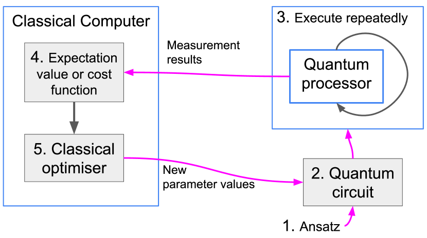
VQE, and other variational hybrid algorithms, require many iterations of the same quantum circuit. For each iteration, a set of parameters is updated according to some classical (optimisation) algorithm [6]. An example of the program flow for such algorithms is shown in Fig. 1.
Since compilers for quantum programming languages require a lot of processing to produce an executable quantum circuit, doing a full compilation each iteration consumes significant amounts of time. For iterative hybrid algorithms, however, most of the circuit stays the same between iterations, which means that error-correction mechanisms, optimisations, decompositions, mapping, etc. are not affected. For VQE specifically, only some angles for rotation gates are changed, which means that most compilation steps are not affected for parameterised gates.
With the increasing number of qubits quantum computers can support, and with increasing qubit quality, the depth and complexity of executable quantum circuits will increase. This in turn means that the amount of time spent during this recompilation step will continue to increase, making it necessary to optimise it as much as possible. At the same time, efficient classical compilation and simulation of quantum algorithms are essential tools in the NISQ era and beyond. For as long as quantum supremacy has not yet been reached, classical computers will continue to do part of the work.
In this paper we introduce OpenQL Parameterized Compilation (OpenQL) which reduces compilation time of hybrid quantum algorithms. The contributions of this paper are as follows:
-
•
A more efficient compilation process for parameterised hybrid quantum programming
-
•
Implementation of our method in the OpenQL quantum programming framework
-
•
Implementation of the MAXCUT quantum programming benchmark in OpenQL
This paper is structured as follows. A background on VQE and utilisation of parameters in programming languages is given in Section 2. Then the design and implementation of parameters in OpenQL are presented in Sections 3 and 4, respectively. The compilation process and improvements thereof can be found in Section 5. After that, the methods and results are discussed in Sections 6 and 7. The conclusion can be found in Section 8.
2 Background
To demonstrate the effect that a more efficient compilation of parameters can have, the VQE algorithm will be used. We will compare our implementation, OpenQL, against Qiskit (0.37.0) and PyQuil (3.1.0), so some background on these will be given as well.
2.1 Variational Quantum Eigensolvers
VQE is a class of hybrid quantum algorithms, i.e. it uses both classical and quantum resources, to find solutions to eigenvalue and optimisation problems. With VQE, quantum devices with as few as 40-50 qubits might outperform purely classical approaches [18]. VQE can run on any gate-model quantum device, is able to leverage the strengths of a specific architecture and to variationally suppress some errors [15]. To do this, it uses a parameterised quantum circuit, where the parameters are updated variationally according to a classical optimisation algorithm.
The execution flow of VQE is shown in Fig. 1. VQE can be used to determine the ground state and the ground state energy of a Hamiltonian . A Hamiltonian is a matrix describing the total energy of a (quantum) system. VQE has the following steps [15]:
-
1.
Pick a parameterised quantum state that is as close as possible to the solution, in this case the ground state of the Hamiltonian. This is . By adjusting the values of the parameter(s) , the state can become (closer to) the true problem solution. This parameterised state is the ansatz.
-
2.
Use the ansatz and the initial parameter values to generate a parameterised executable quantum circuit that will result in the state specified by the ansatz: .
-
3.
Repeatedly execute the circuit and measure the resulting state . This can be done by either:
-
(a)
Executing the circuit on a single quantum processor repeatedly and storing the results on a classical computer, or
-
(b)
Executing the circuit on many quantum processors simultaneously and collecting all measurement results on a classical computer.
-
(a)
-
4.
Use the results from the measurements to calculate the expectation (average) value of the quantum state, or use them to calculate the energy of the state through a cost function.
-
5.
Use a classical optimiser to determine new parameter values for the quantum circuit that will decrease the expectation value or the cost function result.
-
6.
Repeat step 2-5 until the difference between the results of subsequent iterations is smaller than the desired accuracy of the result. The final parameters determine the ground state of the Hamiltonian.
There are many options for the choice of ansatz, as well as the choice of classical optimiser. The ansatz can be tailored to many aspects of the algorithm and system used, such as the specific hardware implementation [15], specific problems, accuracy or circuit depth [8]. Different classical optimisers converge at different rates and respond differently depending on the amount of noise present in the quantum system [17].
The number of iterations before algorithm convergence depends on many different details. To give an indication, the qubit efficient implementation of VQE in [14] reaches the ground state in 500 iterations, with 17-qubit circuits that contain 180 to 900 variational parameters. The various VQEs from [10] are 6-qubit circuits with 30 parameters each done for 250 iterations, with measurements per iteration to estimate the expectation value.
However, for the purposes of verifying and measuring OpenQL, the specific details are not important. The choice was made to use the Nelder-Mead classical optimiser, because it is widely used and available in scipy.
2.2 Programming of parameterised circuits
In this paper, we compare OpenQL against Qiskit and PyQuil, the quantum programming languages from IBM and Rigetti, respectively. Both allow programming of parameterised circuits, are widely used and can be used as a library from a Python program. This makes them a good comparison to OpenQL, which also has these features.
The aim of OpenQL is to be easy to use for new quantum programmers as well as for people already familiar with these other languages. We will therefore give an overview of how parameters can be used in these other languages and aim to make our syntax similar so that adopting the new feature in OpenQL will be simple.
2.2.1 Qiskit
Qiskit is the quantum framework of IBM. It is suited for working with noisy qubits, which can be simulated using their simulator, Qiskit Aer. This allows classical simulation of circuits compiled using the Qiskit compiler, Qiskit Terra. Besides simulation, circuits compiled using Qiskit Terra can also be executed on real quantum devices using IBM Q [19].
In the following code listing, we show how parameterised circuits can be used in Qiskit:
Defining parameters in Qiskit can be done individually, as shown above on line 2, or as a vector with a specified length, as on line 3. Both can be used as gate arguments, as on lines 4 and 5 of the example. Binding parameters to values can be done using the command assign_parameters (line 6) to generate a single circuit, or by bind_parameters to generate a list of circuits with a circuit for each value of the parameter. This is shown on line 8. This code generates a list of 128 circuits, one for each of the values of theta as defined on line 7. The circuit can be output as OpenQASM to a file, as shown on line 8.
The circuits can be run on a real quantum system by compiling them individually for a specific backend. An example is shown here of how to run the circuits in the example above:
On line 1, one of the circuits is transpiled to be executable on the simulatorbackend. A list of circuits can also be compiled all at once, as on line 2. In both cases, the resulting compiled_circuit can be executed on any supported backend with the execute command, as shown in line 3. Any measurement results can be retrieved by calling result().get_counts() as on line 4. This gives the measurement results as counts of how often each possible bit combination was measured, for example: {’0’: 4, ’1’: 6}.
Compilation, execution and binding of parameter values can also be combined into a single execute command, as shown below:
Using a single command to bind parameters and simulate the circuit makes it impossible to determine the individual execution time of the components from the host Python program. So to get those results the separate commands are used. The compilation is considered complete after the assemble command.
2.2.2 PyQuil
PyQuil is the quantum programming language from Rigetti. It is compiled using the Quil compiler into Quil, also the name of their Quantum Instruction Language [23]. PyQuil can be used to write hybrid algorithms with parameters [11], which makes it a suitable comparison to OpenQL.
A PyQuil program with the same overall functionality as the one in Qiskit is shown below. The example program will be used to explain how parameters can be defined and used in PyQuil [22]:
A quantum program is defined on line 1. Two types of parameter are declared on lines 2 and 3; ro will be used to store the measurement results, and the parameter theta is used as argument for the RY gate on line 4.
The parameterised quantum program program from this example can be run for different values of theta, as shown in the following code listing [5]:
In line 1, the array parametric_measurements is defined for storing the measurement results. The program from the previous example is compiled for a specific execution platform, simulatorin this case. A for-loop is used to iterate over the values of theta_val (lines 3-6). On line 4, the value of theta_val is written to memory region theta. The program is then run on a simulator and the measurement result is appended to the list parametric_measurements on lines 5 and 6.
3 Design goals
Implementation of parameters in OpenQLwas done with the following ideas in mind: modularity, scalability, user-friendliness (usability), future-proof and speed.
Modularity: To make OpenQL robust against future changes to the host programming language, the parameters will be implemented as a separate entity.
Scalability: This has two parts, the first is that OpenQL will make it easy for the programmer to define many parameters, and to allow putting values to them in bulk as well. The second part is that the overall compilation time should not be affected (too much) by the number of parameters.
Usability: The syntax and use of the parameters will be made similar to other quantum programming languages (Qiskit and PyQuil), for users already familiar with those and to make manual rewriting of a program from one language to the other easier. Clear errors should be provided, and parameter types should be explicit. Finally, the programmer should not be required to manually provide a string for each parameter, which can become cumbersome for bigger programs. But manual naming should be supported, in case human-readable cQASM is desired.
Future-proof: Parameterisation also means a more clearly defined boundary between the static and dynamic parts of a quantum circuit, which can be used in the future for a full split between those two compiler functionalities, or for detection of parallelism. In addition, the compile speed, number of supported parameters etc. should allow this feature to be used (and useful) into a future of quantum programming languages, where extensive knowledge of quantum is no longer required to write quantum programs.
Compilation speed: OpenQL is a high-level quantum programming language with an extensive compilation toolchain [12]. It supports gate decomposition, circuit optimisation, scheduling and mapping, all of which are necessary to be able to execute the generated common Quantum Assembly Language (cQASM) on NISQ devices [4]. This also makes the compilation in OpenQL and all other such compilers computationally expensive, in terms of classical resources. For algorithms that require only a single compilation pass, the classical compilation time is negligible compared to execution of a quantum program on a real quantum device, or classical simulation of the circuit. However for iterative hybrid algorithms, such as VQE, repeated compilation of essentially the same quantum circuit becomes a much bigger drain on resources. With explicit definition of the dynamic parts of the circuit through the use of parameters, the bulk of the compiler operations does not need to be repeated for each iteration of the hybrid algorithm.
4 Syntax and usage
To use a parameter, it first needs to be created, and at some point, it needs a (numerical) value. Assigning a numerical value to the parameter can be done at construction, individually at any point in the program or at compile time. All this is explained in more detail below.
| openql.openql. Param( Type , Name , Value ) |
|---|
| Type : "INT" "REAL" "ANGLE" |
| Name : Symbolic name of the parameter, will appear unmodified in resulting cQASM (string) |
| Value : Numerical value, must match the type as specified by Type |
4.1 Parameter construction
Parameter construction requires the specification of a type, which can be one of "INT", "REAL" or "ANGLE". "REAL" and "ANGLE" are essentially the same, both map to an underlying "double" type. Depending on the type, a parameter can substitute hard coded qubit numbers or gate angles. Optionally, the user can specify a name for the parameter at construction or directly assign a value to it. The syntax for parameter construction can be found in Table 1. In the code listing below, example code is shown for parameter construction with specification of 1. parameter type only, 2. type and parameter name, 3. type and numerical value, and 4. type, parameter name and numerical value.
4.2 Using parameters
Parameters can be used in quantum circuits, in place of hard coded qubit numbers or gate angles. Some examples of using parameters are shown below, where the parameters are as defined in Section 4.1:
On line 1 a "hadamard" gate is added to the kernel, where the parameter p_int is used in place of the qubit number. On line 2, parameter p_real is used as the rotation angle of the "rz" gate. Both of these can be combined, as on line 3, where the "ry" gate is applied to the qubit number stored in parameter p_int2 and with the angle stored in p_angle. Parameters can also be used for 2-qubit gates, as shown on line 4, where a cnot is applied to qubits p_int and p_int2.
4.3 Compiling parameters
Quantum programs with parameters can be compiled in the same way as circuits without parameters in OpenQL, as shown in the code listing below:
When the kernel from Section 4.2 is added to a program and compiled in this manner, the resulting cQASM output is shown below:
Line 1 shows the hadamard gate from Section 4.2 with parameter p_int. Symbolic names in cQASM are preceded by the % symbol, and the randomly generated string "w5Bq1DRO" is the "name" of this parameter. Line 2 shows the rz gate, applied to qubit 0. The angle is the parameter p_real from Section 4.1. The name of this parameter was set as pname at construction, and this is reflected in the cQASM output. On line 3, the ry gate had p_int2 in place of a qubit number and p_angle in place of a rotation angle. Both were constructed with a numerical value already set, which is reflected in the cQASM output above, where instead of symbolic names the numerical values are used; qubit number 4 (q[4]) for p_int2 and 1.724 for p_angle
4.4 Setting parameter values
There are three ways to set the value of a parameter in OpenQL. These are:
-
•
at construction: p1 = Param(string, value),
-
•
at any point individually:
Param.set_value(value), and -
•
at compile time: Compiler.compile(program, [p1], [value])
Setting a value at construction is outlined in Section 4.1, examples for the other two ways are given here.
Assigning a numerical value to a single parameter can be done at any point in the code by calling the set_value method. This is shown in the code below, where the p_int2 is defined as in Section 4.1.
This assigns the value of 2 to p_int. It is also possible to modify the numerical value of a parameter in this way.
When compiling and generating cQASM, the final value of a parameter will be used for all instances of a parameter, so it is not possible to assign different numerical values to a single parameter partway through a quantum circuit. The intended use is to modify parameter values between different iterations of a circuit, where the whole circuit is compiled for each iteration.
It is also possible to set values at compile time. This can be done for all parameters at once, or for a subset of the parameters. An example using the program from Section 4.2 is shown below:
With this line of code, the values of 1, 2.1 and -1.7 are assigned to parameters p_int, p_real and p_angle, respectively, and the whole program is compiled.
This results in the following cQASM output:
On line 1, the hadamard gate from before, with parameter p_int, is applied to qubit 1 (q[1]), the value stored in p_int. This overwrites the value set in Section 4.4. The rz gate on line 2 now uses an angle of 2.1, the value from p_real. The ry gate on line 3 is applied to qubit 4 as in Section 4.4, since the value of p_int2 was not modified. The angle is now -1.7, the value assigned to p_angle at compilation. On line 4, the cnot gate is applied from qubit 1, as stored in p_int and to qubit 4, as stored in p_int2.
The resulting cQASM no longer contains symbolic names, and can now be executed on a simulator or a real quantum device.
5 Compilation
The first time a quantum program is compiled (by calling compiler.compile(..)), the full stack is executed, including gate decompositions, mapping, optimisations, etc. [12]. Without using our OpenQL approach, updating of any (parameter) values requires repeated execution of this whole stack, as shown in Fig. 2.
5.1 Compile flow
With OpenQL, only the affected gates are updated with the numerical values of the parameters as shown in Fig. 3. This means that there is no unnecessary repetition of the whole (extensive) compiler stack for every iteration of an iterative quantum algorithm.
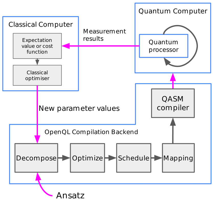

In the first compile run, any parameterised quantum instructions without a numerical value are skipped by any compiler passes that require that specific value. Mapping and scheduling one (or a set of) instruction cannot be done when the qubit is not specified, but do not require knowledge of the angle of a rotation gate. When recompiling, only parameterised quantum instructions and affected instructions are considered, while the rest of the code is left unaffected. This might mean some optimisations that affect large regions of the code will not be done, but this effect is expected to be small compared to the resources saved by not checking all of the code after each compilation.
5.2 Implementation example
An example for how parameters can be used is shown below:
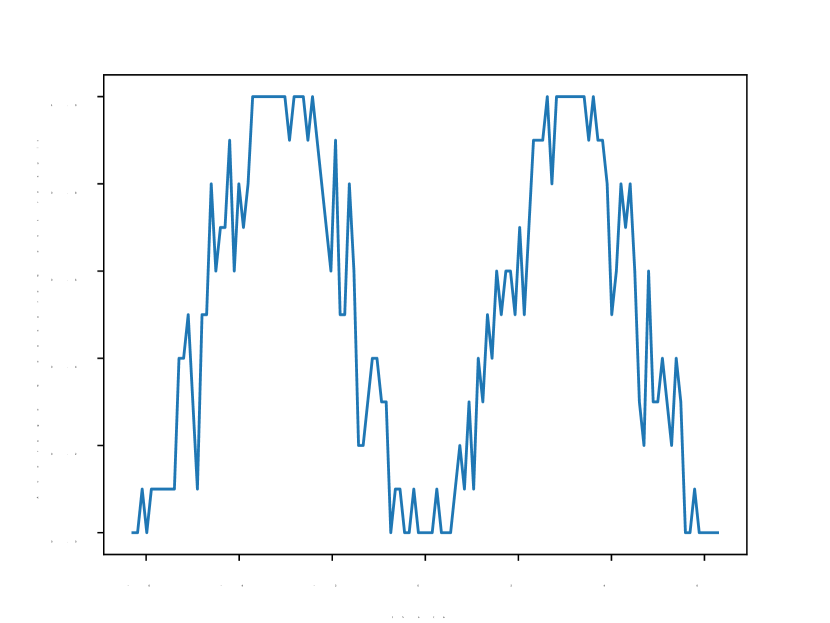
The quantum program in this example is just a single rz gate with parameterised gate angle theta, which is applied to qubit 0. The program is compiled in a for-loop, for the range of angles specified in theta_range on line 9.
When this code is run multiple times, the average measurement result for each angle theta is shown in Fig. 4.
6 Methods
To determine the influence of parameters, execution time tests were performed. These were done with the MAXCUT benchmark [16].
6.1 The MAXCUT benchmark
MAXCUT is a hybrid algorithm which can be used for circuit layout design [2], statistical physics and more [24]. It aims to find the division of a graph into two parts, where the total weight of all edges between the parts is maximised [24]. The general case is an NP-hard problem.
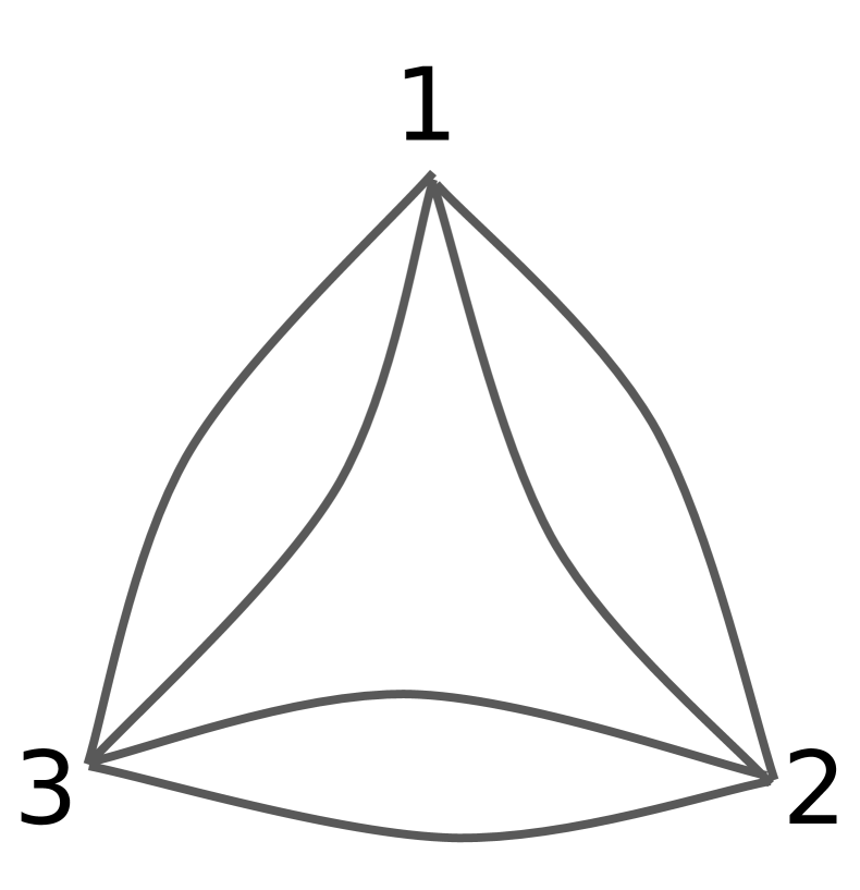
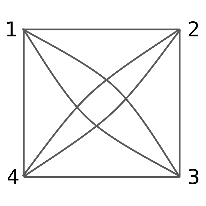
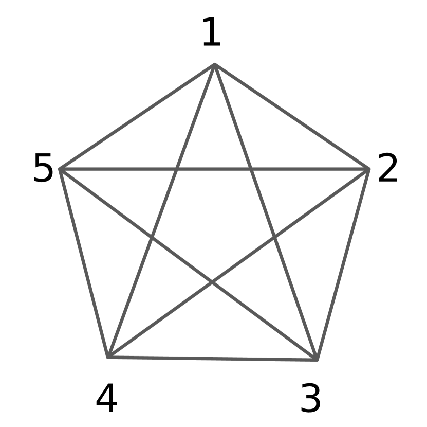
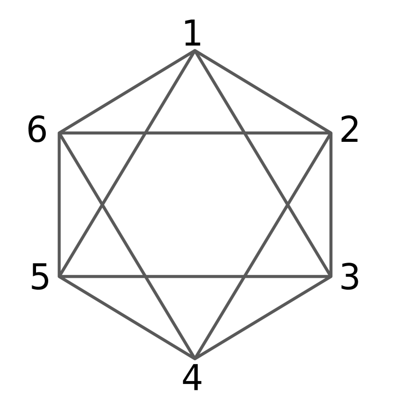
The MAXCUT benchmark from [16] was implemented in OpenQL, PyQuil and Qiskit on 4-regular graphs of varying number of nodes, which are shown in Fig. 5. These graphs and this benchmark were chosen because a reference implementation was already available, it can be easily scaled up to any number of nodes and the number of qubits and the circuit depth both increase linearly with an increasing number of nodes.
The MAXCUT benchmark is a variational quantum algorithm, with an execution flow as in Section 2.1. The quantum circuit for the benchmark consists of the following:
-
•
For a graph with nodes, qubits
-
•
A hadamard gate on each qubit
-
•
Unitary operator consisting of:
-
–
For every edge between between nodes and , a CNOT gate from qubit to
-
–
A on qubit
-
–
Another cnot gate from qubit to
-
–
-
•
Unitary operator consisting of:
-
–
A gate on every qubit
-
–
-
•
Measurement of every qubit
The example below shows the circuit for the MAXCUT benchmark on a graph of two nodes, and , with a single line between them.
| \Qcircuit@C=1em @R=.7em \push | ||||||||
| \push | \ustickp | |||||||
| \push | \lstick|a⟩ | \gateH | \ctrl1 | \qw | \ctrl1 | \qw | \gateR_x(β) | \meter |
| \push | \lstick|b⟩ | \gateH | \targ | \gateR_z(γ) | \targ | \qw | \gateR_x(β) | \meter\gategroup34461.2em– \gategroup38481em– \gategroup34482em^} |
| \dstickU(γ) | \dstickU(β) | |||||||
| \push |
The unitary operators can be repeated for steps as . Increasing the number of these steps improves the quality of the approximation [7]. The total number of gates (excluding measurement) is , for qubits and steps. For our tests, we have chosen to go with steps, which matches the number of steps in the benchmark.
6.2 Experimental setup
In order to compare the performance of OpenQL with other programming languages, the MAXCUT algorithm was implemented in OpenQL and also in Qiskit (0.37.0) and PyQuil (3.1.0). Timing was done from the host Python program using the "time" package, on a Dell Latitude 7400 with an 8th Generation Intel Core™ i7-8665U Processor and 2x 4GiB DDR4 RAM.
To compare the compilation times of OpenQL, OpenQL and Qiskit, a quantum circuit was generated as in Section 6.1. To limit the influence of other factors on the measurement results, the angles for each iteration were not generated using a classical optimiser, but randomly generated outside of the timing loop. The number of steps was set at 3, as mentioned before, and the number of nodes at 15. This corresponds to a circuit with a total of 330 CNOTs and rotation gates, and 15 measurement operators. For each measurement, the language (OpenQL, OpenQL or Qiskit) and the total number of iterations are randomly selected. The compile time is measured from the start of any language-specific preamble and until all iterations have completed. For the iterations a simple loop is used that compiles the circuit with different angle values for the parameters.
Timing was done for a total of 1, 2, 4, 6, 8, 10, 12, 14 and 16 iterations, with and without writing of quantum assembly language to an output file. Although the circuit that is used in these tests comes from the MAXCUT benchmark, no classical optimiser is used for this set of tests. This way, the number of iterations is not dependent on any unknown factors, and the compilation time does not include the runtime of the optimiser. The Qiskit optimisation level was set to 1, which corresponds "light optimisation" [19]. For OpenQL, the "RotationOptimizer" pass was added to the compiler.
To determine whether the improvements made had an impact on any real applications, a full implementation of MAXCUT was used. The circuit and the parameters are the same as in the previous set of tests, but now a classical optimiser was added to the loop to determine the parameter values for the next iteration. The circuits were also run on a simulator, and the measurement results coming from the simulator are used as input for the optimiser. This makes the total execution flow as in Fig. 1. The tests were performed for regular graphs with between 3 and 8 nodes, with 3 steps to the algorithm as before. Tests were performed interleaved where possible, and number of nodes was randomised for each trial. For each run of the MAXCUT benchmark, the number of function evaluations was limited to 100, and any runs that reached convergence earlier where discarded. Therefore the total number of function evaluations for each language is 100, although the number of circuit compilations and simulations can be lower. This is because the loop is aborted preemptively if the optimiser generates negative angles or angles bigger than 2. The effect this has on the results is expected to be small, and it should be the same for each language so does not influence the comparisons made.
7 Results
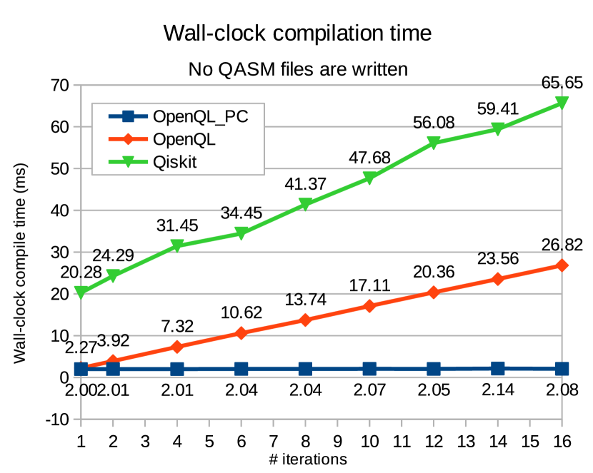
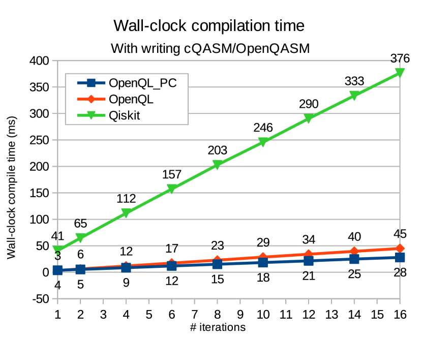
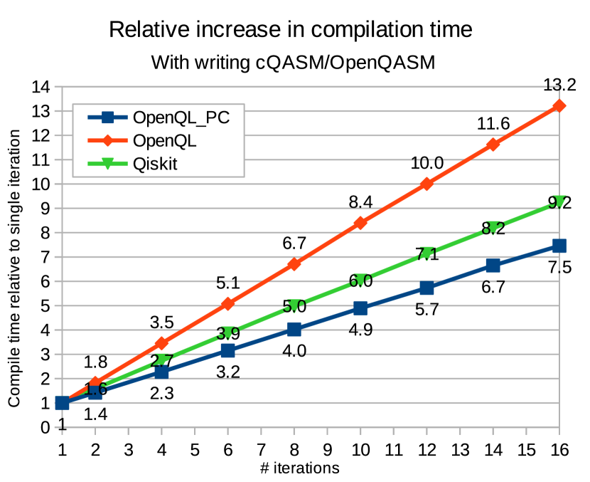
The results for the first set of tests outlined in Section 6.2 (without classical optimiser) can be found in Figs. 6 and 7. Figs. 6 and 7(a) show the wall-clock time in seconds that it cost to compile for the different numbers of iterations. Fig. 7(b) shows these measurements relative to the time of a single iteration (i.e., divided by the time it costs to do just one iteration).
As can be seen in Fig. 6, OpenQL does not perform any additional work beyond the first circuit compilation when there is no QASM output. Therefore, there is (almost) no increase in wall-clock compilation time when the circuit is compiled multiple times. The reason for this is that the parameters are only replaced by their numerical values when they are required, which is only when QASM is generated.
When QASM output is generated, both OpenQL and OpenQL are considerably faster than Qiskit, as can be seen in Fig. 7(a). However, considering the relative increase in compilation times in Fig. 7(b) shows that OpenQL handles repeat compilations worse than either Qiskit or OpenQL, since it is not optimised for this operation. In OpenQL, it takes 13 times as long to do 16 iterations. This is because of setting up the circuit and the compiler, which are done for each iteration instead of only once for the complete run in OpenQL. The time that is saved by OpenQL for subsequent iterations can be seen in both absolute and relative decrease in compile time. OpenQL and OpenQL take almost the same amount of time for a single compilation, but for each subsequent iteration, there is more and more time saved by OpenQL.
Looking at the absolute compile times shows that Qiskit is an overall much slower compiler than OpenQL or OpenQL. Inspecting the relative cost of compiling for multiple iterations, Qiskit shows some level of optimisation for this type of repeated compilations. Still these optimisations are not as effective as the ones implemented in OpenQL, which is faster both in absolute terms and in relative cost of compilation.
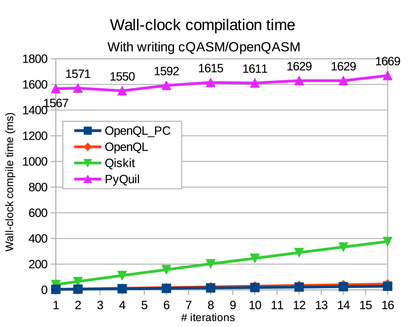
Inspecting the compilation time of PyQuil, Fig. 8 shows that consecutive iterations do not incur much additional time. However, the compile times PyQuil need are 10x to 100x higher than that of the other languages. This is due to the fact that PyQuil has to be compiled by running a separate compiler on a virtual machine in server mode, which are called from the main python program.
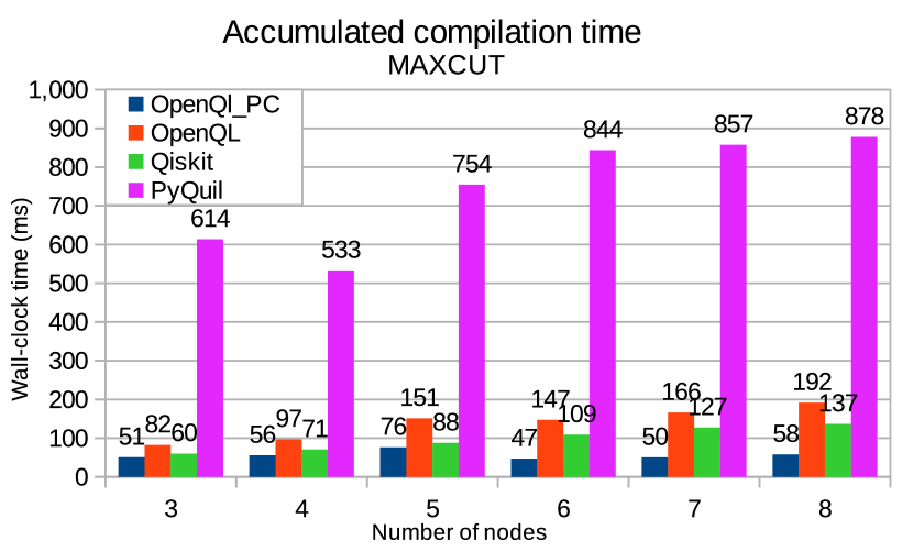
In Fig. 9, we also inspect the accumulated compilation times for running MAXCUT with a classical optimiser for graphs of different numbers of nodes, for OpenQL, OpenQL, Qiskit and PyQuil. OpenQL has the shortest total compile time, second is Qiskit, then OpenQL, and the slowest by an order of magnitude is PyQuil. These benchmark runs were done with fewer nodes and more iterations (namely 100 iterations) than the earlier tests, and it is interesting to see that OpenQL has overtaken Qiskit in compile time. Although Qiskit takes considerably longer to compile a circuit once, as noted before, the time that is saved for each subsequent iteration results in a total shorter time spent compiling. OpenQL combines the already fast compile times of OpenQL with efficiently handling iterations, and as a result is much faster than all other tested options.
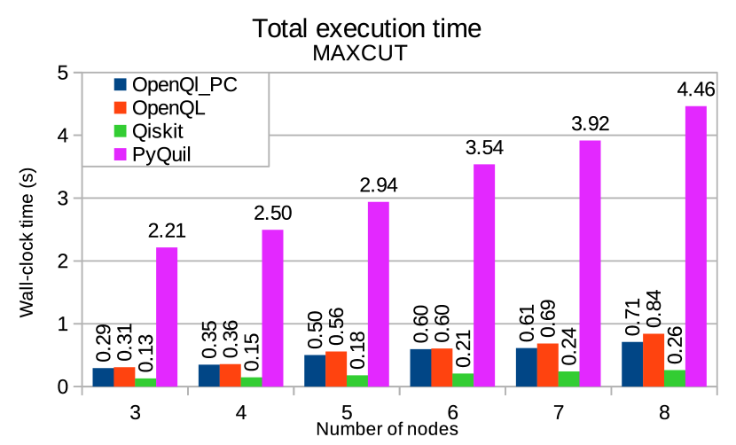
Fig. 10 shows the total execution time of the MAXCUT benchmark, which includes both compilation time as well as simulation time. The figure shows that total execution times are up to 50x higher than compilation times (Fig. 9). Therefore, a big part of the difference in execution time between the programming languages is due to the difference in performance between the corresponding simulators. Still, the same trend can be seen, where PyQuil takes the longest time by far, and both OpenQL and OpenQL have similar performance, since OpenQL and OpenQL both use the QX simulator. The figure also shows that the Qiskit Aer simulator is the fastest of the tested options.
In summary, the results show that the improvements made for OpenQL result in a clear speedup compared to OpenQL. Compared to Qiskit and PyQuil, OpenQL has the fastest compile times for the MAXCUT benchmark. However, when looking at the total execution time, the fast simulator time of Qiskit Aer results in the shortest total execution time of the benchmark. This can be partly explained by the large communication time between OpenQL/OpenQL and the QX simulator, which requires writing and reading of a QASM file for every iteration. This is especially apparent in the MAXCUT benchmark, which has a lot of iterations for relatively short circuits, which results in a lot of read/write operations compared to circuit compilation(s). Between the Qiskit compiler and the Qiskit Aer simulator, however, the circuit can be passed directly.
8 Conclusion
In this paper, we introduced OpenQL, an efficient approach to parametric compilation for hybrid quantum-classical algorithms, and implemented it in the OpenQL programming framework. OpenQL is designed to be modular, scalable, usable, future-proof and fast. We compared wall-clock compilation time of OpenQL with OpenQL, Qiskit and PyQuil. The total compilation time was measured using the MAXCUT benchmark from [16].
Experimental results show that compared to other programming languages, total compile time of OpenQL and OpenQL is between 10 and 20 times faster than Qiskit, respectively. PyQuil had the slowest time at about 60x slower than OpenQL. In addition, comparing compile times of multiple compile iterations relative to single iterations shows that OpenQL is the fastest, followed by Qiskit which is 1.2x slower, while OpenQL took the most time being 1.8x slower than OpenQL.
The MAXCUT benchmark was also implemented in its entirety, including a classical optimiser and simulations. These tests, with shorter circuits but more iterations than before, show that the improvements made in OpenQL result in a decrease of 40 to 70% in (accumulated) compilation time. This makes OpenQL faster than all other tested languages. For the total execution (run)time of the MAXCUT benchmark, the performance of the simulators used has more influence than the compile times of the languages. The simulator used with PyQuil is still the slowest option by far, but the Qiskit Aer simulator is 2 to 3 times as fast as the QX simulator used by OpenQL and OpenQL. Even so, the faster compile time of OpenQL does lead to some speed-up of the complete benchmark.
It is important to note that the measurements of the complete MAXCUT benchmark show that when simulating quantum algorithms on classical computers, the simulation time can be excessively large as expected, which limits the impact of the improvement achieved by our approach. However, the impact of our approach becomes significant when running these algorithms on real quantum devices. Furthermore, a single compilation of a quantum circuit is projected to become more computationally expensive as more sophisticated mapping, optimisation and error-correcting algorithms are created and implemented, which will further increase the cost of repeated compilations in hybrid algorithms and increase the impact of our approach.
References
- [1] Frank Arute et al. “Quantum Supremacy using a Programmable Superconducting Processor” In Nature 574, 2019, pp. 505–510 URL: https://www.nature.com/articles/s41586-019-1666-5
- [2] Francisco Barahona, Martin Grötschel, Michael Jünger and Gerhard Reinelt “An Application of Combinatorial Optimization to Statistical Physics and Circuit Layout Design” In Oper. Res. 36, 1988, pp. 493–513
- [3] Sergio Boixo et al. “Characterizing quantum supremacy in near-term devices” In Nature Physics 14.6 Springer ScienceBusiness Media LLC, 2018, pp. 595–600 DOI: 10.1038/s41567-018-0124-x
- [4] Frederic Chong and Margaret Martonosi “Programming languages and compiler design for realistic quantum hardware” In Nature 549, 2017, pp. 180–187 DOI: 10.1038/nature23459
- [5] Rigetti Computing “PyQuil documention”, 2021 URL: https://pyquil-docs.rigetti.com/en/stable
- [6] Suguru Endo, Zhenyu Cai, Simon C. Benjamin and Xiao Yuan “Hybrid Quantum-Classical Algorithms and Quantum Error Mitigation” In Journal of the Physical Society of Japan 90.3, 2021, pp. 032001 DOI: 10.7566/JPSJ.90.032001
- [7] Edward Farhi, Jeffrey Goldstone and Sam Gutmann “A Quantum Approximate Optimization Algorithm”, 2014 arXiv:1411.4028 [quant-ph]
- [8] Harper R. Grimsley, Sophia E. Economou, Edwin Barnes and Nicholas J. Mayhall “An adaptive variational algorithm for exact molecular simulations on a quantum computer” In Nature Communications 10.1 Springer ScienceBusiness Media LLC, 2019 DOI: 10.1038/s41467-019-10988-2
- [9] Lov K. Grover “A fast quantum mechanical algorithm for database search” arXiv, 1996 DOI: 10.48550/ARXIV.QUANT-PH/9605043
- [10] Abhinav Kandala et al. “Hardware-efficient variational quantum eigensolver for small molecules and quantum magnets” In Nature 549.7671 Springer ScienceBusiness Media LLC, 2017, pp. 242–246 DOI: 10.1038/nature23879
- [11] Peter J Karalekas et al. “A quantum-classical cloud platform optimized for variational hybrid algorithms” In Quantum Science and Technology 5.2 IOP Publishing, 2020, pp. 024003 DOI: 10.1088/2058-9565/ab7559
- [12] N. Khammassi et al. “OpenQL : A Portable Quantum Programming Framework for Quantum Accelerators”, 2020 arXiv:2005.13283 [quant-ph]
- [13] Nader Khammassi et al. “QX: A high-performance quantum computer simulation platform” Design, Automation and Test in Europe : DATE 17 ; Conference date: 27-03-2017 Through 31-03-2017 In Proceedings of the 2017 Design, Automation & Test in Europe Conference & Exhibition (DATE) United States: IEEE, 2017, pp. 464–469 DOI: 10.23919/DATE.2017.7927034
- [14] Jin-Guo Liu, Yi-Hong Zhang, Yuan Wan and Lei Wang “Variational quantum eigensolver with fewer qubits” In Physical Review Research 1.2 American Physical Society (APS), 2019 DOI: 10.1103/physrevresearch.1.023025
- [15] Jarrod R McClean, Jonathan Romero, Ryan Babbush and Alán Aspuru-Guzik “The theory of variational hybrid quantum-classical algorithms” In New Journal of Physics 18.2 IOP Publishing, 2016, pp. 023023 DOI: 10.1088/1367-2630/18/2/023023
- [16] Koen Mesman, Zaid Al-Ars and Matthias Möller “QPack: Quantum Approximate Optimization Algorithms as universal benchmark for quantum computers” In CoRR abs/2103.17193, 2021 arXiv: https://arxiv.org/abs/2103.17193
- [17] Aidan Pellow-Jarman, Ilya Sinayskiy, Anban Pillay and Francesco Petruccione “A Comparison of Various Classical Optimizers for a Variational Quantum Linear Solver”, 2021
- [18] Alberto Peruzzo et al. “A variational eigenvalue solver on a photonic quantum processor” In Nature Communications 5.1 Springer ScienceBusiness Media LLC, 2014 DOI: 10.1038/ncomms5213
- [19] Qiskit Development team “Qiskit documentation” Accessed on: 10-07-2020, 2020 URL: https://qiskit.org/documentation/
- [20] Aritra Sarkar, Zaid Al-Ars and Koen Bertels “QuASeR: Quantum Accelerated de novo DNA sequence reconstruction” In PLOS ONE 16.4 Public Library of Science, 2021, pp. 1–23 DOI: 10.1371/journal.pone.0249850
- [21] P.W. Shor “Algorithms for quantum computation: discrete logarithms and factoring” In Proceedings 35th Annual Symposium on Foundations of Computer Science, 1994, pp. 124–134 DOI: 10.1109/SFCS.1994.365700
- [22] Robert Smith et al. “Pyquil: Quantum programming in Python” Accessed on: 24-06-2020, 2020 URL: https://github.com/rigetti/pyquil
- [23] Robert S. Smith, Michael J. Curtis and William J. Zeng “A Practical Quantum Instruction Set Architecture”, 2016 arXiv:1608.03355 [quant-ph]
- [24] Rui-Sheng Wang and Li-Min Wang “Maximum cut in fuzzy nature: Models and algorithms” In Journal of Computational and Applied Mathematics 234.1, 2010, pp. 240–252 DOI: https://doi.org/10.1016/j.cam.2009.12.022