Accurate localization of Kosterlitz-Thouless-type quantum phase transitions
for one-dimensional spinless fermions

Abstract

We investigate the charge-density wave (CDW) transition for one-dimensional spinless fermions at half band-filling with nearest-neighbor electron transfer amplitude $t$ and interaction $V$. The model is equivalent to the anisotropic XXZ Heisenberg model for which the Bethe Ansatz provides an exact solution. For $V>V_{\rm c}=2t$, the CDW order parameter and the single-particle gap are finite but exponentially small, as is characteristic for a Kosterlitz-Thouless transition. It is notoriously difficult to locate such infinite-order phase transitions in the phase diagram using approximate analytical and numerical approaches. Second-order Hartree-Fock theory is qualitatively applicable for all interaction strengths, and predicts the CDW transition to occur at $V_{\rm c,2}^{(2)}\approx 1.5t$. Second-order Hartree Fock theory is almost variational because the density of quasi-particle excitations is small. We apply the density-matrix renormalization group (DMRG) for periodic boundary conditions for system sizes up to 514 sites which permits a reliable extrapolation of all physical quantities to the thermodynamic limit, apart from the critical region. We investigate the ground-state energy, the gap, the order parameter, the momentum distribution, the quasi-particle density, and the density-density correlation function to locate $V_{\rm c}$ from the DMRG data. Tracing the breakdown of the Luttinger liquid and the peak in the quasi-particle density at the band edge permits us to reproduce $V_{\rm c}$ with an accuracy of one percent.

I Introduction

The isotropic spin-1/2 Heisenberg model on a chain was the first exactly solved many-body problem. Bethe (1931) Three decades later, Orbach, Orbach (1958) and later Yang and Yang,  Yang and Yang (1966a, b) succeeded to generalize the Bethe Ansatz to the one-dimensional anisotropic Heisenberg (or XXZ) model,

$$\hat{H}_{\rm XXZ}(\Delta)=-\frac{1}{2}\sum_{l=1}^{L-1}\Bigl{[}\underline{\underline{\sigma}}_{l}^{x}\cdot\underline{\underline{\sigma}}_{l+1}^{x}+\underline{\underline{\sigma}}_{l}^{y}\cdot\underline{\underline{\sigma}}_{l+1}^{y}+\Delta\underline{\underline{\sigma}}_{l}^{z}\cdot\underline{\underline{\sigma}}_{l+1}^{z}\Bigr{]}\;,$$ (1)

where $\underline{\underline{\sigma}}_{l}^{x,y,z}$ are the Pauli matrices on site $l$ and $\Delta\leq 0$ is the anisotropy parameter for antiferromagnetic coupling. The XXZ model reduces to the Ising model in the limit of strong anisotropy in the $z$-direction, $|\Delta|\to\infty$. Since the 1960s, many exact results for the model in the thermodynamic limit were established, e.g., the ground-state energy, Yang and Yang (1966a, b) the elementary spinon excitations, Johnson et al. (1973); Babelon et al. (1983); Woynarovich (1982); Virosztek and Woynarovich (1984) and the staggered magnetization in the Ising regime, $|\Delta|\geq 1$, Baxter (1973); Izergin et al. (1999) to name a few. An efficient exact description of the thermodynamic properties was achieved by Klümper. Klümper (1993)

Starting from the early 1990s Jimbo et al. (1992) the focus of the exact calculations shifted to the reduced density matrix which was fully characterized in the following decade. Jimbo and Miwa (1996); Kitanine et al. (2000); Göhmann et al. (2005); Boos et al. (2009); Jimbo et al. (2009); Boos and Göhmann (2009) This made it possible to derive a number of spin correlation functions analytically, see, e.g., Refs. [Bortz and Göhmann, 2005; Damerau et al., 2007; Boos et al., 2008]. Most recently, fully explicit series representations for the exact dynamical spin correlation functions and the spin conductivity were obtained in the Ising regime. Babenko et al. (2021); Göhmann et al. (2022) Therefore, the XXZ model belongs to the best studied and understood many-particle systems.

Via a Jordan-Wigner transformation, the antiferromagnetic XXZ model on a chain with $\Delta\leq 0$ and zero magnetization maps onto a model for spinless fermions with open boundary conditions at half band-filling with nearest-neighbor electron transfer amplitude $(-t)$ and repulsive interaction $V=-\Delta/(2t)\geq 0$. Jordan and Wigner (1928) While the XXZ model contains a transition to an antiferromagnetically ordered ground state at the Heisenberg point, $\Delta=-1$, the model for spinless fermions displays a metal-insulator transition at $V_{\rm c}=2t$ from a Luttinger liquid to a charge-density wave (CDW) insulator.

A transition at finite interaction strength is unexpected because the nesting instability would place the transition at $V_{\rm c}^{\rm(1)}=0^{+}$, and it requires a sophisticated renormalization group treatment to show that the system is marginally stable against the formation of a CDW at weak coupling. Di Castro and Metzner (1991); Shankar (1994) The same result can be obtained using bosonization, see Ref. [Giamarchi, 2004] for an introduction. To complicate matters, the single-particle gap and the order parameter display an essential singularity at $V_{\rm c}$, i.e., they open exponentially as a function of $1/\sqrt{V-V_{\rm c}}$, as is characteristic for a Kosterlitz-Thouless transition. Kosterlitz and Thouless (1973) Consequently, it is notoriously difficult to determine the critical interaction strength for the transition using approximate analytical and numerical approaches. Transitions of Kosterlitz-Thouless type are common in one-dimensional quantum systems such as in the bosonic Hubbard model, see e.g., Ref. [Kühner et al., 2000], or quantum spin chains, see, e.g., Ref. [Montenegro-Filho et al., 2020].

Since spinless fermions represent a rare case of an exactly solvable model with a metal-insulator transition at a finite interaction strength, it is desirable to see if and how well approximate methods are able to reproduce the formation of CDW order at $V_{\rm c}=2t$. As our analytical approximations we use Hartree-Fock theory and second-order perturbation theory around it. Georges and Yedidia (1991); van Dongen (1994) First-order Hartree-Fock theory suggests a CDW for all finite interaction strengths, $V_{\rm c}^{\rm(1)}=0^{+}$, corresponding to the nesting instability. As we shall show in this work, second-order Hartree-Fock approximation predicts a discontinuous transition at $V_{\rm c,2}^{(2)}\approx 1.5$ with a jump in the order parameter and concomitant discontinuities in physical quantities.

As numerical approach, we employ the density-matrix renormalization group (DMRG) method White (1992, 1993); Schollwöck (2005) that provides highly accurate data for finite rings with up to $L=514$ sites; we choose periodic boundary conditions and even $L/2$ for an open-shell ground state to reduce finite-size effects. To make contact with finite-size corrections calculated for the XXZ model from Bethe Ansatz, we also investigate odd $L/2$.

We identify two successful strategies to locate accurately the CDW transition. The first route monitors the breakdown of the metallic phase. The properties of the Luttinger liquid are reflected in finite-size corrections to the ground-state energy and the gap, and most prominently in the Luttinger parameter that determines the momentum distribution close to the Fermi points and the small-momentum limit of the density-density correlation function. In the end, the accurate calculation of the Luttinger parameter permits to locate the breakdown of the Luttinger liquid with an accuracy of three percent. Following an alternative route, we trace the maximum of the quasi-particle distribution as a function of system size and interaction. Using this independent approach, we determine the critical interaction strength with an accuracy of one percent.

The paper is organized as follows. In Sect. II we define the model Hamiltonian for spinless fermions. We discuss its relation to the XXZ model for various boundary conditions and particle numbers.

In Sect. III we put together exact results from the literature for the ground-state energy, the nearest-neighbor single-particle density matrix, the single-particle gap, and the charge-density wave order parameter in the thermodynamic limit. Since this information is often phrased for the XXZ model and is not summarized in reviews or books, we find it useful to compose them here for spinless fermions. Limiting cases are derived and discussed in the supplemental material sup (see, also, references [Banerjee and Wilkerson, 2017; Garoufalidis and Zagier, 2021] therein).

In Sect. IV we present the standard (first-order) Hartree-Fock approximation for spinless fermions. This permits us to introduce the lower and upper Hartree-Fock bands in the reduced Brillouin zone and the corresponding quasi-particle operators.

In Sect. V we calculate the second-order weak-coupling perturbation correction to the Hartree-Fock approximation, and justify its applicability to all interaction strengths. Technicalities for the second-order Hartree-Fock calculations can be found in the supplemental material. sup

In Sect. VI we compare approximate results with those from the exact Bethe-Ansatz solutions. We focus on the issue how to obtain the critical interaction strength for the charge-density wave transition from finite-size DMRG data.

Short conclusions, Sect. VII, close our presentation.

II Spinless fermions in one dimension

We start with the introduction of the Hamiltonian for spinless fermions and discuss its relation to the XXZ Heisenberg model.

II.1 Hamiltonian

The Hamiltonian for spinless fermions on a ring with $L$ lattice sites reads

$$\hat{H}=\hat{T}+\hat{V}\;.$$ (2)

The kinetic energy operator describes the transfer of fermions between neighboring sites with real amplitude $(-t)$ and $t>0$

$$\hat{T}=(-t)\sum_{l=1}^{L}\left(\hat{c}_{l+1}^{+}\hat{c}_{l}^{\vphantom{+}}+\hat{c}_{l}^{+}\hat{c}_{l+1}^{\vphantom{+}}\right)\;,$$ (3)

where $\hat{c}_{l}^{+}$ ($\hat{c}_{l}^{\vphantom{+}}$) creates (annihilates) a fermion on lattice site $l$, $l=1,2,\ldots,L$; we choose $L/2$ to be even if not stated explicitly otherwise. Periodic boundary conditions apply, $\hat{c}_{L+l}\equiv\hat{c}_{l}$. The nearest-neighbor interaction with strength $V$ is given by

$$\hat{V}=V\sum_{l=1}^{L}\hat{n}_{l}\hat{n}_{l+1}\;,$$ (4)

where $\hat{n}_{l}=\hat{c}_{l}^{+}\hat{c}_{l}^{\vphantom{+}}$ counts the number of fermions on site $l$, and $V>0$ is repulsive.

The kinetic energy is diagonal in momentum space using the Fourier transformation

$$\hat{a}_{k} = \sqrt{\frac{1}{L}}\sum_{l=1}^{L}e^{-{\rm i}kl}\hat{c}_{l}\;,$$ (5)

$$\hat{c}_{l} = \sqrt{\frac{1}{L}}\sum_{k}e^{{\rm i}kl}\hat{a}_{k}\;,$$ (6)

where $k=(2\pi/L)m$, $m=-L/2,-L/2+1,\ldots,L/2-1$, to fulfill periodic boundary conditions. We have

$$\hat{T}=\sum_{k}\epsilon(k)\hat{a}_{k}^{+}\hat{a}_{k}^{\vphantom{+}}\;,\quad\epsilon(k)=-2t\cos(k)\;.$$ (7)

In the following we shall focus on the case of half band-filling, where the number of fermions $N$ equals half the number of lattice sites, $N=L/2$, and use $t\equiv 1$ as our energy unit. The bare bandwidth is $W=4$.

II.2 XXZ Heisenberg model

The model for spinless fermions in one dimension can be transformed into the XXZ Heisenberg model using a Jordan-Wigner transformation. For the moment, let us assume open boundary conditions. On a chain, the XXZ model is given by eq. (1). Using spin operators,

$$\hat{S}_{l}^{x,y,z} = \frac{1}{2}\underline{\underline{\sigma}}_{l}^{x,y,z}\;,$$

$$\hat{S}_{l}^{+} = \hat{S}_{l}^{x}+{\rm i}\hat{S}_{l}^{y}\;,$$

$$\hat{S}_{l}^{-} = \hat{S}_{l}^{x}-{\rm i}\hat{S}_{l}^{y}\;,$$ (8)

the XXZ Heisenberg model reads

$$\hat{H}_{\rm XXZ}(\Delta)=-\sum_{l=1}^{L-1}\left[\hat{S}_{l}^{+}\hat{S}_{l+1}^{-}+\hat{S}_{l+1}^{+}\hat{S}_{l}^{-}\right]-2\Delta\sum_{l=1}^{L-1}\hat{S}_{l}^{z}\hat{S}_{l+1}^{z}\,.$$ (9)

Note that spin operators on different lattice sites commute with each other.

The Pauli particle operators

$$\hat{b}_{l}^{+} = \hat{S}^{+}_{l}\;,$$

$$\hat{b}_{l}^{\vphantom{+}} = \hat{S}_{l}^{-}\;,$$

$$\hat{n}^{b}_{l} = \hat{b}_{l}^{+}\hat{b}_{l}^{\vphantom{+}}=\hat{S}_{l}^{z}+\frac{1}{2}$$ (10)

obey fermionic anticommutation relations between operators on the same site but bosonic commutation relations between different sites. This deficiency is cured by the Jordan-Wigner transformation, Jordan and Wigner (1928); Lieb et al. (1961)

$$\hat{c}_{l}^{+} = \exp\left({\rm i}\pi\sum_{k=1}^{l-1}\hat{n}_{k}^{b}\right)\hat{b}_{l}^{+}\;,$$

$$\hat{c}_{l}^{\vphantom{+}} = \exp\left(-{\rm i}\pi\sum_{k=1}^{l-1}\hat{n}_{k}^{b}\right)\hat{b}_{l}^{\vphantom{+}}\;,$$

$$\hat{n}_{l} = \hat{c}_{l}^{+}\hat{c}_{l}^{\vphantom{+}}=\hat{b}_{l}^{+}\hat{b}_{l}^{\vphantom{+}}=\hat{n}_{l}^{b}\;.$$ (11)

Therefore, the XXZ Heisenberg model can be written in terms of spinless fermions as

$$\hat{H}_{\rm XXZ}(\Delta) = -\sum_{l=1}^{L-1}\left(\hat{c}_{l}^{+}\hat{c}_{l+1}^{\vphantom{+}}+\hat{c}_{l+1}^{+}\hat{c}_{l}^{\vphantom{+}}\right)$$ (12)

$$-2\Delta\sum_{l=1}^{L-1}\left(\hat{n}_{l}-\frac{1}{2}\right)\left(\hat{n}_{l+1}-\frac{1}{2}\right)$$

when open boundary conditions are employed. Thus, the equivalence reads

$$\hat{H}_{\rm XXZ}(-V/2)=\hat{H}(V)-V\hat{N}+V\frac{L}{4}\;.$$ (13)

Eq. (13) permits to translate exact results for the antiferromagnetic XXZ model $\hat{H}_{\rm XXZ}(\Delta\leq 0)$ to the model of spinless fermions for $V\geq 0$ for open boundary conditions.

For the case of periodic boundary conditions, an additional boundary term arises, Lieb et al. (1961)

$$\hat{H}_{\rm XXZ}^{\rm pbc}(\Delta) = -\sum_{l=1}^{L}\left(\hat{c}_{l}^{+}\hat{c}_{l+1}^{\vphantom{+}}+\hat{c}_{l+1}^{+}\hat{c}_{l}^{\vphantom{+}}\right)$$ (14)

$$-2\Delta\sum_{l=1}^{L}\left(\hat{n}_{l}-\frac{1}{2}\right)\left(\hat{n}_{l+1}-\frac{1}{2}\right)$$

$$+\left(\hat{c}_{L}^{+}\hat{c}_{1}^{\vphantom{+}}+\hat{c}_{1}^{+}\hat{c}_{L}^{\vphantom{+}}\right)\left(\exp({\rm i}\pi\hat{N})+1\right)\,.\;$$

Therefore, a comparison of Bethe Ansatz results for the periodic XXZ model with those for spinless fermions on a ring are only possible in the thermodynamic limit, or, when finite-size corrections are addressed, for situations where the particle number $N$ is odd. For the ground state at half band-filling it implies that $L/2$ must be odd. For excitations from the half-filled ground state we must study the sector with two particle or two hole excitations, $N=L/2\pm 2$.

III Exact results

In this section we collect exact results in the thermodynamic limit for the ground-state energy and the nearest-neighbor single-particle density matrix at half band-filling, the single-particle gap, the charge-density wave order parameter, the correlation energy, the momentum distribution, and the density-density correlation function.

III.1 Ground-state energy and nearest-neighbor single-particle density matrix at half band-filling

In the sector of half band-filling we have $N=L/2$ so that eq. (13) gives

$$e_{0}(V)=e_{0}^{\rm XXZ}(-V/2)+\frac{V}{4}$$ (15)

for the energy per lattice site in the thermodynamic limit, $N,L\to\infty$, $N/L=1/2$, where $e_{0}^{\rm XXZ}(\Delta)$ is the energy per lattice site in the XXZ model with antiferromagnetic anisotropy and zero magnetization.

Yang and Yang Yang and Yang (1966a, b) give the following expressions for the ground-state energy density at zero magnetization ($e_{0}^{\rm XXZ}(\Delta)=2f(\Delta,0)$ in the work of Yang and Yang),

$$e_{0}^{\rm XXZ}(-V/2)=\left\{\begin{array}[]{@{}lcl@{}}g(\mu)&\hbox{for}&V=2\cos(\mu)<2\;,\\[6.0pt] \displaystyle 1/2-2\ln(2)&\hbox{for}&V=2\;,\\[6.0pt] h(\lambda)&\hbox{for}&V=2\cosh(\lambda)>2\;,\end{array}\right.$$ (16)

where

$$g(\mu) = \frac{\cos(\mu)}{2}-\int_{-\infty}^{\infty}\frac{\sin^{2}(\mu){\rm d}x}{\cosh(\pi x)[\cosh(2\mu x)-\cos(\mu)]}\;,$$

$$h(\lambda) = \frac{\cosh(\lambda)}{2}-\frac{\sinh(\lambda)}{\lambda}\left[\lambda+4\lambda\sum_{n=1}^{\infty}\frac{1}{1+\exp(2\lambda n)}\right]\;.$$

The first and the third region can be continuously extended to $V=2$. The above formulae can be expressed in terms of $q$-digamma functions Göhmann (2022) We shall not digress into the representation by special functions here.

Expansions for small and large $V$ can be found in the supplemental material. sup For comparison with Hartree-Fock theory, we give the leading-order results for weak and strong interactions,

$$e_{0}(V\ll 1) = -\frac{2}{\pi}+\left(\frac{1}{4}-\frac{1}{\pi^{2}}\right)V$$

$$+\left(-\frac{2}{3\pi^{3}}+\frac{1}{36\pi}\right)V^{2}\;,$$

$$e_{0}(V\gg 1) = -\frac{1}{V}+\frac{1}{V^{3}}\;.$$ (19)

For more details, see the supplemental material. sup

With the help of the Hellmann-Feynman theorem, Hellmann (2015); Feynman (1939) both the potential energy and the kinetic energy can be derived from the exact ground-state energy,

$$\langle\hat{V}\rangle/L = V\frac{\partial e_{0}(V)}{\partial V}\;,$$

$$\langle\hat{T}\rangle/L = e_{0}(V)-V\frac{\partial e_{0}(V)}{\partial V}\;.$$ (20)

Since there is no bond-order wave in the exact ground state, the kinetic energy is just a multiple of the nearest-neighbor single-particle density matrix,

$$B_{0}=-\frac{1}{2L}\langle\hat{T}\rangle=-\frac{1}{2}\left(e_{0}(V)-V\frac{\partial e_{0}(V)}{\partial V}\right)\;.$$ (21)

The limiting values are

$$B_{0}(V\ll 1) = \frac{1}{\pi}-\left(\frac{1}{3\pi^{3}}-\frac{1}{72\pi}\right)V^{2}\;,$$

$$B_{0}(V\gg 1) = \frac{1}{V}-\frac{2}{V^{3}}\;.$$ (22)

For more details, see the supplemental material. sup

III.2 Single-particle gap

III.2.1 Particle-hole symmetry

The XXZ Hamiltonian in the fermionic language (12) is particle-hole symmetric so that the chemical potential $\mu=0$ guarantees half filling for all temperatures. To see this, we perform the particle-hole transformation

$$\tau_{\rm ph}:\quad\hat{c}_{l}^{\vphantom{+}}\to(-1)^{l}\hat{c}_{l}^{+}\quad,\quad\hat{a}_{k}^{\vphantom{+}}\to\hat{a}_{k+\pi}^{+}$$ (23)

that leaves the Hamiltonian $\hat{H}_{\rm XXZ}$ in eq. (12) invariant but changes the particle number operator, $\hat{N}\to L-\hat{N}$. Therefore,

$$\langle\hat{N}\rangle^{\rm XXZ}(T,V,\mu=0) = \frac{1}{Z}\mathop{\rm Tr}\left\{e^{-\beta\hat{H}_{\rm XXZ}}\hat{N}\right\}$$ (24)

$$= \frac{1}{Z}\mathop{\rm Tr}\left\{e^{-\beta\hat{H}_{\rm XXZ}}\left(L-\hat{N}\right)\right\}$$

$$= L-\langle\hat{N}\rangle^{\rm XXZ}(T,V,\mu=0)$$

so that $\mu=0$ indeed guarantees half band-filling for all temperatures $T=1/\beta$ and interaction strengths $V$, $\langle\hat{N}\rangle^{\rm XXZ}(T,V,\mu=0)=L/2$.

At zero temperature, the energies for adding another fermion to the half-filled system and adding a particle to reach half filling are given by

$$\mu_{1}^{+}(V) = E_{0}(L/2+1,V)-E_{0}(L/2,V)\;,$$

$$\mu_{1}^{-}(V) = E_{0}(L/2,V)-E_{0}(L/2-1,V)\;.$$ (25)

The chemical potentials define the gap at half filling,

$$\Delta_{1}(V) = \mu_{1}^{+}(V)-\mu_{1}^{-}(V)$$ (26)

$$= \mu_{1}^{+,{\rm XXZ}}(-V/2)-\mu_{1}^{-,{\rm XXZ}}(-V/2)$$

$$= 2\mu_{1}^{+,{\rm XXZ}}(-V/2)$$

$$= 2(\mu_{1}^{+}(V)-V)\;,$$

where we used particle-hole symmetry in the next to last step,

$$E_{0}^{\rm XXZ}(L-N,V)=E_{0}^{\rm XXZ}(N,V)$$ (27)

for the ground-state energy with $N$ and $L-N$ fermions. Due to eq. (26), we only need to calculate the ground-state energy at half band-filling and with one additional fermion to calculate the single-particle gap $\Delta_{1}(V)$, or with two additional particles when we calculate the two-particle gap $\Delta_{2}(V)$.

For the momentum distribution,

$$n_{k}=\langle\hat{a}_{k}^{+}\hat{a}_{k}^{\vphantom{+}}\rangle\;,$$ (28)

it is sufficient to investigate the region $|k|\leq\pi/2$ because particle-hole symmetry leads to

$$n_{k}=1-n_{k\pm\pi}$$ (29)

when $|k|>\pi/2$ and periodic boundary conditions are employed.

III.2.2 Gap formula from the XXZ model

In the antiferromagnetic XXZ model, the elementary excitations are spin-1/2 objects called spinons. For a spin-flip in the XXZ model, (at least) two spinons are required. Adding or subtracting a particle in the model for spinless fermions corresponds to such a spin flip. Since the spinon dispersion is gapped for $\Delta<-1$, there is a finite gap for charge excitations for $V>V_{\rm c}=2$.

The spinon dispersion for the XXZ chain is known analytically, Johnson et al. (1973); Babelon et al. (1983) (recall $\Delta=-V/2$)

$$\epsilon_{s}(p,V) = \frac{2K(m)}{\pi}\sinh(\gamma)\sqrt{1-m\cos^{2}(p)}\;,$$

$$\cosh(\gamma) = \frac{V}{2}\;,\quad 0\leq p\leq\pi\;.$$ (30)

Here, $K(m)$ is the complete elliptic integral of the first kind,

$$K(m)=\int_{0}^{\pi/2}\frac{{\rm d}\theta}{\sqrt{1-m\sin^{2}(\theta)}}\,$$ (31)

and $m$ follows from the solution of the implicit equation

$$\gamma=\frac{\pi K(1-m)}{K(m)}\;.$$ (32)

Since it takes two spinons to create a spin-flip, we have

$$\mu_{1}^{+,{\rm XXZ}}(V)=2\epsilon_{s}(0,V)\;.$$ (33)

Therefore, the single-particle gap is given by

$$\Delta_{1}(V)=\frac{8K(m)}{\pi}\sinh(\gamma)\sqrt{1-m}\;.$$ (34)

The single-particle gap can be expressed more compactly in terms of Jacobi functions. Göhmann (2022)

Analytic results close to the transition and for strong coupling are summarized in the supplemental material. sup For comparison with approximate treatments, we list the leading-order behavior close to the transition and the strong-coupling result,

$$\Delta_{1}(V\gtrsim 2) = 16\pi\exp\left(-\frac{\pi^{2}}{2\sqrt{V-2}}\right)\;,$$ (35)

$$\Delta_{1}(V\gg 1) = 2V-8+\frac{4}{V}\;.$$ (36)

Apparently, above the transition the gap opens exponentially in $1/\sqrt{V-V_{\rm c}}$. A similar exponential behavior is characteristic for the Kosterlitz-Thouless transition in certain two-dimensional models at finite temperature. Kosterlitz and Thouless (1973) Therefore, it is said that the quantum phase transition is of ‘Kosterlitz-Thouless type’.

The result for strong coupling is readily understood. An extra fermion added to the half-filled system leads to three fermions in a row and thus to two nearest-neighbor interactions with an excitation energy of $2V$. The transfer of particles between neighboring sites results in the free motion of domain walls to the right and left. Therefore, the first correction term to the single-particle is twice the bandwidth, namely $W=4$ for each domain wall.

III.3 Order parameter

For spinless fermions, the charge density obeys

$$\langle\hat{n}_{l}\rangle=\frac{1}{2}+(-1)^{l}n_{a}(V)$$ (37)

with $0\leq n_{a}(V)\leq 1/2$ when we select the CDW solution with higher particle density on the even lattice sites. Note that $n_{a}(V)$ is finite for $V>V_{\rm c}=2$ and $n_{a}(V\to\infty)=1/2$ for strong coupling.

The order parameter for the XXZ Heisenberg model in the thermodynamic limit was calculated by Baxter using the Bethe Ansatz,Baxter (1973) and re-derived by Izergin et al. using the algebraic Bethe Ansatz.Izergin et al. (1999) They give

$$s_{0}(q)=\left[\prod_{m=1}^{\infty}\frac{1-q^{2m}}{1+q^{2m}}\right]^{2}\;,$$ (38)

where, for

$$|\Delta|=\frac{V}{2}\geq 1\;,$$ (39)

we have

$$q(V)=|\Delta|-\sqrt{\Delta^{2}-1}=\frac{V}{2}-\sqrt{\left(\frac{V}{2}\right)^{2}-1}\leq 1\;.$$ (40)

The charge-density wave order parameter evaluated for spinless fermions thus reads

$$n_{a}(V)=\frac{1}{2}s_{0}[q(V)]\;.$$ (41)

The order parameter can be expressed more compactly in terms of Jacobi functions and their derivatives. Göhmann (2022)

Analytic results close to the transition and for strong coupling are summarized in the supplemental material. sup For comparison with approximate treatments, we list the leading-order behavior close to the transition and the strong-coupling result,

$$n_{a}(V\gtrsim 2) = \frac{\pi}{\ln(q(V))}\exp\left(-\frac{\pi^{2}}{4\ln(q(V))}\right)$$

$$\approx \frac{\pi}{\sqrt{V-2}}\exp\left(-\frac{\pi^{2}}{4\sqrt{V-2}}\right)\;,$$

$$n_{a}(V\gg 1) = \frac{1}{2}-2\left(\frac{1}{V}\right)^{2}-2\left(\frac{1}{V}\right)^{4}\;.$$ (42)

As for the single-particle gap, we find that the order parameter is exponentially small just above the transition.

III.4 Correlation energy

By definition, the correlation energy is the difference between the total interaction energy $\langle\hat{V}\rangle$ per site and the single-particle contribution that results from a Hartree-Fock decomposition of the four-fermion terms in $\hat{V}$,

$$e_{\rm corr}(V)=\frac{1}{L}\left(\langle\hat{V}\rangle-\langle\hat{V}^{\rm H}+\hat{V}^{\rm F}\rangle\right)\;,$$ (43)

see Sect. IV for the definition of $\langle\hat{V}^{\rm H}\rangle$ and $\langle\hat{V}^{\rm F}\rangle$. In terms of the exactly known CDW order parameter and the nearest-neighbor single-particle density matrix we have

$$\langle\hat{V}^{\rm H}\rangle = VL\left(\frac{1}{4}-[n_{a}(V)]^{2}\right)\;,$$

$$\langle\hat{V}^{\rm F}\rangle = -VL[B_{0}(V)]^{2}\;.$$ (44)

With eq. (20) and eq. (21) we thus find for the correlation energy

$$e_{\rm corr}(V) = V\biggl{[}e_{0}^{\prime}(V)-\frac{1}{4}+[n_{a}(V)]^{2}$$ (45)

$$\hphantom{V\biggl{[}}+\frac{1}{4}\left(e_{0}(V)-Ve_{0}^{\prime}(V)\right)^{2}\biggr{]}\;,$$

where the prime indicates the partial derivative with respect to $V$.

III.5 Momentum distribution

The momentum distribution $n_{k}=\langle\hat{a}_{k}^{+}\hat{a}_{k}^{\vphantom{+}}\rangle$ has not been determined analytically thus far, apart from some limiting cases. It is known that the curves for $V>0$ are smooth in the thermodynamic limit with $n_{k=\pm\pi/2}=1/2$ due to particle-hole symmetry, see eq. (29).

Below the transition, $V<V_{\rm c}=2$, the system describes a Luttinger liquid. Giamarchi (2004); Schulz (1990) Consequently, the momentum distribution close to the Fermi points $k_{\pm}=\pm k_{\rm F}=\pm\pi/2$ is known in the thermodynamic limit,

$$n_{k\approx k_{\rm F}}(V\leq V_{\rm c}) = \frac{1}{2}-\frac{1}{2}\mathop{\rm sgn}(k-k_{\rm F})|k-k_{\rm F}|^{\alpha(V)}\;,$$

$$\alpha(V) = \frac{1}{2}\left(K(V)+\frac{1}{K(V)}-2\right)>0\;,$$ (46)

where the factor one half in front of the sign function takes into account that the fermions are spinless.

A comparison of the elementary excitations from Bethe Ansatz with those from a generic Luttinger liquid permits to identify the Luttinger parameter $K(V)$ in the metallic phase, Giamarchi (2004)

$$K(V)=\frac{\pi}{2\arccos(-V/2)}$$ (47)

for $0\leq V<V_{\rm c}=2$. This results in $K(V=0)=1$ ($\alpha(V=0)=0$) at the Fermi-liquid point, and $K(V=V_{\rm c})=1/2$ ($\alpha(V_{\rm c})=1/4$) at the CDW transition. Consequently, the critical interaction can be deduced from monitoring $K(V)$ or $\alpha(V)$ in the Luttinger-liquid phase. The Luttinger exponent can also be extracted from the long-range decay of the single-particle correlation function in position space. Karrasch and Moore (2012) The most reliable way to extract $K(V)$ is provided by the analysis of the density-density correlation function in the limit of long wave lengths, Ejima et al. (2005) see Sect. III.6.

In the insulating CDW phase, $V>V_{\rm c}$, the momentum distribution is continuous and continuously differentiable. For $V\gg 1$, strong-coupling perturbation theory gives for $|k|\leq\pi/2$

$$n_{k}(V\gg 1)\approx\frac{1}{2}+\frac{|\epsilon(k)|}{V}+{\cal O}\left(\frac{1}{V^{2}}\right)$$ (48)

so that for all $|k|\leq\pi$

$$n_{k}(V\gg 1)\approx\frac{1}{2}+\frac{2\cos(k)}{V}+{\cal O}\left(\frac{1}{V^{2}}\right)\,.$$ (49)

This relation follows from the fact that the Hartree-Fock ground state becomes exact to leading order in $1/V$, see Sect. IV.

The two expressions (46) and (49) can be combined to

$$n_{k\approx k_{\rm F}}(V)=\frac{1}{2}-b(V)\mathop{\rm sgn}(k-k_{\rm F})|k-k_{\rm F}|^{\alpha(V)}\;,$$ (50)

where exact expressions for $\alpha(V)$ and $b(V)$ are known in the Luttinger liquid phase, see eq. (46), and for strong coupling, $\alpha(V\gg 1)=1$, $b(V\gg 1)=2/V$.

III.6 Density-density correlation function

Lastly, we list some exact results for the density-density correlation function,

$$C^{\rm NN}(r,V)=\frac{1}{L}\sum_{l=1}^{L}\bigl{(}\langle\hat{n}_{l+r}\hat{n}_{l}\rangle-\langle\hat{n}_{l+r}\rangle\langle\hat{n}_{l}\rangle\bigr{)}\;,$$ (51)

which can be calculated analytically from Bethe Ansatz Göhmann et al. (2022) and numerically using DMRG. By inversion symmetry, we have $C^{\rm NN}(L-r,V)=C^{\rm NN}(r,V)$. The limit $r\gg 1$ for $V\leq V_{\rm c}=2$ is also accessible from field theory, Giamarchi (2004); Schulz (1990); Giamarchi and Schulz (1989)

$$C^{\rm NN}(r\gg 1,V)\sim-\frac{K(V)}{2(\pi r)^{2}}+\frac{A(V)(-1)^{r}}{r^{1+K}[\ln(r)]^{3/2}}+\ldots\;,$$ (52)

where $A(V)$ is a constant that depends on the interaction but not on the distance $r$.

We extract the Luttinger exponent $K(V)$ from the structure factor,

$$\tilde{C}^{\rm NN}(q,V)=\sum_{r=0}^{L-1}C^{\rm NN}(r,V)e^{-{\rm i}qr}\;,$$ (53)

where the wave numbers are from momentum space, $q=(2\pi/L)m_{q}$, $m_{q}=-L/2,-L/2+1,\ldots,L/2-1$. By construction, $\tilde{C}^{\rm NN}(q=0,V)=0$ because the particle number is fixed, $N=L/2$ in the ground state. When eq. (52) is employed, it follows that

$$\frac{K(V)}{2}=\pi\lim_{q\to 0}\frac{\tilde{C}^{\rm NN}(q,V)}{q}\;.$$ (54)

Using this equation, the Luttinger exponent can be calculated numerically with very good accuracy. Ejima et al. (2005) The limiting cases of non-interacting spinless fermions and the limit of strong interactions are readily derived analytically because the Hartree-Fock decoupling of the four-fermion term becomes exact, see Sect. IV.4.

Eq. (52) shows that the structure factor diverges algebraically for $|q|\to\pi$, with logarithmic corrections for all $V>0$ where $K(V)<1$. In the charge-density wave insulator, $\tilde{C}^{\rm NN}(|q|=\pi,V>V_{\rm c})$ is finite. Note that contributions from the long-range order are subtracted in the definition of $C^{\rm NN}(r)$. In principle, the CDW transition can also be inferred from the finite-size scaling of

$$S^{\rm NN}_{\pi}(L,V)=\tilde{C}^{\rm NN}\left(\pi-\frac{2\pi}{L},V\right)\;.$$ (55)

This quantity diverges algebraically in the Luttinger liquid and is finite in the CDW insulator. However, it turns out that, even for $V=2.5$, it requires system sizes much larger than $L=512$ to observe the saturation of $S^{\rm NN}_{\pi}(L,V=2.5)$. Therefore, we refrain from a further analysis of this quantity.

IV Hartree-Fock approximation

In this section we derive the Hartree-Fock approximation for the model (2) for spinless fermions. We define the Hartree and Fock interactions, diagonalize the Hartree-Fock Hamiltonian, and optimize the Hartree-Fock ground-state energy in the thermodynamic limit. Lastly, we calculate the density-density correlation function in the Hartree-Fock approximation.

IV.1 Hartree and Fock interaction

IV.1.1 Hartree interaction

In Hartree approximation, the interaction becomes

$$\hat{V}^{\rm H}=V\sum_{l=1}^{L}\left[\langle\hat{n}_{l}\rangle\hat{n}_{l+1}+\hat{n}_{l}\langle\hat{n}_{l+1}\rangle-\langle\hat{n}_{l}\rangle\langle\hat{n}_{l+1}\rangle\right]\;.$$ (56)

At half band-filling, the best Hartree solution is obtained for a charge-density wave

$$\langle\hat{n}_{l}\rangle=n+(-1)^{l}n_{a}\;.$$ (57)

Since

$$N=\sum_{l=1}^{L}\langle\hat{n}_{l}\rangle=Ln$$ (58)

we can set $n=1/2$ from the start, irrespective of the interaction $V$, whereas the alternating charge density depends on $V$,

$$n_{a}(V)=\frac{1}{L}\sum_{l=1}^{L}(-1)^{l}\langle\hat{n}_{l}\rangle=\frac{1}{2}\left(\langle\hat{n}_{2l}\rangle-\langle\hat{n}_{2l+1}\rangle\right)\;.$$ (59)

In the following we assume $n_{a}(V)\geq 0$ which selects the symmetry-broken state with higher particle density on the even lattice sites. Since we double the unit cell, the Hartree Hamiltonian must be diagonalized in the reduced Brillouin zone (RBZ) where $-\pi/2\leq k<\pi/2$.

IV.1.2 Fock interaction

In Hartree-Fock theory, the Hartree Hamiltonian is supplemented by the Fock term,

$$\hat{V}^{\rm F} = V\sum_{l=1}^{L}\Bigl{[}\hat{c}_{l}^{+}\hat{c}_{l+1}^{\vphantom{+}}\langle\hat{c}_{l}^{\vphantom{+}}\hat{c}_{l+1}^{+}\rangle+\langle\hat{c}_{l}^{+}\hat{c}_{l+1}^{\vphantom{+}}\rangle\hat{c}_{l}^{\vphantom{+}}\hat{c}_{l+1}^{+}$$ (60)

$$\hphantom{V\sum_{l=1}^{L}\biggl{[}}-\langle\hat{c}_{l}^{+}\hat{c}_{l+1}^{\vphantom{+}}\rangle\langle\hat{c}_{l}^{\vphantom{+}}\hat{c}_{l+1}^{+}\rangle\Bigr{]}\;.$$

Compatible with the Hartree solution is a bond-order wave state,

$$\langle\hat{c}_{l+1}^{+}\hat{c}_{l}^{\vphantom{+}}\rangle=B_{0}+(-1)^{l}B_{1}$$ (61)

with complex $B_{0},B_{1}$.

The bond-order wave loses against the charge-density wave so that we find $B_{1}=0$ and a real $B_{0}$ for $V\geq 0$. We shall work with these simplifications right from the start.

IV.2 Diagonalization of the Hartree-Fock Hamiltonian

To leading order in the Hartree-Fock approximation, the Hartree-Fock Hamiltonian,

$$\hat{H}^{\rm HF}=\hat{T}+\hat{V}^{\rm H}+\hat{V}^{\rm F}\;,$$ (62)

must be diagonalized.

IV.2.1 Operators in the reduced Brillouin zone

We have

$$\hat{T}=\sum_{k\in{\rm RBZ}}\epsilon(k)\left(\hat{a}_{k}^{+}\hat{a}_{k}^{\vphantom{+}}-\hat{a}_{k+\pi}^{+}\hat{a}_{k+\pi}^{\vphantom{+}}\right)$$ (63)

because of the nesting property of the dispersion relation, $\epsilon(k+\pi)=-\epsilon(k)$.

For the Hartree interaction we find

$$\hat{V}^{\rm H} = V\sum_{l=1}^{L}(n+(-1)^{l}n_{a})\hat{n}_{l+1}+\hat{n}_{l}(n+(-1)^{l+1}n_{a})$$

$$-V\sum_{l=1}^{L}(n+(-1)^{l}n_{a})(n+(-1)^{l+1}n_{a})$$

$$= VL(n^{2}+n_{a}^{2})-2Vn_{a}\sum_{k\in{\rm RBZ}}\left(\hat{a}_{k}^{+}\hat{a}_{k+\pi}^{\vphantom{+}}+\hat{a}_{k+\pi}^{+}\hat{a}_{k}^{\vphantom{+}}\right)\;,$$

where we used that $\hat{N}=N$ in the sector of fixed particle number $N$.

For the Fock interaction we find

$$\hat{V}^{\rm F} = VLB_{0}^{2}+V\sum_{k\in{\rm RBZ}}b_{0}(k)\left(\hat{a}_{k}^{+}\hat{a}_{k}^{\vphantom{+}}-\hat{a}_{k+\pi}^{+}\hat{a}_{k+\pi}^{\vphantom{+}}\right)\;,$$

$$b_{0}(k) = -2B_{0}\cos(k)\;.$$ (65)

The Hartree-Fock Hamiltonian in the reduced Brillouin zone ${\rm RBZ}=\{-\pi/2\leq k<\pi/2\}$ reads

$$\hat{H}^{\rm HF} = VL\left(n^{2}+n_{a}^{2}+B_{0}^{2}\right)$$ (66)

$$+\sum_{k\in{\rm RBZ}}\widetilde{\epsilon}(k)\left(\hat{a}_{k}^{+}\hat{a}_{k}^{\vphantom{+}}-\hat{a}_{k+\pi}^{+}\hat{a}_{k+\pi}^{\vphantom{+}}\right)$$

$$-\sum_{k\in{\rm RBZ}}2Vn_{a}\left(\hat{a}_{k}^{+}\hat{a}_{k+\pi}^{\vphantom{+}}+\hat{a}_{k+\pi}^{+}\hat{a}_{k}^{\vphantom{+}}\right)$$

with

$$\widetilde{\epsilon}(k)=\epsilon(k)+Vb_{0}(k)=-2(1+VB_{0})\cos(k)\;.$$ (67)

IV.2.2 Diagonalization

For the diagonalization of the Hartree Hamiltonian we introduce for each $k\in{\rm RBZ}$

$$\hat{a}_{k} = \cos(\varphi_{k})\hat{\alpha}_{k}-\sin(\varphi_{k})\hat{\beta}_{k}\;,$$

$$\hat{a}_{k+\pi} = \sin(\varphi_{k})\hat{\alpha}_{k}+\cos(\varphi_{k})\hat{\beta}_{k}\;.$$ (68)

The operators $\hat{\alpha}_{k}$ and $\hat{\beta}_{k}$ obey fermionic commutation relations for real $0\leq\varphi_{k}<2\pi$.

For each $k\in{\rm RBZ}$ we thus have to diagonalize

$$\hat{h}_{k}^{\rm HF} = \widetilde{\epsilon}(k)\left(u_{k}\hat{\alpha}_{k}^{+}-v_{k}\hat{\beta}_{k}^{+}\right)\left(u_{k}\hat{\alpha}_{k}^{\vphantom{+}}-v_{k}\hat{\beta}_{k}^{\vphantom{+}}\right)$$

$$-\widetilde{\epsilon}(k)\left(v_{k}\hat{\alpha}_{k}^{+}+u_{k}\hat{\beta}_{k}^{+}\right)\left(v_{k}\hat{\alpha}_{k}^{\vphantom{+}}+u_{k}\hat{\beta}_{k}^{\vphantom{+}}\right)$$

$$-2Vn_{a}\left(u_{k}\hat{\alpha}_{k}^{+}-v_{k}\hat{\beta}_{k}^{+}\right)\left(v_{k}\hat{\alpha}_{k}^{\vphantom{+}}+u_{k}\hat{\beta}_{k}^{\vphantom{+}}\right)$$

$$-2Vn_{a}\left(v_{k}\hat{\alpha}_{k}^{+}+u_{k}\hat{\beta}_{k}^{+}\right)\left(u_{k}\hat{\alpha}_{k}^{\vphantom{+}}-v_{k}\hat{\beta}_{k}^{\vphantom{+}}\right),$$

where we abbreviated $u_{k}=\cos(\varphi_{k})$ and $v_{k}=\sin(\varphi_{k})$.

The non-diagonal terms proportional to $\hat{\alpha}_{k}^{+}\hat{\beta}_{k}^{\vphantom{+}}$ must vanish. This leads to the condition

$$\tan(2\varphi_{k})=-\frac{2Vn_{a}}{\widetilde{\epsilon}(k)}\geq 0\;,$$ (70)

and

$$\cos(2\varphi_{k}) = \frac{|\widetilde{\epsilon}(k)|}{E(k)}\;,$$

$$2u_{k}v_{k}=\sin(2\varphi_{k}) = \frac{2Vn_{a}}{E(k)}\;,$$ (71)

$$u_{k}^{2}=\cos^{2}(\varphi(k)) = \frac{1}{2}\left(1+\frac{|\widetilde{\epsilon}(k)|}{E(k)}\right)\;,$$

$$v_{k}^{2}=\sin^{2}(\varphi(k)) = \frac{1}{2}\left(1-\frac{|\widetilde{\epsilon}(k)|}{E(k)}\right)\;,$$

$$E(k) = \sqrt{(\epsilon(k)+Vb_{0}(k))^{2}+(2Vn_{a})^{2}}\;.$$

The Hartree-Fock Hamiltonian becomes diagonal in the new basis,

$$\hat{H}^{\rm HF}=VL\left(n^{2}+n_{a}^{2}+B_{0}^{2}\right)+\sum_{k\in{\rm RBZ}}E(k)\biggl{(}\hat{\beta}_{k}^{+}\hat{\beta}_{k}^{\vphantom{+}}-\hat{\alpha}_{k}^{+}\hat{\alpha}_{k}^{\vphantom{+}}\biggr{)}$$ (72)

with the dispersion relation $E(k)$. The Hamiltonian parametrically depends on $B_{0}(V)$ and $n_{a}(V)$.

IV.3 Minimization of the Hartree-Fock ground-state energy in the thermodynamic limit

The optimal Hartree-Fock energy can thus be found from the minimization of the simplified Hartree-Fock energy functional ($n=1/2$)

$$E_{0}^{\rm HF}(B_{0},n_{a},V)=VL\left(n^{2}+n_{a}^{2}+B_{0}^{2}\right)-\sum_{k\in{\rm RBZ}}E(k)$$ (73)

for real $B_{0}$, $n_{a}$. In the thermodynamic limit, eq. (73) can be expressed as

$$e_{0}^{\rm HF}(B_{0},n_{a},V) = \lim_{L\to\infty}\frac{E_{0}^{\rm HF}(B_{0},n_{a},V)}{L}$$ (74)

$$= V\left(n^{2}+n_{a}^{2}+B_{0}^{2}\right)$$

$$-\frac{1}{\pi}\sqrt{a^{2}+b^{2}}E\left[a^{2}/(a^{2}+b^{2})\right]\,,\;$$

where $E[m]$ ($0\leq m\leq 1$) is the complete elliptic integral of the second kind,

$$E[m]=\int_{0}^{\pi/2}{\rm d}\varphi\sqrt{1-m\sin^{2}(\varphi)}\;,$$ (75)

and we defined the abbreviations

$$a = 2(1+VB_{0})\;,$$

$$b = 2Vn_{a}\;.$$ (76)

For general interactions and system sizes, the optimization of the Hartree-Fock ground-state energy has to be done numerically.

IV.3.1 Small interactions

The minimization of $e_{0}^{\rm HF}(B_{0},n_{a},V)$ can be carried out analytically for small $V$. The Taylor series up to third order in $V$ reads

$$e_{0}^{\rm HF}(B_{0},n_{a},V) \approx -\frac{2}{\pi}+\left(\frac{1}{4}-\frac{2B_{0}}{\pi}+B_{0}^{2}+n_{a}^{2}\right)V$$ (77)

$$+\frac{V^{2}n_{a}^{2}}{2\pi}\left(-1-4\ln(2)+2\ln(n_{a}V)\right)$$

$$+\frac{V^{3}B_{0}n_{a}^{2}}{2\pi}\left(-1+4\ln(2)-2\ln(n_{a}V)\right)$$

$$+{\cal O}\left(V^{4}\right)\;.$$

Its minimization leads to two coupled equations for $B_{0}$ and $n_{a}$. The solution for $B_{0}$ is given by

$$B_{0}=\frac{1}{4\pi}\left(4+n_{a}^{2}V^{2}(1-4\ln(2))+2n_{a}^{2}V^{2}\ln(n_{a}V)\right)\;.$$ (78)

We insert this result into the minimization equation for $n_{a}$ and expand to third order in $V$ to find the solution

$$n_{a}(V\to 0)=\frac{4}{V}\exp\left(-\frac{\pi}{V}-1\right)\;.$$ (79)

In Hartree-Fock theory, the order parameter is finite for all $V>0$ and displays an essential singularity at $V=0$. The Fock parameter deviates exponentially from its bare value $B_{0}(V=0)=1/\pi$,

$$B_{0}(V\to 0)=\frac{1}{\pi}-\frac{4(2\pi+V)}{\pi V}\exp\left(-\frac{2\pi}{V}-2\right)\;.$$ (80)

Consequently, the optimized Hartree-Fock ground-state energy per site for small interactions becomes

$$e_{0}^{\rm HF,min}(V\to 0) = -\frac{2}{\pi}+\left(\frac{1}{4}-\frac{1}{\pi^{2}}\right)V$$

$$-\frac{8(\pi-V)}{\pi^{2}}\exp\left(-\frac{2\pi}{V}-2\right)$$

$$-\frac{16(2\pi+V)^{2}}{\pi^{2}V}\exp\left(-\frac{4\pi}{V}-4\right)\;.$$

This formula agrees with the numerically determined value with an accuracy of better than $10^{-3}$ for $V\leq 1$. The error is only 5% at $V=2$.

The Hartree-Fock theory reproduces the exact ground-state energy and nearest-neighbor single-particle density matrix for small interactions (19) to first order but lacks the correct second-order terms.

IV.3.2 Large interactions

For large interactions, the energy can be expanded in a power series in $1/V$. To find the series, we also expand the variational parameters $B_{0}$ and $n_{a}$ in inverse powers of $V$. It turns out that $n_{a}$ ($B_{0}$) contains only even (odd) powers,

$$n_{a} = \frac{1}{2}+\frac{\delta_{2}}{V^{2}}+\frac{\delta_{4}}{V^{4}}+\frac{\delta_{6}}{V^{6}}+\frac{\delta_{8}}{V^{8}}+{\cal O}(V^{-10})\;,$$

$$B_{0} = \frac{b_{1}}{V}+\frac{b_{3}}{V^{3}}+\frac{b_{5}}{V^{5}}+\frac{b_{7}}{V^{7}}+{\cal O}(V^{-9})\;.$$ (82)

Up to the given order we find from the minimization of the Hartree-Fock ground-state energy

$$n_{a} = \frac{1}{2}-\frac{2}{V^{2}}+\frac{10}{V^{4}}-\frac{64}{V^{6}}+\frac{466}{V^{8}}+{\cal O}(V^{-10})\;,$$ (83)

$$B_{0} = \frac{1}{V}-\frac{4}{V^{3}}+\frac{24}{V^{5}}-\frac{168}{V^{7}}+{\cal O}(V^{-9})\;.$$ (84)

The expansion reproduces the Hartree-Fock result for the order parameter $n_{a}$ with an accuracy of at least $6\cdot 10^{-3}$ ($6\cdot 10^{-4}$) for $V/t\geq 4$ ($V/t\geq 5$), and for $B_{0}$ with an accuracy of better than $2\cdot 10^{-2}$ ($3\cdot 10^{-3}$) for $V/t\geq 4$ ($V/t\geq 5$).

Hartree-Fock theory reproduces the exact order parameter in the strong-coupling limit to second order in $1/V$, see eq. (42). Corrections are of the order $1/V^{4}$. Moreover, it gives the correct leading order for $B_{0}$, see eq. (22), with corrections of the order $1/V^{3}$.

With these parameters, the Hartree-Fock ground-state energy can be calculated up to 15th order in $t/V$,

$$e_{0}^{\rm HF}(V\gg 1) = -\frac{1}{V}+\frac{2}{V^{3}}-\frac{8}{V^{5}}+\frac{42}{V^{7}}-\frac{256}{V^{9}}+\frac{1712}{V^{11}}$$ (85)

$$-\frac{12192}{V^{13}}+\frac{90858}{V^{15}}+{\cal O}(V^{-17})\;.$$

The expansion reproduces the Hartree-Fock result for the ground-state energy with an accuracy of better than $10^{-2}$ ($10^{-4}$) for $V/t\geq 3$ ($V/t\geq 4$).

In the strong-coupling limit, the Hartree-Fock approximation reproduces the exact ground-state energy to leading order in $1/V$, see eq. (19), with corrections of the order $1/V^{3}$.

IV.3.3 Hartree-Fock single-particle gap

When we add a particle or hole to the half-filled state, the variational parameters do not have to be re-adjusted because the Hartree-Fock energy is minimal at $n_{a}^{(0)}$ and $B_{0}^{(0)}$. Corrections of the form $x^{(0)}\to x^{(0)}+p/L$ thus lead to corrections of the order $1/L$ in $E_{0}^{\rm HF,min}$ whereas the dominant correction of order unity results from the additional particle or hole. Therefore, we obtain the Hartree-Fock chemical potentials from the Hartree-Fock band structure

$$\mu_{1}^{+} = E_{0}^{\rm HF,min}(L+1)-E_{0}^{\rm HF,min}(L)=V+\bar{E}(\pi/2)\;,$$

$$\mu_{1}^{-} = E_{0}^{\rm HF,min}(L)-E_{0}^{\rm HF,min}(L-1)=V-\bar{E}(\pi/2)$$

with $\bar{E}(\pi/2)=2Vn_{a}(V)$, and the gap for single-particle excitations becomes

$$\Delta_{1}^{\rm HF}(V)=4Vn_{a}(V)\;,$$ (87)

where $n_{a}(V)$ is the Hartree-Fock order parameter. For explicit expressions for $n_{a}(V)$ for small and large interactions, see eqs. (79) and (83), respectively.

In particular, the leading orders in the strong-coupling expansion read

$$\Delta_{1}^{\rm HF}(V\gg t)=4Vn_{a}(V)\approx 2V-\frac{8t^{2}}{V}\;.$$ (88)

In strong coupling, Hartree-Fock theory reproduces only the leading order of the exact single-particle gap, see eq. (36). The domain walls in the charge-density wave are mobile in the exact solution whereas they are localized in the Hartree-Fock description. Therefore, at strong coupling, the Hartree-Fock approximation lacks a gap contribution of the order unity.

Since this basic problem is not cured by second-order perturbation theory, we refrain from a comparison of the Hartree-Fock and exact single-particle gaps.

IV.4 Density-density correlation function

In Hartree-Fock theory, the four-fermion term in the density-density correlation function in eq. (51) factorizes,

$$C^{\rm NN}_{\rm HF}(r)=\frac{\delta_{r,0}}{L}\sum_{l}\langle\hat{n}_{l}\rangle(1-\langle\hat{n}_{l}\rangle)-\frac{(1-\delta_{r,0})}{L}\sum_{l}|P_{l+r,l}|^{2}\;,$$ (89)

where $P_{l,m}$ is the single-particle density matrix,

$$P_{l,m}=\langle\hat{c}_{l}^{+}\hat{c}_{m}^{\vphantom{+}}\rangle\;.$$ (90)

For $V=0$ the single-particle density matrix is the Fourier transform of the momentum distribution,

$$P_{l,m}^{(0)}=\frac{1}{L}\sum_{k}e^{-{\rm i}k(l-m)}n_{k}=P_{m,l}^{(0)}=\Bigl{[}P_{l,m}^{(0)}\Bigr{]}^{*}\;.$$ (91)

Upon Fourier transformation we thus find

$$\tilde{C}_{0}^{\rm NN}(q)=\frac{1}{2}-\frac{1}{L}\sum_{k}n_{k}n_{k+q}=\frac{|q|}{2\pi}$$ (92)

and thus $K(V=0)=1$ for the Luttinger parameter, as expected.

For $V\geq 0$ and $r\neq 0$, Hartree-Fock theory gives

$$P_{r+l,l} = \frac{1}{L}\sum_{k\in{\rm RBZ}}e^{-{\rm i}kr}\biggl{[}\langle\hat{a}_{k}^{+}\hat{a}_{k}^{\vphantom{+}}\rangle+(-1)^{r}\langle\hat{a}_{k+\pi}^{+}\hat{a}_{k+\pi}^{\vphantom{+}}\rangle$$

$$\hphantom{\frac{1}{L}\sum_{k\in{\rm RBZ}}e^{-{\rm i}kr}\biggl{[}}(-1)^{l}\Bigl{[}1+(-1)^{r}\Bigr{]}\langle\hat{a}_{k+\pi}^{+}\hat{a}_{k}^{\vphantom{+}}\rangle\biggr{]}\,,$$

where $\langle\hat{a}_{k+\pi}^{+}\hat{a}_{k}^{\vphantom{+}}\rangle=\langle\hat{a}_{k}^{+}\hat{a}_{k+\pi}^{\vphantom{+}}\rangle=u_{k}v_{k}$ is real, $\langle\hat{a}_{k}^{+}\hat{a}_{k}^{\vphantom{+}}\rangle=u_{k}^{2}$, and $\langle\hat{a}_{k+\pi}^{+}\hat{a}_{k+\pi}^{\vphantom{+}}\rangle=v_{k}^{2}=1-u_{k}^{2}=1-\langle\hat{a}_{k}^{+}\hat{a}_{k}^{\vphantom{+}}\rangle$, in agreement with eq. (29). Then, for $r\neq 0$,

$$\frac{1}{L}\sum_{l}|P_{l+r,l}|^{2} = |P_{1}(r)|^{2}+|P_{2}(r)|^{2}\;,$$

$$P_{1}(r) = (-1)^{r}\frac{1}{L}\sum_{k\in{\rm RBZ}}e^{-{\rm i}kr}$$

$$+\frac{r_{\rm o}}{L}\sum_{k\in{\rm RBZ}}e^{-{\rm i}kr}\left(1+\frac{|\tilde{\epsilon}(k)|}{E(k)}\right)$$

$$= \frac{r_{\rm o}}{L}\sum_{k\in{\rm RBZ}}e^{-{\rm i}kr}\frac{|\tilde{\epsilon}(k)|}{E(k)}\;,$$

$$P_{2}(r) = \frac{r_{\rm e}}{L}\sum_{k\in{\rm RBZ}}e^{-{\rm i}kr}\frac{2Vn_{a}}{E(k)}\;,$$ (94)

where $r_{\rm o}=(1-(-1)^{r})/2$ and $r_{\rm e}=(1+(-1)^{r})/2$ are unity when $r$ is odd or even, respectively, and zero else. Performing the Fourier transformation, the density-density correlation function in the Hartree-Fock approximation becomes

$$\tilde{C}_{\rm HF}^{\rm NN}(q) = \frac{1}{4}-\frac{1}{2}\int_{-\pi/2}^{\pi/2}\frac{{\rm d}k}{2\pi}F(k,q)\;,$$

$$F(k,q) = \frac{\tilde{\epsilon}(k)}{E(k)}\frac{\tilde{\epsilon}(k+q)}{E(k+q)}+\frac{2Vn_{a}}{E(k)}\frac{2Vn_{a}}{E(k+q)}$$ (95)

in the thermodynamic limit. For $V=0$, the result (92) is recovered; note that $E(k+q)$ is always positive but $\tilde{\epsilon}(k+q)$ changes its sign at $k=\pi/2-q$ ($k=-\pi/2-q$) when $q>0$ ($q<0$).

In the limit of strong coupling, the Hartree-Fock ground-state becomes exact to leading order in $1/V$. Therefore, the strong-coupling result for the spin-spin correlation functions becomes

$$\tilde{C}^{\rm NN}(q,V\gg 1)=\frac{2(1-\cos(q))}{V^{2}}\;.$$ (96)

This corresponds to the fact that, to leading order in $1/V$, the single-particle density matrix is finite only for nearest neighbors.

V Second-order Hartree-Fock approximation

In this section, we calculate the second-order correction in the interaction around the Hartree-Fock solution presented in the previous section. This concept was applied earlier to the extended Hubbard model around the limit of high dimensions. van Dongen (1994)

First, we formally expand the ground-state energy and the momentum distribution to second order, and identify the required excited states. Next, we argue that second-order Hartree-Fock theory is applicable for spinless fermions for all interaction strengths, and calculate the second-order corrections to the ground-state energy and the momentum distribution. Finally, we discuss the metal-insulator transition in second-order Hartree-Fock theory.

V.1 Formal expansion

For the derivation of the formal second-order expansion, we assume that $n_{a}$ and $B_{0}$ are fixed. Georges and Yedidia (1991)

V.1.1 Perturbation operator

We write

$$\hat{H}=\hat{T}+\hat{V}=\hat{H}_{\rm HF}+\hat{V}_{\perp}$$ (97)

with the perturbation operator

$$\hat{V}_{\perp}=\hat{V}-\hat{V}^{\rm H}-\hat{V}^{\rm F}\;.$$ (98)

V.1.2 Ground state to first order

The ground state to first order in the perturbation reads

$$|\psi_{0}\rangle^{(1)}=|0\rangle+\sum_{|n\rangle\neq|0\rangle}|n\rangle\frac{\langle n|\hat{V}_{\perp}|0\rangle}{E_{0}^{(0)}-E_{n}^{(0)}}\;.$$ (99)

Here,

$$|0\rangle=\prod_{k\in{\rm RBZ}}\hat{\alpha}_{k}^{+}|{\rm vac}\rangle$$ (100)

is the Hartree-Fock ground state for given parameters $B_{0}$ and $n_{a}$. Moreover, $|n\rangle$ are exact excited states of the Hartree-Fock Hamiltonian $\hat{H}^{\rm HF}$, see eq. (72) for its diagonalized form.

V.1.3 Ground-state energy to second order

To second order in $V$, the ground-state energy reads

$$E_{0}^{(2)}(V)=E_{0}^{\rm HF}(V)+\sum_{|n\rangle\neq|0\rangle}\frac{|\langle n|\hat{V}_{\perp}|0\rangle|^{2}}{E_{0}^{(0)}-E_{n}^{(0)}}\;.$$ (101)

All first-order contributions are contained in the Hartree-Fock energy, i.e.,

$$\langle 0|\hat{V}_{\perp}|0\rangle=\langle 0|\hat{V}-\hat{V}^{\rm H}-\hat{V}^{\rm F}|0\rangle=0$$ (102)

by construction.

V.1.4 Quasi-particle occupation numbers

We are interested in the expectation values of the occupation number operators in the Hartree-Fock basis, $\hat{n}_{p,\alpha}=\hat{\alpha}_{p}^{+}\hat{\alpha}_{p}^{\vphantom{+}}$ and $\hat{n}_{p,\beta}=\hat{\beta}_{p}^{+}\hat{\beta}_{p}^{\vphantom{+}}$,

$$n_{p,\alpha} = {}^{(1)}\langle\psi_{0}|\hat{n}_{p,\alpha}|\psi_{0}\rangle^{(1)}\;,$$

$$n_{p,\beta} = {}^{(1)}\langle\psi_{0}|\hat{n}_{p,\beta}|\psi_{0}\rangle^{(1)}\;.$$ (103)

We know that ($p\in{\rm RBZ}$)

$$\hat{\alpha}_{p}^{+}\hat{\alpha}_{p}^{\vphantom{+}}+\hat{\beta}_{p}^{+}\hat{\beta}_{p}^{\vphantom{+}}=\hat{a}_{p}^{+}\hat{a}_{p}^{\vphantom{+}}+\hat{a}_{p+\pi}^{+}\hat{a}_{p+\pi}^{\vphantom{+}}\;.$$ (104)

We can use particle-hole symmetry at half band-filling, see eq. (29), to show that

$$\hat{a}_{p}^{+}\hat{a}_{p}^{\vphantom{+}}+\hat{a}_{p+\pi}^{+}\hat{a}_{p+\pi}^{\vphantom{+}}=1\;.$$ (105)

Therefore,

$$n_{p,\alpha}=1-n_{p,\beta}$$ (106)

for all interactions so that it is sufficient to calculate $n_{p,\beta}$.

Since the excited states $|n\rangle$ in eq. (99) are eigenstates of the occupation number operators we have $\langle 0|n\rangle=0$ and $n_{p,\beta}^{(0)}=0$. Thus, we readily find

$$n_{p,\beta}(V)=\sum_{|n\rangle\neq|0\rangle}\frac{|\langle n|\hat{V}_{\perp}|0\rangle|^{2}}{\bigl{(}E_{0}^{(0)}-E_{n}^{(0)}\bigr{)}^{2}}\langle n|\hat{n}_{p,\beta}|n\rangle\;.$$ (107)

An important quantity is the density of quasi-particle excitations of the bare Hartree-Fock ground state,

$$n_{\beta}(V)=\frac{1}{L}\sum_{p\in{\rm RBZ}}n_{p,\beta}(V)$$ (108)

with $0\leq n_{\beta}\leq 1/2$. Second-order perturbation theory remains meaningful for all interaction strengths if $n_{\beta}(V)\ll 1/2$ for all $V$, see Sect. V.2.

V.1.5 Excited states

Since $\hat{V}$ contains two creation and two annihilation operators, the intermediate excited states $|n\rangle$ can contain one or at most two particle-hole excitations,

$$|n_{1}\rangle\equiv|k;p\rangle = \hat{\beta}_{k}^{+}\hat{\alpha}_{p}^{\vphantom{+}}|0\rangle\;,$$

$$|n_{2}\rangle\equiv|k_{1},k_{2};p_{1},p_{2}\rangle = \hat{\beta}_{k_{1}}^{+}\hat{\alpha}_{p_{1}}^{\vphantom{+}}\hat{\beta}_{k_{2}}^{+}\hat{\alpha}_{p_{2}}^{\vphantom{+}}|0\rangle$$ (109)

with $k_{1}<k_{2}$ and $p_{1}<p_{2}$. The excitation energies are

$$E_{0}^{(0)}-E_{n_{1}}^{(0)} = -\left(E(k)+E(p)\right)\;,$$

$$E_{0}^{(0)}-E_{n_{2}}^{(0)} = -\left(E(k_{1})+E(k_{2})+E(p_{1})+E(p_{2})\right)\;.$$

The matrix elements are calculated in the supplemental material. sup In particular, we have

$$\langle 0|\hat{V}_{\perp}|n_{1}\rangle=0$$ (111)

so that only two-particle excitations need to be taken into account.

V.1.6 Momentum distribution

It is sufficient to calculate the momentum distribution $n_{k}$ for $|k|\leq\pi/2$ because particle-hole symmetry leads to $n_{k}=1-n_{k\pm\pi}$, see eq. (29). Using eq. (68) we find in second-order Hartree-Fock theory

$$n_{k} = u_{k}^{2}\langle\hat{\alpha}_{k}^{+}\hat{\alpha}_{k}^{\vphantom{+}}\rangle+v_{k}^{2}\langle\hat{\beta}_{k}^{+}\hat{\beta}_{k}^{\vphantom{+}}\rangle$$ (112)

$$= \frac{1}{2}\left(1+\frac{|\widetilde{\epsilon}(k)|}{E(k)}\right)-\frac{|\widetilde{\epsilon}(k)|}{E(k)}n_{k,\beta}\;,$$

where we employed eqs. (71) and (111). Therefore, it is sufficient to calculate the quasi-particle density $n_{k,\beta}$ to derive the Hartree-Fock momentum distribution.

We can use this relation to prove eq. (49) for the momentum distribution in the strong-coupling limit. Since the Hartree-Fock ground state becomes exact to leading order in $1/V$, we use in eq. (112) that $n_{k,\beta}={\cal O}(1/V^{2})$, $E(k)\approx V$, and $\widetilde{\epsilon}(k)\approx 2\epsilon(k)$ because $VB_{0}\approx 1$.

Note that weak-coupling perturbation theory in the absence of CDW order leads to a logarithmically divergent momentum distribution in the thermodynamic limit for $|k|\to\pi/2$. This divergence signals that the Fermi gas breaks down and must be replaced by a Luttinger liquid. Giamarchi (2004) To circumvent this singularity, we later show the second-order Hartree-Fock momentum distribution for a small but finite CDW order parameter, $n_{a}^{\rm inf}=10^{-6}$, even though the minimization leads to $n_{a}=0$ in the thermodynamic limit.

V.2 Almost-variational property

The Hartree-Fock approximation is a variational theory that gives an upper bound to the exact ground-state energy for all interaction strengths. For fixed $n_{a}$ and $B_{0}$, the second-order Hartree-Fock energy provides a systematic energy correction for weak interactions. Apparently, one would rather minimize the full energy expression including the second-order term to optimize the parameters $B_{0}$ and $n_{a}$ (‘second-order Hartree-Fock approximation’). Before we shall follow this route, we give some arguments how this approach can be justified. In fact, the optimal second-order Hartree-Fock energy does not necessarily provide a true variational bound for all interaction strengths but corrections are small in the limit $n_{\beta}(V)\ll 1/2$ which is the case for spinless fermions in one dimension for all $V$ where $n_{\beta}(V_{\rm max})\approx 0.01$, see Sect. VI.

As in quantum chemistry, we make the variational Ansatz for the exact ground state

$$|\psi_{0}\rangle=|0\rangle+\sum_{n\neq 0}\Phi_{n}|n\rangle\;,$$ (113)

where $\Phi_{n}$ are complex coefficients and $|n\rangle$ are the Hartree-Fock eigenstates. Since the Hartree-Fock states form a complete set, the exact ground state can be written in this form. If we restrict ourselves to the states in eq. (109), we recover the singlet-doublet (SD) approximation where up to two particle-hole excitations of the Hartree-Fock ground state $|0\rangle$ are included in $|\psi_{0}^{\rm SD}\rangle$.

The expectation value for the Hamiltonian reads

$$H(\psi_{0}) = \langle\psi_{0}|\hat{H}|\psi_{0}\rangle$$ (114)

$$= E_{0}^{\rm HF}+\sum_{n\neq 0}E_{n}^{\rm HF}|\Phi_{n}|^{2}$$

$$+\sum_{n\neq 0}\left(\Phi_{n}^{*}\langle n|\hat{V}_{\perp}|0\rangle+\Phi_{n}\langle 0|\hat{V}_{\perp}|n\rangle\right)$$

$$+\sum_{m,n\neq 0}\Phi_{n}^{*}\Phi_{m}\langle n|\hat{V}_{\perp}|m\rangle\;.$$

The norm of the state $|\psi_{0}\rangle$ is given by

$$N(\psi_{0})=\langle\psi_{0}|\psi_{0}\rangle=1+\sum_{n\neq 0}|\Phi_{n}|^{2}\;.$$ (115)

Next, we optimize the variational ground-state energy

$$E_{0}=\frac{H(\psi_{0})}{N(\psi_{0})}$$ (116)

with respect to $\Phi_{n}^{*}$ to find

$$\left(E_{0}-E_{n}^{\rm HF}\right)\Phi_{n}=\langle n|\hat{V}_{\perp}|0\rangle+\sum_{m\neq 0}\langle n|\hat{V}_{\perp}|m\rangle\Phi_{m}\;,$$ (117)

which is nothing but the Schrödinger equation expressed in the Hartree-Fock basis.

We now assume that the last term in eq. (117) is small. This is justified in weak coupling when the amplitudes $\Phi_{m}\propto V$ are small, or when the density of excitations is small for all $V$, as is the case for spinless fermions in one dimension. At the same level of approximation, we must replace $E_{0}$ by $E_{0}^{\rm HF}$ to find

$$\left(E_{0}^{\rm HF}-E_{n}^{\rm HF}\right)\tilde{\Phi}_{n}=\langle n|\hat{V}_{\perp}|0\rangle\;,$$ (118)

which gives $\tilde{\Phi}_{n}$ from second-order perturbation theory with respect to the Hartree-Fock approximation,

$$\tilde{\Phi}_{n}=\frac{\langle n|\hat{V}_{\perp}|0\rangle}{E_{0}^{\rm HF}-E_{n}^{\rm HF}}\;,$$ (119)

so that we recover eq. (101) that was the basis of our considerations. To be consistent, we had to approximate $N(\psi_{0})\approx 1$.

While $N(\psi_{0})\approx 1$ is guaranteed for small interaction strengths, this is not obvious for large interactions. In the SD approximation, we have

$$N(\psi_{0}^{\rm SD})=1+\frac{1}{2}n_{\beta}(V)\;.$$ (120)

Now that $n_{\beta}(V)\ll 1$ for all interactions, corrections due to the norm term are small. For the same reason, the last term in eq. (117) is small because it describes the scattering between dilute quasi-particle excitations.

In sum, a meaningful second-order perturbation theory around the Hartree-Fock solution requires dilute quasi-particle excitations above the Hartree-Fock ground-state. For spinless fermions in one dimension, the condition $n_{\beta}(V)\ll 1$ is fulfilled for all interaction strengths, and the ground-state energy obeys an ‘almost-variational’ property.

V.3 Ground-state energy and order parameter

The optimization of the ground-state energy must be done numerically. The corresponding formulae are derived in the supplemental material for finite system sizes and in the thermodynamic limit. sup

V.3.1 Hartree-Fock energy functional to second order

For our further analysis of the equations in the thermodynamic limit, we introduce the variable

$$u=\frac{n_{a}V}{1+B_{0}V}$$ (121)

and use $u$ instead of $n_{a}$ as variational parameter. The energy functional in the thermodynamic limit can be written as

$$e_{0}^{(2)}(B_{0},u,V) = -\frac{2}{\pi}\left(1+B_{0}V\right)\sqrt{1+u^{2}}E\left[\frac{1}{1+u^{2}}\right]$$ (122)

$$+V\left[\frac{1}{4}+B_{0}^{2}+\left(\frac{u(1+B_{0}V)}{V}\right)^{2}\right]$$

$$+\frac{V^{2}}{1+B_{0}V}\bar{e}(u)\;,$$

where

$$\bar{e}(u) = -\frac{1}{2}\int_{-\pi/2}^{\pi/2}\frac{{\rm d}k_{1}}{2\pi}\int_{-\pi/2}^{k_{1}}\frac{{\rm d}p_{1}}{2\pi}\int_{-\pi/2+k_{1}-p_{1}}^{\pi/2}\frac{{\rm d}p_{2}}{2\pi}$$

$$\frac{\left|\bar{A}(k_{1},p_{1}+p_{2}-k_{1};p_{1},p_{2})\right|^{2}}{\bar{E}(k_{1})+\bar{E}(p_{1}+p_{2}-k_{1})+\bar{E}(p_{1})+\bar{E}(p_{2})}$$

$$-\frac{1}{2}\int_{-\pi/2}^{\pi/2}\frac{{\rm d}k_{1}}{2\pi}\int_{k_{1}}^{\pi/2}\frac{{\rm d}p_{1}}{2\pi}\int_{\pi/2+k_{1}-p_{1}}^{\pi/2}\frac{{\rm d}p_{2}}{2\pi}$$

$$\frac{\left|\bar{B}(k_{1},p_{1}+p_{2}-k_{1}-\pi;p_{1},p_{2})\right|^{2}}{\bar{E}(k_{1})+\bar{E}(p_{1}+p_{2}-k_{1}-\pi)+\bar{E}(p_{1})+\bar{E}(p_{2})}$$

with

$$\bar{E}(k)=\sqrt{\epsilon(k)^{2}+(2u)^{2}}$$ (123)

and $\epsilon(k)=-2\cos(k)$ as before. Again, $E[x]$ in eq. (122) is the complete elliptic integral of the second kind, see eq. (75). In addition,

$$\left|\bar{A}(k_{1},k_{2};p_{1},p_{2})\right|^{2} = \bar{Q}_{1}(u;k_{1},k_{2})\bar{Q}_{1}(u;p_{1},p_{2})$$

$$+\bar{Q}_{2}(u;k_{1},k_{2})\bar{Q}_{2}(u;p_{1},p_{2})$$

$$-2\bar{Q}_{3}(u;k_{1},k_{2})\bar{Q}_{3}(u;p_{1},p_{2})\;,$$

$$\left|\bar{B}(k_{1},k_{2};p_{1},p_{2})\right|^{2} = \bar{Q}_{1}(u;k_{1},k_{2})\bar{Q}_{2}(u;p_{1},p_{2})$$

$$+\bar{Q}_{2}(u;k_{1},k_{2})\bar{Q}_{1}(u;p_{1},p_{2})$$

$$+2\bar{Q}_{3}(u;k_{1},k_{2})\bar{Q}_{3}(u;p_{1},p_{2})$$

with

$$\bar{Q}_{1}(u;k_{1},k_{2}) = 2\sin^{2}[(k_{2}-k_{1})/2]$$

$$\times\left(1+\frac{\epsilon(k_{1})\epsilon(k_{2})}{\bar{E}(k_{1})\bar{E}(k_{2})}-\frac{(2u)^{2}}{\bar{E}(k_{1})\bar{E}(k_{2})}\right),$$

$$\bar{Q}_{2}(u;k_{1},k_{2}) = 2\cos^{2}[(k_{2}-k_{1})/2]$$

$$\times\left(1-\frac{\epsilon(k_{1})\epsilon(k_{2})}{\bar{E}(k_{1})\bar{E}(k_{2})}-\frac{(2u)^{2}}{\bar{E}(k_{1})\bar{E}(k_{2})}\right),$$

$$\bar{Q}_{3}(u;k_{1},k_{2}) = \sin(k_{2}-k_{1})\left(\frac{2u}{\bar{E}(k_{2})}-\frac{2u}{\bar{E}(k_{1})}\right)\;.$$ (125)

V.3.2 Limiting cases

In the absence of a charge-density wave order, $n_{a}=u=0$, the energy function reads

$$e_{0}^{(2)}(B_{0},0,V) = -\frac{2}{\pi}\left(1+B_{0}V\right)+\left(\frac{1}{4}+B_{0}^{2}\right)V$$ (126)

$$+\left(-\frac{2}{3\pi^{3}}+\frac{1}{36\pi}\right)\frac{V^{2}}{1+VB_{0}}\;,$$

see the supplemental material, sup with the correct second-order coefficient, see eq. (19), and $B_{0}\approx 1/\pi$ for $V\lesssim 1$. Since the expression (126) leads to a diverging energy for $V\gg 1$, the CDW order must be present above some critical interaction strength.

For large interactions, the second-order correction does not change the leading-order terms for the order parameter $n_{a}$, nor for $B_{0}$, see eq. (83). However, the Hartree-Fock energy to third order in $1/V$ is shifted towards the exact values,

$$e_{0}^{\rm HF}(V\gg t) \approx -\frac{1}{V}+2\frac{1}{V^{3}}\;,$$

$$e_{0}^{\rm HF,2nd}(V\gg t) \approx -\frac{1}{V}+\left(2-\frac{1}{4}\right)\frac{1}{V^{3}}\;,$$

$$e_{0}^{\rm exact}(V\gg t) \approx -\frac{1}{V}+\frac{1}{V^{3}}\;,$$ (127)

see the supplemental material. sup

V.4 Occupation numbers

As shown in the supplemental material, sup the occupancies in second-order perturbation theory are given by

$$n_{s,\beta}=n_{s,\beta}^{(1)}+n_{-s,\beta}^{(1)}+n_{s,\beta}^{(4)}+n_{-s,\beta}^{(4)}$$ (128)

with

$$n_{s,\beta}^{(1)} = \frac{V^{2}}{2(1+VB_{0})^{2}}\int_{s}^{\pi/2}\frac{{\rm d}p_{1}}{2\pi}\int_{-\pi/2}^{\pi/2-p_{1}+s}\frac{{\rm d}p_{2}}{2\pi}$$

$$\frac{\left|\bar{A}(s,p_{1}+p_{2}-s;p_{1},p_{2})\right|^{2}}{[\bar{E}(s)+\bar{E}(p_{1}+p_{2}-s)+\bar{E}(p_{1})+\bar{E}(p_{2})]^{2}}$$

and

$$n_{s,\beta}^{(4)} = \frac{V^{2}}{2(1+VB_{0})^{2}}\int_{s}^{\pi/2}\frac{{\rm d}p_{1}}{2\pi}\int_{\pi/2-p_{1}+s}^{\pi/2}\frac{{\rm d}p_{2}}{2\pi}$$

$$\frac{\left|\bar{B}(s,p_{1}+p_{2}-s-\pi;p_{1},p_{2})\right|^{2}}{[\bar{E}(s)+\bar{E}(p_{1}+p_{2}-s-\pi)+\bar{E}(p_{1})+\bar{E}(p_{2})]^{2}}$$

in the thermodynamic limit. Apparently, the momentum distribution is inversion symmetric, $n_{s,\beta}=n_{-s,\beta}$.

For small interactions, the occupations of the upper Hartree-Fock bands are small, of the order $V^{2}$. For large interactions, they are equally small, of the order $1/V^{2}$, because Hartree-Fock theory for the ground state becomes exact to leading order in $1/V$. The maximum number of excited quasi-particles can be expected to occur around the metal-insulator transition.

V.5 Metal-insulator transition in second-order perturbation theory

Here, we shall show that the order parameter is finite for $0<V<V_{\rm c,1}^{(2)}\approx 0.21$, where it is exponentially small. It exactly vanishes in the region $V_{\rm c,1}^{(2)}<V<V_{\rm c,2}^{(2)}\approx 1.51$ where it jumps to a finite value with discontinuities in all observables, including the ground-state energy.

V.5.1 Energy functional for small order parameter

For small $u$, we expand the energy functional,

$$e_{0}^{(2)}(B_{0},u,V) \approx -\frac{2}{\pi}\left(1+B_{0}V\right)$$ (131)

$$+V\left[\frac{1}{4}+B_{0}^{2}+\left(\frac{u(1+B_{0}V)}{V}\right)^{2}\right]$$

$$+\frac{(1+B_{0}V)u^{2}}{2\pi}\left(2\ln(u)-1-4\ln(2)\right)$$

$$+\frac{V^{2}}{1+B_{0}V}\bar{e}(u)$$

with

$$\bar{e}(u\ll 1)=e_{0}^{(2)}+u^{2}\left(\alpha[\ln(u)]^{2}+\beta\ln(u)+\gamma\right)\;,$$ (132)

where $e_{0}^{(2)}=-2/(3\pi^{3})+1/(36\pi)$ from eq. (19). Corrections are of the order $u^{4}[\ln(u)]^{2}$.

The coefficients are determined from a numerical fit for $(\bar{e}(u)-e_{0}^{(2)})/u^{2}$ in the interval $I=[0.01,0.1]$ where the energy can be calculated with a relative accuracy of $10^{-10}$ using Mathematica. Wolfram Research, Inc. (2021) We find

$$\alpha=0.1573\;,\quad\beta=0.3726\;,\quad\gamma=0.4121\;.$$ (133)

Note that the three-parameter fit is fairly sensitive.

V.5.2 Nearest-neighbor transfer amplitude

The minimization of the energy expression in eq. (131) at $u=0$ with respect to $B_{0}$ leads to the third-order equation for $B_{0}\equiv B_{0}(0,V)$,

$$-\frac{2V}{\pi}(1+B_{0}V)^{2}+2B_{0}V+4B_{0}^{2}V^{2}-e_{0}^{(2)}V^{3}+2B_{0}^{3}V^{3}=0\;.$$ (134)

$B_{0}(V)$ decreases from its value $B_{0}(0,0)=1/\pi\approx 0.318$ to $B_{0}(0,V=1.6)\approx 0.311$, i.e., it remains essentially constant up to moderate interactions.

When the order parameter for the charge-density wave is finite, $u>0$, and $V<V_{\rm c,1}^{(2)}$, the corrections to the value at $u=0$ are exponentially small as in Hartree-Fock theory, see Sect. IV, and we may use $B_{0}(u,V)\approx B_{0}(0,V)\equiv B_{0}$ in the following.

V.5.3 Order parameter

When $u\neq 0$, the minimization equation for $u$ reduces to a quadratic equation in $y=-\ln(u)>0$,

$$2(1+B_{0}V)^{3}+V^{3}(\beta+2\gamma-2(\alpha+\beta)y+2\alpha y^{2})=$$

$$\frac{2V}{\pi}(1+B_{0}V)^{2}(y+2\ln(2))\;.$$

(135)

The discriminant of the equation is negative in the range $0.231\approx V_{\rm c,1}^{(2)}<V<V_{\rm c,2}^{(2)}\approx 1.54$. Therefore, there is no charge-density wave order between $V_{\rm c,1}^{(2)}$ and $V_{\rm c,2}^{(2)}$.

The region $0<V<V_{\rm c,1}^{(2)}$ cannot be studied numerically because the order parameter is exponentially small. Indeed, for $V\to 0$ we have

$$n_{a}(V\ll 1)\approx\left(1+\frac{V}{\pi}\right)\frac{4}{V}\exp\left(-\frac{\pi}{V}-(1+\alpha\pi^{3})\right)$$ (136)

using $B_{0}\approx 1/\pi$. Corrections in the exponent are of the order of $6V$. In comparison with the Hartree-Fock result to leading order, see eq. (79), the order parameter is smaller by the factor $\exp(-\alpha\pi^{3})\approx 0.008$ so that the already exponentially small Hartree-Fock order parameter is reduced in second-order perturbation theory by additional two orders of magnitude. Numerically, $n_{a}(V<V_{\rm c,1}^{(2)})<10^{-8}$.

While $V_{\rm c,1}^{(2)}$ cannot be identified numerically, we find that

$$V_{\rm c,2}^{(2)}\approx 1.515$$ (137)

from the numerical minimization of the full energy functional. This value agrees very well with the value where the discriminant of the quadratic equation (135) becomes positive. At $V_{\rm c,2}^{(2)}$, the order parameter jumps to a finite value, $n_{a}(V=V_{\rm c,2}^{(2)})\approx 0.085$, in good agreement with the result from the calculation for small $u$, $n_{a}^{{\rm small}\,u}(V=V_{\rm c,2}^{(2)})\approx 0.07$.

VI Comparison

We start this section with some technical information about the DMRG implementation. Second, we show the ground-state energy and the single-particle density matrix for nearest neighbors that do not signal the charge-density wave transition. It requires detailed information from Bethe Ansatz and field theory on the finite-size corrections to the ground-state energy to estimate the critical interaction from the ground-state energy.

The metal-to-insulator transition is seen in the single-particle gap and in the CDW order parameter that we discuss next. Since both quantities display a Kosterlitz-Thouless behavior with an essential singularity at the critical interaction, it is not possible to extract the critical interaction from finite-size extrapolations reliably for any choice of boundary conditions. The DMRG gap data for periodic boundary conditions and odd particle numbers permit to reproduce the Bethe Ansatz results for the leading-order finite-size corrections in the metallic regime from which one can estimate the critical interaction strength.

The correlation energy displays a maximum as a function of the interaction strength. However, its position is not identical to the critical interaction. The momentum and quasi-particle distributions and, finally, the density-density correlation function provide the necessary information to extrapolate reliably the critical interaction strength from the Luttinger parameter and from the quasi-particle density.

VI.1 DMRG technicalities

Before we start the comparison of analytic and numerical results, we compile some technical remarks on the implementation of our DMRG code. Moreover, we introduce the notion of natural orbitals and discuss their relation to the Hartree-Fock levels.

VI.1.1 Coding

We apply the real-space DMRG algorithm White (1992, 1993); Schollwöck (2005) to the Hamiltonian (2). Since the model has a gapless energy spectrum up to the critical Coulomb coupling $V_{\rm c}=2$ in the thermodynamic limit, its numerical analysis requires relatively high numerical accuracy for a reliable finite-size scaling. Therefore, we keep the truncation error below $\delta\varepsilon_{\rm Tr}=10^{-8}$ for the whole range $0\leq V\leq 8$, and use a minimum bond dimension $D=1024$. Legeza et al. (2003); Legeza and Sólyom (2004) For $V>2.5$, the latter condition results in a much lower truncation error, i.e., we find $\delta\varepsilon_{\rm Tr}=10^{-14}\ldots 10^{-10}$.

We run between seven to eleven sweeps to acquire symmetric data sets in position space when expectation values of zero-point and one-point correlation functions are calculated. We use Davidson and/or Lanczos methods for the diagonalization of the effective Hamiltonian and enforce a very tight error threshold, i.e., the residual error is set to $10^{-10}$.

We apply periodic boundary conditions for system sizes corresponding to an open-shell ground-state configuration. To lift the ground-state degeneracy, we employ a very small pinning field in the range of $\Delta_{\rm pin}=10^{-4}$. In order to check boundary effects, we also perform calculations for closed-shell configurations, and occasionally for open boundary conditions. The finite-size scaling analysis is carried out for systems with up to $L=514$ sites.

VI.1.2 Single-particle density matrix and natural orbitals

DMRG provides the single-particle density matrix in position space,

$$P_{l,m}=\langle\hat{c}_{l}^{+}\hat{c}_{m}^{\vphantom{+}}\rangle\;.$$ (138)

Upon Fourier transformation, we have

$$\widetilde{P}_{k,p}=\langle\hat{a}_{k}^{+}\hat{a}_{p}^{\vphantom{+}}\rangle\;.$$ (139)

In the presence of a charge-density wave, the unit cell doubles, and we thus find for $|k|,|p|\leq\pi$

$$\widetilde{P}_{k,p}=\langle\hat{a}_{k}^{+}\hat{a}_{k}^{\vphantom{+}}\rangle\delta_{p,k}+\langle\hat{a}_{k}^{+}\hat{a}_{k\pm\pi}^{\vphantom{+}}\rangle\delta_{p,k\pm\pi}\;.$$ (140)

Numerically, deviations are of the order $10^{-4}$.

To find the ‘natural orbitals’, we have to diagonalize the $2\times 2$-matrices

$$\underline{\underline{M}}_{k}=\left(\begin{array}[]{@{}cc@{}}1/2&0\\ 0&1/2\end{array}\right)+\left(\begin{array}[]{@{}cc@{}}n_{k}-1/2&d_{k}\\ d_{k}&-(n_{k}-1/2)\end{array}\right)$$ (141)

in the reduced Brillouin zone, $|k|\leq\pi/2$, where we used particle-hole symmetry, $n_{k\pm\pi}=1-n_{k}$, and abbreviated

$$d_{k}=\langle\hat{a}_{k}^{+}\hat{a}_{k\pm\pi}^{\vphantom{+}}\rangle=d_{k}^{*}\;.$$ (142)

Note that the order parameter is the sum over the non-diagonal matrix elements,

$$n_{a}=\frac{1}{L}\sum_{k\in{\rm RBZ}}(d_{k}+d_{k}^{*})\;.$$ (143)

The same type of diagonalization is carried out in Hartree-Fock theory, see Sect. IV.2, where $n_{k}-1/2$ is replaced by $\widetilde{\epsilon}(k)$ and $d_{k}$ by $(-2Vn_{a})$, see eq. (66). Due to this similarity, we call the natural orbitals as the states in the upper and lower Hartree-Fock band.

The eigenvalues of the matrix $\underline{\underline{M}}_{k}$ are the level occupancies $n_{k,\alpha/\beta}$. They obey $n_{k,\alpha}=1-n_{k,\beta}$ due to particle-hole symmetry, see eq. (106). Therefore, we shall only address the occupation density $n_{k,\beta}$ of the upper Hartree-Fock band.

VI.2 Ground-state energy at half band-filling and nearest-neighbor single-particle density matrix

VI.2.1 Ground-state energy

In table 1 we give the DMRG ground-state energy per lattice site for systems with $L=8,16,32,64,128,256,512$ sites at half band-filling, and compare it to the exact Bethe-Ansatz results Yang and Yang (1966a, b) at $V=0,0.8,1.4,2,4$. Apparently, the convergence to the thermodynamic limit is very fast, and the DMRG data are accurate to five (four) digits for $V\leq 2$ ($V\leq 4$).

In table 2 we compare the ground-state energy per lattice site from (second-order) Hartree-Fock approximation with those from DMRG for $L=64$ and to those from Bethe Ansatz in the thermodynamic limit. It is seen that the second-order Hartree-Fock theory provides very accurate results for $V\lesssim 1.4$, with errors of about one percent. Even for large interactions, $V=4$, the errors are below five percent. Although unwarranted by a variational principle, the second-order Hartree-Fock energies are upper bounds to the exact energies.

$L\backslash V$	$0$	$0.8$	$1.4$	$2$	$4$
$8$	$-0.60357$	$-0.49729$	$-0.42832$	$-0.36857$	$-0.23184$
$16$	$-0.62842$	$-0.51846$	$-0.44599$	$-0.38208$	$-0.23435$
$32$	$-0.63458$	$-0.52371$	$-0.45036$	$-0.38529$	$-0.23448$
$64$	$-0.63611$	$-0.52502$	$-0.45145$	$-0.38606$	$-0.23448$
$128$	$-0.63649$	$-0.52535$	$-0.45172$	$-0.38624$	$-0.23448$
$256$	$-0.63659$	$-0.52543$	$-0.45178$	$-0.38628$	$-0.23448$
$512$	$-0.63661$	$-0.52545$	$-0.45180$	$-0.38629$
BA	$-0.63662$	$-0.52545$	$-0.4518$0	$-0.38629$	$-0.23444$

Table 1: Ground-state energy per lattice site for spinless fermions for systems with $L$ sites and $V=0,0.8,1.4,2,4$ from DMRG with a small symmetry-breaking pinning field. The last line contains the exact ground-state energy obtained in the thermodynamic limit from Bethe Ansatz.

(a)	Method$\backslash V$ $0.8$ $1.4$ $2$ $4$ HF $-0.51774$ $-0.43415$ $-0.36458$ $-0.22469$ 2nd HF $-0.52368$ $-0.44502$ $-0.37339$ $-0.22729$ DMRG $-0.52502$ $-0.45145$ $-0.38606$ $-0.23448$
(b)	Method$\backslash V$ $0.8$ $1.4$ $2$ $4$ HF $-0.51784$ $-0.43415$ $-0.36458$ $-0.22469$ 2nd HF $-0.52414$ $-0.44568$ $-0.37339$ $-0.22729$ BA $-0.52545$ $-0.45180$ $-0.38629$ $-0.23444$

Table 2: (a) Ground-state energy per lattice site for spinless fermions for $L=64$ sites from Hartree-Fock (HF) and second-order Hartree-Fock (HF 2nd) approximation and DMRG for $V=0.8,1.4,2,4$. (b) As in (a) but for the thermodynamic limit; exact results are from Bethe Ansatz (BA).

Figure 1: Ground-state energy density for spinless fermions at half band-filling as a function of the nearest-neighbor interaction $V$ from Bethe Ansatz (BA), DMRG for $L=512$ sites, and (second-order) Hartree-Fock (HF, HF 2nd). Dashed and dotted lines correspond to the small-$V$ and large-$V$ expansions in eq. (19).

Figure 1 shows the ground-state energy per lattice site in the thermodynamic limit as a function of the interaction strength. On the scale of the figure, the DMRG data for $L=512$ sites lie on top of the exact results. The Hartree-Fock approximation becomes exact for small and large interactions, and provides a very good estimate for the ground-state energy even for intermediate interactions, see inset. The inclusion of the second-order corrections improves the energy estimate systematically for all interaction strengths.

Figure 2: Single-particle density matrix $B_{0}(V)$ between nearest neighbors as a function of the nearest-neighbor interaction $V$ from Bethe Ansatz (BA), including the small and large coupling asymptotes, from DMRG for $L=512$ sites, and from second-order Hartree-Fock (HF 2nd). Dashed and dotted lines correspond to the small-$V$ and large-$V$ expansions in eq. (22).

VI.2.2 Nearest-neighbor single-particle density matrix

In Fig. 2 we show the nearest-neighbor single-particle density matrix $B_{0}(V)$ from Bethe Ansatz, see eq. (21), and its limiting behavior for small and large interactions, see eq. (22), together with the results from second-order Hartree-Fock theory and DMRG data for $L=512$ sites. As for the ground-state energy, the DMRG data lie on top the Bethe-Ansatz result on the scale of the figure. Second-order Hartree-Fock theory is exact for small and large interactions, and provides a good description for all interaction strengths. It is a mere coincidence that second-order Hartree-Fock reproduces the exact value for $B_{0}$ right at the critical interaction strength, $V_{\rm c}=2$.

Neither the kinetic energy nor the ground-state energy are critical quantities, i.e., their values in the thermodynamic are readily obtained from DMRG with a high accuracy, and also second-order Hartree-Fock theory provides a fair estimate for these quantities.

VI.2.3 Finite-size scaling of the ground-state energy

For the XXZ model, the scaling of the ground-state energy density as a function of system size $L$ is known, Woynarovich and Eckle (1987); Affleck et al. (1989); Rutkevich (2020)

$$\frac{E_{0}(L,V)}{L}=e_{0}(V)+\frac{1}{L^{2}}\left(c(V)+\frac{d(V)}{\ln(L)^{3}}+\ldots\right)\;.$$ (144)

It is important to note that the approach to the thermodynamic limit depends on the choice of the boundary conditions. Open boundary conditions introduce an additional and sizable first-order term that dominates the terms in $1/L^{2}$ for small system sizes. Therefore, to make use of eq. (144), it is mandatory to employ periodic boundary conditions.

For periodic boundary conditions, the ambiguity remains whether $L/2$ is even or odd. To see this, we address the case of non-interacting spinless fermions. For even $L/2$, the ground state is doubly degenerate (open shell) while it is unique for odd $L/2$ (closed shell). The corresponding expressions for the ground-state energy for large $L$ are

$$\frac{E_{0}^{\rm os}(L,V=0)}{L} = -\frac{2}{L}\sum_{m=-L/4}^{L/4-1}\cos(2\pi m/L)$$

$$= -\frac{2}{\pi}+\frac{2\pi}{3}\frac{1}{L^{2}}+{\cal O}(1/L^{4})\;,$$

$$\frac{E_{0}^{\rm cs}(L,V=0)}{L} = -\frac{2}{L}\sum_{m=-(L-2)/4}^{(L-2)/4}\cos(2\pi m/L)$$ (145)

$$= -\frac{2}{\pi}-\frac{\pi}{3}\frac{1}{L^{2}}+{\cal O}(1/L^{4})\;,$$

where we used the Euler-MacLaurin sum formula to expand the finite sums in powers of inverse system size. Apparently, $c^{\rm os}(V=0)=2\pi/3$ and $c^{\rm cs}(V=0)=-\pi/3$ disagree.

On the other hand, the leading-order correction for the XXZ model can be calculated in the metallic regime from Bethe Ansatz and conformal field theory Woynarovich and Eckle (1987); Affleck et al. (1989)

$$c(V) = -c\,\frac{\pi}{6}u(V)\;,$$

$$u(V) = 2\sqrt{1-(V/2)^{2}}\left[\frac{\pi}{2\arccos(V/2)}\right]$$ (146)

with the central charge $c=1$ for spinless fermions, and $u(V)$ as the velocity of the elementary excitations. Johnson et al. (1973); Babelon et al. (1983) For non-interacting fermions,

$$u(V=0)=\left.\frac{{\rm d}\epsilon(k)}{{\rm d}k}\right|_{k=\pi/2}=2$$ (147)

is the particle velocity at the Fermi point $k=\pi/2$. Therefore, we find the slope $c(V=0)=-\pi/3\approx-1.047$. Eqs. (145) and (146) thus show that a comparison of field-theory/Bethe-Ansatz predictions for finite-size corrections is only meaningful for DMRG data obtained for odd $L/2$ (closed shell).

In Fig. 3 we show the quadratic coefficient $c(V)$ in eq. (144) from the extrapolation of the DMRG data for the ground-state energy $E_{0}(L,V)/L$ for odd $L/2$, $L=10,30,66,130,258,514$, in comparison with the analytic result (146). The agreement is very good, and permits to locate the transition from the criterion $c(V=V_{\rm c})=-\pi^{2}/6\approx-1.64493$. A comparison with the extrapolated numerical data gives $V_{\rm c}^{\rm e}=2.02$, within about one percent of the exact value.

Figure 3: Second-order coefficient $c(V)$ in eq. (144) from the extrapolation of DMRG data ($L/2$ odd, closed shell) in comparison with the Bethe-Ansatz result (146). The horizontal line indicates the critical value $c(V_{\rm c})=-\pi^{2}/6$.

Note that this very good result is based on several facts. First, the logarithmic corrections in eq. (144) are known analytically. This decisively stabilizes the extrapolation of $c(V)$. Second, the value for the maximal velocity $u_{\rm c}=\pi$ is used as input. Therefore, a lot of intelligence from conformal field theory and from Bethe Ansatz enters the analysis. Thus, in less fortunate circumstances, the scaling of the ground-state energy in $1/L$ cannot be used to locate the quantum phase transition.

VI.3 Single-particle gap

VI.3.1 Open-shell systems with periodic boundary conditions

In Fig. 4 we show the single-particle gap $\Delta_{1}(L,V)$ as a function of the nearest-neighbor interaction $V$ for system sizes $L=32,64,128,256,512$. Due to finite-size effects, the gap is always finite, of the order $1/L$, even in the metallic region, $0<V<V_{\rm c}=2$, and an extrapolation to the thermodynamic limit is mandatory to determine the gap in the thermodynamic limit.

Figure 4: Single-particle gap $\Delta_{1}(L,V)$ as a function of $1/L$ for system sizes $L=32,64,128,256,512$ from DMRG for $V=1.4,1.8,2.0,2.3,3$. Lines are second-order polynomial fits, see eq. (148).

Figure 5: Single-particle gap $\Delta_{1}(V)$ in the thermodynamic limit from the polynomial extrapolation of the gap data from DMRG (crosses), in comparison with the exact Bethe Ansatz result (line).

As standard extrapolation scheme, we apply a polynomial fit,

$$\Delta_{1}(L,V)=\Delta_{1}(V)+\frac{a_{1}}{L}+\frac{a_{2}}{L^{2}}$$ (148)

to the DMRG data for even $L/2$ with $\Delta_{1}(V)$, $a_{1}$, and $a_{2}$ as fit parameters. This fit appears to be somewhat naive in view of the fact that the next-to-leading order corrections in the Bethe Ansatz solution of the XXZ model are not necessarily of order $1/L^{2}$ but can obey power laws $L^{-\gamma}$ with $\gamma<2$, or be of the order $1/(L\ln(L))$ at criticality. Woynarovich and Eckle (1987) However, the simple polynomial fit is the least biased. We shall discuss other extrapolation schemes for DMRG data for open boundary conditions below.

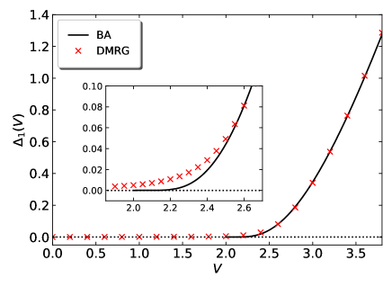
System sizes with an even particle number $N=L/2$ lead to an open-shell ground state at $V=0$, i.e., it is doubly degenerate. Therefore, the gap is exactly zero at $V=0$ in the absence of a symmetry-breaking term. In this way, systems with even $L/2$ minimize finite-size effects for small couplings.

In Fig. 5 we show the extrapolated single-particle gap as a function of $V$ from the polynomial fit together with the exact result from Bethe Ansatz, see eq. (34). The polynomial fit leads to a (very small) finite gap for all $V>0$, and the sharp transition in the exact solution at $V_{\rm c}=2$ is smeared out, as seen from the inset in Fig. 5, so that it is not possible to determine $V_{\rm c}$ with high accuracy from the extrapolated gaps. The standard polynomial extrapolation scheme does not permit to locate transitions at finite interaction strengths. This was shown recently for the Mott-Hubbard transition in the $1/r$-Hubbard model. Gebhard and Legeza (2021)

VI.3.2 Closed-shell systems with periodic boundary conditions

The Bethe Ansatz solution for the XXZ model permits to extract the finite-size corrections to the single-particle gap. Hamer (1985); Woynarovich and Eckle (1987) As seen in Sect. II.2, these Bethe Ansatz results can be applied to the model of spinless fermions only for odd particle numbers. Consequently, we have to study a closed-shell ground state at half band-filling with odd particle number $N=L/2$. Now that the excited state must also have an odd particle number, we must numerically study the ground state with two additional particles, $N=L/2+2$.

In the XXZ model, the two spin-1 excitations are very far from each other for large system sizes and we argue that the two-particle gap

$$\Delta_{2}^{\rm XXZ}(L,V)=2\left(E_{0}^{\rm XXZ}(S=2,L,V)-E_{0}(S=0,L,V)\right)$$ (149)

is twice as large as the single-particle gap in the thermodynamic limit,

$$\Delta_{1}^{\rm XXZ}(L,V)=\frac{\Delta_{2}^{\rm XXZ}(L,V)}{2}+{\cal O}(1/L^{\gamma})\;,$$ (150)

where corrections due the interaction of the excitations are of order $1/L^{\gamma}$ with $\gamma>1$. If this is the case, we can determine the $1/L$-correction to the single-particle gap from half of the two-particle gap. To this end, we extrapolate the DMRG data for spinless fermions

$$\frac{\Delta_{2}(L,V)}{2} = E_{0}(N=L/2+2,L,V)$$ (151)

$$\hphantom{\frac{1}{2}\Bigl{(}}-E_{0}(N=L/2,L,V)-2V$$

with a second-order polynomial in $1/L$,

$$\frac{\Delta_{2}(L,V)}{2}\approx\frac{\Delta_{2}(V)}{2}+\frac{s_{1}(V)}{L}+\frac{s_{2}(V)}{L^{2}}\;,$$ (152)

and compare $s_{1}(V)$ with the Bethe Ansatz result Hamer (1985); Woynarovich and Eckle (1987)

$$s_{1}^{\rm BA}(V) = 4\pi\left(1-\frac{\arccos(V/2)}{\pi}\right)$$

$$\times\left(2\sqrt{1-(V/2)^{2}}\left[\frac{\pi}{2\arccos(V/2)}\right]\right)\;.$$

Note that we work with the gap whereas the Bethe Ansatz formulae are derived for $\mu_{1}^{+,{\rm XXZ}}=\Delta_{1}/2$, and we adjusted the energy scale.

Figure 6: Slope $s_{1}(V)/(2\pi)$ in $1/L$ of half the two-particle gap $\Delta_{2}(V)/2$, see eqs. (151) and (152) from the extrapolation of the DMRG data (dots), in comparison with the Bethe Ansatz result (line) from eq. (VI.3.2). The horizontal line indicates the critical value $s_{1}(V_{\rm c})=(2\pi)^{2}$.

In Fig. 6 we compare the results for the slope $s_{1}(V)$ in eq. (152) from the polynomial fit of the DMRG data for $\Delta_{2}(L,V)/2$ and from the Bethe Ansatz expression (VI.3.2). The agreement is very good for small interactions but it deteriorates close to the transition. The criterion $s_{1}(V=V_{\rm c})=(2\pi)^{2}$, corresponding to $u(V_{\rm c})=\pi$ in the ground-state energy, leads to the estimate $V_{\rm c}^{\rm s}\approx 2.3$ from the extrapolated data for the slope $s_{1}(V)$. The result deviates from the exact result by some 15 percent. Therefore, the slope estimate is not very accurate, apart from the fact that additional information from the exact result is necessary to determine the value $s_{1}(V_{\rm c})$ at the transition.

VI.3.3 Open boundary conditions

For open boundary conditions, we must use the particle-hole symmetric form of the interaction,

$$\hat{V}_{\rm phs}=\sum_{l=1}^{L-1}(\hat{n}_{l}-1/2)(\hat{n}_{l+1}-1/2)\;.$$ (154)

If we used the interaction in eq. (4) adopted to a chain, excited states at the boundaries would interfere so that the bulk gap cannot be calculated from the ground state energies at half band-filling and with plus/minus one particle. This is most easily seen in the atomic limit, and will not be discussed any further.

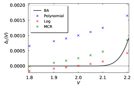
For the particle-hole symmetric Hamiltonian (2) on a chain, analytic finite-size corrections to the single-particle gap are not available. Therefore, we employ three different extrapolation schemes: polynomial, see eq. (148), logarithmic,

$$\Delta_{1}^{\rm ln}(L,V)=\Delta_{1}(V)+\frac{b_{1}}{L}\left(1+\frac{b_{2}}{\ln(L)}\right)\;,$$ (155)

and Mishra, Carrasquilla, and Rigol Mishra et al. (2011)

$$\Delta_{1}^{\rm MCR}(L,V)=\frac{\Delta_{1}(V)+c_{1}/L}{1+1/(2\ln(L)+c_{2})}\;,$$ (156)

where $b_{1,2}$ and $c_{1,2}$ are fit parameters.

In Fig. 7 we compare the resulting gaps in the critical region, $1.8\leq V\leq 2.2$ with the analytic result. Apparently, neither of the extrapolations can reliably determine the critical interaction because the extrapolated gaps always open smoothly. Without the exact result for comparison, we cannot decide which of the three schemes is superior to the two others. We examine extrapolation schemes for the single-particle gap in more detail in the supplemental material sup (see, also, reference [Carrasquilla et al., 2013] therein).

Figure 7: Exact single-particle gap $\Delta_{1}(V)$ in the thermodynamic limit in the range $1.8\leq V\leq 2.2$, in comparison with the result of three extrapolations of the DMRG data for open boundary conditions for $L=64,128,256,512$: polynomial (blue), eq. (148), logarithmic (red), eq. (155), and Mishra et al. (green), eq. (156).

VI.4 Order parameter

In Fig. 8 we show the CDW order parameter from DMRG as a function of the interaction for system sizes $L=128,256,512$. It is seen that the finite-size corrections are large for $V\lesssim 2.5$ but marginal for $V\gtrsim 3$. This indicates that very large system sizes are required to perform an accurate extrapolation to the thermodynamic limit in the vicinity of the critical interaction, $V_{\rm c}=2$.

As seen from the inset, Hartree-Fock theory predicts a continuous increase of the order parameter for $V>V_{\rm c}^{\rm HF}=0^{+}$. Second-order Hartree-Fock theory predicts a jump to a substantial CDW order at $V_{\rm c,2}^{(2)}\approx 1.5$. The curves start to coalesce around $V\gtrsim 4$ where the strong-coupling expansion becomes applicable. In general, second-order Hartree-Fock theory overestimates the CDW order parameter but less severely than the standard Hartree-Fock approximation.

Figure 8: Charge-density wave order parameter $n_{a}(L,V)$ as a function of the nearest-neighbor interaction $V$ from Bethe Ansatz (BA) and DMRG for $L=128,256,512$ sites. Inset: comparison of (second-order) Hartree-Fock and DMRG data for $L=512$ sites.

Finite-size effects are prominent in the DMRG data for the charge-density wave order parameter even for systems with $L=512$ sites. This does not come as a surprise because the CDW order parameter displays the same essential singularity as the single-particle gap, see eq. (42). As in the case of the single-particle gap, the second-order polynomial fit for the finite-size extrapolation,

$$n_{a}(L,V)=n_{a}(V)+\frac{d_{1}}{L}+\frac{d_{2}}{L^{2}}$$ (157)

with $n_{a}(V)$, $d_{1}$, and $d_{2}$ as fit parameters, leads to a smooth curve for $n_{a}(V)$, in contrast to the exact solution where the order sets in at $V_{\rm c}=2$. Therefore, the critical interaction strength cannot be deduced from the order parameter. We face the same difficulties for the single-particle gap that also displays an essential singularity at the transition.

VI.5 Correlation energy

The correlation energy can be calculated exactly from Bethe Ansatz results, see Sect. III.4. It goes to zero both for small and large interactions because the ground state is given by a single-particle product state in both cases, namely, a Slater determinant for free fermions at $V=0$ and a charge-density wave with a particle on every other lattice site for $V\to\infty$. Therefore, there is (at least) one extremum for finite $V$ at $V_{\rm corr}>0$.

Figure 9: Correlation energy at half band-filling as a function of the nearest-neighbor interaction $V$ from Bethe Ansatz (full line) and from DMRG for $L=512$ sites (crosses).

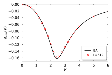
In Fig. 9 we show the correlation energy as a function of the interaction strength from Bethe Ansatz and from DMRG for $L=512$ sites. The overall agreement is very good. It is seen that the correlation energy is always negative. The single-particle contributions generically overestimate the interaction because they do not take the correlation hole into account that forms around the particles but only the exchange hole. The correlation energy has a (single) minimum but it is not located at the critical interaction but at $V_{\rm corr,min}\approx 2.4$, larger than $V_{\rm c}=2$ by some twenty percent.

Eq. (45) shows that various quantities contribute to the correlation energy. The ground-state energy and its derivative do not signal the metal-insulator transition whereas the order parameter $n_{a}(V)$ is finite for $V>V_{\rm c}$. The mixture of regular and critical quantities shifts the minimum of the correlation energy away from $V_{\rm c}$. This example shows that not every extremum in a physical quantity can be used to locate $V_{\rm c}$ with high precision.

VI.6 Momentum distribution

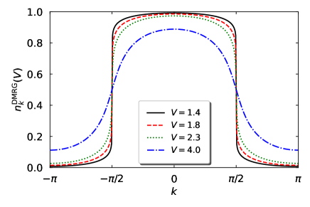
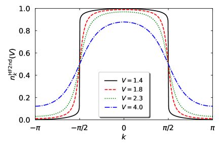
Next, we discuss the momentum distributions which have not been determined analytically from Bethe Ansatz for all $k$ and $V$ thus far. In Fig. 10 we show the momentum distribution $n_{k}=\langle\hat{a}_{k}^{+}\hat{a}_{k}^{\vphantom{+}}\rangle$. The points are dense enough to warrant continuous lines. It is known that the curves for $V>0$ are continuous in the thermodynamic limit with $n_{k=\pm\pi/2}=1/2$ due to particle-hole symmetry, see eq. (29) in Sect. III.5. The momentum distributions from DMRG in Fig. 10(a) and from second-order Hartree-Fock theory in Fig. 10(b) look very similar for $V=1.4,1.8,2.3,4$ but deviations close to the Fermi wave numbers $\pm\pi/2$ are clearly visible. Only for weak interactions, $V\lesssim 1$, and for large interactions, $V\gtrsim 6$, the curves for $n_{k}(V)$ in DMRG and (second-order) Hartree-Fock theory coalesce.

To identify the quantum phase transition from the DMRG data for the momentum distribution, we analyze $n_{k}(V)$ in the vicinity of the Fermi point $k_{\rm F}=\pi/2$. We rewrite eq. (50) as

$$\ln\left(1/2-n_{\pi/2+2\pi/L}(V)\right)=\ln[b(V)]+\alpha(V)\ln\left(2\pi/L\right)\;,$$ (158)

and extrapolate the DMRG data for the left-hand-side of eq. (158) in $\ln(L)$ to determine the fit parameters $\alpha(V)$ and $b(V)$. The result is shown if Fig. 11.

(a)
(b)

Figure 10: Momentum distribution $n_{k}$ for $V=1.4,1.8,2.3,4$ (a) from DMRG for $L=512$ lattice sites and (b) from second-order Hartree-Fock approximation.

The analytic Luttinger exponent $\alpha(V)$ from eqs. (46) and (47) is reproduced from DMRG for $V\leq 1.9$ but it is underestimated close to the transition so that the condition $\alpha^{\rm DMRG}(V_{\rm c}^{\alpha})=1/4$ leads to $V_{\rm c}^{\alpha}=2.2$. Likewise, the parameter $b(V)=1/2$ is observed with an accuracy of $10^{-3}$ deep in the Luttinger liquid but deviations of more than one percent occur for $V\gtrsim V_{\rm c}^{\beta}=1.8$. In this way, we locate the transition in the region $1.8=V_{\rm c}^{\beta}<V_{\rm c}<V_{\rm c}^{\alpha}=2.2$, within ten percent of the critical interaction.

Figure 11: Generalized Luttinger liquid exponent $\alpha(V)$ for spinless fermions at half band-filling as a function of the nearest-neighbor interaction $V$ extrapolated from DMRG and Bethe Ansatz (full line for $0\leq V\leq V_{\rm c}=2$). Inset: parameter $b(V)$.

VI.7 Quasi-particle distribution

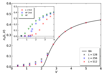
More intriguing than the momentum distribution is the quasi-particle distribution $n_{k,\beta}$. As we discussed in Sect. VI.1.2, $n_{k,\alpha/\beta}$ describes the occupation numbers for the natural orbitals that we identify with the lower $(k,\alpha)$ and upper $(k,\beta)$ Hartree-Fock bands.

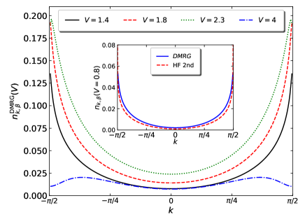
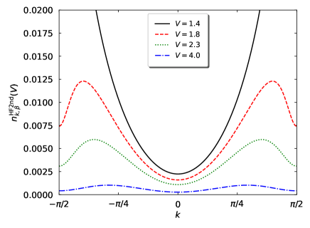
We show the quasi-particle distribution from DMRG in Fig. 12(a) and from second-order Hartree-Fock theory in Fig. 12(b). For $V<V_{\rm c}$ the DMRG data in Fig. 12(a) display a maximum at the band edges whereas in the insulating phase there are two maxima. Therefore, the onset of two maxima indicates the CDW transition, and a first estimate for the critical interaction strength can be deduced from the finite-size data, $V_{\rm c}^{\rm tm}\approx 2.15$.

The inset shows that the second-order results are in quantitative agreement with those from DMRG at weak coupling, $V=0.8$, which serves as a significant consistency check for both methods. As seen from a comparison of the main Figs. 12(a) and (b), the agreement between DMRG and second-order Hartree-Fock rapidly deteriorates for larger interactions, $V\gtrsim 1$. Even in the limit of strong interactions, the second-order Hartree-Fock approximation does not reproduce the DMRG data for the quasi-particle distribution. Although the curves look similar, they substantially differ quantitatively, by a factor of ten and more for $V\gtrsim 2$. In essence, Hartree-Fock theory severely underestimates the total density of quasi-particle excitations $n_{\beta}(V)$ defined in eq. (108).

To see this in more detail, we show the density of quasi-particle excitations $n_{\beta}(V)$ as a function of the interaction $V$ in Fig. 13. It is seen that the second-order Hartree-Fock theory is reliable only for $V\lesssim 1$. The quasi-particle density in Hartree-Fock theory displays a maximum just before and a jump discontinuity right at $V_{\rm c,2}^{(2)}\approx 1.5$, in agreement with the results in Sect. V.5. This observation indicates that $n_{\beta}(V)$ is a sensitive quantity to locate the CDW transition. Moreover, we see that $n_{\beta}^{(2)}(V)<0.011$ so that the condition for a dilute gas of quasi-particles, $n_{\beta}^{(2)}(V)\ll 1/2$ is always fulfilled. Therefore, second-order Hartree-Fock theory is applicable for all interaction strength and is ‘almost variational’, see Sect. V.2.

(a)
(b)

Figure 12: Quasi-particle distribution function $n_{k,\beta}$ for $V=1.4,1.8,2.3,4$ (a) from DMRG for $L=512$ lattice sites and (b) from second-order Hartree-Fock approximation. Note the factor ten difference in the values on the ordinate. Inset: DMRG and second-order Hartree-Fock for $V=0.8$.

The DMRG data for the quasi-particle density in Fig. 13 show that $n_{\beta}(V)<0.035$, i.e., it is never more than seven percent of its maximal value of one half. Therefore, the system can be viewed as a vacuum state with a dilute gas of quasi-particle excitations, even though second-order Hartree-Fock theory is not sufficient for its description beyond weak interactions.

Figure 13: Quasi-particle density $n_{\beta}(V)$ as a function of $V$ from DMRG for $L=128,256,512$, and from second-order Hartree-Fock theory.

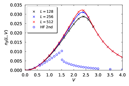
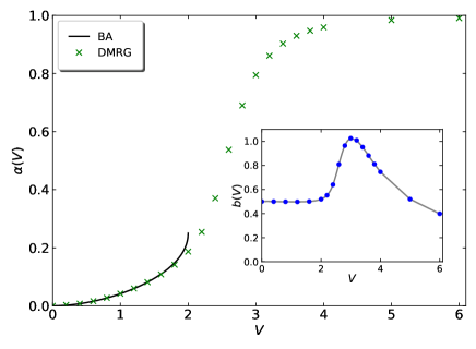
As seen in Fig. 13, the quasi-particle density is maximal close to the critical interaction strength, $V_{\rm c}=2$, so that we could use the maximum of the quasi-particle density to locate the exact CDW transition from a finite-size extrapolation. It turns out, however, that the finite-size scaling is logarithmic which limits the accuracy to several percent.

Figure 14: Values of the maxima in the quasi-particle density $n_{\beta}^{\rm max,k}(L,V)$ as a function of $V$ from DMRG for $L=32,64,128,256,512$. The continuous lines are a 6th-order polynomial fit for the region around the maximum.

To determine $V_{\rm c}$ more accurately, we recall that

$$n_{a}(V)=\frac{1}{L}\sum_{k\in{\rm RBZ}}\left(\langle\hat{a}_{k}^{+}\hat{a}_{k+\pi}^{\vphantom{+}}\rangle-\langle\hat{a}_{k+\pi}^{+}\hat{a}_{k}^{\vphantom{+}}\rangle\right)\;.$$ (159)

The exponential behavior of $n_{a}(V)$ close to the transition implies that most terms in the sum have a logarithmic dependence on system size. However, this does not exclude that some terms have an algebraic scaling in $1/L$ that is more suitable for finite-size extrapolations. In our analysis, we use the maximal value of the quasi-particle distribution

$$n_{\beta}^{\rm max,k}(L,V)=\mathop{\rm Max}_{k}n_{k,\beta}(L,V)$$ (160)

to locate such special $k$-values for a given interaction strength, see Fig. 12.

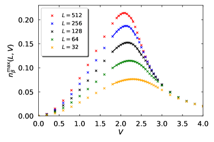
As seen in Fig. 14, the maximal value $n_{\beta}^{\rm max,k}(L,V)$ increases from zero for weak interactions up to a maximal value near the critical interaction strength and decreases down to zero for large interactions. We thus determine the maximum of $n_{\beta}^{\rm max,k}(L,V)$,

$$V_{\beta}^{\rm max}(L)=\mathop{\rm Max}_{V}n_{\beta}^{\rm max,k}(L,V)\;.$$ (161)

In Fig. 14 we show $n_{\beta}^{\rm max,k}(L,V)$ together with a 6th-order polynomial fit in the vicinity of $V=2$ to locate the positions $V_{\beta}^{\rm max}(L)$ for system sizes $L=32,64,128,256,512$. In this way, we locate $V_{\beta}^{\rm max}(L)$ with high accuracy.

Figure 15: Extrapolation of the maxima position in the quasi-particle density as a function of $1/L$ from DMRG for $L=64,128,256,512$. The continuous line is a fit to a second-order polynomial in $\sqrt{1/L}$.

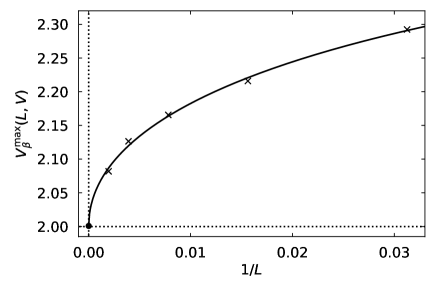
Next, we extrapolate the positions of the maxima to the thermodynamic limit. In Fig. 15 we show $V_{\beta}^{\rm max}(L)$ as a function of inverse system size together with a square-root fit,

$$V_{\beta}^{\rm max}(L)=V_{\rm c}^{\rm qp}+\frac{v_{1}}{\sqrt{L}}+\frac{v_{2}}{L}\;,$$ (162)

where $V_{\rm c}^{\rm qp}$, $v_{1}$, and $v_{2}$ are fit parameters. The square-root extrapolation is motivated by the fact that the Luttinger liquid is characterized by algebraic singularities. Indeed, the Luttinger parameter is $K(V_{\rm c})=1/2$ at the transition. The extrapolation results in $V_{\rm c}^{\rm qp}=2.0008\pm 0.019$, in agreement with the exact value for the critical interaction with at most one percent deviation. The extrapolation of the maxima position in the quasi-particle density provides a successful route to determine the critical interaction strength with high accuracy.

A more traditional route to determine the transition traces the breakdown of the Luttinger liquid, as already utilized for the finite-size corrections of the ground-state energy and of the gap. The Luttinger parameter $K(V)$ directly monitors the Luttinger liquid, as seen from the momentum distribution. Indeed, an accurate calculation of Luttinger exponent $K(V)$ from the density-density correlation function permits to locate the transition with an accuracy of three percent, as we shall show next.

VI.8 Density-density correlation function

Lastly, we address the density-density correlation function, eq. (51). We show its Fourier transform, eq. (53), from DMRG for $L=512$ sites and $V=1.8,2.3,4$ in Fig. 16. It is seen that the structure factor $\tilde{C}^{\rm NN}(q,V)$ shows the expected behavior, see Sect. III.6. It vanishes at $q=0$ with a finite slope for all $V$. It diverges for $|q|\to\pi$ in the Luttinger-liquid phase, and remains finite for all $q$ in the CDW phase.

Figure 16: Structure factor $\tilde{C}^{\rm NN}(q,V)$ from DMRG for $L=512$ sites for $V=1.4$ (black), $V=2.3$ (green), and $V=4$ (blue).
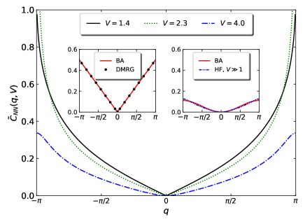
Left inset: Structure factor $\tilde{C}_{0}^{\rm NN}(q)$ from DMRG for $L=32$ sites and the analytic result (92) for $V=0$ (red line).
Right inset: Structure factor $\tilde{C}^{\rm NN}(q,V)$ from DMRG for $L=512$ sites for $V=6$ and the analytic result (96) for strong coupling (red line).

The insets of Fig. 16 show $\tilde{C}^{\rm NN}(q,V)$ for $V=0$ and for $V=6$, in comparison with the leading-order results for weak and strong coupling, see eqs. (92) and (96). At $V=0$, the agreement is excellent already for $L=32$ sites. For strong coupling, the agreement at $V=6$ is already very good but it is clearly seen that the corrections to order $1/V^{3}$ are important. This not only quantitatively applies at the Brillouin zone boundaries, $q=\pm\pi$, but also qualitatively close to $q=0$. Within Hartree-Fock theory, $\tilde{C}^{\rm NN}_{\rm BA}(q\to 0)\sim q^{2}$ whereas the exact density-density correlation function displays a kink at $q=0$, $\tilde{C}^{\rm NN}_{\rm HF}(q\to 0)\sim|q|$. This reflects the fact that the domain walls are mobile in the exact solution but rigid within the Hartree-Fock approximation. The freely mobile quasi-particles lead to a small-$q$ behavior resembling that of free fermions.

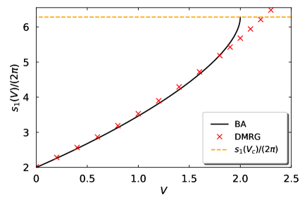
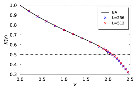
The main advantage of the density-density correlation function lies in the fact that it permits to determine the Luttinger parameter $K(V)$ with high accuracy. In Fig. 17 we show the exact result for $K(V)$ as a function of $V$ from Bethe Ansatz, eq. (47), in comparison with DMRG data for $L=256$ and $L=512$ sites. It is seen that the finite-size effects are of the same order of magnitude as the accuracy of the data. The agreement with the exact result is very good for $V\leq 1.95$, with deviations close to the transition. The field-theory criterion, $K(V_{\rm c})=1/2$, Giamarchi (2004) leads to $V_{\rm c}^{\rm LL}=2.06$. The analysis of $K(V)$ permits to locate the critical interaction with an accuracy of three percent.

Figure 17: Luttinger parameter $K(V)$ as a function of the interaction from the Fourier-transformed density-density correlation function at small $q$ from DMRG, eq. (54), for $L=256$ sites (blue crosses) and $L=512$ sites (red crosses), in comparison with the exact result (47) from Bethe Ansatz for $0\leq V\leq V_{\rm c}=2$ (black line).

VII Conclusions

A summary and a short outlook close our presentation on the charge-density wave transition for spinless fermions in one dimension.

VII.1 Summary

In this work, we study spinless fermions in one dimension with nearest-neighbor interaction $V$ and nearest-neighbor transfer matrix element $(-t)$ ($t\equiv 1$) at half band-filling. We use the Hartree-Fock approximation to first and second order in the interaction and the numerical density-matrix renormalization group (DMRG) for rings with up to 514 sites and compare the data with exact results from Bethe Ansatz in the thermodynamic limit. In particular, we investigate the ground-state energy per lattice site $e_{0}(V)$, the nearest-neighbor single-particle density matrix $B_{0}(V)$, the single-particle gap $\Delta_{1}(V)$, and the charge-density wave order parameter $n_{a}(V)$. For the ground-state energy and the gap, exact analytical formulae are available for the leading finite-size corrections in the metallic phase.

In addition, DMRG and second-order Hartree-Fock theory permit to calculate the single-particle density matrix and the density-density correlation function for all distances and thus provide the momentum distribution $n_{k}$, the quasi-particle distribution $n_{k,\beta}$, and the structure factor $\tilde{C}^{\rm NN}(q,V)$.

Hartree-Fock theory provides a good upper bound to the ground-state energy that is improved for all interaction strengths by including second-order corrections. Second-order Hartree-Fock theory is applicable for all interaction strengths because the density of quasi particles is very small so that second-order Hartree-Fock theory is almost variational.

In contrast to other exactly solvable one-dimensional models, spinless fermions display a charge-density-wave (CDW) transition at a finite value, $V_{\rm c}=2$. In standard Hartree-Fock theory, the CDW transition is predicted to set in at any finite interaction, reflecting the perfect nesting situation at half band-filling. Second-order Hartree-Fock theory predicts a discontinuous CDW transition at $V_{\rm c,2}^{\rm(2)}\approx 1.51$; the ordered phase around $V=0$ is reduced to the region $0<V<V_{\rm c,1}^{(2)}\approx 0.21$ and is characterized by a tiny order parameter. Therefore, second-order Hartree-Fock theory improves the description of spinless fermions considerably, both qualitatively and quantitatively.

Quantitatively reliable information about the CDW transition is obtained from DMRG on large systems. The exact ground-state energy density and nearest-neighbor single-particle density matrix do not display any singularities and are almost perfectly reproduced for all interaction strengths by DMRG for up to 514 sites. Likewise, the gap and the CDW order parameter are obtained with good accuracy from a finite-size extrapolation of the DMRG data, except for the critical region where the gap and the CDW order parameter display essential singularities. Therefore, different strategies have to be designed to locate the quantum phase transition accurately.

In this work, two strategies are designed that permit to determine the critical interaction strength. The traditional route focuses on the breakdown of the Luttinger liquid. Results from conformal field theory and the Bethe Ansatz for the finite-size corrections of the ground-state energy and the gap lead to useful but not very accurate estimates for $V_{\rm c}$. Moreover, these estimates require a lot of a-priori knowledge from the exact solution. Instead, the traditional derivation of the Luttinger parameter from the momentum distribution, $n_{k}(L,V)$, and, more accurately, from the structure factor at small momenta, $\tilde{C}^{\rm NN}(q\to 0,V)$, leads to $V_{\rm c}^{\rm LL}=2.06$, only three percent off the exact result. The second strategy to determine the CDW transition point with high accuracy utilizes the maxima of the quasi-particle distribution $n_{k,\beta}(L,V)$. For $L\to\infty$, $n_{\beta}^{\rm max,k}(V)$ peaks at $V_{\rm c}$. The finite-size extrapolation of DMRG data for up to $L=512$ sites leads to an agreement with one percent accuracy, $V_{\rm c}^{\rm qp}=2.0008\pm 0.019$.

The density of quasi-particles is small also for the exact solution, $n_{\beta}^{\rm max,k}(V)\leq 0.035\ll 0.5$. This implies that the system may be viewed as a vacuum state with a dilute gas of excitations. This observation ties in with the fact that dynamic correlation functions for the XXZ model can be expressed in terms as a series of $2n$-spinon excitations that is dominated by the first few terms.

VII.2 Outlook

The comparison with exact results from the Bethe Ansatz for spinless fermions in one dimension demonstrates that it is possible to locate Kosterlitz-Thouless transitions at finite interaction strengths from sophisticated extrapolations of DMRG data. Therefore, the strategies and extrapolation schemes proposed here can reliably be applied to non-integrable models in one dimension. The gapless phase of such models is described by a Luttinger liquid. As shown in this work, the quantum phase transition to a gapped phase can be detected by monitoring the Luttinger parameter obtained from the static density-density correlation function. Moreover, the quasi-particle densities depend on the ground-state phase, so that the occupation numbers of the natural orbitals provide a sensitive probe for locating Kosterlitz-Thouless-type phase transitions in generic one-dimensional many-particle models.

Our analysis also shows that second-order Hartree-Fock theory provides a reasonable description for all interaction strengths even in one spatial dimension. Therefore, we expect that it is useful to extend and apply the method to two and three dimensions where some peculiarities of one dimension are absent, e.g., freely moving domain walls in the strong-coupling limit. Work in this direction is in progress.

Supplemental material
Accurate localization of Kosterlitz-Thouless-type quantum phase transitions
for one-dimensional spinless fermions

The supplemental material consists of six parts. In supplement I, we examine various extrapolation schemes to extract the critical interaction strength from finite-size data for the charge-density wave order parameter and the single-particle gap. In supplements II, III, and IV, we provide the series expansion for the exact ground-state energy, order parameter, and single-particle gap, respectively. In supplement V, we calculate the matrix elements in second-order Hartree-Fock theory. In supplement VI, we derive observables in second-order Hartree-Fock approximation.

Supplement I Multi-parameter extrapolations

In the first section of the supplemental material, we scrutinize extrapolation schemes that aim to locate accurately the Kosterlitz-Thouless transition from finite-size data for the charge-density-wave (CDW) order parameter or the single-particle gap.

I.1 Extrapolation of the order parameter

In the main text, we use a polynomial extrapolation

$$n_{a}(L,V)=n_{a}(V)+\frac{d_{1}}{L}+\frac{d_{2}}{L^{2}}$$ (I-163)

with $n_{a}(V)$, $d_{1}$, and $d_{2}$ as fit parameters to estimate the charge-density-wave order parameter $n_{a}(V)$ in the thermodynamic limit. A much better fit for the CDW order parameter can be obtained from a logarithmic extrapolation of the DMRG data,

$$n_{a}^{\rm log}(L,V)=n_{a}^{\rm log}(V)+\frac{c}{(d+\ln(L))^{\gamma}}$$ (I-164)

with the four fit parameters $n_{a}^{\rm log}(V)$, $c$, $d$, and $\gamma$.

We extrapolate the DMRG data for the charge-density-wave order parameter $n_{a}(L,V)$ obtained for periodic boundary conditions and $L=64,128,256,512$, and plot $n_{a}^{\rm log}(V)$ in Fig. 18, together with the result from the second-order polynomial extrapolation $n_{a}(V)$ and the analytic result from Bethe Ansatz. As seen from the figure, the logarithmic fit procedure gives a much better agreement with the exact result even though the extrapolated order parameter is slightly negative below the transition and becomes positive around $V_{\rm c}$. This behavior is typical for transitions at finite interaction strengths. We may use the re-entrance criterion of a zero order parameter, $n_{a}(V_{\rm c}^{\rm re})=0$, to estimate the critical interaction strength. In this way we find $V_{\rm c}^{\rm re}=1.98$.

Figure 18: Charge-density wave order parameter $n_{a}(V)$ as a function of the nearest-neighbor interaction $V$ extrapolated from DMRG data (polynomial fit and logarithmic fit), in comparison with the exact Bethe-Ansatz solution (BA). Inset: exponent $\gamma(V)$: it is minimal at the exact critical interaction strength $V_{\rm c}=2$.

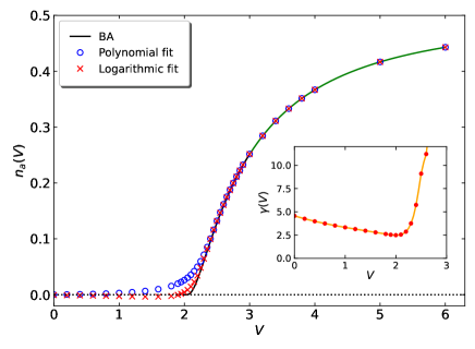
The critical interaction strength $V_{\rm c}$ can be determined with the same accuracy from the minimum of the exponent $\gamma(V)$. For our data set, the minimum of $\gamma(V)$ occurs at the exact value $V_{\rm c}=2$ so that the logarithmic extrapolation of the order parameter leads to $V_{\rm c}=2.00\pm 0.02$, with an accuracy of one percent.

However, this observation deserves some critical comments. First, the extrapolation includes four fit parameters which always carries the risk of over-fitting the data. Second, the functional form (I-164) is purely phenomenological. In fact, the same approximation leads to nonsensical results when applied to the single-particle gap. The logarithmic scheme (I-164) only coincidentally works for the CDW order parameter.

(a)	(b)
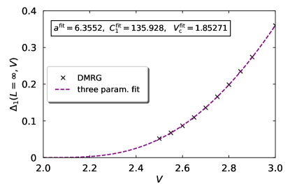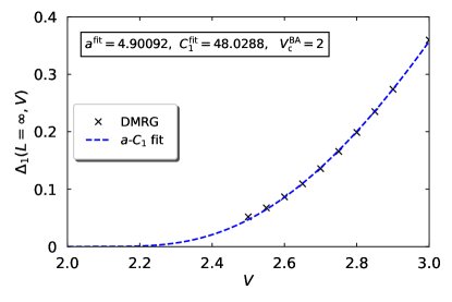(c)	(d)

Figure 19: DMRG single-particle gap $\Delta_{1}(V)$ as a function of the nearest-neighbor interaction $V$ extrapolated from DMRG data (polynomial fit), in comparison with (a) a three-parameter fit; (b) a two-parameter fit with fixed $V_{\rm c}=2$; (c) a two-parameter fit with fixed $C_{1}=16\pi$; (d) a two-parameter fit with fixed $a=\pi^{2}/2$.

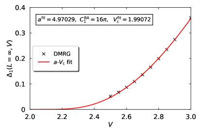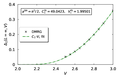I.2 Extrapolation of the single-particle gap

In the exact solution, the gap is exponentially small close to the transition,

$$\Delta_{1}(V\gtrsim 2)=16\pi\exp\left(-\frac{\pi^{2}/2}{\sqrt{V-2}}\right)$$ (I-165)

with an accuracy of better than seven percent for $V\lesssim 3$. Therefore, it is natural to fit the DMRG gaps, extracted from a second-order polynomial fit for the gap data for $L=64,128,256,512$, to the expression

$$\Delta_{1}(a,C_{1},V_{\rm c})=C_{1}\exp\left(-\frac{a}{\sqrt{V-V_{\rm c}}}\right)$$ (I-166)

with $C_{1}$, $a$, and $V_{\rm c}$ as fit parameters, where $a=\pi^{2}/2\approx 4.93$, $C_{1}=16\pi\approx 50.3$ and $V_{\rm c}=2$ are the exact values.

The application of the fit formula (I-166) generates several problems. First, for which parameters $V$ can the fit formula be applied? If $V$ is too large, we leave the asymptotic range; if $V$ is too small, the error in the extrapolated values from DMRG are too large. Below, we choose $2.5\leq V\leq 3$ to obtain meaningful results.

Second, an unbiased three-parameter fit leads to unsatisfactory results, as seen in Fig. 19(a). The DMRG gaps for $2.5\leq V\leq 3$ are faithfully reproduced but $C_{1}=136$, $a=6.36$, and $V_{\rm c}=1.85$ are far off the exact results. For a stable result, either $C_{1}$ or $a$ has to be close to its exact value. Using the guess $V_{\rm c}=2$, we obtain $C_{1}=48$ and $a=4.9$ as optimal values, quite close to the exact values, see Fig. 19(b). The two-parameter fit with the choice $C_{1}=16\pi$ leads to $a=4.97$ and $V_{\rm c}=1.99$, see Fig. 19(c), and for fixed $a=\pi^{2}/2$ we obtain $C_{1}=49$ and $V_{\rm c}=1.995$, and the values for all three parameters are very satisfactory. Note, however, that the least-square fit remains best for the three-parameter fit, case (a).

It is seen that the fitting of the gap requires a lot of a-priori information to obtain a good estimate for the critical interaction. Apparently, this is not a viable approach.

I.3 Scaling approach to the single-particle gap

To overcome the above limitations, Mishra, Carrasquilla, and Rigol designed a scaling approach Mishra et al. (2011) to extract $V_{\rm c}$ from the finite-size data so that an unspecific polynomial extrapolation is avoided and all raw data are included in the fit for $V_{\rm c}$.

The finite-size data are supposed to lie on a scaling curve,

$$L\Delta_{1}(L,V)\left(1+\frac{1}{2\ln(L)+C}\right)=F(L/\xi)\;,$$ (I-167)

where $\xi$ is the correlation length, and $F(x)$ is the unknown scaling function. Here, $C$ is a number that is independent of $L$ and $V$ in the critical regime. The functional form on the left-hand-side of eq. (I-167) is motivated from the scaling behavior of the conductivity in two-dimensional systems with a Kosterlitz/Thouless transition at finite temperatures. Mishra et al. (2011)

Close to the transition, the correlation length on the insulating side should diverge proportional to the inverse gap,

$$\ln\xi=\frac{a}{\sqrt{V-V_{\rm c}}}\sim-\ln(\Delta)\;.$$ (I-168)

Therefore, it is advisable to employ not $L/\xi$ but $x_{L}=\ln(L/\xi)=\ln(L)-a/\sqrt{V-V_{\rm c}}$ as variable in the scaling function, i.e., $F(L/\xi)\equiv f(x_{L})$ in eq. (I-167). To make progress, it must be assumed that in the region of accessible values for $L$ and $V$, the scaling function $f(x_{L})$ can reliably be represented by a polynomial of order $R$

$$f(x_{L})\approx\sum_{r=0}^{R}\alpha_{r}(x_{L})^{r}\;,$$ (I-169)

where the coefficients $\alpha_{r}$ remain to be determined. Here, $R$ should be chosen such that the absolute value of the real coefficient $\alpha_{r}\sim 10^{-r}$ is small. Below, we shall use $R=5$.

The remaining task is to find the optimal fit of the numerical data to the scaling form, i.e., we minimize the penalty function Carrasquilla et al. (2013)

$$S(a,C,v_{\rm c},\left\{\alpha_{r}\right\}) = \sum_{i,j}\biggl{[}L_{i}\Delta_{1}(L_{i},V_{j})\Bigl{[}1+\frac{1}{2\ln(L_{i})+C}\Bigr{]}$$

$$-\sum_{r=0}^{R}\alpha_{r}\Bigl{(}\ln(L_{i})-\frac{a}{\sqrt{V_{j}-V_{\rm c}}}\Bigr{)}^{r}\biggr{]}^{2}$$

with respect to the Taylor coefficients $\alpha_{r}$ and the parameters $a,C,V_{\rm c}$. Here, we include the gap data $\Delta_{1}(L_{i},V_{j})$ for the system sizes $L_{i}\in\{128,256,512\}$ and interaction strengths $V_{j}\in\{2.15,2.2,2.25,2.3,2.35,2.4,2.45,2.5\}$. As seen from eq. (LABEL:suppeq:penaltyfunction), we cannot select values $V_{i}$ that are too close to the transition because, due to the factor $1/\sqrt{V_{i}-V_{\rm c}}$, the range of values for $x_{L}$ becomes too large for the series expansion.

The minimization task posed by eq. (LABEL:suppeq:penaltyfunction) is non-trivial. It is done in two steps. First, for fixed $(C,a,V_{\rm c})$, the minimization implies a least-square fit of the data to the scaling function. This quadratic problem is readily solved by using FindMinimum of Mathematica.Wolfram Research, Inc. (2021).

In the second step, $(C,a,V_{\rm c})$ are optimized. This can either be done by using a dense grid of values for $(C,a,V_{\rm c})$ around some educated guess $(C,a,V_{\rm c})_{0}$, and picking the lowest values for the penalty function to determine the optimal set of parameters. Carrasquilla et al. (2013) Alternatively, we apply a sequence of optimizations by first optimizing $C$ for given $(a,V_{\rm c})$, then we optimize $a$ while re-optimizing $C$ whenever $a$ changes. As soon as $(C,a)$ are optimal for the given $V_{\rm c}$, we optimize $V_{c}$ for this set. The procedure is repeated with the optimization of $(C,a)$ for the new value for $V_{\rm c}$ and terminates when the penalty function changes by less than $10^{-5}$. The final result does not depend on the sequence of optimizations. The results agree with those obtained from the dense-grid method.

The best result is $S=0.226466$ for the parameter set $C=-15.758$, $a=5.12388$, and $V_{\rm c}=2.01105$. The data and the scaling curve are shown in Fig. 20. Apparently, a nice agreement with the exact data, $a=\pi^{2}/2\approx 4.93$, and $V_{\rm c}=2$ is obtained. The agreement is slightly worse, $S=0.413908$ for the parameter set $C=-15.682$, $a=5.1743$, and $V_{\rm c}=2.02$ when the data for $L=64$ are included. This signals that the inclusion of larger system sizes systematically lead to better results for the critical interaction strength.

Figure 20: Finite-size data for the single-particle gap, plotted as $y_{L}(L_{i},V_{j})=L_{i}\Delta_{1}(L_{i},V_{j})\left[1+1/(2\ln(L_{i})+C)\right]$ versus the scaling parameter $x_{L}=\ln(L_{i})-a/\sqrt{V_{j}-V_{\rm c}}$, together with the corresponding scaling function $f(x_{L})$. For the chosen parameter sets, see text.

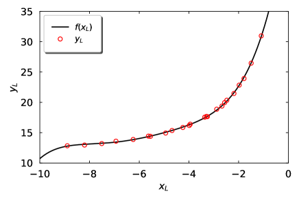
The degree $R$ of the polynomial is a more sensitive parameter. When we choose $R=4$ instead of $R=5$, we obtain $S=0.623039$ for the parameter set $C=-15.9479$, $a=6.332$, and $V_{\rm c}=1.93$. At the same time, $R=6$ leads to $S=0.0779472$ for the parameter set $C=-15.588$, $a=4.5168$, and $V_{\rm c}=2.06$. Apparently, the least-square fit needs to be stabilized by providing more data points, i.e., DMRG data for more system sizes and interaction strengths ($L_{i},V_{j})$.

More problematic than the selection of $R$ is the sign of the constant $C$. Since it is negative, there is a system size $L_{C}=\exp(-C/2)\approx 2600$ where the assumption of a logarithmic correction in eq. (I-167) becomes meaningless. Apparently, the logarithmic term is needed to stabilize the extrapolation scheme for $L\ll L_{C}$. Indeed, without the logarithmic term, the critical interaction would be far off the exact value, $V_{\rm c}=1.6$. We also found that the factor $L$ in front of $\Delta_{1}(L,V)$ in eq. (I-167) is essential to obtain meaningful values for $V_{\rm c}$. Moreover, the dependence of the correlation length on $1/\sqrt{V-V_{\rm c}}$ in eq. (I-168) is taken for granted. We come to the conclusions that the scaling approach cannot be used as a black box tool to derive $V_{\rm c}$ with good accuracy.

Supplement II Series expansions for the exact ground-state energy

In this appendix, we give the Taylor series expansions for weak and strong interactions, and asymptotic series expansions around the critical interaction strength for the ground-state energy at half band-filling. To this end, we use the original expressions by Yang and Yang. A more sophisticated approach employs special functions. Göhmann (2022)

II.1 Approximation for weak interactions

For weak interactions, we use the representation of $g(\mu)$ given by Yang and Yang, Yang and Yang (1966a, b)

$$g(\mu) = \frac{\cos(\mu)}{4}-\frac{2\sin(\mu)}{\mu}Y(\mu)\;,$$

$$Y(\mu) = \ln(2)-2\int_{0}^{\infty}{\rm d}y\frac{\tanh(y)}{\exp(2\pi y/\mu)-1}\;.$$ (II-171)

We introduce $\gamma=\pi/2-\mu$ so that

$$\sin(\gamma)=\frac{V}{2}\;,$$ (II-172)

and write

$$Y(\gamma) = \ln(2)-\left(\frac{1}{2}-\frac{\gamma}{\pi}\right)Z(\gamma)\;,$$

$$Z(\gamma) = \int_{0}^{\infty}{\rm d}u\frac{\tanh[u/4-\gamma u/(2\pi)]}{e^{u}-1}\;.$$ (II-173)

Using Mathematica, Wolfram Research, Inc. (2021) the series expansion for $Z(\gamma)$ around $\gamma=0$ reads

$$Z(\gamma) = 2\ln(2)-1-\left(\frac{1-4\ln(2)}{\pi}+\frac{\pi}{4}\right)\gamma$$ (II-174)

$$-\frac{4(3+\pi^{2}-18\ln(2))}{9\pi^{2}}\gamma^{2}$$

$$\frac{-48-32\pi^{2}+\pi^{4}+384\ln(2)}{24\pi^{3}}\gamma^{3}$$

$$+\frac{16(-135-150\pi^{2}+7\pi^{4}+1350\ln(2))}{675\pi^{4}}\gamma^{4}$$

$$+{\cal O}\left(\gamma^{5}\right)\;.$$

Collecting all terms and using eq. (II-172), Mathematica Wolfram Research, Inc. (2021) gives

$$e_{0}(V,N=L/2) = -\frac{2}{\pi}+\left(\frac{1}{4}-\frac{1}{\pi^{2}}\right)V$$ (II-175)

$$+\left(-\frac{2}{3\pi^{3}}+\frac{1}{36\pi}\right)V^{2}$$

$$+\left(\frac{1}{32}-\frac{1}{2\pi^{4}}-\frac{1}{4\pi^{2}}\right)V^{3}$$

$$+\left(-\frac{2}{5\pi^{5}}-\frac{5}{12\pi^{3}}+\frac{73}{1600\pi}\right)V^{4}$$

$$+{\cal O}\left(V^{5}\right)\;.$$

The accuracy of the Taylor series is better than one percent for $0\leq V\leq 2$.

II.2 Approximation for large interactions

For $V>2$ we write the ground-state energy for spinless fermions at half band-filling in the form

$$e_{0}(V)=e^{-\lambda}-4\sinh(\lambda)\sum_{n=1}^{\infty}\frac{1}{1+\exp(2\lambda n)}$$ (II-176)

with $\lambda=\lambda(V)={\rm arcosh}(V/2)$.

For large $V$, only a limited number of terms in the sum needs to be included. Using Mathematica Wolfram Research, Inc. (2021) then gives the large-$V$ asymptotics

$$e_{0}(V>2) = -V^{-1}+V^{-3}-V^{-7}-2V^{-9}$$ (II-177)

$$-2V^{-11}+2V^{-13}+17V^{-15}$$

$$+56V^{-17}+134V^{-19}$$

$$+{\cal O}\left(V^{-21}\right)\;.$$

The accuracy of the approximation is $10^{-4}$ for $V\geq 2$.

II.3 Approximation close to the transition

Around the critical interaction $V_{\rm c}=2$, the ground-state energy can be expressed in terms of an asymptotic series in the metallic and in the insulating region, respectively.

II.3.1 Metallic region

We start from eq. (16) in the main text. Yang and Yang Yang and Yang (1966a, b) provide an asymptotic series around $\mu=0$. We can either follow Yang and Yang who give an analytic expression for the series coefficients, or we obtain the lowest-order coefficients from a Taylor series of the integrand in $g(\mu)$. The resulting integrals can be done with Mathematica, Wolfram Research, Inc. (2021) apart from the leading order,

$$\int_{-\infty}^{\infty}{\rm d}x\frac{1}{(1+4x^{2})\cosh(\pi x)}=\ln(2)\;,$$ (II-178)

that requires a contour integral for its evaluation. Yang and Yang (1966a, b) We find

$$g(\mu) = \frac{1}{2}-2\ln(2)+\frac{1}{12}\left(4\ln(2)-1\right)\mu^{2}$$ (II-179)

$$-\frac{1}{240}\left(3+4\ln(2)\right)\mu^{4}$$

$$+\frac{1}{10080}\left(27+4\ln(2)\right)\mu^{6}+{\cal O}\left(\mu^{8}\right)\;.$$

Thus, for $V\lesssim 2$, we obtain for the ground-state energy of spinless fermions up to second order

$$e_{0}(V) = 1-2\ln(2)$$ (II-180)

$$+\frac{1}{3}\left(1-\ln(2)\right)\left(V-2\right)$$

$$+\frac{1}{360}\left(-7+4\ln(2)\right)\left(V-2\right)^{2}$$

$$+{\cal O}\left((V-2)^{3}\right)\;.$$

The approximation is better than two per mille for $0\leq V\leq 2$. The next order reduces the accuracy down to five per mille for $0\leq V\leq 2$. Recall that the series is only asymptotic.

For comparison, we give the asymptotic result for the ground-state energy up to fifth order,

$$e_{0}(V) = 1-2\ln(2)$$ (II-181)

$$+\frac{1-\ln(2)}{3}\left(V-2\right)$$

$$+\frac{4\ln(2)-7}{360}\left(V-2\right)^{2}$$

$$\frac{1-4\ln(2)}{3024}\left(V-2\right)^{3}$$

$$+\frac{184\ln(2)-487}{907200}\left(V-2\right)^{4}$$

$$-\frac{2104\ln(2)+14153}{59875200}\left(V-2\right)^{5}$$

$$+{\cal O}\left((V-2)^{6}\right)\;.$$

We shall show below that it agrees with the corresponding expression in the insulating region.

II.3.2 Insulating region

We start from eq. (16) of the main text. First, we write

$$S(\lambda) \equiv \sum_{n=1}^{\infty}\frac{1}{1+\exp(2\lambda n)}$$ (II-182)

$$= \sum_{n=1}^{\infty}\sum_{r=0}^{\infty}(-1)^{r}e^{-2\lambda(r+1)n}$$

$$= -\sum_{r,n=1}^{\infty}(-1)^{r}e^{-2\lambda rn}$$

$$= \sum_{r=1}^{\infty}(-1)^{r}\frac{1}{1-\exp(2\lambda r)}\;.$$

The rearrangement of the sum shows directly that, in the limit $\lambda\to 0$,

$$S(\lambda\to 0)=-\frac{1}{2\lambda}\sum_{r=1}^{\infty}(-1)^{r}\frac{1}{r}=\frac{\ln(2)}{2\lambda}\;.$$ (II-183)

Therefore,

$$h(0)=\frac{1}{2}-4\lim_{\lambda\to 0}\lambda S(\lambda)=\frac{1}{2}-2\ln(2)$$ (II-184)

in eq. (18) of the main text, as it must be because the ground-state energy is continuous at $V=2$.

To make further progress, we define

$$f_{1}(\lambda,m) = \frac{1}{\exp[2\lambda(2m)]-1}-\frac{1}{2\lambda(2m)}\;,$$

$$f_{2}(\lambda,m) = \frac{1}{\exp[2\lambda(2m-1)]-1}-\frac{1}{2\lambda(2m-1)}\;,$$

so that

$$S(\lambda) = \sum_{m=1}^{\infty}\left(f_{2}(\lambda,m)-f_{1}(\lambda,m)\right)$$ (II-186)

$$+\sum_{m=1}^{\infty}\left(\frac{1}{2\lambda(2m-1)}-\frac{1}{2\lambda(2m)}\right)$$

$$= \sum_{m=1}^{\infty}\left(f_{2}(\lambda,m)-f_{1}(\lambda,m)\right)+\frac{\ln(2)}{2\lambda}\;.$$

For the sum we invoke the Euler-Maclaurin sum formula to construct an asymptotic series expansion for small $\lambda$,

$$\sum_{m=1}^{M}F(m) \sim \int_{1}^{\infty}{\rm d}xF(x)+\frac{1}{2}\left(F(M)+F(1)\right)$$

$$+\sum_{k}\frac{B_{2k}}{(2k)!}\left(F^{(2k-1)}(M)-F^{(2k-1)}(1)\right)\;.$$

We must calculate the following three terms. The integral terms reads

$$T_{1}(\lambda) = \int_{1}^{\infty}{\rm d}xf_{2}(\lambda,x)-\int_{1}^{\infty}{\rm d}xf_{1}(\lambda,x)$$ (II-188)

$$= \int_{1/2}^{\infty}{\rm d}xf_{1}(\lambda,x)-\int_{1}^{\infty}{\rm d}xf_{1}(\lambda,x)$$

$$= \frac{1}{4\lambda}\int_{2\lambda}^{4\lambda}{\rm d}u\left(\frac{1}{e^{u}-1}-\frac{1}{u}\right)$$

$$= \frac{\ln[\cosh(\lambda)]}{4\lambda}-\frac{1}{4}\;.$$

The second term is

$$T_{2}(\lambda)=\frac{1}{2}\left(f_{2}(\lambda,1)-f_{1}(\lambda,1)\right)=\frac{1}{4\sinh(2\lambda)}-\frac{1}{8\lambda}\;.$$ (II-189)

The third term involves the derivatives of $f_{2}(\lambda,x)-f_{1}(\lambda,x)$ at $x=1$ that we expand in a Taylor series around $\lambda=0$. We note that

$$\left.\left(\frac{\partial}{\partial x}\right)^{2k-1}\left(f_{2}(\lambda,x)-f_{1}(\lambda,x)\right)\right|_{x=1}\sim\lambda^{2k+1}\;,$$ (II-190)

so that in the remaining series over the derivatives we have

$$T_{3}(\lambda)+T_{3}^{(K)}(\lambda)={\cal O}\left(\lambda^{2K+3}\right)$$ (II-191)

with

$$T_{3}^{(K)}(\lambda)=\sum_{k=1}^{K}\frac{B_{2k}}{(2k)!}\left(f_{2}^{(2k-1)}(\lambda,1)-f_{1}^{(2k-1)}(\lambda,1)\right)\;.$$ (II-192)

In fact, Mathematica gives

$$T_{3}^{(4)}(\lambda)=-\frac{\lambda^{3}}{60}+\frac{\lambda^{5}}{90}-\frac{\lambda^{7}}{6300}+\frac{101\lambda^{9}}{44550}$$ (II-193)

for $\lambda\ll 1$. The series expansion for $S(\lambda)$ thus becomes

$$S(\lambda) = \frac{\ln(2)}{2\lambda}+T_{1}(\lambda)+T_{2}(\lambda)+T_{3}(\lambda)$$ (II-194)

$$\sim \frac{\ln(2)}{2\lambda}-\frac{1}{4}+\frac{\lambda}{24}+\frac{\lambda^{3}}{720}+\frac{\lambda^{5}}{3780}+\frac{17\lambda^{7}}{151200}$$

$$+\frac{31\lambda^{9}}{374220}+{\cal O}\left(\lambda^{11}\right)\;.$$

The approximation is better than $10^{-4}$ for $0\leq\lambda\leq 0.9$.

Thus, the expansion of the ground-state energy close to the transition in the insulating phase becomes for $V\gtrsim 2$

$$e_{0}(V) = 1-2\ln(2)$$ (II-195)

$$+\frac{1-\ln(2)}{3}\left(V-2\right)$$

$$+\frac{4\ln(2)-7}{360}\left(V-2\right)^{2}$$

$$+\frac{1-4\ln(2)}{3024}\left(V-2\right)^{3}$$

$$+\frac{184\ln(2)-487}{907200}\left(V-2\right)^{4}$$

$$-\frac{2104\ln(2)+14153}{59875200}\left(V-2\right)^{5}$$

$$+{\cal O}\left((V-2)^{6}\right)\;.$$

The approximation is better than $10^{-3}$ only for $2\leq V\leq 3$, i.e., the approximation is not particularly useful.

Note that the asymptotic series in the insulating regime, eq. (II-195) for $V\geq 2$, agrees with the asymptotic expansion in the metallic regime, eq. (II-181) for $0<V\leq 2$. This does not come as a surprise because the ground-state energy is continuously differentiable at $V=2$ to all orders.

Supplement III Series expansion for the exact single-particle gap

In this appendix we provide formulae for the single-particle gap in the strong-coupling limit and close to the transition where it opens exponentially. A more sophisticated approach employs Jacobi $\theta$-functions. Göhmann (2022)

III.1 Strong coupling

We rewrite eq. (32) of the main text as

$$\frac{V}{2}=\frac{1}{2}\left(e^{r(m)}+e^{-r(m)}\right)$$ (III-196)

with

$$r(m)=\frac{\pi K(1-m)}{K(m)}\;.$$ (III-197)

For large $V$, we have $m\to 0$ so that the Taylor series gives

$$\frac{V}{2} = -4+\frac{8}{m}-\frac{19m}{32}-\frac{19m^{2}}{64}-\frac{767m^{3}}{4096}-\frac{1085m^{4}}{8192}$$ (III-198)

$$-\frac{105227m^{5}}{1048576}-\frac{166967m^{6}}{2097152}-\frac{35047971m^{7}}{536870912}$$

$$+{\cal O}\left(m^{8}\right)\;.$$

We set $x=mV$ and use the expansion

$$x(V)=\sum_{r=0}^{7}a_{r}\frac{1}{V^{r}}$$ (III-199)

to solve eq. (III-198) iteratively. The result is

$$m(V) = \frac{16}{V}-\frac{128}{V^{2}}+\frac{720}{V^{3}}-\frac{3328}{V^{4}}+\frac{13632}{V^{5}}-\frac{51328}{V^{6}}$$ (III-200)

$$+\frac{181488}{V^{7}}-\frac{611072}{V^{8}}+\frac{1977904}{V^{9}}$$

$$+{\cal O}\left(V^{-10}\right)\;.$$

We insert this solution in eq. (34) of the main text and let Mathematica Wolfram Research, Inc. (2021) do the expansion,

$$\Delta_{1}(V\gg 2) = 2V-8+\frac{4}{V}+\frac{8}{V^{2}}+\frac{4}{V^{3}}-\frac{8}{V^{6}}-\frac{12}{V^{7}}$$ (III-201)

$$+{\cal O}\left(V^{-8}\right)\;.$$

The accuracy of the approximation is better than $4\cdot 10^{-4}$ for $V\geq 4$. The accuracy rapidly deteriorates below $V=3$ where the deviation is about two percent.

III.2 Transition region

Close to the transition, we have $m\to 1$ and thus we must solve

$$\gamma\approx-\frac{\pi^{2}}{\ln\left((1-m)/16\right)}$$ (III-202)

in eq. (32) of the main text. Therefore, $m$ is exponentially close to unity for $V\to 2^{+}$,

$$m(V)\approx 1-16\exp\left(-\frac{\pi^{2}}{\gamma}\right)\approx 1-16\exp\left(-\frac{\pi^{2}}{\sqrt{V-2}}\right)\;.$$ (III-203)

Using the series expansion of the elliptic integral we finally find for the single-particle gap

$$\Delta_{1}(V\to 2^{+})\to 16\pi\exp\left(-\frac{\pi^{2}}{2\sqrt{V-2}}\right)\;.$$ (III-204)

Eq. (III-204) shows that the gap becomes exponential small close to the critical interaction.

The accuracy of the approximate result (III-204) is not impressive because it is only better than seven percent for $2\leq V\leq 3$. A better approximation is given by

$$m(V) \approx 1-16\exp\left(-\frac{\pi^{2}}{{\rm arcosh}(V/2)}\right)$$

$$+128\exp\left(-\frac{2\pi^{2}}{{\rm arcosh}(V/2)}\right)\;,$$

$$\Delta_{1}(V\gtrsim 2) \approx \frac{8}{\pi}\sqrt{\left[\left(V/2\right)^{2}-1\right]\left[1-m(V)\right]}$$

$$\times\biggl{[}-\frac{1}{2}\ln\left[\frac{1-m(V)}{16}\right]$$

$$\hphantom{\times\biggl{[}}+\frac{m(V)-1}{8}\left(2+\ln\left[\frac{1-m(V)}{16}\right]\right)\biggr{]}\;.$$

The accuracy of the approximation (LABEL:eq:usethisforsmallV) is better than $10^{-5}$ for $2\leq V\leq 4$. It remains better than one per mille for $2\leq V\leq 6$.

Supplement IV Series expansion for the exact order parameter

In this appendix we provide formulae for the order parameter gap in the strong-coupling limit, and close to the transition where it opens exponentially. A more sophisticated approach employs Jacobi $\theta$-functions and their derivatives. Göhmann (2022)

IV.1 Strong coupling

For strong coupling we have $q=2|\Delta|=V$ to leading order, and only the first term in the product (38) of the main text needs to be included,

$$n_{a}(V\gg 1) \approx \frac{1}{2}\left(1-\frac{2}{q^{2}}\right)^{2}$$ (IV-206)

$$\approx \frac{1}{2}\left(1-\frac{4}{V^{2}}\right)=\frac{1}{2}-2\left(\frac{1}{V}\right)^{2}\;.$$

Using Mathematica Wolfram Research, Inc. (2021) we can easily obtain the series up to order $V^{-12}$,

$$n_{a}(V\gg 1) \approx \frac{1}{2}-2\left(\frac{1}{V}\right)^{2}-2\left(\frac{1}{V}\right)^{4}-2\left(\frac{1}{V}\right)^{6}$$ (IV-207)

$$+2\left(\frac{1}{V}\right)^{8}+24\left(\frac{1}{V}\right)^{10}+114\left(\frac{1}{V}\right)^{12}$$

$$+{\cal O}\left(V^{-14}\right)\;.$$

The series expansion agrees with the exact expression down to $V=3$ with an accuracy of better than one half per mille.

IV.2 Transition region

A rigorous expansion of the product formula in eq. (38) of the main text is not trivial. We write

$$s_{0}(q) = \left(\frac{f_{1}(q)}{f_{2}(q)}\right)^{2}\;,$$

$$f_{1}(q) = \prod_{m=1}^{\infty}\left(1-q^{-2m}\right)\;,$$

$$f_{2}(q) = \prod_{m=1}^{\infty}\left(1+q^{-2m}\right)\;,$$ (IV-208)

and treat the two functions $f_{1,2}(q)$ separately.

IV.2.1 First function

By definition, $f_{1}(q)$ can be written as

$$f_{1}(q)=\left(\frac{1}{q^{2}};\frac{1}{q^{2}}\right)_{\infty}\;,$$ (IV-209)

where $(a;Q)_{\infty}$ is the Q-Pochhammer function. For $q\to 1^{+}$, Banerjee and Wilkerson provide the result Banerjee and Wilkerson (2017)

$$f_{1}(q)=\sqrt{\frac{\pi}{\ln(q)}}\exp\left(-\frac{\pi^{2}}{12\ln(q)}\right)q^{1/12}\;,$$ (IV-210)

which agrees with the exact numerical value with an accuracy of $10^{-4}$ up to $q=8$.

IV.2.2 Second function

$f_{2}(q)$ can also be expressed in terms of the Q-Pochhammer function,

$$f_{2}(q)=\frac{1}{2}\left(-1;\frac{1}{q^{2}}\right)_{\infty}\;.$$ (IV-211)

Garoufalidis and Zagier provide an approximation for $(wQ^{x};Q)_{\infty}$ for general $Q\to 1^{-}$.Garoufalidis and Zagier (2021) It is permitted to use their formula for $w=-1$ and $x=0$ so that we find

$$\ln\left[2f_{2}(q)\right] = B_{0}(0){\rm li}_{2}(-1)\frac{1}{\ln(1/q^{2})}+B_{1}(0){\rm li}_{1}(-1)$$

$$+\frac{1}{2}B_{2}(0){\rm li}_{0}(-1)\ln(1/q^{2})+\ldots$$

$$\approx -\frac{\pi^{2}}{12\ln(1/q^{2})}+\frac{\ln(2)}{2}+\frac{1}{12}\Bigl{(}-\frac{1}{2}\Bigr{)}\ln\biggl{[}\frac{1}{q^{2}}\biggr{]},$$

where $B_{k}(x)$ is the $k$th Bernoulli polynomial and ${\rm li}_{k}(z)$ is the poly-logarithm of order $k$. Therefore, the approximation for $q\to 1^{+}$ becomes

$$f_{2}(q) \approx \frac{1}{2}\exp\left(\frac{\pi^{2}}{24\ln(q)}+\frac{\ln(2)}{2}+\frac{\ln(q)}{12}\right)$$ (IV-213)

$$= \frac{\sqrt{2}}{2}q^{1/12}\exp\left(\frac{\pi^{2}}{24\ln(q)}\right)\;.$$

The approximation reproduces the exact result with an accuracy of $10^{-4}$ up to $q=4$.

IV.2.3 Final result close to the transition

Using eqs. (IV-210) and (IV-213) we find

$$s_{0}(q)\approx\frac{2\pi}{\ln(q)}\exp\left(-\frac{\pi^{2}}{4\ln(q)}\right)\;.$$ (IV-214)

The approximation agrees with the exact result with an accuracy of better than $10^{-3}$ up to $q=3$.

With

$$q(V)=\frac{V}{2}+\sqrt{\left(\frac{V}{2}\right)^{2}-1}$$ (IV-215)

we thus have for the order parameter

$$n_{a}(V)\approx\frac{\pi}{\ln(q(V))}\exp\left(-\frac{\pi^{2}}{4\ln(q(V))}\right)$$ (IV-216)

with an accuracy of better than $10^{-4}$ for $2\leq V\leq 3$.

IV.2.4 Alternative derivation

A fast but less rigorous way to derive eq. (IV-214) starts from

$$\ln\left(\frac{f_{1}(q)}{f_{2}(q)}\right)=\sum_{m=1}^{\infty}\ln\left[\tanh(\alpha m)\right]\;,$$ (IV-217)

where we set $\alpha=\ln(q)$. With the help of the Euler-Maclaurin sum formula we find up to order $\alpha$

$$\ln\left(\frac{f_{1}(q)}{f_{2}(q)}\right) = \int_{1}^{\infty}{\rm d}x\ln\left[\tanh(\alpha x)\right]+\frac{1}{2}\ln\left[\tanh(\alpha)\right]$$ (IV-218)

$$-\sum_{k=1}^{p}\frac{B_{2k}}{(2k)!}g^{(2k-1)}(1)+R_{p,k}$$

$$+{\cal O}\left(\alpha\right)$$

with $g(x)=\ln\tanh(\alpha x)$. For small $\alpha$ we see that $g(x)\approx\ln(\alpha)+\ln(x)$ so that the terms in the second line reduce to the same expression as obtained for the Stirling formula. Therefore,

$$\ln\left(\frac{f_{1}(q)}{f_{2}(q)}\right) \approx \int_{1}^{\infty}{\rm d}x\ln\left[\tanh(\alpha x)\right]+\frac{1}{2}\ln\left[\tanh(\alpha)\right]$$ (IV-219)

$$+\frac{1}{2}\ln(2\pi)-1+{\cal O}\left(\alpha\right)$$

$$\approx -\frac{\pi^{2}}{8\alpha}+\frac{1}{2}\ln\left(\frac{2\pi}{\alpha}\right)+{\cal O}\left(\alpha\right)\;,$$

in agreement with eq. (IV-214) as $\alpha=\ln(q)$ and $s_{0}(q)=[f_{1}(q)/f_{2}(q)]^{2}$.

Supplement V Calculation of matrix elements in second-order Hartree-Fock approximation

In this appendix, we calculate the matrix elements required for second-order perturbation theory.

V.1 Single-particle excitations

We have to calculate ($|n_{1}\rangle\equiv|k;p\rangle$)

$$\langle 0|\hat{V}_{\perp}|n_{1}\rangle = V\sum_{l=0}^{L-1}\Bigl{[}\langle 0|\hat{c}_{l+1}^{+}\hat{c}_{l+1}^{\vphantom{+}}\hat{c}_{l}^{+}\hat{c}_{l}^{\vphantom{+}}$$ (V-220)

$$\hphantom{\sum_{l=0}^{L-1}\Bigl{[}}-\langle\hat{c}_{l+1}^{+}\hat{c}_{l+1}^{\vphantom{+}}\rangle_{0}\hat{c}_{l}^{+}\hat{c}_{l}^{\vphantom{+}}-\hat{c}_{l+1}^{+}\hat{c}_{l+1}^{\vphantom{+}}\langle\hat{c}_{l}^{+}\hat{c}_{l}^{\vphantom{+}}\rangle_{0}$$

$$\hphantom{\sum_{l=0}^{L-1}\Bigl{[}}-\hat{c}_{l}^{+}\hat{c}_{l+1}^{\vphantom{+}}\langle\hat{c}_{l}^{\vphantom{+}}\hat{c}_{l+1}^{+}\rangle_{0}-\langle\hat{c}_{l}^{+}\hat{c}_{l+1}^{\vphantom{+}}\rangle_{0}\hat{c}_{l}^{\vphantom{+}}\hat{c}_{l+1}^{+}\Bigr{]}$$

$$\hphantom{V\sum_{l=0}^{L-1}\Bigl{[}}\hat{\beta}_{k}^{+}\hat{\alpha}_{p}^{\vphantom{+}}|0\rangle\;,$$

where we used $\langle 0|n\rangle=0$. Using Wick’s theorem we find

$$\langle 0|\hat{V}_{\perp}|n_{1}\rangle=V\sum_{l=0}^{L-1}\left|\begin{array}[]{ccc}0&0&\langle\hat{c}_{l+1}^{+}\hat{\alpha}_{p}^{\vphantom{+}}\rangle_{0}\\ 0&0&\langle\hat{c}_{l}^{+}\hat{\alpha}_{p}^{\vphantom{+}}\rangle_{0}\\ -\langle\hat{c}_{l+1}^{\vphantom{+}}\hat{\beta}_{k}^{+}\rangle_{0}&-\langle\hat{c}_{l}^{\vphantom{+}}\hat{\beta}_{k}^{+}\rangle_{0}&0\end{array}\right|$$ (V-221)

because the Hartree-Fock decomposition takes care of all contractions of the $\hat{c}$-operators with themselves, and $\langle\hat{\beta}_{k}^{+}\hat{\alpha}_{p}^{\vphantom{+}}\rangle_{0}=0$. The determinant vanishes so that there is no contribution from single-particle excitations to second order.

V.2 Two-particle excitations

We have to calculate ($|n_{2}\rangle\equiv|k_{1},k_{2};p_{1},p_{2}\rangle$)

$$\langle 0|\hat{V}_{\perp}|n_{2}\rangle = V\sum_{l=0}^{L-1}\Bigl{[}\langle 0|\hat{c}_{l+1}^{+}\hat{c}_{l+1}^{\vphantom{+}}\hat{c}_{l}^{+}\hat{c}_{l}^{\vphantom{+}}$$ (V-222)

$$\hphantom{\sum_{l=0}^{L-1}\Bigl{[}}-\langle\hat{c}_{l+1}^{+}\hat{c}_{l+1}^{\vphantom{+}}\rangle_{0}\hat{c}_{l}^{+}\hat{c}_{l}^{\vphantom{+}}-\hat{c}_{l+1}^{+}\hat{c}_{l+1}^{\vphantom{+}}\langle\hat{c}_{l}^{+}\hat{c}_{l}^{\vphantom{+}}\rangle_{0}$$

$$\hphantom{\sum_{l=0}^{L-1}\Bigl{[}}-\hat{c}_{l}^{+}\hat{c}_{l+1}^{\vphantom{+}}\langle\hat{c}_{l}^{\vphantom{+}}\hat{c}_{l+1}^{+}\rangle_{0}-\langle\hat{c}_{l}^{+}\hat{c}_{l+1}^{\vphantom{+}}\rangle_{0}\hat{c}_{l}^{\vphantom{+}}\hat{c}_{l+1}^{+}\Bigr{]}$$

$$\hphantom{\sum_{l=0}^{L-1}\Bigl{[}}\hat{\beta}_{k_{1}}^{+}\hat{\alpha}_{p_{1}}^{\vphantom{+}}\hat{\beta}_{k_{2}}^{+}\hat{\alpha}_{p_{2}}^{\vphantom{+}}|0\rangle$$

with $k_{1}<k_{2}$ and $p_{1}<p_{2}$, where we again used $\langle 0|n\rangle=0$. Using Wick’s theorem we find

$$\langle 0|\hat{V}_{\perp}|n_{2}\rangle = V\sum_{l=0}^{L-1}M_{1}^{l}(p_{1},p_{2})M_{2}^{l}(k_{1},k_{2})\;,$$

$$M_{1}^{l}(p_{1},p_{2}) = \langle\hat{c}_{l+1}^{+}\hat{\alpha}_{p_{1}}^{\vphantom{+}}\rangle_{0}\langle\hat{c}_{l}^{+}\hat{\alpha}_{p_{2}}^{\vphantom{+}}\rangle_{0}-\langle\hat{c}_{l+1}^{+}\hat{\alpha}_{p_{2}}^{\vphantom{+}}\rangle_{0}\langle\hat{c}_{l}^{+}\hat{\alpha}_{p_{1}}^{\vphantom{+}}\rangle_{0}\;,$$

$$M_{2}^{l}(k_{1},k_{2}) = \langle\hat{c}_{l+1}^{\vphantom{+}}\hat{\beta}_{k_{1}}^{+}\rangle_{0}\langle\hat{c}_{l}^{\vphantom{+}}\hat{\beta}_{k_{2}}^{+}\rangle_{0}-\langle\hat{c}_{l+1}^{\vphantom{+}}\hat{\beta}_{k_{2}}^{+}\rangle_{0}\langle\hat{c}_{l}^{\vphantom{+}}\hat{\beta}_{k_{1}}^{+}\rangle_{0}\;.$$

We have

$$\langle\hat{c}_{n}^{+}\hat{\alpha}_{p}^{\vphantom{+}}\rangle_{0} = \sqrt{\frac{1}{L}}e^{-{\rm i}pn}\left(u_{p}+(-1)^{n}v_{p}\right)\;,$$

$$\langle\hat{c}_{n}^{\vphantom{+}}\hat{\beta}_{k}^{+}\rangle_{0} = \sqrt{\frac{1}{L}}e^{{\rm i}kn}\left(-v_{k}+(-1)^{n}u_{k}\right)\;,$$ (V-224)

with $u_{p}=\cos(\varphi_{p})$ and $v_{p}=\sin(\varphi_{p})$. Thus,

$$\langle 0|\hat{V}_{\perp}|n_{2}\rangle = \frac{V}{L^{2}}\sum_{l=0}^{L-1}e^{-{\rm i}(p_{1}+p_{2})l}\hbox{1st}_{l}\times e^{{\rm i}(k_{1}+k_{2})l}\hbox{2nd}_{l}\;,$$

$$\hbox{1st}_{l} = \left(e^{-{\rm i}p_{1}}-e^{-{\rm i}p_{2}}\right)(1)_{p_{1},p_{2}}$$

$$+(-1)^{l}\left(e^{-{\rm i}p_{1}}+e^{-{\rm i}p_{2}}\right)(2)_{p_{1},p_{2}}\;,$$

$$\hbox{2nd}_{l} = -\left(e^{{\rm i}k_{1}}-e^{{\rm i}k_{2}}\right)(1)_{k_{1},k_{2}}$$ (V-225)

$$+(-1)^{l}\left(e^{{\rm i}k_{1}}+e^{{\rm i}k_{2}}\right)(2)_{k_{1},k_{2}}\;,$$

where we introduced the abbreviations

$$(1)_{k_{1},k_{2}} = u_{k_{1}}u_{k_{2}}-v_{k_{1}}v_{k_{2}}\;,$$

$$(2)_{k_{1},k_{2}} = u_{k_{1}}v_{k_{2}}-v_{k_{1}}u_{k_{2}}\;.$$ (V-226)

We multiply the two terms in eq. (V-225) and regroup them so that we can perform the sum over the lattice index $l$,

$$\frac{1}{L}\sum_{l=0}^{L-1}e^{{\rm i}(k_{1}+k_{2}-p_{1}-p_{2})l}=\delta_{k_{1}+k_{2}-p_{1}-p_{2},0}$$ (V-227)

and

$$\frac{1}{L}\sum_{l=0}^{L-1}(-1)^{l}e^{{\rm i}(k_{1}+k_{2}-p_{1}-p_{2})l} = \delta_{k_{1}+k_{2}-p_{1}-p_{2},-\pi}$$ (V-228)

$$+\delta_{k_{1}+k_{2}-p_{1}-p_{2},\pi}\;.\;\;$$

This gives

$$\langle 0|\hat{V}_{\perp}|n_{2}\rangle = \frac{V}{L}A(k_{1},k_{2};p_{1},p_{2})\delta_{k_{1}+k_{2}-p_{1}-p_{2},0}$$

$$+\frac{V}{L}B(k_{1},k_{2};p_{1},p_{2})$$

$$\times\left(\delta_{k_{1}+k_{2}-p_{1}-p_{2},-\pi}+\delta_{k_{1}+k_{2}-p_{1}-p_{2},\pi}\right)$$

with

$$A(n_{2}) = -\left(e^{{\rm i}k_{1}}-e^{{\rm i}k_{2}}\right)\left(e^{-{\rm i}p_{1}}-e^{-{\rm i}p_{2}}\right)(1)_{k_{1},k_{2}}(1)_{p_{1},p_{2}}$$

$$+\left(e^{{\rm i}k_{1}}+e^{{\rm i}k_{2}}\right)\left(e^{-{\rm i}p_{1}}+e^{-{\rm i}p_{2}}\right)(2)_{k_{1},k_{2}}(2)_{p_{1},p_{2}}\;,$$

$$B(n_{2}) = \left(e^{{\rm i}k_{1}}+e^{{\rm i}k_{2}}\right)\left(e^{-{\rm i}p_{1}}-e^{-{\rm i}p_{2}}\right)(2)_{k_{1},k_{2}}(1)_{p_{1},p_{2}}$$

$$-\left(e^{{\rm i}k_{1}}-e^{{\rm i}k_{2}}\right)\left(e^{-{\rm i}p_{1}}+e^{-{\rm i}p_{2}}\right)(1)_{k_{1},k_{2}}(2)_{p_{1},p_{2}}\;,$$

where $A/B(n_{2})\equiv A/B(k_{1},k_{2};p_{1},p_{2})$. Next, we square the matrix elements. The conditions on the momenta allow us to treat the two terms separately,

$$\left|\langle 0|\hat{V}_{\perp}|n_{2}\rangle\right|^{2} = \frac{V^{2}}{L^{2}}\Big{(}\delta_{k_{1}+k_{2}-p_{1}-p_{2},0}\left|A(n_{2})\right|^{2}$$

$$\hphantom{\frac{V}{L}\Big{(}}+\delta_{k_{1}+k_{2}-p_{1}-p_{2},-\pi}\left|B(n_{2})\right|^{2}$$

$$\hphantom{\frac{V}{L}\Big{(}}+\delta_{k_{1}+k_{2}-p_{1}-p_{2},\pi}\left|B(n_{2})\right|^{2}\Bigr{)}\;.$$

Simplification of the first term

We have

$$\left|A(n_{2})\right|^{2} = 16\sin^{2}[(k_{2}-k_{1})/2]\sin^{2}[(p_{2}-p_{1})/2]$$ (V-232)

$$\hphantom{\times}\times(1)_{k_{1},k_{2}}^{2}(1)_{p_{1},p_{2}}^{2}$$

$$+16\cos^{2}[(k_{2}-k_{1})/2]\cos^{2}[(p_{2}-p_{1})/2]$$

$$\hphantom{\times}\times(2)_{k_{1},k_{2}}^{2}(2)_{p_{1},p_{2}}^{2}$$

$$-8\sin(k_{2}-k_{1})\sin(p_{2}-p_{1})$$

$$\hphantom{\times}\times(1)_{k_{1},k_{2}}(1)_{p_{1},p_{2}}(2)_{k_{1},k_{2}}(2)_{p_{1},p_{2}}\;.$$

Now, we carry out the products,

$$(1)_{k_{1},k_{2}}^{2} = u_{k_{1}}^{2}u_{k_{2}}^{2}-2u_{k_{1}}u_{k_{2}}v_{k_{1}}v_{k_{2}}+v_{k_{1}}^{2}v_{k_{2}}^{2}$$

$$= \frac{1}{2}\left(1+\frac{\widetilde{\epsilon}(k_{1})\widetilde{\epsilon}(k_{2})}{E(k_{1})E(k_{2})}-\frac{(2Vn_{a})^{2}}{E(k_{1})E(k_{2})}\right)\;,$$

$$(2)_{k_{1},k_{2}}^{2} = u_{k_{1}}^{2}v_{k_{2}}^{2}-2u_{k_{1}}u_{k_{2}}v_{k_{1}}v_{k_{2}}+v_{k_{1}}^{2}u_{k_{2}}^{2}$$

$$= \frac{1}{2}\left(1-\frac{\widetilde{\epsilon}(k_{1})\widetilde{\epsilon}(k_{2})}{E(k_{1})E(k_{2})}-\frac{(2Vn_{a})^{2}}{E(k_{1})E(k_{2})}\right)\;,$$

and

$$(1)_{k_{1},k_{2}}\ldots(2)_{p_{1},p_{2}} = (u_{k_{1}}u_{k_{2}}-v_{k_{1}}v_{k_{2}})(u_{k_{1}}v_{k_{2}}-v_{k_{1}}u_{k_{2}})$$ (V-235)

$$\hphantom{\times}\times(p_{i}\leftrightarrow k_{i})$$

$$= \frac{1}{2}\left(\frac{2Vn_{a}}{E(k_{2})}-\frac{2Vn_{a}}{E(k_{1})}\right)$$

$$\hphantom{\times}\times\frac{1}{2}\left(\frac{2Vn_{a}}{E(p_{2})}-\frac{2Vn_{a}}{E(p_{1})}\right)\;,$$

where we used eq. (71) of the main text. The final result for the first term is

$$\left|A(k_{1},k_{2};p_{1},p_{2})\right|^{2} = Q_{1}(k_{1},k_{2})Q_{1}(p_{1},p_{2})$$

$$+Q_{2}(k_{1},k_{2})Q_{2}(p_{1},p_{2})$$

$$-2Q_{3}(k_{1},k_{2})Q_{3}(p_{1},p_{2})\;,$$

where we introduced the symmetric functions

$$Q_{1}(k_{1},k_{2}) = 2\sin^{2}[(k_{2}-k_{1})/2]$$

$$\times\left(1+\frac{\widetilde{\epsilon}(k_{1})\widetilde{\epsilon}(k_{2})}{E(k_{1})E(k_{2})}-\frac{(2Vn_{a})^{2}}{E(k_{1})E(k_{2})}\right)\;,$$

$$Q_{2}(k_{1},k_{2}) = 2\cos^{2}[(k_{2}-k_{1})/2]$$

$$\times\left(1-\frac{\widetilde{\epsilon}(k_{1})\widetilde{\epsilon}(k_{2})}{E(k_{1})E(k_{2})}-\frac{(2Vn_{a})^{2}}{E(k_{1})E(k_{2})}\right)\;,$$

$$Q_{3}(k_{1},k_{2}) = \sin(k_{2}-k_{1})$$ (V-237)

$$\times\left(\frac{2Vn_{a}}{E(k_{2})}-\frac{2Vn_{a}}{E(k_{1})}\right)\;.$$

Therefore, $\left|A(k_{1},k_{2};p_{1},p_{2})\right|^{2}$ is symmetric in the interchange of $k_{1}\leftrightarrow k_{2}$ and $p_{1}\leftrightarrow p_{2}$, respectively. Note that $\left|A(k,k;p_{1},p_{2})\right|^{2}=0=\left|A(k_{1},k_{2};p,p)\right|^{2}$ due to the Pauli principle. Formally, $Q_{1}(k,k)=Q_{3}(k,k)=0$ due to the sine functions. To see that $Q_{2}(k,k)=0$, the definition of $E(k)$, eq. (71) of the main text, must be used.

Simplification of the second term

We have

$$\left|B(n_{2})\right|^{2} = 16\cos^{2}[(k_{2}-k_{1})/2]\sin^{2}[(p_{2}-p_{1})/2]$$ (V-238)

$$\hphantom{\times}\times(2)_{k_{1},k_{2}}^{2}(1)_{p_{1},p_{2}}^{2}$$

$$+16\sin^{2}[(k_{2}-k_{1})/2]\cos^{2}[(p_{2}-p_{1})/2]$$

$$\hphantom{\times}\times(1)_{k_{1},k_{2}}^{2}(2)_{p_{1},p_{2}}^{2}$$

$$+8\sin(k_{2}-k_{1})\sin(p_{2}-p_{1})$$

$$\hphantom{\times}\times(1)_{k_{1},k_{2}}(1)_{p_{1},p_{2}}(2)_{k_{1},k_{2}}(2)_{p_{1},p_{2}}\;.$$

The final result for the second term is

$$\left|B(k_{1},k_{2};p_{1},p_{2})\right|^{2} = Q_{1}(k_{1},k_{2})Q_{2}(p_{1},p_{2})$$ (V-239)

$$+Q_{2}(k_{1},k_{2})Q_{1}(p_{1},p_{2})$$

$$+2Q_{3}(k_{1},k_{2})Q_{3}(p_{1},p_{2})\;.\;\;$$

Note that $\left|B(k_{1},k_{2};p_{1},p_{2})\right|^{2}$ is symmetric in the interchange of $k_{1}\leftrightarrow k_{2}$ and $p_{1}\leftrightarrow p_{2}$, respectively, and $\left|B(k,k;p_{1},p_{2})\right|^{2}=0=\left|B(k_{1},k_{2};p,p)\right|^{2}$ due to the Pauli principle.

Supplement VI Observables in second-order Hartree-Fock approximation

In this appendix we derive explicit expressions for the ground-state energy and the occupation numbers in second-order Hartree-Fock approximation.

VI.1 Calculation of the ground-state energy

The second-order energy correction can be represented as a triple sum/integral, or as double sums/integrals plus an additional parameter integral.

VI.1.1 Triple sums or integrals

The ground-state energy up to and including the second order in eq. (101) of the main text can be written as ($n=1/2$)

$$e_{0}^{(2)}(B_{0},n_{a},V) = V\left(n^{2}+n_{a}^{2}+B_{0}^{2}\right)-\frac{1}{L}\sum_{k\in{\rm RBZ}}E(k)$$

$$+\delta e_{0}^{(2)}(B_{0},n_{a},V)\;,$$

$$\delta e_{0}^{(2)}(B_{0},n_{a},V) = -\frac{V^{2}}{4L^{3}}\left(\delta e_{0}^{(2,A)}+\delta e_{0}^{(2,B)}\right)\;,$$ (VI-240)

where

$$\delta e_{0}^{(2,A)} = \sum_{k_{1},k_{2},p_{1},p_{2}}\frac{\left|A(k_{1},k_{2};p_{1},p_{2})\right|^{2}}{E(k_{1})+E(k_{2})+E(p_{1})+E(p_{2})}$$

$$\hphantom{\sum_{k_{1},k_{2},p_{1},p_{2}}}\delta_{k_{1}+k_{2}-p_{1}-p_{2},0}\;,$$

$$\delta e_{0}^{(2,B)} = \sum_{k_{1},k_{2},p_{1},p_{2}}\frac{\left|B(k_{1},k_{2};p_{1},p_{2})\right|^{2}}{E(k_{1})+E(k_{2})+E(p_{1})+E(p_{2})}$$

$$\hphantom{\sum_{k_{1},k_{2},p_{1},p_{2}}}\left(\delta_{k_{1}+k_{2}-p_{1}-p_{2},-\pi}+\delta_{k_{1}+k_{2}-p_{1}-p_{2},\pi}\right)\;.$$

Here, the summation restrictions $k_{1}<k_{2}$ and $p_{1}<p_{2}$ were lifted. This results in the factor $1/4$ in eq. (VI-240). Moreover, $\left|A(k_{1},k_{2};p_{1},p_{2})\right|^{2}$ and $\left|B(k_{1},k_{2};p_{1},p_{2})\right|^{2}$ can be found in eqs. (LABEL:eq:finalAsq) and (V-239), respectively. Of the four sums over the momenta in the reduced Brillouin zone, one can be eliminated using the Kronecker conditions.

In the first term, we have the condition $-\pi/2\leq k_{2}=p_{1}+p_{2}-k_{1}<\pi/2$ which imposes $-\pi/2+k_{1}\leq p_{1}+p_{2}<\pi/2+k_{1}$ for $-\pi/2\leq k_{1}<\pi/2$ in addition to $-\pi\leq p_{1}+p_{2}<\pi$. Therefore, $-\pi/2+k_{1}\leq p_{1}+p_{2}<\pi/2+k_{1}$ must hold, i.e, the condition on $p_{2}$ is $-\pi/2+k_{1}-p_{1}\leq p_{2}<\pi/2+k_{1}-p_{1}$ in addition to $-\pi/2\leq p_{2}<\pi/2$. Thus, (i), for $k_{1}\leq p_{1}<\pi/2$ we have $-\pi/2\leq p_{2}<\pi/2+k_{1}-p_{1}$ and, (ii), for $-\pi/2\leq p_{1}<k_{1}$ we have $-\pi/2+k_{1}-p_{1}\leq p_{2}<\pi/2$ as the two summation regions with $k_{2}=p_{1}+p_{2}-k_{1}$. This gives the summation regions

$$A_{1} = \{-\pi/2\leq k_{1}<\pi/2\}\cup\{k_{1}\leq p_{1}<\pi/2\}$$

$$\cup\{-\pi/2\leq p_{2}<\pi/2+k_{1}-p_{1}\}\;,$$

$$A_{2} = \{-\pi/2\leq k_{1}<\pi/2\}\cup\{-\pi/2\leq p_{1}<k_{1}\}$$ (VI-242)

$$\cup\{-\pi/2+k_{1}-p_{1}\leq p_{2}<\pi/2\}$$

for $k_{2}=p_{1}+p_{2}-k_{1}$. Therefore,

$$\delta e_{0}^{(2,A)}\! = \!\sum_{A_{1},A_{2}}\frac{\left|A(k_{1},p_{1}+p_{2}-k_{1};p_{1},p_{2})\right|^{2}}{E(k_{1})+E(p_{1}+p_{2}-k_{1})+E(p_{1})+E(p_{2})}$$

for the first term.

In the second term, we have either the condition $-\pi/2\leq k_{2}=p_{1}+p_{2}-k_{1}-\pi<\pi/2$ which imposes $\pi/2+k_{1}\leq p_{1}+p_{2}<3\pi/2+k_{1}$ for $-\pi/2\leq k_{1}<\pi/2$ in addition to $-\pi\leq p_{1}+p_{2}<\pi$. Therefore, $\pi/2+k_{1}\leq p_{1}+p_{2}<\pi$ must hold, i.e, the condition on $p_{2}$ is $\pi/2+k_{1}-p_{1}\leq p_{2}<\pi-p_{1}$ in addition to $-\pi/2\leq p_{2}<\pi/2$. Thus, for $k_{1}<p_{1}<\pi/2$ we have $\pi/2+k_{1}-p_{1}\leq p_{2}<\pi/2$ for $k_{2}=p_{1}+p_{2}-k_{1}-\pi$.

Alternatively, in the second term we have the condition $-\pi/2\leq k_{2}=p_{1}+p_{2}-k_{1}+\pi<\pi/2$ which imposes $-3\pi/2+k_{1}\leq p_{1}+p_{2}<-\pi/2+k_{1}$ for $-\pi/2\leq k_{1}<\pi/2$ in addition to $-\pi\leq p_{1}+p_{2}<\pi$. Therefore, $-\pi\leq p_{1}+p_{2}<-\pi/2+k_{1}$ must hold, i.e, the condition on $p_{2}$ is $-\pi-p_{1}\leq p_{2}<-\pi/2-p_{1}+k_{1}$ in addition to $-\pi/2\leq p_{2}<\pi/2$. Thus, for $-\pi/2\leq p_{1}<k_{1}$ we have $-\pi/2\leq p_{2}<-\pi/2+k_{1}-p_{1}$ for $k=p_{1}+p_{2}-k_{1}+\pi$. This gives the summation regions

$$B_{1} = \{-\pi/2\leq k_{1}<\pi/2\}\cup\{k_{1}<p_{1}<\pi/2\}$$

$$\cup\{\pi/2+k_{1}-p_{1}\leq p_{2}<\pi/2\}\;,$$

$$B_{2} = \{-\pi/2\leq k_{1}<\pi/2\}\cup\{-\pi/2\leq p_{1}<k_{1}\}$$ (VI-244)

$$\cup\{-\pi/2\leq p_{2}<-\pi/2+k_{1}-p_{1}\}$$

for $k_{2}^{\pm}=p_{1}+p_{2}-k_{1}\pm\pi$.

Therefore,

$$\delta e_{0}^{(2,B)} = \sum_{B_{1}}\frac{\left|B(k_{1},k_{2}^{-};p_{1},p_{2})\right|^{2}}{E(k_{1})+E(k_{2}^{-})+E(p_{1})+E(p_{2})}$$

$$+\sum_{B_{2}}\frac{\left|B(k_{1},k_{2}^{+};p_{1},p_{2})\right|^{2}}{E(k_{1})+E(k_{2}^{+})+E(p_{1})+E(p_{2})}\;.$$

The calculation of $\delta e_{0}^{(2,A,B)}$ involves the sum over approximately $(L/2)^{3}$ terms. This poses no numerical problems for $L\lesssim 100$ but becomes prohibitive for $L=1000$, especially because the function is invoked several times during the minimization procedure.

In the thermodynamic limit we have

$$\frac{1}{L}\sum_{-\pi/2\leq k<\pi/2}\to\int_{-\pi/2}^{\pi/2}\frac{{\rm d}k}{2\pi}\;,$$ (VI-246)

and we find numerically that the two terms in eq. (LABEL:eq:e02A) and in eq. (LABEL:eq:e02B), respectively, are equal. Therefore, we find in eq. (LABEL:eq:main21ndordergsnerergy) in the thermodynamic limit ($\delta e_{0}^{(2)}\equiv\delta e_{0}^{(2)}(B_{0},n_{a},V)$)

$$\delta e_{0}^{(2)} = -\frac{V^{2}}{2}\int_{-\pi/2}^{\pi/2}\frac{{\rm d}k_{1}}{2\pi}\int_{-\pi/2}^{k_{1}}\frac{{\rm d}p_{1}}{2\pi}\int_{-\pi/2+k_{1}-p_{1}}^{\pi/2}\frac{{\rm d}p_{2}}{2\pi}$$

$$\frac{\left|A(k_{1},p_{1}+p_{2}-k_{1};p_{1},p_{2})\right|^{2}}{E(k_{1})+E(p_{1}+p_{2}-k_{1})+E(p_{1})+E(p_{2})}$$

$$-\frac{V^{2}}{2}\int_{-\pi/2}^{\pi/2}\frac{{\rm d}k_{1}}{2\pi}\int_{k_{1}}^{\pi/2}\frac{{\rm d}p_{1}}{2\pi}\int_{\pi/2+k_{1}-p_{1}}^{\pi/2}\frac{{\rm d}p_{2}}{2\pi}$$

$$\frac{\left|B(k_{1},p_{1}+p_{2}-k_{1}-\pi;p_{1},p_{2})\right|^{2}}{E(k_{1})+E(p_{1}+p_{2}-k_{1}-\pi)+E(p_{1})+E(p_{2})}\;.$$

For a given set of values for $(B_{0},n_{a},V)$, the integration takes seconds on a notebook with an i7 processor.

VI.1.2 Two sums plus integration

To reduce the number of lattice sums, we invert eq. (V-228) and use

$$\frac{1}{x}=\int_{0}^{\infty}{\rm d}\lambda e^{-\lambda x}$$ (VI-248)

for $x>0$. Thus, we can write

$$\delta e_{0}^{(2)} = -\frac{V^{2}}{4L^{4}}\int_{0}^{\infty}{\rm d}\lambda\biggl{[}\sum_{m=0}^{L/2-1}|\tilde{Q}_{1}(2m,\lambda)+\tilde{Q}_{2}(2m,\lambda)|^{2}$$ (VI-249)

$$\hphantom{-\frac{V^{2}}{4L^{3}}}+\sum_{m=0}^{L/2-1}|\tilde{Q}_{1}(2m+1,\lambda)-\tilde{Q}_{2}(2m+1,\lambda)|^{2}$$

$$\hphantom{-\frac{V^{2}}{4L^{3}}}-4\sum_{m=0}^{L/2-1}|\tilde{Q}_{3}(2m+1,\lambda)|^{2}\biggr{]},$$

where for $i=1,2,3$

$$\tilde{Q}_{i}(l,\lambda)=\sum_{k_{1},k_{2}}e^{-\lambda(E(k_{1})+E(k_{2}))}e^{{\rm i}(k_{1}+k_{2})l}Q_{i}(k_{1},k_{2})$$ (VI-250)

are the weighted Fourier transformed of $Q_{i}(k_{1},k_{2})$.

The contributions for even lattice sites, $l=2m$, can be cast into the form

$$\frac{\tilde{Q}_{1}(2m,\lambda)+\tilde{Q}_{2}(2m,\lambda)}{2L^{2}} = \left(R_{0}(m,\lambda)\right)^{2}-\left(R_{1}(m,\lambda)\right)^{2}$$

$$-\left(R_{2}^{\rm c}(m,\lambda)\right)^{2}+\left(R_{2}^{\rm s}(m,\lambda)\right)^{2}$$

with

$$R_{0}(m,\lambda) = \frac{1}{L}\sum_{k}e^{-\lambda E(k)}e^{{\rm i}2mk}\;,$$

$$R_{1}(m,\lambda) = \frac{1}{L}\sum_{k}e^{-\lambda E(k)}e^{{\rm i}2mk}\frac{2Vn_{a}}{E(k)}\;,$$

$$R_{2}^{\rm c}(m,\lambda) = \frac{1}{L}\sum_{k}e^{-\lambda E(k)}e^{{\rm i}2mk}\frac{\widetilde{\epsilon}(k)}{E(k)}\cos(k)\;,$$

$$R_{2}^{\rm s}(m,\lambda) = \frac{1}{L}\sum_{k}e^{-\lambda E(k)}e^{{\rm i}2mk}\frac{\widetilde{\epsilon}(k)}{E(k)}{\rm i}\sin(k)\;.$$

All functions are real. This can be seen by separating the points $k=0$ and $k=\pi/2$, and combining the terms for $k$ and $-k$. In this way, the sums contain only $L/4+1$ summation terms.

Likewise, the contributions for odd lattice sites, $l=2m+1$, can be cast into the from

$$Q_{\rm odd}(2m+1,\lambda) = \frac{\tilde{Q}_{1}(2m+1,\lambda)-\tilde{Q}_{2}(2m+1,\lambda)}{2L^{2}}$$

$$= \left(R_{3}(m,\lambda)\right)^{2}$$

$$-\left(R_{4}^{\rm c}(m,\lambda)\right)^{2}+\left(R_{4}^{\rm s}(m,\lambda)\right)^{2}$$

$$+\left(R_{5}^{\rm c}(m,\lambda)\right)^{2}-\left(R_{5}^{\rm s}(m,\lambda)\right)^{2}$$

and

$$\frac{\tilde{Q}_{3}(2m+1,\lambda)}{(-{\rm i})2L^{2}} = R_{5}^{\rm s}(m,\lambda)R_{4}^{\rm c}(m,\lambda)-R_{5}^{\rm c}(m,\lambda)R_{4}^{\rm s}(m,\lambda)$$

with

$$R_{3}(m,\lambda) = \frac{1}{L}\sum_{k}e^{-\lambda E(k)}e^{{\rm i}(2m+1)k}\frac{\widetilde{\epsilon}(k)}{E(k)}\;,$$

$$R_{4}^{\rm c}(m,\lambda) = \frac{1}{L}\sum_{k}e^{-\lambda E(k)}e^{{\rm i}(2m+1)k}\cos(k)\;,$$

$$R_{5}^{\rm c}(m,\lambda) = \frac{1}{L}\sum_{k}e^{-\lambda E(k)}e^{{\rm i}(2m+1)k}\frac{2Vn_{a}}{E(k)}\cos(k)\;,$$

$$R_{5}^{\rm s}(m,\lambda) = \frac{1}{L}\sum_{k}e^{-\lambda E(k)}e^{{\rm i}(2m+1)k}\frac{2Vn_{a}}{E(k)}{\rm i}\sin(k)\;.$$

All functions are real, apart from $Q_{3}(2m+1,\lambda)$ that is purely imaginary. This can be seen by separating the points $k=0$ and $k=\pi/2$, and combining the terms for $k$ and $-k$. In this way, the sums contain only $L/4+1$ summation terms. Thus,

$$\delta e_{0}^{(2)} = -V^{2}\int_{0}^{\infty}{\rm d}\lambda$$ (VI-256)

$$\biggl{[}\sum_{m=0}^{L/2-1}\Bigl{[}\left[R_{0}(m,\lambda)\right]^{2}-\left[R_{1}(m,\lambda)\right]^{2}$$

$$\hphantom{\sum_{m=0}^{L/2-1}\Bigl{[}}-\left[R_{2}^{\rm c}(m,\lambda)\right]^{2}+\left[R_{2}^{\rm s}(m,\lambda)\right]^{2}\Bigr{]}^{2}$$

$$+\sum_{m=0}^{L/2-1}\Bigl{[}\left[R_{3}(m,\lambda)\right]^{2}-\left[R_{4}^{\rm c}(m,\lambda)\right]^{2}$$

$$\hphantom{+\sum_{m=0}^{L/2-1}\Bigl{[}}+\left[R_{4}^{\rm s}(m,\lambda)\right]^{2}+\left[R_{5}^{\rm c}(m,\lambda)\right]^{2}$$

$$\hphantom{+\sum_{m=0}^{L/2-1}\Bigl{[}}-\left[R_{5}^{\rm s}(m,\lambda)\right]^{2}\Bigr{]}^{2}$$

$$-4\sum_{m=0}^{L/2-1}\Bigl{[}R_{5}^{\rm s}(m,\lambda)R_{4}^{\rm c}(m,\lambda)$$

$$\hphantom{-4\sum_{m=0}^{L/2-1}\Bigl{[}}-R_{5}^{\rm c}(m,\lambda)R_{4}^{\rm s}(m,\lambda)\Bigr{]}^{2}\biggr{]}\,.$$

This representation shows that only two sums need to be carried out, one over momenta to calculate the functions $R_{i}^{\rm c,s}$ and another one over the lattice sites. In addition, an integral must be carried out that converges rapidly due to the exponentially decaying integrand.

To simplify matters, we use inversion symmetry which implies that the sites $l$ and $L-l$ contribute equally. This symmetry can also be inferred from the properties of the functions $Q_{i}$. Therefore, each lattice sum in eq. (VI-256) contains only about $L/4$ terms. For the complete set of system sizes $L=\{8,16,32,64,128,256,512,1024\}$, a typical minimization for fixed value of $V$ takes a few hours on a notebook (Intel i7 processor).

VI.1.3 Limit of strong coupling

We address the limit $V\gg 1$ where the Hartree-Fock energy and order parameters are exact to leading order, see Sect. IV C 2 of the main text. To calculate the contribution from the second-order term, we thus may set

$$2VB_{0} = 1+{\cal O}\left(\frac{1}{V^{2}}\right)\;,$$

$$2Vn_{a} = 1-\frac{4}{V}+{\cal O}\left(\frac{1}{V^{3}}\right)\;,$$

$$\widetilde{\epsilon}(k) = -4\cos(k)+{\cal O}\left(\frac{1}{V^{2}}\right)\;,$$

$$E(k) = V+\frac{4}{V}(2\cos^{2}(k)-1)+{\cal O}\left(\frac{1}{V^{3}}\right)\;,$$

$$\frac{2Vn_{a}}{E(k)} = 1-\frac{8\cos^{2}(k)}{V^{2}}+{\cal O}\left(\frac{1}{V^{4}}\right)\;,$$

$$\frac{\widetilde{\epsilon}(k)}{E(k)} = -\frac{4\cos(k)}{V}+{\cal O}\left(\frac{1}{V^{3}}\right)\;.$$ (VI-257)

For the energy denominator in eq. (LABEL:eq:main21ndordergsnerergy) we may thus approximate $E(k_{1})+E(k_{2})+E(p_{1})+E(p_{2})\approx 4V$.

Therefore, keeping terms up to order $V^{-2}$, we approximate

$$R_{0}(m,0) \approx \frac{1}{2}\delta_{m,0}\;,$$

$$R_{1}(m,0) \approx \left(\frac{1}{2}-\frac{2}{V^{2}}\right)\delta_{m,0}-\frac{1}{V^{2}}\delta_{m,1}\;,$$

$$R_{2}^{\rm c}(m,0) \approx -\frac{1}{V}\delta_{m,0}-\frac{1}{2V}\delta_{m,1}\;,$$

$$R_{2}^{\rm s}(m,0) \approx \frac{1}{2V}\delta_{m,1}\;,$$

$$R_{3}(m,0) \approx -\frac{1}{V}\delta_{m,0}\;,$$

$$R_{4}^{\rm c}(m,0) \approx \frac{1}{4}\delta_{m,0}\;,$$

$$R_{4}^{\rm s}(m,0) \approx -\frac{1}{4}\delta_{m,0}\;,$$

$$R_{5}^{\rm c}(m,0) \approx \left(\frac{1}{4}-\frac{3}{2V^{2}}\right)\delta_{m,0}-\frac{1}{2V^{2}}\delta_{m,1}\;,$$

$$R_{5}^{\rm s}(m,0) \approx \left(-\frac{1}{4}+\frac{1}{2V^{2}}\right)\delta_{m,0}+\frac{1}{2V^{2}}\delta_{m,1}\;.$$

The excitations are all short-ranged so that the functions $R_{i}$ are finite only for $m=0,1$. In eq. (VI-256) we thus find

$$\delta e_{0}^{(2)}(V\gg t)\approx-\frac{1}{4V^{3}}$$ (VI-259)

with corrections of the order $V^{-5}$. Apparently, the second-order corrections remain finite for $V\gg t$,

$$e_{0}^{\rm HF}(V\gg t) \approx -\frac{1}{V}+2\frac{1}{V^{3}}\;,$$

$$e_{0}^{\rm HF,2nd}(V\gg t) \approx -\frac{1}{V}+\left(2-\frac{1}{4}\right)\frac{1}{V^{3}}\;,$$

$$e_{0}^{\rm exact}(V\gg t) \approx -\frac{1}{V}+\frac{1}{V^{3}}\;.$$ (VI-260)

The second order correction mildly improves the result of the Hartree-Fock energy for strong interactions.

VI.1.4 Vanishing charge-density wave order

We can test our analytical expressions against the exact second-order coefficient $e_{0}^{(2)}$ in eq. (19) of the main text,

$$e_{0}^{(2)}=-\frac{2}{3\pi^{3}}+\frac{1}{36\pi}\approx-0.0126591\;.$$ (VI-261)

When there is no charge-density wave order parameter, i.e., $n_{a}\equiv 0$, $B_{0}=1/\pi$, we may set $V=0$ in eq. (VI-256). Since there is no symmetry breaking and $V=0$, we see that $R_{1}\equiv 0$, $R_{5}^{\rm c,s}\equiv 0$, and $\widetilde{\epsilon}(k)=\epsilon(k)=-2t\cos(k)$. In the thermodynamic limit we have

$$\frac{1}{L}\sum_{-\pi/2\leq k<\pi/2}\to\int_{-\pi/2}^{\pi/2}\frac{{\rm d}k}{2\pi}\;,$$ (VI-262)

and the integrals for the remaining functions $R_{i}$ are evaluated numerically for $m\leq 50$ using Mathematica,Wolfram Research, Inc. (2021)

$$e_{0}^{(2)} \approx -\int_{0}^{\infty}{\rm d}\lambda\Bigl{[}\left[R_{0}(0,\lambda)\right]^{2}-\left[R_{2}^{\rm c}(0,\lambda)\right]^{2}+\left[R_{2}^{\rm s}(0,\lambda)\right]^{2}\Bigr{]}^{2}$$ (VI-263)

$$+2\sum_{m=1}^{50}\Bigl{[}\left[R_{0}(m,\lambda)\right]^{2}-\left[R_{2}^{\rm c}(m,\lambda)\right]^{2}+\left[R_{2}^{\rm s}(m,\lambda)\right]^{2}\Bigr{]}^{2}$$

$$+2\sum_{m=0}^{50}\Bigl{[}\left[R_{3}(m,\lambda)\right]^{2}-\left[R_{4}^{\rm c}(m,\lambda)\right]^{2}+\left[R_{4}^{\rm s}(m,\lambda)\right]^{2}\Bigr{]}^{2}$$

$$= -0.0126587$$

with relative deviations of the order $10^{-5}$ from the analytic result (VI-261). Note that the $m$th entries in the lattice sums in eq. (VI-256) decay proportional to $m^{-3}$.

The same result can be derived within seconds with an accuracy of $10^{-7}$ from the triple integrals in eq. (LABEL:eq:tripleintegral),

$$e_{0}^{(2)}\approx-0.01265908184\;.$$ (VI-264)

In the absence of a charge-density wave, the ground-state energy as a function of $B_{0}$ is given by

$$e_{0}^{(2)}(B_{0},0,V) = -\frac{2}{\pi}\left(1+B_{0}V\right)+\left(\frac{1}{4}+B_{0}^{2}\right)V$$ (VI-265)

$$+\left(-\frac{2}{3\pi^{3}}+\frac{1}{36\pi}\right)\frac{V^{2}}{1+VB_{0}}$$

because the Fock term just renormalizes the dispersion relation, $\widetilde{\epsilon}(k)=(1+VB_{0})\epsilon(k)$. The resulting minimization problem leads to a third-order equation that can be solved analytically. For $V\lesssim 1.5$ we may use the approximation

$$B_{0}(V\lesssim 1.5)\approx\frac{1}{\pi}-\frac{V^{2}}{2}\frac{24-\pi^{2}}{36\pi(\pi+V)^{2}}\;.$$ (VI-266)

For moderately large $V$, we find that $B_{0}$ is almost constant so that the energy increases linearly with $V$,

$$e_{0}^{(2)}(B_{0},0,4<V<10)\approx-\frac{2}{\pi}+\gamma V+{\cal O}(V^{2})$$ (VI-267)

and $\gamma\approx 1/4-1/\pi^{2}\approx 0.15$. In the absence of the charge-density wave order, the energy becomes positive around $V_{+}=5$. Since the energy must go to zero for large interactions, the CDW order must set in at some critical value $V_{\rm c}^{(2)}<V_{+}$.

VI.2 Occupation numbers

The matrix element in eq. (107) in the main text is readily calculated,

$$\langle k_{1},k_{2};p_{1},p_{2}|\hat{n}_{s,\beta}|k_{1},k_{2};p_{1},p_{2}\rangle=\delta_{k_{1},s}+\delta_{k_{2},s}\;.$$ (VI-268)

When we use the symmetry of the two-particle matrix element in $k_{1}\leftrightarrow k_{2}$, we readily see that

$$n_{s,\beta} = \frac{1}{2L^{2}}\sum_{p_{1},p_{2},k}\frac{V^{2}\left|A(s,k;p_{1},p_{2})\right|^{2}\delta_{s+k-p_{1}-p_{2},0}}{[E(s)+E(k)+E(p_{1})+E(p_{2})]^{2}}$$

$$\hphantom{\frac{1}{2L^{2}}\sum_{p_{1},p_{2},k}}+\frac{V^{2}\left|B(s,k;p_{1},p_{2})\right|^{2}}{[E(s)+E(k)+E(p_{1})+E(p_{2})]^{2}}$$

$$\hphantom{\frac{1}{2L^{2}}\sum_{p_{1},p_{2},k}}\times\left(\delta_{s+k-p_{1}-p_{2},-\pi}+\delta_{s+k-p_{1}-p_{2},\pi}\right)\;.$$

The triple sum reduces to a double sum when the Kronecker conditions are taken into account, see Sect. VI. Note that this expression is evaluated at the optimal values for $B_{0}$ and $n_{a}$ so that the function is evaluated only once.

The occupation numbers in second-order perturbation theory can then be written as

$$n_{s,\beta} = \frac{1}{2L^{2}}\sum_{s\leq p_{1}<\pi/2}\sum_{-\pi/2\leq p_{2}<\pi/2-p_{1}+s}$$

$$\frac{V^{2}\left|A(s,p_{1}+p_{2}-s;p_{1},p_{2})\right|^{2}}{[E(s)+E(p_{1}+p_{2}-s)+E(p_{1})+E(p_{2})]^{2}}$$

$$+\frac{1}{2L^{2}}\sum_{-\pi/2\leq p_{1}<s}\sum_{-\pi/2+s-p_{1}\leq p_{2}<\pi/2}$$

$$\frac{V^{2}\left|A(s,p_{1}+p_{2}-s;p_{1},p_{2})\right|^{2}}{[E(s)+E(p_{1}+p_{2}-s)+E(p_{1})+E(p_{2})]^{2}}$$

$$+\frac{1}{2L^{2}}\sum_{-\pi/2\leq p_{1}<s}\sum_{-\pi/2\leq p_{2}<-\pi/2+s-p_{1}}$$

$$\frac{V^{2}\left|B(s,p_{1}+p_{2}-s+\pi;p_{1},p_{2})\right|^{2}}{[E(s)+E(p_{1}+p_{2}-s+\pi)+E(p_{1})+E(p_{2})]^{2}}$$

$$+\frac{1}{2L^{2}}\sum_{s<p_{1}<\pi/2}\sum_{\pi/2+s-p_{1}\leq p_{2}<\pi/2}$$

$$\frac{V^{2}\left|B(s,p_{1}+p_{2}-s-\pi;p_{1},p_{2})\right|^{2}}{[E(s)+E(p_{1}+p_{2}-s-\pi)+E(p_{1})+E(p_{2})]^{2}}\,.$$

This expression has to be evaluated for each $-\pi/2\leq s<\pi/2$ using eqs. (LABEL:eq:finalAsq) and (V-239).

Note that the resulting momentum distribution is asymmetric because we broke inversion symmetry on finite lattices by choosing $k=-\pi/2$ occupied and $k=\pi/2$ unoccupied. Therefore, the momentum distribution must be symmetrized. In the region $-\pi/2\leq s\leq\pi/2$ we set

$$\bar{n}_{\beta,s}=\left\{\begin{array}[]{rcl}n_{\beta,-\pi/2}&\hbox{for}&s=-\pi/2\;,\\ \left(n_{\beta,s}+n_{\beta,-s}\right)/2&\hbox{for}&-\pi/2<s<\pi/2\;,\\ n_{\beta,-\pi/2}&\hbox{for}&s=\pi/2\;.\end{array}\right.$$ (VI-271)

Here, $s=2\pi m_{s}/L$ with $m_{s}=-L/4,-L/4+1,\ldots,L/4$.

It is possible to express the momentum distribution using a single sum plus an integral. This is not necessary because the expression (LABEL:eq:nsbetasums) involves only a double sum for each momentum value so that there are no memory problems even at $L=1000$.

In the thermodynamic limit, we find that the first two terms in eq. (LABEL:eq:nsbetasums) map onto each other by inverting the momentum, $n_{s,\beta}^{(1)}=n_{-s,\beta}^{(2)}$. Likewise, $n_{s,\beta}^{(3)}=n_{-s,\beta}^{(4)}$ so that the momentum distribution is inversion symmetric, $n_{s,\beta}=n_{-s,\beta}$. Thus we find,

$$n_{s,\beta} = n_{s,\beta}^{(1)}+n_{-s,\beta}^{(1)}+n_{s,\beta}^{(4)}+n_{-s,\beta}^{(4)}\;,$$

$$n_{s,\beta}^{(1)} = \frac{V^{2}}{2}\int_{s}^{\pi/2}\frac{{\rm d}p_{1}}{2\pi}\int_{-\pi/2}^{\pi/2-p_{1}+s}\frac{{\rm d}p_{2}}{2\pi}$$

$$\frac{\left|A(s,p_{1}+p_{2}-s;p_{1},p_{2})\right|^{2}}{[E(s)+E(p_{1}+p_{2}-s)+E(p_{1})+E(p_{2})]^{2}}\;,$$

$$n_{s,\beta}^{(4)} = \frac{V^{2}}{2}\int_{s}^{\pi/2}\frac{{\rm d}p_{1}}{2\pi}\int_{\pi/2-p_{1}+s}^{\pi/2}\frac{{\rm d}p_{2}}{2\pi}$$

$$\frac{\left|B(s,p_{1}+p_{2}-s-\pi;p_{1},p_{2})\right|^{2}}{[E(s)+E(p_{1}+p_{2}-s-\pi)+E(p_{1})+E(p_{2})]^{2}}\,.$$

On an i7 notebook, the momentum distributions are done in minutes.

Of particular interest is the density of particles in the upper Hartree-Fock band,

$$n_{\beta}(V)=\frac{1}{L}\sum_{s}n_{\beta,s}=\int_{-\pi/2}^{\pi/2}\frac{{\rm d}s}{2\pi}n_{\beta,s}\leq\frac{1}{2}\;.$$ (VI-273)

Since Hartree-Fock theory becomes exact for $V\to 0$ and for $V\to\infty$, we have

$$n_{\beta}(V\to 0) \to 0\;,$$

$$n_{\beta}(V\to\infty) \to 0\;,$$ (VI-274)

so that $n_{\beta}(V)$ has (at least) one maximum. We expect that the physical properties change at the maximum, i.e., $V_{\rm max}=V_{\rm c}$. Therefore, $n_{\beta}(V)$ can be used to monitor the charge-density wave transition.

References

- Mishra et al. (2011) T. Mishra, J. Carrasquilla, and M. Rigol, Phys. Rev. B 84, 115135 (2011).
- Carrasquilla et al. (2013) J. Carrasquilla, S. R. Manmana, and M. Rigol, Phys. Rev. A 87, 043606 (2013).
- Wolfram Research, Inc. (2021) Wolfram Research, Inc., Mathematica, Version 12.3 (Wolfram Research, Inc., Champaign, IL, 2021).
- Göhmann (2022) F. Göhmann, private communication (2022).
- Yang and Yang (1966a) C. N. Yang and C. P. Yang, Phys. Rev. 150, 321 (1966a).
- Yang and Yang (1966b) C. N. Yang and C. P. Yang, Phys. Rev. 150, 327 (1966b).
- Banerjee and Wilkerson (2017) S. Banerjee and B. Wilkerson, International Journal of Number Theory 13, 2097 (2017).
- Garoufalidis and Zagier (2021) S. Garoufalidis and D. Zagier, The Ramanujan Journal 55, 219 (2021).