*[inlinelist,1]itemjoin=, , itemjoin*=, and , after=.

Connecting Cosmic Inflation to Particle Physics with LiteBIRD, CMB S4, EUCLID and SKA

Abstract

We study constraints on the inflaton coupling to other fields from the impact of the reheating phase after cosmic inflation on cosmic perturbations. We quantify the knowledge obtained from the combined Planck, WMAP, and BICEP/Keck observations and, for the first time, estimate the sensitivity of future observations. For the two models that we consider, namely RGI inflation and $\alpha$-attractor $T$ models, we find that LiteBIRD and CMB S4 can rule out several orders of magnitude for the reheating temperature, with further improvement when data from EUCLID and SKA are added. In the RGI model this can be translated into a measurement of the inflaton coupling, while we only obtain a lower bound in the $\alpha$-attractor model because feedback effects cause a dependence on other unknown particle physics model parameters. Our results demonstrate the potential of future observations to constrain microphysical parameters that connect inflation to particle physics, which can provide an important clue to understand how a given model of inflation may be embedded in a more fundamental theory of nature.

Introduction

The current concordance model of cosmology, known as $\Lambda$CDM model, can explain almost all properties of the observable universe at astonishing accuracy with only a handful of free parameters Aghanim et al. (2020); Ade et al. (2021). Leaving aside the composition of the Dark Matter (DM), the model is firmly based on the Standard Model (SM) of particle physics and the theory of General Relativity (GR), implying that the most fundamental laws of nature that we know from earth Workman (2022) hold in the most distant regions of the observable universe.

However, to date it is unknown what mechanism set the initial conditions for the hot big bang, i.e., the radiation dominated epoch in cosmic history, including the initial temperature $T_{\rm re}$ for the primordial plasma. Amongst the most compelling mysteries of modern cosmology is the initial overall geometry of the observable universe, in particular its overall homogeneity, isotropy and spacial flatness. Cosmic inflation Starobinsky (1980); Guth (1981); Linde (1982) offers an elegant solution for the horizon and flatness problems, and can in addition explain the observed correlations amongst the small perturbations in the Cosmic Microwave Background (CMB) that formed the seeds for galaxy formation. However, very little is known about the mechanism that may have driven the exponential growth of the scale factor. A wide range of theoretical models of inflation exist (see e.g. Martin et al. (2014a) for a partial list), but the observational evidence is not conclusive enough to clearly single out one of them. Moreover, even less is known about the embedding of cosmic inflation into a more fundamental theory of nature and its connection to theories of particle physics beyond the SM.

One way of obtaining information about the connection between models of inflation and particle physics theories lies in the study of cosmic reheating Albrecht et al. (1982); Dolgov and Kirilova (1990); Traschen and Brandenberger (1990); Shtanov et al. (1995); Kofman et al. (1994); Boyanovsky et al. (1996); Kofman et al. (1997) after inflation, i.e., the transfer of energy from the inflationary sector to other degrees of freedom that filled the universe with particles and set the stage for the hot big bang. This process is inherently sensitive to the inflaton couplings to other fields, i.e., microphysical parameters that connect inflation to particle physics. While the only known direct messenger from this epoch would be gravitational waves (cf. Caprini and Figueroa (2018)), it can be studied indirectly with CMB observables via the impact of the modified equation of state $w$ during reheating on the post-inflationary expansion history Martin and Ringeval (2010); Adshead et al. (2011); Easther and Peiris (2012). Present data already provides information about the reheating epoch Martin et al. (2015), and constraints on $T_{\rm re}$ have been studied in various models, including natural inflation Munoz and Kamionkowski (2015); Cook et al. (2015); Zhang et al. (2020); Stein and Kinney (2022), power law Cai et al. (2015); Di Marco et al. (2018); Maity and Saha (2019a, b); Antusch et al. (2020) and polynomial potentials Dai et al. (2014); Cook et al. (2015); Domcke and Heisig (2015); Dalianis et al. (2017), Starobinski inflation Cook et al. (2015), Higgs inflation Cook et al. (2015); Cai et al. (2015), hilltop type inflation Cook et al. (2015); Cai et al. (2015), axion inflation Cai et al. (2015); Takahashi and Yin (2019), curvaton models Hardwick et al. (2016), $\alpha$-attractor inflation Ueno and Yamamoto (2016); Nozari and Rashidi (2017); Di Marco et al. (2017); Drewes et al. (2017); Maity and Saha (2018); Rashidi and Nozari (2018); Mishra et al. (2021); Ellis et al. (2022), tachyon inflation Nautiyal (2018), inflection point inflation Choi and Lee (2016), fiber inflation Cabella et al. (2017), Kähler moduli inflation Kabir et al. (2019); Bhattacharya et al. (2017), and other SUSY models Cai et al. (2015); Dalianis and Watanabe (2018).

In the present work we go beyond that and obtain constraints on the inflaton coupling, i.e., the microphysical coupling constant $\mathsf{g}$ associated with the interaction through which the universe is primarily reheated. While the connection to microscopic parameters has previously been pointed out Drewes (2016) and was addressed in $\alpha$-attractor models Ueno and Yamamoto (2016); Drewes et al. (2017); Ellis et al. (2022), no systematic assessment of the information gain on $\mathsf{g}$ from current and future data has been made. We consider constraints from the combined set of Planck, WMAP, and BICEP/Keck observations Ade et al. (2021) and for the first time estimate the sensitivity of near-future CMB observations to $\mathsf{g}$. A key parameter is the scalar-to-tensor ratio $r$. Upgrades at the South Pole Observatory Moncelsi et al. (2020) and the Simmons Observatory Ade et al. (2019) aim at pushing the uncertainty in $r$ down to $\delta r\sim 3\times 10^{-3}$. In the 2030s JAXA’s LiteBIRD satellite Allys et al. (2022) and the ground-based CBM-S4 program Abazajian et al. (2022) are expected to further reduce this to $\delta r<10^{-3}$ for $r=0$.

Imprint of reheating in the CMB

Since reheating must occur through fundamental interactions between the inflaton and other degrees of freedom, cosmological perturbations are inherently sensitive to the connection between inflation and particle physics Martin et al. (2016), and this connection can in principle be used to extract information about microphysical parameters from the CMB Drewes (2016). The goal of this work is to quantify constraints on the inflaton coupling $\mathsf{g}$ from current and future CMB data. We consider inflationary models that can effectively be described by a single field $\Phi$ and assume that the effective single field description holds throughout both, inflation and the reheating epoch. The spectrum of primordial perturbations and the energy density $\rho_{\rm end}$ at the end of inflation are fixed by the effective potential $\mathcal{V}(\varphi)$, with $\varphi=\langle\Phi\rangle$ the quantum statistical expectation value of $\Phi=\varphi+\phi$ and $\phi$ fluctuations. Assuming a standard cosmic history after reheating (and leaving aside foreground effects), the observable spectrum of CMB perturbations can be predicted from $\mathcal{V}(\varphi)$ once the expansion history during reheating is known. The latter requires knowledge of the duration of the reheating epoch in terms of $e$-folds $N_{\rm re}$ and the average equation of state during reheating $\bar{w}_{\rm re}$. Since the total energy density of the universe $\rho$ is still dominated by the energy density $\rho_{\varphi}$ of $\varphi$ during reheating, $\bar{w}_{\rm re}$ is determined by specification of $\mathcal{V}(\varphi)$, and $N_{\rm re}$ is the only relevant quantity that is sensitive to microphysical parameters other than those in $\mathcal{V}(\varphi)$. Within a given model of inflation we can obtain information about $N_{\rm re}$ by comparing the observed CMB spectrum to the model’s prediction. This can then be translated into a constraint on the energy density at the end of reheating $\rho_{\rm re}=\rho_{\rm end}\exp(-3N_{\rm re}(1+\bar{w}_{\rm re}))$, often expressed in terms of an effective reheating temperature defined as $\frac{\pi^{2}g_{*}}{30}T_{\rm re}^{4}\equiv\rho_{\rm re}$,

$$T_{\rm re}=\exp\left[-\frac{3(1+\bar{w}_{\rm re})}{4}N_{\rm re}\right]\left(\frac{40\mathcal{V}(\varphi_{\rm end})}{g_{*}\pi^{2}}\right)^{1/4}.$$ (1)

In order to further translate knowledge on $N_{\rm re}$ into knowledge on other microphysical parameters, we utilise the fact that reheating ends when $H=\Gamma$, where $\Gamma$ is an effective dissipation rate for $\varphi$. This yields

$$\Gamma|_{\Gamma=H}=\frac{1}{M_{pl}}\left(\frac{\rho_{\rm end}}{3}\right)^{1/2}e^{-3(1+\bar{w}_{\rm re})N_{\rm re}/2}\,$$ (2)

The RHS of  (1) and  (2) only contains quantities that are either calculable for given $\mathcal{V}(\varphi)$ or can be obtained from CMB observations; we summarise the relations to CMB observables in the appendix. Meanwhile $\Gamma$ on the LHS depends on microphysical parameters of the particle physics model in which $\mathcal{V}(\varphi)$ is realised.

Measuring the inflaton coupling in the CMB

For definiteness we classify microphysical parameters in three categories. A model of inflation is defined by specifying the effective potential $\mathcal{V}(\varphi)$. Ignoring the effect of running couplings during inflation, specifying $\mathcal{V}(\varphi)$ is equivalent to specifying the set of coefficients $\{\mathsf{v}_{i}\}$ of all operators in the action that can be constructed from $\Phi$ alone. The set of inflaton couplings $\{\mathsf{g}_{i}\}$ comprises coupling constants (or Wilson coefficients) associated with operators that are constructed from $\Phi$ and other fields. A complete particle physics model contains a much larger set of parameters than the combined sets $\{\mathsf{v}_{i}\}$ and $\{\mathsf{g}_{i}\}$, including the masses of the particles produced during reheating as well as their interactions amongst each other and with all other fields. We refer to the set of all parameters other than $\{\mathsf{v}_{i}\}$ and $\{\mathsf{g}_{i}\}$ as $\{\mathsf{x}_{i}\}$, it e.g. contains the parameters of the SM.

$\Gamma$ in  (2) necessarily depends on the $\{\mathsf{g}_{i}\}$ and $\{\mathsf{v}_{i}\}$. For instance, for reheating through elementary particle decays, one typically finds $\Gamma=\mathsf{g}^{2}m_{\phi}/{\#}$, with $\mathsf{g}\in\{\mathsf{g}_{i}\}$ a coupling constant, $m_{\phi}\in\{\mathsf{v}_{i}\}$ the inflaton mass, and $\#$ a numerical factor. However, in general feedback effects Amin et al. (2014) introduce a dependence of $\Gamma$ on a large sub-set of $\{\mathsf{x}_{i}\}$, making it impossible to determine $\mathsf{g}$ from the CMB in a model-independent way, i.e., without having to specify the details of the underlying particle physics model and the values of the parameters $\{\mathsf{x}_{i}\}$. Taylor-expanding the deviation of the inflaton potential from its minimum as $\mathcal{V}(\varphi)=\frac{1}{2}m_{\phi}^{2}\varphi^{2}+\frac{g_{\phi}}{3!}\varphi^{3}+\frac{\lambda_{\phi}}{4!}\varphi^{4}+\ldots$ the conditions under which $\mathsf{g}$ can be constrained model-independently read Drewes (2019),

$$\varphi_{\rm end}<\varphi_{\rm cr},\tilde{\varphi}_{\rm cr},\quad\varphi_{\rm cr}^{2}=\frac{12}{\lambda_{\phi}}m_{\phi}^{2}\ ,\ \tilde{\varphi}_{\rm cr}=\frac{m_{\phi}^{2}}{2g_{\phi}}\quad\quad$$ (3)

$$\mathsf{g}\ll\left(\frac{m_{\phi}}{\varphi_{\rm end}}\right)^{j-\frac{1}{2}}{\rm min}(\sqrt{\frac{m_{\phi}}{M_{pl}}},\sqrt{\frac{m_{\phi}}{\varphi_{\rm end}}})\left(\frac{m_{\phi}}{\Lambda}\right)^{4-D}\$$ (4)

$$\upsilon_{i}\ll\left(\frac{m_{\phi}}{\varphi_{\rm end}}\right)^{j-\frac{5}{2}}{\rm min}(\sqrt{\frac{m_{\phi}}{M_{pl}}},\sqrt{\frac{m_{\phi}}{\varphi_{\rm end}}})\left(\frac{m_{\phi}}{\Lambda}\right)^{4-D}$$ (5)

with $D$ the mass dimension of the interaction term under consideration, $j$ the power at which $\Phi$ appears in that operator, and $\Lambda$ a scale that can be identified with $m_{\phi}$ for $D\leq 4$ and represents a UV cutoff of the effective theory for $D>4$. The conditions  (3) and  (5) practically restrict the possibility to constrain $\mathsf{g}$ model-independently to scenarios where the $\varphi$-oscillations occur in a mildly non-linear regime.

Application to specific models

In the following we apply the previous considerations to two models of inflation, namely radion gauge inflation (RGI) Fairbairn et al. (2003); Martin et al. (2014b) and $\alpha$-attractor T-models ($\alpha$-T) Kallosh and Linde (2013a, b); Carrasco et al. (2015a, b), with the potentials

$${\rm RGI:\ }\ \mathcal{V}(\varphi) = M^{4}\frac{(\varphi/M_{pl})^{2}}{\alpha+(\varphi/M_{pl})^{2}}$$ (6)

$$\alpha{\rm-T:\ }\ \mathcal{V}(\varphi) = M^{4}{\rm tanh}^{2{n}}\left(\frac{\varphi}{\sqrt{6\alpha}M_{pl}}\right)\$$ (7)

The scale $M$ can be expressed in terms of other parameters with the help of  (16),

$${\rm RGI:\ }\ M = M_{pl}\left(\frac{3\pi^{2}}{2}rA_{s}\left(1+\alpha\frac{M^{2}_{pl}}{\varphi_{k}^{2}}\right)\right)^{1/4},$$ (8)

$$\alpha{\rm-T:\ }\ M = M_{pl}\left(\frac{3\pi^{2}}{2}A_{s}r\right)^{1/4}\tanh^{-\frac{{n}}{2}}\left(\frac{\varphi_{k}}{\sqrt{6\alpha}M_{pl}}\right),$$ (9)

and condition  (5) implies ${n}=1$. Within these families of models  (18) implies the relations $\alpha=\frac{432r^{2}}{(8(1-n_{s})+r)^{2}(4(1-n_{s})-r)}$ and $\alpha=\frac{4r}{3(1-n_{s})(4(1-n_{s})-r)}$ for the RGI and $\alpha$-T models, respectively. This defines a line in the $n_{s}$-$r$ plane, the position along which is given by the inflaton coupling, cf. Fig. 1. Defining $\varphi_{\rm end}$ as the value of $\varphi$ where $\epsilon=1$, conditions  (3) and  (5) imply $\alpha>1/2$ in  (6) and $\alpha>1/4$ in  (7). For our analysis we pick $\alpha=19$ in  (6) and $\alpha=6$ in  (7). When conditions  (3)- (5) are fulfilled we may parameterise $\Gamma=\mathsf{g}^{2}m_{\phi}/{\#}$ with $m_{\phi}^{2}=\partial_{\varphi}^{2}\mathcal{V}(\varphi)|_{\varphi=0}$ and $(\mathsf{g},\#)=(g/m_{\phi},8\pi)$ for a scalar coupling $g\Phi\chi^{2}$ Boyanovsky et al. (2005), $(\mathsf{g},\#)=(y,4\pi)$ for a Yukawa coupling $y\Phi\bar{\psi}\psi$ Drewes and Kang (2013), and $(\mathsf{g},\#)=(\upalpha\Lambda/m_{\phi},4\pi)$ for an axion-like coupling $\frac{\upalpha}{\Lambda}\Phi F_{\mu\nu}\tilde{F}^{\mu\nu}$ Carenza et al. (2020), where we neglected the produced particles’ rest masses. We shall assume a Yukawa coupling in the following, bounds on other couplings can be obtained by simple rescaling.

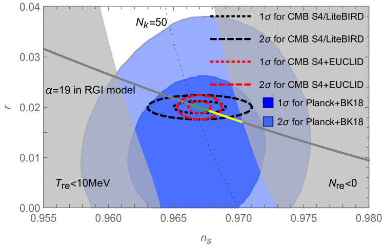
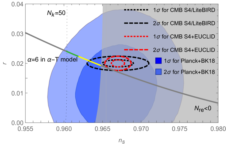
Figure 1: The diagonal line represents choices of $n_{s}$ and $r$ predicted by the RGI model (upper panel) and $\alpha$-T model (lower panel), with $X$ varying along the curve. Conditions  (3)- (5) are fulfilled in the green part, the gray parts are ruled out by the conditions $N_{\rm re}>0$ and $N_{\rm k}>50$. Ellipses indicate current constraints and future sensitivities to $n_{s}$ and $r$.

CMB constraints on the inflaton coupling

With the above considerations and the relations given in the appendix $N_{\rm k}$, $n_{s}$ and $r$ in a given model of inflation are all simple functions of $X\equiv\log_{10}\mathsf{g}$. Prior to any measurement of $n_{s}$ or $r$ the observed overall homogeneity and isotropy of the universe implies $N_{\rm k}>50$, and obviously $N_{\rm re}>0$. This translates into the probability density function (PDF)

$$P(X)=c_{1}P\big{(}N_{k}(X)\big{)}\ \gamma(X)\ \theta\big{(}N_{\rm re}(X)\big{)},$$ (10)

with $P(N_{k})\propto\frac{1}{2}\big{(}{\rm tanh}(N_{k}-50)+1\big{)}$, $\theta$ the Heaviside function, and $\gamma$ a function that allows for a re-weighting of the prior $P(X)$. The constant $c_{1}$ can be fixed from the requirement $\int_{D}dXP(X)=1$ where the integration domain is to be fixed by the condition $N_{\rm re}>0$ and the requirement to reheat the universe before big bang nucleosynthesis (BBN), i.e., $T_{\rm re}>T_{\rm BBN}$, which parametrically translates into Drewes (2019)

$$\mathsf{g}>g_{*}^{1/4}\frac{T_{\rm BBN}}{\sqrt{m_{\phi}M_{pl}}}\sqrt{\#}\simeq\frac{T_{\rm BBN}}{M_{pl}}\left(\frac{g_{*}}{A_{s}r}\right)^{1/4}\sqrt{\#}.$$ (11)

We now quantify the gain in knowledge about $X$ that can be obtained from data $\mathcal{D}$. Using $P(X)$ as prior, the gain in knowledge about $X$ can be quantified by the posterior distribution $P(X|\mathcal{D})=P(\mathcal{D}|X)P(X)/P(\mathcal{D})$ with $P(\mathcal{D})=\int dXP(\mathcal{D}|X)P(X)$. For the present purpose current constraints from the data $\mathcal{D}$ obtained by Planck and BICEP/Keck Ade et al. (2021) can be approximated by a two-dimensional Gaussian $\mathcal{N}(n_{s},r|\bar{n}_{s},\sigma_{n_{s}};\bar{r},\sigma_{r})$ to define the likelihood function

$$P(\mathcal{D}|X)=c_{2}\mathcal{N}(n_{s},r|\bar{n}_{s},\sigma_{n_{s}};\bar{r},\sigma_{r})\theta(r)\tilde{\gamma}(X),$$ (12)

with $\tilde{\gamma}$ another weighting function and the constant $c_{2}$ is fixed by normalising $P(\mathcal{D}|X)$ to unity. We fit the mean values $\bar{n}_{s}=0.967$, $\bar{r}=0.01$ and variances $\sigma_{n_{s}}=0.005$, $\sigma_{r}=0.016$ based on figure 5 in Ade et al. (2021). The result is shown in Fig. 2. For both models considered here, current CMB observations do not provide enough information in addition to the knowledge about $N_{\rm k}$ encoded in the prior  (10) to rule out a sizeable range of $X$ or $T_{\rm re}$. The scalar-to-tensor ratio will be constrained with much higher accuracy in the future Kamionkowski and Kovetz (2016). To quantify the expected information gain on $X$ we repeat the analysis, but assume $\bar{r}=0.02$ and use $\sigma_{n_{s}}=0.002$ and $\sigma_{r}=0.0012$, which corresponds to the sensitivity anticipated by LiteBIRD Allys et al. (2022) or CMB S4 Abazajian et al. (2022). Fig. 2 shows that in both models future data can rule out previously allowed values of $T_{\rm re}$. In the $\alpha{\rm-T}$ model the posterior peaks in a region where condition  (4) is violated, implying that $\Gamma$ depends on a potentially large number of model parameters $\{\mathsf{x}_{i}\}$ in a non-linear way, and it is impossible to translate a constraint on $N_{\rm re}$ into a model-independent constraint on $\mathsf{g}$. This is a result of the fact that the currently allowed region in Fig. 1 is very close to the $N_{\rm re}=0$ line. In the RGI model, on the other hand, the posterior peaks in a region where conditions  (3)- (5) are fulfilled, so that future CMB data will permit constraining the inflaton coupling. For the parameters chosen here, the mean values and variances for the prior and posteriors read $X=-5.5\pm 1.7$. Finally, we estimate the improvement that can be made with data from the EUCLID satellite Laureijs et al. (2011) and Square Kilometre Array (SKA) Maartens et al. (2015) by using $\sigma_{n_{s}}=0.00085$ Sprenger et al. (2019). The resulting posteriors in Fig. 2 for the chosen values of $\bar{n}_{s}$ and $\bar{r}$ impose a lower bound $T_{\rm re}>10^{14}$ GeV in the $\alpha$-T model. In the RGI model they allow for measurements $\log_{10}T_{\rm re}=8.8\pm 1.2$ GeV and $X=-6.1\pm 1.2$.

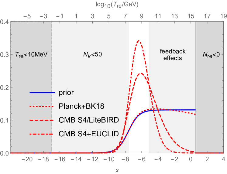
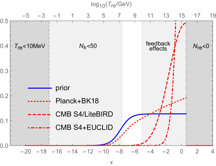
Figure 2: Prior $P(X)$ and posteriors $P(X|\mathcal{D})$ for $X=\log_{10}\mathsf{g}$ with the different choices of $\bar{n}_{s}$, $\bar{r}$, $\sigma_{n_{s}}$, and $\sigma_{r}$ in the RGI model (upper panel) and $\alpha$-T model (lower panel). We assumed $\gamma=\tilde{\gamma}=1$, but checked that the conclusions remain unchanged when using $\gamma=N_{\rm k}^{\prime}$ or $\tilde{\gamma}=(n_{s}^{{}^{\prime}2}+r^{{}^{\prime}2})^{1/2}$, with ^′ indicating a derivative with respect to $X$.

Conclusions

We quantified the information on the inflaton coupling and the reheating temperature that can be derived from the constraints on $n_{s}$ and $r$ obtained from the combined WMAP, Planck, and BICEP/Keck data. We also for the first time estimated the information gain that will be achieved with future observations, assuming a sensitivity to $r$ that LiteBIRD and CMB S4 aim for and a sensitivity to $n_{s}$ that can be achieved with EUCLID. In the two specific models that we studied we find that current data does not rule out a wide range of values for $\mathsf{g}$ and $T_{\rm re}$ in addition to the bounds which can be obtained from the requirement that inflation lasts long enough to explain the overall homogeneity and isotropy of the CMB. However, future CMB observations with LiteBIRD and CMB S4 will constrain $r$ sufficiently strongly to rule out sizeable ranges of $T_{\rm re}$ in both models. In the $\alpha{\rm-T}$ model the posterior peaks in a parameter region where feedback effects make it impossible to derive a particle physics model-independent bound on $X$, but we can still obtain a lower bound $T_{\rm re}>10^{14}$ GeV. In the RGI model this would, for the parameters we consider, allow to "measure" the inflaton coupling as $X=-5.5\pm 1.7$, with further improvement to $X=-6.1\pm 1.2$ when including data from EUCLID. Adding information from EUCLID and SKA on $n_{s}$ can, in addition to reducing the error bar on $X$, help to break parameter degeneracies and constrain $\alpha$ and $X$ simultaneously from data. The inflaton coupling did not only crucially shape the evolution of the observable universe through its impact on $T_{\rm re}$, but it is also a key parameter that connects models of inflation to theories of particle physics. Obtaining information on this microphysical parameter, even with large error bars, will represent an important achievement in particle cosmology, and provide an important clue to understand how a given model of inflation is embedded into a more fundamental theory of nature.

Appendix: Relation to observables

In this appendix we give the relations between the RHS of  (2) and observables. A detailed derivation can be found in Ueno and Yamamoto (2016) and has been adapted to our notation in Drewes et al. (2017). $N_{\rm re}$ can be obtained from

$$N_{\rm re} = \frac{4}{3\bar{w}_{\rm re}-1}\bigg{[}N_{\rm k}+\ln\left(\frac{k}{a_{0}T_{0}}\right)+\frac{1}{4}\ln\left(\frac{40}{\pi^{2}g_{*}}\right)$$

$$+\frac{1}{3}\ln\left(\frac{11g_{s*}}{43}\right)-\frac{1}{2}\ln\left(\frac{\pi^{2}M^{2}_{pl}rA_{s}}{2\sqrt{\mathcal{V}_{\rm end}}}\right)\bigg{]},$$

with $a_{0}$ and $T_{0}=2.725~{}{\rm K}$ the scale factor and the temperature of the CMB at the present time, respectively, and $N_{\rm k}$ is the number of $e$-folds between the horizon crossing of a perturbation with wave number $k$ and the end of inflation,

$$N_{\rm k}=\ln\left(\frac{a_{\rm end}}{a_{k}}\right)=\int_{\varphi_{k}}^{\varphi_{\rm end}}\frac{Hd\varphi}{\dot{\varphi}}\approx\frac{1}{M^{2}_{pl}}\int_{\varphi_{\rm end}}^{\varphi_{k}}d\varphi\frac{\mathcal{V}}{\partial_{\varphi}\mathcal{V}}~{}.$$ (14)

The subscript notation $H_{k},\varphi_{k}$ etc. indicates the value of the quantities $H,\varphi$ etc. at the moment when a pivot-scale $k$ crosses the horizon. $\varphi_{k}$ can be expressed in terms of the spectral index $n_{s}$ and the tensor-to-scalar ratio $r$ by solving the relations

$$n_{s}=1-6\epsilon_{k}+2\eta_{k}~{},\quad r=16\epsilon_{k}$$ (15)

with the slow roll parameters $\epsilon=\left(\partial_{\varphi}\mathcal{V}/\mathcal{V}\right)^{2}M^{2}_{pl}/2$ and $\eta=M^{2}_{pl}\partial^{2}_{\varphi}\mathcal{V}/\mathcal{V}$. In the slow roll regime, we find

$$H^{2}_{k}=\frac{\mathcal{V}(\varphi_{k})}{3M_{pl}^{2}}~{}=\pi^{2}M_{pl}^{2}\frac{rA_{s}}{2}$$ (16)

with $A_{s}=10^{-10}e^{3.043}$ Aghanim et al. (2020) the amplitude of the scalar perturbations from the CMB. $T_{\rm re}$ can be expressed in terms of the observables $(n_{s},A_{s},r)$ by plugging  (Appendix: Relation to observables) with  (14) into  (1), $\varphi_{k}$ is found by solving  (15) for $\varphi_{k}$, and $\mathcal{V}_{\rm end}$, and $\varphi_{\rm end}$ can be determined by solving $\epsilon=1$ for $\varphi$. From  (15) we obtain

$$\epsilon_{k}=\frac{r}{16}~{},\quad\eta_{k}=\frac{n_{s}-1+3r/8}{2},$$ (17)

from which we find

$$\frac{\partial_{\varphi}\mathcal{V}(\varphi)}{\mathcal{V}(\varphi)}\Bigl{|}_{\varphi_{k}}=\sqrt{\frac{r}{8M_{pl}^{2}}},\ \frac{\partial^{2}_{\varphi}\mathcal{V}(\varphi)}{\mathcal{V}(\varphi)}\Bigl{|}_{\varphi_{k}}=\frac{n_{s}-1+3r/8}{2M_{pl}^{2}}\quad$$ (18)

by using the definitions of $\epsilon$ and $\eta$. Together with  (16) this provides three equations that can be used to relate the effective potential and its derivatives to the observables $(n_{s},A_{s},r)$. That is sufficient to express $\bar{w}_{\rm re}$ and $N_{\rm re}$ in  (Appendix: Relation to observables) in terms of observables, which is all that is needed to determine the RHS of  (2).

References

- Aghanim et al. (2020) N. Aghanim et al. (Planck), Astron. Astrophys. 641, A6 (2020), [Erratum: Astron.Astrophys. 652, C4 (2021)], arXiv:1807.06209 [astro-ph.CO] .
- Ade et al. (2021) P. A. R. Ade et al. (BICEP, Keck), Phys. Rev. Lett. 127, 151301 (2021), arXiv:2110.00483 [astro-ph.CO] .
- Abdalla et al. (2022) E. Abdalla et al., JHEAp 34, 49 (2022), arXiv:2203.06142 [astro-ph.CO] .
- Giudice (2008) G. F. Giudice, , 155 (2008), arXiv:0801.2562 [hep-ph] .
- Workman (2022) R. L. Workman (Particle Data Group), PTEP 2022, 083C01 (2022).
- Canetti et al. (2012) L. Canetti, M. Drewes, and M. Shaposhnikov, New J. Phys. 14, 095012 (2012), arXiv:1204.4186 [hep-ph] .
- Starobinsky (1980) A. A. Starobinsky, Phys. Lett. B 91, 99 (1980).
- Guth (1981) A. H. Guth, Phys. Rev. D 23, 347 (1981).
- Linde (1982) A. D. Linde, Phys. Lett. B 108, 389 (1982).
- Martin et al. (2014a) J. Martin, C. Ringeval, and V. Vennin, Phys. Dark Univ. 5-6, 75 (2014a), arXiv:1303.3787 [astro-ph.CO] .
- Albrecht et al. (1982) A. Albrecht, P. J. Steinhardt, M. S. Turner, and F. Wilczek, Phys. Rev. Lett. 48, 1437 (1982).
- Dolgov and Kirilova (1990) A. D. Dolgov and D. P. Kirilova, Sov. J. Nucl. Phys. 51, 172 (1990).
- Traschen and Brandenberger (1990) J. H. Traschen and R. H. Brandenberger, Phys. Rev. D 42, 2491 (1990).
- Shtanov et al. (1995) Y. Shtanov, J. H. Traschen, and R. H. Brandenberger, Phys. Rev. D 51, 5438 (1995), arXiv:hep-ph/9407247 .
- Kofman et al. (1994) L. Kofman, A. D. Linde, and A. A. Starobinsky, Phys. Rev. Lett. 73, 3195 (1994), arXiv:hep-th/9405187 .
- Boyanovsky et al. (1996) D. Boyanovsky, H. J. de Vega, R. Holman, and J. F. J. Salgado, Phys. Rev. D 54, 7570 (1996), arXiv:hep-ph/9608205 .
- Kofman et al. (1997) L. Kofman, A. D. Linde, and A. A. Starobinsky, Phys. Rev. D 56, 3258 (1997), arXiv:hep-ph/9704452 .
- Caprini and Figueroa (2018) C. Caprini and D. G. Figueroa, Class. Quant. Grav. 35, 163001 (2018), arXiv:1801.04268 [astro-ph.CO] .
- Martin and Ringeval (2010) J. Martin and C. Ringeval, Phys. Rev. D 82, 023511 (2010), arXiv:1004.5525 [astro-ph.CO] .
- Adshead et al. (2011) P. Adshead, R. Easther, J. Pritchard, and A. Loeb, JCAP 02, 021 (2011), arXiv:1007.3748 [astro-ph.CO] .
- Easther and Peiris (2012) R. Easther and H. V. Peiris, Phys. Rev. D 85, 103533 (2012), arXiv:1112.0326 [astro-ph.CO] .
- Martin et al. (2015) J. Martin, C. Ringeval, and V. Vennin, Phys. Rev. Lett. 114, 081303 (2015), arXiv:1410.7958 [astro-ph.CO] .
- Munoz and Kamionkowski (2015) J. B. Munoz and M. Kamionkowski, Phys. Rev. D 91, 043521 (2015), arXiv:1412.0656 [astro-ph.CO] .
- Cook et al. (2015) J. L. Cook, E. Dimastrogiovanni, D. A. Easson, and L. M. Krauss, JCAP 04, 047 (2015), arXiv:1502.04673 [astro-ph.CO] .
- Zhang et al. (2020) N. Zhang, Y.-B. Wu, J.-W. Lu, C.-W. Sun, L.-J. Shou, and H.-Z. Xu, Chin. Phys. C 44, 095107 (2020), arXiv:1807.03596 [astro-ph.CO] .
- Stein and Kinney (2022) N. K. Stein and W. H. Kinney, JCAP 01, 022 (2022), arXiv:2106.02089 [astro-ph.CO] .
- Cai et al. (2015) R.-G. Cai, Z.-K. Guo, and S.-J. Wang, Phys. Rev. D 92, 063506 (2015), arXiv:1501.07743 [gr-qc] .
- Di Marco et al. (2018) A. Di Marco, G. Pradisi, and P. Cabella, Phys. Rev. D 98, 123511 (2018), arXiv:1807.05916 [astro-ph.CO] .
- Maity and Saha (2019a) D. Maity and P. Saha, JCAP 07, 018 (2019a), arXiv:1811.11173 [astro-ph.CO] .
- Maity and Saha (2019b) D. Maity and P. Saha, Class. Quant. Grav. 36, 045010 (2019b), arXiv:1902.01895 [gr-qc] .
- Antusch et al. (2020) S. Antusch, D. G. Figueroa, K. Marschall, and F. Torrenti, Phys. Lett. B 811, 135888 (2020), arXiv:2005.07563 [astro-ph.CO] .
- Dai et al. (2014) L. Dai, M. Kamionkowski, and J. Wang, Phys. Rev. Lett. 113, 041302 (2014), arXiv:1404.6704 [astro-ph.CO] .
- Domcke and Heisig (2015) V. Domcke and J. Heisig, Phys. Rev. D 92, 103515 (2015), arXiv:1504.00345 [astro-ph.CO] .
- Dalianis et al. (2017) I. Dalianis, G. Koutsoumbas, K. Ntrekis, and E. Papantonopoulos, JCAP 02, 027 (2017), arXiv:1608.04543 [gr-qc] .
- Takahashi and Yin (2019) F. Takahashi and W. Yin, JHEP 07, 095 (2019), arXiv:1903.00462 [hep-ph] .
- Hardwick et al. (2016) R. J. Hardwick, V. Vennin, K. Koyama, and D. Wands, JCAP 08, 042 (2016), arXiv:1606.01223 [astro-ph.CO] .
- Ueno and Yamamoto (2016) Y. Ueno and K. Yamamoto, Phys. Rev. D 93, 083524 (2016), arXiv:1602.07427 [astro-ph.CO] .
- Nozari and Rashidi (2017) K. Nozari and N. Rashidi, Phys. Rev. D 95, 123518 (2017), arXiv:1705.02617 [astro-ph.CO] .
- Di Marco et al. (2017) A. Di Marco, P. Cabella, and N. Vittorio, Phys. Rev. D 95, 103502 (2017), arXiv:1705.04622 [astro-ph.CO] .
- Drewes et al. (2017) M. Drewes, J. U. Kang, and U. R. Mun, JHEP 11, 072 (2017), arXiv:1708.01197 [astro-ph.CO] .
- Maity and Saha (2018) D. Maity and P. Saha, Phys. Rev. D 98, 103525 (2018), arXiv:1801.03059 [hep-ph] .
- Rashidi and Nozari (2018) N. Rashidi and K. Nozari, Int. J. Mod. Phys. D 27, 1850076 (2018), arXiv:1802.09185 [astro-ph.CO] .
- Mishra et al. (2021) S. S. Mishra, V. Sahni, and A. A. Starobinsky, JCAP 05, 075 (2021), arXiv:2101.00271 [gr-qc] .
- Ellis et al. (2022) J. Ellis, M. A. G. Garcia, D. V. Nanopoulos, K. A. Olive, and S. Verner, Phys. Rev. D 105, 043504 (2022), arXiv:2112.04466 [hep-ph] .
- Nautiyal (2018) A. Nautiyal, Phys. Rev. D 98, 103531 (2018), arXiv:1806.03081 [astro-ph.CO] .
- Choi and Lee (2016) S.-M. Choi and H. M. Lee, Eur. Phys. J. C 76, 303 (2016), arXiv:1601.05979 [hep-ph] .
- Cabella et al. (2017) P. Cabella, A. Di Marco, and G. Pradisi, Phys. Rev. D 95, 123528 (2017), arXiv:1704.03209 [astro-ph.CO] .
- Kabir et al. (2019) R. Kabir, A. Mukherjee, and D. Lohiya, Mod. Phys. Lett. A 34, 1950114 (2019), arXiv:1609.09243 [gr-qc] .
- Bhattacharya et al. (2017) S. Bhattacharya, K. Dutta, and A. Maharana, Phys. Rev. D 96, 083522 (2017), [Addendum: Phys.Rev.D 96, 109901 (2017)], arXiv:1707.07924 [hep-ph] .
- Dalianis and Watanabe (2018) I. Dalianis and Y. Watanabe, JHEP 02, 118 (2018), arXiv:1801.05736 [hep-ph] .
- Drewes (2016) M. Drewes, JCAP 03, 013 (2016), arXiv:1511.03280 [astro-ph.CO] .
- Moncelsi et al. (2020) L. Moncelsi et al., Proc. SPIE Int. Soc. Opt. Eng. 11453, 1145314 (2020), arXiv:2012.04047 [astro-ph.IM] .
- Ade et al. (2019) P. Ade et al. (Simons Observatory), JCAP 02, 056 (2019), arXiv:1808.07445 [astro-ph.CO] .
- Allys et al. (2022) E. Allys et al. (LiteBIRD), (2022), arXiv:2202.02773 [astro-ph.IM] .
- Abazajian et al. (2022) K. Abazajian et al. (CMB-S4), Astrophys. J. 926, 54 (2022), arXiv:2008.12619 [astro-ph.CO] .
- Martin et al. (2016) J. Martin, C. Ringeval, and V. Vennin, Phys. Rev. D 94, 123521 (2016), arXiv:1609.04739 [astro-ph.CO] .
- Renaux-Petel and Turzyński (2016) S. Renaux-Petel and K. Turzyński, Phys. Rev. Lett. 117, 141301 (2016), arXiv:1510.01281 [astro-ph.CO] .
- Passaglia et al. (2021) S. Passaglia, W. Hu, A. J. Long, and D. Zegeye, Phys. Rev. D 104, 083540 (2021), arXiv:2108.00962 [hep-ph] .
- Drewes (2019) M. Drewes, (2019), arXiv:1903.09599 [astro-ph.CO] .
- Amin et al. (2014) M. A. Amin, M. P. Hertzberg, D. I. Kaiser, and J. Karouby, Int. J. Mod. Phys. D 24, 1530003 (2014), arXiv:1410.3808 [hep-ph] .
- Fairbairn et al. (2003) M. Fairbairn, L. Lopez Honorez, and M. H. G. Tytgat, Phys. Rev. D 67, 101302 (2003), arXiv:hep-ph/0302160 .
- Martin et al. (2014b) J. Martin, C. Ringeval, R. Trotta, and V. Vennin, JCAP 03, 039 (2014b), arXiv:1312.3529 [astro-ph.CO] .
- Kallosh and Linde (2013a) R. Kallosh and A. Linde, JCAP 10, 033 (2013a), arXiv:1307.7938 [hep-th] .
- Kallosh and Linde (2013b) R. Kallosh and A. Linde, JCAP 07, 002 (2013b), arXiv:1306.5220 [hep-th] .
- Carrasco et al. (2015a) J. J. M. Carrasco, R. Kallosh, and A. Linde, JHEP 10, 147 (2015a), arXiv:1506.01708 [hep-th] .
- Carrasco et al. (2015b) J. J. M. Carrasco, R. Kallosh, and A. Linde, Phys. Rev. D 92, 063519 (2015b), arXiv:1506.00936 [hep-th] .
- Boyanovsky et al. (2005) D. Boyanovsky, K. Davey, and C. M. Ho, Phys. Rev. D 71, 023523 (2005), arXiv:hep-ph/0411042 .
- Drewes and Kang (2013) M. Drewes and J. U. Kang, Nucl. Phys. B 875, 315 (2013), [Erratum: Nucl.Phys.B 888, 284–286 (2014)], arXiv:1305.0267 [hep-ph] .
- Carenza et al. (2020) P. Carenza, A. Mirizzi, and G. Sigl, Phys. Rev. D 101, 103016 (2020), arXiv:1911.07838 [hep-ph] .
- Kamionkowski and Kovetz (2016) M. Kamionkowski and E. D. Kovetz, Ann. Rev. Astron. Astrophys. 54, 227 (2016), arXiv:1510.06042 [astro-ph.CO] .
- Laureijs et al. (2011) R. Laureijs et al. (EUCLID), (2011), arXiv:1110.3193 [astro-ph.CO] .
- Maartens et al. (2015) R. Maartens, F. B. Abdalla, M. Jarvis, and M. G. Santos (SKA Cosmology SWG), PoS AASKA14, 016 (2015), arXiv:1501.04076 [astro-ph.CO] .
- Sprenger et al. (2019) T. Sprenger, M. Archidiacono, T. Brinckmann, S. Clesse, and J. Lesgourgues, JCAP 02, 047 (2019), arXiv:1801.08331 [astro-ph.CO] .