An Optimal Transport Approach to
   the Computation of the LM Rate

Abstract

Mismatch capacity characterizes the highest information rate for a channel under a prescribed decoding metric, and is thus a highly relevant fundamental performance metric when dealing with many practically important communication scenarios. Compared with the frequently used generalized mutual information (GMI), the LM rate has been known as a tighter lower bound of the mismatch capacity. The computation of the LM rate, however, has been a difficult task, due to the fact that the LM rate involves a maximization over a function of the channel input, which becomes challenging as the input alphabet size grows, and direct numerical methods (e.g., interior point methods) suffer from intensive memory and computational resource requirements. Noting that the computation of the LM rate can also be formulated as an entropy-based optimization problem with constraints, in this work, we transform the task into an optimal transport (OT) problem with an extra constraint. This allows us to efficiently and accurately accomplish our task by using the well-known Sinkhorn algorithm. Indeed, only a few iterations are required for convergence, due to the fact that the formulated problem does not contain additional regularization terms. Moreover, we convert the extra constraint into a root-finding procedure for a one-dimensional monotonic function. Numerical experiments demonstrate the feasibility and efficiency of our OT approach to the computation of the LM rate.

I Introduction

The Shannon capacity of a channel characterizes the ultimate transmission efficiency limit of reliable communication over a channel [2]. It has played a fundamental role in the research of communication theory and directed the development of communication systems for decades.

In many scenarios of practical interest, however, the perfect knowledge about a channel may not be available or may not be fully utilized for implementing the transceivers. Important examples include channels with uncertainty (like fading in wireless communication systems) [3], with non-ideal transceiver hardware [4], or with constrained receiver structure [5]. A commonly adopted practice of the receiver under such circumstances is to use a prescribed decoding metric, which may not be matched to the actual channel transition probability, and the mismatch capacity has been introduced to characterize the highest information rate under a prescribed decoding metric; see, e.g., [6] [7] and references therein.

Unfortunately, the mismatch capacity is still an open problem to date [8]. So instead of it, researchers have been focusing on deriving its achievable lower bounds. The generalized mutual information (GMI) is a relatively simple lower bound [9], which has found extensive applications in various setups; see, e.g., [3] [4] [10]. However, the LM rate [1] is a tighter lower bound, by replacing the independent and identically distributed (i.i.d.) codebook ensemble for the GMI by constant-composition codebook ensemble.

From the perspective of optimization, the primal forms of the GMI and the LM rate are highly similar, except that for the LM rate there is an additional constraint on the marginal distribution of the sought-for maximizing joint probability distribution over the input and output alphabets; see, e.g., [11, Thm. 1]. Consequently, the dual form of the GMI is easy to compute, since it can be written as a maximization over a real number [11, Eqn. (12)], which is readily solved by a one-dimensional line search. On the other hand, the dual form of the LM rate further involves a maximization over a function of the channel input [11, Eqn. (11)]. Consequently the computation of the LM rate is much more challenging, and there is rare work on the numerical computation of the LM rate. Interior point methods (e.g., [12, 13]) can be applied for computing the LM rate, but it is typically memory intensive and computationally expensive. It is therefore desirable to develop effective computation models and efficient numerical algorithms for the LM rate.

In this paper, we formulate the LM rate computation as an optimal transport (OT) problem with an extra constraint, motivated by the similarity between these two optimization problems. Our contribution consists of three parts. First, we propose an OT model with an extra constraint for the LM rate. Second, we show that this model can be solved directly using the well-known Sinkhorn algorithm [14]. Since our OT model is strongly convex, no additional regularization is required. This guarantees that we only need several hundred of Sinkhorn iterations to converge rather than tens of thousands of iterations for classical OT problems. Last, we show that the extra constraint in the OT problem formulation can be efficiently handled by finding the root of a one-dimensional monotone function, and the feasibility of the extra constraint is guaranteed at each iteration. Numerical experiments show that for the case of QPSK and 16-QAM, our proposed algorithm is efficient and accurate. We also point out that our method is highly scalable and can be easily generalized to large-scale cases, such as 256-QAM.

The remaining part of this paper is organized as follows. In Section II, after briefly reviewing the basic definition of the LM rate, we write it in the form of OT model with an extra constraint. Next, we present the numerical methods for this problem, including the Sinkhorn algorithm and the treatment of the extra constraint in Section III. In Section IV, the simulation results demonstrate the advantages of our approach. We finally conclude the paper in Section V.

II Problem Formulation

II-A The LM Rate

We consider a discrete memoryless communication channel model with transition law $W(y|x)$ over the (finite, discrete) channel input alphabet $\mathcal{X}=\{x_{1},\cdots,x_{M}\}\subset\mathbb{R}^{2}$ and the channel output alphabet $\mathcal{Y}\subset\mathbb{R}^{2}$. Thus, given a probability measure $P_{X}$ on $\mathcal{X}$, we are able to define the joint probability distribution $P_{XY}$ on $\mathcal{X}\times\mathcal{Y}$ and the output distribution $P_{Y}$ on $\mathcal{Y}$ by the following:

$$P_{XY}(x_{i},B)=W(B|x_{i})P_{X}(x_{i}),~{}\forall B\subset\mathcal{Y},$$

$$P_{Y}(B)=\sum_{i=1}^{M}W(B|x_{i})P_{X}(x_{i}),~{}\forall B\subset\mathcal{Y}.$$

This discrete memoryless channel is in fact a mapping from the input alphabet $\mathcal{X}$ to the output alphabet $\mathcal{Y}$ with the channel transition law $W(y|x)$.

For transmission of rate $R$, a block length-$n$ codebook $\mathcal{C}$ consists of $2^{nR}$ vectors $\mathbf{x}(m)=(x^{(1)}(m),\cdots,x^{(n)}(m))\in\mathcal{X}^{n}$. The encoder maps the message $m$ uniformly randomly selected from the set $\mathcal{M}=\{1,\cdots,2^{nR}\}$ to the corresponding codeword $\mathbf{x}(m)$. After receiving the output sequence $\mathbf{y}=(y^{(1)},\cdots,y^{(n)})$, the decoder forms the estimation on the message $m$ following the decoding rule

$$\hat{m}=\operatorname*{\arg\min}_{j\in\mathcal{M}}\sum_{k=1}^{n}d(x^{(k)}(j),y^{(k)}),$$

where $d:\mathcal{X}\times\mathcal{Y}\to\mathbb{R}$ is a non-negative function called the decoding metric.

With the notations defined above, the LM rate, as one of the achievable lower bound of the mismatch capacity, is defined as:

$$I_{LM}(P_{X}) :=\min_{{\color[rgb]{0,0,0}\gamma\in\mathcal{P}(\mathcal{X}\times\mathcal{Y})}}D(\gamma\|P_{X}P_{Y})$$ (1a)

$$\textrm{s.t.}\quad\int_{y\in\mathcal{Y}}\gamma(x_{i},y)\mathrm{d}y =P_{X}(x_{i}),\ \forall x_{i}\in\mathcal{X},$$ (1b)

$$\sum_{x_{i}\in\mathcal{X}}\gamma(x_{i},y) =P_{Y}(y),\ \forall y\in\mathcal{Y},$$ (1c)

$$\int_{y\in\mathcal{Y}}\sum_{x_{i}\in\mathcal{X}}\gamma d(x_{i},y)\mathrm{d}y \leq\int_{y\in\mathcal{Y}}\sum_{x_{i}\in\mathcal{X}}P_{XY}d(x_{i},y)\mathrm{d}y.$$ (1d)

Here $D(\cdot\|\cdot)$ denotes the relative entropy function and $\mathcal{P}(\mathcal{X}\times\mathcal{Y})$ denotes the set of all joint probability distributions on $\mathcal{X}\times\mathcal{Y}$.

II-B The OT Problem

In (1), we can see that the LM rate is similar to the OT problem [15] in terms of optimization objective and constraints. Naturally, we would like to derive an equivalent OT-type problem to (1), which creates a prerequisite for computing the LM rate by using the Sinkhorn algorithm [14].

Consider a discrete probability distribution $\mu_{i}=P_{X}(x_{i})$ on $\mathcal{X}$. It satisfies the following normalization and average power constraints:

$$\sum_{i=1}^{M}\mu_{i}=1,\quad\sum_{i=1}^{M}\mu_{i}\|x_{i}\|_{2}^{2}=1.$$ (2)

For given channel transition law $W(y|x)$ and decoding metric $d(x,y)$, the right-hand side of (1d) is a constant:

$$T =\int_{\mathcal{Y}}\sum_{i=1}^{M}P_{XY}(x_{i},y)d(x_{i},y)\mathrm{d}y$$ (3)

$$=\int_{\mathcal{Y}}\sum_{i=1}^{M}\mu_{i}W(y|x_{i})d(x_{i},y)\mathrm{d}y.$$

Moreover, it is easy to show that

$$D(\gamma\|P_{X}P_{Y})=\int_{\mathcal{Y}}\sum_{i=1}^{M}\gamma(x_{i},y)\log\gamma(x_{i},y)\mathrm{d}y-C,$$

$$C=\sum_{i=1}^{M}P_{X}(x_{i})\log P_{X}(x_{i})+\int_{\mathcal{Y}}P_{Y}(y)\log P_{Y}(y)\mathrm{d}y.$$

By neglecting the constant $C$, minimizing the objective function $D(\gamma\|P_{X}P_{Y})$ is equivalent to maximizing the entropy

$$-\int_{\mathcal{Y}}\sum_{i=1}^{M}\gamma(x_{i},y)\log\gamma(x_{i},y)\mathrm{d}y.$$

Thus, we have obtained the following optimal transport problem (4a)-(4c) with an extra constraint (4d):

$$\min_{{\color[rgb]{0,0,0}\gamma\in\mathcal{P}(\mathcal{X}\times\mathcal{Y})}} \int_{\mathcal{Y}}\sum_{i=1}^{M}\gamma(x_{i},y)\log\gamma(x_{i},y)\mathrm{d}y$$ (4a)

s.t. $$\int_{\mathcal{Y}}\gamma(x_{i},y)\mathrm{d}y=\mu_{i},\quad i=1,\cdots,M,$$ (4b)

$$\sum_{i=1}^{M}\gamma(x_{i},y)=P_{Y}(y),\quad\forall y\in\mathcal{Y},$$ (4c)

$$\int_{\mathcal{Y}}\sum_{i=1}^{M}\gamma(x_{i},y)d(x_{i},y)\mathrm{d}y\leq T.$$ (4d)

Remark 1

In the classical OT theory, the cost function is only related to distance and should be independent of variables. Thus, (4a)-(4d) is not a standard OT form, since the “cost function” $\log\gamma(x_{i},y)$ in (4a) is related to the variables $\gamma(x_{i},y)$. However, the optimization objective function (4a) is obtained by complicated and lengthy inequality scaling of the original problem (2.29) in [7], which is in standard OT form. For detailed derivation, the interested readers are referred to Chapter 2 in [16]. On the other hand, from the numerical point of view, the optimization problem (4a)-(4d) can be efficiently solved by the Sinkhorn algorithm, which is well-known for its high efficiency in solving OT problems. In these senses, we might as well call (4a)-(4d) an OT problem.

III THE Sinkhorn ALGORITHM

In this section, we turn to the Sinkhorn algorithm for the equivalent OT problem to the LM rate. First, we need to discretize the integral in (4). We might as well consider a set of uniform grid points $\{y_{j}\}_{j=1}^{N}$ in $\mathcal{Y}$, and the corresponding rectangular discretization of the integral. This leads to the discrete form of (4):

$$\min_{{\color[rgb]{0,0,0}\gamma_{ij}}}\quad \sum_{i=1}^{M}\sum_{j=1}^{N}\gamma_{ij}\log\gamma_{ij}$$ (5a)

s.t. $$\sum_{j=1}^{N}\gamma_{ij}=\mu_{i},\quad i=1,\cdots,M,$$ (5b)

$$\sum_{i=1}^{M}\gamma_{ij}=\nu_{j},\quad j=1,\cdots,N,$$ (5c)

$$\sum_{i=1}^{M}\sum_{j=1}^{N}d_{ij}\gamma_{ij}\leq T.$$ (5d)

Here $\gamma_{ij}=\gamma(x_{i},y_{j}),\;\nu_{j}=P_{Y}(y_{j})$ and $d_{ij}=d(x_{i},y_{j})$.

Remark 2

In this work, we illustrate our key idea through the rectangular formula with only first-order accuracy for numerical integration. The idea can be easily generalized to a higher-order numerical discretization, e.g., the trapezoid formula. Not only that, the Sinkhorn algorithm, which we will discuss later in this section, only requires minor modifications to be suitable for higher-order discretization.

Introducing the dual variables $\bm{\alpha}\in\mathbb{R}^{M},\bm{\beta}\in\mathbb{R}^{N}$ and $\lambda\in\mathbb{R}^{+}$, the Lagrangian of (5) can be written as:

$$\mathcal{L}(\gamma;\bm{\alpha},\bm{\beta},\lambda)=\sum_{i=1}^{M}\sum_{j=1}^{N}\gamma_{ij}\log\gamma_{ij}+\sum_{i=1}^{M}\alpha_{i}(\sum_{j=1}^{N}\gamma_{ij}-\mu_{i})$$ (6)

$$+\sum_{j=1}^{N}\beta_{j}(\sum_{i=1}^{M}\gamma_{ij}-\nu_{j})+\lambda(\sum_{i=1}^{M}\sum_{j=1}^{N}d_{ij}\gamma_{ij}-T).$$

Taking the derivative of $\mathcal{L}(\gamma;\bm{\alpha},\bm{\beta},\lambda)$ with respect to $\gamma_{ij}$ leads to

$$\gamma_{ij}=\phi_{i}\Lambda_{ij}\psi_{j},$$

in which

$$\phi_{i}=\mathrm{e}^{-\alpha_{i}-1/2},\;\psi_{j}=\mathrm{e}^{-\beta_{j}-1/2},\;\Lambda_{ij}=\mathrm{e}^{-\lambda d_{ij}}.$$

Substituting the above formula into (5b) and (5c) yields

$$\phi_{i}\sum_{j=1}^{N}\Lambda_{ij}\psi_{j}=\mu_{i},\quad i=1,\cdots,M,$$

$$\psi_{j}\sum_{i=1}^{M}\Lambda_{ij}\phi_{i}=\nu_{j},\quad j=1,\cdots,N.$$

Since $\Lambda_{ij}>0$, we can alternatively update $\phi_{i}$ and $\psi_{j}$ as follows:

$$\phi_{i}^{(\ell+1)}=\mu_{i}/\sum_{j=1}^{N}\Lambda_{ij}^{(\ell)}\psi_{j}^{(\ell)},\quad i=1,\cdots,M,$$ (7a)

$$\psi_{j}^{(\ell+1)}=\nu_{j}/\sum_{i=1}^{M}\Lambda_{ij}^{(\ell)}\phi_{i}^{(\ell+1)},\quad j=1,\cdots,N.$$ (7b)

This iterative formula is the well-known Sinkhorn algorithm [17]. Different from the classical OT problem, we need to deal with the extra constraint (5d). By taking the derivative of $\mathcal{L}(\gamma;\bm{\alpha},\bm{\beta},\lambda)$ with respect to $\lambda$, we have

$$G(\lambda)\triangleq\sum_{i=1}^{M}\sum_{j=1}^{N}\phi_{i}\psi_{j}d_{ij}\mathrm{e}^{-\lambda d_{ij}}-T=0.$$ (8)

Thus, we can update $\lambda$ by finding the roots of

$$G(\lambda^{(\ell+1)})\triangleq\sum_{i=1}^{M}\sum_{j=1}^{N}\phi_{i}^{(\ell+1)}\psi_{j}^{(\ell+1)}d_{ij}\mathrm{e}^{-\lambda^{(\ell+1)}d_{ij}}-T.$$

Noticing that

$$G^{\prime}(\lambda)=-\sum_{i=1}^{M}\sum_{j=1}^{N}\phi_{i}\psi_{j}d_{ij}^{2}\mathrm{e}^{-\lambda d_{ij}}<0,$$

the function $G(\lambda)$ is monotonic. Thus, The problem of finding the root of $G(\lambda)$ can be easily solved by the Newton’s method. The pseudo-code of the proposed algorithm is present in Algorithm 1.

Algorithm 1 The Sinkhorn Algorithm

0:  Decoding metric $d_{ij}$; Marginal distributions $\mu_{i},\nu_{j}$; Iteration number $K$.

0:  Minimal value of $\sum_{i=1}^{M}\sum_{j=1}^{N}\gamma_{ij}\log\gamma_{ij}$.

1:  Initialization: $\bm{\phi}=\mathbf{1}_{M},\bm{\psi}=\mathbf{1}_{N},\lambda=1$;

2:  for $\ell=1:K$ do

3:     $\Lambda_{ij}\leftarrow\mathrm{e}^{-\lambda d_{ij}}$, $i=1,\cdots,M,\ j=1,\cdots,N$

4:     for $i=1:M$ do

5:        $\phi_{i}\leftarrow\mu_{i}/\sum_{j=1}^{N}\Lambda_{ij}\psi_{j}$

6:     for $j=1:N$ do

7:        $\psi_{j}\leftarrow\nu_{j}/\sum_{i=1}^{M}\Lambda_{ij}\phi_{i}$

8:     Solve $G(\lambda)=0$ for $\lambda$ with Newton’s method

9:  return  $\sum_{i=1}^{M}\sum_{j=1}^{N}\phi_{i}\psi_{j}\Lambda_{ij}\log\left(\phi_{i}\psi_{j}\Lambda_{ij}\right)$

Finally, we need to discuss the feasibility of the Sinkhorn iteration, especially under the extra constraint (5d). Depending on the value of $G(0)$, there are two cases:

• $G(0)>0$: In this case, $G(\lambda)=0$ has a unique solution on $(0,+\infty)$ since $G^{\prime}(\lambda)<0$. Thus the extra constraint (5d) is obviously satisfied.

• $G(0)\leq 0$: In this case, the extra constraint (5d) is already satisfied. We only need to set $\lambda=0$ instead of solving $G(\lambda)=0$ at line 8 of Algorithm 1.

IV NUMERICAL SIMULATIONS

In this section, we use the model and algorithm developed in previous sections to compute the LM rate for different modulation schemes over the additive white Gaussian noise (AWGN) channels subject to rotation and scaling with the following transition law

$$Y=HX+Z,\ \text{with }Z\sim\mathcal{N}(0,\sigma_{Z}^{2}).$$ (9)

The matrix $H\in\mathbb{R}^{2\times 2}$ is a combination of rotation and scaling transformations as

$$H=\begin{pmatrix}\eta_{1}&0\\ 0&\eta_{2}\end{pmatrix}\begin{pmatrix}\cos\theta&\sin\theta\\ -\sin\theta&\cos\theta\end{pmatrix}.$$

Here the parameters $\eta_{1},\;\eta_{2}$ indicate the scaling of the signal, and the parameter $\theta$ indicates the degree of rotation on the signal. In this work, we consider the case of $\eta_{1}=1$ and $\eta_{2}=\eta$. Note that, the specific values of $\eta$ and $\theta$ can not be priorly known.

The decoding metric is $d(x,y):=\|y-\hat{H}x\|_{2}^{2}$, where $\hat{H}$ is an approximation that is based on part of the information we know about $H$. We consider the scenario in which the decoder is unaware of the mismatch effect. Thus, in the decoding rule, we have $\hat{H}=I$.

In the following simulations, we consider two classical modulation schemes: QPSK and 16-QAM. Under the power constraint (2), their constellation points (also known as the alphabet) are illustrated in Fig 1. For both cases, all the constellation points in $\mathcal{X}$ are restricted in the region $[-1,1]\times[-1,1]$.

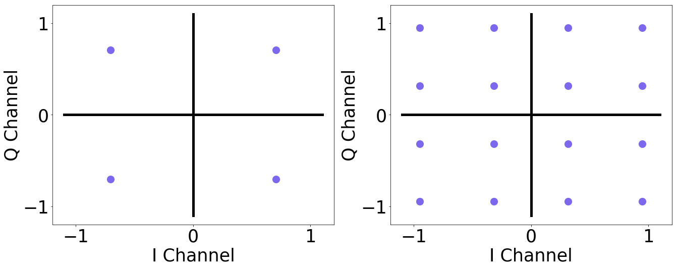
Figure 1: Constellation points under the power constraint. Left: The QPSK modulation scheme. Right: The 16-QAM modulation scheme.

Meanwhile, according to the channel law (9), the channel output alphabet $\mathcal{Y}$ is $\mathbb{R}^{2}$ itself. Under some reasonable assumptions, e.g. $\eta\leq 1,\sigma_{z}^{2}\leq\frac{1}{2}$, we are able to truncate the alphabet $\mathcal{Y}$ with a sufficiently large region, e.g. $[-8,8]\times[-8,8]$. Correspondingly, we can discretize the region by a set of uniform grid points $\{y_{j}\}_{j=1}^{N}$:

$$y_{r\sqrt{N}+s} =(-8+r\Delta y,-8+(s-1)\Delta y),\Delta y=\frac{16}{\sqrt{N}-1},$$

$$r =0,1,\cdots,\sqrt{N}-1,s=1,2,\cdots,\sqrt{N},$$

In Algorithm 1, the termination condition of the Newton iteration is that the update step size of $\lambda$ is less than $10^{-14}$. Moreover, the $\text{SNR}\triangleq 1/(2\sigma_{Z}^{2})$ is used in the sequel.

All the experiments are conducted on a platform with 128G RAM, and one Intel(R) Xeon(R) Gold 5117 CPU @2.00GHz with 14 cores.

IV-A Algorithm Verfication

We first study the convergence of our Sinkhorn algorithm by considering the residual errors of (7) and (8):

$$r_{\phi} =\sum_{i=1}^{M}|\phi_{i}\sum_{j=1}^{N}\Lambda_{ij}\psi_{j}-\mu_{i}|,$$

$$r_{\psi} =\sum_{j=1}^{N}|\psi_{j}\sum_{i=1}^{M}\Lambda_{ij}\phi_{i}-\nu_{j}|,$$

$$r_{\lambda} =|G(\lambda)|.$$

The parameters are set to

$$(\eta,\theta)=(0.9,\pi/18),\;N=250,000,\;\text{SNR}=0\textrm{dB}.$$ (10)

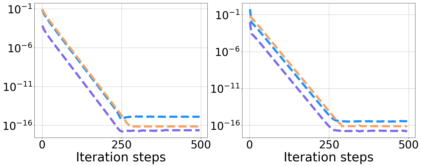
Figure 2: The convergent trajectories of the residual error for $r_{\phi}$ (Orange), $r_{\psi}$ (Blue) and $r_{\lambda}$ (Purple). Left: The QPSK modulation scheme. Right: The 16-QAM modulation scheme.

TABLE I: Comparison between the Sinkhorn algorithm and CVX. Columns 3-5 are the averaged computational time and the speed-up ratio of the Sinkhorn algorithm. Column 6 is the averaged difference of the LM rate computed by two methods.

	$N$	Computational time (s)		Speed-up ratio	Average difference
		Sinkhorn	CVX
QPSK	$100$	$0.37\times 10^{0}$	$2.61\times 10^{1}$	$7.05\times 10^{1}$	$1.99\times 10^{-7}$
	$225$	$0.64\times 10^{0}$	$8.66\times 10^{1}$	$1.35\times 10^{2}$	$6.45\times 10^{-7}$
	$400$	$1.28\times 10^{0}$	-	-	-
16-QAM	$100$	$0.96\times 10^{0}$	$1.49\times 10^{2}$	$1.55\times 10^{2}$	$4.13\times 10^{-7}$
	$225$	$1.96\times 10^{0}$	$9.27\times 10^{2}$	$4.73\times 10^{2}$	$1.37\times 10^{-6}$
	$400$	$3.81\times 10^{0}$	-	-	-
256-QAM	$100$	$1.49\times 10^{1}$	-	-	-
	$1600$	$2.24\times 10^{2}$	-	-	-

In Fig. 2, we output the convergent trajectories of the residual errors with respect to iteration steps. We can see that the three curves all decrease rapidly and reach the machine accuracy near $250$ iterations. It is worth mentioning that classical OT problems usually require tens of thousands of Sinkhorn iterations to converge. This significantly illustrates the dramatic efficiency advantage of our OT model and Sinkhorn algorithm.

To further illustrate the accuracy and efficiency of the Sinkhorn algorithm for the OT problem (5). We use CVX [13] as the baseline. The averaged computational time and the averaged difference of the optimal values between the two methods are listed in Table I. To reduce the influence of noise, we repeat each experiment for $100$ times. Except for $N$, other parameters are the same as (10). Since it is difficult for CVX to handle large-scale problems, we restrict $N$ to small scales, e.g. $100,\;225,\;400$ and $1600$. From the table, we can see the optimal values obtained by the two methods are almost the same. But our Sinkhorn algorithm has a significant advantage (one or two orders of magnitude) in computational speed. Moreover, for slightly larger scale problems, CVX has failed to output convergent results.

IV-B Results and Discussions

Below, we present the computational results of the LM rate under different modulation schemes, different parameters $(\eta,\theta)$, and different SNRs. For comparison, we also present the computational results of GMI [4] under the same setup. As we know, GMI is generally lower than the LM rate [7]. These results not only help us quantitatively understand the relationship between the two rates, but also help verify the correctness of our model and algorithm. In the numerical experiments, we consider four sets of parameters $(\eta,\theta)$, namely,

$$(0.9,\frac{\pi}{18}),\quad(0.9,\frac{\pi}{12}),\quad(0.8,\frac{\pi}{18}),\quad(0.8,\frac{\pi}{12}).$$

We set $N=250,000$ to ensure the discretization accuracy. And we use $500$ iterations for each experiment to ensure the algorithm convergence. We also repeat each experiment for $100$ times to reduce the influence of noise.

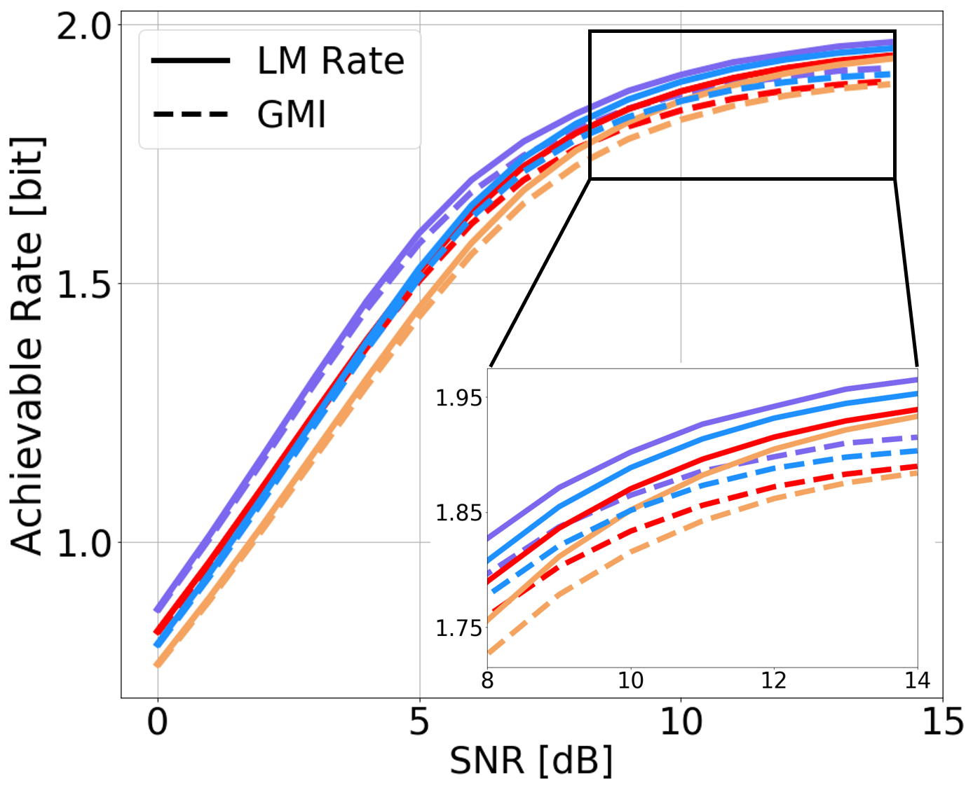
Figure 3: LM rate (solid) and GMI (dashed) versus SNR for the QPSK modulation scheme under different mismatched cases, including $(\eta,\theta)=(0.9,\pi/18)$ (Purple), $(\eta,\theta)=(0.8,\pi/18)$ (Blue), $(\eta,\theta)=(0.9,\pi/12)$ (Red), and $(\eta,\theta)=(0.8,\pi/12)$ (Orange).

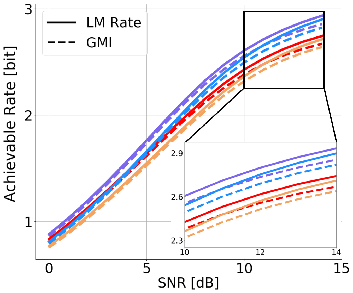
Figure 4: LM rate (solid) and GMI (dashed) versus SNR for the 16-QAM modulation scheme under different mismatched cases, including $(\eta,\theta)=(0.9,\pi/18)$ (Purple), $(\eta,\theta)=(0.8,\pi/18)$ (Blue), $(\eta,\theta)=(0.9,\pi/12)$ (Red), and $(\eta,\theta)=(0.8,\pi/12)$ (Orange).

In Fig. 3, we can see the comparison of the LM rate and GMI verse SNR for the QPSK modulation scheme. We observe that the LM rate is higher than GMI with the same parameters. Especially when $\text{SNR}>8$dB, there is about $2\%$ gain in the LM rate. In addition, as $\eta$ decreases (from $0.9$ to $0.8$) or $\theta$ increases (from $\pi/18$ to $\pi/12$), both LM rate and GMI decrease accordingly. These results agree with intuition. In Fig. 4, we display the comparison for the 16-QAM modulation scheme. From this, we can draw the same conclusions as those for Fig. 3.

V CONCLUSION

In this paper, we studied the computation problem of the LM rate, which is a lower bound for mismatch capacity. Our contributions are twofold. First, we showed that the computation of the LM rate can be reformulated into the Optimal Transport problem with an extra constraint. Second, we proposed a Sinkhorn-type algorithm to solve the above problem. For the extra constraint, we show that it is equivalent to seeking the root of a one-dimensional monotonic function. Numerical experiments show that our approach to computing the LM rate is efficient and accurate. Moreover, we can observe a noticeable gain in the LM rate compared to GMI.

References

- [1] N. Merhav, G. Kaplan, A. Lapidoth, and S. Shamai (Shitz), “On Information Rates for Mismatched Decoders,” IEEE Transactions on Information Theory, vol. 40, no. 6, pp. 1953–1967, Nov. 1994.
- [2] C. Shannon, “A Mathematical Theory of Communication,” The Bell System Technical Journal, vol. 27, no. 3, pp. 379–423,623–656, Jul.-Oct. 1948.
- [3] A. Lapidoth and S. Shamai (Shitz), “Fading Channels: How Perfect Need ‘Perfect Side Information’ Be?” IEEE Transactions on Information Theory, vol. 48, no. 5, pp. 1118–1134, May 2002.
- [4] W. Zhang, “A General Framework for Transmission with Transceiver Distortion and Some Applications,” IEEE Transactions on Communications, vol. 60, no. 2, pp. 384–399, Feb. 2012.
- [5] J. Salz and E. Zehavi, “Decoding under Integer Metrics Constraints,” IEEE Transactions on Communications, vol. 43, no. 2/3/4, pp. 307–317, Feb./Mar./Apr. 1995.
- [6] A. Lapidoth and P. Narayan, “Reliable Communication under Channel Uncertainty,” IEEE Transactions on Information Theory, vol. 44, no. 6, pp. 2148–2177, Oct. 1998.
- [7] J. Scarlett, A. Guillèn i Fábregas, A. Somekh-Baruch, and A. Martinez, “Information-Theoretic Foundations of Mismatched Decoding,” Foundations and Trends® in Communications and Information Theory, vol. 17, no. 2-3, pp. 149–400, 2020.
- [8] I. Csiszar and P. Narayan, “Channel Capacity for a Given Decoding Metric,” IEEE Transactions on Information Theory, vol. 41, no. 1, pp. 35–43, Jan. 1995.
- [9] G. Kaplan and S. Shamai (Shitz), “Information Rates and Error Exponents of Compound Channels with Application to Antipodal Signaling in a Fading Environment,” AEU-International Journal of Electronics and Communications, vol. 47, no. 4, pp. 228–239, Jul. 1993.
- [10] A. Asyhari and A. Guillèn i Fábregas, “Nearest Neighbor Decoding in MIMO Block-Fading Channels with Imperfect CSIR,” IEEE Transactions on Information Theory, vol. 58, no. 3, pp. 1483–1517, Mar. 2012.
- [11] A. Ganti, A. Lapidoth, and I. E. Telatar, “Mismatched Decoding Revisited: General Alphabets, Channels with Memory, and the Wide-Band Limit,” IEEE Transactions on Information Theory, vol. 46, no. 7, pp. 2315–2328, Nov. 2000.
- [12] R. H. Tütüncü, K. C. Toh, and M. J. Todd, “Solving Semidefinite-Quadratic-Linear Programs Using SDPT3,” Mathematical Programming, Series B, vol. 95, no. 2, pp. 189–217, 2003.
- [13] M. Grant and S. Boyd, “CVX Users’ Guide for CVX Version 1.21,” Jan. 2011.
- [14] M. Cuturi, “Sinkhorn Distances: Lightspeed Computation of Optimal Transport,” in Proc. Advances in Neural Information Processing Systems (NeurIPS), vol. 26, Lake Tahoe, Nevada, US, Dec. 2013, pp. 2292–2300.
- [15] G. Peyré and M. Cuturi, “Computational Optimal Transport: With Applications to Data Science,” Foundations and Trends® in Machine Learning, vol. 11, no. 5-6, pp. 355–607, Feb. 2019.
- [16] I. Csiszár and J. Körner, Information Theory: Coding Theorems for Discrete Memoryless Systems. Cambridge, UK: Cambridge University Press, 2011.
- [17] R. Sinkhorn, “Diagonal Equivalence to Matrices with Prescribed Row and Column Sums,” The American Mathematical Monthly, vol. 74, no. 4, pp. 402–405, Apr. 1967.