The Moment Passing Method for Wireless Channel Capacity Estimation

Abstract

Wireless network capacity can be regarded as the most important performance metric for wireless communication systems. With the fast development of wireless communication technology, future wireless systems will become more and more complicated. As a result, the channel gain matrix will become a large-dimensional random matrix, leading to an extremely high computational cost to obtain the capacity. In this paper, we propose a moment passing method (MPM) to realize the fast and accurate capacity estimation for future ultra-dense wireless systems. It can determine the capacity with quadratic complexity, which is optimal considering that the cost of a single matrix operation is not less than quadratic complexity. Moreover, it has high accuracy. The simulation results show that the estimation error of this method is below 2%. Finally, our method is highly general, as it is independent of the distributions of BSs and users, and the shape of network areas. More importantly, it can be applied not only to the conventional multi-user multiple input and multiple output (MU-MIMO) networks, but also to the capacity-centric networks designed for B5G/6G.

I Introduction

Wireless network capacity can be regarded as the most important performance metric for wireless communication systems. In 1948, a mathematical model to determine the channel capacity was first given by Dr. Claude E. Shannon[1]. He proposed that the capacity of a single input and single output channel can be determined according to the formula: $C=W\log(1+\frac{P}{N_{0}W})$ [2], where $W$ is the channel bandwidth, $P$ is the signal power and $N_{0}$ is the power of additive white Gaussian noise (AWGN). With the fast development of wireless technology, multiple antennas were equipped on both of the transmitter side and the receiver side, in order to improve the capacity. The uplink capacity of a multi-user multiple input and multiple output (MU-MIMO) network, which is equivalent to the capacity of a multiple access channel (MAC), can be determined according to [3] as:

$$C_{\mathrm{MAC}}\!=\!\mathbb{E}\{\log\det(\mathbf{I}\!+\!\frac{P}{N_{0}}\mathbf{H}\mathbf{H}^{*})\}\!=\!\mathbb{E}\sum_{j=1}^{t}\log(1\!+\!\frac{P}{N_{0}}\lambda_{j}),$$ (1)

where $\mathbf{H}\in\mathbb{C}^{t\times r}$ denotes the channel gain matrix, with $t$ and $r$ representing the number of transmit antennas and the number of receive antennas, respectively. $\mathbf{H}^{*}$ is the Hermitian conjugate of matrix $\mathbf{H}$. $\det(\cdot)$ represents the determinant of a matrix. $\lambda_{1},\cdots\lambda_{t}$ are the eigenvalues of the matrix $\mathbf{H}\mathbf{H}^{*}$.

It is well known that the computation of MAC capacity $C_{\mathrm{MAC}}$ is complicated. Specifically, $\mathbf{H}$ will become a large-dimensional random matrix as $t$ and $r$ increase. The matrix multiplication $\mathbf{H}\mathbf{H}^{*}$ consumes expensive time cost. The complexity of direct methods to compute $C_{\mathrm{MAC}}$, such as the Cholesky decomposition method (CDM) and the singular value decomposition (SVD) method, reaches $O(t^{3})$. This is unaffordable for future ultra-dense networks.

In 2021, a capacity-centric (C²) networking architecture designed for future ultra-dense wireless networks was proposed [4]. It can realize both high capacity and low signaling overhead simultaneously. The C² networking architecture is organized in the form of multiple non-overlapping clusters, with each cluster operating independently. Only base stations (BSs) belonging to the same cluster cooperate with each other, and the interference exists between different clusters, which can be called as the inter-cluster interference. Therefore, each cluster is equivalent to a MU-MIMO subnetwork, and a C² network can be regarded as a wireless network composed of multiple MU-MIMO subnetworks with interference between different subnetworks. For a C² network, the average capacity of the $m$-th cluster per BS is given in [4] as

$$C_{m}\!=\!\mathbb{E}\!\left\{\!\frac{1}{J_{m}}\!\log\det\left[\mathbf{I}\!+\!P(N_{0}\mathbf{I}\!+\!P\mathbf{\Pi}_{m}\mathbf{\Pi}_{m}^{*})^{-1}\mathbf{H}_{m}\mathbf{H}_{m}^{*}\right]\!\right\}\!,$$ (2)

where $\mathbf{H}_{m}$ and $\mathbf{\Pi}_{m}$ are the channel gain matrix and the interference matrix of cluster $m$ respectively, which will be specified later. With a little abuse of notation, we denote the term $P(N_{0}\mathbf{I}\!+\!P\mathbf{\Pi}_{m}\mathbf{\Pi}_{m}^{*})^{-1}\mathbf{H}_{m}\mathbf{H}_{m}^{*}$ as the signal to interference plus noise ratio (SINR) matrix. $J_{m}$ denotes the number of BSs. Obviously, (2) is much more complicated than (1) since (2) contains the inter-cluster interference. It is worth mentioning that in the special case where the number of clusters equals to one, all the BSs cooperate with each other, and no inter-cluster interference exists. The uplink channel of such a wireless network is equivalent to a MAC channel. That is, the formula (2) degenerates to (1). Therefore, without loss of generality, we will focus on the expression (2) and develop a fast and accurate numerical method to estimate $C_{m}$.

There are already some existing works to achieve the goal. In [4], the closed-form expressions of the upper and lower bounds of $C_{m}$ for uniformly distributed users scenario are derived. However, we don’t yet know how to generalize this to more general scenarios. Later, the TOSE algorithm [6] was proposed based on the random matrix theory (RMT) [7] for fast estimation of $C_{m}$, but it is less accurate.

In this paper, we propose a Moment Passing Method (MPM) to estimate the capacity of ultra-dense wireless networks. Inspired by the Marčenko-Pastur (MP) law in RMT, we propose a numerical approach to approximate the limiting spectral distribution (LSD) of the SINR matrix. By utilizing the characteristics of the random matrix, the high-complexity procedures including the matrix multiplication and the eigenvalue computation can be avoided. Therefore, our MPM is a low-complexity method. Different from the TOSE method [6], we directly estimate the LSD of the SINR matrix, avoiding an intermediate step of SINR matrix approximation in TOSE, and thus our MPM has higher accuracy. It should be further emphasized that the main novelty of our MPM is to combine the Stieltjes transform and the Laurent expansion to obtain the moment information of the LSD. This is the reason why we call this method Moment Passing Method (MPM). In the numerical simulations, we will show that the computational efficiency of MPM is almost identical to TOSE, but the numerical error is reduced by at least an order of magnitude compared with TOSE. In addition, MPM has superior generality since it is independent of the distributions of BSs and users, and the shapes of network areas. Finally, MPM is applicable not only to the conventional MU-MIMO networks, but also to the C² networks designed for B5G/6G.

II System Model

Consider a wireless network with $J$ single-antenna BSs $\mathcal{S}=\{s_{1},s_{2},\dots s_{J}\}$ and $K$ single-antenna users $\mathcal{U}=\{u_{1},u_{2},\dots,u_{K}\}$. The whole network is organized in the form of $M$ non-overlapping clusters $\mathcal{S}\bigcup\mathcal{U}=\bigcup_{m=1}^{M}\mathcal{C}_{m}$ [4]. Here, $\mathcal{C}_{m}$ represents the set of BSs and users belonging to the $m$-th cluster. The set of the BSs in $\mathcal{C}_{m}$ is denoted by $\mathcal{S}_{m}=\mathcal{S}\bigcap\mathcal{C}_{m}$, and similarly, the set of the users in $\mathcal{C}_{m}$ is $\mathcal{U}_{m}=\mathcal{U}\bigcap\mathcal{C}_{m}$. And we denote $J_{m}=|\mathcal{S}_{m}|$ and $K_{m}=|\mathcal{U}_{m}|$ the number of BSs and users in $\mathcal{C}_{m}$, respectively. To reflect the property of ultra-dense networks, we assume $J_{m}$ and $K_{m}$ approach infinity [4].

For the $m$-th cluster, we define the channel gain between the BS $s_{j}\in\mathcal{S}_{m}$ and the user $u_{k}\in\mathcal{U}$ as $h_{mjk}=l_{mjk}g_{mjk}$, where $g_{mjk}\sim\mathcal{CN}(0,1)$ is the small-scale fading and

$$l_{mjk}=\left\{\begin{array}[]{ll}d_{mjk}^{-1.75},&d_{mjk}>d_{1},\\ d_{1}^{-0.75}d_{mjk}^{-1},&d_{0}<d_{mjk}\leq d_{1},\\ d_{1}^{-0.75}d_{0}^{-1},&d_{mjk}\leq d_{0}\end{array}\right.$$ (3)

is the large-scale fading [4]. Here $d_{mjk}$ represents the Euclidean distance between the BS $s_{j}\in\mathcal{S}_{m}$ and the user $u_{k}$. The parameters $d_{0}$ and $d_{1}$ can be regarded as the near field threshold and far field threshold, respectively.

Thus, we can define the large-scale fading matrix $\mathbf{L}_{m}\in\mathbb{R}^{J_{m}\times K_{m}}$ and the small-scaling fading matrix $\mathbf{G}_{m}\in\mathbb{C}^{J_{m}\times K_{m}}$, with their $(j,k)$-th entry given by

$$[\mathbf{L}_{m}]_{jk}=l_{mjk},\quad[\mathbf{G}_{m}]_{jk}=g_{mjk}.$$

The channel gain matrix $\mathbf{H}_{m}$ in (2) can thus be defined as

$$\mathbf{H}_{m}=\mathbf{L}_{m}\circ\mathbf{G}_{m},$$ (4)

in which $\circ$ denotes the Hadamard product. The interference matrix $\mathbf{\Pi}_{m}$ can be similarly defined since it is also a Hadamard product between a large-scale fading matrix and a small-scale fading matrix. Details of deriving $\mathbf{\Pi}_{m}$ can be found in [8], and thus we do not repeat here due to space limitation. Define

$$\mathbf{\Xi}_{m}=N_{0}\mathbf{I}+P\mathbf{\Pi}_{m}\mathbf{\Pi}_{m}^{*},$$ (5)

as the noise-plus-interference matrix, with $\mathbf{\Xi}_{m}\in\mathbb{C}^{J_{m}\times J_{m}}$. It converges to a positive definite diagonal matrix as $J_{m}$ and $K-K_{m}$ approach infinity [8], which is

$$\mathbf{\Xi}_{m}=\textrm{diag}((N_{0}+P\xi_{11}^{m}),\dots,(N_{0}+P\xi_{J_{m}J_{m}}^{m})),$$ (6)

with $\xi_{jj}^{m}=\sum_{u_{k}\notin\mathcal{U}_{m}}l_{mjk}^{2}$. Substituting it into (2), we have

$$C_{m} =\mathbb{E}\left\{\frac{1}{J_{m}}\log\det\left(\mathbf{I}+P\mathbf{\Xi}_{m}^{-1/2}\mathbf{H}_{m}\mathbf{H}_{m}^{*}\mathbf{\Xi}_{m}^{-1/2}\right)\right\}$$

$$=\mathbb{E}\left\{\frac{1}{J_{m}}\log\det\left[\mathbf{I}+(\mathbf{Q}_{m}\circ\mathbf{G}_{m})(\mathbf{Q}_{m}\circ\mathbf{G}_{m})^{*}\right]\right\},$$ (7)

in which $\mathbf{Q}_{m}=P^{1/2}\mathbf{\Xi}_{m}^{-1/2}\mathbf{L}_{m}$.

In the following section, we will focus on (7) to develop the fast and accurate Moment Passing Method for the capacity estimation. As we have mentioned, $C_{\mathrm{MAC}}$ in (1) is a special case of $C_{m}$ (7). Therefore, the method developed in this paper is obviously applicable to (1).

III The Moment Passing Method

In this section, we will introduce our MPM to calculate the capacity based on (7). First, we transform the original problem of calculating matrix determinant (7) into the problem of computing the product of all matrix eigenvalues, as

$$C_{m}=\mathbb{E}\!\left[\frac{1}{J_{m}}\log\det(\mathbf{I}\!+\!\mathbf{A}_{m})\right]=\frac{1}{J_{m}}\mathbb{E}\sum_{j=1}^{J_{m}}\log(1\!+\!\lambda_{j}).$$ (8)

Here the SINR matrix $\mathbf{A}_{m}=\mathbf{B}_{m}\mathbf{B}_{m}^{*}\in\mathbb{C}^{J_{m}\times J_{m}}$ with $\mathbf{B}_{m}=\mathbf{Q}_{m}\circ\mathbf{G}_{m}$, and $\lambda_{j}\;(j=1,2,\cdots,J)$ gives all the eigenvalues of the SINR matrix $\mathbf{A}_{m}$. As we mentioned before, it is very expensive to solve all the eigenvalues of a large matrix, especially for $J_{m}\to\infty$. Moreover, we need to generate the SINR matrix $\mathbf{A}_{m}$ many times to obtain the expectation value in (8). Fortunately, based on RMT [9], we can approximate (8) using the following integral form

$$C_{m}\approx\int_{a}^{b}\log(1+x)f(x)\mathop{}\!\mathrm{d}x,$$ (9)

in which $f(x)$ is the LSD of $\mathbf{A}_{m}$. The lower and upper limits of the integral interval $[a,b]$ correspond to the minimum and maximum eigenvalues of the SINR matrix $\mathbf{A}_{m}$, respectively. Here, we introduce a hyper-parameter $\eta$, which can be understood as an approximation of the ratio between the minimum and maximum eigenvalues.

According to the MP-law in RMT [9], the LSD of the matrix $\widetilde{\mathbf{A}}_{m}=\mathbf{G}_{m}\mathbf{G}_{m}^{*}$, i.e. $\mathbf{Q}_{m}$ is an all-ones matrix, can be approximately written as

$$\widetilde{f}(x)\!=\!\frac{\beta}{2\pi K_{m}x}\sqrt{(b\!-\!x)(x\!-\!a)},\! \!\beta\!\geq\!1,$$ (10a)

$$\widetilde{f}(x)\!=\!(1\!-\!\beta)\delta(x)\!+\!\frac{\beta}{2\pi K_{m}x}\sqrt{(b\!-\!x)(x\!-\!a)},\! \!\beta\!<\!1.$$ (10b)

Note that the parameter $\beta=K_{m}/J_{m}$ in the above formulas represents the width-length ratio of the matrix $\mathbf{G}_{m}$. For $\beta<1$, the matrix $\widetilde{\mathbf{A}}_{m}$ is not full rank. Therefore, (10b) introduces the delta function $\delta(x)$ to characterize the distribution of zero eigenvalues.

For the LSD of the SINR matrix $\mathbf{A}_{m}$, there is currently no result in its analytic form. In this work, we hypothesize it can be approximated by a $N-$th order polynomial correction to the standard MP-law, i.e.

$$f(x)\!=\!\frac{\beta\!\sqrt{(b-x)(x-a)}}{2\pi K_{m}x}\sum_{k=0}^{N}\alpha_{k}x^{k}, \beta\!\geq\!1,$$ (11a)

$$f(x)\!=\!(1\!-\!\beta)\delta(x)\!+\!\frac{\beta\!\sqrt{(b-x)(x-a)}}{2\pi K_{m}x}\sum_{k=0}^{N}\alpha_{k}x^{k}, \beta\!<\!1.$$ (11b)

The rationality of the modification is that elements in $\mathbf{Q}_{m}$ are monotonically related to the distance between BSs and users in the network. And the difference between the elements in the matrix $\mathbf{Q}_{m}$ are limited. In the numerical experiments, we will show that the approximation to LSD gives a good estimation of capacity. As $N$ increases, the accuracy of capacity estimation is also improved. According to the numerical results, $N=3$ is good enough to estimate the capacity.

Next, we compute the polynomial coefficients $\alpha_{k}$ in (11) by using the moments

$$\phi_{j}=\int_{a}^{b}x^{j}f(x)\mathop{}\!\mathrm{d}x,\quad j=0,1,\cdots,N.$$ (12)

of the LSD of the SINR matix $\mathbf{A}_{m}$. By substituting (11) into (12), we have

$$\sum_{k=0}^{N}c_{j+k}\alpha_{k}=\phi_{j},\quad j=0,1,\cdots,N.$$ (13)

The parameters $c_{i}$ in the above formula can be pre-calculated as follows

$$c_{i}=\int_{a}^{b}x^{i}\frac{\beta\sqrt{(b-x)(x-a)}}{2\pi K_{m}x}\mathop{}\!\mathrm{d}x.$$

Finally, we need to get the moments $\phi_{j}$ of the LSD $f(x)$. They can be obtained by the Stieltjes transform [10] of the LSD $f(x)$, combined with the Laurent expansion [11]. This is the crucial point of our work, which we also illustrate with the following theorem. Since the information is transferred through the moments $\phi_{j}$, we name this method the Moment Passing Method (MPM).

Theorem 1

Consider the given matrix $\mathbf{Q}=[q_{ij}]\in\mathbb{R}^{p\times n}$ and the random matrix $\mathbf{G}\in\mathbb{C}^{p\times n}$, whose elements satisfy complex Gaussian distribution, the moments of the LSD $f(x)$ of the matrix $\mathbf{A}=(\mathbf{Q}\circ\mathbf{G})(\mathbf{Q}\circ\mathbf{G})^{*}$ are as follows:

$$\phi_{0}= 1,$$ (14)

$$\phi_{1}= \frac{1}{pn}\!\sum_{i=1}^{p}\sum_{k=1}^{n}\theta_{ik},$$ (15)

$$\phi_{2}= \frac{1}{pn^{2}}\!\sum_{i=1}^{p}\!\left[\!(\sum_{k=1}^{n}\theta_{ik})^{2}\!+\!\sum_{k=1}^{n}\theta_{ik}(\sum_{j=1}^{p}\theta_{jk})\!\right],$$ (16)

$$\phi_{3}= \frac{1}{pn^{3}}\!\sum_{i=1}^{p}\!\left[\!(\sum_{k=1}^{n}\theta_{ik})^{3}\!+\!2(\sum_{k=1}^{n}\theta_{ik})(\sum_{k=1}^{n}\theta_{ik}(\sum_{j=1}^{p}\theta_{jk}))\!\right]$$

$$+ \frac{1}{pn^{3}}\!\sum_{i=1}^{p}\sum_{k=1}^{n}\theta_{ik}\!\left[\!(\sum_{j=1}^{p}\theta_{jk})^{2}\!-\!(\sum_{j=1}^{p}\theta_{jk}(\sum_{l=1}^{n}\theta_{jl}))\!\right]\!,$$ (17)

with $\theta_{ij}=nq_{ij}^{2}$.

Proof:

According to [12], the Stieltjes transform of $f(x)$ satisfies

$$s(z) =\frac{1}{p}\sum_{i=1}^{p}\psi_{i},$$ (18)

$$\psi_{i}(z) =-\left[z(1+\frac{1}{n}\sum_{j=1}^{n}\theta_{ij}\tilde{\psi}_{j}(z))\right]^{-1},1\leq i\leq p,$$ (19)

$$\tilde{\psi}_{j}(z) =-\left[z(1+\frac{1}{n}\sum_{i=1}^{p}\theta_{ij}\psi_{i}(z))\right]^{-1},1\leq j\leq n.$$ (20)

When $|z|$ is larger than the maximum eigenvalue of $\mathbf{A}$, the Laurent expansion of $s(z)$ [9] is

$$s(z)=-\sum_{k=1}^{\infty}\frac{\phi_{k-1}}{z^{k}},$$ (21)

Define $u=1/z$, we have

$$s_{\mathbf{A}}(1/u)=-\phi_{0}u-\phi_{1}u^{2}-\phi_{2}u^{3}-\phi_{3}u^{4}+o(u^{4}).$$ (22)

Take the Taylor expansion of $\psi_{i}$ and $\tilde{\psi}_{j}$, we have

$$\psi_{i}=a_{i}u+b_{i}u^{2}+c_{i}u^{3}+d_{i}u^{4}+o(u^{4}),$$ (23)

$$\tilde{\psi}_{j}=\tilde{a}_{j}u+\tilde{b}_{j}u^{2}+\tilde{c}_{j}u^{3}+\tilde{d}_{j}u^{4}+o(u^{4}).$$ (24)

Plugging (23)-(24) into (19)-(20), we obtain

$$\begin{cases}a_{i}=&-1,\\ \tilde{a}_{j}=&-1,\\ b_{i}=&\frac{1}{n}\sum_{j=1}^{n}\theta_{ij}\tilde{a}_{j},\\ \tilde{b}_{j}=&\frac{1}{n}\sum_{i=1}^{p}\theta_{ij}a_{j},\\ c_{i}=&\frac{1}{n}\sum_{j=1}^{n}\theta_{ij}\tilde{b}_{j}-(\frac{1}{n}\sum_{j=1}^{n}\theta_{ij}\tilde{a}_{j})^{2},\\ \tilde{c}_{i}=&\frac{1}{n}\sum_{i=1}^{p}\theta_{ij}b_{i}-(\frac{1}{n}\sum_{i=1}^{p}\theta_{ij}a_{i})^{2},\\ d_{i}=&(\frac{1}{n}\sum_{j=1}^{n}\theta_{ij}\tilde{c}_{j})+(\frac{1}{n}\sum_{j=1}^{n}\theta_{ij}\tilde{a}_{j})^{3}\\ &-2(\frac{1}{n}\sum_{j=1}^{n}\theta_{ij}\tilde{a}_{j})(\frac{1}{n}\sum_{j=1}^{n}\theta_{ij}\tilde{b}_{j}),\\ \tilde{d}_{j}=&(\frac{1}{n}\sum_{i=1}^{p}\theta_{ij}c_{i})+(\frac{1}{n}\sum_{i=1}^{p}\theta_{ij}a_{i})^{3}\\ &-2(\frac{1}{n}\sum_{i=1}^{p}\theta_{ij}a_{i})(\frac{1}{n}\sum_{i=1}^{p}\theta_{ij}b_{i}),\end{cases}$$ (25)

Comparing it with (22), we can get the expressions of moments in (14)-(17). ∎

It should be emphasized that higher-order moments can also be obtained using the techniques above. However, the form of higher-order moments is too complicated, and we will not show them here. Based on the above discussions, we developed the Moment Passing Method, and the pseudo-code is presented in the following Algorithm.

Algorithm 1 The Moment Passing Method

0:  Distance $d_{mjk}$, hyper-parameter $\eta$

0:  Estimation of $C_{m}$.

1:  Calculate the matrix $\mathbf{L}_{m},\mathbf{\Xi}_{m}$ and $\mathbf{Q}_{m}$ with (3) and (6).

2:  Calculate the moments of LSD with (14)-(17).

3:  Generate $\mathbf{G}_{m}$, calculate $\mathbf{B}_{m}\!=\!\mathbf{Q}_{m}\circ\mathbf{G}_{m}$.

4:  Compute the maximum eigenvalue $b$ of $\mathbf{A}_{m}=\mathbf{B}_{m}\mathbf{B}_{m}^{*}$, and calculate $a=\eta b$.

5:  Use (9), (11) and (13) to compute $C_{m}$ with numerical integration.

Here, we use the power method to compute the maximum eigenvalue. In the iterative step, we can use $x^{(n+1)}=\mathbf{B}_{m}(\mathbf{B}_{m}^{*}x^{(n)})$ instead of $x^{(n+1)}=\mathbf{A}_{m}x^{(n)}$. This avoids the matrix multiplication operation $\mathbf{A}_{m}=\mathbf{B}_{m}\mathbf{B}_{m}^{*}$, and thus keeps the overall computational cost of $O(J_{m}^{2})$.

Another thing worth noting is that we do not directly calculate the minimum eigenvalue of the matrix. If the inverse power method is applied, it will result in the computational cost of $O(J_{m}^{3})$. In fact, we introduce a hyper-parameter $\eta$ to approximate the ratio between the minimum and maximum eigenvalues. According to the numerical simulations, the error of capacity estimation is not sensitive to the selection of hyper-parameter. Not only that, the computation of the non-zero minimum eigenvalue is extremely difficult for $\beta<1$. Therefore, we directly take $\eta=4\times 10^{-3}$ in the numerical simulation. This not only ensures numerical accuracy but also avoids excessively expensive computational costs.

IV Performance Evaluation

In this section, we demonstrate the high accuracy, efficiency, and generality of our MPM for the wireless capacity estimation through simulations.

Consider an ultra-dense network, where the network nodes (BSs and users) are deployed according to certain distributions. To reveal the generality of our MPM, we simulate two kinds of network areas: circle and square; and two kinds of network node distributions: uniform and normal. We use $D$ to denote the network diameter for the circle case, and the network side length for the square case. The whole network is decomposed into $M$ non-overlapping clusters based on the K-means algorithm [13], as illustrated in Fig. 1. We focused on the capacity of the cluster closest to the center of the entire network, which is highlighted in Fig. 1 by a black circle. The simulation results on capacity analysis for other clusters are similar, so we omit them due to space limitation. We also simulated the special case of C² in Fig. 2, where all the BSs cooperate and the number of clusters is one. This special case of C² is equivalent to a MU-MIMO network as discussed before.

To reduce the influence caused by randomness, we take the expectation value over 20 random experiments for each network scenario. Basic simulation parameters are listed in Table I. Unless otherwise specified, we take the ratio between the minimum and maximum eigenvalues $\eta$ as $4\times 10^{-3}$, and we use three moments for the computation, i.e., $N=3$ in (11). We perform $15$ iterations of the power method to compute the approximate maximum eigenvalue. All the experiments are conducted on a platform with an Intel(R) Core(TM) i5-12600KF CPU (10 cores) and 32G RAM.

TABLE I: The Network Setting

Definition and Symbol	Value
Network scale ($D$)	2000m
Near field threshold ($d_{0}$)	10m
Far field threshold ($d_{1}$)	50m
Power limit ($P$)	1W
Noise power ($N_{0}$)	$1\times 10^{-12}$ W
Number of clusters ($M$)	25

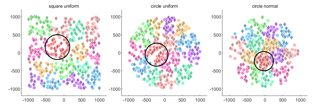
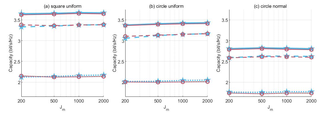
Figure 1: Top row: illustration of C² networks with three different settings. Different colors represent different clusters. Brighter dots represent BSs, and darker diamonds represent users. Bottom row: the capacity calculated by CDM (blue pentagram) and MPM (red circle). There are three different users-to-BSs ratios, which correspond to the dotted line $\beta=8$, the dashed line $\beta=2$, and the solid line $\beta=0.5$, respectively.

In Fig. 1 (top row), we present three different network scenarios.

• Square Uniform: uniformly distributed network nodes in the square network area (left column);

• Circle Uniform: uniformly distributed network nodes in the circle network area (middle column);

• Circle Normal: truncated normally distributed network nodes in the circle network area (right column);

In the bottom row of Fig. 1, we also present the capacity $C_{m}$ derived through two different methods (CDM and MPM), under different users-to-BSs ratios $\beta$, and different numbers of BSs $J_{m}$. Note that CDM computes $C_{m}$ according to the original capacity formula (7) directly, and thus can be considered as the baseline method. It can be observed from Fig. 1 that the capacity obtained by our MPM is almost the same as the baseline results. This demonstrates the high accuracy of our method. For the MU-MIMO systems in Fig. 2, similar results can be observed. Thus, we can draw the same conclusion that our MPM is with high accuracy on capacity estimation. In addition, Fig. 1-2 also demonstrate the generality of our MPM, since it has high accuracy under different network node distributions, different network shapes, and different values of $\beta$.

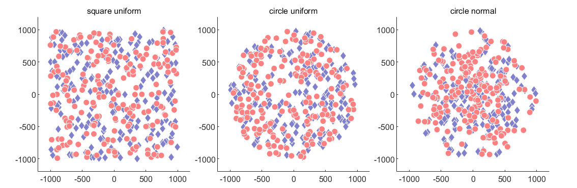
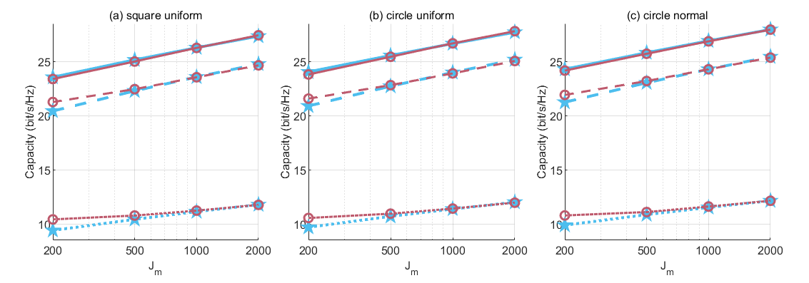
Figure 2: Top row: illustration of MU-MIMO networks, with three different settings. red dots represent BSs, and blue diamonds represent users. Bottom row: the capacity calculated by CDM (blue pentagram) and MPM (red circle). There are three different users-to-BSs ratios, which correspond to the dotted line $\beta=8$, the dashed line $\beta=2$, and the solid line $\beta=0.5$, respectively.

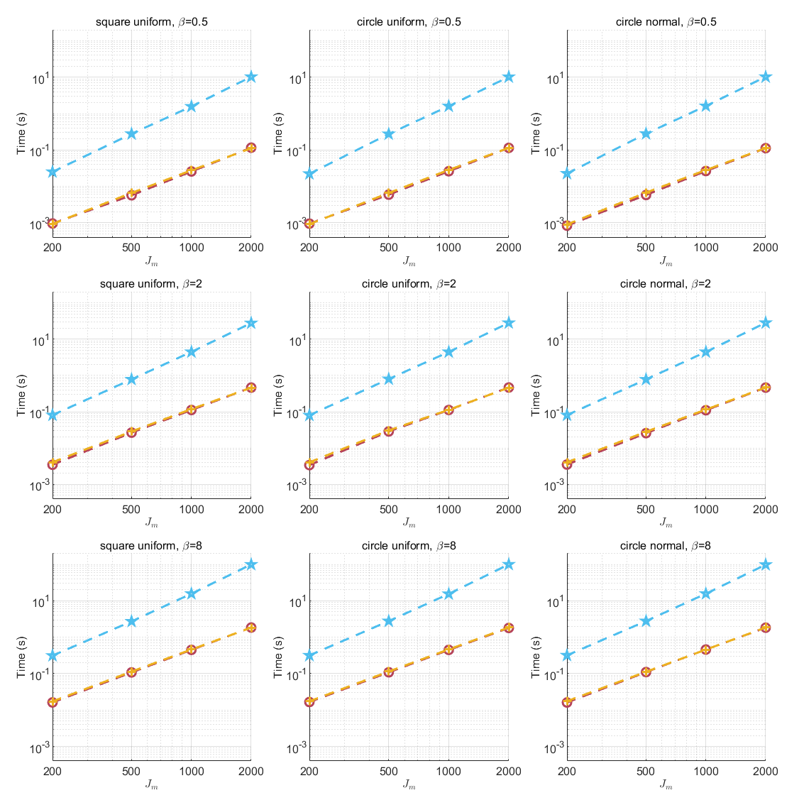
Figure 3: The comparison of computational time of MPM (red circle), TOSE (yellow plus sign) and CDM (blue pentagram). The top row ($\beta=0.5$), middle row ($\beta=2$) and bottom row ($\beta=8$) correspond to different users-to-BSs ratios $\beta$.

To study the efficiency advantage of our MPM, we present the computational time of three different methods in Fig. 3. By data fitting, we can see the empirical complexity of MPM, TOSE and CDM are $O(J_{m}^{2.05}),\;O(J_{m}^{2.06})$ and $O(J_{m}^{2.50})$ respectively. Combining the discussions of Fig. 1-2, we can see that although $C_{m}$ derived by MPM and CDM are almost the same, our MPM is much faster than CDM.

In Fig. 4, the relative errors of MPM and TOSE are output. Here we use CDM as the baseline for comparison. It can be seen that MPM is much more accurate than TOSE, although the computational time of MPM and TOSE are almost the same, as shown in Fig. 3. Thus, we can conclude that MPM is much better than TOSE for capacity estimation. In addition, in almost all numerical simulations, the relative error of MPM is less than $2\%$.

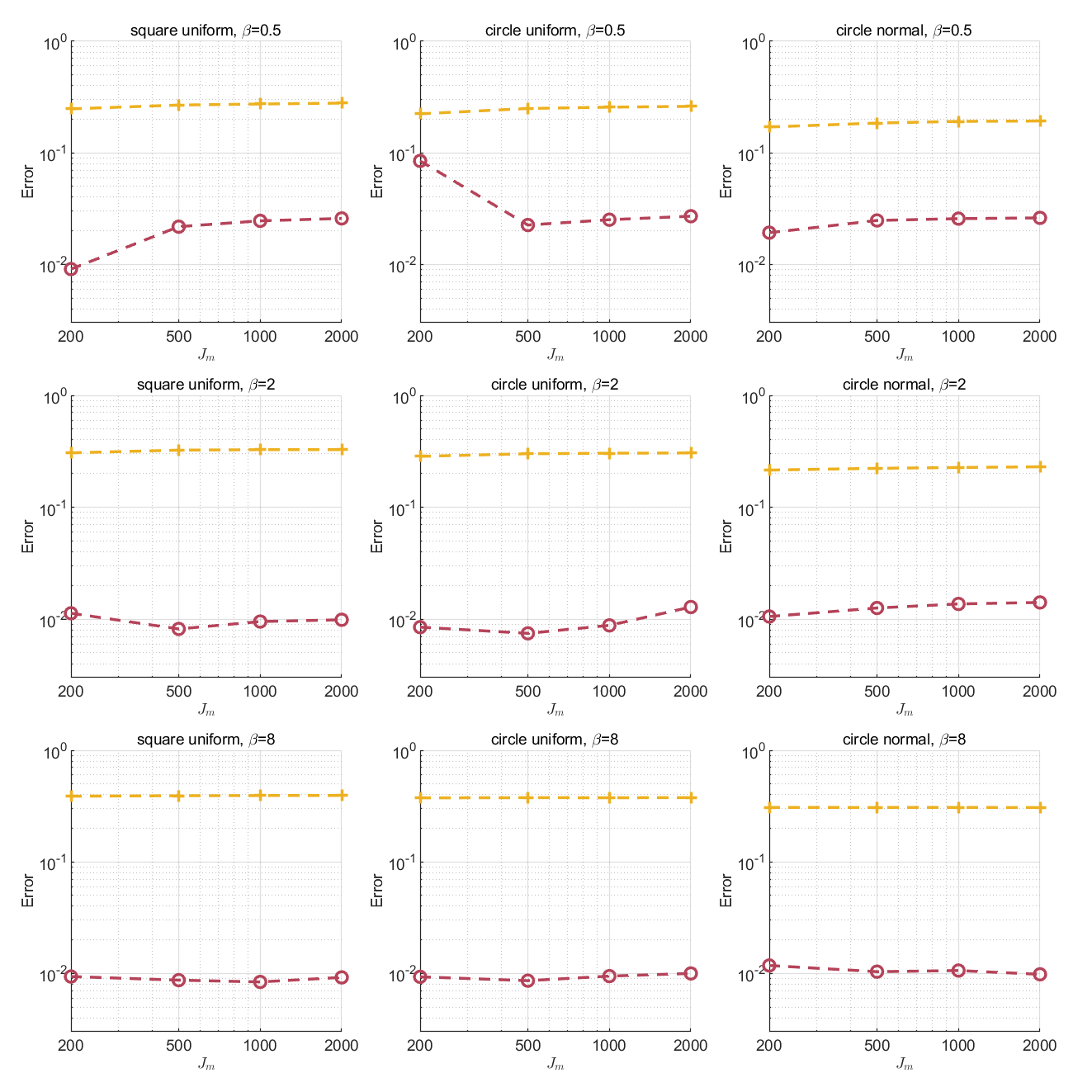
Figure 4: Comparisons of the capacity estimation error between MPM (red circle) and TOSE (yellow plus sign). The top row ($\beta=0.5$), middle row ($\beta=2$) and bottom row ($\beta=8$) correspond to different users-to-BSs ratios $\beta$.

In (11), we modify the original MP-law with an $N-$th order polynomial to approximate the LSD of the SINR matrix $\mathbf{A}_{m}$. Therefore, a natural question is whether we can obtain better accuracy for capacity as the polynomial order $N$ increases. In Fig. 5, the effect of different moments $N$ on the capacity are presented. The results are as we expected. The capacity computed by MPM keeps approaching that of CDM with the increase of $N=1,2,3$. However, the capacity estimation of four moments $N=4$ seems to be slightly worse than that of three moments. This may be due to Runge’s phenomenon of high order polynomial interpolation. Thus, $N=3$ of MPM could be a good choice for capacity estimation.

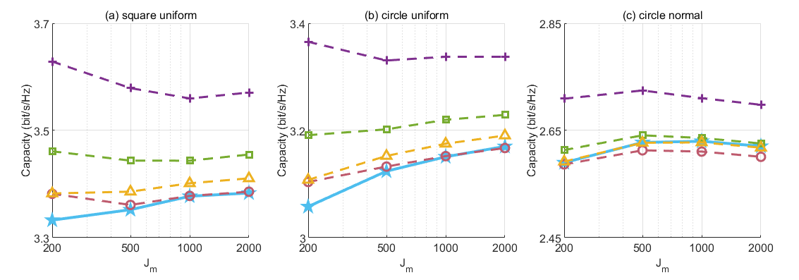
Figure 5: The comparison of MPM with different moments. The baseline is CDM (blue solid line with pentagram). The other four dashed lines show the capacity estimated by using the first one (purple plus sign), two (green square), three (red circle) and four (yellow triangle) moments.

Finally, we study the effect of hyper-parameter $\eta$ on the estimation capacity. As discussed at the end of Section 3, computing the non-zero minimum eigenvalue is very difficult and computationally expensive. Therefore, we approximate the maximum-minimum eigenvalue ratio by introducing the hyper-parameter $\eta$. After obtaining the maximum eigenvalue $b$, we can directly estimate the minimum eigenvalue $a=\eta b$. In Fig. 6, we present the capacity estimation results under different $\eta$. Meanwhile, the errors of capacity estimation with different $\eta$ are also presented in Tab. II. From the figure and table, we can see that the result of capacity estimation is not sensitive to $\eta$. Moreover, $\eta=4\times 10^{-3}$ seems to be an optimal choice.

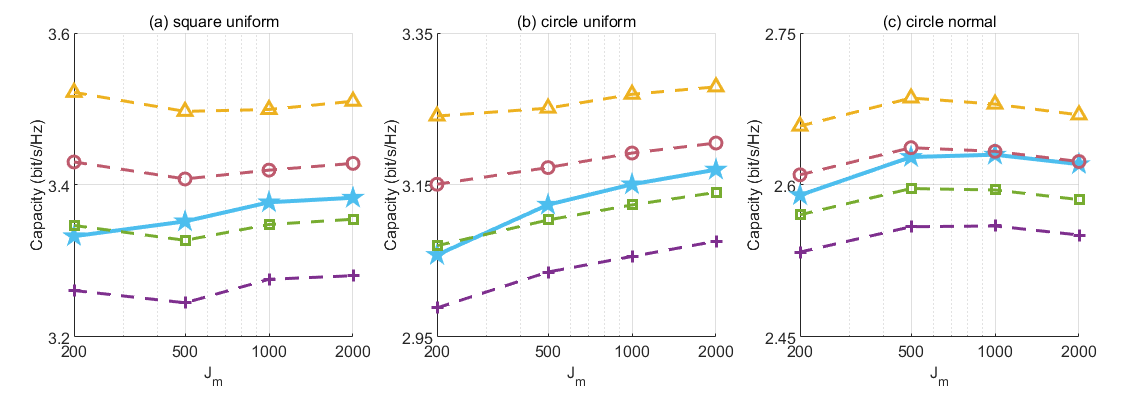
Figure 6: The comparison of MPM with different hyper-parameter $\eta$. The baseline is CDM (blue solid line with pentagram). The other four dashed lines show the capacity estimated with $\eta=0$ (purple plus sign), $\eta=10^{-3}$ (green square), $\eta=4\times 10^{-3}$ (red circle) and $\eta=10^{-2}$ (yellow triangle).

TABLE II: Capacity estimation errors of MPM with different hyper-parameter $\eta$ for circle uniform scenario.

	$\frac{1}{8}$	$\frac{1}{2}$	$2$	$8$	$32$
$0$	$2.12\%$	$4.91\%$	$2.92\%$	$1.46\%$	$1.23\%$
$0.5$	$1.76\%$	$3.35\%$	$1.54\%$	$1.09\%$	$1.02\%$
$1$	$1.62\%$	$2.72\%$	$1.00\%$	$0.94\%$	$0.93\%$
$2$	$1.44\%$	$1.85\%$	0.50%	$0.72\%$	$0.80\%$
$4$	$1.19\%$	0.68%	$1.28\%$	$0.42\%$	$0.60\%$
$8$	$0.85\%$	$0.94\%$	$2.88\%$	0.32%	$0.35\%$
$10$	$0.72\%$	$1.53\%$	$3.53\%$	$0.48\%$	0.28%
$20$	0.27%	$3.74\%$	$6.01\%$	$1.30\%$	$0.53\%$

V Conclusion

In this work, we propose the Moment Passing Method (MPM) to fast and accurately determine the capacity of ultra-dense and complicated networks. We can derive the moments of LSD of the SINR matrix with Stieltjes transform and Laurent expansion, which is not affected by different distributions of BSs and users and the shape of network areas. As such, we obtain the approximated LSD and the estimated capacity. Our MPM is feasible for both C² networks and conventional MU-MIMO networks, which shows great potential in the network design and analysis of the upcoming B5G/6G era.

It should be emphasized that the key of this work is the polynomial correction of the classical MP-law. Numerically, we can observe nice results for capacity estimation. It is worth studying the theoretical results of this correction, e.g., the convergence and the applicability to different problems. We are currently working on this and hope to report the progress in a future paper.

References

- [1] C. E. Shannon, “A mathematical theory of communication,” The Bell system technical journal, vol. 27, no. 3, pp. 379–423, 1948.
- [2] T. M. Cover and J. A. Thomas, Elements of Information Theory, 2nd ed. John Wiley & Sons, 2006.
- [3] D. Tse and P. Viswanath, Fundamentals of Wireless Communication. Cambridge University Press, 2005.
- [4] L. Yang, P. Li, M. Dong, B. Bai, D. Zaporozhets, X. Chen, W. Han, and B. Li, “C2: A capacity-centric architecture towards future wireless networking,” IEEE Trans. Wireless Commun., DOI: 10.1109/TWC.2022.3164286.
- [5] J. Wang, L. Dai, L. Yang, and B. Bai, “Clustered cell-free networking: a graph partitioning approach,” 2021, submitted to IEEE Trans. Wireless Commun. 2021.
- [6] D. Jiang, H. Han, L. Yang, and R. Wang, “TOSE: A fast capacity determination algorithm based on spike approximations,” submitted to IEEE VTC-FALL, 2022.
- [7] A. M. Tulino, S. Verdú. “Random matrix theory and wireless communications,” Foundations and Trends in Communications and Information Theory, vol. 1, no. 1, pp. 1–182, 2004.
- [8] C. Deng, L. Yang, H. Wu, D. Zaporozhets, M. Dong, and B. Bai, “CGN: A capacity-guaranteed network architecture for future ultra-dense wireless systems,” accepted by IEEE ICC 2022.
- [9] Z. Bai and J. W. Silverstein, Spectral analysis of large-dimensional random matrices. Springer, 2010, vol. 20.
- [10] H. S. Wall, Analytic theory of continued fractions. Van Nostrand, 1948.
- [11] W. Rudin, Real and Complex Analysis. McGraw-Hill, 1966.
- [12] W. Hachem, P. Loubaton, and J. Najim. “Deterministic equivalents for certain functionals of large random matrices,” The Annals of Applied Probability, vol. 17, no. 3, pp. 875–930, 2007.
- [13] S. P. Lloyd. “Least squares quantization in PCM,” IEEE Trans. Inf. Theory, vol. 28, no. 3, pp. 129–137, 1982.