Regression modelling of spatiotemporal extreme U.S. wildfires via partially-interpretable neural networks

Jordan Richards^1∗ and Raphaël Huser¹

March 13, 2024

Risk management in many environmental settings requires an understanding of the mechanisms that drive extreme events. Useful metrics for quantifying such risk are extreme quantiles of response variables conditioned on predictor variables that describe, e.g., climate, biosphere and environmental states. Typically these quantiles lie outside the range of observable data and so, for estimation, require specification of parametric extreme value models within a regression framework. Classical approaches in this context utilise linear or additive relationships between predictor and response variables and suffer in either their predictive capabilities or computational efficiency; moreover, their simplicity is unlikely to capture the truly complex structures that lead to the creation of extreme wildfires. In this paper, we propose a new methodological framework for performing extreme quantile regression using artificial neutral networks, which are able to capture complex non-linear relationships and scale well to high-dimensional data. The “black box" nature of neural networks means that they lack the desirable trait of interpretability often favoured by practitioners; thus, we unify linear, and additive, regression methodology with deep learning to create partially-interpretable neural networks that can be used for statistical inference but retain high prediction accuracy. To complement this methodology, we further propose a novel point process model for extreme values which overcomes the finite lower-endpoint problem associated with the generalised extreme value class of distributions. Efficacy of our unified framework is illustrated on U.S. wildfire data with a high-dimensional predictor set and we illustrate vast improvements in predictive performance over linear and spline-based regression techniques.

Keywords: deep learning; explainable AI; extreme quantile regression; neural networks; spatio-temporal extremes.

1 Introduction

1.1 Context and motivation

Uncontrolled wildfires are a significant cause of death and property damage across the world. Climate change is expected to increase both the severity and occurrence rate of wildfires with worrying trends predicted for the western United States (U.S.) (Smith et al., 2020), due to an increase in the frequency and intensity of extreme meteorological events: high temperatures, droughts and sufficiently fast windspeeds. Some of the most devastating wildfires in U.S. history have occurred most recently in California, with fires occurring between 2017 and 2020 being responsible for hundreds of deaths and an excess of one million acres of burnt land (Keeley and Syphard, 2021). Wildfires contribute to the accelerating rate of climate change through the emission of greenhouses gases; the year 2021 saw the release of an estimated 1760 megatonnes of carbon into the atmosphere as a direct consequence of wildfires (Copernicus, 2021), with a large proportion being attributed to wildfires in the northern U.S. Clearly the mitigation of risk and prevention of extreme wildfires, particularly events that lead to vast consumption of fuel, and hence, high carbon emissions, is of the utmost importance from both an economical and environmental perspective. In this paper, we develop new statistical methodology to quantify the effects of extreme wildfires through measures of burnt area, which are a useful proxy for both fuel consumption and emissions (Koh et al., 2021).

Estimation of extreme quantiles for spatio-temporal processes is important for risk management in a number of environmental applications, e.g., extreme precipitation (Huser and Davison, 2014; Opitz et al., 2018), heatwaves (Zhong et al., 2022), wind gusts (Castro-Camilo et al., 2019; Youngman, 2019). For processes observed over complex or large space-time domains, it is highly likely that the process will exhibit marginal non-stationarity, which can be handled by allowing the marginal distribution of the process to vary with both space and time. This can be achieved through a regression framework, i.e., with quantiles represented as functions of predictors. Let $\{Y(s,t):s\in\mathcal{S},t\in\mathcal{T}\}$ be a spatio-temporal process indexed by a spatial set $\mathcal{S}\subset\mathbb{R}^{2}$ and temporal domain $\mathcal{T}\subset\mathbb{R}_{+}$, and let $\{\mathbf{X}(s,t):s\in\mathcal{S},t\in\mathcal{T}\}$ denote a $d$-dimensional space-time process of predictor variables where $\mathbf{X}(s,t)=(X_{1}(s,t),\dots,X_{d}(s,t))$ for all $(s,t)\in\mathcal{S}\times\mathcal{T}$ and for $d\in\mathbb{N}$. We denote observations of $\mathbf{X}(s,t)$ by $\mathbf{x}({s,t})\in\mathbb{R}^{d}$ and note that the process need not be smooth spatially, nor temporally. Our interest lies in the upper-tail behaviour of $Y(s,t)\mid\{\mathbf{X}(s,t)=\mathbf{x}({s,t}):(s,t)\in\mathcal{S}\times\mathcal{T}\}$, which can be characterised through its quantile function; this can be estimated either non-parametrically or parametrically, with the latter approach typically relying on parametric extreme value distributions (see, e.g., Chavez-Demoulin and Davison (2005)). Although non-parametric approaches avoid making restrictive assumptions about the behaviour of $Y(s,t)$, they cannot reliably be used to make inference beyond the range of observations, i.e., estimation of quantiles larger than those previously observed; to that end, we turn to asymptotically-justified extreme value models. We unify here quantile regression and extreme value theory to provide more accurate estimation of the tails of $Y(s,t)$.

1.2 Classical extreme-value modelling

Coles (2001) details three main approaches to modelling univariate extreme values of a sequence of independent random variables $Y_{1},\dots,Y_{n}$ with common distribution function $F$; see also the review by Davison and Huser (2015). The first concerns block-maxima $M_{n}=\max\{Y_{1},\dots,Y_{n}\}$; if there exists sequences $\{a_{n}>0\}$ and $\{b_{n}\}$ such that

$${\rm Pr}\{(M_{n}-b_{n})/a_{n}\leq z\}\rightarrow G(z)\;\;\text{as}\;\;n\rightarrow\infty,$$ (1)

for non-degenerate $G$, then $F$ is in the max-domain of attraction (MDA) of $G$, the generalised extreme value GEV$(\mu,\sigma,\xi)$ distribution function, where

$$G(z\mid\mu,\sigma,\xi)=\begin{cases}\exp\left[-\left\{1+\xi\left({\textstyle{z-\mu\over\sigma}}\right)\right\}_{+}^{-1/\xi}\right],\;\;&\xi\neq 0,\\ \exp\left\{-\exp\left(-{\textstyle{z-\mu\over\sigma}}\right)\right\},\;\;&\xi=0,\end{cases}$$ (2)

with $\{y\}_{+}=\max\{0,y\}$, location, scale, and shape, parameters $\mu\in\mathbb{R},\sigma>0$, and $\xi\in\mathbb{R}$, respectively, and support $\{z\in\mathbb{R}:1+\xi(z-\mu)/\sigma>0\}$. Another approach, the so-called peaks-over-threshold method, utilises the generalised Pareto distribution (GPD), which can be used to model exceedances of $Y$ above some high threshold $u$. Given that $F$ is in the MDA of a GEV$(\mu,\sigma,\xi)$ distribution, then $(Y-u)\mid Y>u$ can be approximated by a GPD$(\sigma_{u},\xi)$ random variable with distribution function $H(z)=(1+\xi z/\sigma_{u})^{-1/\xi}$ and support $z\geq 0$ for $\xi\geq 0$ and $0\leq z\leq-\sigma_{u}/\xi$ for $\xi<0$, and where $\sigma_{u}=\sigma+\xi(u-\mu)>0$. For both the GEV and GPD, the shape $\xi$ controls the lower and upper bounds of $H$ and $G$. If $\xi<0$, then $H$ and $G$ are bounded above; for $\xi>0$, then $G$ is bounded below. Modelling with distributions that have finite bounds dependent on model parameters can lead to unstable inference (Smith, 1985), and so we constrain $\xi>0$ throughout; the assumption that wildfire burnt areas are heavy-tailed has been shown to hold in a number of studies (see references in Pereira and Turkman (2019)). Castro-Camilo et al. (2022) overcome the finite lower-bound problem for $G$ when $\xi>0$, which we discuss and extend in Section 3.2. To capture non-stationarity, we assert that the GEV and GPD parameters can be represented as functions of $\mathbf{X}(s,t)$, and denote these distributions by GEV$(\mu(s,t),\sigma(s,t),\xi(s,t))$ and GPD$(\sigma_{u}(s,t),\xi(s,t))$, respectively, where $\sigma_{u}(s,t)$ is dependent on a spatio-temporal threshold $u(s,t)$.

Use of the GEV and GPD distributions for spatio-temporal regression is not practical in all applications. The GEV distribution is applicable to block-maxima and so transformation of covariates may be necessary to make modelling feasible, e.g., aggregating blocks of predictors. Whilst the GPD does not suffer from this issue, it requires two separate models for full inference on the distribution of $Y(s,t)$, i.e., models for $Y(s,t)\mid Y(s,t)>u(s,t)$ and ${\rm Pr}\{Y(s,t)>u(s,t)\}$; moreover, the scale parameter $\sigma_{u}(s,t)$ is dependent on the threshold $u(s,t)$, which makes interpretation of its drivers difficult. Smith (1989) details a third method for modelling extremes using point processes (PP), which circumvents the issues associated with the GEV and GPD models. Assume limit (1) holds and $G$ has lower- and upper-endpoints $z_{-}$ and $z_{+}$, respectively. Then for any $u>z_{-}$, the sequence of point processes $N_{n}=\{(i/(n+1),(Y_{i}-b_{n})/a_{n}):i=1,\dots,n\}$ converges on regions $(0,1)\times(u,\infty)$ as $n\rightarrow\infty$ to a Poisson point process with intensity measure $\Lambda$ of the form $\Lambda(A)=-(t_{2}-t_{1})\log G(z)$, where $A=[t_{1},t_{2}]\times[z,z_{+})$ for $0\leq t_{1}\leq t_{2}\leq 1$; with an abuse of notation, we write $Y\sim\mbox{PP}(\mu,\sigma,\xi;u)$ if $Y$ satisfies the limiting Poisson process conditions. Details for modelling using this approach and an extension thereof are given in Section 3.

1.3 Extreme-value regression framework

Throughout we assume that extremes of $Y(s,t)\mid\{\mathbf{X}(s,t)=\mathbf{x}({s,t}):(s,t)\in\mathcal{S}\times\mathcal{T}\}$ can be modelled through an approach using a generic extreme value distribution EV with parameter set $\{\boldsymbol{\theta}(s,t):s\in\mathcal{S},t\in\mathcal{T}\}$ which is dependent on the predictors, i.e., for all $i=1,\dots,p$ for $p=|\boldsymbol{\theta}(s,t)|$, we have $\theta_{i}(s,t)=m_{i}(\mathbf{x}(s,t))$ for functions $m_{i}:\mathbb{R}^{d}\rightarrow\mathbb{R}$. Thus our proposed framework is flexible; we consider an arbitrary modelling approach with parametric model EV. For example, in the case of the peaks-over-threshold framework, our approach would be to model extreme values of $Y(s,t)\mid\{\mathbf{X}(s,t)\}$ by assuming that $(Y(s,t)-u(s,t))\mid\{\mathbf{X}(s,t)\}\sim\mbox{GPD}(\sigma_{u},\xi)$; here EV$\sim$GPD and $\boldsymbol{\theta}(s,t)=(\sigma_{u}(s,t),\xi(s,t))$. For the cases where EV$\sim$GEV and EV$\sim$PP, the distributions are parametrised by $\boldsymbol{\theta}(s,t)=(\mu(s,t),\sigma(s,t),\xi(s,t))$.

Extreme value regression using linear functions for $m_{i}$ has been exploited in a number of spatial studies (Mannshardt-Shamseldin et al., 2010; Davison et al., 2012; Eastoe, 2019). However, such models are incapable of capturing complex, non-linear relationships between the predictors and the response. Bayesian hierarchical modelling can be used to capture behaviour not explainable by linear models by assuming that the marginal parameters come from a latent process (Casson and Coles, 1999; Cooley et al., 2007; Sang and Gelfand, 2010; Opitz et al., 2018; Hrafnkelsson et al., 2021); these methods often require parametric assumptions for inference and scale poorly for large $d$ or for many observations. Semi-parametric regression has also been considered for spatial extremes modelling, where distribution parameters are represented as smooth, additive functions of predictors using splines or piece-wise linear functions (Chavez-Demoulin and Davison, 2005; Jonathan et al., 2014; Youngman, 2019; Zanini et al., 2020). For example, Youngman (2019) estimate extreme spatio-temporal quantiles by representing the parameters of the GPD and exceedance threshold using generalised additive models (GAMs). Whilst semi-parametric approaches provide a much more flexible class of models compared to linear models, they can be computationally expensive to fit, particularly if $d$ or $|\mathcal{S}\times\mathcal{T}|$ are large.

1.4 Machine learning for extreme-value analysis

Recent literature has seen the development of machine learning approaches for extreme value analyses. These algorithms often lack interpretability, but can be used to produce accurate and computationally fast predictions of extreme values for high-dimensional datasets; moreover, they are capable of capturing much more complex structures in data than linear models or GAMs. Such approaches applied in a regression context include the fitting of GPD models with trees (Farkas et al., 2021), random forests (Gnecco et al., 2022) and gradient boosting (Velthoen et al., 2021). Other machine learning algorithms have also been adapted for modelling extreme values, e.g., anomaly detection and classification (Clifton et al., 2014; Rudd et al., 2017; Vignotto and Engelke, 2020), sparse learning (see review by Engelke and Ivanovs (2021)), principal component analysis (Cooley and Thibaud, 2019; Drees and Sabourin, 2021), and clustering (Chautru, 2015; Janßen and Wan, 2020).

A somewhat untapped class of tools for modelling spatio-temporal extreme values are deep learning methods or neural networks (NNs). In the extreme value literature, Cannon (2018) perform multiple-level extreme quantile regression for precipitation using a monotone quantile regression network. Cannon (2010, 2011), Vasiliades et al. (2015), Bennett et al. (2015) and Shrestha et al. (2017) use NNs to estimate GEV parameters and Rietsch et al. (2013) apply a similar approach to fit GPD models; we refer to neural networks that are specifically used to fit parametric regression models, e.g., our EV model, as conditional density estimation networks (CDNs). Carreau and Bengio (2007) and Carreau and Vrac (2011) use CDNs to fit mixture models, with the upper-tails characterised using the GPD. A spatial extremes analysis is conducted by Ceresetti et al. (2012), who produce spatial maps of precipitation return levels by estimating non-stationary GEV and GPD parameters using a simple one-layer feed-foward network; this, and the above methods, all utilise multi-layered perceptron (MLP) neural networks. Here we use MLP to describe the class of feed-forward neural networks where all layers are densely-connected (see Appendix A.3.2) and which are not particularly well suited for identifying spatial or temporal structures within predictors; hence we consider more complex networks better suited to modelling spatio-temporal data. A comprehensive review of MLPs and their extensions, to be discussed, is given by Ketkar and Santana (2017). In the context of extreme value analysis, extensions of MLPs are utilised by Allouche et al. (2021), who construct a generative adversial network (GAN) for estimating quantiles of heavy-tailed distributions, and Boulaguiem et al. (2022), who use a GAN for modelling extreme spatial dependence and performing stochastic weather generation.

For spatial problems, a better alternative to an MLP are those that include layers with convolutional filters, often referred to as convolutional NNs (CNNs) (see the reviews by Yamashita et al. (2018) and Gallego and Ríos Insua (2022)). CNNs were first advocated for image classification due to their ability to capture spatial structures within images; Medina et al. (2017) and Driss et al. (2017) find that CNNs perform much better than MLPs for spatial classification problems. CNNs have been used in a number of environmental applications: classification (Gebrehiwot et al., 2019; Zhang et al., 2019), regression (Rodrigues and Pereira, 2020; Yu et al., 2020), and downscaling (Harilal et al., 2021). Lenzi et al. (2021) use CNNs to fit max-stable processes for modelling extreme spatial dependence.

To learn temporal structures in $\mathbf{X}(s,t)$, we can use recurrent layers, which have been shown to give improved forecasting of time series when compared to MLPs (Barbounis et al., 2006; Biancofiore et al., 2015). Long short-term memory (LSTM) layers are a popular type of recurrent layer (Hochreiter and Schmidhuber, 1997) and have been successfully used for prediction in a number of environmental applications, e.g., North Atlantic Oscillation index (Yuan et al., 2019), influenza trends (Liu et al., 2018b), sea surface temperatures (Liu et al., 2018a) and basin water levels (Shuofeng et al., 2021). LSTM layers can be combined with convolutional layers to create a network that can capture both spatial and temporal characteristics of data; we denote networks that use only convolutional LSTM layers as CNN-LSTM NNs, and those that use only dense LSTM layers as MLP-LSTM NNs.

1.5 Towards interpretable deep learning for extremes

A potential drawback of using NNs for modelling is their lack of interpretability, which is a desirable trait for methods used to perform statistical inference, as they often contain a large number of parameters; a trait shared with many other machine learning approaches. Recent work has been done on interpreting the outputs of machine learning algorithms, see, e.g., Bau et al. (2017); Zhang and Zhu (2018); Samek et al. (2021), but not in the context of performing regression. However, Zhong and Wang (2021) propose a framework for non-parametric quantile regression using neural networks which are partially linear, with the linear part of the model considered to be interpretable. For a univariate response variable $Y$, they represent its quantile at a pre-specified level by $\mathbf{x}^{T}\boldsymbol{\eta}+m(\mathbf{z})+\epsilon$, where $(\mathbf{x},\mathbf{z})\in\mathbb{R}^{l}\times\mathbb{R}^{d-l}$ are covariates, $\boldsymbol{\eta}\in\mathbb{R}^{l}$ is a set of parameters and $m:\mathbb{R}^{d-l}\rightarrow\mathbb{R}$ is an unknown function, with heteroscedastic errors $\epsilon$. Here $\mathbf{x}$ and $\mathbf{z}$ are both covariates that affect the distribution of $Y$, but only the contribution from $\mathbf{x}$ is of interest. Inference on the effect of $\mathbf{x}$ on $Y$ is conducted by considering the estimated values of the regression coefficients $\boldsymbol{\eta}$, whilst the covariates $\mathbf{z}$ feed an MLP which is used to estimate the unknown function $m$; inference on $m$ is not necessary as their interest lies in the effect of $\mathbf{x}$ on $Y$ only. Hence, their approach balances interpretability with the high predictive accuracy of deep learning methods. In this paper, we extend their approach by using a partially linear model for the parameters of the EV distribution and consider different network architectures to estimate $m$. To gain in flexibility, we further incorporate an additional interpretable component alongside the linear one, which is modelled using splines.

Recall that we consider $\mbox{EV}(\boldsymbol{\theta}(s,t))$ where $\boldsymbol{\theta}(s,t)=(\theta_{1}(s,t),\dots,\theta_{p}(s,t))$. For each $\theta_{i}(s,t)$ and for all space-time locations $(s,t)\in\mathcal{S}\times\mathcal{T}$, we divide the predictor process $\mathbf{X}(s,t)$ into three complementary components. For $l_{i},a_{i}\in\mathbb{N}$ and $l_{i}+a_{i}\leq d$, let $\mathbf{X}^{(i)}_{\mathcal{L}}(s,t)\in\mathbb{R}^{l_{i}},\mathbf{X}^{(i)}_{\mathcal{A}}(s,t)\in\mathbb{R}^{a_{i}}$ and $\mathbf{X}^{(i)}_{\mathcal{N}}(s,t)\in\mathbb{R}^{d-l_{i}-a_{i}}$ be distinct sub-vectors of $\mathbf{X}(s,t)$, with observations of each component denoted $\mathbf{x}^{(i)}_{\mathcal{L}}(s,t),\mathbf{x}^{(i)}_{\mathcal{A}}(s,t)$ and $\mathbf{x}^{(i)}_{\mathcal{N}}(s,t)$, respectively. Note that the indices mapping $\mathbf{x}(s,t)$ to $\mathbf{x}^{(i)}_{\mathcal{L}}(s,t)$ are consistent for all $(s,t)$, and similarly for $\mathbf{x}^{(i)}_{\mathcal{A}}(s,t)$ and $\mathbf{x}^{(i)}_{\mathcal{N}}(s,t)$; however, they need not be consistent across each $i=1,\dots,p$. For all $i=1,\dots,p$, each parameter $\theta_{i}(s,t)$ is then represented through the unified model

$$\theta_{i}(s,t)=h_{i}[\eta^{(i)}_{0}+m^{(i)}_{\mathcal{L}}\{\mathbf{x}^{(i)}_{\mathcal{L}}(s,t)\}+ m^{(i)}_{\mathcal{A}}\{\mathbf{x}^{(i)}_{\mathcal{A}}(s,t)\}+m^{(i)}_{\mathcal{N}}\{\mathbf{x}^{(i)}_{\mathcal{N}}(s,t)\}]$$ (3)

for constant intercept $\eta^{(i)}_{0}\in\mathbb{R}$, a linear function $m^{(i)}_{\mathcal{L}}(\mathbf{x})=\mathbf{x}^{T}\boldsymbol{\eta}^{(i)}$ for $\boldsymbol{\eta}^{(i)}\in\mathbb{R}^{l_{i}}$ and (potentially) non-linear functions $m^{(i)}_{\mathcal{A}}:\mathbb{R}^{a_{i}}\rightarrow\mathbb{R},m^{(i)}_{\mathcal{N}}:\mathbb{R}^{d-l_{i}-a_{i}}\rightarrow\mathbb{R}$, and $h_{i}:\mathbb{R}\rightarrow\mathbb{R}$; note that the range of $\theta_{i}(s,t)$ is controlled by the link function $h_{i}$. The function $m^{(i)}_{\mathcal{A}}$ is here modelled using splines, while $m^{(i)}_{\mathcal{N}}$ is approximated via a neural network with a suitable architecture. Thus, we choose $\mathbf{x}^{(i)}_{\mathcal{L}}(s,t)$ and $\mathbf{x}^{(i)}_{\mathcal{A}}(s,t)$ as those predictors for which we wish to infer their relationship on $Y(s,t)$; all other predictors go into $\mathbf{x}^{(i)}_{\mathcal{N}}(s,t)$. A heuristic for deciding which interpretable predictors are modelled using the linear or additive functions is given in Section 4.1. We denote models that utilise the full unified representation (3) by “lin+GAM+NN" models, and similarly for sub-classes. In the cases where $m_{\mathcal{A}}(s,t)=m_{\mathcal{N}}(s,t)=0$ for all $(s,t)$, we denote the model “fully-linear"; similar nomenclature is used for “fully-GAM" and “fully-NN" models. The strength and novelty of our proposed framework is that it unifies, for the first time, the theoretical guarantees of parametric EV models, the interpretability of generalised additive models, and the predictive power of artificial neural networks in a single model. Whilst our focus is on estimating the distribution EV, it is trivial to see how the lin+GAM+NN framework can be adapted to estimate other parametric statistical distributions, as well as perform more classical applications of NNs, e.g., classification and mean, median, or quantile, regression; we perform logistic, and single-level non-parametric quantile, regression using a GAM+NN model in Section 4.

The rest of the paper is outlined as follows. Section 2 describes the data used in our analyses and the scientific questions we address. In Appendices A.2 and A.3, we describe the additive functions and neural networks used to model $m_{\mathcal{A}}$ and $m_{\mathcal{N}}$, respectively. The use of neural networks in our unified framework creates new challenges for fitting extreme value models where distributional lower bounds are dependent on model parameters; a discussion of these issues is provided in Appendix A.3.5, with details of a new approach for modelling extreme values using point processes that solves these problems given in Section 3. To illustrate the efficacy of our modelling framework, we apply our approach to simulated data in Appendix B (with a summary provided in Section 3.3) and U.S. wildfires data in Section 4; many different candidate models are proposed and their individual predictive performances is assessed.

2 Wildfire data

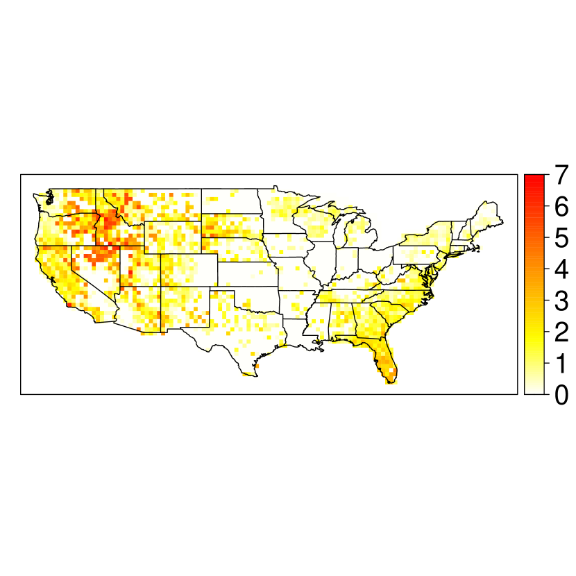
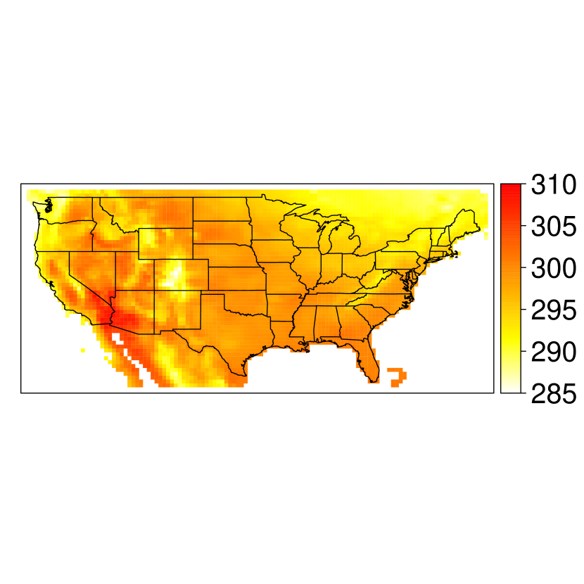
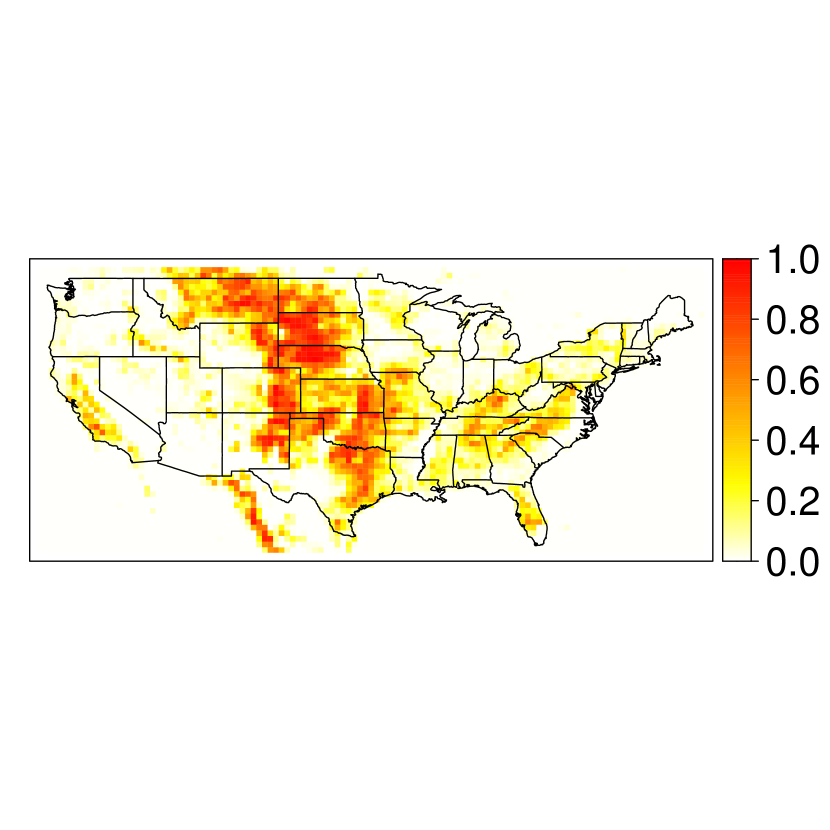
Figure 1: Maps of (left) observed $\log(1+\sqrt{Y}(s,t))$, (centre) temperature and (right) proportion of grassland coverage for July, 2007.

The response data we use in our analyses are observations of monthly aggregated burnt area (acres) of 3503 spatial grid-cells located across the contiguous United States; the spatial domain $\mathcal{S}$ is illustrated in Figure 1. The observation period covers 1993 to 2015, using only months between March and September, inclusive, leaving 161 observed spatial fields. Grid-cells are arranged on a regular latitude/longitude grid with spatial resolution $0.5^{\circ}\times 0.5^{\circ}$. Observations are provided by the Fire Program Analysis fire-occurrence database (Short, 2017) which collates U.S. wildfire records from the reporting systems of federal, state and local organisations. A subset of these data are described by Opitz (2022) and have been previously studied as part of a data prediction challenge for the Extreme Value Analysis (EVA) 2021 conference, see, e.g., Cisneros et al. (2021), D’Arcy et al. (2021), Koh (2021) and Zhang et al. (2022), with Ivek and Vlah (2022) using deep learning methods. Whilst the focus of this challenge was on predicting extreme quantiles for missing spatio-temporal locations, our focus is instead on inference of relationships between predictors and extreme quantiles of burnt area; hence, we utilise all of the available data for modelling.

We have $d=30$ predictors of three classes: orographical, land coverage and meteorological. The two orographical predictors are the mean and standard deviation of the altitude for each grid-cell; estimates are derived using a densely-sampled gridded output from the U.S. Geographical Survey Elevation Point Query Service. The standard deviation of the altitude is here used as a proxy for terrain roughness. The land cover variables that are considered describe the proportion of a grid-cell which is covered by one of 18 different types, e.g., urban, grassland (illustrated in Figure 1), water (see Opitz (2022) for full details). Land cover predictors are derived using a gridded land cover map, of spatial resolution $300$m and temporal resolution one year, produced by COPERNICUS and available through their Climate Data Service. For each $0.5^{\circ}\times 0.5^{\circ}$ grid-cell, the proportion of a cell consisting of a specific land cover type is derived from the high-resolution product. Ten meteorological variables are considered and given as monthly means. These variables are provided by the ERA5-reanalysis on land surface, also available through the COPERNICUS Climate Data Service, which is given on a $0.1^{\circ}\times 0.1^{\circ}$ grid; the values are then aggregated to a $0.5^{\circ}\times 0.5^{\circ}$ resolution. The variables are: both eastern and northern components of wind velocity at a 10m altitude, both dew-point temperature and temperature at a 2m altitude (see Figure 1), potential evaporation, evaporation, precipitation, surface pressure and surface net solar, and thermal, radiation. This particular ERA5-reanalysis samples over land only, and so the meteorological conditions over the Pacific and Atlantic oceans are not available for our analyses; further discussion of this problem is provided in Section 4.1. Note that, for us to utilise CNN and recurrent layers in our model, the spatio-temporal domain over which predictors are observed is slightly larger than that associated with the response, see Figure 1.

In Section 4.3, we focus on quantifying the drivers of wildfire occurrence and the extremal behaviour of wildfire spread, particularly if those drivers are meteorological variables that will see their own extremal behaviour exasperated by climate change. We use our proposed methodology to produce maps of monthly occurrence risk and extreme quantiles for wildfire spread; the former can be used to identify areas of high susceptibility to wildfire occurrence, whilst the latter illustrates locations where it is of particular pertinence to prevent wildfires.

3 Extreme point process model

3.1 Modelling extremes with point processes

To model non-stationary extreme values with the PP approach, we first assume that limit $\eqref{max_lim}$ holds at each space-time location $(s,t)\in\mathcal{S}\times\mathcal{T}$. That is, for multiple realisations $Y_{i}(s,t)$ of $Y(s,t)$ for $i=1,\dots,n$, a suitable normalisation of the $n_{y}$-block maxima, denoted $\max_{i=1,\dots,n_{y}}\{Y_{i}(s,t)\}$, follows a $\mbox{GEV}(\boldsymbol{\theta}(s,t))$ distribution with density $g$ and lower-endpoint $z_{-}(s,t)$; note that as we assume $\xi>0$, the upper-endpoint is infinite. Then define a point process on the space $A_{s,t}=(u(s,t),\infty)$ for $u(s,t)>z_{-}(s,t)$ with corresponding intensity measure, and density, $\Lambda_{s,t}([z,\infty))=-(n/n_{y})\log G(z)$ and $\lambda_{s,t}(z)=-\mathrm{d}\Lambda_{s,t}([z,\infty))/\mathrm{d}z\propto g(y)/G(z)$, respectively, for $z>u(s,t)$. Common practice is to take $n_{y}$ to be the number of observations in a year, e.g., for monthly observations $n_{y}=12$, so that the GEV parameters correspond to those for the associated annual maxima distribution. In practice, we typically observe only a single realisation of the process $\{Y(s,t):s\in\mathcal{S},t\in\mathcal{T}\}$ as it is non-stationary in both space and time; hence we continue with $n=1$. The negative log-likelihood is

$$l(\boldsymbol{\theta}(s,t)) =\sum_{t\in\mathcal{T}}\sum_{s\in\mathcal{S}}\bigg{[}(1/n_{y})\Lambda_{s,t}([u(s,t),\infty))-\mathbbm{1}\{y(s,t)>u(s,t)\}\log\lambda_{s,t}(y(s,t))\bigg{]},$$ (4)

where $\mathbbm{1}$ denotes the indicator function (Coles, 2001).

As with GPD models, the threshold $u(s,t)$ must be estimated and fixed a priori. However, here the threshold is used in inference and the resulting parameters for the distribution of annual maxima are not dependent on $u(s,t)$. If $y(s,t)<z_{-}(s,t)$, then (4) cannot be evaluated; for the reasons detailed in Appendix A.3.5, this makes neural networks an unsuitable tool for fitting the classical point process model. To this end, we replace the GEV distribution with the blended-GEV (bGEV) distribution, which has the same bulk and upper-tail but carries an infinite lower-bound, leading to a new extreme value point process model, described next, that can be fitted using deep learning methods.

3.2 Blended GEV point process model

Following Castro-Camilo et al. (2022), we first re-parametrise the GEV distribution in terms of a new location parameter $q_{\alpha}\in\mathbb{R}$, the $\alpha$-quantile ($0<\alpha<1$) of the GEV, and a spread parameter $s_{\beta}>0$, defined as $s_{\beta}=q_{1-\beta/2}-q_{\beta/2}$ for $0<\beta<1$; we denote the newly parametrised GEV distribution by GEV($q_{\alpha},s_{\beta},\xi$). There exists a one-to-one mapping between ($\mu,\sigma)$ and ($q_{\alpha},s_{\beta}$); for $\xi>0$, we have $\mu=q_{\alpha}-s_{\beta}(l_{\alpha,\xi}-1)/(l_{1-\beta/2,\xi}-l_{\beta/2,\xi})$ and $\sigma=\xi s_{\beta}/(l_{1-\beta/2,\xi}-l_{\beta/2,\xi})$, where $l_{x,\xi}=(-\log(x))^{-\xi}$; if $\xi=0$, we instead have $\mu=q_{\alpha}+s_{\beta}l_{\alpha}/(l_{\beta/2}-l_{1-\beta/2})$ and $\sigma=s_{\beta}/(l_{\beta/2}-l_{1-\beta/2})$, where $l_{x}=\log(-\log x)$.

The bGEV($q_{\alpha},s_{\beta},\xi$) distribution combines the lower-tail of the Gumbel distribution, with distribution function $G_{G}\sim\mbox{GEV}(\tilde{q}_{\alpha},\tilde{s}_{\beta},0)$, with the bulk and upper-tail of the Fréchet distribution ($\xi>0$) by mixing the two distributions in a small interval $[b_{1},b_{2}]$. Precisely, the bGEV distribution function is defined by

$$G_{b}(z\mid q_{\alpha},s_{\beta},\xi,b_{1},b_{2}) =G_{G}(z\mid\tilde{q}_{\alpha},\tilde{s}_{\beta})^{1-p(z;b_{1},b_{2})}\times G(z\mid q_{\alpha},s_{\beta},\xi)^{p(z;b_{1},b_{2})},$$ (5)

where the weight function $p$ is defined by $p(z;b_{1},b_{2})=F_{beta}((z-b_{1})/(b_{2}-b_{1})\mid c_{1},c_{2})$, for $F_{beta}(x\mid c_{1},c_{2})$, the distribution function of a beta random variable with shape parameters $c_{1}>0,c_{2}>0$. Note that $p(z;b_{1},b_{2})=0$ for $z\leq b_{1}$ and $p(z;b_{1},b_{2})=1$ for $z\geq b_{2}$ and so the lower- and upper-tails of $G_{b}$ are completely determined by $G_{G}$ and $G$, respectively. For continuity of $G_{b}$, we require $G_{G}(b_{1})=G(b_{1})$ and $G_{G}(b_{2})=G(b_{2})$; for this we set $b_{1}=G^{-1}(p_{b_{1}})$ and $b_{2}=G^{-1}(p_{b_{2}})$ for small $0<p_{b_{1}},p_{b_{2}}<1$ and let $\tilde{q}_{\alpha}=b_{1}-(b_{2}-b_{1})(l_{\alpha}-l_{p_{b_{1}}})/(l_{p_{b_{1}}}-l_{p_{b_{2}}})$ and $\tilde{s}_{\beta}=(b_{2}-b_{1})(l_{\beta/2}-l_{1-\beta/2})/(l_{p_{b_{1}}}-l_{p_{b_{2}}})$. To ensure the log-density of $G_{b}$ is continuous, the parameters $c_{1}$ and $c_{2}$ are restricted to $c_{1}>3,c_{2}>3$. Values of the hyper-parameters must be chosen a priori; we follow Castro-Camilo et al. (2022) and Vandeskog et al. (2021) and set $\alpha=\beta=0.5,p_{b_{1}}=0.05,p_{b_{2}}=0.2$ and $c_{1}=c_{2}=5$.

As the $G_{b}$ distribution has the same lower-endpoint as $G_{G}$, i.e., infinite, the bGEV can be used for modelling without the NN training issues associated with the GEV. To utilise the bGEV in a PP framework, we simply replace the mean measure $\Lambda_{s,t}$ in (4) with $\Lambda_{s,t}([z,\infty)):=-(1/n_{y})\log G_{b}(z)$, which is a valid measure by construction; we denote this new model as the bGEV-PP approach and write $Y(s,t)\mid\mathbf{X}(s,t)\sim\mbox{bGEV-PP}(\boldsymbol{\theta}(s,t);u(s,t))$ where $\boldsymbol{\theta}(s,t)=(q_{\alpha}(s,t),s_{\beta}(s,t),\xi)$. Notice that maxima $M_{n}=\max(Z_{1},\dots,Z_{n})$ conditional on $n$, where $Z_{1},\dots,Z_{n}\sim\mbox{bGEV-PP}$, follow the bGEV distribution, i.e., $M_{n}\sim\mbox{bGEV}$. This can be verified as

$${\rm Pr}(M_{n}\leq z) ={\rm Pr}(\mbox{No point in }[z,\infty))=\exp(-\Lambda_{s,t}(A_{z}))=G_{b}(z),$$

which makes it clear that the bGEV-PP model extends the classical extreme value PP model for threshold exceedances in the same was as the bGEV distribution extends the GEV distribution for maxima.

We choose to use the proposed bGEV-PP distribution for modelling over the classic GPD. Our reasoning is threefold: firstly, the focus of our analysis is to provide extreme quantile estimation whilst simultaneously identifying the drivers of extreme wildfire risk. As described in Section 1.2, it is difficult to do inference with the GPD as $\sigma_{u}$ is dependent on $u(s,t)$, which is itself dependent on the predictors. Moreover, the parameters of the bGEV-PP are much more easily interpretable in the context of the annual maxima distribution; $q_{\alpha}$ and $s_{\beta}$ correspond to its median and inter-quartile range, respectively, whilst $\xi$ corresponds to the heaviness of the tails. Secondly, application of the GPD requires training of three networks; one each for the $u(s,t)$, GPD, and ${\rm Pr}\{Y(s,t)\leq u(s,t)\}$, models, whilst the bGEV-PP approach requires only one for $u(s,t)$ and one for the bGEV-PP. The added computational demand and the potential for increased model uncertainty leads us to favour the bGEV-PP approach. Finally, unlike the bGEV-PP, the GPD is defined for exceedances above $u(s,t)$ only, and so cannot be used to estimate quantiles that subcede this threshold. We find in Section 4.3.3 that the bGEV-PP approach provides fantastic model fits to the data.

3.3 Simulation study

We illustrate the efficacy of the bGEV-PP approach by applying it to simulated data; the full details of our study are provided in Appendix B, but we summarise the salient findings here. Two simulation studies are conducted; the first investigates the interpretable part of our model and its ability to correctly estimate the linear and additive functions, $m_{\mathcal{L}}$ and $m_{\mathcal{A}}$, respectively. Appendix B.2 illustrates that our approach can accurately estimate $m_{\mathcal{L}}$ and $m_{\mathcal{A}}$ assuming EV$\sim$bGEV-PP and the subsets $\mathbf{x}_{\mathcal{L}}$ and $\mathbf{x}_{\mathcal{A}}$ are correctly specified; this is even when $m_{\mathcal{L}}$ and $m_{\mathcal{A}}$ are zero everywhere, i.e., the covariates have no effect on the response. The second study in Appendix B.3 considers the scenario where one of $\theta_{i}$ or EV is misspecified. In both cases, we show that our approach is still able to accurately estimate extreme quantiles.

4 Application

4.1 Pre-processing and setup

A common practice in many environmental applications is to fix the shape parameter $\xi(s,t)$ for all $s\in\mathcal{S},t\in\mathcal{T}$ and we also adopt this approach here. Exploratory analysis reveals that the response variable is very heavy-tailed, with a number of fitted GPD models giving estimates ${\widehat{\xi}}>1$, and so we use the square root of the response for inference and rescale the predicted distributions accordingly; the response $\sqrt{Y}$ can be interpreted as the “diameter" of an affected region. A $\log$ transformation was also considered instead of the square root but this led to negative shape parameter estimates, and hence the finite bound problem discussed in Section 3. As we believe that the driving factors that lead to occurrence and spread of wildfires differ, we propose separate models for ${\rm Pr}\{Y(s,t)=0\}$ and $\sqrt{Y}(s,t)\mid\{Y(s,t)>0,\mathbf{X}(s,t)\}\sim\mbox{bGEV-PP}(\boldsymbol{\theta}(s,t);u(s,t))$; there are $216713$ observations of $Y(s,t)\mid Y(s,t)>0$. To fit the bGEV-PP model we require an exceedance threshold $u(s,t)$, which we estimate as some quantile of strictly positive $\sqrt{Y}(s,t)$.

We decide a priori that there are $7$ interpreted predictors for each parameter: precipitation, evaporation, temperature, eastern and northern wind-velocity components and proportions of land coverage composed of urban and grassland areas, with the remaining 23 predictors feeding the NN. In order to improve the numerical stability of model training, both linear and NN predictors and the knot-wise radial basis function evaluations, i.e., $\psi_{ij}(x_{i}(s,t),x_{j}^{*i})$ in (S.1), are standardised by subtracting and dividing by their marginal means and standard deviations.

We begin by building an initial GAM+NN model, where the effect of the interpreted predictors is modelled using splines (see (S.1)) with twenty knots taken to be marginal quantiles of the training predictors with equally-spaced probabilities and with no smoothness penalty in the loss function. Throughout we enforce that $q_{\alpha}\in\mathbb{R},s_{\beta}>0$ and $\xi\in(0,1)$ by setting the corresponding link functions, $h_{i}$ in (3), to the identity, exponential and logistic functions, respectively. The NN of this initial model is an MLP with three hidden layers and respective widths $(10,6,3)$. This architecture is used to estimate $u(s,t)$ as the $80\%$ quantile of $\sqrt{Y}(s,t)\mid\{Y(s,t)>0,\mathbf{X}(s,t)\}$, by setting $h_{i}$ to the exponential link and using the tilted loss (see Appendix A.3.5). We then use estimates of $u(s,t)$ to fit an initial bGEV-PP model to $\sqrt{Y}(s,t)\mid\{Y(s,t)>0,\mathbf{X}(s,t)\}$, using the loss defined in Section 3.2. The estimated additive contributions to $q_{\alpha}$ and $s_{\beta}$ are then used to determine which of the seven interpreted covariates can be treated as having a linear effect. That is, we find spline estimates that are approximately linear and subsequently impose linearity. We allow temperature and evaporation to influence the linear component $m_{\mathcal{L}}$ for both the location and spread parameters; for the location, we also allow precipitation and urban coverage to have a linear effect.

To use convolutional layers, the spatial locations must lie on a rectangular grid (see Appendix A.3.3). We map the observation locations to a rectangular grid and we then treat $Y(s,t)$ at locations sampled over water as missing by removing their influence on the loss function. Note that the meteorological predictors we consider in our analyses are from the ERA5-reanalysis conducted over land surface only, hence we have no information about these variables over water. Thus, we set these values to the marginal means of the predictors, i.e., zero, which corresponds to forcing the convolutional layers to treat the meteorological conditions over sea as uninformative. We find that this leads to a small estimation bias, but only for those grid-cells immediately adjacent to the coastline and this only affects the four meteorological variables not treated as interpretable. Upon comparison with similar results derived using MLPs (not presented) which do not suffer from such edge effects, we found that there was no significant changes in the inference.

4.2 Comparative studies

4.2.1 Overview and measures of performance

We proceed with three studies to compare the effect of the following aspects on the predicted distribution of the response: the functional form of $\theta_{i}(s,t)$, the choice of quantile level for $u(s,t)$ and the NN architecture; the latter two studies are provided in Appendix C. To reduce computational time we use only 13 of the NN predictors described in Section 4.1, leaving a total of $d=20$ predictors; all interpretable predictors are included. All candidate models are trained for 10000 epochs; as we have few observations of the space-time process, we use all data to estimate the gradient of the loss at each epoch, rather than a subset as is common practice with stochastic gradient descent. To retrieve the best fitting model (in terms of the loss) in an automatic and computationally efficient manner, we save the state of the model at every 50th epoch if it provides a better fit than the previous saved state; the final fit uses the last saved model.

To derive more accurate out-of-sample measures of model performance, we perform five-fold cross-validation. The training data is partitioned into five complementary subsets with $20\%$ of observations used for testing in each partition. As the goal is to predict spatio-temporal quantiles, we remove observations for validation that are slightly clustered in space and time. To this end, for each nine month block of observed space-time locations we simulate a standard Gaussian process $\{Z(s,t)\}$ with separable correlation function $\rho((s_{i},t_{i}),(s_{j},t_{j}))={\exp\{-\|s_{i}-s_{j}\|^{*}/100\}\exp\{-|t_{i}-t_{j}|^{*}/5\}}$; here $\|\cdot\|^{*}$ denotes the (geodesic) great-Earth distance in miles. Observation $y(s,t)$ is then assigned to the $k$-th fold if the realisation $z(s,t)$ falls between the $0.2(k-1)$- and $0.2k$-quantiles of $\{z(s,t):s\in\mathcal{S},t\in\mathcal{T}\}$. We provide the average of scoring metrics over all five folds.

For each candidate model, we provide the loss for both the training and validation data, as well as the training AIC. We also propose a measure of goodness-of-fit, combining diagnostics proposed by Heffernan and Tawn (2001) and Richards et al. (2022). We begin by using the predicted distributions to transform all data to standard exponential margins. Then for $\{0<p_{1}<\dots<p_{m}<1\}$, i.e., a grid of $m\geq 2$ equally spaced values with $p_{m}=1-(p_{2}-p_{1})$, we calculate the standardised mean absolute deviance (sMAD) $(1/m)\sum^{m}_{j=1}\mid\tilde{q}(p_{j})-F_{E}^{-1}(p_{j})\mid$, where $\tilde{q}(p_{j})$ denotes the empirical $p_{j}$-quantile of the standardised data and $F_{E}$ denotes the standard exponential distribution function. That is, we estimate the expected deviance in the Q-Q plot for the standardised data against exponential quantiles from the line $y=x$, but only above the $p_{1}$-quantile. As our interest lies in the fit for extreme values only, we set $p_{1}=0.95$ and $m=10835$, i.e., $(1-p_{1})\%$ of the number of observations. We give both in-sample and out-of-sample evaluations of this metric.

To evaluate predictive performance, we apply the threshold-weighted continuous ranked probability score (twCRPS) (Gneiting and Ranjan, 2011) which is a proper scoring rule. Define $\mathcal{P}\in\mathcal{S}\times\mathcal{T}$ as the set of out-of-sample space-time locations and let ${\widehat{p}}(y;s,t)$ denote the estimated probability ${\rm Pr}\{Y(s,t)<y\}$. Then for a sequence of increasing thresholds $\{v_{1},\dots,v_{n_{v}}\}$ and weight function $w(x)=\tilde{w}(x)/\tilde{w}(v_{n_{v}}),\tilde{w}(x)=1-(1+(x+1)^{2}/1000)^{-1/4}$, we have $\mbox{twCRPS}=\sum_{(s,t)\in\mathcal{P}}\sum^{n_{v}}_{i=1}w(v_{i})[\mathbbm{1}\{y(s,t)\leq v_{i}\}-{\widehat{p}}(v_{i};s,t)]^{2}$ where the function $w(x)$ puts more weight on extreme predictions. We use 24 irregularly spaced thresholds ranging between $v_{1}=\sqrt{30}$ and $v_{24}=\sqrt{100000}$.

4.2.2 $\theta_{i}(s,t)$ functional form

We perform a study to compare the effect of the functional form of $\theta_{i}(s,t)$ on the fit for $\sqrt{Y}(s,t)\mid\{Y(s,t)>0,\mathbf{X}(s,t)\}\sim\mbox{bGEV-PP}(\boldsymbol{\theta}(s,t);u(s,t))$. We first estimate $u(s,t)$ as the $80\%$-quantile of $\sqrt{Y}(s,t)\mid Y(s,t)>0$ and repeat this for each validation fold. Seven candidate models for $\theta_{i}(s,t)$ are compared: the lin+GAM+NN model defined in (3) and its six sub-classes. The structure of the neural network and splines remains consistent throughout and follows the same architecture as the MLP models in Section 4.1; we also use the same predictors for the linear and GAM components of each model. For all models the same predictors are used for $m_{\mathcal{L}}$, except in the fully-linear case where $m_{\mathcal{L}}$ is applied to all predictors. The same predictors are used in $m_{\mathcal{A}}$ for all models, except in the fully-GAM and GAM-NN cases, where $m_{\mathcal{A}}$ is a function of all predictors and the interpreted predictors, respectively.

Table 1: Comparison of $\theta_{i}(s,t)$ forms. Metrics are averaged over five folds. Values of the loss, AIC and twCRPS are given as the absolute difference to the lowest across all models.

$\theta_{i}(s,t)$	Number of parameters	Training loss	Validation loss	Training AIC	In/Out-sample sMAD ($\times 10^{-2}$)	twCRPS
fully-linear	43	7754	1661	14389	15.8/16.2	253.8
fully-GAM	803	5810	1214	12020	14.2/14.8	203.1
fully-NN	603	0	0	0	6.01/7.41	0
lin+GAM	689	6119	1282	12411	15.3/15.8	211.6
lin+NN	477	2055	428	3859	7.74/9.05	74.0
GAM+NN	743	1776	365	3834	8.37/9.44	64.8
lin+GAM+NN	629	1851	394	3754	7.55/8.98	63.6

Table 1 gives the average of the goodness-of-fit and prediction metrics, described in Section 4.2, over the five folds, for each candidate model. We observe that the inclusion of a NN component in $\theta_{i}(s,t)$ leads to vast improvements in the twCRPS and all measures of fit when compared to models composed of only splines or linear functions; these measures include the training AIC, which experiences a vast drop even with the large increase in the number of model parameters. Whilst the fully-NN model gives the best fit and predictive performance, we still observe good performance from the GAM+NN and lin+GAM+NN models, which provides therefore a good compromise between predictive power and interpretability. We find that the lin+GAM+NN actually performs slightly better than the GAM+NN model, providing evidence to support our choice of linearity enforcement that we made in Section 4.2.

4.3 Analysis

4.3.1 Overview

We proceed with our final analysis of the data and conduct inference on the spread and occurrence of wildfires. Two models are fitted to the data and evaluated: a model for wildfire occurrences, i.e., $p_{0}(s,t):={\rm Pr}\{Y(s,t)>0\mid\mathbf{X}(s,t)=\mathbf{x}(s,t)\}$ and a model for spread, i.e., $\sqrt{Y}(s,t)\mid\{Y(s,t)>0,\mathbf{X}(s,t)=\mathbf{x}(s,t)\}$. We model extreme spread using the bGEV-PP($q_{\alpha}(s,t),s_{\beta}(s,t),\xi$; $u(s,t)$) distribution with fixed shape parameter and with inference conducted using estimates of $u(s,t)$ taken to be the $80\%$ quantile of $\sqrt{Y}(s,t)\mid\{Y(s,t)>0,\mathbf{X}(s,t)=\mathbf{x}(s,t)\}$. All $d=30$ predictors are used in the analyses, with the same seven interpreted predictors considered in Section 4.1; for the bGEV-PP model, we split the seven interpreted predictors into the same sets of linear and additive predictors as in Section 4.1, but for the $p_{0}(s,t)$ and $u(s,t)$ models we use additive functions for all interpreted covariates. Appendix C.2 provides a sensitivity study for the choice of the NN architecture when fitting the bGEV-PP model; we find that the best choice is a three-layered CNN as it balances comparatively good model fits with relatively few parameters, and hence, computational demand. We estimate $m_{\mathcal{N}}$ in (3) using three convolutional layers with $3\times 3$ filters and widths $(10,6,3)$. Networks for $u(s,t)$ and $p_{0}(s,t)$ are both composed of $2865$ parameters, whilst the bGEV-PP model uses 5677 parameters.

We assess model uncertainty by using a stationary bootstrap (Politis and Romano, 1994) (see Appendix D) with $200$ samples and expected block size of 2 months. For each bootstrap sample, we perform cross-validation in order to reduce over-fitting, with training/test data partitioned in the manner described in Section 4.2.1; note that we use only a single fold to reduce computational expense. The distribution of quantities of interest, e.g., quantiles and models parameters, are estimated by taking the empirical median and pointwise quantiles across all bootstrap samples. To reduce computation time, we first train a single $p_{0}$, $u$ and bGEV-PP network for 10000 epochs each; their trained weights and parameter estimates are then used as initial values for training of subsequent models, with these networks trained for 6000 epochs only. For all cases, we use the saving procedure described in Section 4.2, albeit with the best model saved at every epoch rather than every 50th epoch, and with the minimum validation loss taken to be the criterium for “best" model.

All additive functions are estimated with ten quantiles with equally-spaced probabilities; we use less knots than in Section 4.2 in order to mitigate the risk of over-fitting. When conducting inference on estimates of $m_{\mathcal{A}}$ for each model, we consider the individual contribution of each interpreted predictor to $m_{\mathcal{A}}$, denoted here ${\widehat{m}}_{\mathcal{A},j}(x_{j})$ for $j=1,2,\dots$. We centre estimates of each spline ${\widehat{m}}_{\mathcal{A},j}(x_{j})$ for each bootstrap sample and fold; this is achieved by subtracting evaluations of the spline at the median of the predictor values.

4.3.2 Wildfire occurrence

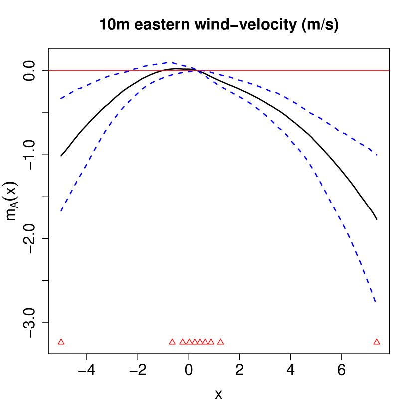
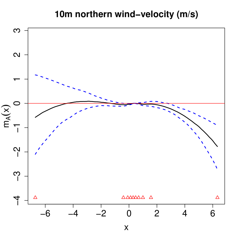
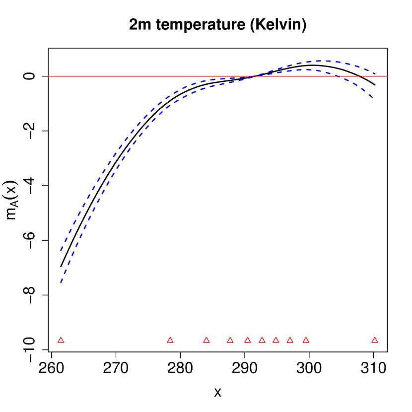
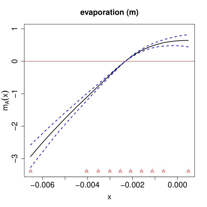
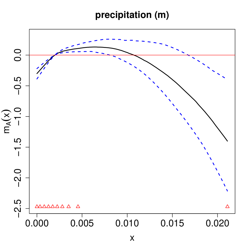
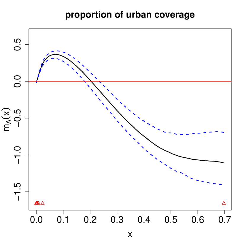
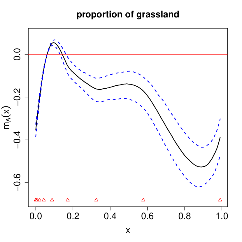
Figure 2: Estimated additive functions for $p_{0}(s,t)$. Blue dashed-lines give the $95\%$ confidence envelopes and the black solid line gives the median estimate over all bootstrap samples. Red triangles denote location of knots and the red lines intersect $m_{\mathcal{A}}(x)=0$.

Models for $p_{0}(s,t)$ are fitted by specifying $h_{i}$ in (3) as the logistic link function. Figure 2 gives the decomposition of the estimated additive function $m_{\mathcal{A}}$ for $p_{0}(s,t)$; each panel gives the individual contribution of one predictor to $m_{\mathcal{A}}$ and the $y$-axis scale indicates the contribution to the log-odds of monthly wildfire occurrence. Broadly speaking, we find that the first four interpreted predictors, e.g., both wind-velocity components, 2m temperature and evaporation, have the biggest impact on the occurrence probability of wildfires, which can be determined by the magnitude of the vertical scale on the figure panels. We determine if the effect of a predictor on $p_{0}(s,t)$ is significant by observing whether the confidence envelopes in Figure 2 include zero. The estimates suggest that the magnitude of wind-velocity is negatively associated with the log-odds of $p_{0}(s,t)$, with a stronger signal observed in the easterly component, and so we may expect windier months to experience less wildfires on average; however, this relationship only holds for strong easterly, westerly or northerly winds, as the effect of strong southerly winds seems to be insignificant. The observed effect of wind-speed is unusual; although it is well-known that high winds lead to increase wildfire spread (Abatzoglou et al., 2018), the effect on ignition is less well-studied. High winds can lead to power-line failure, which can cause wildfire ignition (Mitchell, 2013), as well as creating an abundance of oxygen; however, the temporal resolution of our data may be too coarse to observe these effects. Instead, we may be observing confounding between high wind-speeds and scarcity of fuel; for our data we observe that the largest wind-speeds typically occur along the south and south-west coastlines, as well as particularly mountainous regions, where fuel may not be as readily available. Both temperature and evaporation have a strong positive association with the log-odds of $p_{0}(s,t)$; months with higher temperature and a lower magnitude of evaporation are more likely to observe wildfires.

The remaining relationships are more difficult to infer; for precipitation, we observe that both large and small amounts of rainfall lead to decreases in $p_{0}(s,t)$. Wetter fuel is more difficult to ignite, which may explain the observed effects for very high rainfall, but the effect observed for the lower-tail is more difficult to explain. The relationship between wildfire occurrence and precipitation is complex; we associate low precipitation with wildfire occurrences as lightning-induced fires are more likely to occur with low-to-zero precipitation (Hall, 2007), but this relationship may be confounded by high temperatures, which facilitate convective precipitation (Kendon et al., 2014) and hence lead to higher monthly rainfall. Figure 2 suggests that temperature is a significant driver of wildfire occurrence, but we observe a slight decrease in the effect for very high temperatures; this may be an edge effect or it may be as a result of the higher precipitation rates that occur in hotter months. For the interpreted land coverage proportions, the effects of both urban and grassland on $p_{0}(s,t)$ is highly non-linear; for the former, we observe that highly built-up areas are much less likely to experience wildfires, which may be due to a scarcity of ignitable fuel. For intermediate values of urban coverage we observe a significant increase in the log-odds of $p_{0}(s,t)$ with an increase in the predictor, suggesting that wildfires are more likely to occur with a human presence; this is unsurprising, as it is well-known that human influence is one of the main causes of wildfires, see e.g., Vilar del Hoyo et al. (2011); Rodrigues and de la Riva (2014). For grassland proportion, we observe that low values give lower $p_{0}(s,t)$, suggesting that grassland may provide good fuel for wildfires. However, as the proportion increases above approximately $10\%$ the value of the log-odds of $p_{0}(s,t)$ begins to decrease; this may be due to a decrease in the abundance of fuels that burn more efficiently than grassland. Identifying such fuels using the current model specification is infeasible; to do so would require changing the predictors that compose $\mathbf{x}^{(i)}_{\mathcal{A}}(s,t)$, which could be done in a further study.

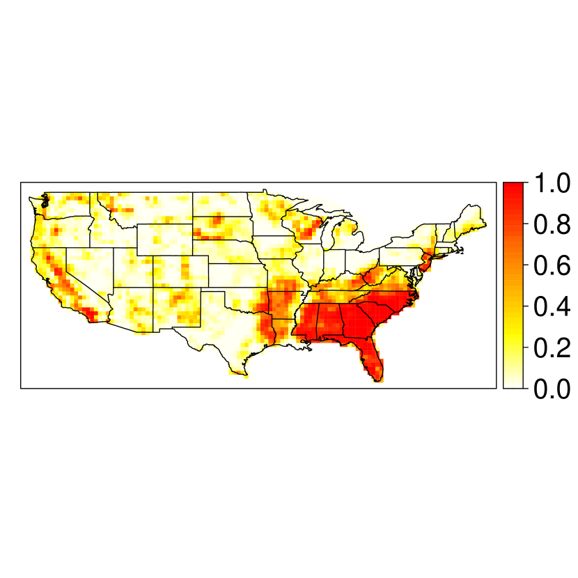
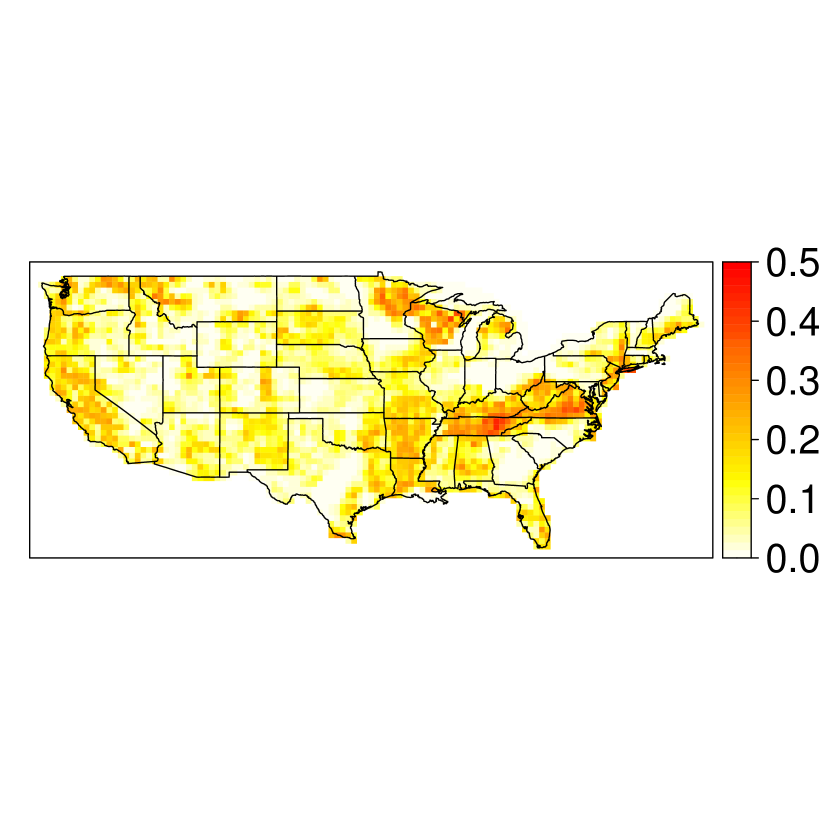
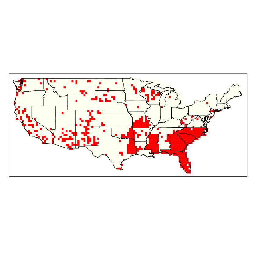
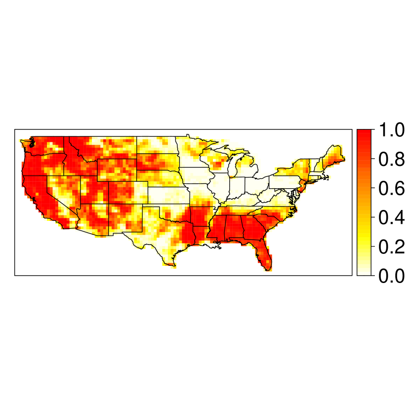
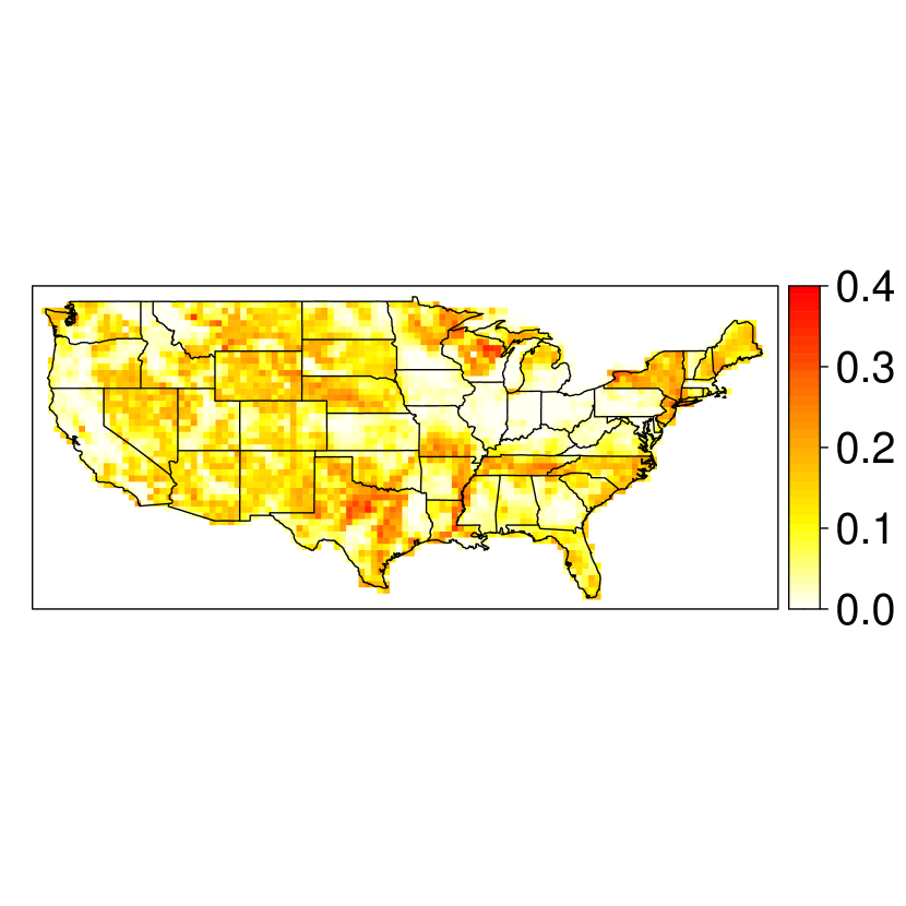
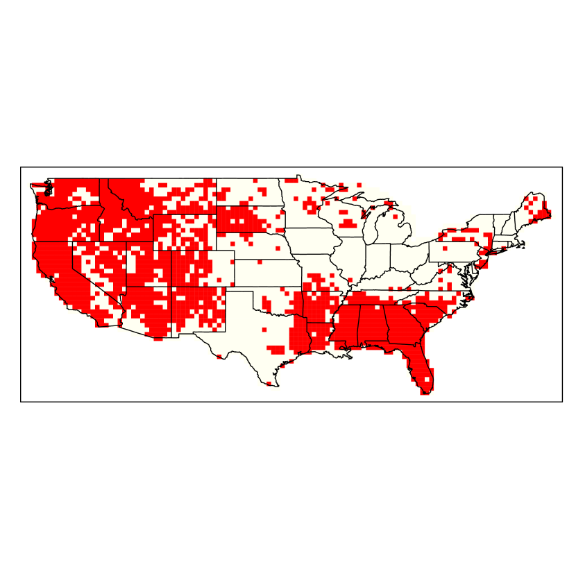
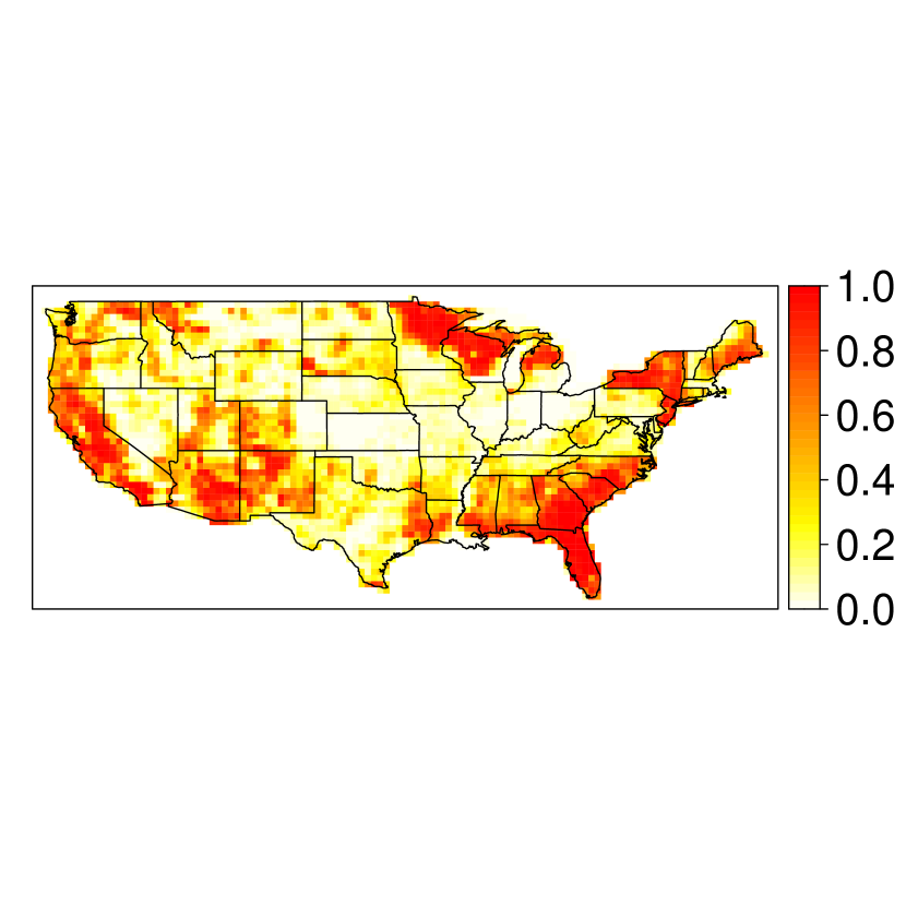
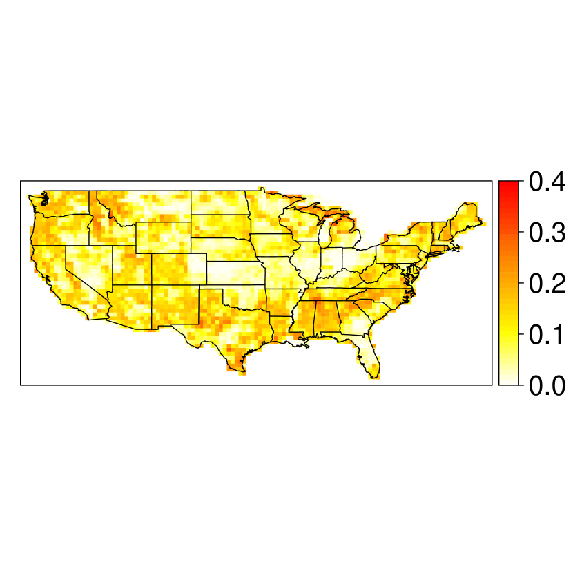
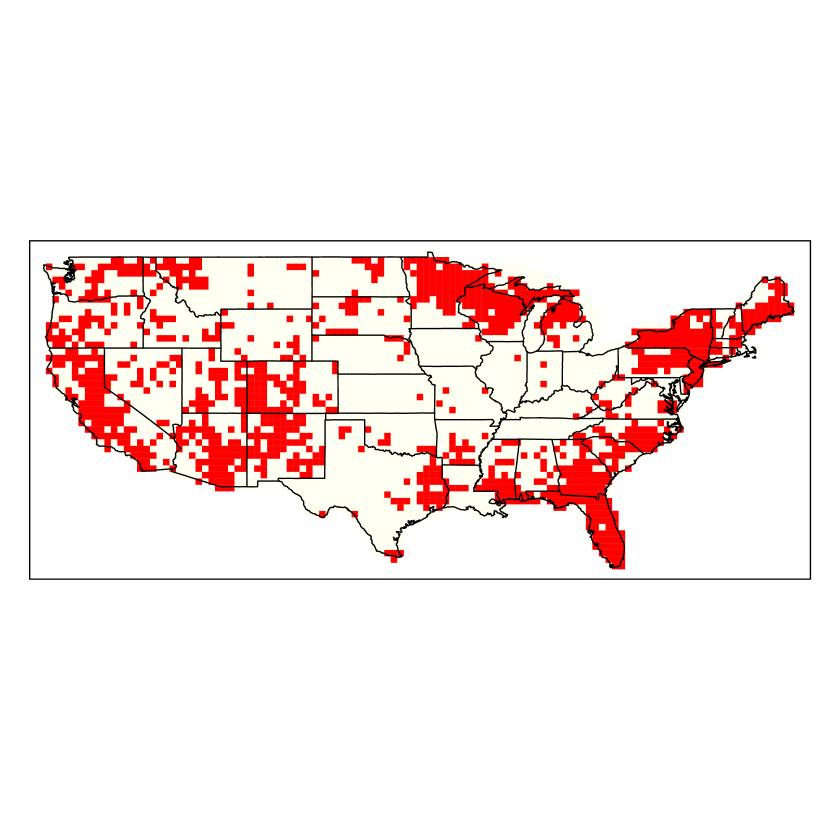
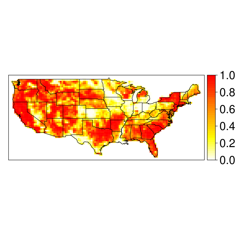
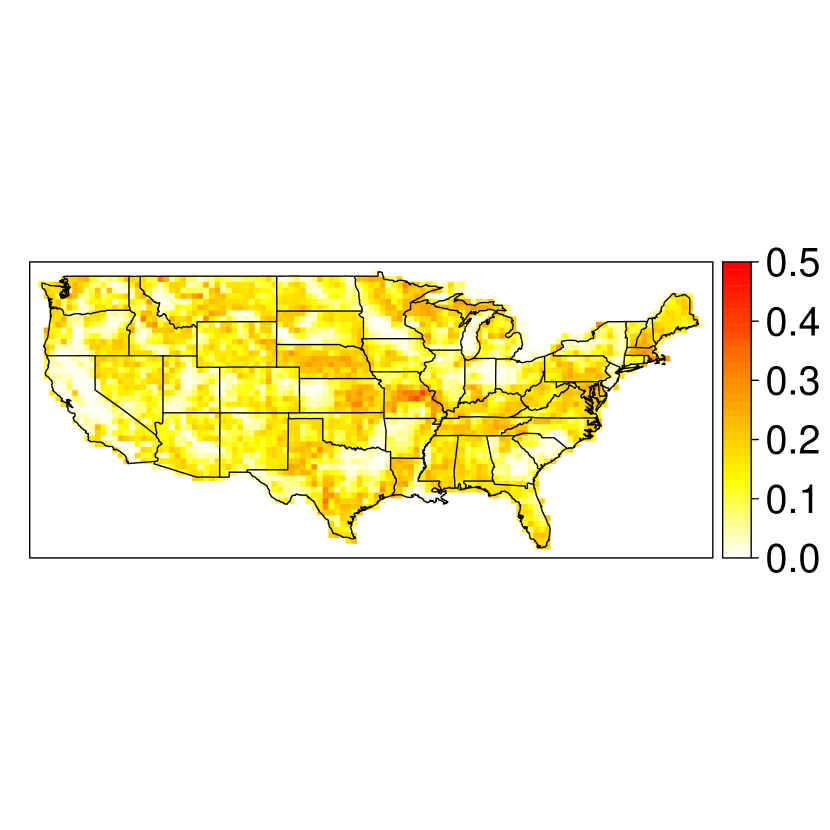
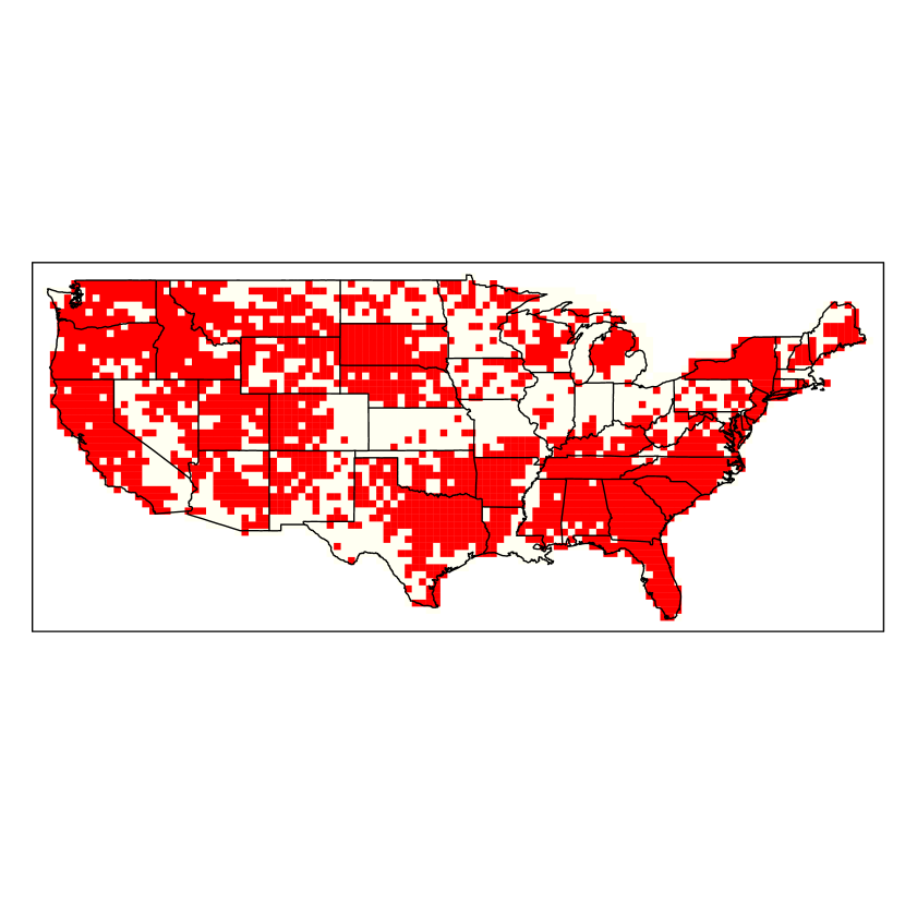
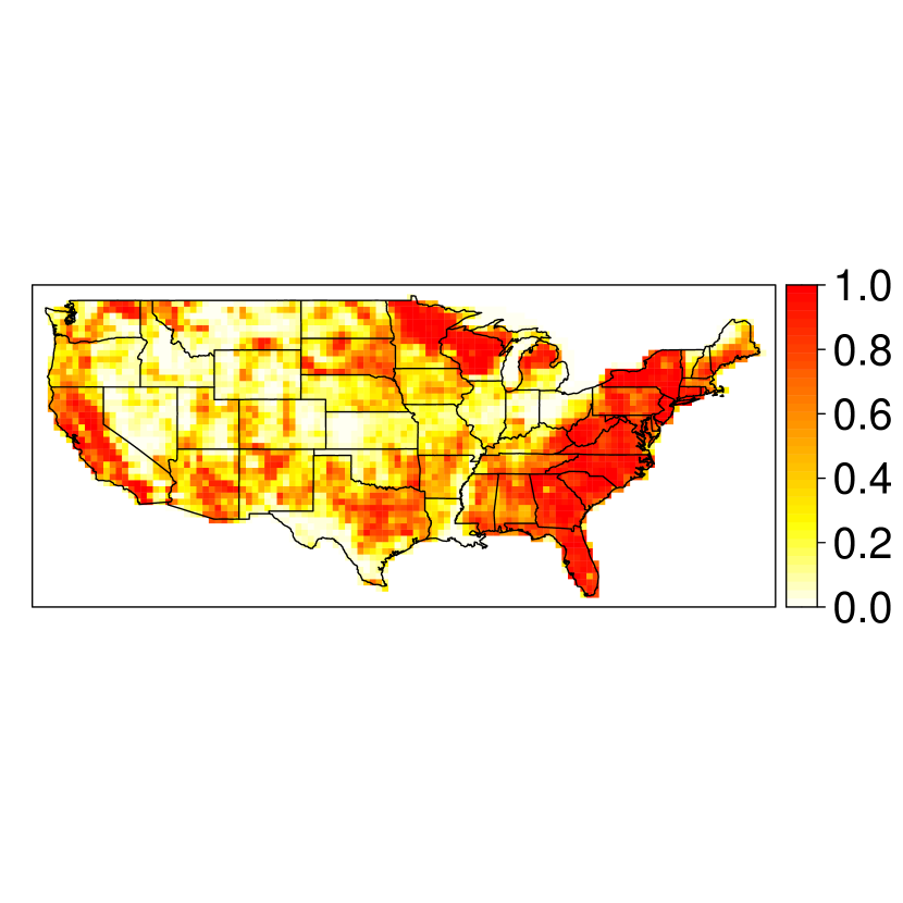
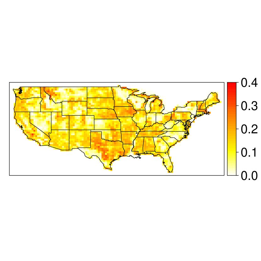
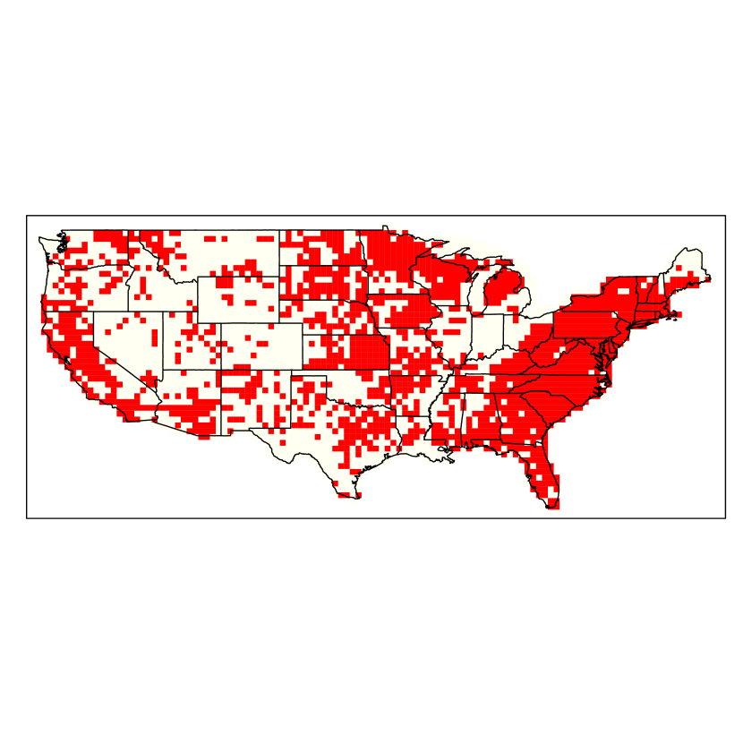
Figure S1: Maps of ${\rm Pr}\{Y(s,t)>0\mid\mathbf{X}(s,t)\}$ for different times $t$ (by row). Left and middle columns: estimated median and inter-quartile range, respectively, across all bootstrap samples. Right-column: observed wildfires (red). Times, top to bottom row: March 1993, August 2000, May 2003, July 2012, April 2015.

Figure 3 provides a map of the median estimated $p_{0}(s,t)$ for a fixed time $t$; for brevity, we consider here only the month July of 2007, as this month was the most devastating in terms of burnt area across the entire U.S., but maps for other selected months are provided in Figure S1. The maps of predicted probabilities match well with the observed wildfires, suggesting that the model fits well to the data. We observe large values of $p_{0}(s,t)$ across the entirety of the spatial domain, but particularly in the north-east, south-east, and western regions. Figure 3 further presents maps of uncertainty for estimates of wildfire occurrence probabilities, which we quantify using the inter-quartile range of $p_{0}(s,t)$ across bootstrap samples. As expected, we find that the grid-cells that produce the largest uncertainty are often those adjacent to regions that have experienced wildfires.

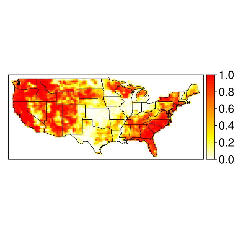
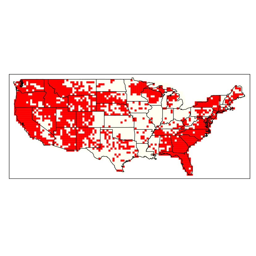
Figure 3: Maps of ${\rm Pr}\{Y(s,t)>0\mid\mathbf{X}(s,t)\}$ for July, 2007. Left and middle columns: estimated median and inter-quartile range, respectively, across all bootstrap samples. Right-column: observed wildfires (red).

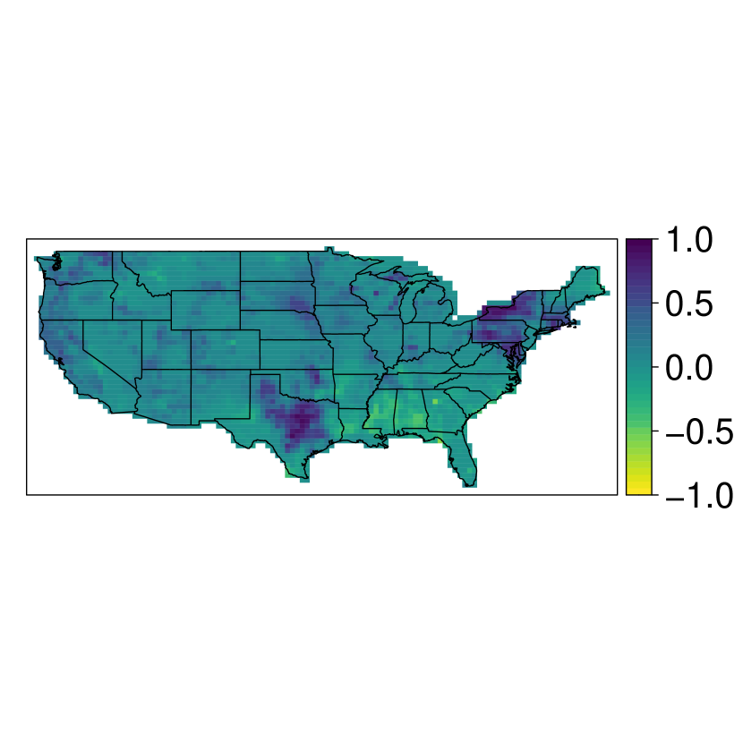
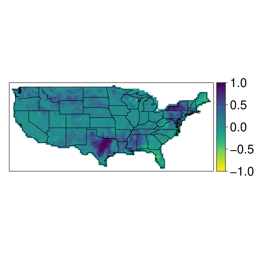
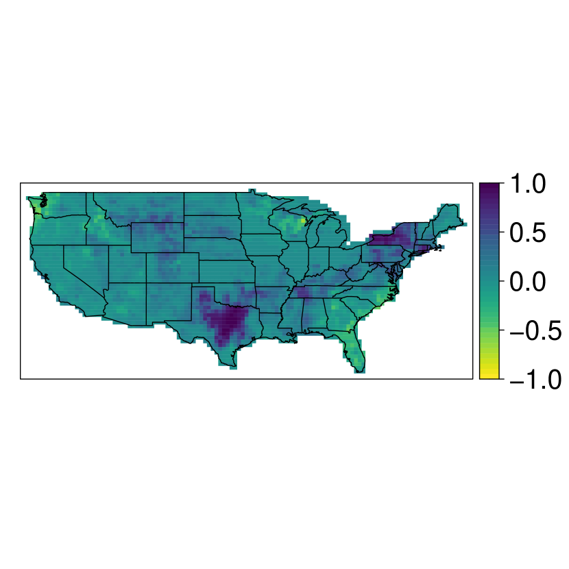
Figure S2: Maps of median site-wise differences in estimated $p_{0}(s,t)$ between the first and final years, stratified by month. From top-left to bottom-right, months are April-September.

To quantify temporal changes in $p_{0}(s,t)$, we present maps of the median site-wise differences in the estimates of $p_{0}(s,t)$ for the first and last years, stratified by month; three months are presented in Figure 4 with others in Figure S2. We generally observe that $p_{0}(s,t)$ increases during 1993–2015 for all months and for the vast majority of locations, suggesting that climate change may be exasperating the frequency of wildfires. Areas of particular concern include the north-western regions of the U.S. and Texas, which show large increases in $p_{0}(s,t)$ in the summer months (June-August) and the north-east, which shows increases in $p_{0}(s,t)$ in the colder months (March-May). Interestingly, parts of the eastern U.S. show a decrease $p_{0}(s,t)$ in some months, most obviously July, and the high-risk state of California does not show the significant increases observed elsewhere.

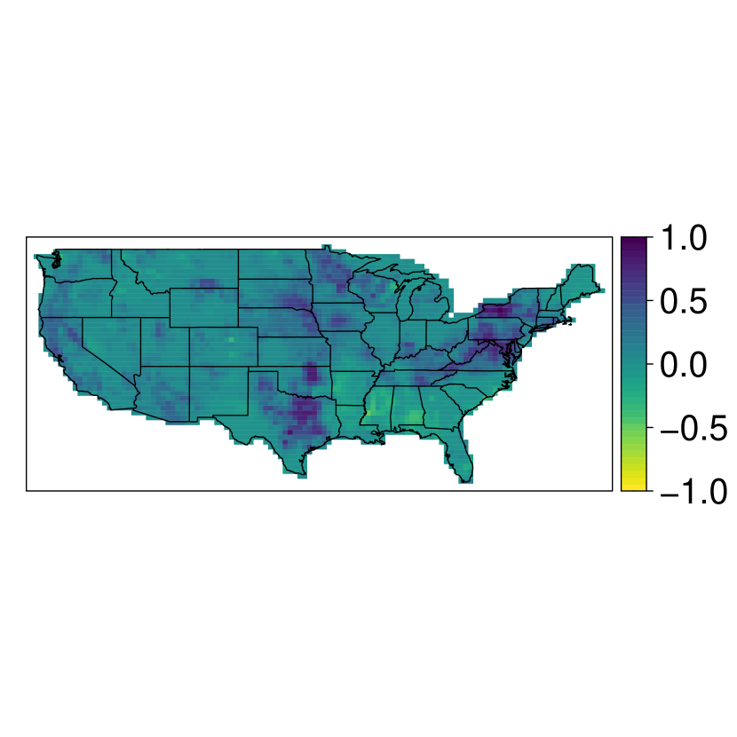
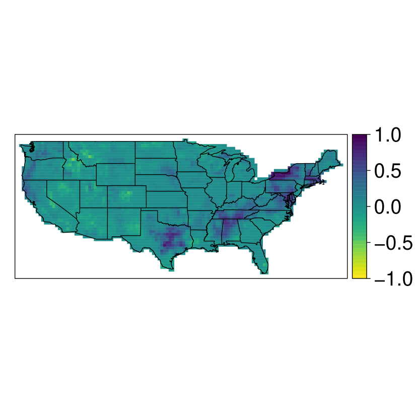
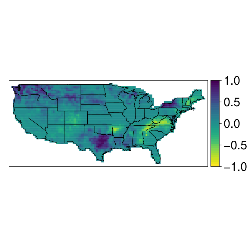
Figure 4: Maps of median site-wise differences in estimated $p_{0}(s,t)$ between the first and final years, stratified by month. Left-to-right: March, May, July.

4.3.3 Wildfire spread

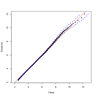
Figure S3: Q-Q plot for pooled bGEV-PP fit on standard Exponential margins, averaged across all bootstrap samples. $95\%$ tolerance bounds are given by the dashed lines. Black points give the median quantiles across all samples, with the quantile levels ranging from $0.9$ to a value corresponding to the maximum observed value.

To assess the fit and suitability of the bGEV-PP model to $\sqrt{Y}(s,t)\mid\{Y(s,t)>0,\mathbf{X}(s,t)\}$, we illustrate a pooled Q-Q plot in Figure S3 in Appendix E, transforming all data onto standard Exponential margins using the bGEV-PP fits; this procedure is repeated for each bootstrap sample and we observe good fits in the upper-tails as the estimated tolerance bands include the diagonal. The median of the shape parameter estimates (and $95\%$ confidence interval) is ${\widehat{\xi}}=0.359\;(0.342,0.372)$, suggesting that positive wildfire spread is particularly heavy-tailed; an observation also made by D’Arcy et al. (2021) and Koh (2021) for these data. Moreover the small confidence interval suggests that our assumption that $\xi$ is constant over space and time is well-founded. Note that this is an estimate of the the tail index for the square-root of the response, i.e., the burnt area “diameter", and so the area itself, $Y(s,t)$, will have even heavier tails and non-finite second-order moments.

We present median values of the estimated linear coefficients, i.e., $\boldsymbol{\eta}$ in (3) (and $95\%$ confidence intervals) for $q_{\alpha}$ and $s_{\beta}$. Note that the coefficients can be interpreted as the change to $q_{\alpha}(s,t)$ and $\log\{s_{\beta}(s,t)\}$, respectively, given an increase in the predictor value by one standard deviation and recall that $q_{\alpha}$ and $s_{\beta}$ correspond to the median and inter-quartile range of the annual maxima distribution associated with $\sqrt{Y}(s,t)\mid\{Y(s,t)>0,\mathbf{X}(s,t)\}$; thus, they can be interpreted as measures of the magnitude and variability of extreme wildfire spread, with both of their units being $\sqrt{\mbox{acres}}$. For $q_{\alpha}$, the estimated linear coefficients are $0.97\;(0.93,1.37)$, $0.93\;(0.91,1.06)$, $-0.01\;(-0.03,0.08)$ and $-0.01\;(-0.05,0.05)$ for 2m temperature, evaporation, precipitation and proportion of urban coverage, respectively, and similarly for $s_{\beta}$ we have $0.08\;(0.05,0.11)$ and $0.06\;(0.04,0.07)$ for 2m temperature and evaporation, respectively. We find a strong positive association of wildfire burnt area with temperature and evaporation for both $q_{\alpha}$ and $s_{\beta}$, suggesting that higher temperatures and lower evaporation magnitude lead to higher intensity and variability of extreme wildfires. We find no significant effect for precipitation and urban coverage on $q_{\alpha}$, as zero falls within the estimated $95\%$ confidence interval for both coefficients.

Figure 5 gives the decomposition of the estimated additive functions $m_{\mathcal{A}}$ for the two bGEV-PP model parameters. We begin by noting that all estimated functions appear non-linear, suggesting that linear models would be insufficient here; hence the necessity for the inclusion of the additive component in (3). The scales on the axes for $q_{\alpha}$ and $s_{\beta}$ correspond to a change in the value of $q_{\alpha}$ and $\log s_{\beta}$, respectively. We determine if the effect of a predictor on $q_{\alpha}$ or $s_{\beta}$ is significant by observing whether the confidence envelopes in Figure 5 include zero. We observe that, for both $q_{\alpha}$ and $s_{\beta}$, the effect of eastern wind-velocity appears to be insignificant; in the case of northern-wind velocity, we observe that high magnitude northern winds lead to a significant decrease in magnitude, but not variability, of extreme wildfires. The effect of grassland is highly non-linear; we observe that an increase in grassland proportion leads to a decrease in $s_{\beta}$, whereas the relationship between grassland and $q_{\alpha}$ is similar to that between grassland and $p_{0}(s,t)$ (see Figure 2). We observe that precipitation has the opposite effect on $s_{\beta}$ as it does for $p_{0}(s,t)$; small and large values of precipitation lead to a significant increase in wildfire variability. For proportion of urban coverage, there appears to be a significant increase in $s_{\beta}$ in highly built-up areas.

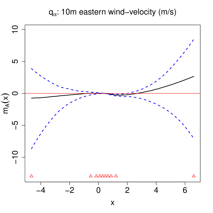
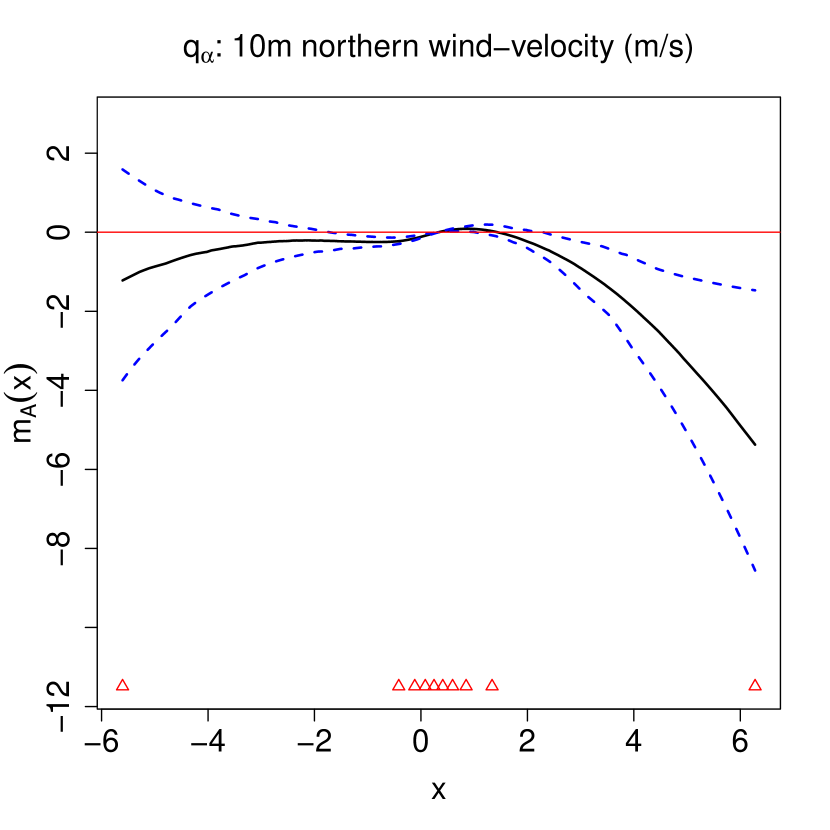
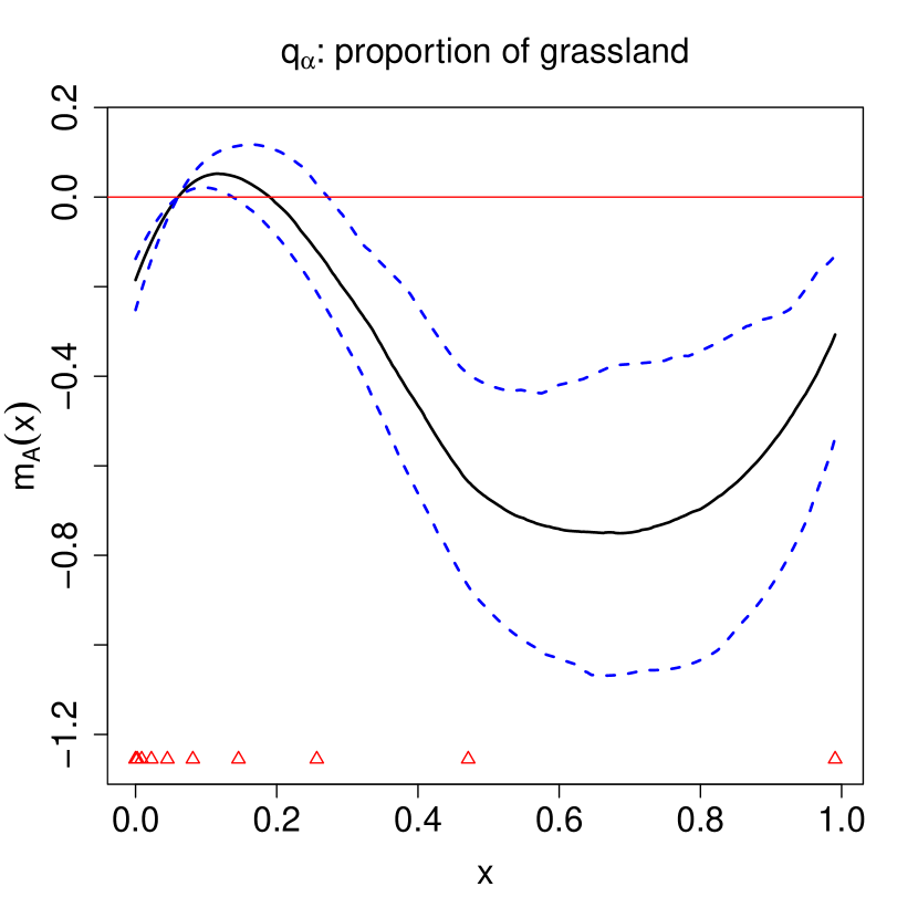
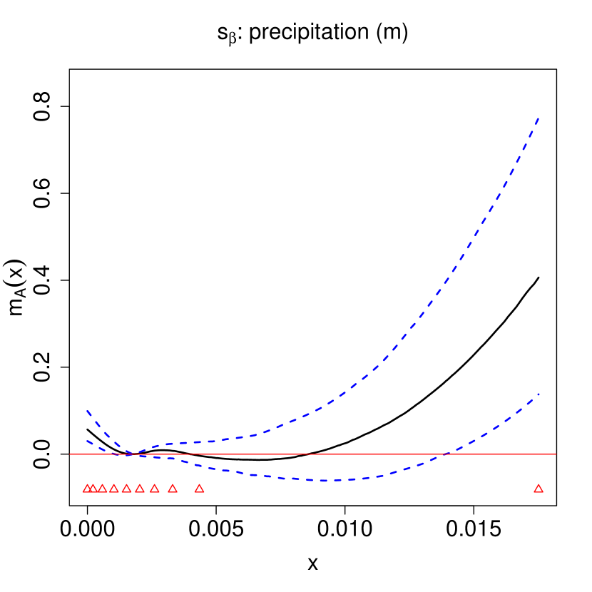
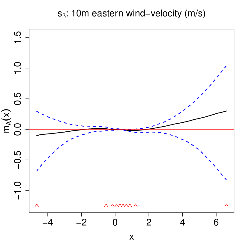
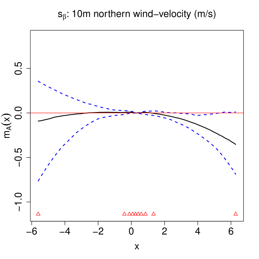
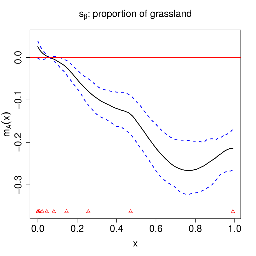
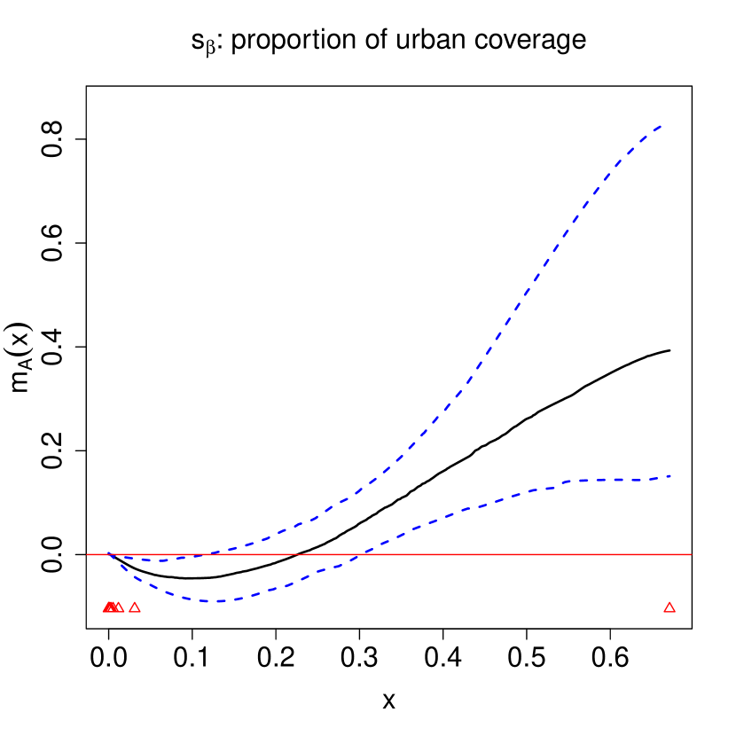
Figure 5: Decomposition of additive functions for $q_{\alpha}$ (top row, columns 1-3) and $s_{\beta}$. Blue dashed-lines give $95\%$ confidence envelopes and the black solid line gives the median estimate over all bootstrap samples. Red triangles denote location of knots and the red lines intersect $m_{\mathcal{A}}(x)=0$.

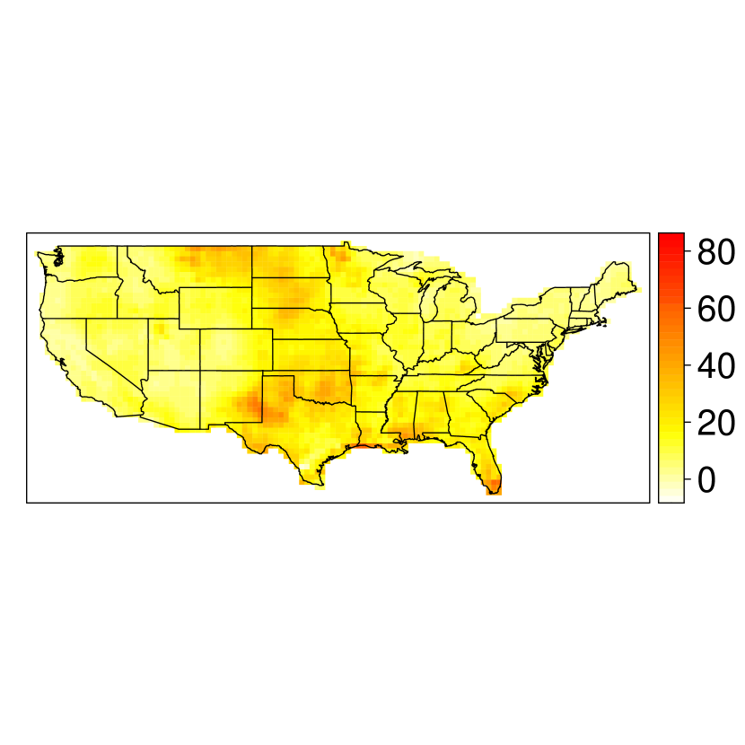
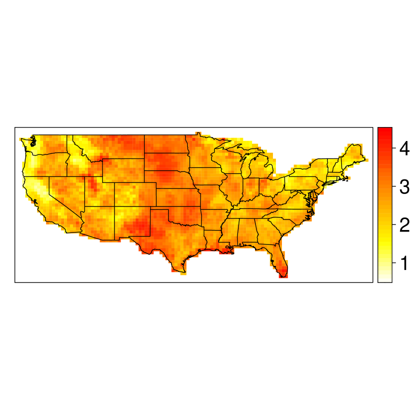
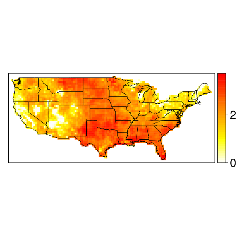
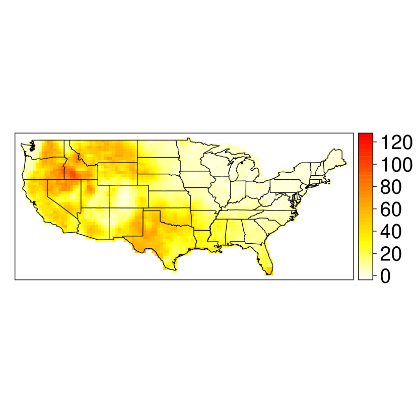
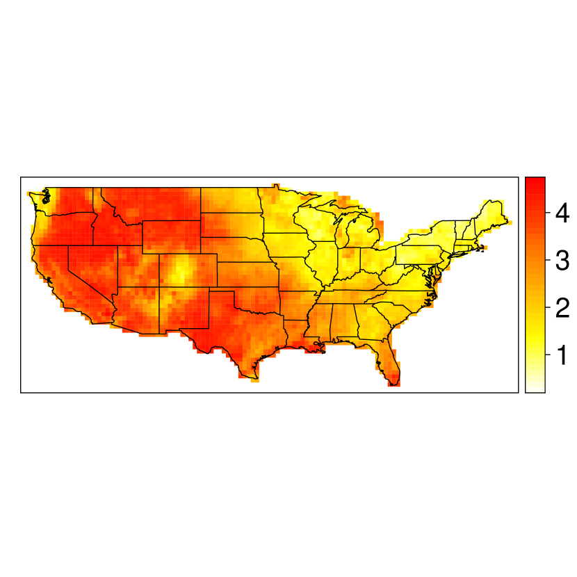
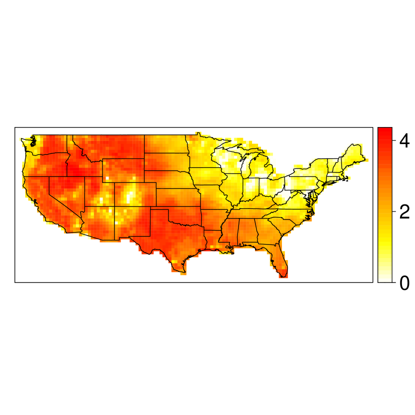
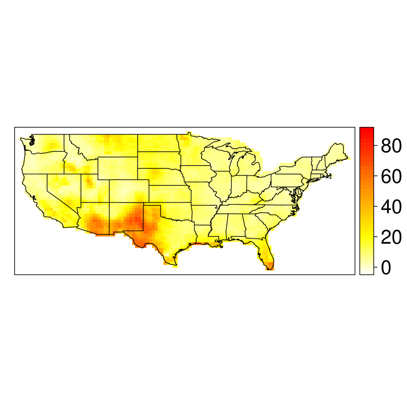
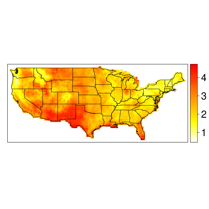
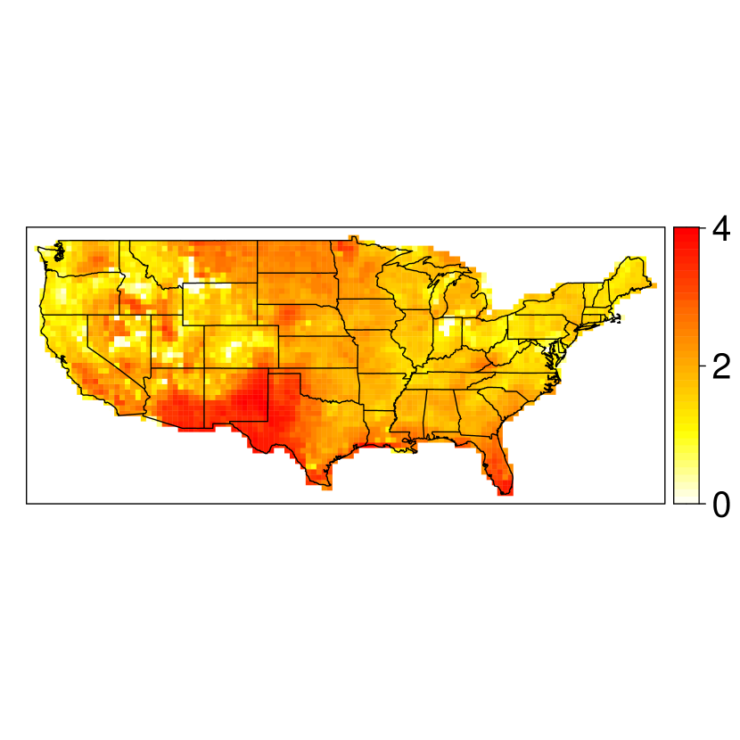
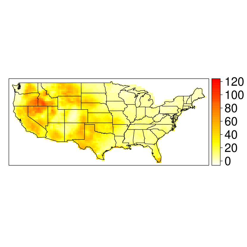
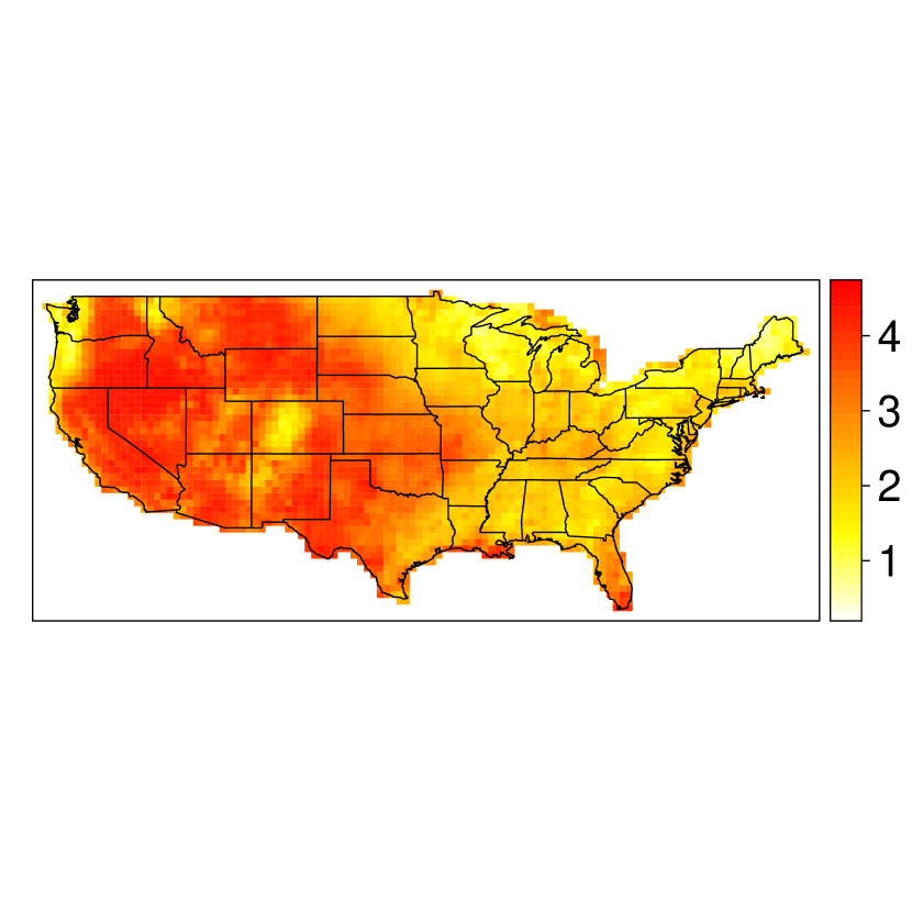
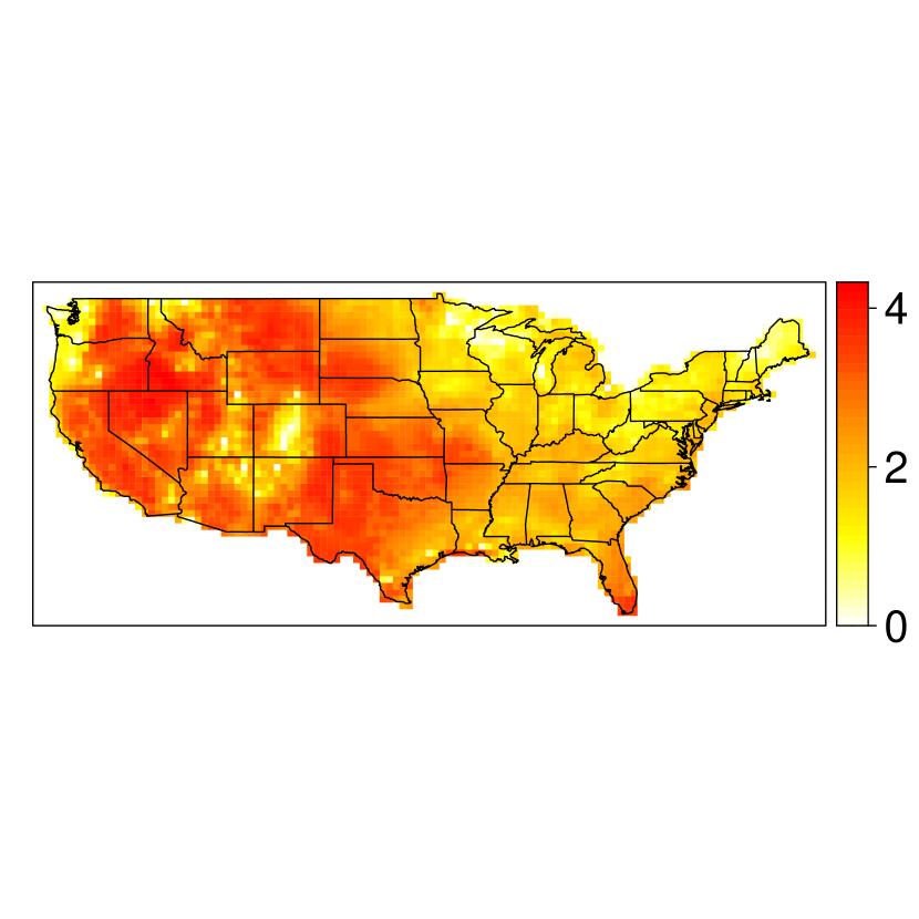
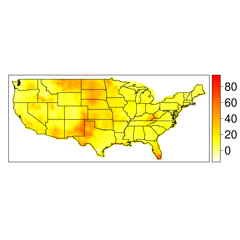
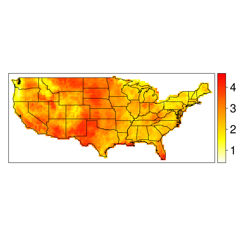
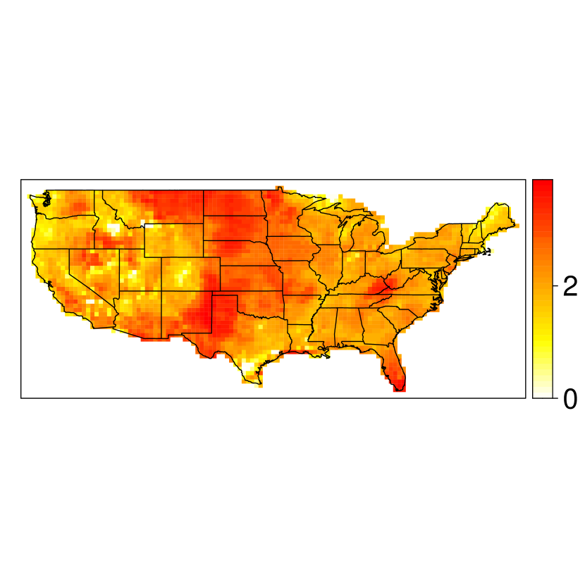
Figure S4: Maps of median estimated $q_{\alpha}(s,t)$ (left), $\log(1+s_{\beta}(s,t))$ (middle) and $90\%$ quantile of $\log(1+Y(s,t))\mid(Y(s,t)>0,\mathbf{X}(s,t))$ (right) for different times $t$ (by row). Times, top to bottom row: March 1993, August 2000, May 2003, July 2012, April 2015.

Figure 6 provides maps of the estimated bGEV-PP location and spread parameters, as well as the $90\%$ quantile of $\sqrt{Y}(s,t)\mid\{Y(s,t)>0,\mathbf{X}(s,t)\}$, for July 2007; similar maps for other months are provided in Figure S4. We generally observe that the magnitude and variability of wildfire spread are intrinsically linked; areas of large $q_{\alpha}$ typically occur with large $s_{\beta}$. For July 2007, large values of $q_{\alpha}$ tend to occur in the western areas of the U.S., including California, whilst large values of $s_{\beta}$ occur over a larger region that stretches into the centre of the domain. Although we do not observe large values of $q_{\alpha}$ in the east, we still observe high estimates of the $90\%$ quantile there, due to the effect of $s_{\beta}$. Note that the presented quantiles are for strictly positive spread only, and so do not necessarily characterise the overall, or compound, risk of wildfire burnt area. Instead these maps can be used to identify areas where it is most pertinent to prevent wildfires. For example, there are regions for which Figure 3 suggests that there is a low probability of wildfire occurrence, whilst Figure 6 illustrates that the spread distribution there is particularly extreme, e.g., parts of California, Nevada, northern Texas; hence it is important to prevent wildfires in those regions as, if they were to occur, they would be particularly devastating.

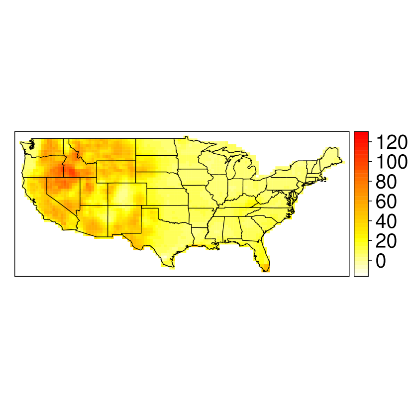
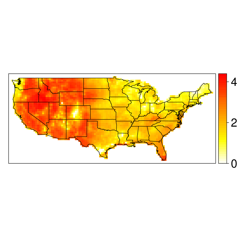
Figure 6: Maps of median estimated $q_{\alpha}(s,t)$ (left), $\log(1+s_{\beta}(s,t))$ (middle) and $90\%$ quantile of $\log(1+\sqrt{Y}(s,t))\mid\{Y(s,t)>0,\mathbf{X}(s,t)\}$ (right) for July, 2007.

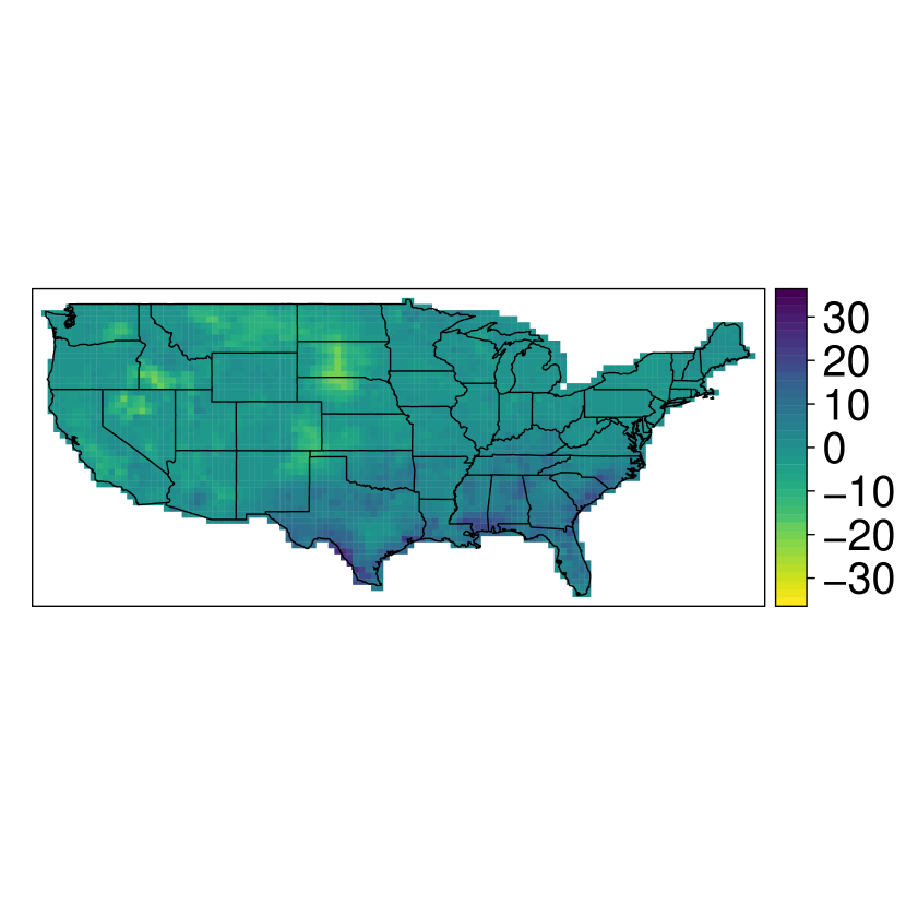
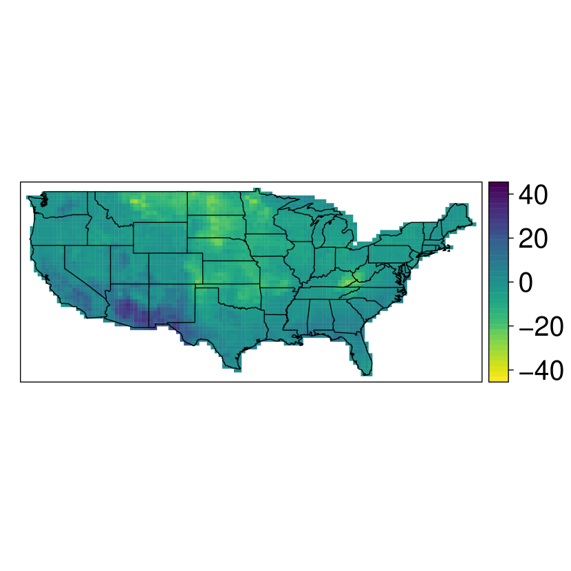
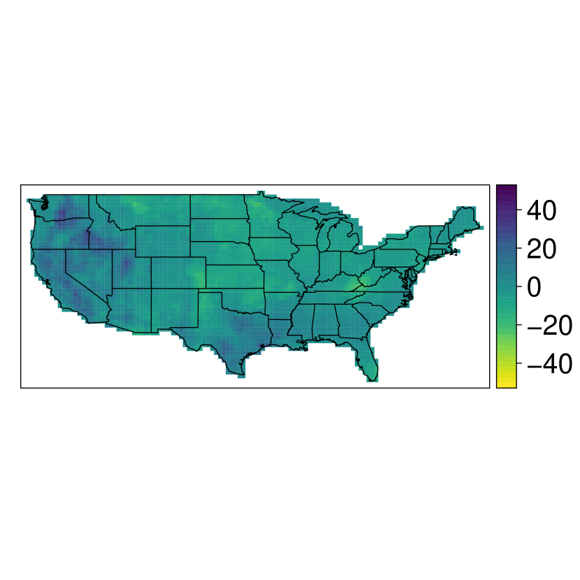
Figure S5: Maps of median site-wise differences in estimated $90\%$ quantile of $\log(1+\sqrt{Y}(s,t))\mid\{Y(s,t)>0,\mathbf{X}(s,t)\}$, stratified by month. From top-left to bottom-right, April to September.

Figure 7 present maps of median site-wise differences in the estimates of the $90\%$ quantile of $\sqrt{Y}(s,t)\mid\{Y(s,t)>0,\mathbf{X}(s,t)\}$ for the first and last years, stratified by months; three months are presented in Figure 7 with other presented in Figure S5. We observe decreases in quantile for the spread distribution across large parts of the U.S, suggesting reductions in the severity of wildfires in these areas. However, we do observe large increases in the quantiles for the south-east during March, as well as in the western U.S. and Texas for the warmer months (June-September).

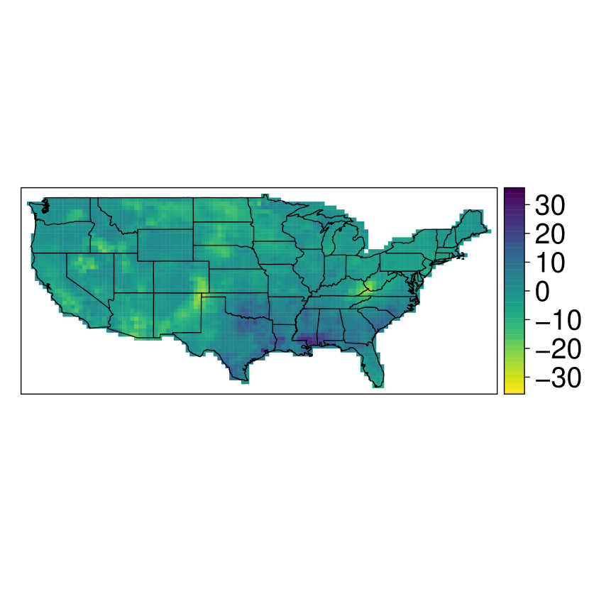
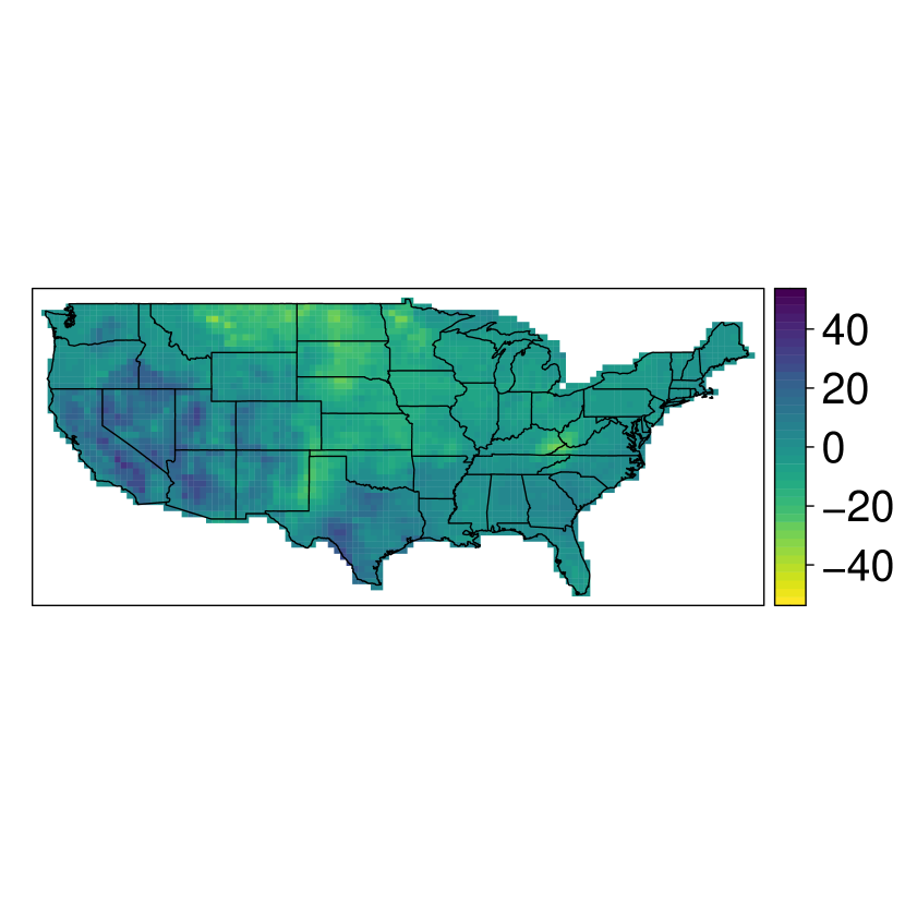
Figure 7: Maps of median site-wise differences in estimated $90\%$ quantile of $\log(1+\sqrt{Y}(s,t))\mid\{Y(s,t)>0,\mathbf{X}(s,t)\}$, stratified by month: March (left), May (centre), July (right).

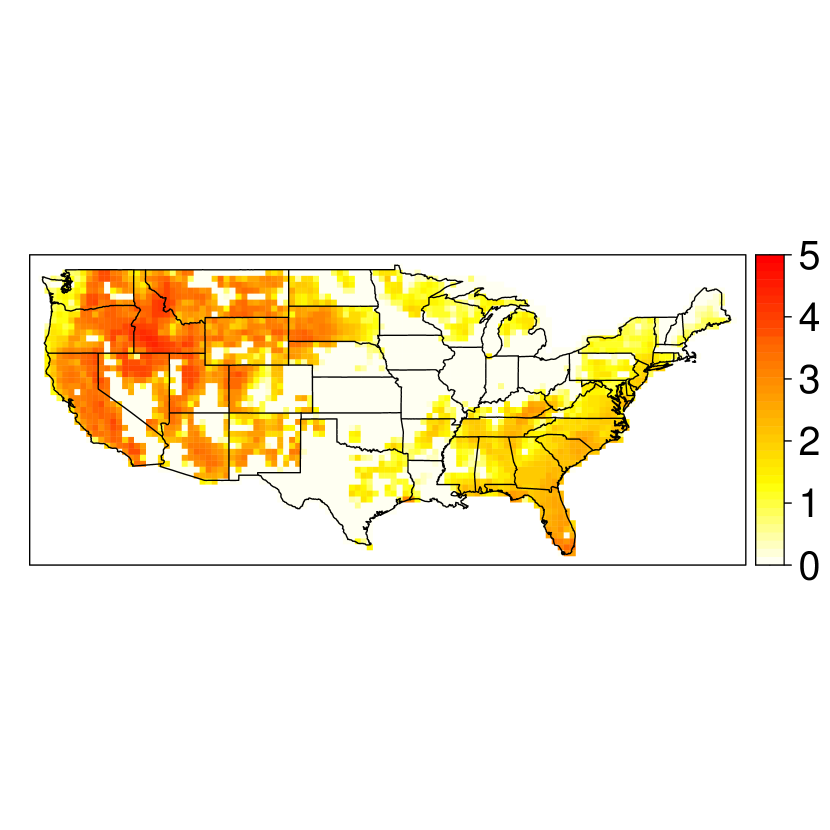
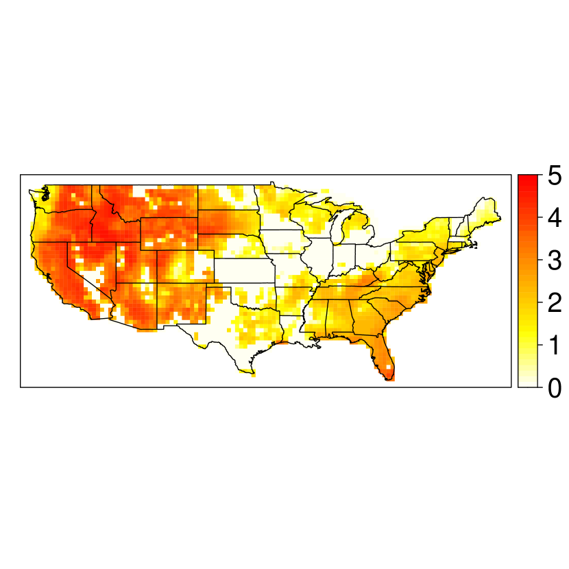
Figure 8: Maps of median estimated quantiles for $\log(1+\sqrt{Y}(s,t))\mid\mathbf{X}(s,t)$ for July 2007. Quantiles, left to right: $90\%$, $95\%$ and $99\%$.

Figure 8 provides maps of estimated extreme quantiles for $\log(1+\sqrt{Y}(s,t))\mid\mathbf{X}(s,t)$, i.e., the unconditional response, in July 2007, which characterises compound risk for this month, i.e., the overall risk of burnt area. We note that areas of large values in Figure 8 do not necessarily correspond to areas of large values in Figure 3 or Figure 6 and so we conclude that the spread and occurrence of wildfires are not intrinsically linked; different factors lead to wildfire ignition as well as spread, and so our decision to model both processes separately is well-founded. We observe high values of the quantiles across large areas of the U.S., typically in the west of the U.S., including California, and the south-east, including Florida, with states in the north-east, and Texas, having relatively low compound risk.

5 Discussion

We have proposed a framework for performing semi-parametric extreme quantile regression using partially-interpretable neural networks. The methodology unifies the tail robustness and theoretical strength of parametric EV models, the high predictive accuracy and computational efficiency of neural networks, and the interpretability of linear and spline-based regression models, allowing us to accurately estimate extreme quantiles whilst simultaneously performing statistical inference. To complement this flexible methodological framework, we propose a new point process model for extreme values that circumvents issues concerning finite lower-bounds on the process intensity function, which is a key issue when training neural networks. We use a large ensemble of neural networks to model the compound risk of extreme wildfires in the contiguous U.S., with separate models proposed for the occurrence and spread of extreme wildfires. Our approach allows for the identification of high-risk areas of the U.S., as well as facilitating inference that reveals interesting insight into the driving behaviour of wildfires, which is important for risk assessment and mitigation.

Sections 4.3 and Appendix C.2 highlight the predictive power of convolutional networks, which are capable of capturing spatial patterns in predictors, when they are applied to our data; we capitalise on their performance in our analyses in Section 4.3. A drawback of CNNs (and the recurrent neural networks we tried) is that they are only applicable to gridded data, which has been constructed as a sequence of images. Moreover, they can suffer from edge effects if the convolutional filters must pass outside of the spatial domain $\mathcal{S}$; recall that predictor values for locations that lie outside of $\mathcal{S}$ are set to zero, i.e., the mean of the predictor across all space-time locations. Hence, future studies may benefit from using alternatives to the CNN. For example, Scarselli et al. (2008) propose graphical neural networks (GNNs), which are applicable to data with a graphical structure. Recent developments (see review by Zhou et al. (2020)) of GNNs have seen the proposal of convolutional (Kipf and Welling, 2016) and recurrent (e.g., Li et al. (2015)) extensions that can handle data which are irregularly-spaced throughout $\mathcal{S}$ and $\mathcal{T}$, respectively; hence they could be used in our framework to model the extremes of processes observed at point locations or on irregularly-spaced grids.

We consider one type of extreme response distribution EV for modelling, namely the newly proposed bGEV-PP model. However, our framework extends far beyond the use of this specific model; EV can be replaced by any parametric model. For example, it is trivial to see how EV could be the bGEV distribution; we would model block-maxima of the response and appropriately aggregate the predictors. As is common with many extreme value approaches, fitting of the bGEV-PP and GPD models requires a prerequisite step whereby a sufficiently high threshold $u(s,t)$ is estimated; $u(s,t)$ is typically estimated to ensure a constant exceedance probability ${\rm Pr}\{Y(s,t)>u(s,t)\}$ across all $(s,t)\in\mathcal{S}\times\mathcal{T}$. When modelling the response below $u(s,t)$, the bGEV-PP model performs poorly and the GPD fails altogether; alternatives that can be used to model both the upper-tails of the response, as well as the bulk, are mixture models with GPD tails, see, e.g., Carreau and Bengio (2007) and Carreau and Vrac (2011), but these still require specification of $u(s,t)$. Estimating $u(s,t)$ requires additional modelling choices and can contribute to the model uncertainty for EV; Papastathopoulos and Tawn (2013); Naveau et al. (2016) and Yadav et al. (2021) propose extensions of the GPD which model the whole distribution and removes this requirement, and so may provide better candidates for EV than both the GPD and bGEV-PP.

Finally, to make our unifying partially-interpretable neural network (PINN)-based framework for extreme quantile regression available to the whole statistical community at large, and for reproducibility, we have created the R package pinnEV (Richards, 2022).

Appendices

Appendix A Modelling covariate-dependent parameters

A.1 Connection to main text

This appendix supports the material in Section 1.5 of the main paper. Appendix A.2 and Appendix A.3 detail the generalised additive framework and neural networks used in model (3) of the main text.

A.2 Generalised additive models

Following Wood (2006), a generalised additive model (GAM) allows parameters to be represented through a basis of splines, creating a smooth function of predictors; we apply this approach to model the function $m_{\mathcal{A}}$ in (3). Given a set of $a$ predictors $x_{1}(s,t),\dots,x_{a}(s,t)$, we can define $k_{i}\in\mathbb{N}$ knots for each predictor by $\{x^{*i}_{1},\dots,x^{*i}_{k_{i}}\}$ for $i=1,\dots,a$. We then let

$$m_{\mathcal{A}}(s,t)=\sum^{a}_{i=1}\sum^{k_{i}}_{j=1}w_{ij}\psi_{ij}(x_{i}(s,t),x_{j}^{*i}),$$ (S.1)

where $w_{ij}\in\mathbb{R}$ for all $i=1,\dots,a,j=1,\dots,k_{i}$ and where $\psi_{ij}$ are arbitrary smoothing basis functions. We constrain our focus to the simple case where $\psi_{ij}(x,y)=\psi(x,y)=\|x-y\|^{2}\log\|x-y\|$ for all $i,j$ and where $\|\cdot\|$ denotes the Euclidean norm, i.e., each $\psi$ is a radial basis function and $m_{\mathcal{A}}$ is a thin-plate spline (Wood, 2003), and fix $k_{i}=k$ for all $i=1,\dots,a$.

If required, a smoothing penalty can be accommodated into the loss, or negative log-likelihood, function to ensure that the splines are smooth enough (Silverman, 1985). For smoothness parameters $\boldsymbol{\lambda}=(\lambda_{1},\dots,\lambda_{a})>\mathbf{0}$ and with $\boldsymbol{\omega}=(\boldsymbol{\omega}^{T}_{1},\dots,\boldsymbol{\omega}_{a}^{T})^{T}$ where $\boldsymbol{\omega}_{i}=(\omega_{i1},\dots,\omega_{ik_{i}})^{T}$, we add $\boldsymbol{\omega}^{T}S_{\boldsymbol{\lambda}}\boldsymbol{\omega}/2$ to the loss, where $S_{\boldsymbol{\lambda}}=\sum^{a}_{i=1}\lambda_{i}S_{i}$ and $S_{i}$ is an $|\boldsymbol{\omega}|\times|\boldsymbol{\omega}|$ matrix with all zero entries except for a $k_{i}\times k_{i}$ block, denoted $S_{i}^{*}$, which begins at the $[\sum^{i-1}_{j=1}k_{i}+1,\sum^{i-1}_{j=1}k_{i}+1]$-th entry of $S_{i}$ if $i>1$ and the $[1,1]$-th entry, otherwise. The $[j,k]$-th entry of $S_{i}^{*}$ is given by $\psi(x_{j}^{*i},x_{k}^{*i})$.

A.3 Neural networks

A.3.1 Overview

We describe a neural network with $J$ hidden layers, each with $n_{j}$ neurons for $j=1,\dots,J$, and with a set of $d$ predictors $\mathbf{x}(s,t)=(x_{1}(s,t),\dots,x_{d}(s,t))$ for $(s,t)\in\mathcal{S}\times\mathcal{T}$. The output for layer $j$ and neuron $i$ is described by the function $m_{j,i}(s,t)$, which differs for the three considered layer types (MLP, CNN and LSTM). Defining the vector of outputs from layer $j$ by $\mathbf{m}_{j}(s,t)=(m_{j,1}(s,t),\dots,m_{j,n_{j}}(s,t))$, then the output layer, i.e., $m_{\mathcal{N}}$ in (3) of the main text, can always be described by

$$m_{\mathcal{N}}(\mathbf{x}(s,t))=(\mathbf{w}^{(J+1)})^{T}\mathbf{m}_{J}(s,t),$$

for weight vector $\mathbf{w}^{(J+1)}\in\mathbb{R}^{n_{J}}$. We now describe the possible choices for the output of the nodes in the $j$-th layer, which is determined by one of three classes; densely-connected, convolutional, or recurrent, layers.

A.3.2 Densely-connected layers

If the $j$-th layer is densely-connected, i.e., from an MLP, then the output is simply a weighted sum of the outputs from the previous layer; the output at each node $i=1,\dots,n_{j}$ is

$$m_{j,i}(s,t)=h_{j}\left\{b^{(j,i)}+(\mathbf{w}^{(j,i)})^{T}\mathbf{m}_{j-1}(s,t)\right\},$$ (S.2)

for bias $b^{(j,i)}\in\mathbb{R}$, weights $\mathbf{w}^{(j,i)}\in\mathbb{R}^{n_{j-1}}$ and fixed activation function $h_{j}$, with the convention that $m_{0,i}(s,t):=x_{i}(s,t)$ for $i=1,\dots,d$. The activation function is typically non-linear, and many choices can be considered (Ramachandran et al., 2017). Throughout we use only the rectified linear unit (ReLu) activation function, defined by $h_{j}(x)=\max\{0,x\}$, as Glorot et al. (2011) illustrates that they lead to better predictive performance than alternatives. Moreover, they can emulate the capabilities of biological neurons by “switching off" if the input value is too small, and they are computationally efficient.

A.3.3 Convolutional layers

We note that convolutional layers are only applicable if $\mathcal{S}$ can be represented as a $D_{1}\times D_{2}$ grid of locations. If this is the case, then a convolution filter is created, with pre-specified dimension $d_{1,j}\times d_{2,j}$ for $d_{1,j},d_{2,j}$ odd integers, $d_{1,j}\leq D_{1},d_{2,j}\leq D_{2}$; this filter is then applied over the input map. We define a neighbourhood $\mathcal{N}_{j}(s)$ as the locations $\{s\in\mathcal{S}\}$ such that they form a $d_{1,j}\times d_{2,j}$ grid with site $s$ at the centre and let $M^{(j-1,i)}(s,t)$ be a $d_{1,j}\times d_{2,j}$ matrix created by evaluating $m_{j-1,i}(s,t)$ on the grid $\mathcal{N}_{j}(s)$. For a $d_{1,j}\times d_{2,j}$ weight matrix $W^{(j,i)}$ with real entries, the $i$-th convolutional filter for layer $j$ is then of the form $\mathcal{C}_{j,i}(m_{j-1,i}(s,t))=\sum_{k=1}^{d_{1,j}}\sum_{l=1}^{d_{2,j}}W^{(j,i)}[k,l]M^{(j-1,i)}(s,t)[k,l]$ with operations taken entry-wise; here $A[k,l]$ denotes the $(k,l)$-th entry of matrix $A$. Then if layer $m_{j,i}(s,t)$ is convolutional, it takes the form

$$m_{j,i}(s,t)=h_{j}\left\{b^{(j,i)}+\sum^{n_{j-1}}_{k=1}\mathcal{C}_{j,k}(m_{j-1,k}(s,t))\right\},$$ (S.3)

for $i=1,\dots,d$; equivalence with the densely-connected layers is achieved by setting $d_{1,j}=d_{2,j}=1$.

To ensure that the convolutional filter can be applied at the boundaries of $\mathcal{S}$, we pad the predictor maps by mapping $\mathcal{S}$ to a new domain $\mathcal{S}^{*}$, a $(D_{1}+\max_{j=1,\dots,J}\{d_{1,j}\}-1)\times(D_{2}+\max_{j=1,\dots,J}\{d_{2,j}\}-1)$ grid with $\mathcal{S}$ at the centre. Then, for all $i=1,\dots,p$, we set $\mathbf{x}_{i}(s,t)=0$ for all $s$ within distance $(\max_{j=1,\dots,J}\{d_{1,j}\}-1)/2$ and $(\max_{j=1,\dots,J}\{d_{2,j}\}-1)/2$ of the first and second dimension, respectively, of the boundaries of $\mathcal{S}^{*}$.

A.3.4 Recurrent layers

The premise of a recurrent layer is that the $j$-th layer applied at time $t$ incorporates information from the $(j-1)$-th layer at time $t$ as well as information from the $j$-th layer at the $(t-1)$-th input. Networks using these layers can model $Y(s,t)$ given not only the predictor set $\mathbf{x}(s,t)$ at a single time $t$, but also given the rest of the time series information of the predictor, i.e., $\{\mathbf{x}(s,t):t\in\mathcal{T}\}$. We present here a simple recurrent layer for illustration purposes; in our application, we use LSTM layers which are more numerically stable, but for brevity we omit their details and direct the reader to Hochreiter and Schmidhuber (1997).

A recurrent layer involves the application of a densely-connected or CNN layer recurrently over a finite time period relative to the input time $t$; we denote this time period $[t-\tau_{1},t+\tau_{2}]$ for $\tau_{1},\tau_{2}>0$. Hence, recurrent layers cannot be used for estimation of parameters $\theta_{i}(s,t^{*})$ if $t^{*}-\tau_{1}\leq 0$ or $t^{*}+\tau_{2}>\max_{t\in\mathcal{T}}\{t\}$; in such cases, the response variables $\{Y(s,t^{*})\}$ must be removed from the analysis. The input and output of a recurrent layer is dependent on whether the preceding and subsequent layers, respectively, are also recurrent; for the output of the $j$-th recurrent layer and for node $i=1,\dots,n_{j}$, we let

$$m^{*}_{j,i}(s,t) =h_{j}\{b^{(j,i)}+f_{j,t}(\boldsymbol{m}^{+}_{j-1}(s,t))+f^{*}_{j,t-1}(\boldsymbol{m}^{*}_{j}(s,t-1))\},$$ (S.4)

for ${\boldsymbol{m}^{*}_{j}(s,t)=(m^{*}_{j,1}(s,t),\dots,m^{*}_{j,n_{j}}(s,t))}$ and bias term $b^{(j,i)}\in\mathbb{R}$ and where $m^{+}_{j-1,i}(s,t):=m^{*}_{j-1,i}(s,t)$ if the $(j-1)$-th layer is recurrent, and $m^{+}_{j-1,i}(s,t):=m_{j-1,i}(s,t)$, otherwise. The recursive relationship given in (S.4) can only be applied to a finite subset of $\mathcal{T}$ and in application it may be unreasonable to assume that the predictors at time $t^{*}$ affect the response at time $t$ if $|t-t^{*}|$ is large, so we set $f^{*}_{j,t^{*}}(\mathbf{m}^{*}_{j}(s,t))=0$ for all $s\in\mathcal{S}$ and $t^{*}\leq t-\tau_{1}$. In the case where the $(j+1)$-th layer is also recurrent, its input is described by (S.4); if the $(j+1)$-th layer is non-recurrent or $j+1=N$, then we set $m_{j,i}(s,t):=m^{*}_{j,i}(s,t+\tau_{2})$ for $\tau_{2}\geq 0$. The functions $f_{j,t}$ and $f^{*}_{j,t-1}$ are dependent on the type of recurrent layer; if the layer is densely-connected, then from (S.2) we have $f_{j,t}(\mathbf{m}_{j}(s,t))=(\mathbf{w}^{(j,i)})^{T}\mathbf{m}_{j-1}(s,t)$ and $f^{*}_{j,t}(\mathbf{m}^{*}_{j}(s,t))=(\mathbf{w}^{(j,i)*})^{T}\mathbf{m}^{*}_{j-1}(s,t)$ for different weight vectors $\mathbf{w}^{(j,i)},\mathbf{w}^{(j,i)*}\in\mathbb{R}^{n_{j-1}}$; if the recurrent layer is convolutional, then $f_{j,t}=$ and $f^{*}_{j,t}$ can be similarly replaced by the convolutional filters defined in (S.3).

The values of $\tau_{1}$ and $\tau_{2}$ can be chosen depending on the application. For example, if the network is applied to a forecasting problem, we would set $\tau_{2}=0$ and $\tau_{1}>0$; in this way, we enforce that the response distribution at time $t$ is only determined by the past up to time $t-\tau_{1}$. If the application is prediction or smoothing, we may set $\tau_{2}>0$, particularly if our interest lies in the distribution of $Y(s,t)$ when future predictors $\mathbf{x}(s,t),\dots,\mathbf{x}(s,t+\tau_{2})$ are always readily available. Larger values of $\tau_{1}$ and $\tau_{2}$ increase the computational expense of fitting the model as well as the number of parameters. We note that equivalence with the layers described in (S.2) and (S.3) is achieved through specification of $f^{*}_{j,t}$ and $f_{j,t}$ as dense and convolutional layers, respectively, and by setting $\tau_{1}=\tau_{2}=0$.

A.3.5 Training

Parameters for neural networks are estimated through minimisation of a loss function. When fitting regression models, i.e., conditional density estimation (Rothfuss et al., 2019), the loss is taken to be the negative log-likelihood associated with the considered statistical model. In more classical applications of neural networks, such as logistic regression/classification and non-parametric quantile regression, the loss functions are taken to be binary cross-entropy/Bernoulli negative log-likelihood and the pinball/tilted loss (Koenker, 2005), respectively; both of these types of models are fitted in Section 4 of the main text. The loss functions are minimised using variants of stochastic gradient descent, which is performed over a finite number of iterations, referred to throughout as epochs.

In our application, we use the Adaptive Moment Estimation (Adam) algorithm, see Kingma and Ba (2014) for details, which uses adaptive learning rates for updating parameters and loss minimisation. Adam is performed using the deep learning R package keras (Allaire and Chollet, 2021) with computationally efficient and exact evaluation of the gradient of the loss achieved through backpropagation. When training NNs with keras, an issue occurs if parameters are updated to infeasible values, i.e., where the loss function cannot be evaluated; training stops with parameters that provide a sub-optimal value of the loss. Whilst this problem does not occur for the majority of loss functions (if the parameter/link functions are correctly specified), it can be an issue for conditional density estimation when the endpoints of the considered distribution are dependent on the model parameters, e.g., in the case of the PP and GEV models described in Section 1.2 of the main text.

To avoid over-fitting with neural networks, it is common practice to perform $K$-fold cross-validation, for $K\in\mathbb{N}$, and out-of-sample testing. The data are first partitioned into $K$ subsets/folds. Then for $i=1,\dots,K$, the $i$-th fold is held out as a validation set with the remaining data used for training the network. Performance of the model is evaluated by computing various metrics for the validation set, e.g., the loss function or the goodness-of-fit/predictions scores described in Section 4.2.1. Note that the validation set is not used in fitting the $i$-th model at all, and so minimising the loss for the validation set, rather than the training set, can provide models that exhibit less over-fitting and bias in their parameter estimates. In our application in Section 4, we perform five-fold cross-validation, with statistical inference conducted by averaging over the model outputs across all folds. The original partitioning of the data into $K$ folds is performed at random; although this can be done uniformly, we instead assign space-time clusters (see Section 4.2.1 of the main text) of values to each fold, ensuring that the size of each fold is kept constant. Model validation further exasperates the issue with the finite distributional endpoint; it is not guaranteed that a feasible endpoint will be predicted for the validation data, particularly in high-dimensional settings (Castro-Camilo et al., 2022). Hence to overcome this issue, and the training issue described above, we propose a new flexible class of extreme value PP models, in Section 3 of the main text, where the distributional endpoints are infinite, and so can be feasibly fitted using NNs.

Appendix B Simulation study

B.1 Connection to main text

This appendix supports the material in Section 3.3 of the main paper. Here we detail a simulation study to illustrate the efficacy of the model proposed in the main paper; Appendix B.2 and B.3 consider parameter estimation and robustness under model misspecification, respectively.

B.2 Parameter estimation

We conduct a simulation study to identify the efficacy of our approach in identifying the interpretable functions $m_{\mathcal{L}}$ and $m_{\mathcal{A}}$ in (3). We simulate $n$ replications of $Y\mid\mathbf{X}=\mathbf{x}$, where $\mathbf{X}\in\mathbb{R}^{10}$ is a $10$-dimensional vector of covariates, drawn from a multivariate Gaussian distribution with all pairwise correlations equal to $1/2$. The response-predictor relationship of six components of $\mathbf{X}$ are taken to be highly non-linear and we estimate their relationship using $m_{\mathcal{N}}$; the other four components are equally split amongst the linear and additive components.

We simulate $Y\mid\mathbf{X}=x$ from the limiting Poisson process model described in Section 1.2 of the main text, albeit with the same parametrisation described in Section 3.2; we let $Y\mid\mathbf{X}=x\sim\mbox{PP}(q_{\alpha}(\mathbf{x}),s_{\beta}(\mathbf{x}),\xi;u)$ where the functions $q_{\alpha}$ and $s_{\beta}$ take the form described in (3). We set $\xi=0.2>0$ and so the PP for $Y\mid\mathbf{X}=\mathbf{x}$ is defined on the set $A_{\mathbf{x}}=(z,\infty)$ for $z>u>z_{-}(\mathbf{x})$; here $z_{-}(\mathbf{x})$ denotes the lower-endpoint of the corresponding GEV for $Y\mid\mathbf{X}$ which is dependent on $\mathbf{x}$. As $u$ must be a sufficiently high threshold and we must ensure the same number of exceedances of $Y\mid\mathbf{X}$ above $u$ for any $\mathbf{x}$, we also let $u$ depend on $\mathbf{X}$ and fix it to the known $99\%$ quantile of $Y\mid\mathbf{X}=\mathbf{x}$.

For $q_{\alpha}$ and $s_{\beta}$, we set the intercepts as $\eta^{(1)}_{0}=1$ and $\eta^{(2)}_{0}=-0.5$, respectively. All of the following functions are defined for $\mathbf{x}=(x_{1},\dots,x_{10})\in\mathbb{R}^{10}$, but do not necessarily act on all components; $m_{\mathcal{N}}$, $m_{\mathcal{L}}$ and $m_{\mathcal{A}}$ act on the first six components, $(x_{7},x_{8}),$ and $(x_{9},x_{10})$, respectively. For $m_{\mathcal{N}}$, we adopt the approach of Zhong and Wang (2021) and use the two highly non-linear and non-additive functions given by

$$m^{(1)}_{\mathcal{N}}(\mathbf{x}) =0.1\bigg{(}x_{1}x_{2}+x_{2}\left[1-\cos(\pi x_{2}x_{3})\right]+2{\textstyle{\sin(x_{3})\over\mid x_{3}-x_{4}\mid+2}}+0.2(x_{4}+x_{4}x_{5}/2)^{2}$$

$$-\sqrt{x_{5}^{2}+x_{6}^{2}+2}+\exp\left\{-12+\sum^{6}_{i=1}x_{i}/10\right\}\bigg{)},$$

$$m^{(2)}_{\mathcal{N}}(\mathbf{x}) =0.1\bigg{(}0.7x_{1}x_{2}-5+x_{2}\left[1-\cos(\pi x_{2}x_{3})\right]+3{\textstyle{\sin(x_{3})\over\mid x_{3}-x_{4}\mid+2}}$$

$$+0.2(x_{4}+x_{4}x_{5}/2-1)^{2}+\exp\left\{-18+\sum^{6}_{i=1}x_{i}/10\right\}\bigg{)}.$$ (S.5)

For the linear and additive functions, we consider two cases: defined for $\mathbf{x}=(x_{7},x_{8})\in\mathbb{R}^{2}$, we first consider $m^{(1)}_{\mathcal{L}}(\mathbf{x})=0.8x_{7}+2x_{8}$ and $m^{(2)}_{\mathcal{L}}(\mathbf{x})=0.4x_{7}-0.2x_{8}$ with the additive functions taken to be cubics; we let $m^{(1)}_{\mathcal{A}}(\mathbf{x})=0.2(0.1x_{9}^{3}-x_{9}^{2}+x_{9}+0.4x_{10}^{3}-2x_{10})$ and $m^{(2)}_{\mathcal{A}}(\mathbf{x})=0.2(0.2x_{9}^{3}-0.3x_{9}^{2}+x_{9}-0.1x_{10}^{3}+0.2x_{10}^{2}-0.5x_{10})$. For the second case, we instead let $m^{(1)}_{\mathcal{L}}(\mathbf{x})=-0.5x_{8}$ and $m^{(2)}_{\mathcal{L}}(\mathbf{x})=0.3x_{8}$ with additive functions $m^{(1)}_{\mathcal{A}}(\mathbf{x})=x_{10}$ and $m^{(2)}_{\mathcal{A}}(\mathbf{x})=0.2(0.1x_{10}^{3}-0.3x_{10}^{2}-x_{10})$. That is, in the second case we remove the influence of $X_{7}$ and $X_{9}$ on $Y$ in order to determine if our approach can identify this behaviour. We further let $m^{(1)}_{\mathcal{A}}$ be linear to investigate how well the splines can approximate such functions.

To estimate the functions for $Y\mid\mathbf{X}=\mathbf{x}$, we fit the bGEV-PP model described in Section 3 using $10000$ epochs for training. Before fitting, the components of $\mathbf{X}$ are subset into their known effect class, i.e., linear, additive or NN. All of the additive functions are estimated using splines with 20 knots taken to be marginal quantiles of the predictors with equally spaced probabilities, and with no smoothing penalty used in the loss. The highly non-linear NN functions are estimated using a densely-connected neural network with ReLu activation functions; the architecture is the same for both $q_{\alpha}$ and $s_{\beta}$ and has four layers with widths $(8,6,4,2)$.

Table S1: Estimates of the MSE and MISE, defined in (S.6), of the function estimates for the parameter estimation study described in Section B.2.

		MSE $(\times 10^{-3})$ $(\eta_{1}/\eta_{2})$		MISE $(\times 10^{-3})$ ($m_{\mathcal{A},1}/m_{\mathcal{A},2})$
	n	$q_{\alpha}$	$s_{\beta}$	$q_{\alpha}$	$s_{\beta}$
Case 1	1$\times 10^{4}$	53.1/313	85.0/38.3	31.2/75.3	49.5/56.0
	1$\times 10^{5}$	0.51/0.54	8.04/3.63	6.04/35.9	9.22/13.7
	5$\times 10^{5}$	0.21/0.12	5.13/1.38	3.65/37.1	6.09/10.8
	1$\times 10^{6}$	0.20/0.13	4.46/1.46	3.66/40.2	5.35/10.1
Case 2	1$\times 10^{4}$	2.11/15.2	16.6/16.6	7.8/44.8	41.0/73.8
	1$\times 10^{5}$	0.59/0.63	1.51/5.24	2.44/4.70	5.83/15.1
	5$\times 10^{5}$	0.12/0.16	0.42/2.48	0.50/1.61	1.39/7.19
	1$\times 10^{6}$	0.05/0.12	0.16/1.87	0.31/1.23	0.74/6.20

To quantify the accuracy of the parameter estimation of the model, we simulate $100$ sets of replications of $Y\mid\mathbf{X}=x$ and estimate the functions for each set. The mean squared error (MSE) for each of the linear regression coefficients (denoted $\eta_{1},\eta_{2}$) is reported in Table S1. For the additive functions, we first decompose these into the respective effect of each predictor, i.e., we let $m_{\mathcal{A}}(x_{9},x_{10})=m_{\mathcal{A},1}(x_{9})+m_{\mathcal{A},2}(x_{10})$, where $m_{\mathcal{A},1}(x_{9})$ and $m_{\mathcal{A},2}(x_{10})$ act only on the first and second components, respectively. Then for each component of $m_{\mathcal{A}}(x_{9},x_{10})$, we evaluate the mean integrated squared error (MISE) between translations of the true and estimated functions, with the latter denoted by $\widehat{m}_{\mathcal{A},i}$ for $i=1,2$. That is, we report the mean of

$$\int_{\mathbb{R}}\left\{[m_{\mathcal{A},i}(x_{i})-m_{\mathcal{A},i}(0)]-[\widehat{m}_{\mathcal{A},i}(x_{i})-\widehat{m}_{\mathcal{A},i}(0)]\right\}^{2}\mathrm{d}x_{i}$$ (S.6)

for $i=1,2$. The centering ensures that we evaluate the MISE between two functions that are equal at zero and is done to account for the possibility that estimates $\widehat{m}_{\mathcal{A},i}$ are translated from the true function, which may be caused by identifiability issues between the intercept $\eta_{0}$ and $m_{\mathcal{N}}$; our focus is on correct estimation of the shape of $m_{\mathcal{A}}$, rather than its exact values. We estimate (S.6) numerically; the integrand is evaluated for a sequence of $x_{i}$ taken to be $5000$ quantiles with equally spaced probabilities. Table S1 illustrates that our modelling approach is capable of estimating the true underlying regression model, with increasingly small values of the MSE and MISE given for increasing $n$ in both cases. Note that although $n$ appears large, because we take $u$ to be the $99\%$ theoretical quantile of $Y\mid\mathbf{X}=\mathbf{x}$ only $0.01n$ replications are deemed to be “extreme"; for the datasets where our approach is applicable, our choice of $n$ is reasonable. The results for case 2 in Table S1 illustrate that our approach is also able to identify well the absence of significant relationships between $Y$ and predictors, as well as the presence; this is an important property of our approach as it suggests the statistical inferences we draw from our fitted models is well-founded.

B.3 Misspecification

B.3.1 Overview

We now perform two studies to highlight the robustness of our modelling approach when the EV distribution or the functional form of $\theta_{i}$ are misspecified and illustrate the flexibility of the bGEV-PP model for predicting extreme quantiles.

B.3.2 Response distribution

For this study, we assume that $Y\mid\mathbf{X}=\mathbf{x}$ does not follow the limiting PP model, but we fit our bGEV-PP model regardless. Two cases are considered for $Y\mid\mathbf{X}$; both an exponential-tailed and a heavy-tailed distribution. Predictors are drawn from a $10$-dimensional standard Gaussian distribution with all pairwise correlations equal to $0.3$. In the first case, we draw $Y\mid\mathbf{X}=\mathbf{x}$ from a log-normal distribution with density $f(y)=(\sqrt{2\pi}\sigma y)^{-1}\exp(-(\log y-\mu)^{2}/(2\sigma^{2}))$ for $y>0,\sigma>0$ and $\mu\in\mathbb{R}$. The parameters $\mu$ and $\sigma$ are dependent on $\mathbf{x}$ and we set $\mu(\mathbf{x})=6+0.2m^{(1)}_{\mathcal{N}}(\mathbf{x})$ and $\sigma(\mathbf{x})=1/2$ for $m^{(1)}_{\mathcal{N}}$ and $m^{(2)}_{\mathcal{N}}$ defined in (B.2); hence only six components of $\mathbf{X}$ act on $Y$. For the second case, we let $Y\mid\mathbf{X}=\mathbf{x}\sim\mbox{GPD}\{\exp(0.5-3m^{(2)}_{\mathcal{N}}(\mathbf{x})),0.1\}$.

In both cases we fit a fully-NN bGEV-PP model using the same architecture as described in Section B.2 and trained for 10000 epochs; note that, for computational ease, we force $\xi\in(0,1)$ when fitting. We quantify the ability of our model to capture the tails of a misspecified response distribution by simulating 100 sets of $Y\mid\mathbf{X}=\mathbf{x}$, training a model for each and then using the bGEV-PP parameter estimates to estimate the distribution function, denoted ${\widehat{F}}_{i}$, for each observation of the predictor set $\mathbf{x}_{i}$ and for all $i=1,\dots,n$. We then define the set tail-weighted log-survival score (stLS) for $p_{-}\in[0,1)$ by $\mbox{stLS}(p_{-})$ equals

$${\textstyle{1\over n}}\sum^{n}_{i=1}\int^{1}_{p_{-}}(\log(1-{\widehat{F}}_{i}\{\tilde{F}_{i}^{-1}(p)\})-\log(1-p))^{2}\mathrm{d}p,$$ (S.7)

where $\tilde{F}^{-1}_{i}$ denotes the true quantile function for the observed $\mathbf{x}_{i}$. As our interest lies in scoring the upper-tails of the predicted distribution, we set $p_{-}=0.99$.

Table S2: Estimates of the mean stLS$(0.99)$ (s.d.), defined in (S.7), for the response distribution misspecification study described in Section B.3.2.

n	Case 1	Case 2
2.5$\times 10^{5}$	1.62 (7.11)	7.79 (25.3)
5$\times 10^{5}$	0.22 (0.14)	1.46 (3.38)
1$\times 10^{6}$	0.10 (0.19)	0.56 (0.21)
2$\times 10^{6}$	0.04 (0.01)	0.40 (0.05)

We tabulate the mean stLS$(0.99)$ over all $100$ sets of $Y\mid\mathbf{X}=\mathbf{x}$ in Table S2; estimates are derived numerically using $200$ equally-spaced values of $p\in[0.99,0.9999]$. We observe increasingly small values of mean stLS$(0.99)$ as $n$ increases for both cases, suggesting that the bGEV-PP model is able to approximate well extreme quantiles of heavy-tailed and exponential-tailed distributions, even when the response distribution EV is misspecified. Results for Case 1 highlight the robustness of our approach, as the log-normal distribution is in the MDA of a Gumbel distribution; this is not a sub-class of our fitted bGEV-PP model as, for computational purposes, we force $\xi>0$ when training. Moreover, we fit the limiting bGEV-PP model which is itself misspecified as it lies on the boundary of the parameter space, yet in both cases it provides accurate estimates of extreme quantiles.

B.3.3 Functional form of $\theta_{i}$

We now simulate 100 sets of $n=4\times 10^{6}$ replications of $Y\mid\mathbf{X}=\mathbf{x}$ from the re-parametrised limiting point process model

$$\mbox{PP}(q_{\alpha}(\mathbf{x}),s_{\beta}(\mathbf{x}),\xi=0.25;u)$$

(see Section B.2), with $u$ fixed as the $95\%$ quantile of $Y\mid\mathbf{X}=\mathbf{x}$, and fit the bGEV-PP model to each set. Predictors are drawn from an $12$-dimensional standard Gaussian distribution with all pairwise correlations equal to $0.3$. Three cases are considered for the true functions $q_{\alpha}(\mathbf{x})$ and $s_{\beta}(\mathbf{x})$: (i) linearity, (ii) additivity and (iii) high non-linearity, and all functions are defined for $\mathbf{x}=(x_{1},\dots,x_{1}2)\in\mathbb{R}^{8}$. In case $(i)$, we let $q_{\alpha}(\mathbf{x})=1+\mathbf{x}^{T}\boldsymbol{\eta}_{1}$ and $s_{\beta}(\mathbf{x})=\exp(0.5+\mathbf{x}^{T}\boldsymbol{\eta}_{2})$, where entries to the coefficient vectors $\boldsymbol{\eta}_{1}\in[-1,1]^{12}$ and $\boldsymbol{\eta}_{2}\in[-0.5,0.5]^{12}$ are drawn uniformly at random from $\{-1,-0.9,\dots,0.9,1\}$ and $\{-0.5,-0.4,\dots,0.4,0.5\}$, respectively. For the second case, we let $q_{\alpha}(\mathbf{x})=15+\mathbf{x}_{*}^{T}\boldsymbol{\eta}_{3}$ and $s_{\beta}(\mathbf{x})=\exp(1-0.05\mathbf{x}_{*}^{T}\boldsymbol{\eta}_{4})$ where $\mathbf{x}_{*}=(x_{1}^{3},x_{1}^{2},x_{1},\dots,x_{12}^{3},x_{12}^{2},x_{12})$; entries to $\boldsymbol{\eta}_{3}\in[-1,1]^{36}$ and $\boldsymbol{\eta}_{4}\in[-0.5,0.5]^{36}$ are drawn similarly to $\boldsymbol{\eta}_{1}$ and $\boldsymbol{\eta}_{2}$, respectively. We note that in the first two cases, the coefficients are drawn randomly but then fixed across all sets. For the final case, we let $q_{\alpha}(\mathbf{x})=20+25\{m_{\mathcal{N}}^{(1)}(x_{1},\dots,x_{6},0,\dots,0)+|m_{\mathcal{N}}^{(1)}(x_{7},\dots,x_{12},0,\dots,0)|\}$ and

$$s_{\beta}(\mathbf{x})=\allowbreak\exp[0.5- \{m_{\mathcal{N}}^{(2)}(x_{1},\dots,x_{6},0,\dots,0)-m_{\mathcal{N}}^{(2)}(x_{7},\dots,x_{12},0,\dots,0)\}]$$

for $m_{\mathcal{N}}^{(1)}$ and $m_{\mathcal{N}}^{(2)}$ defined in (B.2).

In each of the cases for the true functions, we fit four models: a fully-linear, a fully-GAM, a lin+GAM+NN and a fully-NN model. All additive functions are estimated using splines with 10 knots of equally-spaced marginal quantiles. For the lin+GAM+NN model, the linear and GAM components are taken to be $\{x_{1},x_{2}\}$ and $\{x_{3},x_{4}\}$, respectively. For the NN architecture, we use four hidden-layers with widths $(12,8,4,2)$. To mitigate the risk of over-fitting, replications are randomly partitioned into $80\%$ training and $20\%$ validation data; networks are then trained on the training data for 15000 epochs with batch size $n/4$, with the best network taken to be that which provides the minimum validation loss. The mean validation stLS$(0.99)$, defined in (S.7), for each combination of true and fitted distributions and over all $100$ sets are provided in Table S3, alongside the number of parameters for each fitted model.

Unsurprisingly, we observe that the best performing $\theta_{i}$ in each case is that which is well-specified, e.g., the fully-linear model when $\theta_{i}$ is linear, which we deduce from the lower stLS(0.99) estimates. Whilst the fully-linear model performs very well when the true $\theta_{i}$ is linear, it performs particularly poorly in the more realistic scenarios, i.e, when $\theta_{i}$ is additive or highly non-linear. The fully-NN model performs well across the three cases and is the best performing model in the realistic highly non-linear case. We observe that the lin+GAM+NN model performs well when specified correctly, i.e., when the true $\theta_{i}$ is linear, but its performance can suffer when misspecified, such as when the true $\theta_{i}$ is additive. However, we observe that in the highly non-linear case where all models are misspecified, the lin+GAM+NN model outperforms both the baseline fully-linear and fully-GAM models. This study suggests that we must take particular care to avoid misspecification of the linear and GAM components of our lin+GAM+NN model. To this end, we adopt a heuristic for avoiding misspecification of $\theta_{i}$ when modelling with the lin+GAM+NN model in Section 4.1 of the main text; we first fit a GAM+NN model to the data and use the resulting estimates of $m_{\mathcal{A}}$ to determine which predictors can be treated as having a linear effect, by identifying which spline estimates are approximately linear.

Table S3: Estimates of the mean validation stLS$(0.99)$ (s.d.), defined in (S.7), for the $\theta_{i}$ misspecification study described in Section B.3.3.

		True $\theta_{i}$ functional form
Fitted $\theta_{i}$ model	No. parameters	Linear	Additive	Highly non-linear
fully-linear	27	0.002 (2$\times 10^{-4}$)	2.819 (0.048)	1.502 (0.211)
fully-GAM	243	0.528 (0.540)	0.275 (0.005)	0.800 (0.005)
lin+GAM+NN	567	0.133 (0.095)	1.316 (0.027)	0.654 (0.009)
fully-NN	619	0.014 (0.001)	0.522 (0.010)	0.514 (0.010)

Appendix C Supplementary comparative studies

C.1 Connection to main text

This appendix supports the material in Section 4.2 of the main paper. Here we detail supplemental studies comparing candidate models for the analysis performed in Section 4.3 of the main text. Appendix C.2 compares different architectures and complexities of the neural network used in the model; Appendix C.3 describes a study of the sensitivity of the model fit to the choice of the exceedance threshold $u(s,t)$ used in the bGEV-PP approach.

C.2 Neural network architecture and complexity

We now compare the effect of the neural network (NN) architecture on the estimated EV distribution by asserting that $\theta_{i}(s,t)$ follows the lin+GAM+NN model described in Section 4.2.2 of the main text, albeit with ten candidate architectures proposed for the NN component. To compare the effects of depth and width, we allow the architectures to have either two, three, four or six hidden-layers with widths $(6,3)$, $(10,6,3)$, $(15,10,6,3)$ and $(25,20,15,10,6,3)$, respectively. We consider four types of NN; MLP, CNN and two recurrent networks: MLP-LSTM and CNN-LSTM. The dimension of the convolution filter for all CNN layers is taken to by $3\times 3$ and for the LSTM layers we set $\tau_{1}=\tau_{2}=1$ for $\tau_{1},\tau_{2}$ defined in (S.4). Due to the computational complexity involved in training LSTM networks, we constrain these networks to have at most two layers.

Table S4: Comparison of NN architecture. Metrics are averaged over five folds. Values of the loss, AIC and twCRPS are given as the absolute difference to the lowest across all models. Here $\theta_{i}(s,t)$ is fixed to a lin+GAM+NN model with the NN architecture varying. Note we use shorthand “l" to denote layers.

$\theta_{i}(s,t)$	Number of parameters	Training loss	Validation loss	Training AIC	In/Out-sample sMAD ($\times 10^{-2}$)	twCRPS
2-l MLP	385	9960	1747	12241	12.7/13.5	343.2
3-l MLP	629	7917	1326	8643	7.55/8.98	268.6
4-l MLP	1089	7203	1330	8136	4.59/6.60	217.2
6-l MLP	3039	4113	985	5857	5.61/9.81	174.4
2-l CNN	1921	4086	682	3566	8.00/10.8	147.7
3-l CNN	3957	267	0	0	2.93/7.49	35.1
4-l CNN	7857	1074	619	9414	39.1/35.2	0
6-l CNN	24687	0	0	40926	9.51/13.6	19.5
2-l MLP-LSTM	1375	4833	763	3969	4.71/7.42	170.6
2-l CNN-LSTM	10399	695	1466	13740	23.2/29.5	181.3

Table S4 gives the average of the goodness-of-fit and prediction metrics, described in Section 4.2 of the main text, over the five folds and for all candidate architectures. As we might expect, we generally observe that the models with more parameters, i.e., those with deeper and wider neural networks, give the lower sMAD and twCRPS estimates, and so provide better fits and predictive performance. However, this relationship is not strictly monotonic with regards to all metrics; we observe that both the $4$-layered CNN and the $6$-layered MLP are outperformed by their shallower counterparts when considering the sMAD estimates, and that the $2$-layered CNN-LSTM provides higher twCRPS values than both the $2$-layered CNN and $2$-layered LSTM models. Thus there is some trade-off between the complexity of the model and its performance; however, we do note that all of the candidate models outperform the base-line models (fully-linear and fully-GAM) substantially. We further note that, even with tens-of-thousands of model parameters, the training AIC across all models subcede that of the baseline fully-linear and fully-GAM models.

Consider the $2$-layered CNN, MLP-LSTM and CNN-LSTM models. We find that the latter has the worst performance of the three, suggesting the occurrence of either over-fitting or issues with reaching optimality during training. The CNN architecture outperforms the LSTM, suggesting that for these data it is more important to capture the spatial, rather than temporal, relationships amongst predictors. This, coupled with the computational cost of training recurrent networks, leads us to favour the use of the CNN models in our analyses. In our final analysis in Section 4.3 of the main text, we choose to use a $3$-layered CNN as this model provides a good balance of comparatively good model fits with relatively few parameters, and hence, computational demand. Although the poorer performance of the LSTM is likely to be due to the low temporal resolution at which our data are observed, we note that the types of recurrent networks we test are relatively simple. LSTM layers have been shown to perform well for many prediction tasks, but extensions have been proposed in the literature, see, e.g., gated recurrent units (Cho et al., 2014) and their extensions (Dey and Salem, 2017), which may perform better.

C.3 Threshold sensitivity

We investigate the effect of the choice of threshold $u(s,t)$ on the bGEV-PP approach; we first estimate $u(s,t)$ as the $p_{u}$ quantile of $\sqrt{Y}(s,t)\mid\{Y(s,t)>0,\mathbf{X}(s,t)\}$ and then use these estimates to apply the bGEV-PP approach. All models use the GAM+NN functional form with the same architecture and predictor sets as for the GAM+NN model described in Section 4.2.2 of the main text. We report the average sMAD and twCRPS diagnostic measures in Table S5; as the loss functions are not comparable, these values are not reported. We observe that $p_{u}=0.8$ provides the best predictive accuracy with the lowest twCRPS score, and so we use this value in our analyses in Section 4.3.3 of the main text.

Table S5: Comparison of choice of exceedance probability. Metrics are averaged over five folds. Values of the twCRPS are given as the absolute difference to the lowest across all models.

$p_{u}$	In-sample sMAD ($\times 10^{-2}$)	Out-of-sample sMAD ($\times 10^{-2}$)	twCRPS
0.60	24.0	24.6	52.2
0.65	20.2	20.9	25.6
0.70	16.9	17.7	20.9
0.75	13.3	14.1	9.0
0.80	8.55	9.96	0
0.85	6.51	8.88	8.7
0.90	10.8	10.8	52.1

Appendix D Stationary bootstrap

D.1 Connection to main text

This appendix supports the material in Section 4.3 of the main paper. Appendix D.2 provides details of the stationary bootstrap procedure used to assess parameter uncertainty in the final analysis.

D.2 Details

In Section 4.3 of the main text, we assess model uncertainty by using a stationary bootstrap (Politis and Romano, 1994) with expected block size $m_{K}$. To create a single bootstrap sample, we repeat the following until obtaining a sample of length greater than or equal to $\mid\mathcal{T}\mid$; draw a starting time $t^{*}\in\mathcal{T}$ uniformly at random and a block size $K$ from a geometric distribution with expectation $m_{K}$, then add the block of observations $\{y(s,t):s\in\mathcal{S},t\in\{t^{*},\dots,t^{*}+K-1\}\}$ to the bootstrap sample. In cases where $t^{*}$ is generated with $t^{*}+K-1>\mid\mathcal{T}\mid$, we instead add $\{y(s,t):s\in\mathcal{S},t\in\{1,\dots,t^{*}+K-\mid\mathcal{T}\mid-1\}\cup\{t^{*},\dots,\mid\mathcal{T}\mid\}\}$. The sample is then truncated to have length $\mid\mathcal{T}\mid$.

Appendix E Supplementary figures

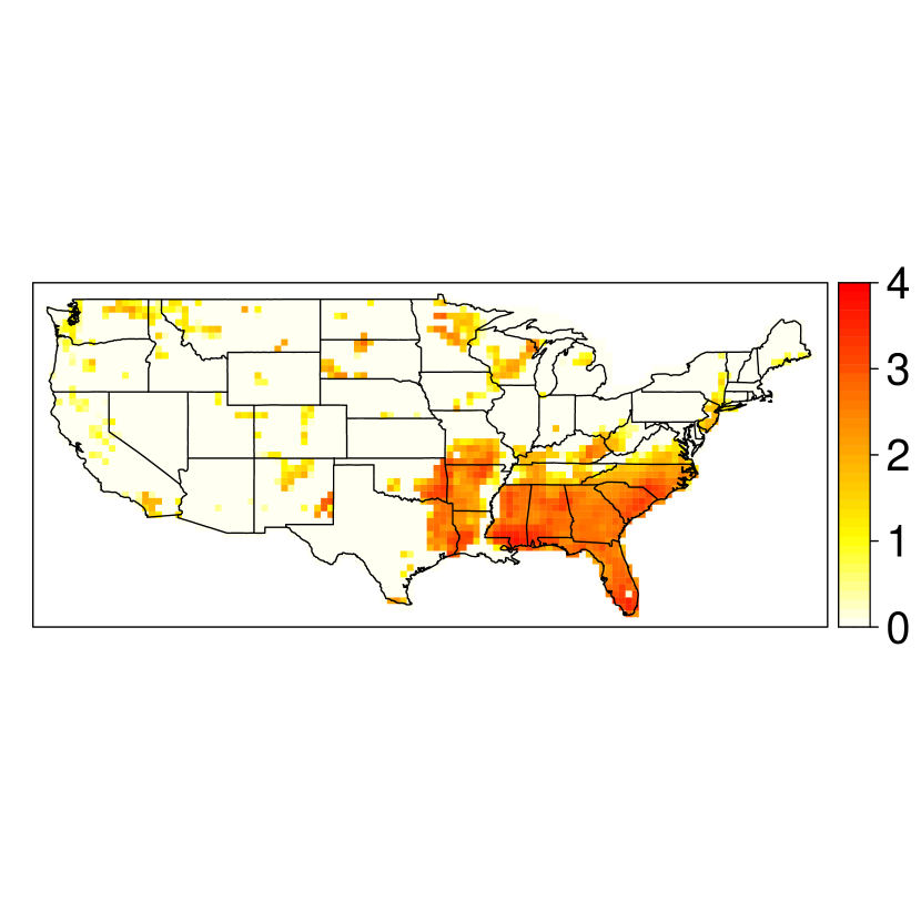
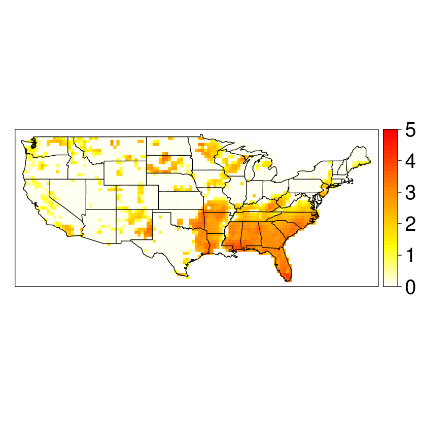
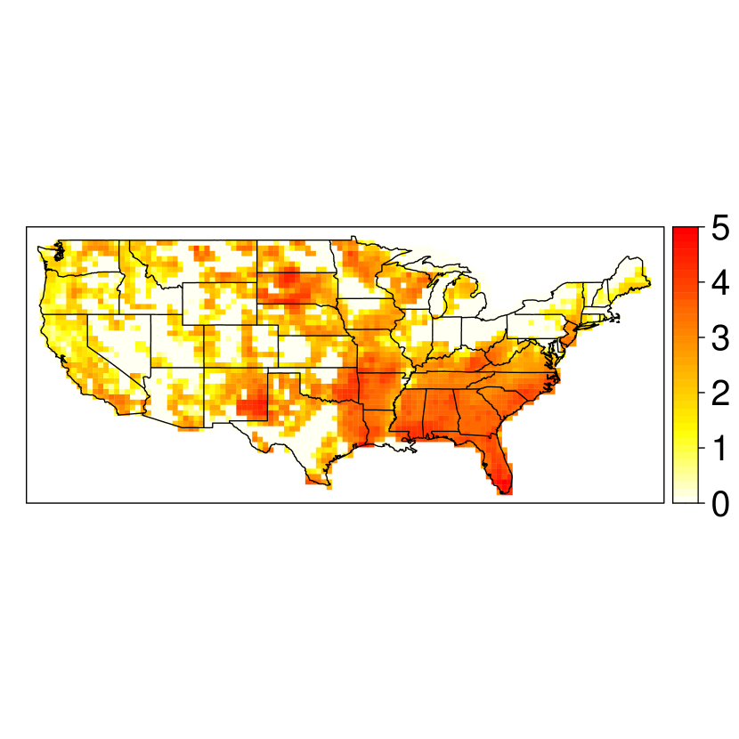
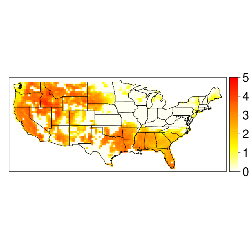
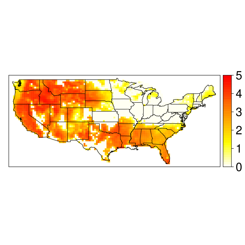
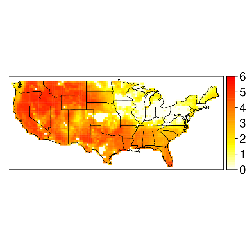
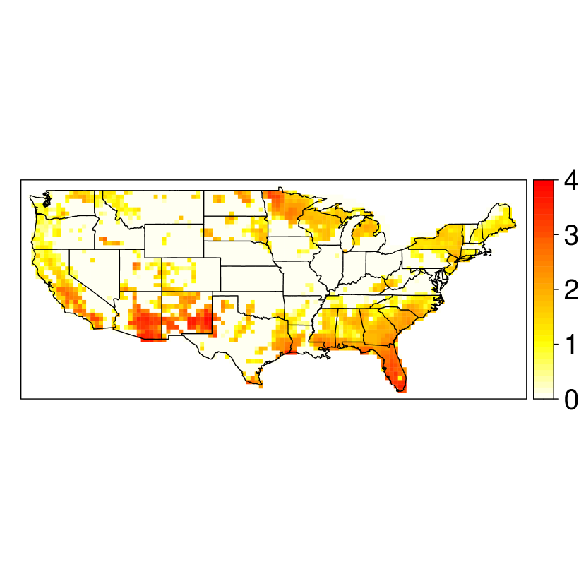
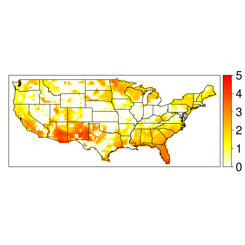
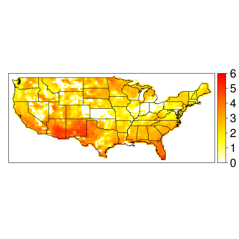
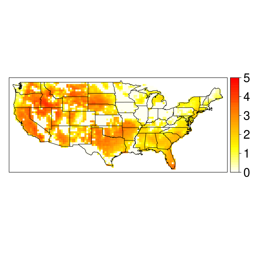
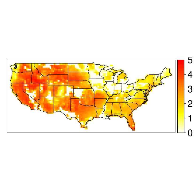
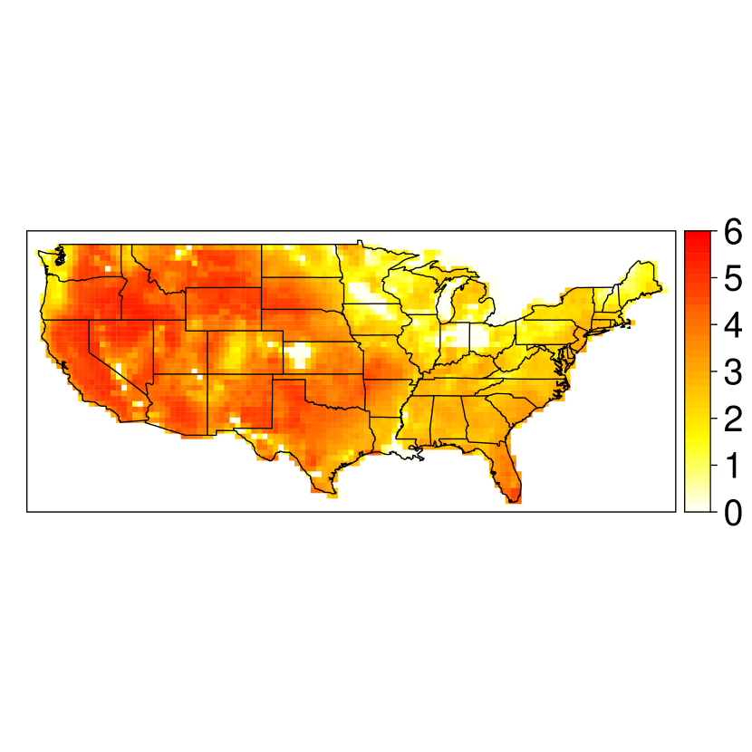
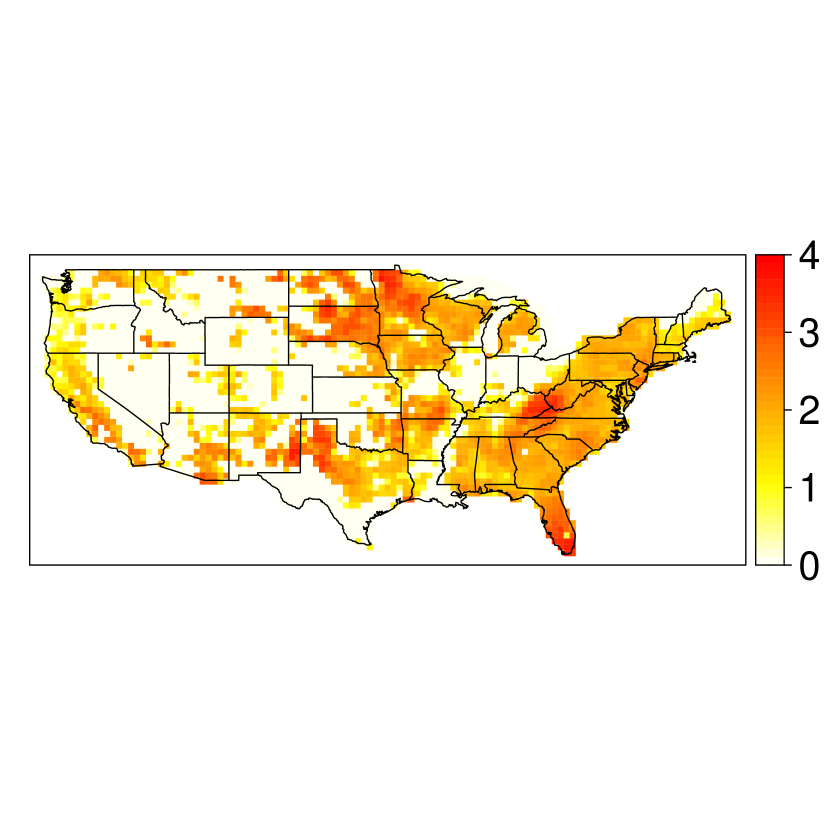
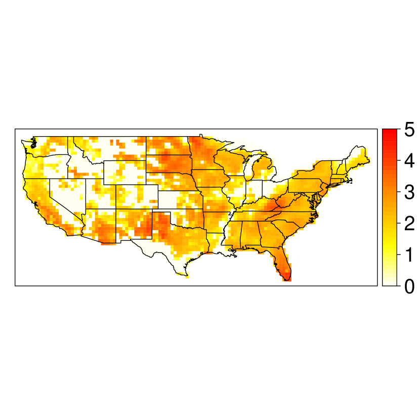
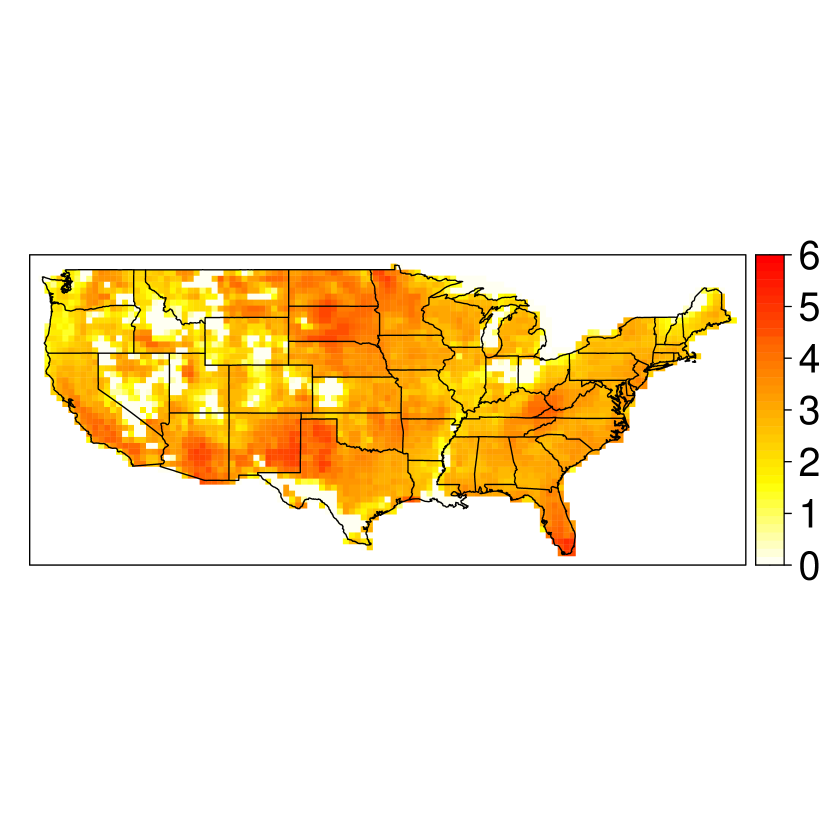
Figure S6: Maps of median estimated quantiles for $\log(1+Y(s,t))\mid\mathbf{X}(s,t)$ for different times $t$ (by row). Times, top to bottom row: March 1993, August 2000, May 2003, July 2012, April 2015. Quantiles, left to right: $90\%$, $95\%$ and $99\%$.

References

- Abatzoglou et al. (2018) Abatzoglou, J. T., Balch, J. K., Bradley, B. A. and Kolden, C. A. (2018) Human-related ignitions concurrent with high winds promote large wildfires across the USA. International journal of wildland fire 27(6), 377–386.
- Allaire and Chollet (2021) Allaire, J. and Chollet, F. (2021) keras: R Interface to ’Keras’. R package version 2.7.0.
- Allouche et al. (2021) Allouche, M., Girard, S. and Gobet, E. (2021) Tail-GAN: Simulation of extreme events with ReLu neural networks. preprint, hal:03250663.
- Barbounis et al. (2006) Barbounis, T. G., Theocharis, J. B., Alexiadis, M. C. and Dokopoulos, P. S. (2006) Long-term wind speed and power forecasting using local recurrent neural network models. IEEE Transactions on Energy Conversion 21(1), 273–284.
- Bau et al. (2017) Bau, D., Zhou, B., Khosla, A., Oliva, A. and Torralba, A. (2017) Network dissection: Quantifying interpretability of deep visual representations. In Proceedings of the IEEE Conference on Computer Vision and Pattern Recognition, pp. 6541–6549.
- Bennett et al. (2015) Bennett, K. E., Cannon, A. J. and Hinzman, L. (2015) Historical trends and extremes in boreal Alaska river basins. Journal of hydrology 527, 590–607.
- Biancofiore et al. (2015) Biancofiore, F., Verdecchia, M., Di Carlo, P., Tomassetti, B., Aruffo, E., Busilacchio, M., Bianco, S., Di Tommaso, S. and Colangeli, C. (2015) Analysis of surface ozone using a recurrent neural network. Science of the Total Environment 514, 379–387.
- Boulaguiem et al. (2022) Boulaguiem, Y., Zscheischler, J., Vignotto, E., van der Wiel, K. and Engelke, S. (2022) Modeling and simulating spatial extremes by combining extreme value theory with generative adversarial networks. Environmental Data Science 1, e5.
- Cannon (2010) Cannon, A. J. (2010) A flexible nonlinear modelling framework for nonstationary generalized extreme value analysis in hydroclimatology. Hydrological Processes: An International Journal 24(6), 673–685.
- Cannon (2011) Cannon, A. J. (2011) GEVcdn: an R package for nonstationary extreme value analysis by generalized extreme value conditional density estimation network. Computers & Geosciences 37(9), 1532–1533.
- Cannon (2018) Cannon, A. J. (2018) Non-crossing nonlinear regression quantiles by monotone composite quantile regression neural network, with application to rainfall extremes. Stochastic Environmental Research and Risk Assessment 32(11), 3207–3225.
- Carreau and Bengio (2007) Carreau, J. and Bengio, Y. (2007) A hybrid Pareto model for conditional density estimation of asymmetric fat-tail data. In Artificial Intelligence and Statistics, pp. 51–58.
- Carreau and Vrac (2011) Carreau, J. and Vrac, M. (2011) Stochastic downscaling of precipitation with neural network conditional mixture models. Water Resources Research 47(10), W10502.
- Casson and Coles (1999) Casson, E. and Coles, S. (1999) Spatial regression models for extremes. Extremes 1(4), 449–468.
- Castro-Camilo et al. (2019) Castro-Camilo, D., Huser, R. and Rue, H. (2019) A spliced gamma-generalized Pareto model for short-term extreme wind speed probabilistic forecasting. Journal of Agricultural, Biological and Environmental Statistics 24(3), 517–534.
- Castro-Camilo et al. (2022) Castro-Camilo, D., Huser, R. and Rue, H. (2022) Practical strategies for generalized extreme value-based regression models for extremes. Environmetrics p. e2742.
- Ceresetti et al. (2012) Ceresetti, D., Ursu, E., Carreau, J., Anquetin, S., Creutin, J.-D., Gardes, L., Girard, S. and Molinie, G. (2012) Evaluation of classical spatial-analysis schemes of extreme rainfall. Natural Hazards and Earth System Sciences 12(11), 3229–3240.
- Chautru (2015) Chautru, E. (2015) Dimension reduction in multivariate extreme value analysis. Electronic Journal of Statistics 9(1), 383–418.
- Chavez-Demoulin and Davison (2005) Chavez-Demoulin, V. and Davison, A. C. (2005) Generalized additive modelling of sample extremes. Journal of the Royal Statistical Society: Series C (Applied Statistics) 54(1), 207–222.
- Cho et al. (2014) Cho, K., Van Merriënboer, B., Bahdanau, D. and Bengio, Y. (2014) On the properties of neural machine translation: Encoder-decoder approaches. arXiv preprint arXiv:1409.1259.
- Cisneros et al. (2021) Cisneros, D., Gong, Y., Yadav, R., Hazra, A. and Huser, R. (2021) A combined statistical and machine learning approach for spatial prediction of extreme wildfire frequencies and sizes. arXiv preprint arXiv:2112.14920.
- Clifton et al. (2014) Clifton, D. A., Clifton, L., Hugueny, S. and Tarassenko, L. (2014) Extending the generalised Pareto distribution for novelty detection in high-dimensional spaces. Journal of Signal Processing Systems 74(3), 323–339.
- Coles (2001) Coles, S. (2001) An Introduction to Statistical Modeling of Extreme Values. Volume 208. Springer.
- Cooley et al. (2007) Cooley, D., Nychka, D. and Naveau, P. (2007) Bayesian spatial modeling of extreme precipitation return levels. Journal of the American Statistical Association 102(479), 824–840.
- Cooley and Thibaud (2019) Cooley, D. and Thibaud, E. (2019) Decompositions of dependence for high-dimensional extremes. Biometrika 106(3), 587–604.
- Copernicus (2021) Copernicus (2021) Wildfires wreaked havoc in 2021, CAMS tracked their impact. Accessed 10/02/2022. https://atmosphere.copernicus.eu/wildfires-wreaked-havoc-2021-cams-tracked-their-impact.
- D’Arcy et al. (2021) D’Arcy, E., Murphy-Barltrop, C. J. R., Shooter, R. and Simpson, E. S. (2021) A flexible, semi-parametric, cluster-based approach for predicting wildfire extremes across the contiguous United States. arXiv preprint arXiv:2112.15372.
- Davison and Huser (2015) Davison, A. C. and Huser, R. (2015) Statistics of extremes. Annual Review of Statistics and its Application 2, 203–235.
- Davison et al. (2012) Davison, A. C., Padoan, S. A. and Ribatet, M. (2012) Statistical modeling of spatial extremes. Statistical Science 27(2), 161–186.
- Dey and Salem (2017) Dey, R. and Salem, F. M. (2017) Gate-variants of gated recurrent unit (GRU) neural networks. In 2017 IEEE 60th international midwest symposium on circuits and systems (MWSCAS), pp. 1597–1600.
- Drees and Sabourin (2021) Drees, H. and Sabourin, A. (2021) Principal component analysis for multivariate extremes. Electronic Journal of Statistics 15(1), 908–943.
- Driss et al. (2017) Driss, S. B., Soua, M., Kachouri, R. and Akil, M. (2017) A comparison study between MLP and convolutional neural network models for character recognition. In Real-Time Image and Video Processing 2017, volume 10223, p. 1022306.
- Eastoe (2019) Eastoe, E. F. (2019) Nonstationarity in peaks-over-threshold river flows: A regional random effects model. Environmetrics 30(5), e2560.
- Engelke and Ivanovs (2021) Engelke, S. and Ivanovs, J. (2021) Sparse structures for multivariate extremes. Annual Review of Statistics and Its Application 8, 241–270.
- Farkas et al. (2021) Farkas, S., Lopez, O. and Thomas, M. (2021) Cyber claim analysis using generalized Pareto regression trees with applications to insurance. Insurance: Mathematics and Economics 98, 92–105.
- Gallego and Ríos Insua (2022) Gallego, V. and Ríos Insua, D. (2022) Current advances in neural networks. Annual Review of Statistics and Its Application 9(1), 197–222.
- Gebrehiwot et al. (2019) Gebrehiwot, A., Hashemi-Beni, L., Thompson, G., Kordjamshidi, P. and Langan, T. E. (2019) Deep convolutional neural network for flood extent mapping using unmanned aerial vehicles data. Sensors 19(7), 1486.
- Glorot et al. (2011) Glorot, X., Bordes, A. and Bengio, Y. (2011) Deep sparse rectifier neural networks. In Proceedings of the fourteenth international conference on artificial intelligence and statistics, pp. 315–323.
- Gnecco et al. (2022) Gnecco, N., Terefe, E. M. and Engelke, S. (2022) Extremal random forests. arXiv preprint arXiv:2201.12865.
- Gneiting and Ranjan (2011) Gneiting, T. and Ranjan, R. (2011) Comparing density forecasts using threshold-and quantile-weighted scoring rules. Journal of Business & Economic Statistics 29(3), 411–422.
- Hall (2007) Hall, B. L. (2007) Precipitation associated with lightning-ignited wildfires in Arizona and New Mexico. International Journal of Wildland Fire 16(2), 242–254.
- Harilal et al. (2021) Harilal, N., Singh, M. and Bhatia, U. (2021) Augmented convolutional LSTMs for generation of high-resolution climate change projections. IEEE Access 9, 25208–25218.
- Heffernan and Tawn (2001) Heffernan, J. E. and Tawn, J. A. (2001) Extreme value analysis of a large designed experiment: A case study in bulk carrier safety. Extremes 4(4), 359–378.
- Hochreiter and Schmidhuber (1997) Hochreiter, S. and Schmidhuber, J. (1997) Long short-term memory. Neural computation 9(8), 1735–1780.
- Vilar del Hoyo et al. (2011) Vilar del Hoyo, L., Martín Isabel, M. P. and Martínez Vega, F. J. (2011) Logistic regression models for human-caused wildfire risk estimation: analysing the effect of the spatial accuracy in fire occurrence data. European Journal of Forest Research 130(6), 983–996.
- Hrafnkelsson et al. (2021) Hrafnkelsson, B., Siegert, S., Huser, R., Bakka, H. and Jóhannesson, Á. V. (2021) Max-and-Smooth: a two-step approach for approximate Bayesian inference in latent Gaussian models. Bayesian Analysis 16(2), 611–638.
- Huser and Davison (2014) Huser, R. and Davison, A. (2014) Space–time modelling of extreme events. Journal of the Royal Statistical Society: Series B (Methodology) 76(2), 439–461.
- Ivek and Vlah (2022) Ivek, T. and Vlah, D. (2022) Reconstruction of incomplete wildfire data using deep generative models. arXiv preprint arXiv:2201.06153.
- Janßen and Wan (2020) Janßen, A. and Wan, P. (2020) -means clustering of extremes. Electronic Journal of Statistics 14(1), 1211–1233.
- Jonathan et al. (2014) Jonathan, P., Randell, D., Wu, Y. and Ewans, K. (2014) Return level estimation from non-stationary spatial data exhibiting multidimensional covariate effects. Ocean Engineering 88, 520–532.
- Keeley and Syphard (2021) Keeley, J. E. and Syphard, A. D. (2021) Large california wildfires: 2020 fires in historical context. Fire Ecology 17(1), 1–11.
- Kendon et al. (2014) Kendon, E. J., Roberts, N. M., Fowler, H. J., Roberts, M. J., Chan, S. C. and Senior, C. A. (2014) Heavier summer downpours with climate change revealed by weather forecast resolution model. Nature Climate Change 4(7), 570–576.
- Ketkar and Santana (2017) Ketkar, N. and Santana, E. (2017) Deep learning with Python. Volume 1. Springer.
- Kingma and Ba (2014) Kingma, D. P. and Ba, J. (2014) Adam: A method for stochastic optimization. arXiv preprint arXiv:1412.6980.
- Kipf and Welling (2016) Kipf, T. N. and Welling, M. (2016) Semi-supervised classification with graph convolutional networks. arXiv preprint arXiv:1609.02907.
- Koenker (2005) Koenker, R. (2005) Quantile Regression. Econometric Society Monographs. Cambridge University Press.
- Koh (2021) Koh, J. (2021) Gradient boosting with extreme-value theory for wildfire prediction. arXiv preprint arXiv:2110.09497.
- Koh et al. (2021) Koh, J., Pimont, F., Dupuy, J.-L. and Opitz, T. (2021) Spatiotemporal wildfire modeling through point processes with moderate and extreme marks. arXiv preprint arXiv:2105.08004.
- Lenzi et al. (2021) Lenzi, A., Bessac, J., Rudi, J. and Stein, M. L. (2021) Neural networks for parameter estimation in intractable models. arXiv preprint arXiv:2107.14346.
- Li et al. (2015) Li, Y., Tarlow, D., Brockschmidt, M. and Zemel, R. (2015) Gated graph sequence neural networks. arXiv preprint arXiv:1511.05493.
- Liu et al. (2018a) Liu, J., Zhang, T., Han, G. and Gou, Y. (2018a) TD-LSTM: Temporal dependence-based LSTM networks for marine temperature prediction. Sensors 18(11), 3797.
- Liu et al. (2018b) Liu, L., Han, M., Zhou, Y. and Wang, Y. (2018b) LSTM recurrent neural networks for influenza trends prediction. In International Symposium on Bioinformatics Research and Applications, pp. 259–264.
- Mannshardt-Shamseldin et al. (2010) Mannshardt-Shamseldin, E. C., Smith, R. L., Sain, S. R., Mearns, L. O. and Cooley, D. (2010) Downscaling extremes: A comparison of extreme value distributions in point-source and gridded precipitation data. The Annals of Applied Statistics 4, 484–502.
- Medina et al. (2017) Medina, E., Petraglia, M. R., Gomes, J. G. R. and Petraglia, A. (2017) Comparison of CNN and MLP classifiers for algae detection in underwater pipelines. In 2017 Seventh International Conference on Image Processing Theory, Tools and Applications (IPTA), pp. 1–6.
- Mitchell (2013) Mitchell, J. W. (2013) Power line failures and catastrophic wildfires under extreme weather conditions. Engineering Failure Analysis 35, 726–735.
- Naveau et al. (2016) Naveau, P., Huser, R., Ribereau, P. and Hannart, A. (2016) Modeling jointly low, moderate, and heavy rainfall intensities without a threshold selection. Water Resources Research 52(4), 2753–2769.
- Opitz (2022) Opitz, T. (2022) Editorial: EVA 2021 Data Competition on spatio-temporal prediction of wildfire activity in the United States. Extremes (to appear) .
- Opitz et al. (2018) Opitz, T., Huser, R., Bakka, H. and Rue, H. (2018) INLA goes extreme: Bayesian tail regression for the estimation of high spatio-temporal quantiles. Extremes 21(3), 441–462.
- Papastathopoulos and Tawn (2013) Papastathopoulos, I. and Tawn, J. A. (2013) Extended generalised Pareto models for tail estimation. Journal of Statistical Planning and Inference 143(1), 131–143.
- Pereira and Turkman (2019) Pereira, J. and Turkman, K. (2019) Statistical models of vegetation fires: Spatial and temporal patterns. In Handbook of Environmental and Ecological Statistics, pp. 401–420. CRC Press.
- Politis and Romano (1994) Politis, D. N. and Romano, J. P. (1994) The stationary bootstrap. Journal of the American Statistical Association 89(428), 1303–1313.
- Ramachandran et al. (2017) Ramachandran, P., Zoph, B. and Le, Q. V. (2017) Searching for activation functions. arXiv preprint arXiv:1710.05941.
- Richards (2022) Richards, J. (2022) pinnEV: Partially-Interpretable Neural Networks for modelling of Extreme Values. R package.
- Richards et al. (2022) Richards, J., Tawn, J. A. and Brown, S. J. (2022) Joint estimation of extreme spatially aggregated precipitation at different scales through mixture modelling. arXiv preprint arXiv:2111.08469.
- Rietsch et al. (2013) Rietsch, T., Naveau, P., Gilardi, N. and Guillou, A. (2013) Network design for heavy rainfall analysis. Journal of Geophysical Research: Atmospheres 118(23), 13–075.
- Rodrigues and Pereira (2020) Rodrigues, F. and Pereira, F. C. (2020) Beyond expectation: Deep joint mean and quantile regression for spatiotemporal problems. IEEE Transactions on Neural Networks and Learning Systems 31(12), 5377–5389.
- Rodrigues and de la Riva (2014) Rodrigues, M. and de la Riva, J. (2014) An insight into machine-learning algorithms to model human-caused wildfire occurrence. Environmental Modelling & Software 57, 192–201.
- Rothfuss et al. (2019) Rothfuss, J., Ferreira, F., Walther, S. and Ulrich, M. (2019) Conditional density estimation with neural networks: Best practices and benchmarks. arXiv preprint arXiv:1903.00954.
- Rudd et al. (2017) Rudd, E. M., Jain, L. P., Scheirer, W. J. and Boult, T. E. (2017) The extreme value machine. IEEE transactions on Pattern Analysis and Machine Intelligence 40(3), 762–768.
- Samek et al. (2021) Samek, W., Montavon, G., Lapuschkin, S., Anders, C. J. and Müller, K.-R. (2021) Explaining deep neural networks and beyond: A review of methods and applications. Proceedings of the IEEE 109(3), 247–278.
- Sang and Gelfand (2010) Sang, H. and Gelfand, A. E. (2010) Continuous spatial process models for spatial extreme values. Journal of Agricultural, Biological, and Environmental Statistics 15(1), 49–65.
- Scarselli et al. (2008) Scarselli, F., Gori, M., Tsoi, A. C., Hagenbuchner, M. and Monfardini, G. (2008) The graph neural network model. IEEE Transactions on Neural Networks 20(1), 61–80.
- Short (2017) Short, K. C. (2017) Spatial wildfire occurrence data for the United States, 1992-2015 [FPA_FOD_20170508]. 4th Ed. Fort Collins, CO: Forest Service Research Data Archive.
- Shrestha et al. (2017) Shrestha, R. R., Cannon, A. J., Schnorbus, M. A. and Zwiers, F. W. (2017) Projecting future nonstationary extreme streamflow for the Fraser River, Canada. Climatic Change 145(3), 289–303.
- Shuofeng et al. (2021) Shuofeng, L., Puwen, L. and Koyamada, K. (2021) LSTM based hybrid method for basin water level prediction by using precipitation data. Journal of Advanced Simulation in Science and Engineering 8(1), 40–52.
- Silverman (1985) Silverman, B. W. (1985) Some aspects of the spline smoothing approach to non-parametric regression curve fitting. Journal of the Royal Statistical Society: Series B (Methodology) 47(1), 1–21.
- Smith et al. (2020) Smith, A., Jones, M., Abatzoglou, J., Canadell, J. and Betts, R. (2020) Sciencebrief review: Climate change increases the risk of wildfires. In: Critical Issues in Climate Change Science, edited by: C. Le Quéré, P. Liss, P. Forster. https://doi.org/10.5281/zenodo.4570195.
- Smith (1985) Smith, R. L. (1985) Maximum likelihood estimation in a class of nonregular cases. Biometrika 72(1), 67–90.
- Smith (1989) Smith, R. L. (1989) Extreme value analysis of environmental time series: An application to trend detection in ground-level ozone. Statistical Science 4(4), 367 – 377.
- Vandeskog et al. (2021) Vandeskog, S. M., Martino, S., Castro-Camilo, D. and Rue, H. (2021) Modelling short-term precipitation extremes with the blended generalised extreme value distribution. arXiv preprint arXiv:2105.09062.
- Vasiliades et al. (2015) Vasiliades, L., Galiatsatou, P. and Loukas, A. (2015) Nonstationary frequency analysis of annual maximum rainfall using climate covariates. Water Resources Management 29(2), 339–358.
- Velthoen et al. (2021) Velthoen, J., Dombry, C., Cai, J.-J. and Engelke, S. (2021) Gradient boosting for extreme quantile regression. arXiv preprint arXiv:2103.00808.
- Vignotto and Engelke (2020) Vignotto, E. and Engelke, S. (2020) Extreme value theory for anomaly detection–the GPD classifier. Extremes 23(4), 501–520.
- Wood (2006) Wood, S. (2006) Generalized Additive Models: An Introduction with R. Chapman & Hall/CRC Texts in Statistical Science. Taylor & Francis.
- Wood (2003) Wood, S. N. (2003) Thin plate regression splines. Journal of the Royal Statistical Society: Series B (Methodology) 65(1), 95–114.
- Yadav et al. (2021) Yadav, R., Huser, R. and Opitz, T. (2021) Spatial hierarchical modeling of threshold exceedances using rate mixtures. Environmetrics 32(3), e2662.
- Yamashita et al. (2018) Yamashita, R., Nishio, M., Do, R. K. G. and Togashi, K. (2018) Convolutional neural networks: an overview and application in radiology. Insights into imaging 9(4), 611–629.
- Youngman (2019) Youngman, B. D. (2019) Generalized additive models for exceedances of high thresholds with an application to return level estimation for US wind gusts. Journal of the American Statistical Association 114(528), 1865–1879.
- Yu et al. (2020) Yu, Y., Han, X., Yang, M. and Yang, J. (2020) Probabilistic prediction of regional wind power based on spatiotemporal quantile regression. IEEE Transactions on Industry Applications 56(6), 6117–6127.
- Yuan et al. (2019) Yuan, S., Luo, X., Mu, B., Li, J. and Dai, G. (2019) Prediction of North Atlantic Oscillation index with convolutional LSTM based on ensemble empirical mode decomposition. Atmosphere 10(5), 252.
- Zanini et al. (2020) Zanini, E., Eastoe, E., Jones, M., Randell, D. and Jonathan, P. (2020) Flexible covariate representations for extremes. Environmetrics 31(5), e2624.
- Zhang et al. (2019) Zhang, G., Wang, M. and Liu, K. (2019) Forest fire susceptibility modeling using a convolutional neural network for Yunnan province of China. International Journal of Disaster Risk Science 10(3), 386–403.
- Zhang and Zhu (2018) Zhang, Q. and Zhu, S.-C. (2018) Visual interpretability for deep learning: a survey.
- Zhang et al. (2022) Zhang, Z., Krainski, E., Zhong, P., Rue, H. and Huser, R. (2022) Joint modeling and prediction of massive spatio-temporal wildfire count and burnt area data with the INLA-SPDE approach. arXiv preprint arXiv:2202.06502.
- Zhong et al. (2022) Zhong, P., Huser, R. and Opitz, T. (2022) Modeling nonstationary temperature maxima based on extremal dependence changing with event magnitude. The Annals of Applied Statistics 16(1), 272–299.
- Zhong and Wang (2021) Zhong, Q. and Wang, J.-L. (2021) Neural networks for partially linear quantile regression. arXiv preprint arXiv:2106.06225.
- Zhou et al. (2020) Zhou, J., Cui, G., Hu, S., Zhang, Z., Yang, C., Liu, Z., Wang, L., Li, C. and Sun, M. (2020) Graph neural networks: A review of methods and applications. AI Open 1, 57–81.