Bucketized Active Sampling for Learning ACOPF

Abstract

This paper considers optimization proxies for Optimal Power Flow (OPF), i.e., machine-learning models that approximate the input/output relationship of OPF. Recent work has focused on showing that such proxies can be of high fidelity. However, their training requires significant data, each instance necessitating the (offline) solving of an OPF for a sample of the input distribution. To meet the requirements of market-clearing applications, this paper proposes Bucketized Active Sampling (BAS), a novel active learning framework that aims at training the best possible OPF proxy within a time limit. BAS partitions the input distribution into buckets and uses an acquisition function to determine where to sample next. By applying the same partitioning to the validation set, BAS leverages labeled validation samples in the selection of unlabeled samples. BAS also relies on an adaptive learning rate that increases and decreases over time. Experimental results demonstrate the benefits of BAS.

This research was partly supported by NSF award 2112533 and ARPA-E PERFORM award AR0001136.

I Introduction

The AC Optimal Power Flow (ACOPF) is a core building block in power systems that finds the most economical generation dispatch meeting the load demand, while satisfying the physical and operational constraints of the underlying systems. The problem is used in many applications including day-ahead security-constrained unit commitment (SCUC) [1], real time security-constrained economic dispatch (SCED) [2], and expansion planning [3].

The non-convexity of ACOPF limits the solving frequency of many operational tools. In practice, generation schedules in real time markets are required to be updated every 5 – 15 minutes, varying from region to region. With the continuous integration of renewable energy sources and demand response mechanisms to meet renewable targets, load and generation uncertainties are expected to be more and more severe. Solving generation schedules using historical forecasts may no longer be optimal, and may not even be feasible in the worst case. Balancing generation and load rapidly without sacrificing economical efficiency is thus an important challenge.

Recently, an interesting line of research has focused on how to learn and predict ACOPF using optimization proxies, such as Deep Neural Networks (DNN) [4, 5, 6]. Once a DNN model is trained, predictions can be computed in milliseconds. Preliminary results are encouraging, indicating that DNNs can predict ACOPF solutions with high accuracy. However, most prior work [7, 8, 9, 10, 6, 11, 12, 13, 14] ignore the computational time spent gathering or sampling ACOPF training data in practice. In particular, when generator commitments and grid topology change from day to day (or even within hours) e.g. to respond to wind forecast updates, it becomes impractical to develop a sophisticated learning mechanism that requires hours to sample and solve ACOPF instances. On the other hand, generating data sets and training a generalized framework “once-for-all” for all possible commitments, forecasts, and potential grid topologies is also unlikely to be feasible due to the exponential number of configurations & scenarios of a transmission grid. Therefore, how to actively generate samples and train a “Just-in-Time” model [15], based on the current and forecasted information, is an important practical question for learning approaches.

This paper is the first to study whether active sampling can address this important issue and, more generally, aims at decreasing the computational resources needed to train optimization proxies in practice. It proposes Bucketized Active Sampling (BAS), a novel active learning framework to perform “Just-in-Time” (JIT) training. Unlike many active learning frameworks that generate new samples based on the evaluations of individual (or groups of [16]) unlabeled data samples, BAS reasons about regions of the input distribution, exploiting the fact that similar inputs should generally produce similar outputs. The input distribution is thus bucketized and each bucket is evaluated (using an independent validation set) to determine if it needs additional samples. A variety of acquisition functions are examined, some inspired by several state-of-the-art approaches, e.g., BADGE [17], and MCDUE [18]. BAS is evaluated on large transmission networks and compared to the state of the art in active sampling. The experimental results show that BAS produces significant benefits for JIT training. This paper’s contributions can thus be summarized as follows:

1. The paper proposes BAS, a novel bucketized active learning framework for the Just-In-Time learning setting. Its key novelty is the idea of partitioning the input distribution into buckets to determine which buckets are in need of additional samples. This bucket-based sampling contrasts with existing active learning schemes that determine which unlabeled samples to add based on the evaluation of their individual properties.

2. To determine which buckets are in need of more samples, BAS bucketizes the validation set in order to score each region of the input distribution, decoupling the assessment of where new samples are needed from the sample generation. This allows additional flexibility when learning optimization proxies, including the ability to avoid generating too many infeasible problems.

3. The paper studies multiple acquisition functions for BAS, highlighting the benefits of gradient information.

4. The paper proposes a new dynamic adjustment scheme for the learning rate that may now decrease and increase.

5. The paper presents an experimental evaluation of BAS on large ACOPF benchmarks, demonstrating its benefits compared to state-of-the-art approaches.

The rest of the paper is organized as follows. Section II presents background materials on ACOPF and active sampling. Section III discusses related work on active sampling and ACOPF learning. Section IV introduces the novel active sampling framework. Section V reports experimental evaluations and Section VI concludes the paper.

II Background

This paper uses calligraphic capitals $\mathcal{X}$ for sets and gothic capitals $\mathfrak{X}$ for distributions. The complex conjugate of $z\,{\in}\,\mathbb{C}$ is denoted $z^{\star}$. For decision variable $y$, its lower and upper bounds are denoted by $\overline{y}$ and $\underline{y}$, optimal value by $y^{*}$, and predicted value by $\hat{y}$. $\mathbf{x}$ and $\mathbf{y}$ represent the (flattened) vector of input and output features, respectively.

II-A AC Optimal Power Flow

The AC Optimal Power Flow (ACOPF) aims at finding the most economical generation dispatch to meet load demand, while satisfying both the transmission and operational constraints. The ACOPF problem is nonlinear and non-convex.

Model 1 AC Optimal Power Flow — ACOPF($\mathbf{S}^{\text{d}}$)

$$\min\quad \sum_{i\in\mathcal{N}}c_{i}(\mathbf{S}^{\text{g}}_{i})$$ (1a)

s.t. $$\mathbf{S}^{\text{g}}_{i}-\mathbf{S}^{\text{d}}_{i}=\sum_{(i,j)\in\mathcal{E}_{i}\cup\mathcal{E}^{R}_{i}}\mathbf{S}^{\text{f}}_{ij} \forall i\in\mathcal{N}$$ (1b)

$$\mathbf{S}^{\text{f}}_{ij}=(Y_{ij}+Y^{c}_{ij})^{\star}\mathbf{V}_{i}\mathbf{V}_{i}^{\star}-Y_{ij}^{\star}\mathbf{V}_{i}\mathbf{V}_{j}^{\star} \forall(i,\,j)\in\mathcal{E}$$ (1c)

$$\mathbf{S}^{\text{f}}_{ji}=(Y_{ij}+Y^{c}_{ji})^{\star}\mathbf{V}_{j}\mathbf{V}_{j}^{\star}-Y_{ij}^{\star}\mathbf{V}_{i}^{\star}\mathbf{V}_{j} \forall(i,\,j)\in\mathcal{E}$$ (1d)

$$\underline{\mathbf{v}_{i}}\leq|\mathbf{V}_{i}|\leq\overline{\mathbf{v}_{i}} \forall i\in\mathcal{N}$$ (1e)

$$\underline{\mathbf{S}^{\text{g}}_{i}}\leq\mathbf{S}^{\text{g}}_{i}\leq\overline{\mathbf{S}^{\text{g}}_{i}} \forall i\in\mathcal{N}$$ (1f)

$$|\mathbf{S}^{\text{f}}_{ij}|,|\mathbf{S}^{\text{f}}_{ji}|\leq\overline{S_{ij}}^{2} \forall(i,\,j)\in\mathcal{E}$$ (1g)

Let $\mathcal{P}\,{=}\,\{\mathcal{N},\,\mathcal{L},\,\mathcal{G},\,\mathcal{E}\}$ be a power grid with buses $\mathcal{N}$, loads $\mathcal{L}$, generators $\mathcal{G}$, and transmission branches (lines and transformers) $\mathcal{E}$. For each bus $i\,{\in}\,\mathcal{N}$, define $\mathcal{E}_{i}\,{=}\,\{(i,\,j)\,{\in}\,\mathcal{E}\}$ and $\mathcal{E}^{R}_{i}\,{=}\,\{(i,\,j)\,{\in}\,\mathcal{E}^{R}\}$ where $\mathcal{E}^{R}\,{=}\,\{(j,\,i)\,|\,(i,\,j)\in\mathcal{E}\}$. For ease of presentation, the paper assumes that exactly one generator and one load is attached to each bus. The ACOPF problem is formulated in Model 1, where $\mathbf{V}$ denotes complex voltage, and $\mathbf{S}^{\text{d}},\mathbf{S}^{\text{g}},\mathbf{S}^{\text{f}}$ denote complex power demand, generation and flow, respectively. The line and shunt admittance of branch $(i,\,j)$ are denoted by $Y_{ij}$ and $Y^{c}_{ij}$. Objective (1a) minimizes total generation costs. Constraints (1b) maintain power balance (Kirchkoff’s current law) for all the buses. Constraints (1c), (1d) assert Ohm’s Law for all the lines. Constraint (1e) enforces upper and lower bounds for voltage magnitude $|\mathbf{V}|$. Constraints (1f) impose bounds on active and reactive generation. Constraint (1g) enforces the thermal limits $\overline{S_{ij}}$ on the apparent power for each line. For simplicity, Model 1 omits the detailed equations for bus shunts and transformers. These components are considered and implemented in this work.

II-B Sampling for OPF proxies

Training optimization proxies for OPF requires generating a dataset of OPF instances and their solutions. This is done by sampling OPF instances according to a pre-specified distribution, then solving each sampled instance to obtain its solution.

Algorithm 1 ACOPF Load Perturbation (LoadPerturb)

1:Input: Nominal sample $\mathbf{S}^{\text{d}}_{0}$, regional load variation distribution $\mathfrak{B}$, individual noise variation distribution $\mathfrak{E}$, and data set size $n$.

2:$\mathcal{D}\leftarrow\{\}$

3:for $i=1\dots n$ do

4:     $b_{i}\sim\mathfrak{B}$

5:     $\bm{\epsilon}_{i}\sim\mathfrak{E}$

6:     $\mathbf{x}_{i}\leftarrow b_{i}\cdot\mathbf{S}^{\text{d}}_{0}\circ\bm{\epsilon}_{i}$

7:     $\mathbf{y}_{i}~{}\leftarrow~{}(\mathbf{S}^{\text{g}},\,\mathbf{V})\leftarrow\texttt{{ACOPF}{}}(\mathbf{x}_{i})$

8:     if $\mathbf{y}_{i}$ has been successfully found then

9:         $\mathcal{D}\leftarrow\mathcal{D}\cup\{(\mathbf{x}_{i},\mathbf{y}_{i})\}$

10:     end if

11:end for

12:return $\mathcal{D}$

Algorithm 1 shows a random sampling procedure that perturbs load values from a nominal point $\mathbf{x}_{0}$. The algorithm considers both regional influence and individual variations, modeled by the two variation distributions $\mathfrak{B}$ and $\mathfrak{E}$. This general data generation pipeline is common among prior work, e.g., [6, 13, 14, 9, 10, 11, 12], though not all prior approaches consider both regional and individual variations and not all prior approaches predict all the solution variables for ACOPF.

II-C Active Sampling

Active sampling [19, 20, 21, 22] aims at finding a small set $\mathcal{D}$ of data samples from a distribution $\mathfrak{D}_{U}$ to train a machine-learning model. In other words, given an unlabeled sample distribution $\mathfrak{D}_{U}$, the goal of active sampling is to design a query strategy $Q$ that chooses a small set of samples $\mathcal{D}$ from $\mathfrak{D}_{U}$ to label. Let $\mathbf{x}$ and $\mathbf{y}$ be the vector of input and output features of a data sample, i.e., $(\mathbf{x},\,\mathbf{y})\in\mathcal{D}$, $h$ be a learning model, i.e., $h(\mathbf{x})=\hat{\mathbf{y}}$, and $\mathbb{L}$ be a loss metric for measuring the prediction quality. The data set $\mathcal{D}^{*}$ with the highest prediction accuracy is defined by a bilevel optimization problem:

$$\mathcal{D}^{*}\in\operatorname*{\text{argmin}}_{\mathcal{D}} \enspace\operatorname*{\mathbb{E}}_{(\mathbf{x},\,\mathbf{y})\sim\mathfrak{D}}\left[\mathbb{L}(h_{\mathcal{D}}^{*}(\mathbf{x}),\,\mathbf{y})\right]$$ (2a)

s.t. $$\quad h_{\mathcal{D}}^{*}\in\operatorname*{\text{argmin}}_{h}\sum_{(\mathbf{x},\,\mathbf{y})\in\mathcal{D}}\mathbb{L}(h(\mathbf{x}),\,\mathbf{y})$$ (2b)

Solving (2) optimally is challenging. For many applications, drawing samples incrementally during training is more computationally efficient. Let $\mathcal{D}^{S}=\operatorname{\text{supp}}(\mathfrak{D}_{U})$ be the support set of distribution $\mathfrak{D}_{U}$. Acquisition functions $\alpha$ (or scoring functions [23]) are commonly used in active sampling applications to select the best $k$ samples from $\mathcal{D}^{S}$ for the next training cycle. The set $\mathcal{D}^{*}_{k}$ containing the $k$ best samples drawn with acquisition function $\alpha$ is defined as:

$$\mathcal{D}^{*}_{k}\in\operatorname*{\text{argmax}}_{\mathcal{D}_{k}\subseteq\mathcal{D}^{S}\mbox{ s.t. }|\mathcal{D}_{k}|=k}\enspace\alpha\left(\mathcal{D}_{k}\right)$$ (3)

Note that acquisition functions are usually customized per application. Many acquisition functions analyze/query the learning model $h$ to select the next set $\mathcal{D}^{*}_{k}$ for training.

III Related Work

Most general active learning / sampling mechanisms [24, 18, 25] label data samples based on acquisition scores of individual samples. Scores are often computed based on evaluations of the learning model, and the subset of samples with the highest scores will then be added to the data set. Some work also considers correlations between candidate input samples and/or ranking multiple unlabeled samples at the same time as a batch, e.g., BatchBALD [16] and BADGE [17].

Contrary to prior approaches, BAS does not work at the level of individual samples: instead, it partitions the input distribution in various regions and determines, based on a dedicated validation set, which regions are in need of more samples. The validation set contains a list of buckets, where each bucket contains labeled validation samples for each individual partitioned subspace. BAS has several advantages: it exploits the structure of the underlying distribution, and it separates the analysis of the regions from the sampling process. In the context of optimization proxies, BAS also makes it possible to avoid generating infeasible inputs.

The effects of increasing learning rate during training have been the focus of several recent works including [26, 27, 28, 29]. However, prior active learning approaches focus only on decreasing the learning rate during training [30, 31]. One of the novelties of the proposed scheme is to also increase the learning rate when appropriate, avoiding premature termination.

IV Active Learning for ACOPF

This section describes the novel active learning framework BAS. It first presents the Deep Neural Network (DNN) for ACOPF learning. It then introduces the core idea of BAS before going into the individual components in detail.

IV-A Active Learning: DNN Model

The ACOPF problem in Model 1 can be viewed as a high dimensional nonlinear function $h_{\mbox{ac}}$, taking input vector $\mathbf{S}^{\text{d}}$, and returning optimal values for $\mathbf{S}^{\text{g}}$ and $\mathbf{V}$. The learning task for OPF typically generates a finite set $\mathcal{D}$ of data samples, and each sample $(\mathbf{x},\,\mathbf{y})\in\mathcal{D}$ is of the form: $\mathbf{x}=(\mathbf{S}^{\text{d}}),\enspace\mathbf{y}=(\mathbf{S}^{\text{g}},\,\mathbf{V}).$ Subscripts on $\mathbf{x}/\mathbf{y}$ identify particular samples, e.g., $\mathbf{x}_{i}$ refers to the input features of the $i^{\text{th}}$ sample.

This work uses Deep Neural Networks (DNNs) to illustrate the benefits of active learning for speeding up ACOPF learning. A DNN $h_{\theta}$ is composed of a sequence of $t$ layers, with each layer taking as input the results of the previous layer [32]:

$$\mathbf{h}^{0}(\mathbf{x}) =\mathbf{x}$$

$$\mathbf{h}^{j}(\mathbf{x}) =\pi(\mathbf{W}^{j}\mathbf{h}^{j-1}(\mathbf{x})+\mathbf{b}^{j}) \forall j\in[1,t]$$

where $\mathbf{x}$, $\mathbf{W}^{j}$, $\mathbf{b}^{j}$, and $\pi$ define the input vector, the $j^{\text{th}}$ weight matrix, the $j^{\text{th}}$ bias vector, and the activation function respectively. $\theta$ refers to the set of all $\mathbf{W}^{j}$ and $\mathbf{b}^{j}$ for $j\in[1,t]$. The problem of training a DNN $h_{\theta}$ on a dataset $\mathcal{D}$ consists of finding the parameters $\theta^{*}$ that minimize empirical risk:

$$\theta^{*}\in\operatorname*{\text{argmin}}_{\theta}\sum_{(\mathbf{x},\,\mathbf{y})\in\mathcal{D}}\mathbb{L}(h_{\theta}(\mathbf{x}),\,\mathbf{y})$$ (4)

IV-B The Active Learning Scheme for BAS

Algorithm 2 depicts the overall structure of the training loop. The main contributions are in the algorithm for active sampling presented in Section IV-C and Algorithm 3.

Algorithm 2 Active Learning Loop

1:Parameters: Initial learning rate $\beta_{0}$; Learning rate bounds $\overline{\beta}$ & $\underline{\beta}$; Patience thresholds $\overline{\rho_{1}}$ & $\overline{\rho_{2}}$; Learning rate factors $\gamma_{1}$ & $\gamma_{2}$; Termination condition $\textsc{ShouldStop}(\cdot)$

2:Inputs: Initial data set $\mathcal{D}_{0}$; Bucket-validation set $\mathcal{D}_{V}$; DNN $h_{\theta}$

3:Outputs: DNN $h_{\theta}$  

4:$\beta\leftarrow\beta_{0}$, $l^{*}_{V}\leftarrow\infty$, $\rho_{1}\leftarrow 0,\rho_{2}\leftarrow 0$, $\mathcal{D}\leftarrow\mathcal{D}_{0}$,

5:while $\neg\textsc{ShouldStop}(\cdot)$ do

6: ${\rhd}$ Training

7:     $h_{\theta}\leftarrow\textsc{Train}(h_{\theta},\,\mathcal{D},\,\beta)$

8: ${\rhd}$ Validation & Patience Update

9:     $l_{V}\leftarrow\displaystyle\sum_{(\mathbf{x},\mathbf{y})\in\mathcal{D}_{V}}\mathbb{L}(h_{\theta}(\mathbf{x}),\,\mathbf{y})$

10:     $\rho_{1},\,\rho_{2},\,l^{*}_{V},\,\beta\leftarrow{\textsc{Patience}}(\rho_{1},\,\rho_{2},\,l_{V},\,l^{*}_{V},\,\beta)$

11: ${\rhd}$ Active Sampling

12:     if $\rho_{2}=0$ then

13:         $\mathcal{D}\leftarrow\mathcal{D}\cup{\textsc{BAS}{}}\left(h_{\theta},\mathcal{D}_{V}\right)$

14:     end if

15:end while

The algorithm receives an initial data set $\mathcal{D}_{0}$, a validation data set $\mathcal{D}_{V}$, and an initialized DNN model $h_{\theta}$ as inputs. The initial and validation data sets $\mathcal{D}_{0}$ and $\mathcal{D}_{V}$ can be constructed from Algorithm 1 or from historically known ACOPF solutions. Let $\mathfrak{D}$ be the distribution from which the inputs are drawn. Prior to training, the input distribution $\mathfrak{D}$ is partitioned into buckets. This partitioning is applied to both $\mathfrak{D}$ and $\mathcal{D}_{V}$ to form buckets containing a (potentially infinite) set of unlabeled samples from $\mathfrak{D}$ and a finite set of corresponding labeled validation samples from $\mathcal{D}_{V}$. Note that the partitioning scheme should be such that it allows for sampling from a particular partition/bucket. Line 1 initializes the routine variables including the learning rate, best validation loss, patience counters, and training set. Lines 5-15 constitute the main loop of the training algorithm, which terminates when $\textsc{ShouldStop}(\cdot)$ is true, typically a bound on time or iterations. Line 7 updates the parameters of the DNN $h_{\theta}$ using the dataset $\mathcal{D}$ and learning rate $\beta$. Line 9 computes the validation loss using the bucket-validation set. Line 10 calls the Patience routine (Algorithm 4) to update the patience counters $\rho_{1},\,\rho_{2}$ and the learning rate $\beta$. See Section IV-D for more details on patience-based scheduling. Finally, if the patience counter $\rho_{2}$ exceeds its threshold, new samples are drawn and their ACOPF is computed (Lines 12 - 14) following BAS (Algorithm 3).

IV-C Bucketized Active Sampling

Algorithm 3 presents the active sampling routine BAS. The key innovation of BAS is that by partitioning the input distribution into regions (buckets) that capture the inherent structure of the application at hand, BAS can decouple the assessment of where additional samples are needed from the sample generation. Instead of generating samples based on their individual qualities, BAS uses a pre-chosen set (the bucket-validation set) to determine the regions where samples are most needed. By comparing properties across different buckets, BAS effectively allocates computational resources to poorly performing regions, resulting in a more efficient sampling and learning routine.

The general process is described next. Step 4 partitions the bucket-validation data set. Step 6 evaluates the buckets using the acquisition function $\alpha$ and returns a set $\mathcal{S}$ of scores $s_{i}$, reflecting the urgency that new samples needed in bucket $i$. Step 8 uses a distributor function to decide how many samples to generate for each bucket based on the scores. Step 10 generates the input feature vectors $\mathbf{x}_{j}$ by sampling from a predefined distribution $\mathfrak{D}_{B_{i}}$ for each bucket $i$. See V-B for how $\mathfrak{D}_{B_{i}}$ can be defined. Step 12 computes the ACOPF solutions and records the output $\mathbf{y}_{j}$ for each generated input $\mathbf{x}_{j}$ across all the buckets. Step 15 reconstructs the new samples and returns them to the main learning routine.

Algorithm 3 BAS: Bucketized Active Sampling

1:Parameters: Acquisition function $\alpha$; Distributor function $\eta$; Maximum number of new samples $\overline{n}$

2: Inputs: DNN $h_{\theta}$, Bucket-validation set $\mathcal{D}_{V}$

3:Output: Set of new samples $\mathcal{D}^{+}$  

4:Partition bucket-validation data into a set of $k$ buckets

5: $\{B_{1},B_{2},\dotsc,B_{k}\}\leftarrow\textsc{Partition}(\mathcal{D}_{V})$

6:Evaluate each bucket with acquisition function $\alpha(\cdot)$

7: $\mathcal{S}=\{s_{i}:s_{i}\leftarrow\alpha(B_{i},h_{\theta}),\forall i\in[1,k]\}$

8:Convert scores $\mathcal{S}$ to the number of samples to be drawn from each bucket with distributor function $\eta(\cdot)$

9: $\mathcal{N}=\{n_{1},n_{2},\dotsc,n_{k}\}\leftarrow\eta(\mathcal{S},\overline{n})$

10:Sample $n_{i}$ new inputs from each bucket $B_{i}$

11: $\mathcal{X}_{i}^{+}\leftarrow\left\{\mathbf{x}_{j}:\mathbf{x}_{j}\sim\mathfrak{D}_{B_{i}},\forall j\in[1,n_{i}]\right\},\forall i\in[1,k]$

12:Compute ACOPF solutions for new samples $X_{i}^{+}$

13: ${\mathcal{Y}_{i}^{+}\leftarrow\{\mathbf{y}_{j}:\mathbf{y}_{j}\leftarrow\texttt{{ACOPF}{}}(x_{j}),\forall j\in[1,n_{i}]\}},$

14:$\quad\quad\quad\quad\forall i\in[1,k]$

15:Return $\mathcal{D}^{+}$

16: $\mathcal{D}^{+}_{i}=\{(\mathbf{x}_{j},\mathbf{y}_{j}):\mathbf{x}_{j}\in\mathcal{X}_{i}^{+},\mathbf{y}_{j}\in\mathcal{Y}_{i}^{+},\forall j\in[1,n_{i}]\}$

17:$\quad\quad\quad\quad\forall i\in[1,k]$

18: $\mathcal{D}^{+}\leftarrow\bigcup_{i\in[1,k]}\mathcal{D}^{+}_{i}$

Step 2 of BAS requires an acquisition function $\alpha$ to score each bucket $B_{i}$. In BAS, $\alpha$ is defined in terms of $\mathbb{M}$:

$$\alpha(B_{i},h_{\theta}) \equiv\frac{1}{\lvert B_{i}\rvert}\sum_{(\mathbf{x}_{j},\mathbf{y}_{j})\in B_{i}}\mathbb{M}(h_{\theta},\mathbf{x}_{j},\mathbf{y}_{j})$$ (5)

where $\mathbb{M}$ is a function measuring the score of individual samples that has access to the weights & bias values of the training model, and every individual sample (and its label) in the bucket-validation set. BAS is evaluated on the following choices of acquisition metric $\mathbb{M}$:

1. Loss Error (LE): $\mathbb{L}(h_{\theta}(\mathbf{x}_{j}),\mathbf{y}_{j})$

2. Input Loss Gradient (IG): $\lVert\nabla_{\mathbf{x}_{j}}\mathbb{L}(h_{\theta}(\mathbf{x}_{j}),\mathbf{y}_{j})\rVert$

3. Last-layer Loss Gradient (LG): $\lVert\nabla_{\mathbf{W}^{t}}\mathbb{L}(h_{\theta}(\mathbf{x}_{j}),\mathbf{y}_{j})\rVert$

4. Monte-Carlo Prediction Variance (MCV-P), where each $h_{\theta}^{i},i\in[1..\tau]$ has a random dropout mask:

   $$\mathrm{Var}\{h_{\theta}^{1}(\mathbf{x}_{j}),h_{\theta}^{2}(\mathbf{x}_{j}),\dotsc h_{\theta}^{\tau}(\mathbf{x}_{j})\}$$

5. Monte-Carlo Loss Variance (MCV-L):

   $$\mathrm{Var}\{\mathbb{L}(h_{\theta}^{1}(\mathbf{x}_{j}),\mathbf{y}_{j}),\mathbb{L}(h_{\theta}^{2}(\mathbf{x}_{j}),\mathbf{y}_{j}),\dotsc\mathbb{L}(h_{\theta}^{\tau}(\mathbf{x}_{j}),\mathbf{y}_{j})\}$$

MCV-P and LG resemble the acquisition functions proposed in [18] and [17] respectively, though in BAS they are computed using labeled samples from the bucket-validation set rather than an unlabeled pool, allowing BAS to exclude infeasible samples from metric calculation.

Step 3 of BAS requires a distributor function $\eta$ to decide how to distribute the samples based on the scores computed by $\alpha$. The framework requires $\eta$ to return a set $N$ satisfying $0\leq\sum_{n_{i}\in N}n_{i}\leq\overline{n}$. BAS is evaluated with a simple proportional distributor:

$$N=\{\overline{n}\frac{s_{i}}{\sum_{s_{j}\in S}s_{j}}\,|\,\forall s_{i}\in S\}$$

Algorithm 4 Patience$(\rho_{1},\rho_{2},l_{V},l^{*}_{V},\beta)$

1:if $l_{V}\geq l_{V}^{*}$ then

2:     $\rho_{1}\leftarrow\rho_{1}+1$, $\rho_{2}\leftarrow\rho_{2}+1$

3:else

4:     $l_{V}^{*}\leftarrow l_{V}$, $\rho_{1}\leftarrow 0$

5:end if

6:if $\rho_{1}>\overline{\rho_{1}}$ then

7:     $\beta\leftarrow\min\{\max\{\gamma_{1}\beta,\enspace\underline{\beta}\},\enspace\overline{\beta}\}$, $\rho_{1}\leftarrow 0$

8:end if

9:if $\rho_{2}>\overline{\rho_{2}}$ then

10:     $\beta\leftarrow\min\{\max\{\gamma_{2}\beta,\enspace\underline{\beta}\},\enspace\overline{\beta}\}$ , $\rho_{2}\leftarrow 0$

11:end if

12:return: $\rho_{1},\rho_{2},l^{*}_{V},\beta$

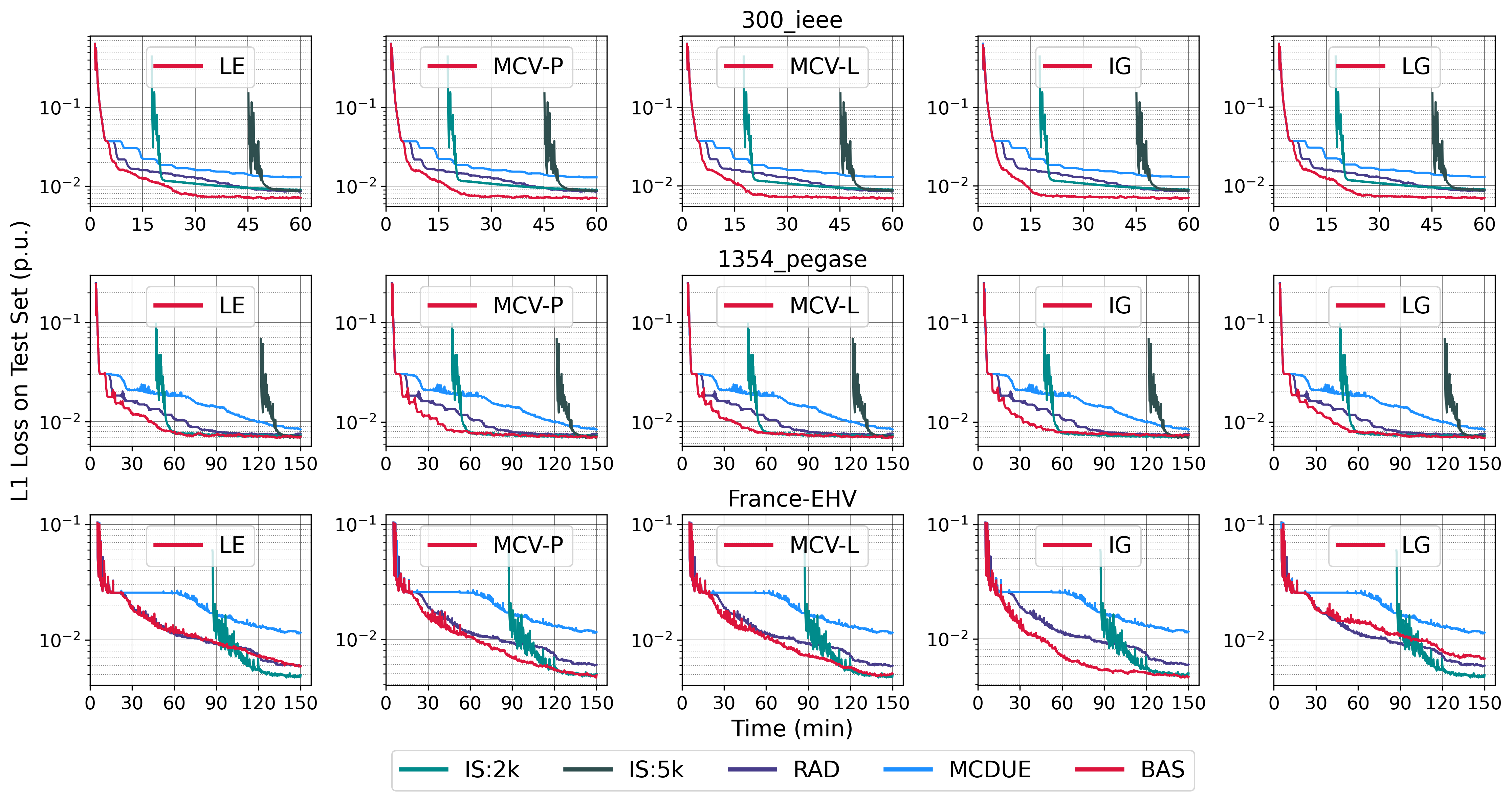
Figure 1: Mean L1 Loss on testing set, averaged across 50 trials.

IV-D Patience-based Scheduling

Another novelty of BAS is its use of patience-based scheduling, inspired by ReduceLROnPlateau [33]. BAS uses two patience counters $\rho_{1}$ and $\rho_{2}$. Counter $\rho_{1}$ is paired with $\gamma_{1}$, the classical discount factor ($\gamma_{1}<1.0$), to reduce the learning rate $\beta$ when $\rho_{1}$ reaches its threshold $\overline{\rho_{1}}$. When $\rho_{2}$ reaches its threshold, active sampling is triggered. In addition, to avoid premature learning convergence when new samples are added, BAS uses a boosting factor $\gamma_{2}>1.0$ to increase the learning rate. Algorithm 4 describes the procedure.

V Experimental Evaluation

Experiments are performed on 8 Intel Xeon 6226 CPU (2.7 GHz) machines, each with 192GB RAM. A Tesla V100-32GB GPU is used for training DNNs. Customized Julia 1.8.2 implementations using nonlinear solver Ipopt [34] with linear solver MA57 [35] are used to compute ACOPF solution data sets, and active learning experiments are implemented in Python 3.9.12 [36] with PyTorch 1.11.0 [33].

V-A Benchmarks

The experimental results are presented for public benchmark power networks 300_ieee and 1354_pegase from PGLib [37] as well as France-EHV, an industrial proprietary benchmark with 1737 buses, 1731 loads, 290 generators, and 2350 lines/transformers.

V-B Bucket-Validation Set Construction

The evaluation uses Algorithm 1 to generate datasets with $\mathfrak{B}=\text{Uniform}(0.8,1.2)$ and $\mathfrak{E}=\text{LogNormal}(0,0.05)$. For simplicity, $\mathfrak{D}_{B_{i}}$ is defined as a projection from the original sampling distribution $\mathfrak{D}_{U}$ onto the domain/feasible space of each bucket $B_{i}$. In other words, each bucket $B_{i}$ contains samples $\mathbf{x}_{j}$ whose load factor $b_{j}$ is within the lower/upper bounds $\underline{b_{i}}/\overline{b_{i}}$: $\left(\mathbf{x}_{j}\sim\mathfrak{D}_{B_{i}}\right)\equiv\left(\mathbf{x}_{j}\sim\mathfrak{D}\mbox{ where }b_{j}\in[\underline{b_{i}},\overline{b_{i}}]\right)$. All buckets of the bucket-validation set have $\lfloor\frac{n_{V}}{k}\rfloor$ feasible samples except for the last bucket which may have less. The evaluation uses $n_{V}=1024$ and $k=30$.

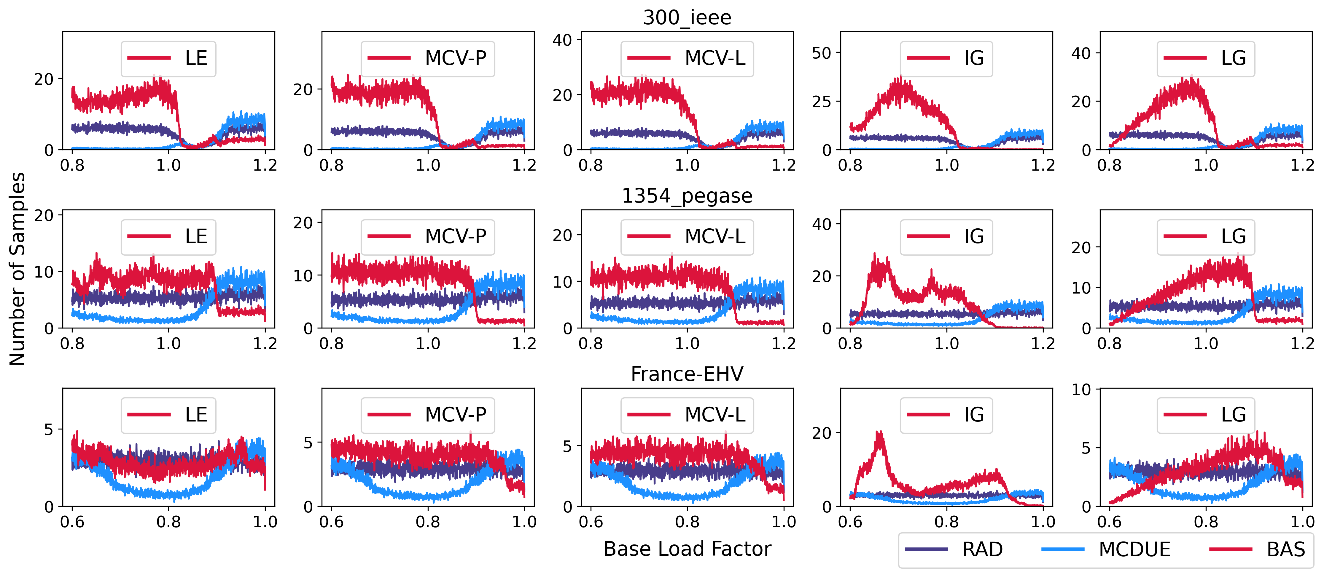
Figure 2: Mean sampling distributions across 50 trials.

V-C Learning Models

All experiments use fully connected DNNs with Sigmoid activation functions. Hidden layer dimensions are set to match the prediction feature size $2|\mathcal{G}|+|\mathcal{N}|+|\mathcal{E}|$. 1354_pegase and France-EHV experiments use 5 hidden layers while 300_ieee experiments use 3. The training uses a mini-batch size of 128, the AdamW optimizer [38], and the L₁ norm as the loss function. 256 samples are labeled to create an initial training set and 5000 testing samples are used for evaluations. Models are trained for at most 150 minutes, including training set solve time. Results are reported on held-out test data and are averaged over 50 trials using different random seeds.

BAS is compared with three baseline methods:

1. Inactive Sampling (IS): training data is pre-generated by sampling uniformly from the input domain.

2. Random Active Sampling (RAD): an active method that selects samples uniformly from the input domain.

3. Monte-Carlo Dropout Uncertainty Estimation (MCDUE): the state-of-the-art active method from [18].

Inactive sampling is used to show the benefits of sampling data actively. MCDUE is a state-of-the-art method in active learning, with the number of trails $\tau=25$ as in [18]. At every iteration, a pool of 5000 unlabeled samples is generated uniformly from the input domain for MCDUE to select from.

V-D Learning Quality: Accuracy & Convergence

Figure 1 presents the prediction accuracy (L1-loss) over the training period. Each row corresponds to a different grid, and each column corresponds to a different acquisition function. Overall, the prediction accuracy of BAS is consistently better than the other approaches. Both RAD and MCDUE take significantly more time to match the level of accuracy of BAS. Even though classic generate-then-train (IS) approaches may converge faster, they suffer from the significant amount of time needed to pre-generate data samples. Observe also that BAS-IG consistently has the lowest prediction errors over the training horizon. Interestingly, MCV-P, MCV-L, and IG converge faster than LE and LG.

V-E Sampling Behavior of Acquisition Functions

Figure 2 shows the distribution of samples, explaining why BAS-IG is most effective. Observe the fundamentally different sampling behavior of IG compared to the other acquisition functions. LE, MCV-P, and MCV-L have no clear preferences across buckets (except in the higher ranges of base loads, which will be discussed shortly), reducing the benefits of active learning. LG has a clear bias towards samples with higher base loads, as it uses the gradient of the loss with respect to the last layer. In contrast, IG has a much more differentiated sampling pattern. Because it uses the gradient of loss with respect to the input features, IG isolates highly sensitive regions of the input space. These samples trigger significant weight updates, even after passing through all the DNN layers during back-propagation. Thus, IG captures information from both forward evaluations and backward propagations. LE, MCV-P, and MCV-L mostly capture forward-information (prediction and loss), and fail to differentiate the different regions. LG has too large a bias towards samples with large outputs.

TABLE I: Mean number of samples generated across 50 trials

	300_ieee		1354_pegase		France-EHV
	Feasible	Infeasible	Feasible	Infeasible	Feasible	Infeasible
RAD	3275	2613	3937	1477	2651	266
MCDUE	290	3462	1455	2078	1554	334
LE	8019	1406	6306	887	2556	274
MCV-P	10070	1000	7519	533	3621	214
MCV-L	10818	883	7723	483	3794	203
IG	11396	766	8860	135	5802	104
LG	8967	1129	6709	758	2718	264

Second, observe that all acquisition functions under-sample regions with high load factor (e.g., $>$1.1 for 1354_pegase), contrary to MCDUE. These regions contain many infeasible samples which are not realistic as they correspond to loads that are over either global or regional production capabilities. Uncertainty-based active sampling methods (e.g., MCDUE) select samples with the highest predictive variance, which often correspond to infeasible samples. In contrast, the bucket-validation set allows BAS to allocate computational resources efficiently by surgically sampling in feasibility-dense regions, which are more useful for learning. Table I highlights these observations further and shows that BAS-IG is also able to label many more samples within the allocated time, limiting the number of time-consuming infeasible samples and focusing on regions of the input space that are more sensitive but whose samples are typically cheaper to label.

VI Conclusion & Future Work

This paper proposed BAS, a novel bucketized active learning framework. The framework partitions the input distribution into buckets and labels data samples based on the bucketized input space. A key innovation of BAS is the use of a bucket-validation set to decide where new samples are needed, decoupling the decision about where to sample from the actual sample generation. BAS also adopts a new learning rate adjustment scheme, and incorporates multiple acquisition functions inspired by the literature. Experimental evaluation against state-of-the-art approaches indicates the superior performance of BAS on large ACOPF benchmarks. Future work to improve BAS includes dynamic schemes for the selection of validation sets and bucket partitioning, and cost-aware acquisition functions.

References

- [1] X. Sun, P. B. Luh, M. A. Bragin, Y. Chen, F. Wang, and J. Wan, “A decomposition and coordination approach for large-scale security constrained unit commitment problems with combined cycle units,” in IEEE Power & Energy Society General Meeting, 2017, pp. 1–5.
- [2] S. Tam, “Real-time security-constrained economic dispatch and commitment in the pjm: Experiences and challenges,” in FERC Software Conference, 2011.
- [3] S. Verma, V. Mukherjee et al., “Transmission expansion planning: A review,” in 3rd International Conference on Energy Efficient Technologies for Sustainability (ICEETS 2016). IEEE, 2016, pp. 350–355.
- [4] F. Fioretto, T. W. Mak, and P. Van Hentenryck, “Predicting ac optimal power flows: Combining deep learning and lagrangian dual methods,” in 34th AAAI Conference on Artificial Intelligence (AAAI), 2020, pp. 630–637.
- [5] Z. Yan and Y. Xu, “Real-time optimal power flow: A lagrangian based deep reinforcement learning approach,” IEEE Transactions on Power Systems (TPWRS), vol. 35, no. 4, pp. 3270–3273, 2020.
- [6] X. Pan, M. Chen, T. Zhao, and S. H. Low, “Deepopf: A feasibility-optimized deep neural network approach for ac optimal power flow problems,” IEEE Systems Journal, vol. 17, no. 1, pp. 673–683, 2023.
- [7] Y. Tang, K. Dvijotham, and S. Low, “Real-time optimal power flow,” IEEE Transactions on Smart Grid, vol. 8, no. 6, pp. 2963–2973, 2017.
- [8] F. Diehl, “Warm-starting ac optimal power flow with graph neural networks,” in Advances in Neural Information Processing Systems 32 (NeurIPS), 2019, pp. 1–6.
- [9] D. Owerko, F. Gama, and A. Ribeiro, “Optimal power flow using graph neural networks,” in 2020 IEEE International Conference on Acoustics, Speech and Signal Processing (ICASSP). IEEE, 2020, pp. 5930–5934.
- [10] W. Dong, Z. Xie, G. Kestor, and D. Li, “Smart-pgsim: Using neural network to accelerate ac-opf power grid simulation,” in 2020 International Conference for High Performance Computing, Networking, Storage and Analysis (SC20). IEEE, 2020, pp. 1–15.
- [11] A. S. Zamzam and K. Baker, “Learning optimal solutions for extremely fast ac optimal power flow,” in 11th IEEE International Conference on Communications, Control, and Computing Technologies for Smart Grids (SmartGridComm 2020). IEEE, 2019, pp. 1–6.
- [12] R. Canyasse, G. Dalal, and S. Mannor, “Supervised learning for optimal power flow as a real-time proxy,” in 8th IEEE Conference on Power & Energy Society Innovative Smart Grid Technologies (ISGT). IEEE, 2017, pp. 1–5.
- [13] K. Baker, “A learning-boosted quasi-newton method for ac optimal power flow,” in Workshop on Machine Learning for Engineering Modeling, Simulation and Design, 2020.
- [14] N. Guha, Z. Wang, M. Wytock, and A. Majumdar, “Machine learning for ac optimal power flow,” in 36th International Conference on Machine Learning (ICML), 2019.
- [15] W. Chen, S. Park, M. Tanneau, and P. Van Hentenryck, “Learning optimization proxies for large-scale security-constrained economic dispatch,” Electric Power Systems Research, vol. 213, p. 108566, 2022.
- [16] A. Kirsch, J. Van Amersfoort, and Y. Gal, “Batchbald: Efficient and diverse batch acquisition for deep bayesian active learning,” Advances in Neural Information Processing Systems 32 (NeurIPS), vol. 32, 2019.
- [17] J. T. Ash, C. Zhang, A. Krishnamurthy, J. Langford, and A. Agarwal, “Deep Batch Active Learning by Diverse, Uncertain Gradient Lower Bounds,” in 7th International Conference on Learning Representations (ICLR), 2020.
- [18] E. Tsymbalov, M. Panov, and A. Shapeev, “Dropout-based active learning for regression,” in 7th International Conference on Analysis of Images, Social Networks and Texts (AIST 2018). Springer, 2018, pp. 247–258.
- [19] D. Angluin, “Queries and Concept Learning,” Machine Learning, vol. 2, no. 4, pp. 319–342, 1988.
- [20] D. D. Lewis and J. Catlett, “Heterogeneous uncertainty sampling for supervised learning,” in Machine Learning Proceedings 1994: Proceedings of the Eighth International Conference. Morgan Kaufmann, 1994, p. 148.
- [21] P. Kumar and A. Gupta, “Active learning query strategies for classification, regression, and clustering: A survey,” Journal of Computer Science and Technology, vol. 35, no. 4, pp. 913–945, 2020.
- [22] P. Ren, Y. Xiao, X. Chang, P.-Y. Huang, Z. Li, B. B. Gupta, X. Chen, and X. Wang, “A survey of deep active learning,” ACM Computing Surveys (CSUR), vol. 54, no. 9, pp. 1–40, 2021.
- [23] J. Choi, I. Elezi, H.-J. Lee, C. Farabet, and J. M. Alvarez, “Active learning for deep object detection via probabilistic modeling,” in 2019 IEEE/CVF International Conference on Computer Vision (ICCV), 2021, pp. 10 264–10 273.
- [24] D. Wu, “Pool-based sequential active learning for regression,” IEEE Transactions on Neural Networks and Learning Systems, vol. 30, no. 5, pp. 1348–1359, 2018.
- [25] W. Cai, Y. Zhang, and J. Zhou, “Maximizing expected model change for active learning in regression,” in 13th IEEE International Conference on Data Mining (ICDM). IEEE, 2013, pp. 51–60.
- [26] L. N. Smith, “Cyclical learning rates for training neural networks,” in 2017 IEEE Winter Conference on Applications of Computer Vision (WACV). IEEE, 2017, pp. 464–472.
- [27] L. N. Smith and N. Topin, “Super-convergence: Very fast training of neural networks using large learning rates,” in Artificial Intelligence and Machine Learning for Multi-Domain Operations Applications, vol. 11006. International Society for Optics and Photonics, 2019, p. 12.
- [28] I. Loshchilov and F. Hutter, “Sgdr: Stochastic gradient descent with warm restarts,” Learning, vol. 10, p. 3, 2016.
- [29] M. Zaheer, S. Reddi, D. Sachan, S. Kale, and S. Kumar, “Adaptive methods for nonconvex optimization,” Advances in Neural Information Processing Systems 31 (NeurIPS 2018), vol. 31, 2018.
- [30] Z. Liu, H. Ding, H. Zhong, W. Li, J. Dai, and C. He, “Influence selection for active learning,” in 2021 IEEE/CVF International Conference on Computer Vision (ICCV), 2021, pp. 9274–9283.
- [31] S. Roy, A. Unmesh, and V. P. Namboodiri, “Deep active learning for object detection,” in 29th British Machine Vision Conference (BMVC 2018), 2018, p. 91.
- [32] Y. LeCun, Y. Bengio, and G. Hinton, “Deep learning,” Nature, vol. 521, no. 7553, pp. 436–444, 2015.
- [33] A. Paszke et al., “PyTorch: An Imperative Style, High-Performance Deep Learning Library,” in Advances in Neural Information Processing Systems 32, H. Wallach, H. Larochelle, A. Beygelzimer, F. d’Alché Buc, E. Fox, and R. Garnett, Eds. Curran Associates, Inc., 2019, pp. 8024–8035.
- [34] L. T. Biegler and V. M. Zavala, “Large-scale nonlinear programming using ipopt: An integrating framework for enterprise-wide dynamic optimization,” Computers & Chemical Engineering, vol. 33, no. 3, pp. 575–582, 2009.
- [35] I. S. Duff, “Ma57—a code for the solution of sparse symmetric definite and indefinite systems,” ACM Transactions on Mathematical Software (TOMS), vol. 30, no. 2, pp. 118–144, 2004.
- [36] G. Van Rossum and F. L. Drake, Python 3 Reference Manual. Scotts Valley, CA: CreateSpace, 2009.
- [37] S. Babaeinejadsarookolaee et al., “The Power Grid Library for Benchmarking AC Optimal Power Flow Algorithms,” IEEE PES PGLib-OPF Task Force, Tech. Rep., 2019.
- [38] I. Loshchilov and F. Hutter, “Decoupled weight decay regularization,” in 6th International Conference on Learning Representations (ICLR), 2018.