All-optical control of thermal conduction in waveguide QED

Abstract

We investigate the heat conduction between two one-dimension waveguides intermediated by a Laser-driving atom. The Laser provides the optical control on the heat conduction. The tunable asymmetric conduction of the heat against the temperature gradient is realized. Assisted by the modulated Laser, the heat conduction from either waveguide to the other waveguide can be suppressed. Meanwhile, the conduction towards the direction opposite to the suppressed one is gained. The heat currents can be significantly amplified by the energy flow of the Laser. Moveover, the scheme can act like a heat engine.

I Introduction

The scheme composed by one-dimension (1D) waveguides coupled to emitters, known as waveguide QED (Quantum Electrodynamics), has been studied extensively Colloquium ; fan07 ; shi ; fanthero ; zhengqed ; longo ; faninout ; roy ; zhou1 ; pla1 ; pla2 ; pla3 ; crys ; Nanofibe ; dark ; ChargeNoise ; Chaos ; Ratchet ; TopologyNonreciprocal ; giantLambda ; dipoleapproximation ; ultrastrong ; BoundPhotonicPairs ; twogiant ; Cavitylike ; Boundstates ; multiplecoupling ; gaintn ; Schrodinger ; Selforder ; Nonperturbative ; Bellstates ; nonMarkoviandynamics ; Modeling ; Multiphoton ; Amplification ; Transparency ; Implications ; MultipleFano ; Entanglementpreserving ; Phasemodulated ; interference ; Transmission ; Photonscattering . The 1D continuum guided photonic modes can be realized in several nanoscale schemes, such as surface plasmon of metallic nanowires pla1 ; pla2 ; pla3 , photonic crystal waveguides crys , optical nanofibers Nanofibe , and so on. Waveguide QED provides a potential platform for the management of few photons through light-emitter interaction.

On the other hand, the management and reuse of the wasted heat is a significant issue because the energy resources are limited and the energy utilization in industry is always accompanied by the heat lost. Recently, due to the development in engineering individual small scale devices, the management of the thermal conduction in the small scale devices has attracted extensive attention retc ; optimal ; Quantumthermaltransistor ; energybackflow ; threereservoirs ; interactingspinlike ; DynamicalCoulombblockade ; Allthermaltransistor ; ThermalNoise ; qubitqutritcoupling ; nonequilibriumtwoqubit ; Dynamicallyinduced ; nonequilibriumVtype ; twoatom ; wu ; collisionmodels ; utilizingthreequbits ; MobilityEdges ; Isingmodel ; segmentedXXZchains ; Searching ; criticalheat ; heattransport ; effectof ; heatflowres ; transistorinsuperconducting ; quantifyingheat ; Opticallycontrolledquantum ; bathspectralfiltering ; nonthermalbath ; incoupledcavities ; Quantumthermaltransistors ; ThermalTransistorEffec ; Redfield approach ; rectificationthroughnonlinear ; Darlingtonair ; DzyaloshinskiiMoriya ; Ballisticthermal ; Decoupledheatcharge ; Steadyentanglement ; Coherencehanced ; diodeandcirculator ; Entanglementenhanced ; multitransistor ; Geometrybasedcirculation ; CycleFluxRanking ; coupledquantumdots ; threesuperconductingcircuit ; Correlationenabled . A large number of the works focus on the realization of the thermal quantum devices analogous to the electronic components, such as the diode-like retc ; optimal and transistor-like Quantumthermaltransistor operations. In the thermal diode-like operations, the heat conduction towards the fixed direction is significantly suppressed while the opposite direction is allowed. It will be of interest to realize the tunable thermal diode-like operation, in which the suppressed conduction direction can be artificially selected by tunable parameters. More interestingly, due to the experimental operability, waveguide QED may provide a potential platform for the thermal devices, which needs to be explored.

Though the individual quantum thermal device has been studied extensively with great progress, it deserves a deep study how to integrate them for the applicable purpose. Waveguide QED may provide a potential platform for this based on two facts. One is that waveguide QED provides a potential candidate for the quantum network qn by integrating the waveguides and emitters into a large system BoundPhotonicPairs , in which the waveguides act as the channels and the emitters as the nods. The other is that the locations and numbers of the emitters coupled to the waveguide can be accurately manipulated in most of the practical implementations. The latter implies that waveguide QED would show significant advantages of individually managing the thermal conduction of each quantum thermal device in the integrated system. It is necessary to note that the individual management is essential but challenging. A potential approach to overcome this is to develop the control on the thermal conduction by optical modulation Opticallycontrolledquantum , compared to the thermal modulation Quantumthermaltransistor . Therefore, provided that the heat conduction in waveguides can be managed by the optical signal acting on the emitter, it is reasonable to believe that waveguide QED will provide significant help to the integrated thermal quantum devices.

For these purposes, we propose to control the heat conduction by the optical signals based on waveguide QED. In our scheme, the heat conduction between two 1D waveguides is assisted by an intermediate emitter, which is coupled to the continuum photonic modes of the two waveguides. We employ two weak Laser beams to drive the intermediate emitter and show that the heat conduction can be controlled by the Laser beams. The heat conduction shows asymmetry against the temperature gradient for appropriate laser parameters. In the ideal case, assisted by the optically modulated Laser, either direction of the heat conduction between the two waveguides can be prohibited while the opposite direction is gained. In the nonideal case, either direction can be significantly suppressed while the opposite direction is gained. This provides the rectification and switch of the heat conduction by the optical modulation. The heat currents of the waveguides largely change when the energy flow of the Laser changes slightly. Therefore, the scheme shows the thermal transistor-like operation. Besides, the scheme can convert the heat to work, which can be considered as the engine-like operation. Our investigation provides a potential advantageous quantum-optic platform to the thermal management.

This paper is organized as follows. In Sec. II, we introduce the scheme and Hamiltonian of the system. In Sec. III, we obtain the time evolution of reduced density operator for the emitter in the weak coupling regime and discuss the elements of the density matrix. In Sec. IV, we investigate the energy properties in the steady-state regime. The control of heat conduction by optical modulation and the engine-like operation are demonstrated. In Sec. V, the conclusion and necessary discussions are made.

II Model and Hamiltonian

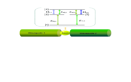
Figure 1: An four-level atom driven by two Laser beams is side-coupled to two 1D waveguides.

The schematic diagram of the considered system is shown in Fig. 1. A four-level emitter is side-coupled to two 1D waveguides. The emitter could be a real atom or a manual atom-like object, such as the quantum dot crys coupled to the plasmonic or photonic-crystal waveguide. The four atomic states are denoted by $\left|j\right\rangle$ ($j=1,2,3,4$), with the corresponding level frequencies $\omega_{j}$. The atomic transitions $\left|2\right\rangle\leftrightarrow\left|1\right\rangle$ and $\left|4\right\rangle\leftrightarrow\left|3\right\rangle$ are coupled to the guided photons in the waveguide 1 with strengths $g_{21,k}$ and $g_{43,k}$, respectively. The atomic transitions $\left|3\right\rangle\leftrightarrow\left|1\right\rangle$ and $\left|4\right\rangle\leftrightarrow\left|2\right\rangle$ are coupled to the guided photons in the waveguide 2 with strengths $g_{31,k}$ and $g_{42,k}$, respectively. The symbol $k$ denotes the wave vector of the guided photon. Here, we assume that the values of elements in the set $\{\omega_{43},\omega_{42}\}$ are obviously different from the ones in $\{\omega_{21},\omega_{31}\}$, with $\omega_{jj^{\prime}}=\omega_{j}-\omega_{j^{\prime}}$ the atomic transition frequency. The external laser beam with frequency $\omega_{L_{43}}$ ($\omega_{L_{42}}$) and Rabi frequency $\Omega_{43}$ ($\Omega_{42}$) is introduced to drive the atomic transition $\left|4\right\rangle\leftrightarrow\left|3\right\rangle$ ($\left|4\right\rangle\leftrightarrow\left|2\right\rangle$) through polarization and frequency selections. We assume that the atom-waveguide and atom-Laser coupling strengths are much smaller than the corresponding atomic transition frequencies. Hereafter, we take reduced Plank constant $\hbar=1$. Within the rotating-wave approximation, the Hamiltonian governing the system is

$$H=H_{A}+H_{W}+H_{A-W}+H_{A-L}$$

with

$$H_{A} = \sum_{j=1...4}\omega_{j}\sigma^{jj},$$

$$H_{W} = \sum_{k}\omega_{1,k}b_{1,k}^{\dagger}b_{1,k}+\sum_{k}\omega_{2,k}b_{2,k}^{\dagger}b_{2,k},$$

$$H_{A-W} = \sum_{k}(g_{21,k}\sigma^{21}b_{1,k}+g_{31,k}\sigma^{31}b_{2,k}$$

$$+g_{43,k}\sigma^{43}b_{1,k}+g_{42,k}\sigma^{42}b_{2,k})+h.c.$$

$$H_{A-L} = \Omega_{42}\sigma^{42}e^{-i\omega_{L42}t}+\Omega_{43}\sigma^{43}e^{-i\omega_{L43}t}+h.c.$$ (1)

with the operator $\sigma^{jj^{\prime}}=\left|j\right\rangle\left\langle j^{\prime}\right|$ denoting the atomic raising, lowering, and energy-level population operators, and the operator $b_{m,k}^{\dagger}$ ($b_{m,k}$) creating (annihilating) a photon with wave vector $k$ in the waveguide $m$. The symbol $\omega_{m,k}$ ($m=1,2$) denotes the photonic frequency in waveguide $m$. We consider that the guided photonic frequency is far from the waveguide cutoff frequency and hence the guided photonic dispersion relation is approximately linearized. The Hamiltonian $H_{A}$ denotes the atomic energy, $H_{W}$ represents the energy of the guided photon in the two waveguides, $H_{A-W}$ describes the coupling of the atom to the two waveguides, and $H_{A-L}$ denotes the interaction between the atom and the external Laser beams.

III Quantum Master Equation

The time evolution of the reduced density operator for the atom $\rho_{A}$ is obtained based on the approach represented in qo . We assume that the guided modes are distributed in the uncorrelated thermal equilibrium mixture of states and hence the two waveguides are considered as two thermal reservoirs. Consequently, one can obtain $\left\langle b_{m,k}\right\rangle=\left\langle b_{m,k}^{\dagger}\right\rangle=0$, $\left\langle b_{m,k}b_{m^{\prime},k^{\prime}}\right\rangle=\left\langle b_{m,k}^{\dagger}b_{m^{\prime},k^{\prime}}^{\dagger}\right\rangle=0$, $\left\langle b_{m,k}b_{m^{\prime},k^{\prime}}^{\dagger}\right\rangle=(n_{\omega_{k},m}+1)\delta_{m,m^{\prime}}\delta_{k,k^{\prime}}$, and $\left\langle b_{m,k}^{\dagger}b_{m^{\prime},k^{\prime}}\right\rangle=n_{\omega_{k},m}\delta_{m,m^{\prime}}\delta_{k,k^{\prime}}$, with

$$n_{\omega_{k},m}=[\exp(\frac{\omega_{m,k}}{k_{B}T_{m}})-1]^{-1}$$

the average occupation number of the photons with wave vector $k$ in the reservoir $m$. The symbol $T_{m}$ represents temperature of the reservoir $m$ and $k_{B}$ denotes Boltzmann constant. The Hamiltonian (1) can be mapped to the interaction picture as $H^{I}(t)=e^{iH_{0}t}H_{I}e^{-iH_{0}t}$, with $H_{0}=H_{A}+H_{W}$, and $H_{I}=H_{A-W}+H_{A-L}$. From the interaction picture von Neumann equation, one can obtain

$$\dot{\rho}_{A}^{I}(t) = -iTr_{W}[H^{I}(t),\rho_{total}^{I}(t_{0})]$$ (2)

$$-Tr_{W}\int_{t_{0}}^{t}dt^{\prime}[H^{I}(t),[H^{I}(t^{\prime}),\rho_{total}^{I}(t^{\prime})]],$$

where $\rho_{A}^{I}(t)$ represents the interaction-picture reduced density operator for the atom, $\rho_{total}^{I}(t)$ is the interaction-picture density operator of the atom-waveguide system, and $Tr_{W}$ denotes the partial trace through the waveguides. Inserting $H^{I}(t)$ into Eqn. (2) and performing Born, secular, and Weisskopf-Wigner approximations, we can derive the master equation representing the time evolution of $\rho_{A}^{I}(t)$ in the weak coupling regime (see Appendix for details). Turning back to Schrödinger picture, the evolution of the reduced matrix for the atom is given as

$$\dot{\rho}_{A}=-i[H_{A}+H_{A-L},\rho_{A}]+\sum_{lp}\mathcal{L}_{lp}[\rho_{A}],$$ (3)

with $lp\in\{21,31,42,43\}$. The dissipative Lindblad superoperator $\mathcal{L}_{lh}[\rho_{A}]$ has the form of

$$\mathcal{L}_{lp}[\rho_{A}] = \gamma_{lp}(n_{\omega_{lp}}+1)(\sigma^{pl}\rho_{A}\sigma^{lp}-\frac{1}{2}\{\sigma^{ll},\rho_{A}\})$$

$$+\gamma_{lp}n_{\omega_{lp}}(\sigma^{lp}\rho_{A}\sigma^{pl}-\frac{1}{2}\{\sigma^{pp},\rho_{A}\}),$$

where $\gamma_{lp}$ denotes the atomic decay to the waveguide accompanied by the transition $\left|l\right\rangle\leftrightarrow\left|p\right\rangle$ (see Appendix for details). Here, we have labeled $n_{\omega_{jj^{\prime}},m}\rightarrow n_{\omega_{jj^{\prime}}}$ because each atomic transition is coupled to its designated reservoir.

We focus on the steady-state regime. The master equation of Eqn. (3) contains the time-dependent phase. It will be convenient to look for a rotating frame in which the steady-state reduced density operator is time-independent. We bring in the rotating frame with respect to $H^{\prime}=-\omega_{L42}\sigma^{22}-\omega_{L43}\sigma^{33}$. The arbitrary operator $O$ has the form of $O^{\prime}=e^{iH^{\prime}t}Oe^{-iH^{\prime}t}$ in the rotating frame. In this frame, the atomic Hamiltonian $H_{A}$ keeps unchanged and the time evolution of the reduced density operator for the atom turns out to be

$$\dot{\rho}=-i[H_{A}-H^{\prime}+H_{A-L}^{\prime},\rho]+\sum_{lp}\mathcal{L}_{lp}[\rho],$$ (4)

with $H_{A-L}^{\prime}=\Omega_{42}\sigma^{42}+\Omega_{43}\sigma^{43}+h.c.$ The Hamiltonian in the first term of the right hand in Eqn. (4) is time-independent. The time evolution of the density matrix diagonal elements are obtained as

$$\dot{\rho}_{11} = \Gamma_{21}+\Gamma_{31},$$

$$\dot{\rho}_{22} = \Gamma_{42}-\Gamma_{21}-\Upsilon_{42},$$

$$\dot{\rho}_{33} = \Gamma_{43}-\Gamma_{31}-\Upsilon_{43},$$

$$\dot{\rho}_{44} = -\Gamma_{43}-\Gamma_{42}+\Upsilon_{42}+\Upsilon_{43},$$ (5)

where $\rho_{jj^{\prime}}=\left\langle j\right|\rho\left|j^{\prime}\right\rangle$, $\Gamma_{jj^{\prime}}={\gamma_{jj^{\prime}}[}\left({n_{\omega_{jj^{\prime}}}}+1\right)\rho_{jj}-{n_{\omega_{jj^{\prime}}}}\rho_{j^{\prime}j^{\prime}}]$ denotes the net decay rate from $\left|j\right\rangle$ to $\left|j^{\prime}\right\rangle$ due to the atom-reservoir interaction, and $\Upsilon_{jj^{\prime}}=i\Omega_{jj^{\prime}}\left(\rho_{jj^{\prime}}-\rho_{j^{\prime}j}\right)$ is the net transition resulting from the atom-Laser interaction. The off-diagonal elements $\rho_{42}$ and $\rho_{43}$ have the direct impact on the time evolution of the diagonal elements, and $\rho_{32}$ has the indirect impact on the diagonal elements. Their evolutions are obtained as

$$\dot{\rho}_{42} = -i(\omega_{42}-\omega_{L42})\rho_{42}+\alpha_{42}-\eta_{432}$$

$$-\frac{\beta_{42}^{+}+\beta_{42}^{-}+\beta_{43}^{+}+\beta_{21}^{+}}{2}\rho_{42},$$

$$\dot{\rho}_{43} = -i(\omega_{43}-\omega_{L43})\rho_{43}+\alpha_{43}-\eta_{423}$$

$$-\frac{\beta_{43}^{+}+\beta_{43}^{-}+\beta_{42}^{+}+\beta_{31}^{+}}{2}\rho_{43},$$

$$\dot{\rho_{32}} = -i[\omega_{32}-(\omega_{{L42}}-\omega_{{L43}})]\rho_{32}-\eta_{243}^{\ast}+\eta_{342}^{\ast}$$ (6)

$$-\frac{\beta_{31}^{+}+\beta_{21}^{+}+\beta_{43}^{-}+\beta_{42}^{-}}{2}\rho_{32},$$

with $\alpha_{jj^{\prime}}=i\Omega_{jj^{\prime}}\left(\rho_{jj}-\rho_{j^{\prime}j^{\prime}}\right)$, $\beta_{jj^{\prime}}^{+}=({n_{\omega_{jj^{\prime}}}}+1){\gamma_{jj^{\prime}}}$, $\beta_{jj^{\prime}}^{-}={n_{\omega_{jj^{\prime}}}\gamma_{jj^{\prime}}}$, $\eta_{jj^{\prime}j^{\prime\prime}}=i\Omega_{jj^{\prime}}\rho_{j^{\prime}j^{\prime\prime}}$. For simplicity, the Rabi frequency $\Omega_{42}$ ($\Omega_{43}$) has been labeled as $\Omega_{24}$ ($\Omega_{34}$) somewhere. The first term of the right hand of the first equation in Eqns. (6) disappears when the atomic transition $\left|4\right\rangle\leftrightarrow\left|2\right\rangle$ is resonantly driven by the Laser. The second and third terms result from the atom-Laser interactions, and the forth term is caused by the atom-reservoir coupling. The other two equations can be interpreted in a similar way. Other density matrix elements other than the ones given in Eqns. (5-6) have no impact on the ones given in Eqns. (5-6) due to the expression of each term in our master equation.

IV Heat Currents Controlled by Optical Modulation

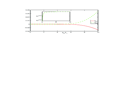
Figure 2: Heat currents against the temperature of the reservoir 1 when the Laser driving the atomic transition $|4\rangle\leftrightarrow|3\rangle$ is shut off and $T_{2}\rightarrow 0$. The red solid line represents the current into the reservoir 1 and the green dashed line denotes the current into the reservoir 2. The parameters are $\omega_{1}$=0, $\omega_{2}=\omega_{3}=50\gamma_{21}$, $\omega_{4}=70\gamma_{21}$, $\Omega_{42}=\gamma_{21}$, $\gamma_{31}=\gamma_{21}$, $\omega_{L42}=\omega_{42}$, and $\gamma_{42}=\gamma_{43}=0.2\gamma_{21}$.

The average energy of the atom is $\left\langle H_{A}\right\rangle=Tr(H_{A}\rho)$. The time evolution of the average energy going through the atom is given as

$$\frac{\partial\left\langle H_{A}\right\rangle}{\partial t}=Tr(H_{A}\dot{\rho})=J_{L}^{in}+\sum_{m=1,2}J_{Wm}^{in},$$ (7)

with $J_{L}^{in}=-iTr(H_{A}[H_{A-L}^{\prime},\rho])$, or alternatively $J_{L}^{in}=-iTr([H_{A},H_{A-L}^{\prime}]\rho)$, describing the energy flow from the Laser. Moreover, the energy flow can be divided into two parts as

$$J_{L1}^{in} = -iTr(H_{A}[\Omega_{42}\sigma^{42}+h.c.,\rho]),$$

$$J_{L2}^{in} = -iTr(H_{A}[\Omega_{43}\sigma^{43}+h.c.,\rho]).$$ (8)

The two parts respectively denote the energy flow from either Laser beam. The heat currents from the reservoirs are

$$J_{W1}^{in} = Tr(H_{A}\mathcal{L}_{21}[\rho])+Tr(H_{A}\mathcal{L}_{43}[\rho]),$$

$$J_{W2}^{in} = Tr(H_{A}\mathcal{L}_{31}[\rho])+Tr(H_{A}\mathcal{L}_{42}[\rho]).$$

Then the heat current injected into either reservoir is

$$J_{Wm}=-J_{Wm}^{in}.$$

Obviously, $J_{Wm}>0$ implies that the heat is injected into reservoir $m$, and $J_{Wm}<0$ implies the outflow of heat from the reservoir $m$. Similarly, the energy flow into the Laser beam is

$$J_{Lm}=-J_{Lm}^{in}.$$

In the steady-state regime, i.e. $\dot{\rho}=0$, the average energy of the atom does not change against time, and hence $\sum_{m=1,2}(J_{Lm}+J_{Wm})=0$. It implies that the steady state of the waveguide-emitter system can be the nonequilibrium state. In the nonequilibrium state, there are energy exchanges among the four light fields, i.e. the two guided continuum modes and the two Laser beams. The conservation of energy is fulfilled.

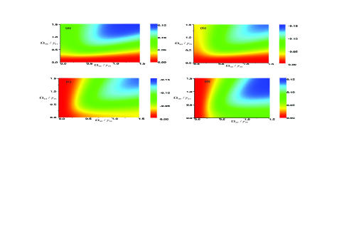
Figure 3: Heat currents against the Rabi frequencies of the Laser beams. (a) and (b) represent the case when $k_{B}T_{1}=1$ and $k_{B}T_{2}=10$. (c) and (d) represent $k_{B}T_{1}=10$ and $k_{B}T_{2}=1$. (a) and (c) denote the current $J_{W1}$ against the Rabi frequencies. (b) and (d) denote $J_{W2}$. The parameters are $\omega_{1}=0$, $\omega_{2}=\omega_{3}=50\gamma_{21}$, $\omega_{4}=70\gamma_{21}$, $\omega_{L42}=\omega_{42}$, $\omega_{L43}=\omega_{43}$, $\gamma_{31}=\gamma_{21}$, and $\gamma_{42}=\gamma_{43}=0.2\gamma_{21}$.

From the expressions of $J_{Lm}$ and $J_{Wm}$, the density matrix elements given in Eqns. (5-6) are enough to investigate $J_{Lm}$ and $J_{Wm}$. To obtain the steady-state solution, it is necessary to consider the condition $\sum_{j}\rho_{jj}=1$. This is because the sum of the four equations in Eqns. (5) is zero, i.e. $Tr\dot{\rho}=0$.

IV.1 Control of heat conduction by optical modulation

In our scheme, it is possible to realize the diode-like behavior for the heat currents, i.e. the asymmetric conduction of the heat against the temperature gradient, if either of the two Laser beams is shut off. To show this, we first consider the situation when $\Omega_{43}=0$ and $\Omega_{42}\neq 0$. In the ideal cases when $T_{1}\rightarrow 0$ and $T_{2}>0$, by solving Eqns. (5-6), the steady-state density matrix elements are obtained as

$$\rho_{11} \rightarrow \frac{n_{31}+1}{2n_{31}+1},$$

$$\rho_{33} \rightarrow \frac{n_{31}}{2n_{31}+1},$$ (9)

and other elements tend to zero. Then, the heat currents into the reservoirs are obtained as $J_{L1}\rightarrow 0$ and $J_{L2}\rightarrow 0$. Therefore, the heat conduction from the reservoir 2 to the reservoir 1 is prohibited although $T_{2}\gg T_{1}$. Conversely, the heat conduction from the reservoir 1 to the reservoir 2 is allowed if $T_{2}\rightarrow 0$ and $T_{1}>0$, which is verified by the numerical simulation as shown in Fig. 2.

The diode-like operation realized when $\Omega_{43}=0$ and $\Omega_{42}\neq 0$ can be understood by the fact that the heat conduction from one reservoir to the other is assisted by the cycle of atomic transitions, such as $\left|1\right\rangle\rightarrow\left|3\right\rangle\rightarrow\left|4\right\rangle\rightarrow\left|2\right\rangle\rightarrow\left|1\right\rangle$, $\left|1\right\rangle\rightarrow\left|2\right\rangle\rightarrow\left|4\right\rangle\rightarrow\left|3\right\rangle\rightarrow\left|1\right\rangle$, or other cycles. The atomic transition from level $\left|3\right\rangle$ to $\left|4\right\rangle$ needs absorbing the energy from the laser beam or the reservoir 1, and the transition $\left|1\right\rangle$ to $\left|2\right\rangle$ needs absorbing the energy from the reservoir 1. Obviously, when $T_{1}\rightarrow 0$ and $\Omega_{43}=0$, both the two atomic transitions will not be realized. Hence, all the atomic transition cycles that are helpful to the heat conduction between the two reservoirs can not be achieved. As a result, the heat conduction is forbidden although $T_{2}\gg T_{1}$. In this case, the system, which can be considered as a two-level atom (TLA) with levels $\left|3\right\rangle$ and $\left|1\right\rangle$ coupled to the reservoir 2, is in the thermal equilibrium state. The steady-state solution in Eqns. (9) implies that the TLA is in the Gibbs thermal state $\frac{e^{-\beta H_{TLA}}}{Tr(e^{-\beta H_{TLA}})}$ with $H_{TLA}=\omega_{1}\sigma^{11}+\omega_{3}\sigma^{33}$ representing the energy of the TLA. The effective temperature of the TLA, i.e. $T_{eff}=\frac{\omega_{31}}{k_{B}}[\ln\frac{\rho_{11}}{\rho_{33}}]^{-1}$, tends to $T_{2}$. As $T_{2}$ increases, $\rho_{33}$ increases. When $T_{2}\rightarrow\infty$, both $\rho_{11}$ and $\rho_{33}$ tend to $1/2$. For the reversed temperature gradient, i.e. $T_{2}\rightarrow 0$ and $T_{1}>0$, the helpful atomic transition cycles are feasible and hence the heat conduction is realized. It is interesting to note that the heat conduction absorbed by the cold reservoir is larger than the conduction left from the hot reservoir in Fig. 2, which implies the gain of the heat current. This is because the energy of the Laser beam is converted into the heat during the atomic transition cycle.

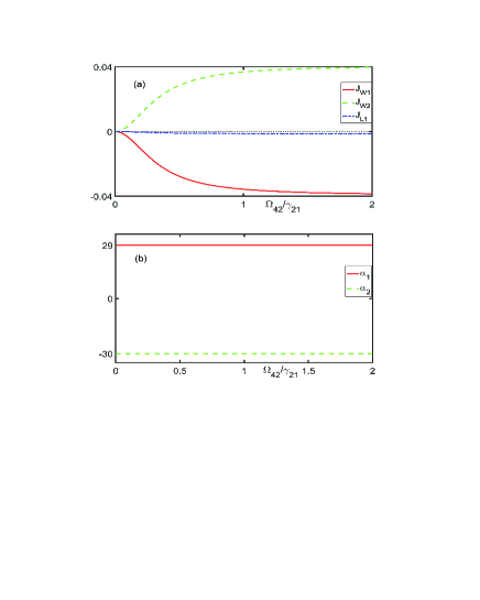
Figure 4: Numerical simulation the amplification of the heat currents of the reservoirs by the Laser. (a) shows $J_{W1}$, $J_{W2}$, and $J_{L1}$ against the Rabi frequency $\Omega_{42}$, represented by the red solid, green dashed, and blue dashed dotted lines, respectively. (b) shows the amplification factors $\alpha_{1}$ and $\alpha_{2}$, represented by the red solid and green dashed lines, respectively. The parameters are $k_{B}T_{1}=10$, $k_{B}T_{2}=1$, $\omega_{1}=0$, $\omega_{2}=\omega_{3}=60\gamma_{21}$, $\omega_{4}=62\gamma_{21}$, $\Omega_{43}=\gamma_{42}=0$, $\omega_{L42}=\omega_{42}$, $\gamma_{31}=\gamma_{21}$, and $\gamma_{43}=0.1\gamma_{21}$.

Similarly, if the Laser beam driving the atomic transition $\left|4\right\rangle\leftrightarrow\left|3\right\rangle$ is turned on while the beam driving $\left|4\right\rangle\leftrightarrow\left|2\right\rangle$ is shut off, the heat conduction is forbidden (gained) when $T_{2}\rightarrow 0$ and $T_{1}>0$ ($T_{1}\rightarrow 0$ and $T_{2}>0$). Shutting off the different Laser beams forbids the heat currents towards the different directions, respectively. Therefore, in the ideal case when the temperature of the cold reservoir approaches zero, the heat conduction towards either direction can be optimally suppressed while the conduction along the opposite direction is gained.

Besides the ideal case, when the temperature of the cold reservoir is nonzero, the pronounced asymmetric conduction of the heat against the temperature gradient can also be realized. In Fig. 3, we plot the heat currents against the Rabi frequencies of the Laser beams. We consider that the two reservoirs are symmetrical to the four-level atom, i.e. $\omega_{2}=\omega_{3}$, $\gamma_{21}=\gamma_{31}$, and $\gamma_{43}=\gamma_{42}$. The plots show the pronounced asymmetric conduction of the heat when the atom-Laser couplings are pronounced asymmetric, i.e. $\max\{\Omega_{43},\Omega_{42}\}/\min\{\Omega_{43},\Omega_{42}\}\gg 1$. The fact that either of the two Laser beams is shut off is the special case of the asymmetric atom-Laser coupling. The heat conduction from reservoir 1 to 2 is significantly suppressed when $\Omega_{42}\$is small enough. Conversely, the conduction from reservoir 2 to 1 is significantly suppressed when $\Omega_{43}\$ is small enough. The minimum currents for the asymmetric conduction into the cold reservoir, i.e. in Fig. 3 (a) and (d), are in the order of $10^{-11}$. The heat transporting towards the allowed directions is gained by the Laser beams, which can be interpreted by comparing the currents of the cold and hot reservoirs. Therefore, the scheme provides the control of the heat conduction by the optical modulation of the Laser.

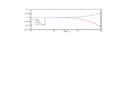
Figure 5: The energy flows against the temperature of the reservoir 1 when $k_{B}T_{2}=1$. The red solid line represents the heat current into the reservoir 1, the green dashed line denotes the heat current into the reservoir 2, and the blue dashed dotted line shows the energy flow into the Lasers. The parameters are $\omega_{1}$=0, $\omega_{2}=50\gamma_{21}$, $\omega_{3}=25\gamma_{21}$, $\omega_{4}=60\gamma_{21}$, $\omega_{L43}=\omega_{43}$, $\omega_{L42}=\omega_{42}$, $\Omega_{42}=\Omega_{43}=\gamma_{21}$, $\gamma_{31}=\gamma_{21}$, and $\gamma_{42}=\gamma_{43}=0.1\gamma_{21}$.

In an electronic transistor, the currents of the collector and emitter can be modulated, switched and amplified by the base current. The modulation and switch of the heat currents by the base current have been realized if we consider the energy flow of the Laser as the base current. We proceed to show that the heat currents of the two reservoirs can be amplified by the Laser, i.e. the heat currents change significantly when the energy flow of the Laser varies slightly. Followed by the definition in Ref. Quantumthermaltransistor , the dynamical amplification factor for either heat current is $\alpha_{m}=\frac{\partial J_{Wm}}{\partial J_{L}}$. The numerical simulations in Fig. 4 show that the significant amplification of the heat currents by the Laser can be realized. To clearly understand the amplification we assume that the Laser beam driving the transition $\left|4\right\rangle\leftrightarrow\left|3\right\rangle$ is shut off and the transition $\left|4\right\rangle\leftrightarrow\left|2\right\rangle$ is decoupled to the reservoir 2 in Fig. 4. The decoupling of the waveguide to a certain atomic transition is feasible for appropriate cutoff frequency of the waveguide so that the photon with frequency around the corresponding atomic transition frequency can not transport in the waveguide. In this case, the heat conduction from reservoir $1$ to $2$ is assisted by the atomic clockwise transition cycle. The amplification results from the fact that the frequency of the Laser resonantly driving $\left|4\right\rangle\leftrightarrow\left|2\right\rangle$ is significantly smaller than the frequencies of the guided photons driving the atom, i.e. the behaviors of the amplification factors in Fig. 4 are $\left|\alpha_{1}\right|\rightarrow\frac{\omega_{21}-\omega_{43}}{\omega_{42}}$ and $\left|\alpha_{2}\right|\rightarrow\frac{\omega_{31}}{\omega_{42}}$.

IV.2 Engine-like operation

The goal of a heat engine is to convert the heat energy from the reservoirs to work. Therefore, the steady-state current $\sum_{m}J_{Wm}<0$, or alternatively $\sum_{m}J_{Lm}>0$, implies an engine-like operation. For example, considering the case when the clockwise atomic transition cycle is dominant in dynamic evolution, it would be feasible to realize a positive output work when $\omega_{23}>0$. In Fig. 5, we report the numerical simulation of the engine-like behavior, in which we have taken the reservoir 1 as the heat reservoir and reservoir 2 as the cold reservoir. It is easy to understand that the efficiency of the engine $\eta\rightarrow\frac{\omega_{23}}{\omega_{21}}$ when the atomic transitions $\left|4\right\rangle\leftrightarrow\left|2\right\rangle$ and $\left|4\right\rangle\leftrightarrow\left|3\right\rangle$ are decoupled to the reservoirs and resonantly driven by the Laser beams. In this case, the Carnot limit will be realized when $\frac{T_{1}}{T_{2}}=\frac{\omega_{21}}{\omega_{31}}$ maser .

V Conclusions

In conclusion, we investigate the heat conduction in waveguide QED by the all-optical modulation. In the weak coupling regime, the master equation of reduced density operator for the emitter, which is coupled to two waveguides, is obtained under Born, secular, and Weisskopf-Wigner approximations. The steady-state heat currents in either waveguide is derived based on the steady-state solution of the master equation. The outcomes show that the heat currents can be controlled by the external Laser beams. The tunable asymmetric conduction of the heat against the temperature gradient, amplification of heat conduction, engine-like operation are obtained. In reality, in the waveguide-emitter system, there are inevitable atomic dissipations to the other modes except for the guided mode. The dissipation can be incorporated by introducing extra dissipators into the master equation. We have not investigated this case because the weak dissipation pla1 ; crys would solely affect the optimal behavior for the realized thermal operations, which can be easily understood from our physical interpretation of the realized operations. The thermal management by optical modulation in waveguide QED paves the way for integrating the nanoscale thermal devices into a large system.

VI acknowledgments

This work is supported by Taishan Scholar Project of Shandong Province (China) under Grant No.tsqn201812059, the National Natural Science Foundation of China (11505023, 61675115, 11647171, 11934018,12147146), and the Strategic Priority Research Program of the Chinese Academy of Sciences (XDB28000000).

appendix

In the appendix part, we obtain the time evolution of $\rho_{A}^{I}(t)$. The interaction-picture Hamiltoninan has the form of

$$H^{I}(t)=H_{A-W}^{I}(t)+H_{A-L}^{I}(t),$$

with

$$H_{A-W}^{I}(t)$$

$$= \sum_{k}[g_{21,k}\sigma^{21}b_{1,k}e^{i(\omega_{21}-\omega_{1,k})t}+g_{31,k}\sigma^{31}b_{2,k}e^{i(\omega_{31}-\omega_{2,k})t}$$

$$+g_{43,k}^{\prime}\sigma^{43}b_{1,k}e^{i(\omega_{43}-\omega_{1,k})t}+g_{42,k}^{\prime}\sigma^{42}b_{2,k}e^{i(\omega_{42}-\omega_{2,k})t}]$$

$$+h.c.$$

$$H_{A-L}^{I}(t)$$

$$= \Omega_{42}\sigma^{42}e^{i(\omega_{42}-\omega_{L42})t}+\Omega_{43}\sigma^{43}e^{i(\omega_{43}-\omega_{L43})t}+h.c.$$

Under Born approximation, i.e. $\rho_{total}^{I}(t)\simeq\rho_{A}^{I}(t)\otimes\rho_{W}^{I}(t_{0})$ in the weak-coupling regime, with $\rho_{W}^{I}(t_{0})$ the interaction-picture density operator for the waveguides, the Eqn. (2) turns out to be

$$\dot{\rho}_{A}^{I}(t) = -i[H_{A-L}^{I}(t),\rho_{A}^{I}(t)]$$

$$-Tr_{W}\int_{t_{0}}^{t}dt^{\prime}[H_{A-L}^{I}(t),[H^{I}(t^{\prime}),\rho_{A}^{I}(t^{\prime})\otimes\rho_{W}^{I}(t_{0})]].$$

Then consider the conditions $\left\langle b_{m,k}\right\rangle=\left\langle b_{m,k}^{\dagger}\right\rangle=0$, $\left\langle b_{m,k}b_{m^{\prime},k^{\prime}}\right\rangle=\left\langle b_{m,k}^{\dagger}b_{m^{\prime},k^{\prime}}^{\dagger}\right\rangle=0$, $\left\langle b_{m,k}b_{m^{\prime},k^{\prime}}^{\dagger}\right\rangle=(n_{m,\omega_{k}}+1)\delta_{m,m^{\prime}}\delta_{k,k^{\prime}}$, and $\left\langle b_{m,k}^{\dagger}b_{m^{\prime},k^{\prime}}\right\rangle=n_{m,\omega_{k}}\delta_{m,m^{\prime}}\delta_{k,k^{\prime}}$, we obtain

$$Tr_{W}\int_{t_{0}}^{t}dt^{\prime}[H_{A-L}^{I}(t),[H^{I}(t^{\prime}),\rho_{A}^{I}(t^{\prime})\otimes\rho_{W}^{I}(t_{0})]]=\int_{t_{0}}^{t}dt^{\prime}(L_{1}+L_{2})$$

with

$$L_{1} = \sum_{k}\left|g_{21,k}\right|^{2}\left\langle b_{1,k}b_{1,k}^{\dagger}\right\rangle\{[\sigma^{21}\sigma^{12}\rho_{A}^{I}(t^{\prime})-\sigma^{12}\rho_{A}^{I}(t^{\prime})\sigma^{21}]e^{i(\omega_{21}-\omega_{1,k})(t-t^{\prime})}+h.c.\}$$

$$+\sum_{k}\left|g_{21,k}\right|^{2}\left\langle b_{1,k}^{\dagger}b_{1,k}\right\rangle\{[\sigma^{12}\sigma^{21}\rho_{A}^{I}(t^{\prime})-\sigma^{21}\rho_{A}^{I}(t^{\prime})\sigma^{12}]e^{-i(\omega_{21}-\omega_{1,k})(t-t^{\prime})}+h.c.\}$$

$$+\sum_{k}\left|g_{43,k}\right|^{2}\left\langle b_{1,k}b_{1,k}^{\dagger}\right\rangle\{[\sigma^{43}\sigma^{34}\rho_{A}^{I}(t^{\prime})-\sigma^{34}\rho_{A}^{I}(t^{\prime})\sigma^{43}]e^{i(\omega_{43}-\omega_{1,k})(t-t^{\prime})}+h.c.\}$$

$$+\sum_{k}\left|g_{43,k}\right|^{2}\left\langle b_{1,k}^{\dagger}b_{1,k}\right\rangle\{[\sigma^{34}\sigma^{43}\rho_{A}^{I}(t^{\prime})-\sigma^{43}\rho_{A}^{I}(t^{\prime})\sigma^{34}]e^{-i(\omega_{43}-\omega_{1,k})(t-t^{\prime})}+h.c.\}$$

$$+\sum_{k}\left|g_{31,k}\right|^{2}\left\langle b_{2,k}b_{2,k}^{\dagger}\right\rangle\{[\sigma^{31}\sigma^{13}\rho_{A}^{I}(t^{\prime})-\sigma^{13}\rho_{A}^{I}(t^{\prime})\sigma^{31}]e^{i(\omega_{3}-\omega_{2,k})(t-t^{\prime})}+h.c.\}$$

$$+\sum_{k}\left|g_{31,k}\right|^{2}\left\langle b_{2,k}^{\dagger}b_{2,k}\right\rangle\{[\sigma^{13}\sigma^{31}\rho_{A}^{I}(t^{\prime})-\sigma^{31}\rho_{A}^{I}(t^{\prime})\sigma^{13}]e^{-i(\omega_{3}-\omega_{2,k})(t-t^{\prime})}+h.c.\}$$

$$+\sum_{k}\left|g_{42,k}\right|^{2}\left\langle b_{2,k}b_{2,k}^{\dagger}\right\rangle\{[\sigma^{42}\sigma^{24}\rho_{A}^{I}(t^{\prime})-\sigma^{24}\rho_{A}^{I}(t^{\prime})\sigma^{42}]e^{i(\omega_{42}-\omega_{2,k})(t-t^{\prime})}+h.c.\}$$

$$+\sum_{k}\left|g_{42,k}\right|^{2}\left\langle b_{2,k}^{\dagger}b_{2,k}\right\rangle\{[\sigma^{24}\sigma^{42}\rho_{A}^{I}(t^{\prime})-\sigma^{42}\rho_{A}^{I}(t^{\prime})\sigma^{24}]e^{-i(\omega_{42}-\omega_{2,k})(t-t^{\prime})}+h.c.\},$$

and

$$L_{2} = \sum_{k}g_{21,k}g_{43,k}^{\ast}e^{i\frac{\omega_{21}-\omega_{43}}{2}(t+t^{\prime})}\left\langle b_{1,k}b_{1,k}^{\dagger}\right\rangle\{[\sigma^{21}\sigma^{34}\rho_{A}^{I}(t^{\prime})-\sigma^{34}\rho_{A}^{I}(t^{\prime})\sigma^{21}]e^{i(\frac{\omega_{21}+\omega_{43}}{2}-\omega_{1,k})(t-t^{\prime})}+h.c.\}$$

$$+\sum_{k}g_{21,k}g_{43,k}^{\ast}e^{i\frac{\omega_{21}-\omega_{43}}{2}(t+t^{\prime})}\left\langle b_{1,k}^{\dagger}b_{1,k}\right\rangle\{[\sigma^{34}\sigma^{21}\rho_{A}^{I}(t^{\prime})-\sigma^{21}\rho_{A}^{I}(t^{\prime})\sigma^{34}]e^{-i(\frac{\omega_{21}+\omega_{43}}{2}-\omega_{1,k})(t-t^{\prime})}+h.c.\}$$

$$+\sum_{k}g_{21,k}^{\ast}g_{43,k}e^{-i\frac{\omega_{21}-\omega_{43}}{2}(t+t^{\prime})}\left\langle b_{1,k}b_{1,k}^{\dagger}\right\rangle\{\sigma^{43}\sigma^{12}\rho_{A}^{I}(t^{\prime})-\sigma^{12}\rho_{A}^{I}(t^{\prime})\sigma^{43}]e^{i(\frac{\omega_{21}+\omega_{43}}{2}-\omega_{1,k})(t-t^{\prime})}+h.c.\}$$

$$+\sum_{k}g_{21,k}^{\ast}g_{43,k}e^{-i\frac{\omega_{21}-\omega_{43}}{2}(t+t^{\prime})}\left\langle b_{1,k}^{\dagger}b_{1,k}\right\rangle\{[\sigma^{12}\sigma^{43}\rho_{A}^{I}(t^{\prime})-\sigma^{43}\rho_{A}^{I}(t^{\prime})\sigma^{12}]e^{-i(\frac{\omega_{21}+\omega_{43}}{2}-\omega_{1,k})(t-t^{\prime})}+h.c.\}$$

$$+\sum_{k}g_{31,k}g_{42,k}^{\ast}e^{i\frac{\omega_{31}-\omega_{42}}{2}(t+t^{\prime})}\left\langle b_{2,k}b_{2,k}^{\dagger}\right\rangle\{[\sigma^{31}\sigma^{24}\rho_{A}^{I}(t^{\prime})-\sigma^{24}\rho_{A}^{I}(t^{\prime})\sigma^{31}]e^{i(\frac{\omega_{31}+\omega_{42}}{2}-\omega_{2,k})(t-t^{\prime})}+h.c.\}$$

$$+\sum_{k}g_{31,k}g_{42,k}^{\ast}e^{i\frac{\omega_{31}-\omega_{42}}{2}(t+t^{\prime})}\left\langle b_{2,k}^{\dagger}b_{2,k}\right\rangle\{[\sigma^{24}\sigma^{31}\rho_{A}^{I}(t^{\prime})-\sigma^{31}\rho_{A}^{I}(t^{\prime})\sigma^{24}]e^{-i(\frac{\omega_{31}+\omega_{42}}{2}-\omega_{2,k})(t-t^{\prime})}]+h.c.\}$$

$$+\sum_{k}g_{31,k}^{\ast}g_{42,k}e^{-i\frac{\omega_{31}-\omega_{42}}{2}(t+t^{\prime})}\left\langle b_{2,k}b_{2,k}^{\dagger}\right\rangle\{[\sigma^{42}\sigma^{13}\rho_{A}^{I}(t^{\prime})-\sigma^{13}\rho_{A}^{I}(t^{\prime})\sigma^{42}]e^{i(\frac{\omega_{31}+\omega_{42}}{2}-\omega_{2,k})(t-t^{\prime})}+h.c.\}$$

$$+\sum_{k}g_{31,k}^{\ast}g_{42,k}e^{-i\frac{\omega_{31}-\omega_{42}}{2}(t+t^{\prime})}\left\langle b_{2,k}^{\dagger}b_{2,k}\right\rangle\{[\sigma^{13}\sigma^{42}\rho_{A}^{I}(t^{\prime})-\sigma^{42}\rho_{A}^{I}(t^{\prime})\sigma^{13}]e^{-i(\frac{\omega_{31}+\omega_{42}}{2}-\omega_{2,k})(t-t^{\prime})}+h.c.\}.$$

The first four lines of $L_{2}$ imply the indirect interactions between atomic transitions $\left|2\right\rangle\leftrightarrow\left|1\right\rangle$ and $\left|4\right\rangle\leftrightarrow\left|3\right\rangle$ due to the fact that both the two transitions are driven by the intermediate waveguide 1. Similarly, the last four lines of $L_{2}$ imply the indirect interactions between atomic transitions $\left|3\right\rangle\leftrightarrow\left|1\right\rangle$ and $\left|4\right\rangle\leftrightarrow\left|2\right\rangle$ intermediated by waveguide 2. However, the part of $L_{2}$ will be neglected based on two facts. The terms containing $\sigma^{mn}\sigma^{m^{\prime}n\prime}$ with $n\neq m^{\prime}$ can be removed directly. The other terms will be neglected under the secular approximation in the following step because we have assumed that the values of elements in the set $\{\omega_{43},\omega_{42}\}$ are obviously different from the ones in $\{\omega_{21},\omega_{31}\}$. For example, after the following integration under Weisskopf-Wigner approximation, the first line of $L_{2}$ is multiplied by $e^{i(\omega_{21}-\omega_{43})t}$ and hence it is neglected.

The sum of the discrete wavevector $k$ can be treated as $\lim_{\Delta k\rightarrow 0}\sum_{k}f(k)\Delta k\rightarrow\int_{0}^{+\infty}f(k)dk$, with $\Delta k=\frac{2\pi}{L}$ under the periodic boundary condition for a confined 1D space with length $L$. The lower limit of the integral is $0$ rather than $-\infty$ because one can consider that the photon propagates unidirectionally in the side-coupled waveguide, see Ref. fanthero for details. For the emission spectrum due to the atom-waveguide interaction, the intensity of the emitted light is centered about the corresponding atomic transition frequencies. Thus, the term $\left|g_{mn,k}\right|^{2}\left\langle b_{1,k}b_{1,k}^{\dagger}\right\rangle$ ($\left|g_{mn,k}\right|^{2}\left\langle b_{1,k}^{\dagger}b_{1,k}\right\rangle$) in $L_{1}$ is approximately $\left|g_{mn,\omega_{mn}}\right|^{2}(n_{\omega_{mn}}+1)$ ($\left|g_{mn,\omega_{mn}}\right|^{2}n_{\omega_{mn}}$), and the term $g_{mn,k}g_{lh,k}^{\ast}\left\langle b_{1,k}b_{1,k}^{\dagger}\right\rangle$ ($g_{mn,k}g_{lh,k}^{\ast}\left\langle b_{1,k}^{\dagger}b_{1,k}\right\rangle$) in $L_{2}$ is approximately $g_{mn,\omega_{mn}}g_{lh,\omega_{lh}}^{\ast}(n_{\frac{\omega_{mn}+\omega_{lh}}{2}}+1)$ ($g_{mn,\omega_{mn}}g_{lh,\omega_{lh}}^{\ast}n_{\frac{\omega_{mn}+\omega_{lh}}{2}}$). Consider the linear dispersion relationship of the guided photon, the integral $\int_{0}^{\infty}dke^{i(\zeta-\omega_{m,k})(t-t^{\prime})}\rightarrow\frac{1}{v_{g}}\int_{-\infty}^{\infty}d(\omega_{m,k}-\zeta)e^{i(\omega_{m,k}-\zeta)(t^{\prime}-t)}=\frac{2\pi}{v_{g}}\delta(t^{\prime}-t)$, with $v_{g}$ the photonic group velocity and considered unit here. Therefore, under Weisskopf-Wigner and secular approximations, the time evolution of interaction-picture reduced density operator for the atom reduces to

$$\dot{\rho}_{A}^{I}(t) = -i[H_{A-L}^{I}(t),\rho_{A}^{I}(t)]$$

$$+\gamma_{21}(n_{\omega_{21},1}+1)(\sigma^{12}\rho_{A}^{I}(t)\sigma^{21}-\frac{1}{2}\{\sigma^{22},\rho_{A}^{I}(t)\})+\gamma_{21}n_{\omega_{21},1}(\sigma^{21}\rho_{A}^{I}(t)\sigma^{12}-\frac{1}{2}\{\sigma^{11},\rho_{A}^{I}(t)\})$$

$$+\gamma_{43}(n_{\omega_{43},1}+1)(\sigma^{34}\rho_{A}^{I}(t)\sigma^{43}-\frac{1}{2}\{\sigma^{44},\rho_{A}^{I}(t)\})+\gamma_{43}n_{\omega_{43},1}(\sigma^{43}\rho_{A}^{I}(t)\sigma^{34}-\frac{1}{2}\{\sigma^{33},\rho_{A}^{I}(t)\})$$

$$+\gamma_{31}(n_{\omega_{31},2}+1)(\sigma^{13}\rho_{A}^{I}(t)\sigma^{31}-\frac{1}{2}\{\sigma^{33},\rho_{A}^{I}(t)\})+\gamma_{31}n_{\omega_{31},2}(\sigma^{31}\rho_{A}^{I}(t)\sigma^{13}-\frac{1}{2}\{\sigma^{11},\rho_{A}^{I}(t)\})$$

$$+\gamma_{42}(n_{\omega_{42},2}+1)(\sigma^{24}\rho_{A}^{I}(t)\sigma^{42}-\frac{1}{2}\{\sigma^{44},\rho_{A}^{I}(t)\})+\gamma_{42}n_{\omega_{42},2}(\sigma^{42}\rho_{A}^{I}(t)\sigma^{24}-\frac{1}{2}\{\sigma^{22},\rho_{A}^{I}(t)\}),$$

where $\gamma_{mn}=\left|g_{mn,\omega_{mn}}\sqrt{L}\right|^{2}$. The factor $\sqrt{L}$ is interpreted as the normalization constant arising from the conversion of the sum into the integral, with the details shown in Ref. faninout .

References

- (1) D. Roy, C. M. Wilson, and O. Firstenberg, Colloquium: Strongly interacting photons in one-dimensional continuum, Rev. Mod. Phys. 89, 021001 (2017).
- (2) J.-T. Shen and S. Fan, Strongly correlated two-photon transport in a one-dimensional waveguide coupled to a two-level system, Phys. Rev. Lett. 98, 153003 (2007).
- (3) T. Shi and C. P. Sun, Lehmann-Symanzik-Zimmermann reduction approach to multiphoton scattering in coupled-resonator arrays, Phys. Rev. B, 79, 205111 (2009).
- (4) J.-T. Shen, and S. Fan, Theory of single-photon transport in a single-mode waveguide Phys. Rev. A, 79, 023837-023838 (2009).
- (5) H. Zheng, D. J. Gauthier, and H. U. Baranger, Waveguide QED: Many-body bound-state effects in coherent and Fock-state scattering from a two-level system, Phys. Rev. A, 82, 063816 (2010).
- (6) P. Longo, P. Schmitteckert, and K. Busch, Few-photon transport in low-dimensional systems: interaction-induced radiation trapping, Phys. Rev. Lett. 104, 023602 (2010).
- (7) S. Fan, S. E. Kocabas, and J.-T. Shen, Input-output formalism for few-photon transport in one-dimensional nanophotonic waveguides coupled to a qubit, Phys. Rev. A, 82, 063821 (2010).
- (8) D. Roy, Two- photon scattering by a driven three-level emitter in a one-dimensional waveguide and electromagnetically induced transparency, Phys. Rev. Lett. 106, 053601 (2011).
- (9) L. Zhou, Z. R. Gong, Y.-x. Liu, C. P. Sun, and F. Nori, Controllable scattering of a single photon inside a one-dimensional resonator waveguide, Phys. Rev. Lett. 101, 100501 (2008).
- (10) D. E. Chang, A. S. Srensen, E. A. Demler, and M. D. Lukin, A single-photon transistor using nanoscale surface plasmons, Nature Phys. 3, 807 (2007).
- (11) G. M. Akselrod, C. Argyropoulos, T. B. Hoang, C. Ciracì, C. Fang, J. Huang, D. R. Smith, and M. H. Mikkelsen, Probing the mechanisms of large Purcell enhancement in plasmonic nanoantennas, Nature Photon. 8, 835 (2014).
- (12) M. A. M. Versteegh, M. E. Reimer, K. D. Jöns, D. Dalacu, P. J. Poole, A. Gulinatti, A. Giudice, and V. Zwiller, Observation of strongly entangled photon pairs from a nanowire quantum dot, Nat. Commun. 5, 5298 (2014).
- (13) P. Lodahl, S. Mahmoodian, and S. Stobbe, Interfacing single photons and single quantum dots with photonic nanostructures, Rev. Mod. Phys. 87, 347 (2015).
- (14) E. Vetsch, D. Reitz, G. Sagué, R. Schmidt, S. T. Dawkins, and A. Rauschenbeutel, Optical interface created by laser-cooled atoms trapped in the evanescent field surrounding an optical nanofiber, Phys. Rev. Lett. 104, 203603 (2010).
- (15) M. Zanner, T. Orell, C. M. F. Schneider, R. Albert, S. Oleschko, M. L. Juan, M. Silveri, and G. Kirchmair, Coherent control of a multi-qubit dark state in waveguide quantum electrodynamics, Nat. Phys. 18, 538 (2022)
- (16) Y.-X. Zhang, C. R. i Carceller, M. Kjaergaard, and A. S. Srensen, Charge-noise insensitive chiral photonic interface for waveguide circuit QED, Phys. Rev. Lett. 127, 233601 (2021).
- (17) A. V. Poshakinskiy, J. Zhong, and A. N. Poddubny, Quantum chaos driven by long-range waveguide-mediated interactions, Phys. Rev. Lett. 126, 203602 (2021).
- (18) A. N. Poddubny and L. E. Golub, Ratchet effect in frequency-modulated waveguide-coupled emitter arrays, Phys. Rev. B, 104, 205309 (2021).
- (19) W. Nie, T. Shi, F. Nori, and Y.-x. Liu, Topology-enhanced nonreciprocal scattering and photon absorption in a waveguide, Phys. Rev. Applied, 15, 044041 (2021).
- (20) L. Du and Y. Li, Single-photon frequency conversion via a giant -type atom, Phys. Rev. A, 104, 023712 (2021).
- (21) Q. Y. Cai and W. Z. Jia, Coherent single-photon scattering spectra for a giant-atom waveguide-QED system beyond the dipole approximation, Phys. Rev. A, 104, 033710 (2021).
- (22) C. A. González-Gutiérrez, Juan Román-Roche, and David Zueco, Distant emitters in ultrastrong waveguide QED: Ground-state properties and non-Markovian dynamics, Phys. Rev. A, 104, 053701 (2021).
- (23) Y. Marques, I. A. Shelykh, and I. V. Iorsh Bound photonic pairs in 2d waveguide quantum electrodynamics, Phys. Rev. Lett. 127, 273602 (2021).
- (24) S. L. Feng and W. Z. Jia, Manipulating single-photon transport in a waveguide-QED structure containing two giant atoms, Phys. Rev. A, 104, 063712 (2021).
- (25) S. A. Regidor and S. Hughes, Cavitylike strong coupling in macroscopic waveguide QED using three coupled qubits in the deep non-Markovian regime, Phys. Rev. A, 104, L031701 (2021).
- (26) J. Román-Roche, Eduardo Sánchez-Burillo, and David Zueco, Bound states in ultrastrong waveguide QED, Phys. Rev. A, 102, 023702 (2020).
- (27) W. Zhao and Z. Wang, Single-photon scattering and bound states in an atom-waveguide system with two or multiple coupling points, Phys. Rev. A, 101, 053855 (2020).
- (28) B. Kannan, M. J. Ruckriegel, D. L. Campbell, A. F. Kockum, J. Braumüller, D. K. Kim, M. Kjaergaard, P. Krantz, A. Melville, B. M. Niedzielski, A. Vepsäläinen, R. Winik, J. L. Yoder, F. Nori, T. P. Orlando, S. Gustavsson, and W. D. Oliver, Waveguide quantum electrodynamics with superconducting artificial giant atoms, Nature, 583, 775 (2020).
- (29) W. S. Leong, M. Xin, Z. Chen, S. Chai, Y. Wang, and S.-Y. Lan Large array of Schrödinger cat states facilitated by an optical waveguide, Nat. Commun. 11, 5295 (2020).
- (30) O. A. Iversen and T. Pohl, Self-ordering of individual photons in waveguide QED and Rydberg-atom arrays, Phys. Rev. Research, 4, 023002 (2022).
- (31) Y. Ashida, T. Yokota, A. İmamoǧlu, and E. Demler, Nonperturbative waveguide quantum electrodynamics, Phys. Rev. Research, 4 023194 (2022).
- (32) H. Zhan and H. Tan, Long-time Bell states of waveguide-mediated qubits via continuous measurement, Phys. Rev. A, 105, 033715 (2022).
- (33) L. Xin, S. Xu, X. X. Yi, and H. Z. Shen, Tunable non-Markovian dynamics with a three-level atom mediated by the classical laser in a semi-infinite photonic waveguide, Phys. Rev. A, 105, 053706 (2022).
- (34) S. A. Regidor, G. Crowder, H. Carmichael, and S. Hughes, Modeling quantum light-matter interactions in waveguide QED with retardation, nonlinear interactions, and a time-delayed feedback: Matrix product states versus a space-discretized waveguide model, Phys. Rev. Research, 3, 023030 (2021).
- (35) Z. Liao, Y. Lu, and M. S. Zubairy, Multiphoton pulses interacting with multiple emitters in a one-dimensional waveguide, Phys. Rev. A, 102, 053702 (2020).
- (36) A. Vinu and D. Roy, Amplification and cross-Kerr nonlinearity in waveguide quantum electrodynamics, Phys. Rev. A, 101, 053812 (2020).
- (37) D. Mukhopadhyay and G. S. Agarwal, Transparency in a chain of disparate quantum emitters strongly coupled to a waveguide, Phys. Rev. A, 101, 063814 (2020).
- (38) S. Xu and S. Fan, Implications of exceptional points for few-photon transport in waveguide quantum electrodynamics Phys. Rev. A, 99, 063806 (2019).
- (39) D. Mukhopadhyay and G. S. Agarwal, Multiple Fano interferences due to waveguide-mediated phase coupling between atoms, Phys. Rev. A, 100, 013812 (2019).
- (40) Z. Chen, Y. Zhou, and J.-T. Shen, Entanglement-preserving approach for reservoir-induced photonic dissipation in waveguide QED systems, Phys. Rev. A, 98, 053830 (2018).
- (41) D.-C. Yang, M.-T. Cheng, X.-S. Ma, J. Xu, C. Zhu, and X.-S. Huang, Phase-modulated single-photon router, Phys. Rev. A, 98, 063809 (2018).
- (42) X. H. H. Zhang and H. U. Baranger, Quantum interference and complex photon statistics in waveguide QED, Phys. Rev. A, 97, 023813 (2018).
- (43) Q. Hu, B. Zou, and Y. Zhang, Transmission and correlation of a two-photon pulse in a one-dimensional waveguide coupled with quantum emitters, Phys. Rev. A, 97, 033847 (2018).
- (44) S. Das, V. E. Elfving, F. Reiter, and A.s S. Srensen Photon scattering from a system of multilevel quantum emitters, Phys. Rev. A, 97, 043837-043838 (2018).
- (45) D. Segal and A. Nitzan, Spin-Boson thermal rectifier, Phys. Rev. Lett. 94, 034301 (2005).
- (46) T. Werlang, M. A. Marchiori, M. F. Cornelio, and D. Valente, Optimal rectification in the ultrastrong coupling regime, Phys. Rev. E, 89, 062109(2014).
- (47) K. Joulain, J. Drevillon, Y. Ezzahri, and J. Ordonez-Miranda, Quantum thermal transistor, Phys. Rev. Lett. 116, 200601 (2016).
- (48) G. Guarnieri, C. Uchiyama, and B. Vacchini, Energy backflow and non-Markovian dynamics, Phys. Rev. A, 93, 012118 (2016).
- (49) Z.-X. Man, N. B. An, and Y.-J. Xia, Controlling heat flows among three reservoirs asymmetrically coupled to two two-level systems, Phys. Rev. E, 94, 042135 (2016).
- (50) J. Ordonez-Miranda, Y. Ezzahri, and K. Joulain, Quantum thermal diode based on two interacting spinlike systems under different excitations, Phys. Rev. E, 95, 022128 (2017).
- (51) G. Rosselló, R. López, and R. Sánchez, Dynamical Coulomb blockade of thermal transport, Phys. Rev. B, 95, 235404 (2017).
- (52) R. Sánchez, H. Thierschmann, and L. W. Molenkamp, All-thermal transistor based on stochastic switching, Phys. Rev. B, 95, 241401(R) (2017).
- (53) S. Barzanjeh, M. Aquilina, and A. Xuereb, Manipulating the Flow of Thermal Noise in Quantum Devices, Phys. Rev. Lett. 120, 060601 (2018).
- (54) B.-q. Guo, T. Liu, and C.-s. Yu, Quantum thermal transistor based on qubit-qutrit coupling, Phys. Rev. E, 98, 022118 (2018).
- (55) H. Liu, C. Wang, L.-Q. Wang, and J. Ren, Strong system-bath coupling induces negative differential thermal conductance and heat amplification in nonequilibrium two-qubit systems, Phys. Rev. E, 99, 032114 (2019).
- (56) Z. Wang, W Wu, G. Cui, and J. Wang, Coherence enhanced quantum metrology in a nonequilibrium optical molecule, New J. Phys. 20, 033034 (2018).
- (57) A. R.-Campeny, M. Mehboudi, M. Pons, and A. Sanpera, Dynamically induced heat rectification in quantum systems, Phys. Rev. E, 99, 032126 (2019).
- (58) C. Wang, D. Xu, H. Liu, and X. Gao, Thermal rectification and heat amplification in a nonequilibrium V-type three-level system, Phys. Rev. E, 99, 042102 (2019).
- (59) C. Kargı, M. T. Naseem, T. Opatrný, Ö. E. Müstecaplıoğlu, and G. Kurizki, Quantum optical two-atom thermal diode, Phys. Rev. E, 99, 042121 (2019).
- (60) Z.-M. Wang, D.-W. Luo, B. Li,, and L.-A. Wu, Quantum heat transfer between nonlinearly-coupled bosonic and fermionic baths: an exactly solvable model, Phys. Rev. A, 101, 042130 (2019).
- (61) Z.-X. Man, Q. Zhang, and Y.-J. Xia, The effects of system–environment correlations on heat transport and quantum entanglement via collision models, Quantum Inf. Process, 18, 157 (2019).
- (62) Z. Wang, W. Wu, and J. Wang, Steady-state entanglement and coherence of two coupled qubits in equilibrium and nonequilibrium environments, Phys. Rev. A, 99, 042320 (2019).
- (63) B.-q. Guo, T. Liu, and C.-s. Yu, Multifunctional quantum thermal device utilizing three qubits, Phys. Rev. E, 99, 032112 (2019).
- (64) V. Balachandran, S. R. Clark, J. Goold, and D. Poletti, Energy current rectification and mobility edges, Phys. Rev. Lett. 123, 020603 (2019).
- (65) E. Pereira, Perfect thermal rectification in a many-body quantum Ising model, Phys. Rev. E, 99, 032116 (2019).
- (66) V. Balachandran, G. Benenti, E. Pereira, G. Casati, and D. Poletti, Heat current rectification in segmented XXZ chains, Phys. Rev. E, 99, 032136 (2019).
- (67) E. Pereira, Thermal rectification in classical and quantum systems: Searching for efficient thermal diodes, EPL, 126, 14001 (2019).
- (68) S. Khandelwal, N. Palazzo1, N. Brunner, and G, Haack, Critical heat current for operating an entanglement engine, New J. Phys. 22, 073039 (2020).
- (69) S. S. Kadijani, T. L. Schmidt, M. Esposito, and N. Freitas, Heat transport in overdamped quantum systems, Phys. Rev. B, 102, 235422 (2020).
- (70) F. Tian, J. Zou, L. Li, H. Li, and B. Shao, Effect of inter-system coupling on heat transport in a microscopic collision model, arXiv: 2012.12364 (2020).
- (71) P. U. Medina González, I. Ramos-Prieto, and B. M. Rodríguez-Lara, Heat-flow reversal in a trapped-ion simulator, Phys. Rev. A, 101, 062108 (2020).
- (72) M. Majland, K. S. Christensen, and N. T. Zinner, Quantum thermal transistor in superconducting circuits, Phys. Rev. B, 101, 184510 (2020).
- (73) C. Elouard, G. Thomas, O. Maillet, J. P. Pekola, and A. N. Jordan, Quantifying the quantum heat contribution from a driven superconducting circuit, Phys. Rev. E, 102, 030102 (2020).
- (74) R. T. Wijesekara, S. D. Gunapala, M. I. Stockman, and M. Premaratne, Optically controlled quantum thermal gate, Phys. Rev. B, 101, 245402 (2020).
- (75) M. T. Naseem, A. Misra, Ö. E. Müstecaplioğlu, and G. Kurizki, Minimal quantum heat manager boosted by bath spectral filtering, Phys. Rev. Research, 2, 033285 (2020).
- (76) Z.-X. Man, Y.-J. Xia, and N. B. An, Heat fluxes in a two-qubit cascaded system due to coherences of a non-thermal bath, J. Phys. B: At. Mol. Opt. Phys. 53, 205505 (2020).
- (77) N. Meher and S. Sivakumar, Atomic switch for control of heat transfer in coupled cavities, J. Opt. Soc. Am. B, 37, 138 (2020).
- (78) R. Ghosh, A. Ghoshal, and U. Sen, Riddhi Ghosh, Ahana Ghoshal, and Ujjwal Sen, Quantum thermal transistors: Operation characteristics in steady state versus transient regimes, Phys. Rev. A, 103, 052613 (2021).
- (79) A. Mandarino, K. Joulain, M. D. Gómez, and B. Bellomo, Thermal Transistor Effect in Quantum Systems, Phys. Rev. Applied, 16, 034026 (2021).
- (80) X. Cao, C. Wang, H. Zheng, and D. He, Quantum thermal transport via a canonically transformed Redfield approach, Phys. Rev. B, 103, 075407 (2021).
- (81) B. Bhandari, P. A. Erdman, R. Fazio, E. Paladino, and F. Taddei Thermal quantum resonator, Phys. Rev. B, 103, 155434 (2021).
- (82) R. T. Wijesekara, S. D. Gunapala, and M. Premaratne Darlington pair of quantum thermal transistors, Phys. Rev. B, 104, 045405 (2021).
- (83) V. Upadhyay, M. T. Naseem, R. Marathe, and Ö. Ö. E. Müstecaplıoğlu, Heat rectification by two qubits coupled with Dzyaloshinskii-Moriya interaction, Phys. Rev. E, 104, 054137 (2021).
- (84) Y. Wu, Y. Yang, L. Lu, T. Wang, L. Xu, Z. Yu, and L. Zhang, Ballistic thermal rectification in asymmetric homojunctions, Phys. Rev. E, 103, 052135 (2021).
- (85) C. Stevenson and B. Braunecker, Decoupled heat and charge rectification as a many-body effect in quantum wires, Phys. Rev. B, 103, 115413 (2021).
- (86) I. Díaz and Rafael Sánchez, The qutrit as a heat diode and circulator, New J. Phys. 23, 125006 (2021).
- (87) K. Poulsen, A. C. Santos, L. B. Kristensen, and N. T. Zinner, Entanglement-enhanced quantum rectification, Phys. Rev. A 105, 052605 (2022).
- (88) R. T. Wijesekara, S. D. Gunapala, and M. Premaratne, Towards quantum thermal multi-transistor systems: Energy divider formalism, Phys. Rev. B, 105, 235412 (2022).
- (89) P. Dugar and C.-C. Chien, Geometry-based circulation of local thermal current in quantum harmonic and Bose-Hubbard systems, Phys. Rev. E, 105, 064111 (2022)
- (90) L. Wang, Z. Wang, C. Wang, and J. Ren, Cycle flux ranking of network analysis in quantum thermal devices, Phys. Rev. Lett. 128, 067701 (2022)
- (91) L. Tesser, B. Bhandari, P. A. Erdman, E. Paladino, R. Fazio, and F. Taddei, Heat rectification through single and coupled quantum dots, New J. Phys. 24, 035001 (2022).
- (92) A. Gubaydullin, G. Thomas, D. S. Golubev, D. Lvov, J. T. Peltonen, and J. P. Pekola, Photonic heat transport in three terminal superconducting circuit, Nat. Commun. 13, 1552 (2022).
- (93) T. Pyhäranta, S. Alipour, A. T. Rezakhani, and T. Ala-Nissila, Correlation-enabled energy exchange in quantum systems without external driving, Phys. Rev. A, 105, 022204 (2022).
- (94) H. J. Kimble, Quantum network, Nature (London), 453, 1023 (2008).
- (95) M. O. Scully and M. S. Zubairy, Quantum Optics, Cambridge university press (1997).
- (96) H. E. D. Scovil and E. O. Schulz-DuBois, Three-level masers as heat engines, Phys. Rev. Lett. 2, 262 (1959).