High-z galaxies with JWST and local analogues — it is not only star formation
Abstract
I present an analysis of the JWST NIRSpec data of SMACS 0723 released as Early Release Observations. As part of this three new redshifts are provided, bringing the total of reliable redshifts to 14. I propose a modification to the direct abundance determination method that reduces sensitivity to flux calibration uncertainties by a factor of and show that the resulting abundances are in good agreement with Bayesian photoionization models of the rest-frame optical spectrum. I also show that 6355 is most likely a narrow-line active galactic nucleus (AGN) with at , and argue that 10612 might also have an AGN contribution to its flux through comparison to photoionization models and low-redshift analogues. Under the assumption that the lines come from star-formation I find that the galaxies have gas depletion times of years, comparable to similar galaxies locally. I also identify a population of possibly shock-dominated galaxies at whose near-IR emission lines plausibly come nearly all from shocks and discuss their implications. I close with a discussion of the potential for biases in the determination of the mass-metallicity relation using samples defined by detected [O iii]4363 and show using low- galaxies that this can lead to biases of up to 0.5 dex with a systematic trend with mass.
keywords:
galaxies: evolution – galaxies: fundamental parameters – galaxies: distances and redshifts1 Introduction
The study of the ionized gas in galaxies has a long and storied history with much work in particular focused on low-redshift galaxies. One strand in these investigations has been the study of low-redshift galaxies as analogues to high redshift galaxies. This has been particularly focused on studies of low-metallicity star-forming galaxies (e.g. Izotov et al., 1994; Kunth & Östlin, 2000; Papaderos et al., 2008; Papaderos & Östlin, 2012) as they are thought to offer the most promising sites to study star formation under conditions similar to the high-redshift Universe. In parallel to this, the advent of large spectroscopic catalogues of galaxies through, in particular, the Sloan Digital Sky Survey (York et al., 2000) saw systematic searches for extreme emission line galaxies that have been considered to provide examples of galaxies where star formation conditions are similar to those at high redshift (e.g. Izotov et al., 2006; Brinchmann et al., 2008b; Cardamone et al., 2009; Pérez-Montero et al., 2021). As fashion has taken the field, the foucs has been on H ii galaxies (e.g. Telles et al., 1997), Blue Compact Dwarfs (BCDs, Kunth & Östlin, 2000), Lyman-break analogues (Overzier et al., 2009; Heckman et al., 2011; Wu et al., 2019), peas of different colours (Cardamone et al., 2009; Yang et al., 2017a; Brunker et al., 2020; Yang et al., 2017b), and extreme line emitters pushed out to ever higher redshift (e.g. Shirazi & Brinchmann, 2012; Bian et al., 2016; Maseda et al., 2014; Amorín et al., 2015). There are significant overlaps between most of these classes and they are typically tailored to a particular scientific question.
The real advantage of low- analogues is that they allow us to study the well-understood optical spectral region with high-S/N spectra (see Kewley et al., 2019; Maiolino & Mannucci, 2019, for recent reviews) and it is easier to collect multi-wavelength data to interpret these observations than at high redshift. That said, rest-UV spectroscopy of local analogues has been hard to get (Leitherer et al., 2011) although the CLASSY survey (Berg et al., 2022; James et al., 2022) has recently made big strides forwards here. It has also been challenging to acquire near-IR spectroscopy of these analogues (e.g. Vanzi et al., 2008; Hunt et al., 2010; Cresci et al., 2010; Izotov & Thuan, 2016), something that might hamper future interpretations of NIRSpec data on –3 galaxies.
The advent of rest-frame optical spectroscopy of galaxies with the James Webb Space Telescope (JWST) NIRSpec spectrograph (Jakobsen et al., 2022; Ferruit et al., 2022) has now opened up the possibility to contrast these low-redshift counter-parts with the real high-redshift galaxies and to better understand how local analogues can help guide our study of high- galaxies. But it is worth reflecting upon what analogues can be useful for and a caution that an analogue is just that, and should not be viewed as a replacement for studying the high redshift galaxies directly.
To do so, it is useful to distinguish between large-scale environmental properties, extrinsic properties (scaling with the size of the system) and intrinsic properties. There is no real way to find fully equivalent environmental conditions for low-z analogues as compared to a galaxy since the Cosmic Microwave Background temperature is times higher and the mean density of the Universe is times denser than today. Since the large-scale environment frequently has an impact on the extrinsic properties of galaxies (e.g. Peng et al., 2010), this might argue against their use for comparisons. Here I will therefore focus on intrisic quantities and in particular emission line ratios to match samples at low and high redshift.
The public release of an Early Release Observations using NIRSpec over the SMACS J0723.3–7327 galaxy cluster (SMACS 0723 hereafter) spurred a flurry of studies of the rest-frame optical spectra of the five clear high-z galaxies in the data (Curti et al., 2023; Trussler et al., 2022; Katz et al., 2023; Carnall et al., 2023; Schaerer et al., 2022; Trump et al., 2023; Rhoads et al., 2023; Arellano-Córdova et al., 2022; Tacchella et al., 2023; Taylor et al., 2022), and I will return to a comparison to some of these results further below. Subsequently a number of NIRSpec studies have extended this sample to higher redshift (e.g. Bunker et al., 2023; Curtis-Lake et al., 2023; Robertson et al., 2023) as well as more extensively covering to (e.g. Sanders et al., 2023a; Cameron et al., 2023; Shapley et al., 2023; Reddy et al., 2023; Maseda et al., 2023) and some exploration of non-star formation sources (e.g. Larson et al., 2023).
The focus in many of these papers has been on the galaxies given their novelty and closeness to the epoch of reionization, the peak of star formation in the Universe happens between and (Madau & Dickinson, 2014) and this is a redshift range where NIRSpec gives access to a rich array of near-IR lines. These include Paschen and Brackett lines of Hydrogen, which are less affected by extinction than optical lines and hence are powerful references for star formation rate estimates (e.g. Kennicutt & Evans, 2012; Reddy et al., 2023), although this should be tempered by the fact that they are relatively weak: in the absence of dust attenuation it is a useful rule of thumb that is about as strong as relative to , similar to H and to H(), and the Brackett lines a factor of weaker still.
However besides hydrogen lines, the near-IR has prominent He i , [Fe ii], and lines which offer complementary information on the physical properties of galaxies to that provided by the optical lines. [Fe ii] lines are frequently weak in star-forming galaxies because the iron is locked up in dust grains, but they are found to be enhanced in shocked regions because of the destruction of dust grains behind shock fronts due to sputtering processes there (Oliva et al., 1989; Greenhouse et al., 1991). This has led to [Fe ii]1.257 and in particular [Fe ii]1.644 being used for studies of supernovae in galaxies (e.g. Oliva & Moorwood, 1990; Alonso-Herrero et al., 1997; Rosenberg et al., 2012; Bruursema et al., 2014) and they are also regularly seen in AGN (Mouri et al., 2000) and at a much weaker level in star forming galaxies coming from photoionization (Izotov & Thuan, 2016; Cresci et al., 2010; Vanzi et al., 2008, 2011). As we will see below, they are also seen at an interesting level in the NIRSpec Early Release Observations (ERO) data.
The molecular hydrogen emission spectrum coming from ionized gas offers a powerful way to characterise the physical conditions in the warm molecular regions (e.g. Black & van Dishoeck, 1987; Kaplan et al., 2017) and will provide novel information on the nature of galaxies although the detection of a large set of rovibrational lines of will likely be challenging in most cases.
That flux calibration will be a challenge for NIRSpec has been clear for a long time given the very small slits (e.g. Jakobsen et al., 2022; Ferruit et al., 2022). In section 2 I will discuss the method I adopted to correct the flux calibration of the spectra which is complementary to those used in the literature, I also will present the new redshift determinations here. I will discuss the emission line measurements in section 3. In section 4 I propose a modification to the standard temperature sensitive abundance estimation method to reduce the senstivity to flux calibration errors and use this to derive electron temperatures and oxygen abundances which I compare to the literature on these sources. 5 is dedicated to fits of photoionization models to the fluxes of these high-z galaxies and section 6 has an in-depth discussion of the ionizing sources in these galaxies which until then I will tacitly assume to be star formation. In section 7 I compare to local analogues and this feeds into the discussion in section 8 before I conclude in section 9.
Where relevant I have adopted a Kroupa (Kroupa, 2001) initial mass function and I will use a cosmology with , and . For forbidden and helium emission lines with rest wavelengths below 1m I will indicate that wavelength of the transition in Å, while for longer wavelength lines I will indicate the wavelength in m. Thus [S iii]9533 for the [S iii] line at 9533.2Å, but He i 1.083 for the He i line at 1.083m. All wavelengths are given in vacuum.
2 Data
I will here use the JWST NIRSpec observations taken as part of the SMACS0723 Early Release Observations (Progamme ID 2736) which have already been discussed in detail by several authors (e.g. Carnall et al., 2023; Curti et al., 2023; Trump et al., 2023). I will also make some use of the deep NIRCam imaging in F090W, F150W, F200W, F277W, F356W, and F444W released with the NIRSpec spectra, as well as the Hubble Space Telescope (HST) images in F435W, F606W and F814W made available by the Reionization Lensing Cluster Survey (RELICS Coe et al., 2019)111https://relics.stsci.edu/. For the imaging I use the latest re-reductions provided by Gabe Brammer’s Grizli Image Release v6.0222https://github.com/gbrammer/grizli/blob/master/docs/grizli/image-release-v6.rst, but I have also used the original release of ERO images and will discuss the sensitivity of the results to the photometric calibration further below.
Source extractor version 2.25 (Bertin & Arnouts, 1996) was used to construct a source catalogue. For some sources Source Extractor’s segmentation maps were not optimal for total photometry so for these six sources (4580, 5735, 9483, 9721, 10612, 5144) photometry was done manually. The effect on the results presented below is marginal since the colours did not change significantly. For aperture photometry I used a 0.4″ diameter aperture and for total magnitudes I used Source Extractor’s MAG_BEST. To derive aperture corrections for the fixed apertures, I used the WebbPSF python package (Perrin et al., 2012) to create point spread functions and calculated aperture corrections assuming an intrinsic point source. For the manual photometry I convolved the images to the F444W PSF using pypher (Boucaud et al., 2016) to calculate the appropriate convolution kernels. I chose to do this since the manual photometry in some cases has to use tight segmentation masks, but the effect of the convolution on the final photometry is magnitudes in almost all cases.
The main focus here is on the NIRSpec spectroscopy which was done with two pointings, s007 and s008, and released as level-3 (L3) data products on 12/07/2022. The data were obtained with two grism and filter combinations, G235M/F170LP covered approximately 1.65–3.17 and G395M/F290LP covered 2.85-5.28 although close to the edges the spectra are considerably worse. I took the spectral resolution as built from the JWST web pages, which are those shown in Jakobsen et al. (2022).
For the analysis here I in general combine the two pointings into one for each grating. For the fitting of emission lines I also combine the two gratings into a single spectrum. However for checks and tests I also analyse each pointing or grating independently. The data shows various features that make analysis somewhat more challenging. In particular the flux calibration is suspect at times and I will return to this point below. In some cases, the spectral extraction is also sub-optimal for redshift determination because emission lines have less contrast. Thus throughout I made extensive use of the 2D spectra to assess the reality of lines and also to re-extract the spectra to have better redshift estimates.
For re-extraction, I defined a box around the region I wanted to extract a spectrum from in the 2D spectrum and defined background side-bands of equal width on either side of this central spectral trace. The side-bands are subtracted off which helps remove some structure in the spectrum as also noticed by other authors (e.g. Trump et al., 2023). I also manually edit out cosmic rays.
2.1 Flux calibration and slit losses
The SMACS0723 ERO NIRSpec data have clear issues with their spectrophotometric calibration as was noted already by the first publication discussing the data (Schaerer et al., 2022) and has been discussed repeatedly since then. Several authors have therefore re-reduced the data (Curti et al., 2023; Trump et al., 2023). In particular Curti et al. (2023) have re-reduced the spectra using the GTO pipeline and report more physically meaningful flux ratios. As that pipeline is not available outside the GTO consortium, and because the work presented here was done before the Curti et al paper appeared, I have taken a different approach, which I will show further below gives very similar results to the Curti et al re-analysis.
However even with perfect reductions, it is clear that flux calibration of NIRSpec can present significant challenges. The NIRSpec slit width is only 0.2 arcsec in width and as stressed in Ferruit et al. (2022), this can have significant impact on slit-losses and in particular our ability to compare line fluxes across wide ranges in wavelength. Given this, I am using the originally reduced data but present a method to a posteriori correct these.
To try to correct for biases in the flux calibration and mitigate and explore the slit-loss effect, I have normalised the spectra to the NIRCam (Rieke et al., 2005; Beichman et al., 2012) photometry. The spectra were first convolved with the NIRCam F200W, F277W, F356W, and F444W filters333Taken from https://jwst-docs.stsci.edu/jwst-near-infrared-camera/nircam-instrumentation/nircam-filters. These are then compared to the NIRCam fluxes for the sources. I use both the aperture corrected fluxes through a fixed 0.4″ aperture, and total fluxes. Unless otherwise stated, the results below use aperture fluxes for the normalisation. In most cases this comparison shows a gradient with wavelength.
I then assume that the spectrum that is lost is equal to the spectrum extracted within the slit, in other words I assume that
| (1) |
where “total” refers to the true total flux, and “slit” corresponds to that measured through the slit. The comparison gives us the average of over the filter, and I then assume that this gives us an approximate measure of at the pivot wavelength of the filter. The are then fit with a linear function for each grism and applied as a correction to get the final corrected spectrum. In updating this paper a similar. but distinct, method was developed by Reddy et al. (2023) and shown to work well also for their spectra.
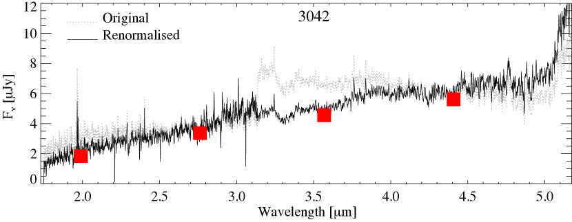
This process gives satisfactory results in most cases. Figure 1 shows the result of this procedure on 3042 which, as I’ll return to below, is a complex superposition of two galaxies which is likely the cause of the significant change in slope here. Most other galaxies show much slighter changes, but 5144 does not yield a good solution so its spectrum is used unmodified, while 4580 and 5735 do not have enough fluxes in the NIRCam catalogue to be well corrected, thus these have also been used unmodified. Further below I will also demonstrate that the measured Balmer ratios are physically meaningful and agree well with the ones measured off the re-calibrated data presented by Curti et al. (2023).
Although the process superficially works well, it has, however, a number of weaknesses: the assumption of a linear gradient with wavelength is unjustified but can be viewed as a the lowest order Taylor expansion of the correction function; the extrapolation to the reddest and bluest wavelengths is significantly uncertain, and of course the assumption of a constant spectral shape inside and outside the slit is questionable. That said, the method does improve the spectral shape quite significantly in some cases and by combining this method with an SED fitting approach and optimised photometry, some of these weaknesses can be addressed (see e.g. Tacchella et al., 2023).
It is however important to emphasise that slit-losses are unavoidable with NIRSpec and it is therefore important to develop methods to take this into account in the analysis. The suggestion from the JWST documentation is to create a forward model for the light convolved with the results for a point source. This is satisfactory if the emission lines follow the broad-band light profile, ie. have constant equivalent widths as a function of radius — this is patently not the case in some classes of low-z galaxies but is likely more trustworthy at high redshift. A systematic IFU survey of galaxies with NIRSpec will help inform this and can then be combined with forward models of the emission line distributions (e.g. Carton et al., 2017, 2018; Espejo Salcedo et al., 2022).
Alternatively one can limit the effect of slit-losses by constructing analysis methods that focus on nearby emission lines. This implicitly assumes that emission line ratios are radially constant which might be questionable and certainly is at low redshift, however in lieu of other information is not a bad assumption. This is the approach I will take, and and has also been the approach taken by all the papers using the early ERO NIRSpec data.
2.2 Redshift measurements
I present here 14 high confidence redshifts, 10 of which have already been presented in C22, one provided in Mahler et al. (2023), plus one lower confidence one, coming from the same spectrum with a high confidence redshift. The redshifts are in general obvious and have been determined by inspection. The details of the sources are given below in Table 1. The redshift of 3042b is highly uncertain and is discussed below.
There is however one point that warrants some discussion. This concerns blending/multiple sources within the aperture. Like any slit spectrograph, NIRSpec can have multiple sources fall onto the slit and thus have multiple traces. Given the depth that NIRSpec can routinely reach, this can introduce some challenges but as emphasised by Maseda et al. (2019) also opportunities. In the current dataset there are two clear cases of this: 8277 which has two sources well-separated within the slit, and 3042 which has two sources overlapping. For 8277 I have no secure redshift as I can only identify one clear line for the brightest source and none for the fainter, thus there is nothing more to be said about this here.
However, 3042 offers an interesting case study of a type that one should watch out for in future NIRSpec studies, particularly the deeper ones.
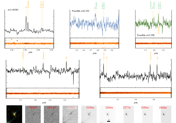
3042 is rather more complex than it might appear at first glance. There is a clear detection of the source in ACS F606W images and it continues to be detected through all NIRCAM images. However, the morphology changes dramatically through F090W and into F200W as illustrated in Figure 2. The colour image on the left on the bottom row combines the F090W, F150W, and F200W images to demonstrate the clear colour difference between the objects.
The simplest interpretation of this is that we have two sources overlapping. This has been long recognised to be a challenge with deep MUSE observations (e.g. Bacon et al., 2015; Brinchmann et al., 2017; Bacon et al., 2021) where a secure redshift can be easily found, but the assignment of this to a photometric object can be challenging, adding another axis to the classical spectroscopic confidence assessment. This is also the case here and this is likely to happen frequently in deep NIRSpec data as discussed in detail by Maseda et al. (2019), and clearly multi-band JWST/HST imaging will be paramount in dechiphering these cases.
Here the low redshift solution is clearly with , [N ii]6584, [S iii]9533, Pa- and Pa- all clearly seen although Pa- is not very well detected as it falls at a wavelength where the flux calibration is particularly problematic. [Fe ii]1.257 is also seen. My interpretation of this is that the elongated source detected in the ACS images is a lower redshift galaxy and that the redshift corresponds to this.
In contrast the source seen in F150W and redwards appears to be a higher redshift source. There are two possible redshifts for this source based on emission liens. There appears to be two lines in the spectrum at 4.7634 and 4.8828 micron, clearly seen in the 2D spectrum as can be seen in the top middle panel in Figure 2. The separation of these two lines matches well and [S ii]6717,6731 at and there are not really any other set of lines that match equally well. There are also no signs of [O iii]4959,5007. Thus the confidence for this redshift is very low. In addition there are two lines at 2.852m and 2.873m also visible in the 2D spectrum. Their separation is well fit by [N ii]6548,6584 at , but again no further supporting lines are visible so the confidence is low.
Photometric redshifts offer a possible way to distinguish between these two sources. To that effect I measured the flux of the high redshift sources in the NIRCam images, after masking out the lower redshift source. These fluxes were given to the EAZY (Brammer et al., 2008) photometric redshift code using the approach used for very faint galaxies in Brinchmann et al. (2017). The resulting is broad but rules out any redshift solutions and . While not conclusive since photo-z outliers do exist, this at least argues against the solution and I have there adopted the solution below but it is important to stress that this is highly uncertain.
3 Emission line measurements
Since one of the main goals of this paper is to compare the high-z galaxies with local counter-parts, it is preferable to use the same analysis tools used at low-z for line measurements. Thus I have adopted the platefit tool used as a basis for the MPA-JHU database444https://wwwmpa.mpa-garching.mpg.de/SDSS/DR7/ of galaxy properties (Tremonti et al., 2004a; Brinchmann et al., 2004a; Brinchmann et al., 2013). This has been well tested over two decades on surveys such as VIMOS Very Deep Survey (VVDS, e.g. Lamareille et al., 2009) and MUSE GTO (Bacon et al., 2021) and is fairly robust to spectrophotometric calibration errors and low S/N spectra.
Briefly, to estimate the continuum, platefit carries out a non-negative least squares (Lawson & Hanson, 1974) combination of Bruzual & Charlot (BC03, 2003) simple stellar population models as well as a power-law attentuation of the continuum. The best fit model is adopted and subtracted off. On the residual spectrum a smoothed continuum is constructed by taking a median smooth with box size 151 pixels and and additional boxcar smooth with a window of 51 pixels. These smooth sizes were optimized for SDSS spectra, but were found to perform satisfactorially on the JWST spectra as well. They are too wide to handle abrupt changes in the continuum between gratings due to calibration issues but as none of the main lines to be measured fall close to these edges this is not a major problem.
After also subtracting this smooth continuum, the emission lines are fit jointly in velocity space with a common velocity width and overall velocity offset, assuming that the line shape is Gaussian. As remarked above, we take the line spread function from the JWST web-site as measured pre-launch. For the MPA-JHU catalogue we tied [N ii]6548 to [N ii]6584 using a theoretical ratio of . I have updated this to use the latest NIST value of the relative ratio of and also tie the fluxes of [Ne iii]3869 and [Ne iii]3967 together using a theoretical ratio of . I do not tie the more widely separated pairs of lines [O iii]4959,5007, [S iii]9069,9533, [Fe ii]1.257,1.644 together as the residual flux calibration uncertainties could play havoc with this.
The resulting fits are acceptable but the low S/N in the continuum, if it is even detected, means that the continuum fit is poorly constrained. This does not have a strong influence on the emission line measurements but more care will be needed to obtain measurements of continuum properties. In particular the method used above, and used for the MPA-JHU catalogue, ignores the effect of a nebular continuum although the power-law attenuation accounts for this some extent. However, as shown by Cardoso et al. (2019); Pappalardo et al. (2021) this can be important precisely for these kinds of galaxies, and a more careful analaysis with e.g. FADO (Gomes & Papaderos, 2017) as has been done for extreme emission line galaxies by Breda et al. (2022), or using a modified platefit as done by Gunawardhana et al. (2020) in their analysis of the MUSE data on the Antennae, would address this. Secondly, the BC03 models are effectively based on scaled-solar abundance spectra and it is highly likely that the stars making up the stellar continuum in the highest redshift galaxies have different abundance ratios due to the different enrichment time-scales for core-collapse and type Ia supernovae, and indeed this has been argued to be of major importance also at redshift – (Strom et al., 2017; Topping et al., 2020). For the optical region of interest here, however, this should not be important.
In the lower redshift galaxies, where NIRSpec covers the rest near-IR to red optical, the platefit results are less satisfactory in part due to the lower spectral resolution of the BC03 templates used. I therefore also fit the spectrum manually using Gaussians. I adopt joint fits of Gaussians to blended, or nearly blended, lines such as C iii]1907,1909, [O ii]3726,3729, [S ii]6717,6731 and a joint triple Gaussian fit for [N ii]6548,6584 and . These Gaussian fits compare well with the platefit results but behave better in the near-IR part of the spectra so I’ll adopt those for the analysis of the galaxies.
3.1 Noise estimates
It is imperative to have good noise estimates for spectra before one measures line fluxes and in particular try to infer physical parameters from the line ratios which are more sensitive to noise. The most common approach in the papers appearing thus far has been to adopt the noise estimate from the pipeline. This appears to underestimate the true noise in the spectrum, a fact also noted by several other researchers (e.g. Rhoads et al., 2023; Trump et al., 2023).
We can quantify this by running platefit on each individual observation separately and comparing the derived fluxes. Concretely I selected all lines with S/N (a cut of 7 or 10 gives comparable results), and calculated the standardized difference,
| (2) |
where 007 and 008 refer to the individual observations and is the flux uncertainty. Under the assumption that all uncertainties are normal, this should be distributed as a unit variance normal distribution. Deviations from this can come from two sources. Firstly, the uncertainty estimates themselves are uncertain and if this is important, will be distributed as a Student’s t distribution rather than a normal — this is most easily seen in the wings of the distribution but as only 73 flux measurements were available here, this is impossible to assess. The other, and more relevant source is that underestimated uncertainties tend to inflate . For SDSS DR7 we found that this was indeed a concern (Brinchmann et al., 2013, BC13 hereafter) and here too I find that the uncertainties delivered by platefit are underestimated by a factor of 2.75 when using the pipeline reductions. A part of this is due to platefit only reporting the diagonal elements of the covariance matrix, but when applying gaussian fits manually to the lines I also find a discrepancy of a factor of 2 so this appears robust. I also find a slight bias between the two observations in that 008 is slightly brighter. Given the combination and subsequent renormalisation of the spectra, this does not matter for the results presented here.
More directly, it is notable that the root-mean-square of the spectrum in line-free regions is larger than expected from the pipeline noise spectrum so I have opted to be conservative and adopt an empirical RMS spectrum as my noise spectrum. I use a window of six pixels, calculate the standard deviation in this sliding window. reject outliers that are more than 3 deviant and recalculate the standard deviation. The results presented below are not very sensitive to this approach but the noise correction will become an issue again in section 9 below.
3.2 Sample characteristics and source description
| Object | Redshift | Confidence | Lines | Comments |
|---|---|---|---|---|
| 1917 | 3.0 | [S iii]9533, He i 1.083, | ||
| 3042 | 3.0 | , [S ii]9068,9533, He i 1.083, | Two overlapping galaxies with one invisible in F090W. The redshift Mahler et al. (2023) is for the lower redshift source. | |
| 3042b | 1.0 | Possible [N ii]6548,6584 | Highly uncertain redshift. | |
| 4580 | 5.1727 | 2.0 | [O iii]5007, . | Pointed out by Mahler et al. (2023). Only visit 008 is used to avoid problems near |
| 4590 | 3.0 | C iii]1909, [O ii]3727, to [O iii]5007 | Clear redshift but only observation 008 used | |
| 5144 | 3.0 | [O ii]3727 through to | Only exposure 007 was used. Spectrophotometric recalibration unsatisfactory. | |
| 5735 | 3.0 | [S iii]9533, He i 1.083, , | Unsatisfactory recalibration | |
| 6355 | 3.0 | [Ne iv]2423, [O ii]3727, to [O iii]5007 | [Ne iv]2423 seen in both 007 and 008. | |
| 8140 | 3.0 | [O ii]3727 through to | The combined spectrum has a feature at [Ne v]3428 but this appears only in 007. | |
| 8506 | 3.0 | , [S ii]6716,6732, [S iii]9068,9533, , He i 1.083, , | ||
| 9239 | 3.0 | , [S ii]6716,6732, [S iii]9533, , He i 1.083, , , [Fe ii]1.257 | Strong continuum so lines are hard to confirm in 2D image. | |
| 9483 | 3.0 | [S iii]9068,9533, He i 1.083, [Fe ii]1.257, , , , , , He i 2.058, H2 1-0 S(3), H2 1-0 S(2), H2 1-0 S(1) | the only galaxy with prominent H2 emission lines. | |
| 9721 | 3.0 | , [S ii]6717,6731, [S iii]9068,9533, He i 1.083, , | ||
| 9922 | 3.0 | , [O iii]4959, 5007, , [S ii]6717,6731, [S iii]9068,9533, , , , He i 1.083 | ||
| 10612 | 3.0 | [O ii]3727 through to [O iii]5007 | The highest ionization parameter galaxy |
The basic characteristics of the sources with secure redshifts are given in Table 1. Line fluxes measured for the sources are provided in the online material. The two sources 4580 and 3042b will not be included in the emission line analysis below as they have insufficient spectral information to be useful.
4 Temperatures and abundances using the empirical method
The classical way to estimate temperatures of ionized nebulae is based on the ratio of the fluxes of auroral transitions to lower lying transitions. This is a fairly straightforward technique and it was already well-established when Aller wrote his influencial book “Gaseous Nebulae” (Aller, 1956). It relies on the relatively strong temperature dependence of auroral lines relative to lower-lying levels.
The method has been widely used in nearby galaxies and star-forming regions although the faintness of auroral lines has always limited their use and they are rarely detected at high redshift (see Sanders et al., 2020, for a compilation) and have been almost exclusively focused on [O iii] detections with the recent detection of auroral [O ii]7322,7332 by Sanders et al. (2023b) the exception.
The most widely used ratio at low redshift and the most interesting one for the present sample is the [O iii]4363/[O iii]5007 ratio of doubly-ionized oxygen. This is insensitive to density over a range of densities likely to occur in star forming galaxies. For concreteness I will fix the density to where relevant. The limiting factor here is usually the detection of [O iii]4363 but also the relative flux calibration of the spectrum, including de-reddening. In view of the flux calibration issues with the spectra it is therefore desirable to find a more robust estimator both for temperatures and abundances.
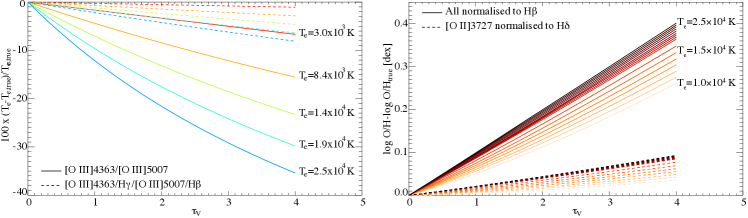
We can improve the robustness by using the double, or composite, line ratio555If the reader wants a shorthand, I offer OHOH but will refrain from using it. [O iii]4363//[O iii]5007/ instead of [O iii]4363/[O iii]5007. Double line ratios were explored by Evans & Dopita (1985) from a different angle, but they are not widely used. They do, however, offer a way to construct diagnostic diagrams that are insensitive to dust attenuation or flux calibration issues which can be helpful not only here but also when combining JWST with ground-based or other space-based facilities. I note that this ratio was also used by Trump et al. (2023) but they used it to estimate [O iii]4363/[O iii]5007 using a fixed / ratio, this however ignores the temperature sensitivity of the / ratio and as it is trivial to calculate the necessary emissivity ratios using e.g. pyneb there is no need to make this approximation.
The proposed double line ratio normalises the fluxes of the oxygen lines to their closest Balmer lines. That takes out any large-scale flux calibration issues and in fact makes the line ratio quite insensitive to dust attenuation as well. To illustrate this the left panel of Figure 3 shows the relative error we make in estimating when not accounting for dust attenuation. I have assumed here a power-law dust law with . I chose dust attenuation as one example of a spectral slope error, other functional forms like a power-law or a linear flux error give similar results and can give errors in the opposite direction as well.
The panel shows the error made using the standard ratio of [O iii]4363/[O iii]5007 as solid lines, for five different true temperatures as shown. The error here can exceed 30%. In contrast, the dashed lines show the same but now using the double line ratio [O iii]4363//[O iii]5007/. Each dashed line corresponds to the similarly coloured solid line and it is clear that the double line ratio is much more robust to calibration/dust uncertainties with an error %. This makes it particularly useful for the current situation and indeed given the potentially serious slit-loss problems for NIRSpec it would be advisable to use this approach in general. For the specific example here, an iterative solution using Balmer lines as e.g. used by Curti et al. (2023), is also insensitive. However, if instead of a smooth function with wavelength, there is an offset in flux, the iterative solution will not give correct results while the double line ratio method will continue to work.
While not of relevance here, I note in passing that a similar approach can be used for some other estimators: e.g. O iii]1661,1666 can be normalised to He ii 1640 and [O iii]5007 to He ii 4686, [S iii]9533 to and [S iii]6312 to , for instance.
The calculation of abundances follows from the calculation of temperatures. The traditional way to do this is to calculate line ratios relative to and multiply this by the ratio of the emissivity of the metal line to that of . However, there is nothing special about and this works just as well when calculating ratios to other Balmer lines. In the right panel of Figure 3, I show the difference in derived total oxygen abundance, relative to the true value as a function of the applied dust attenuation, here too the dust attenuation is just a concrete example of a flux calibration error. To construct this figure I fitted a linear relation to the ratio of the ionic abundances of and as a function for the sample of galaxies analysed in Brinchmann et al. (2008b) up to K and a constant above that. Concretely I found
| (3) |
for . I used this to assign [O ii]3727 and [O iii]5007 fluxes using the emissivities of the two transitions at the given and . In general the density will of course vary, but if the density is not known, as in the case of these high sources, it will introduce the same bias/uncertainty regardless of the method. Here it suffices to note that a change in density up or down by an order of magnitude will change the [O ii]3727/[O iii]5007 emissivity by a factor of %. For the calculation shown in the right panel of Figure 3 I used 16 values, evenly distributed between 10,000K and 25,000K. The resulting fluxes were then attenuated by dust and used to calculate . For simplicity I adopted single zone model with the temperature either derived using the standard [O iii] ratio or the double line ratio proposed above.
When using the double line ratio derived , I calculated abundances by normalising [O ii]3727 to , while for the standard approach I normalised all to . The panel shows clearly that the standard method is sensitive to flux calibration errors or errors in dust attenuation, while the proposed alternative method is more robust. It could of course be made even more robust by normalising [O ii]3727 to H() for instance, but H() is rarely detected and often strongly affected by stellar absorption so it is not clear that it will offer an improvement in practice.
The double line ratio method involves four lines, so in principle the final uncertainty will increase. In reality this is however, not a significantly concern. Firstly, [O iii]4363 is nearly always weaker than the other lines and will dominate the uncertainty on the final oxygen abundance, and if one use Balmer lines to correct for dust, all the four lines are involved thus in the end any effect on the uncertainty is very minor.
4.1 Application to the high-z galaxies
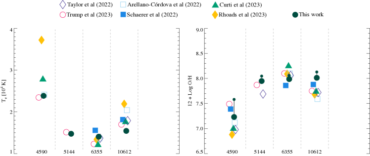
The oxygen abundances of the galaxies in the sample have been explored extensively in the literature already. For 4590, 6355, and 10612 we have five estimates (Curti et al., 2023; Trump et al., 2023; Schaerer et al., 2022; Rhoads et al., 2023; Arellano-Córdova et al., 2022) while Trump et al. (2023) also provide an estimate for 5144.
I apply the methods described above to estimate ([O iii]). To estimate the temperature of the [O ii] emitting region we have to make recourse to functional relations. To illustrate the importance of this I have used three approximations: 1. set ([O ii]) equal to ([O iii]), 2. calculate ([O ii]) using the relation proposed by Izotov et al. (2006), or 3. calculate ([O ii]) using the relation derived Pilyugin et al. (2009). I then calculate ionic abundances normalising [O ii]3727 to , using leads to changes in the abundances dex.
The resulting ([O iii]) and 12+O/H values are compared to other determinations in the literature in Figure 4. Focusing on the temperatures first, the agreement between different authors is reasonable with some outliers most notably for 4590 which has an apparently very strong [O iii]4363 line. For 8140 only Trump et al. (2023) present a temperature and abundance, I am unable to confirm their detection of [O iii]4363 and have decided to not use the direct method for this source. As we will see below, photoionization model fits prefer a rather higher abundance for this source in disagreement with Trump et al’s determination.
Turning now to the oxygen abundance plot in the right panel. This again shows decent agreement even for the extreme 4590. The effect of the ([O ii]) formula is shown as a solid and open smaller circle connected by a line to the larger, filled black circle. The larger circle corresponds to equal temperatures for the [O ii] and [O iii] zones, while the open corresponds to the Pilyugin et al relation and the small filled to the Izotov et al relation. These do not have a strong influence on the result as already noted by Curti et al. (2023) although the quadratic relation from Izotov et al. (2006) gives discrepant results for 4590, and as Rhoads et al. (2023) already noted this argues for a modification of that relation. The second point is that, like all the other publications, I have not corrected for the presence of triply ionized oxygen as this is not expected to be a significant contribution to the oxygen budget (Izotov et al., 2006; Arellano-Córdova et al., 2022; Berg et al., 2021), assuming of course that star formation is the dominant source of ionization, a point I will return to in Section 6 below.
5 Fitting the high-z sources with photo-ionization models
In order to do a systematic study of metals in a sample of galaxies, it is usually better to exploit strong lines rather than temperature sensitive lines due to their better detectability. At low redshifts it has been common to use calibrated emission line ratios as the way to get this and this has led to numerous discussions about calibration.
However calibrated emission line ratios are a very simplistic way to estimate emission line properties and it is much better to use all the data and model emission line properties using fits to photoionization models. This was first used for the SDSS in Brinchmann et al. (2004b); Tremonti et al. (2004b). It has subsequently been used more widely (Blanc et al., 2015; Vale Asari et al., 2016; Fernández et al., 2022), and more recently also combined with full-spectrum modeling (Chevallard & Charlot, 2016; Johnson et al., 2021) which also has very recently been applied to the three galaxies by Tacchella et al. (2023). It is a natural match for the data presented here since this approach can explore a wider gamut of model parameters than a calibrated emission line ratio method would do (see Maiolino & Mannucci, 2019; Kewley et al., 2019, for discussions).
For the study here I used both the original code, CL01fit, used for the SDSS studies mentioned above and last described in B13 which makes use of the Charlot & Longhetti (2001, CL01 hereafter) models, and a python re-implementation of this called PIModels which has support for multiple photoionization grids and can carry out the Bayesian analysis either using a stochastic or a gridded approach.
In either case, the codes fit a given set of lines, using a Bayesian appraoch. We calculate the log likelihood of each model, , through:
| (4) |
where is the flux in line , is a scaling-factor and corresponds to the relevant model. denotes the prior on the model parameters. For most use this high-dimensional distribution is then marginalised down to 1D or 2D probability distribution functions (PDFs) — for the most part I will focus on 1D PDFs in this paper. I will present results based on both the CL01 and Gutkin et al. (2016, G16 hereafter) models. For the CL01 models I will use the CL01fit code, while for G16 I use PIFit.
CL01fit is described in detail in B13. It is a grid-based Bayesian code and evaluates equation (4) on a grid of model parameters. This is a very fast way to do Bayesian inference and it does not raise any issues of convergence or burn-in, but it provides results on a fixed grid so can not adapt to very high signal-to-noise data. PIFit can also adopt a gridded fit, but the default is to use the MultiNest (Feroz et al., 2009) package to do nested inference through the pyMultiNest python interface (Buchner, 2016). The code interpolates between the models using either a multi-dimensional linear or the Radial Basis Function interpolation from scipy (Virtanen et al., 2020) and also fits directly for dust attenuation if dust attenuation is not one of the model parameters (as it is for CL01). For the results here I use the multi-dimensional linear interpolator as it is more robust.
The different methodologies for CL01Fit and PIFit do not significantly impact the results. However the photoionization model adopted does matter in this case. The CL01 model is based on a relatively old stellar populations code (Bruzual & Charlot, 1993) as well as an earlier version of the Cloudy photoionization code (Ferland et al., 1998). The model grid only goes down to and up to an ionization parameter of , with incomplete sampling of the model grid beyond . These were not serious limitations for application to SDSS data, but as we will see, they are more problematic when applied to the high-z data. However, it is still useful to apply this to demonstrate what inferred parameters are more sensitive to the model choice.
In contrast, the G16 models are based on up-to-date stellar population models (an updated version of the Bruzual & Charlot 2003 models) as well as version 13.03 of Cloudy (Ferland et al., 2013). They span a wider range of metallicity down to , as well as ionization parameters up to . This makes them much better suited to the present dataset and they are also used in the BEAGLE code (Chevallard & Charlot, 2016).
In either case, I run the fits using [O ii]3727, , , and [O iii]5007 as input fluxes. I have also run the fits with [Ne iii]3869 line included and it does not change the results for G16 significantly, but for the CL01 the quality of fit is reduced so I opt to exclude the line. I do not include the [O iii]4363 line because photoionization models have trouble predicting this line at a necessary accuracy (e.g. Dors et al., 2011). These are also the reasons why [Ne iii]3869 and [O iii]4363 were not used in the MPA-JHU metallicity fits. I also adopt flat priors on all parameters.
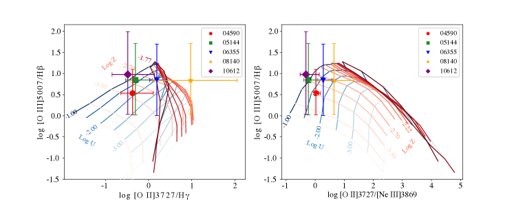
Before fitting, it is crucial to confirm, or not, that the model grid covers the space probed by the galaxies to fit. This is shown in Figure 5 where I compare a line ratio diagram for the G16 model against the objects. It is clear that most galaxies fall within the model grid although 10612 is consistently on the edge of the grid and 8140 has a somewhat discrepant [O ii]3727/ ratio albeit with a large uncertainty. The observed line ratios were not corrected for dust but the amount of dust allowed by the data is not sufficient to significantly affect these ratios since they are mostly between closely separated lines.
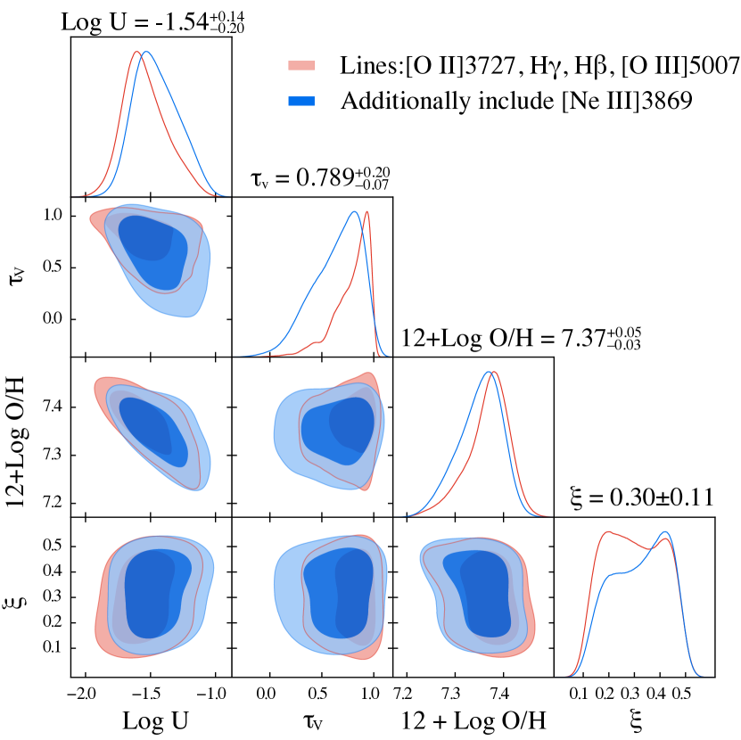
Figure 6 shows the result of running the G16 models on the data for 4590 and it evinces several aspects of photoionization model fitting that are worth keeping in mind: we see a clear correlation between dust attenuation and . In this case this is because the only lines that can constrain the ionization parameter are [O ii]3727 and [O iii]5007 and this means that both increasing the ionization parameter and increasing the dust attenuation can produce a weak [O ii]3727 line, leading to the displayed anti-correlation. This has a secondary effect on the oxygen abudance as well. There is also a correlation between and the dust-to-metal ratio, . This effect is discussed in B13 and is due to a balance between reduced gas-phase oxygen when is increased and an increased heating, see B13 for details. With the provided lines, is pretty much unconstrained, but it is an important free parameter for photoionization fits as its value is basically unconstrained at high redshift. The plot also illustrates the effect of including (blue) or not (red) the [Ne iii]3869 line in the fit. In this case, the effect is very marginal and that is also the case for 6355, 8140 and 10612, however for 5144 the inclusion of [Ne iii]3869 helps rule out high-metallicity solutions.
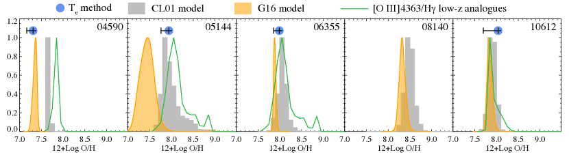
Figure 7 shows the resulting constraints on from fitting the CL01 (gray filled histogram) and G16 (orange filled histogram) models to the high- galaxies. In the case of 4590 the CL01 PDF goes right up against the low metallicity edge and the fit is overall rather poor. In contrast the other four galaxies are best fit with oxygen abundances well inside the model grid. The G16 model fits overall better but for 6355, 8140, and 10612 the resulting constraints are in very good agreement with those found using CL01.
The direct oxygen abundances calculated in section 4.1 are shown as the blue symbols with errorbars. We see that this agrees well with the G16 models. This is consistent with the findings of Dors et al. (2011) who also found that when photoionization models are considered in full, they provide results that are in good agreement with the direct method, at least at low metallicities.
Finally, the green lines show the distribution of oxygen abundances (dervied using the CL01 model) of the low- counterparts discussed in section 7. I will return to a discussion of this further below, but first it is pertinent to take a critical look at the source of ionization in the galaxies.
6 The source of ionization in the galaxies
Until now I have tacitly assumed that all galaxies in the sample have emission lines whose ionization source is dominated by star-formation. That is however, a rather strong assumption so it is important to underpin this as much as possible.
6.1 The galaxies
The source of ionization in the high-z galaxies has been extensively discussed in the literature already. It is, however, problematic to distinguish between star-bursts and AGN at low metallicities (Groves et al. (2006), see also Nakajima & Maiolino (2022)), thus it is perhaps not surprising that all conclude that the data are consistent with star formation.
Here I will instead focus on the UV lines detected in 4590 and 6355 to complement the literature studies using optical lines. Starting first with 4590, it shows C iii]1907,1909 in emission as also noted by Arellano-Córdova et al. (2022). This line is ubiquitous in AGN, but it is also commonly seen in star-forming galaxies (Stark et al., 2014; Rigby et al., 2015; Maseda et al., 2017; Ravindranath et al., 2020), in particular in those that show high intensity star bursts, so it is perhaps not surprising that it is seen here but as we will see, it does offer some extra information on the source.
Unfortunately C iii]1907,1909 is at the very blue of the spectral range and the renormalisation of flux that has been used here is not reliable at the edges. Thus I have also re-measured the flux of C iii]1907,1909 on the uncorrected spectrum. There are unfortunately no nearby lines to normalise to, thus I normalise to which is the stronger recombination line in the spectrum.
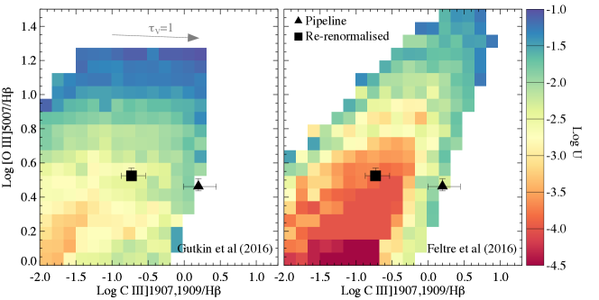
From the unmodified spectrum I find a C iii]1907,1909/ratio of , and from the corrected spectrum I find . Despite the substantial uncertainties, we can robustly conclude that the C iii]1907,1909 flux is comparable to, but somewhat lower than, that of . This is indicative of either a non-thermal ionization source or a moderate to high ionization parameter in a star-burst. I illustrate this in Figure 8. This compares the measured C iii]1907,1909/ ratios to the Gutkin et al. (2016) models for star-forming galaxies on the left, and to the Feltre et al. (2015) models for AGNs on the right. The 2D histograms show the average ionization parameter, , in each bin. Overplotted on these diagrams are the two estimates of the C iii]1907,1909/ ratio. They are clearly discrepant, implying significant systematic uncertainties, but both measurements are consistent with the models although no distinction can be made between the two sources of ionization. A reddening vector corresponding to is included in the left-hand panel. Clearly only a modest amount of dust can be accommodated before the data fall outside the model grid, in good agreement with e.g. Curti et al. (2023).
The equivalent width of C iii]1907,1909 is potentially a better discriminator of galaxy properties than these line ratios (e.g. Jaskot & Ravindranath, 2016), however the flux calibration problem and non-detection of the continuum means that this is very challenging and the data have no real constraining power. Formally, using the total F150W flux to estimate the continuum, the equivalent width is between 1 and 30Å, depending on the normalisation used and fitting method adopted. That is the entire range spanned by star forming galaxies (e.g. Rigby et al., 2015) and does not require an AGN.
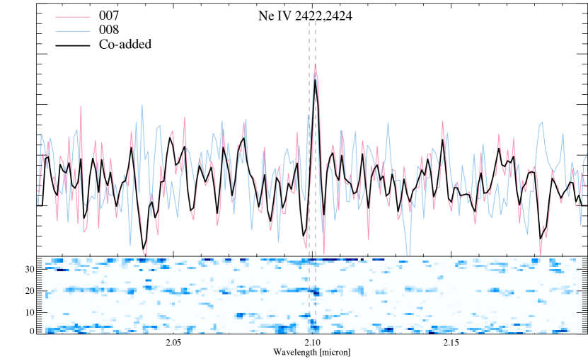
Turning now to 6355, this is an interesting case because it shows a clear detection of [Ne iv]2422,2424, as shown in Figure 9. The creation of Ne+++ requires photons with energies eV and it is therefore seen only in very energetic environments. It is commonly used as a density indicator in bright planetary nebulae (e.g. Keenan et al., 1998; Aller et al., 1999) and it is also seen regularly in AGNs (e.g. Terao et al., 2022). It is not a line associated with star forming regions, although other high ionization lines are seen in star-forming galaxies, albeit at low levels at both low and higher redshifts (e.g. Guseva et al., 2000; Shirazi & Brinchmann, 2012; Stark et al., 2014; Berg et al., 2018; Nanayakkara et al., 2019; Izotov et al., 2021; Berg et al., 2021).
The flux in the line is rather substantial although like with the C iii]1907,1909 line in 4590, there is substantial uncertainty in the flux calibration at the blue edge. Taking the measurements at face value, the flux is erg/s/cm2, which gives a [Ne iv]2422,2424/ . I am not aware of a suitable comparison sample, but I note that Terao et al. (2022) find that C iii]1907,1909 is times stronger than [Ne iv]2422,2424 in their sample of radio galaxies, and at low metallicity C iii]1907,1909 can easily be comparable to , so this ratio seems entirely reasonable.
In conclusion it seems that 6355 is hosting a narrow-line AGN in a galaxy with stellar mass at . To my knowledge this is the lowest mass galaxy to host a narrow-line AGN at these redshifts, and clearly a source that warrants a closer assessment. In particular the [Ne iv] line is weak so its significance must be considered somewhat tentative. The optical line ratios do not show clear signs of AGN activity, but since the sensitivity of [Ne iv]2422,2424 to AGN activity is much stronger than the optical lines this should not be taken as a counter-argument. In a galaxy where significant star formation is taking place, the main optical line ratios might be insensitive to a low level of AGN activity which may, however, be detectable in high ionization lines (c.f. Shirazi & Brinchmann, 2012).
Neither 5144 nor 10612 show any lines directly indicative of AGN activity but I will revisit this when comparing to local analogues below. For line ratio diagrams I point the reader to the fine presentations already in the literature (Trussler et al., 2022; Katz et al., 2023; Trump et al., 2023; Rhoads et al., 2023; Curti et al., 2023), all of whom do a great job of comparing the data to various comparison samples.
Turning now to 8140, this actually shows a strong [Ne v]3426 line in the co-added spectrum. This is however not visible in 008 and there is no He ii 4686, as well as a very low [N ii]6584/ ratio so this should also be considered a star-formation dominated source with the [Ne v]3426 detection considered spurious.
In the high-z sample we therefore appear to have 1 narrow-line AGN out of 5, which is an intriguingly high fraction but with the sample as small as it is, no firm conclusions should be drawn. It is however important to keep an eye out for these in future NIRSpec campaigns.
6.2 The galaxies
Turning next to the lower redshift galaxies, the question of ionization source is even harder to answer. There are lines that are clearly diagnostic of AGN activity in the near-IR such as the He ii 1.083 line or high-ionization S or Si lines (see e.g. Riffel et al., 2006), however these are fairly weak lines and none are seen in the spectra of the current sample galaxies. However the near-IR also has [Fe ii] lines that have long been used as shock tracers (Oliva et al., 1989; Oliva & Moorwood, 1990), as well as a rich spectrum of emission lines which can be used to gain insight in the warm neutral gas and photon-dominated regions in galaxies (e.g. Black & van Dishoeck, 1987; Kaplan et al., 2017).
| Line | 1917 | 3042 | 5735 | 8506 | ||||||||
|---|---|---|---|---|---|---|---|---|---|---|---|---|
| S/N | S/N | S/N | S/N | |||||||||
| L⊙ | L⊙ | L⊙ | L⊙ | L⊙ | L⊙ | L⊙ | L⊙ | |||||
| 12.5 | 58.8 | 27.11 | 227.2 | 2104.4 | 291.65 | |||||||
| [N ii]6584 | 5.9 | 27.4 | 14.73 | 15.0 | 139.1 | 24.69 | ||||||
| [S ii]6717 | 1.9 | 9.6 | 4.76 | 8.8 | 77.9 | 10.73 | ||||||
| [S ii]6731 | 2.2 | 11.3 | 5.72 | 6.0 | 52.4 | 7.95 | ||||||
| [S iii]9068 | 7.0 | 19.1 | 5.44 | 16.8 | 138.9 | 16.52 | ||||||
| [S iii]9533 | 1.6 | 4.9 | 13.09 | 3.8 | 14.3 | 7.61 | 29.6 | 78.1 | 17.55 | 37.3 | 299.4 | 45.63 |
| 5.5 | 43.7 | 2.63 | ||||||||||
| He i 1.083 | 1.0 | 2.8 | 5.78 | 3.0 | 9.7 | 4.51 | 21.8 | 57.5 | 10.65 | 28.6 | 225.1 | 25.51 |
| 0.3 | 0.9 | 3.46 | 1.1 | 4.2 | 1.70 | 10.3 | 81.0 | 6.14 | ||||
| [Fe ii]1.257 | 2.6 | 8.5 | 3.90 | 4.0 | 8.5 | 1.71 | 2.7 | 23.0 | 1.88 | |||
| 3.0 | 11.4 | 2.94 | 12.2 | 31.1 | 5.27 | 14.7 | 115.9 | 13.15 | ||||
| 1.4 | 3.9 | 5.13 | 12.3 | 31.9 | 5.23 | |||||||
| 0.3 | 0.7 | 3.10 | 5.2 | 13.5 | 1.74 | |||||||
| 1-0 S(3) | ||||||||||||
| 1-0 S(2) | ||||||||||||
| He i 2.058 | ||||||||||||
| 1-0 S(1) | ||||||||||||
| 9239 | 9483 | 9721 | 9922 | |||||||||
| S/N | S/N | S/N | S/N | |||||||||
| L⊙ | L⊙ | L⊙ | L⊙ | L⊙ | L⊙ | L⊙ | L⊙ | |||||
| 30.1 | 772.4 | 88.47 | 907.7 | 920.4 | 210.67 | 127.6 | 1249.2 | 384.05 | ||||
| [N ii]6584 | 13.0 | 332.1 | 44.66 | 35.4 | 35.9 | 10.53 | 4.2 | 41.0 | 16.16 | |||
| [S ii]6717 | 2.8 | 65.4 | 7.26 | 83.1 | 67.5 | 14.31 | 4.1 | 40.3 | 11.82 | |||
| [S ii]6731 | 3.7 | 82.5 | 9.07 | 61.0 | 46.6 | 11.16 | 3.9 | 37.6 | 11.22 | |||
| [S iii]9068 | 96.8 | 122.6 | 23.90 | 37.7 | 38.2 | 10.96 | 7.4 | 71.8 | 11.27 | |||
| [S iii]9533 | 7.1 | 118.8 | 10.18 | 215.5 | 273.0 | 50.58 | 56.4 | 55.5 | 12.60 | 16.1 | 153.9 | 22.98 |
| 1.5 | 25.5 | 2.34 | 2.6 | 25.3 | 3.86 | |||||||
| He i 1.083 | 4.0 | 64.1 | 5.99 | 107.4 | 132.2 | 24.31 | 45.4 | 46.0 | 5.17 | 10.8 | 106.8 | 15.06 |
| 2.2 | 39.6 | 4.98 | 49.8 | 64.9 | 12.20 | 31.2 | 31.6 | 1.49 | 3.8 | 34.2 | 5.41 | |
| [Fe ii]1.257 | 2.2 | 37.1 | 3.49 | 68.3 | 83.0 | 14.34 | ||||||
| 5.6 | 86.0 | 9.48 | 134.5 | 171.0 | 28.81 | 20.9 | 21.2 | 3.33 | 4.2 | 42.1 | 5.14 | |
| 377.1 | 478.0 | 43.17 | ||||||||||
| 1-0 S(3) | 28.8 | 35.7 | 3.34 | |||||||||
| 1-0 S(2) | 16.7 | 18.6 | 1.69 | |||||||||
| He i 2.058 | 22.2 | 28.1 | 1.74 | |||||||||
| 1-0 S(1) | 22.1 | 26.5 | 2.82 | |||||||||
| 28.0 | 39.5 | 3.04 | ||||||||||
Starting with the more classical optical line ratios, 3042 has a [N ii]6584/ line ratio above that normally seen in star forming regions, but in contrast the dereddened [S iii]9533/ ratio () matches very well the values found in metal rich H ii regions locally (e.g. Bresolin et al., 2004), where I assumed an intrinsic using atomic parameters from NIST. While no very firm conclusion can be made from this alone, the most likely conclusion appears to be that there is a contribution of non-star formation activity in this source to boost the [N ii]6584 flux.
Of the other galaxies, 9239 has [S ii]6717,6731/ which places it in the middle of the distribution of this ratio for star-forming galaxies (e.g. Kewley & Dopita, 2002; Brinchmann et al., 2008a), and its [S iii]9533/ ratio is also consistent with star formation.
Turning now to the more interesting [Fe ii] lines, the only regularly detected line is [Fe ii]1.257 which we find in 3042, 9239, and 9483. This line is seen in nearby starbursts (e.g. Vanzi et al., 2008; Cresci et al., 2010; Izotov & Thuan, 2016) but it is typically quite weak at a few percent of . The exception is in shock dominated regions or in the narrow-line regions of AGN (e.g. van der Werf et al., 1993; Alonso-Herrero et al., 1997; Mouri et al., 2000; Rosenberg et al., 2012) where it can reach much higher values.
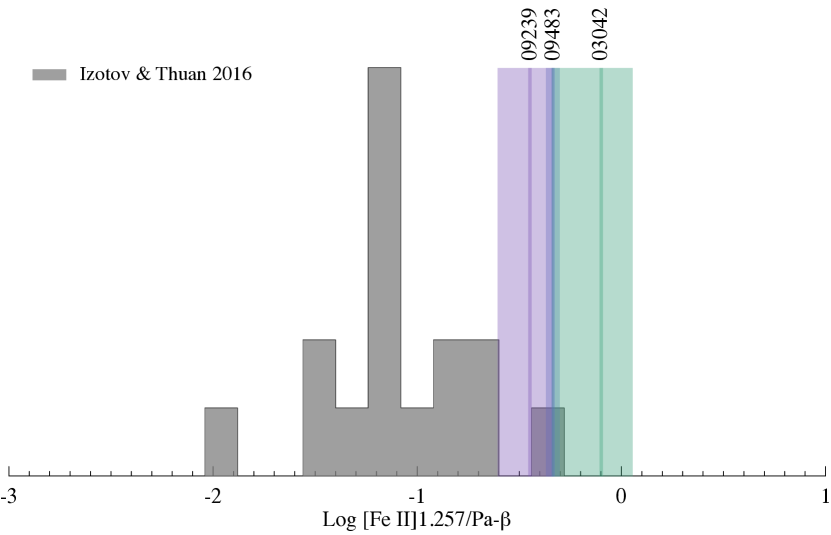
Indeed, the [Fe ii] lines seen in these spectra are all much too bright to be caused by star formation, and much brighter than normally seen in nearby starburst galaxies. To demonstrate this, Figure 10 compares the measured [Fe ii]1.257/ ratios in the three galaxies against the ratios measured in 24 nearby BCDs and H ii regions by Izotov & Thuan (2016). It is clear that with the exception of the H ii region J1038+5330 in NGC 3310 noted by Izotov & Thuan, all the low-z galaxies have much weaker [Fe ii] emission.
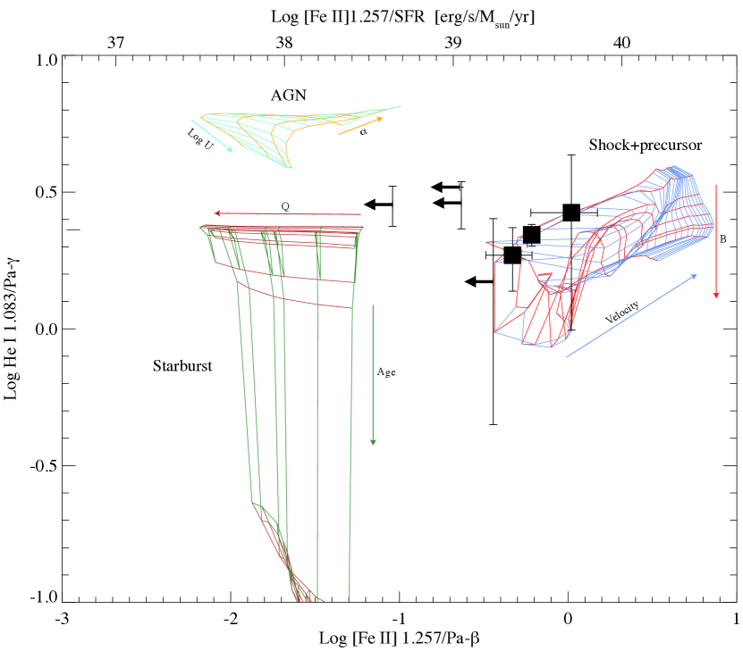
We can contrast this to models more directly because [Fe ii]1.257 is fairly close to and if I combine this with He i 1.083/ which again is a ratio of nearby lines, I get figure 11.
This figure shows the data for the three galaxies with detected [Fe ii]1.257 as the solid squares with error-bars. The other galaxies are shown at the upper limit for the [Fe ii]1.257 flux. I contrast this against three different model libraries. I have taken a single example grid from three libraries in the literature: the high-massloss starburst grid with from Levesque et al. (2010), a solar metallicity dusty AGN model grid from Groves et al. (2004a, b), and a solar metallicity shock model grid from Allen et al. (2008) where I used the shock+precursor grid. All models were obtained through the itera code by Groves & Allen (2010).
The immediate observation we can make is that the three SMACS galaxies with clearly detected [Fe ii]1.257 all fall clearly in the shock dominated region. They lie towards the high -field, low velocity region of the shown grid. In reality these galaxies are likely to have a mix of shocks, star-formation and AGN contributing to their emission lines and a more detailed modeling would be required to disentangle these and the present data are not of sufficient quality to warrant this. Furthermore, for some of these galaxies the aperture corrections are substantial, this is shown in Table 2 which provides line luminosities on spectra normalised to aperture fluxes and total fluxes. That said, however, it will be of considerable interest to understand these “shock-dominated” galaxies in more detail and to understand how they fit into the overall population of galaxies at these redshifts (see also Reddy et al., 2023). It would also be very desirable to have additional diagnostic ratios to further understand the nature of these sources, but only 3042 has some qualitatively different lines, in [N ii]6583, [S iii]9533, and and those are not strongly diagnostic of shock activity (Allen et al., 2008). Instead Allen et al. (2008) recommended UV and UV-optical diagnostics such as C iii]1909/C ii]2326 and [Ne iii]3869/[Ne v]3426, neither of which are available for our galaxies but which conceivably could be obtained for galaxies with deep ground-based observations.
The final set of lines of key interest are the lines. These originate in the cooler medium outside the H ii regions and as such provide very complementary information to lines coming from hotter regions of the ISM. In the present sample only 9483 shows strong lines and even then only three: 1-0 S(3), 1-0 S(2) and 1-0 S(1). 1-0 S(3) is contaminated by He i 1.955, leaving only the 1-0 S(2)/ 1-0 S(1) ratio as a diagnostic. This ratio has a value of which is comparable to the values found by Izotov & Thuan (2016) for nearby star-forming galaxies and regions (0.3–0.8) and the value of 0.28 found for the Orion Bar by Kaplan et al. (2017). Since we saw above that 9483 has a significant contribution of shocks to its [Fe ii]1.257 line flux, one might expect that the line ratios should approach that corresponding to a thermal distribution. Unfortunately the detected lines are not very diagnostic for this as the models for thermal and fluorescent emission in Black & van Dishoeck (1987) span this range, with a preference for a lower value for thermal distributions and somewhat higher for fluorescent emission but in either case consistent with the observed line ratio. Future observations will surely provide much more information on this and open up the diagnostic potential of lines for galaxies out to with NIRSpec.
7 Comparison to local galaxies
As discussed in the introduction, analogues of high-z galaxies in the local Universe have been sought after for a long time, and naturally the first papers looking at these NIRSpec data have discussed extensively their properties in the context of nearby galaxies. Thus Schaerer et al. (2022) compared the sample of extreme line-emitters from Izotov et al. (2014) and galaxies from the Low-Z Lyman Continuum Survey (LzLCS, Flury et al., 2022) to the NIRSpec sample, finding considerable correspondences. Rhoads et al. (2023) compared the NIRSpec sample to nearby Green Pea galaxies (e.g. Cardamone et al., 2009; Jaskot & Oey, 2013), specifically from the sample defined in Jiang et al. (2019) and Yang et al. (2019). A mixture of those approaches was taken by Trump et al. (2023) who compared both to Green Peas from Brunker et al. (2020) but also to extreme line emitters from Pérez-Montero et al. (2021). A similar approach was taken by Katz et al. (2023) who compared against compact galaxies of various colour (Yang et al., 2017a, b), as well as low-metallicity galaxies (Izotov et al., 2019) and exteme line-emitters (Amorín et al., 2015). With small variations, all these authors and comparisons find that there are galaxies in the nearby Universe that are broadly similar to the NIRSpec sample, although exactly how similar is open to some discussion.
What is noticeable is that these studies all limit themselves to star forming galaxies, thus there is an a priori assumption that the ionization source in these galaxies must be star formation. This might very well be correct and it is not an unreasonable assumption, but as we saw above, 6355 appears to have an AGN contribution and it is notoriously difficult to distinguish between AGN and star formation as ionization source at low metallicity. Thus here I take a slightly different approach. I will not start with a particular sample but rather I will ask: what galaxies in the local Universe have similar emission line properties to the NIRSpec sample and what are the properties of this local sample?
Since I am interested in excitation properties, I will focus on line ratios and ignore extrinsic quantities like size or mass. Specifically I always require the [O iii]5007/ ratio to match the NIRSpec sample within 1, and then define two samples: the [O iii]4363/ counterparts and the [Ne iii]3869/[O ii]3727 counterparts. I will base myself on the SDSS DR7 sample used in B13 and only use galaxies with S/N in all relevant lines. With these preambles we find the following results:
-
•
4590: there are 13 galaxies with [O iii]4363/ within 1. 6 of these are AGN, while 4 are star-forming, 2 composite and one unclassified. The [Ne iii]3869/[O ii]3727 ratio gives a similar result with 2/3 AGNs and 1/3 star-forming.
-
•
5144: there are 192 galaxies with [O iii]4363/ within 1 of 5144. 73% of these are star-forming and all but 2 of the remainder are classified as AGN. The [Ne iii]3869/[O ii]3727 ratio is matched by no galaxies in the SDSS within 1.
-
•
6355: there are 155 galaxies that are close to the [O iii]4363/ ratio. Of these 76% are star-forming while the remainder are almost all AGN. When considering [Ne iii]3869/[O ii]3727 only 40 galaxies are within 1 of the NIRSpec data. Out of these 55% are AGN, 2 unclassified, and the rest star-forming.
-
•
8140: as I do not consider this to have [O iii]4363 I do not consider this ratio, but for the [Ne iii]3869/[O ii]3727 ratio a total of 371 galaxies in the SDSS fall within 1. These are composed of 15% star-forming and 82% AGN.
-
•
10612: there are 172 SDSS galaxies with [O iii]4363/ within 1 of the NIRSpec data. Out of these only 3 are classed as star-forming, with the remainder all falling in the AGN part of the BPT diagram. There are only two galaxies that have [Ne iii]3869/[O ii]3727 within 1 of the NIRSpec data, one AGN, one star-forming galaxy.
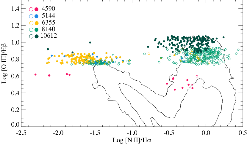
These results are summarised in Figure 12 where filled disks show the [O iii]4363/ analogues while the open symbols the [Ne iii]3869/[O ii]3727 ones. It is evident that based on the observed line ratios the local counter-parts will fall in two regions: they are either low-Z star-forming galaxies (or low-Z AGNs we should not forget), or clear AGN. Taken at face value this suggests that we should at least take the assumption that all these are powered by star formation with a grain of salt, although one should not over-interpret the results of the local sample either. In particular the 10612 which is easily the most extreme galaxy in the sample, must be questioned as to its ionization source as also pointed out by Schaerer et al. (2022).
For the [O iii]4363/ analogues I have also co-added the PDFs of all their derived parameters from the fits described in Brinchmann et al. (2013). In the following section (see also Figure 7), I will compare the resulting distributions to the high-z galaxies. This is only possible for star-forming galaxies, thus when reading the following section it is important to keep in mind that there is a possibility that several of these sources have a contribution of an AGN to their line fluxes which will make some of the following results less conclusive.
8 Gas-phase properties of the galaxies
| Quantity | 4590 | 5144 | 6355 | 8140 | 10612 |
|---|---|---|---|---|---|
| (CL01) | |||||
| (G16) | |||||
| Log U (CL01) | |||||
| Log U (G16) | |||||
| (CL01) | |||||
| (G16)) | |||||
| Log SFR (CL01) | |||||
| Log SFR (G16) | |||||
| [yrs] (CL01) |
Returning now to the CL01 and G16 photoionization model fits to the data, Figure 13 shows multiple fit parameters for the five high- galaxies. The first row shows the ionization parameter for each galaxy and here we immediately see one of the limitations of the CL01 grid: it does not go to sufficiently high ionization parameters and the PDFs are pushed up towards the edge. For those galaxies for which this is noticeable, 5144 and 10612 in particular, this puts the other results into question although we saw in Figure 6 that is relatively independent of other parameters in the fit. I do not show the analogue sample in this row as the CL01 model is such a poor match in this respect.
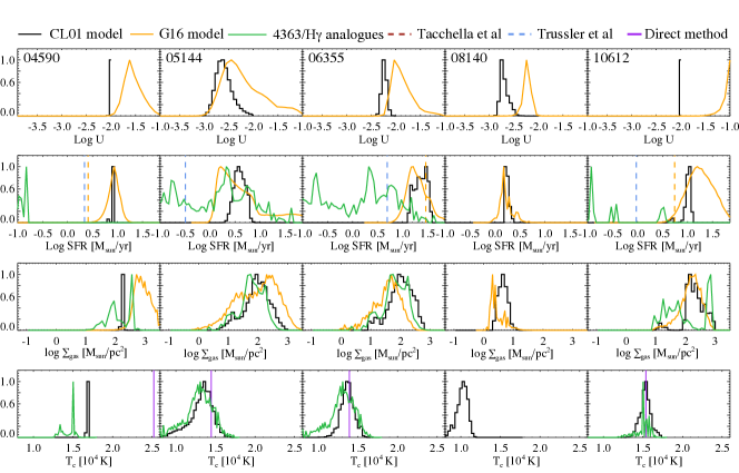
The second row shows the star formation rate, derived from the scaling parameter in equation (4). The star formation rates inferred from the emission lines are corrected for lensing using the same values as Trussler et al. (2022) which are taken from Pascale et al. (2022). The dashed blue lines show the Star Formation Rate (SFR) estimates from the photometry presented in Trussler et al. (2022) (who did not provide a value for 8140) and the dashed burgundy lines those presented by Tacchella et al. (2023) adjusted to use the same magnification values as Trussler et al. (2022). They all agree to within a factor of 3, but often better — indeed the agreement with Tacchella et al. (2023) is considerably better than this despite very different methodologies. However the spectroscopic estimates should be considered to have a substantial systematic uncertainty due to the uncertain flux calibration. The SFR distributions for the local analogues show a very large spread which is not surprising as the matching was done ignoring all extrinstic quantities.
The third row shows an estimate of the surface gas mass density of the galaxies following the methodology of B13 (see that reference for details). The results are interesting in that they prefer high surface mass densities for all the high SFR sources. These gas estimates are in reasonable agreement between CL01 and G16 when the CL01 models are adequate fits, and it is also clear that the local analogues have similar gas properties to the galaxies. If we assume that the emission lines come from a region with area which is not entirely out of question given the small sizes, we find depletion times of (see Table 3). This is short but very similar to the values found for starbursting galaxies in B13, and it is in good agreement with the conclusion of Tacchella et al. (2023) that these appear to be rapidly accreting galaxies.
The final row shows electron temperature estimates from the models, compared to those obtained from the direct method. The values from the CL01 fits are averages over the Strömgren sphere which in general leads to lower temperatures than from [O iii]4363/[O iii]5007 but for both 6355 and 10612, the CL01 fits give temperatures in good agreement with the direct method. While this could be interpreted as evidence for very hot ionized gas where the [O iii]4363/[O iii]5007 provides a good estimate of the mean temperature, the fact that the CL01 model is a poor fit for both of these argues against any strong conclusion but it does highlight the usefulness of using photo-ionization models to estimate electron temperatures as well. In all but 4590 the CL01 fit to the low- analogues also results in temperatures similar to the high- galaxies.
These quantities, including the depletion time are all given in Table 3 for the five galaxies with sufficient lines. 4580 does not have sufficient lines for a photoionization model fit to be useful. It is also important to keep in mind that the errors given in the table do not include systematic uncertainties which given the calibration uncertainties could be substantial.
9 Discussion
Despite the lingering calibration issues, these data are demonstrating how ground-breaking NIRSpec will be for the study of ionized gas in galaxies.
The galaxies are showing a surprising amount of shock excited gas signaled by an elevated [Fe ii]1.257 emission. In the local Universe this is not seen in low-mass star-bursts (Izotov & Thuan, 2016) and regions where [Fe ii] is significantly enhanced tends to be associated with shocked regions or AGNs. The shocks in this case is usually assumed to be associated with supernova remnants (SNRs, Greenhouse et al., 1991; Alonso-Herrero et al., 2003; Rosenberg et al., 2012). Bruursema et al. (2014) used this to search for SNRs in NGC 6946 and found a typical luminosity per SNR of . It should be noted that there is a spread of almost an order of magnitude in this luminosity and other studies find different mean values, but if we adopt the Bruursema et al. value, we find that the [Fe ii]1.257 luminosity of our three sources corresponds to 2–3 [Fe ii]-luminous SNR. Thus, if the [Fe ii]1.257 all comes from SNR, we can estimate a supernova rate , assuming a typical life-time for the bright radiative shocks of (Vink, 2020). This is not an unreasonable rate of star formation, thus this presents a plausible scenario for the brightness of the [Fe ii] lines. However it does not address the question of why other galaxies (1917, 5735, 8506, 9721, 9922) show no sign of [Fe ii]1.257 despite also having bright Paschen lines. Indeed in figure 11 the top -axis shows the [Fe ii]1.257 luminosity per SFR, and as can be seen, this varies strongly between the galaxies
Turning now to the high redshift galaixes, several of the papers on these galaxies have commented on the high value of [O iii]4363/ or [O iii]4363/[O iii]5007 in 4590. I have avoided this until now because I do not feel there is much reason to worry to much about this. Firstly, the [O iii]4363 line is weak, only detected at 3–4 depending on the noise estimate adopted. Secondly, the other lines in the galaxy do not show particularly extreme properties thus there is no clear reason to think that this is anything but a statistical fluke. Indeed the fits to the G16 model above predicts a [O iii]4363 flux somewhat lower than that observed which would make the galaxy much more normal.
In contrast, 6355 appears to show [Ne iv]2422,2424 in emission and is most likely a narrow-line AGN, while 10612 has an ionization parameter which is normally the regime occupied by AGNs. One might object that He ii 4686 is not seen, but the expected flux given the strong-line fluxes is below erg/s/cm-2 (the G16 model predicts erg/s/cm-2 for an extreme star-forming model) which is below the detection threshold of the data. This then argues for potentially at least two out of the five high- galaxies being affected by AGN activity.
It is also clear that the low- analogues are showing intrinsic properties very well matched to the high- galaxies and this appears to justify the long-standing quest to carefully characterise these to contrast to high- galaxies. It also allows us to examine a potential bias that might affect all NIRSpec studies of high- galaxies.
9.1 Selection of galaxies and biases in the mass-metallicity relation
Several papers (e.g. Schaerer et al., 2022; Curti et al., 2023) have already tried to assess the evolution of the mass-metallicity (MZ) relation with redshift by comparing the JWST SMACS results to (Tremonti et al., 2004b; Yates et al., 2012; Andrews & Martini, 2013; Telford et al., 2016; Curti et al., 2020) and results (e.g. Sanders et al., 2020). With only three galaxies, selected in a somewhat haphazard manner and still substantial uncertainties in the stellar mass estimates (e.g. Schaerer et al., 2022; Tacchella et al., 2023; Carnall et al., 2023) this is of course preliminary. That aside, these studies do demonstrate the potential of future, larger, JWST studies to make real progress here.
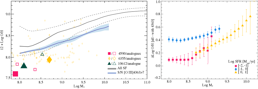
There are many potential biases when constructing the MZ relation and this has been discussed in the literature (see Telford et al., 2016; Cresci et al., 2019), but one important potential bias for the current scenario is the requirement to have a detected [O iii]4363. It is possible to make recourse to the local sample again to understand how this comes about. Note that the bias I discuss here also applies to the mass-metallicity-SFR (Mannucci et al., 2010; Lara-López et al., 2010).
Since [O iii]4363 is exponentially sensitive to the temperature of the ionized gas, requiring the detection of this line means that you will always get a sample of the lowest metallicity galaxies at each mass. This bias was already commented on indirectly by Sanders et al. (2020) who focused their discussion on the construction of calibration relations and the SFR distributions of the samples used to construct these. The bias is however more directly affecting the MZ relationship as it becomes more pronounced as one moves to higher masses (higher mean metallicities).
To illustrate this, the left panel of Figure 14 shows the MZ plane for the SDSS DR7 and the effect of selection on [O iii]4363 detectability. The black line shows the median trend for all SF galaxies from the SDSS DR7 sample of B13 and the dashed lines the 68% spread around this with the grey shading showing the 68% uncertainty on the median as determined from bootstrap resampling including Monte Carlo sampling of the uncertainties on and . To reduce aperture correction effects, I have limited my sample to have and a half-light diameter no more than 3 times the fibre diameter of the SDSS, but I have not removed failed deblends as done by e.g. Andrews & Martini (2013); the conclusions here are not significantly affected by the details of these criteria.
The dark blue line with light blue shading shows the same, but now requiring a in [O iii]4363 with the shading indicating the 68% uncertainty on the median. It is clear that applying this criterion leads to a median trend that is offset by 0.1–0.25 dex and with a flatter slope than the main sample. Thus one would conclude that this sample is significantly offset — despite using the same stellar mass and metallicity indicators here.
One might rightly object that the SFR distribution of the two samples are different, so in the right panel I show the difference between the main sample and the sample requiring a in [O iii]4363 as a function of mass divided in three bins of as measured within the fibre, as indicated in the legend. The errorbars correspond to uncertainties on the median, the 68% spread is much larger. It is clear that there is a systematic trend with mass and it is even larger than when not controlling for SFR. The differences between the different SFR bins are small, but systematic: at low SFR the sample of all versus that with [O iii]4363 are nearly coincident so very little difference is seen. At somewhat higher SFRs we have the largest difference in sample and at very high SFR and low we again have very large overlap between the samples. One should, however, be cautious with overinterpreting this figure, however, as the SDSS is not complete below and the sample of galaxies with [O iii]4363 does include galaxies that were not targetted as such. However the basic lesson appears robust: constructing MZ relations based on direct method metallicities requires very careful assessment of selection biases when comparing samples.
To put this in the context of the high- galaxies, I have also inserted these (filled symbols) with their [O iii]4363/ star-forming analogues (open symbols) in the figure. The squares show 4590 and its analogues, the diamonds 6355 and its analogues and the triangles 10612 and its sole star-forming analogues. For this plot I have used stellar masses from Tacchella et al. (2023) and the CL01 model to estimate metallicities in order to compare directly to SDSS DR7, however a very similar picture is found using the G16 model.
Does this mean that this bias will also apply at high redshift? This is one of the questions that upcoming JWST surveys with NIRSpec will be able to tell us — it depends on the spread in metallicity at a given mass. If this is very small at high redshift, then a sample defined to have detected [O iii]4363 will provide a good measure of the mean metallicity, but if there is substantial scatter then direct method metallicities might result in a significantly biased MZ relation, including most likely an incorrect slope.
Since we saw above that photoionization modelling gives oxygen abundances in good agreement with the direct method, as long as the models span a sufficiently large range in physical parameters, a viable way to combat these potential biases is to use photoinization models to estimate oxygen abundances for all galaxies instead — using [O iii]4363 to validate the results on a case-by-case basis.
10 Conclusions
In the preceding I have presented three new redshifts, all at , bringing the total number of secure redshifts for these NIRSpec observations in the SMACS 0723 field to 14. I highlighted the usefulness of modifying the methodology for direct temperature estimates to use the double line ratio [O iii]4363//[O iii]5007/. Doing so reduces senstivity to flux calibration or dust attenuation uncertainties by a factor of . If in addition the ionic abundance determinations are referenced to nearby hydrogen lines, one can strongly reduce effect of flux calibration uncertainties or unknown reddening on oxygen abundance determinations. Given the unavoidable wavelength-dependent slit losses with NIRSpec this modification of the methodology is likely to be beneficial for future high- abundance studies.
I also find that 6355 shows a fairly clear [Ne iv]2422,2424 line which I argue is evidence for this being a narrow-line AGN. The existence of one such high-z, low-mass AGN is interesting but larger samples are necessary before any implications for the process of reionization become clear. However it is notable that 10612 is showing line ratios that at low- are commonly seen in AGN, which coupled to an ionization parameter that reaches the model boundary at , suggests that this galaxy also might harbour an AGN, thus one must interpret these results with some caution.
The lower redshift galaxies also seem to be rather active with three galaxies showing very strong [Fe ii]1.257/ relative to what star-forming galaxies at is showing. These galaxies have emission spectra that can be explained nearly fully by shock models and one possible explanation is that they have a particularly high number of supernova remnants. Further data are needed to fully understand why some galaxies show very strong [Fe ii] lines and others not, while having comparable Paschen lines, but clearly aperture corrections will play an important role here.
I also presented modelling of the high- galaxies using photoionization models and show that these models result in inferred oxygen abundances in good agreement with those found using the direct method. Thus Bayesian modeling using photoionization model grids is a viable way to estimate the physcial conditions in galaxies also in conditions where [O iii]4363 is not detected, thus making for a better technique for large samples, reducing complex selection effects.
Finally, I showed that selecting samples based on the presence of [O iii]4363 has the potential to significantly bias determinations of the mass-metallicity relation and that a careful assessment of selection effects must be made in this case and I argued that it might be better to base oneself on Bayesian photoionization modeling of the strong lines than to use temperature sensitive lines as the main oxygen abundance estimation technique when doing statistical studies such as of the mass-metallicity relation.
Acknowledgements
Firstly, I would like to thank the JWST commissioning team for providing these data early and giving us all a taster of what JWST will bring in the coming years. I thank Michael Maseda, Themiya Nanayakkara, Madusha Gunawardhana, Leindert Boogaard, Roberto Maiolino for very helpful comments on an earlier version of the text. The research presented here was supported by Fundação para a Ciência e a Tecnologia (FCT) through research grants UIDB/04434/2020 and UIDP/04434/2020. JB acknowledges financial support from the Fundação para a Ciência e a Tecnologia (FCT) through national funds PTDC/FIS-AST/4862/2020 and work contract 2020.03379.CEECIND.
The research here made use of the IDL666https://www.l3harrisgeospatial.com/Software-Technology/IDL, Python777https://python.org, in particular numpy (Harris et al., 2020) and Astropy,888http://www.astropy.org a community-developed core Python package for Astronomy (Astropy Collaboration et al., 2013, 2018), Perl999https://www.perl.org, and Julia101010https://julialang.org/ (Bezanson et al., 2017) programming languages. I also made use of the DS9 (Joye & Mandel, 2003) image visualization program.
Data Availability
The analysis presented here is based on the publicly available L3 data products provided in the Barbara A. Mikulski Archive for Space Telescopes (MAST), as well as datasets provided in the literature.
Tables with line fluxes are available from https://github.com/jbrinchmann/JWST_SMACS. The PIFit code is currently in pre-beta and is available upon reasonable request but will be publicly released in the near future. The CL01Fit and platefit IDL codes are available upon reasonable request, but a Python version of platefit will released with Bacon et al (submitted).
References
- Allen et al. (2008) Allen M. G., Groves B. A., Dopita M. A., Sutherland R. S., Kewley L. J., 2008, The Astrophysical Journal Supplement Series, 178, 20
- Aller (1956) Aller L. H., 1956, Gaseous Nebulae. Chapman & Hall, London
- Aller et al. (1999) Aller L. H., Hung S., Feibelman W. A., 1999, Proceedings of the National Academy of Science, 96, 5366
- Alonso-Herrero et al. (1997) Alonso-Herrero A., Rieke M. J., Rieke G. H., Ruiz M., 1997, The Astrophysical Journal, 482, 747
- Alonso-Herrero et al. (2003) Alonso-Herrero A., Rieke G. H., Rieke M. J., Kelly D. M., 2003, The Astronomical Journal, 125, 1210
- Amorín et al. (2015) Amorín R., et al., 2015, Astronomy & Astrophysics, Volume 578, A105, 578, A105
- Andrews & Martini (2013) Andrews B. H., Martini P., 2013, The Astrophysical Journal, 765, 140
- Arellano-Córdova et al. (2022) Arellano-Córdova K. Z., et al., 2022, The Astrophysical Journal, 940, L23
- Astropy Collaboration et al. (2013) Astropy Collaboration et al., 2013, A&A, 558, A33
- Astropy Collaboration et al. (2018) Astropy Collaboration et al., 2018, AJ, 156, 123
- Bacon et al. (2015) Bacon R., et al., 2015, Astronomy and Astrophysics, 575, 75
- Bacon et al. (2021) Bacon R., et al., 2021, Astronomy & Astrophysics, 647
- Beichman et al. (2012) Beichman C. A., Rieke M., Eisenstein D., Greene T. P., Krist J., McCarthy D., Meyer M., Stansberry J., 2012, in Science opportunities with the near-{IR} camera ({NIRCam}) on the {James} {Webb} {Space} {Telescope} ({JWST}). p. 84422N, doi:10.1117/12.925447, https://ui.adsabs.harvard.edu/abs/2012SPIE.8442E..2NB
- Berg et al. (2018) Berg D. A., Erb D. K., Auger M. W., Pettini M., Brammer G. B., 2018, The Astrophysical Journal, 859, 164
- Berg et al. (2021) Berg D. A., Chisholm J., Erb D. K., Skillman E. D., Pogge R. W., Olivier G. M., 2021, The Astrophysical Journal, 922, 170
- Berg et al. (2022) Berg D. A., et al., 2022, The Astrophysical Journal Supplement Series, 261, 31
- Bertin & Arnouts (1996) Bertin E., Arnouts S., 1996, Astronomy and Astrophysics Supplement Series, 117, 393
- Bezanson et al. (2017) Bezanson J., Edelman A., Karpinski S., Shah V. B., 2017, SIAM Review, 59, 65
- Bian et al. (2016) Bian F., Kewley L. J., Dopita M. A., Juneau S., 2016, The Astrophysical Journal, 822, 62
- Black & van Dishoeck (1987) Black J. H., van Dishoeck E. F., 1987, The Astrophysical Journal, 322, 412
- Blanc et al. (2015) Blanc G. A., Kewley L., Vogt F. P. A., Dopita M. A., 2015, The Astrophysical Journal, 798, 99
- Boucaud et al. (2016) Boucaud A., Bocchio M., Abergel A., Orieux F., Dole H., Hadj-Youcef M. A., 2016, Astronomy & Astrophysics, 596, A63
- Brammer et al. (2008) Brammer G. B., van Dokkum P. G., Coppi P., 2008, The Astrophysical Journal, 686
- Breda et al. (2022) Breda I., et al., 2022, Astronomy & Astrophysics, 663, A29
- Bresolin et al. (2004) Bresolin F., Garnett D. R., Kennicutt Jr. R. C., 2004, The Astrophysical Journal, 615, 228
- Brinchmann et al. (2004b) Brinchmann J., Charlot S., White S. D. M., Tremonti C., Kauffmann G., Heckman T., Brinkmann J., 2004b, Monthly Notices of the Royal Astronomical Society, 351, 1151
- Brinchmann et al. (2004a) Brinchmann J., Charlot S., White S. D. M., Tremonti C., Kauffmann G., Heckman T., Brinkmann J., 2004a, MNRAS, 351, 1151
- Brinchmann et al. (2008a) Brinchmann J., Pettini M., Charlot S., 2008a, MNRAS, 385, 769
- Brinchmann et al. (2008b) Brinchmann J., Kunth D., Durret F., 2008b, A&A, 485, 657
- Brinchmann et al. (2013) Brinchmann J., Charlot S., Kauffmann G., Heckman T., White S. D. M., Tremonti C., 2013, Monthly Notices of the Royal Astronomical Society, 432, 2112
- Brinchmann et al. (2017) Brinchmann J., et al., 2017, Astronomy and Astrophysics, 608, A3
- Brunker et al. (2020) Brunker S. W., Salzer J. J., Janowiecki S., Finn R. A., Helou G., 2020, The Astrophysical Journal, 898, 68
- Bruursema et al. (2014) Bruursema J., Meixner M., Long K. S., Otsuka M., 2014, The Astronomical Journal, 148, 41
- Bruzual & Charlot (1993) Bruzual G., Charlot S., 1993, ApJ, 405, 538
- Bruzual & Charlot (2003) Bruzual G., Charlot S., 2003, MNRAS, 344, 1000
- Buchner (2016) Buchner J., 2016, Astrophysics Source Code Library, p. ascl:1606.005
- Bunker et al. (2023) Bunker A. J., et al., 2023, JADES NIRSpec Spectroscopy of GN-z11: Lyman-$\alpha$ emission and possible enhanced nitrogen abundance in a $z=10.60$ luminous galaxy, doi:10.48550/arXiv.2302.07256, http://arxiv.org/abs/2302.07256
- Cameron et al. (2023) Cameron A. J., et al., 2023, JADES: Probing interstellar medium conditions at $z\sim5.5-9.5$ with ultra-deep JWST/NIRSpec spectroscopy, doi:10.48550/arXiv.2302.04298, http://arxiv.org/abs/2302.04298
- Cardamone et al. (2009) Cardamone C., et al., 2009, Monthly Notices of the Royal Astronomical Society, 399, 1191
- Cardoso et al. (2019) Cardoso L. S. M., Gomes J. M., Papaderos P., 2019, Astronomy & Astrophysics, 622, A56
- Carnall et al. (2023) Carnall A. C., et al., 2023, Monthly Notices of the Royal Astronomical Society, 518, L45
- Carton et al. (2017) Carton D., et al., 2017, Monthly Notices of the Royal Astronomical Society, 468, 2140
- Carton et al. (2018) Carton D., et al., 2018, Monthly Notices of the Royal Astronomical Society, 478, 4293
- Charlot & Longhetti (2001) Charlot S., Longhetti M., 2001, MNRAS, 323, 887
- Chevallard & Charlot (2016) Chevallard J., Charlot S., 2016, Monthly Notices of the Royal Astronomical Society, 462, 1415
- Coe et al. (2019) Coe D., et al., 2019, The Astrophysical Journal, 884, 85
- Cresci et al. (2010) Cresci G., Vanzi L., Sauvage M., Santangelo G., van der Werf P., 2010, Astronomy and Astrophysics, 520, A82
- Cresci et al. (2019) Cresci G., Mannucci F., Curti M., 2019, Astronomy & Astrophysics, 627, A42
- Curti et al. (2020) Curti M., Mannucci F., Cresci G., Maiolino R., 2020, Monthly Notices of the Royal Astronomical Society, 491, 944
- Curti et al. (2023) Curti M., et al., 2023, Monthly Notices of the Royal Astronomical Society, 518, 425
- Curtis-Lake et al. (2023) Curtis-Lake E., et al., 2023, Nature Astronomy, 7, 622
- Dors et al. (2011) Dors Jr. O. L., Krabbe A., Hägele G. F., Pérez-Montero E., 2011, Monthly Notices of the Royal Astronomical Society, 415, 3616
- Espejo Salcedo et al. (2022) Espejo Salcedo J. M., Glazebrook K., Fisher D. B., Sweet S. M., Obreschkow D., Swinbank A. M., Gillman S., Tiley A. L., 2022, Monthly Notices of the Royal Astronomical Society, 509, 2318
- Evans & Dopita (1985) Evans I. N., Dopita M. A., 1985, The Astrophysical Journal Supplement Series, 58, 125
- Feltre et al. (2015) Feltre A., Charlot S., Gutkin J., 2015, Monthly Notices of the Royal Astronomical Society, 456, 3354
- Ferland et al. (1998) Ferland G. J., Korista K. T., Verner D. A., Ferguson J. W., Kingdon J. B., Verner E. M., 1998, PASP, 110, 761
- Ferland et al. (2013) Ferland G. J., et al., 2013, Revista Mexicana de Astronomia y Astrofisica, 49, 137
- Fernández et al. (2022) Fernández V., Amorín R., Pérez-Montero E., Papaderos P., Kehrig C., Vílchez J. M., 2022, Monthly Notices of the Royal Astronomical Society, 511, 2515
- Feroz et al. (2009) Feroz F., Hobson M. P., Bridges M., 2009, Monthly Notices of the Royal Astronomical Society, 398, 1601
- Ferruit et al. (2022) Ferruit P., et al., 2022, Astronomy & Astrophysics, 661, A81
- Flury et al. (2022) Flury S. R., et al., 2022, The Astrophysical Journal Supplement Series, 260, 1
- Gomes & Papaderos (2017) Gomes J. M., Papaderos P., 2017, Astronomy & Astrophysics, 603, A63
- Greenhouse et al. (1991) Greenhouse M. A., Woodward C. E., Thronson Jr. H. A., Rudy R. J., Rossano G. S., Erwin P., Puetter R. C., 1991, The Astrophysical Journal, 383, 164
- Groves & Allen (2010) Groves B. A., Allen M. G., 2010, New Astronomy, 15, 614
- Groves et al. (2004a) Groves B. A., Dopita M. A., Sutherland R. S., 2004a, Astrophysical Journal Supplement Series, 153, 75
- Groves et al. (2004b) Groves B. a., Dopita M. a., Sutherland R. S., 2004b, The Astrophysical Journal Supplement Series, 153, 75
- Groves et al. (2006) Groves B. A., Heckman T. M., Kauffmann G., 2006, MNRAS, 371, 1559
- Gunawardhana et al. (2020) Gunawardhana M. L. P., et al., 2020, Monthly Notices of the Royal Astronomical Society, 497, 3860
- Guseva et al. (2000) Guseva N. G., Izotov Y. I., Thuan T. X., 2000, ApJ, 531, 776
- Gutkin et al. (2016) Gutkin J., Charlot S., Bruzual G., 2016, Monthly Notices of the Royal Astronomical Society, 462, 1757
- Harris et al. (2020) Harris C. R., et al., 2020, Nature, 585, 357
- Heckman et al. (2011) Heckman T. M., et al., 2011, The Astrophysical Journal, 730, 5
- Hunt et al. (2010) Hunt L. K., Thuan T. X., Izotov Y. I., Sauvage M., 2010, The Astrophysical Journal, 712, 164
- Izotov & Thuan (2016) Izotov Y. I., Thuan T. X., 2016, Monthly Notices of the Royal Astronomical Society, 457, 64
- Izotov et al. (1994) Izotov Y. I., Thuan T. X., Lipovetsky V. A., 1994, Astrophysical Journal, 435, 647
- Izotov et al. (2006) Izotov Y. I., Stasińska G., Meynet G., Guseva N. G., Thuan T. X., 2006, A&A, 448, 955
- Izotov et al. (2014) Izotov Y. I., Guseva N. G., Fricke K. J., Henkel C., 2014, Astronomy & Astrophysics, 561, A33
- Izotov et al. (2019) Izotov Y. I., Guseva N. G., Fricke K. J., Henkel C., 2019, Astronomy & Astrophysics, 623, A40
- Izotov et al. (2021) Izotov Y. I., Thuan T. X., Guseva N. G., 2021, Monthly Notices of the Royal Astronomical Society, 508, 2556
- Jakobsen et al. (2022) Jakobsen P., et al., 2022, Astronomy & Astrophysics, 661, A80
- James et al. (2022) James B. L., et al., 2022, The Astrophysical Journal Supplement Series, 262, 37
- Jaskot & Oey (2013) Jaskot A. E., Oey M. S., 2013, The Astrophysical Journal, 766, 91
- Jaskot & Ravindranath (2016) Jaskot A. E., Ravindranath S., 2016, The Astrophysical Journal, 833, 136
- Jiang et al. (2019) Jiang T., Malhotra S., Rhoads J. E., Yang H., 2019, The Astrophysical Journal, 872, 145
- Johnson et al. (2021) Johnson B. D., Leja J., Conroy C., Speagle J. S., 2021, The Astrophysical Journal Supplement Series, 254, 22
- Joye & Mandel (2003) Joye W. A., Mandel E., 2003. p. 489, https://ui.adsabs.harvard.edu/abs/2003ASPC..295..489J
- Kaplan et al. (2017) Kaplan K. F., et al., 2017, The Astrophysical Journal, 838, 152
- Katz et al. (2023) Katz H., et al., 2023, Monthly Notices of the Royal Astronomical Society, 518, 592
- Keenan et al. (1998) Keenan F. P., Aller L. H., Bell K. L., Espey B. R., Feibelman W. A., Hyung S., McKenna F. C., Ramsbottom C. A., 1998, Monthly Notices of the Royal Astronomical Society, 295, 683
- Kennicutt & Evans (2012) Kennicutt R. C., Evans N. J., 2012, ARA&A, 50, 531
- Kewley & Dopita (2002) Kewley L. J., Dopita M. A., 2002, ApJS, 142, 35
- Kewley et al. (2019) Kewley L. J., Nicholls D. C., Sutherland R. S., 2019, Annual Review of Astronomy and Astrophysics, 57, 511
- Kroupa (2001) Kroupa P., 2001, MNRAS, 322, 231
- Kunth & Östlin (2000) Kunth D., Östlin G., 2000, The Astronomy and Astrophysics Review, 10, 1
- Lamareille et al. (2009) Lamareille F., et al., 2009, Astronomy & Astrophysics, 495, 53
- Lara-López et al. (2010) Lara-López M. A., et al., 2010, Astronomy and Astrophysics, 521, L53
- Larson et al. (2023) Larson R. L., et al., 2023, A CEERS Discovery of an Accreting Supermassive Black Hole 570 Myr after the Big Bang: Identifying a Progenitor of Massive z > 6 Quasars, doi:10.48550/arXiv.2303.08918, http://arxiv.org/abs/2303.08918
- Lawson & Hanson (1974) Lawson C. L., Hanson R. J., 1974, Solving least squares problems. Prentice-Hall
- Leitherer et al. (2011) Leitherer C., Tremonti C. A., Heckman T. M., Calzetti D., 2011, AJ, 141, 37
- Levesque et al. (2010) Levesque E. M., Kewley L. J., Larson K. L., 2010, The Astronomical Journal, 139, 712
- Madau & Dickinson (2014) Madau P., Dickinson M., 2014, Annual Review of Astronomy and Astrophysics, 52, 415
- Mahler et al. (2023) Mahler G., et al., 2023, The Astrophysical Journal, 945, 49
- Maiolino & Mannucci (2019) Maiolino R., Mannucci F., 2019, Astronomy and Astrophysics Review, 27
- Mannucci et al. (2010) Mannucci F., Cresci G., Maiolino R., Marconi A., Gnerucci A., 2010, MNRAS, 408, 2115
- Maseda et al. (2014) Maseda M. V., et al., 2014, The Astrophysical Journal, 791, 17
- Maseda et al. (2017) Maseda M. V., et al., 2017, Astronomy & Astrophysics, 608, A4
- Maseda et al. (2019) Maseda M. V., Franx M., Chevallard J., Curtis-Lake E., 2019, Monthly Notices of the Royal Astronomical Society, 486, 3290
- Maseda et al. (2023) Maseda M. V., et al., 2023, JWST/NIRSpec Measurements of Extremely Low Metallicities in High Equivalent Width Lyman-$\alpha$ Emitters, doi:10.48550/arXiv.2304.08511, https://ui.adsabs.harvard.edu/abs/2023arXiv230408511M
- Mouri et al. (2000) Mouri H., Kawara K., Taniguchi Y., 2000, The Astrophysical Journal, 528, 186
- Nakajima & Maiolino (2022) Nakajima K., Maiolino R., 2022, Monthly Notices of the Royal Astronomical Society, 513, 5134
- Nanayakkara et al. (2019) Nanayakkara T., et al., 2019, Astronomy and Astrophysics, 624, A89
- Oliva & Moorwood (1990) Oliva E., Moorwood A. F. M., 1990, The Astrophysical Journal, 348, L5
- Oliva et al. (1989) Oliva E., Moorwood A. F. M., Danziger I. J., 1989, Astronomy and Astrophysics, 214, 307
- Overzier et al. (2009) Overzier R. A., et al., 2009, The Astrophysical Journal, 706, 203
- Papaderos & Östlin (2012) Papaderos P., Östlin G., 2012, Astronomy & Astrophysics, 537, A126
- Papaderos et al. (2008) Papaderos P., Guseva N. G., Izotov Y. I., Fricke K. J., 2008, Astronomy & Astrophysics, 491, 113
- Pappalardo et al. (2021) Pappalardo C., et al., 2021, Astronomy & Astrophysics, 651, A99
- Pascale et al. (2022) Pascale M., et al., 2022, The Astrophysical Journal Letters, 938, L6
- Peng et al. (2010) Peng Y.-j., et al., 2010, The Astrophysical Journal, 721, 193
- Perrin et al. (2012) Perrin M. D., Soummer R., Elliott E. M., Lallo M. D., Sivaramakrishnan A., 2012. p. 84423D, doi:10.1117/12.925230, https://ui.adsabs.harvard.edu/abs/2012SPIE.8442E..3DP
- Pilyugin et al. (2009) Pilyugin L. S., Mattsson L., Vílchez J. M., Cedrés B., 2009, Monthly Notices of the Royal Astronomical Society, 398, 485
- Pérez-Montero et al. (2021) Pérez-Montero E., Amorín R., Sánchez Almeida J., Vílchez J. M., García-Benito R., Kehrig C., 2021, Monthly Notices of the Royal Astronomical Society, 504, 1237
- Ravindranath et al. (2020) Ravindranath S., Monroe T., Jaskot A., Ferguson H. C., Tumlinson J., 2020, The Astrophysical Journal, 896, 170
- Reddy et al. (2023) Reddy N. A., Topping M. W., Sanders R. L., Shapley A. E., Brammer G., 2023, The Astrophysical Journal, 948, 83
- Rhoads et al. (2023) Rhoads J. E., et al., 2023, The Astrophysical Journal, 942, L14
- Rieke et al. (2005) Rieke M. J., Kelly D., Horner S., 2005. pp 1–8, doi:10.1117/12.615554, https://ui.adsabs.harvard.edu/abs/2005SPIE.5904....1R
- Riffel et al. (2006) Riffel R., Rodríguez-Ardila A., Pastoriza M. G., 2006, Astronomy & Astrophysics, 457, 61
- Rigby et al. (2015) Rigby J. R., Bayliss M. B., Gladders M. D., Sharon K., Wuyts E., Dahle H., Johnson T., Peña-Guerrero M., 2015, The Astrophysical Journal, 814, L6
- Robertson et al. (2023) Robertson B. E., et al., 2023, Nature Astronomy, 7, 611
- Rosenberg et al. (2012) Rosenberg M. J. F., van der Werf P. P., Israel F. P., 2012, Astronomy & Astrophysics, 540, A116
- Sanders et al. (2020) Sanders R. L., et al., 2020, Monthly Notices of the Royal Astronomical Society, 491, 1427
- Sanders et al. (2023a) Sanders R. L., Shapley A. E., Topping M. W., Reddy N. A., Brammer G. B., 2023a, Direct T_e-based Metallicities of z=2-9 Galaxies with JWST/NIRSpec: Empirical Metallicity Calibrations Applicable from Reionization to Cosmic Noon, doi:10.48550/arXiv.2303.08149, https://ui.adsabs.harvard.edu/abs/2023arXiv230308149S
- Sanders et al. (2023b) Sanders R. L., et al., 2023b, The Astrophysical Journal, 943, 75
- Schaerer et al. (2022) Schaerer D., Marques-Chaves R., Barrufet L., Oesch P., Izotov Y. I., Naidu R., Guseva N. G., Brammer G., 2022, Astronomy and Astrophysics, 665, L4
- Shapley et al. (2023) Shapley A. E., Sanders R. L., Reddy N. A., Topping M. W., Brammer G. B., 2023, JWST/NIRSpec Balmer-line Measurements of Star Formation and Dust Attenuation at z~3-6, doi:10.48550/arXiv.2301.03241, http://arxiv.org/abs/2301.03241
- Shirazi & Brinchmann (2012) Shirazi M., Brinchmann J., 2012, MNRAS, 421, 1043
- Stark et al. (2014) Stark D. P., et al., 2014, Monthly Notices of the Royal Astronomical Society, 445, 3200
- Strom et al. (2017) Strom A. L., Steidel C. C., Rudie G. C., Trainor R. F., Pettini M., Reddy N. A., 2017, The Astrophysical Journal, 836, 164
- Tacchella et al. (2023) Tacchella S., et al., 2023, Monthly Notices of the Royal Astronomical Society, 522, 6236
- Taylor et al. (2022) Taylor A. J., Barger A. J., Cowie L. L., 2022, The Astrophysical Journal, 939, L3
- Telford et al. (2016) Telford O. G., Dalcanton J. J., Skillman E. D., Conroy C., 2016, The Astrophysical Journal, 827, 35
- Telles et al. (1997) Telles E., Melnick J., Terlevich R., 1997, Monthly Notices of the Royal Astronomical Society, 288, 78
- Terao et al. (2022) Terao K., Nagao T., Onishi K., Matsuoka K., Akiyama M., Matsuoka Y., Yamashita T., 2022, The Astrophysical Journal, 929, 51
- Topping et al. (2020) Topping M. W., Shapley A. E., Reddy N. A., Sanders R. L., Coil A. L., Kriek M., Mobasher B., Siana B., 2020, Monthly Notices of the Royal Astronomical Society, 499, 1652
- Tremonti et al. (2004a) Tremonti C. a., et al., 2004a, The Astrophysical Journal, 613, 898
- Tremonti et al. (2004b) Tremonti C. a., et al., 2004b, The Astrophysical Journal, 613, 898
- Trump et al. (2023) Trump J. R., et al., 2023, The Astrophysical Journal, 945, 35
- Trussler et al. (2022) Trussler J. A. A., et al., 2022, doi:10.48550/arXiv.2207.14265
- Vale Asari et al. (2016) Vale Asari N., Stasińska G., Morisset C., Cid Fernandes R., 2016, Monthly Notices of the Royal Astronomical Society, 460, 1739
- Vanzi et al. (2008) Vanzi L., Cresci G., Telles E., Melnick J., 2008, Astronomy & Astrophysics, 486, 393
- Vanzi et al. (2011) Vanzi L., Cresci G., Sauvage M., Thompson R., 2011, Astronomy and Astrophysics, 534, A70
- Vink (2020) Vink J., 2020, Physics and Evolution of Supernova Remnants. Astronomy and Astrophysics Library, Springer, doi:10.1007/978-3-030-55231-2
- Virtanen et al. (2020) Virtanen P., et al., 2020, Nature Methods, 17, 261
- Wu et al. (2019) Wu J. F., Baker A. J., Heckman T. M., Hicks E. K. S., Lutz D., Tacconi L. J., 2019, The Astrophysical Journal, 887, 251
- Yang et al. (2017a) Yang H., et al., 2017a, The Astrophysical Journal, 844, 171
- Yang et al. (2017b) Yang H., Malhotra S., Rhoads J. E., Wang J., 2017b, The Astrophysical Journal, 847, 38
- Yang et al. (2019) Yang H., et al., 2019, The Astrophysical Journal, 876, 123
- Yates et al. (2012) Yates R. M., Kauffmann G., Guo Q., 2012, Monthly Notices of the Royal Astronomical Society, 422, 215
- York et al. (2000) York D. G., et al., 2000, AJ, 120, 1579
- van der Werf et al. (1993) van der Werf P. P., Genzel R., Krabbe A., Blietz M., Lutz D., Drapatz S., Ward M. J., Forbes D. A., 1993, The Astrophysical Journal, 405, 522