Retrospective Cost Parameter Estimation with Application to Space Weather Modeling

Abstract

This chapter reviews standard parameter-estimation techniques and presents a novel gradient-, ensemble-, adjoint-free data driven parameter estimation technique in the DDDAS framework. This technique, called retrospective cost parameter estimation (RCPE), is motivated by large-scale complex estimation models characterized by high-dimensional nonlinear dynamics, nonlinear parameterizations, and representational models. RCPE is illustrated by estimating unknown parameters in three examples. In the first example, salient features of RCPE are investigated by considering parameter estimation problem in a low-order nonlinear system. In the second example, RCPE is used to estimate the convective coefficient and the viscosity in the generalized Burgers equation by using a scalar measurement. In the final example, RCPE is used to estimate thermal conductivity coefficients that relate temporal temperature variation with vertical gradient of the temperature in the atmosphere.

1 Introduction

The upper atmosphere, also called the thermosphere, is a complex system driven by solar activity on its outer edge and the oceanic and atmospheric activities on the inner edge. This region is characterized by high-temperature gases due to the absorption of high-energy solar radiation between about 80 km and about 600 km above sea level. Photo-ionization and photo-dissociation due to ultraviolet radiation create ions, and thus a large part of the thermosphere is ionized. Furthermore, since the atmospheric gases sort themselves in the thermosphere according to their molecular mass, the atmospheric density varies with altitude.

Understanding the thermospheric dynamics is crucial for various research and industrial applications such as trajectory tracking of satellites and improving the accuracy of GPS signals. Better density estimates in the upper atmosphere improve satellite tracking accuracy, whereas better knowledge of total electron content and its gradient improves GPS accuracy. Furthermore, improved understanding of the thermosphere provides insight into the climate of the lower atmosphere and the magnetosphere activities. Global models of the thermosphere and data collected by various satellites and ground stations facilitate prediction of the complex processes in the thermosphere.

Advances in high-performance computing and parallel computing have enabled numerical simulation of complex, large-scale, and high-dimensional systems like the upper atmosphere. One such model is the Global Ionosphere Thermosphere Model (GITM) [1]. GITM is a computational code that models the thermosphere and the ionosphere of the Earth as well as that of various planets and moons by solving coupled continuity, momentum, and energy equations. By propagating the governing equations, GITM computes neutral, ion, and electron temperatures, neutral-wind and plasma velocities, and mass and number densities of neutrals, ions, and electrons. GITM uses empirical models, closure models, and sub-grid models to account for the physics of the atmospheric phenomenology affording high-resolution estimates of states. In a typical simulation, GITM has more than 10 million states. This chapter considers the problem of estimating parameters in the high-dimensional models like GITM to support advances in Dynamic Data Driven Applications Systems (DDDAS).

The chapter is organized as follows. In Section 2, the parameter estimation problem with appropriate assumptions is posed. Section 3 describes methods traditionally applied to the parameter estimation problem in dynamical systems. Section 4 introduces a data-driven parameter estimation technique called the retrospective cost parameter estimation (RCPE) algorithm. In Section 5, salient features of RCPE are investigated by considering parameter estimation problem in a low-order nonlinear system. In Section 6, RCPE is used to estimate the convective coefficient and the viscosity in the generalized Burgers equation by using a scalar measurement. In Section 7, RCPE is used to estimate thermal conductivity coefficients that relate temporal temperature variation with vertical gradient of the temperature in the atmosphere using simulated density measurements.

2 Parameter-Estimation Problem

Consider the discrete-time system

$$x_{k+1} =f(x_{k},u_{k},\mu),$$ (1)

$$y_{k} =g(x_{k},u_{k},\mu),$$ (2)

where $x_{k}\in\mathbb{R}^{l_{x}}$ is the state, $u_{k}\in\mathbb{R}^{l_{u}}$ is the measured input, $y_{k}\in\mathbb{R}^{l_{y}}$ is the measured output, $\mu=[\mu_{1}\ \cdots\ \mu_{l_{\mu}}]^{\rm T}\in\mathbb{R}^{l_{\mu}}$ is the true parameter, which is unknown. The system (1), (2) is viewed as the truth model of a physical system. Based on (1), (2), the estimation model is constructed as

$$\hat{x}_{k+1} =f(\hat{x}_{k},u_{k},\hat{\mu}),$$ (3)

$$\hat{y}_{k} =g(\hat{x}_{k},u_{k},\hat{\mu}),$$ (4)

where $\hat{x}_{k}$ is the computed state, $\hat{y}_{k}$ is the computed output of (3), (4), and $\hat{\mu}_{k}$ is the parameter estimate. It is assumed that $f$ and $g$ are known, and thus they can be used to construct (3), (4). Since $\mu$ is unknown, it is replaced by $\hat{\mu}$ in (3), (4). The objective is to estimate $\mu$ based on the output error $z_{k}\in\mathbb{R}^{l_{y}}$ defined by

$$z_{k}\stackrel{{\scriptstyle\triangle}}{{=}}\hat{y}_{k}-y_{k}.$$ (5)

The ability to estimate $\mu$ is based on the assumption that (1), (2) is structurally identifiable [2, 3, 4] and the data are sufficiently persistent [5, 6].

3 Traditional Parameter Estimation Methods

Empirical models, closure models, and subgrid models are often of the form

$$\frac{\partial q}{\partial t}=\lambda\frac{\partial q}{\partial x}+Q,$$ (6)

where $q$ is the variable of interest, such as temperature or pressure, $Q$ is a source term, and $\lambda$ is a coefficient that is fit using data. When the terms in (6) cannot be measured, due to lack of instrumentation or are a hypothetical model to account for unmodeled physics and thus cannot be measured, regression techniques cannot be used to interpolate the missing variables.

One approach to parameter fitting is to simulate the model (3), (4) multiple times with various choices of $\hat{\mu}.$. By comparing the output of each simulation with the measurements, the parameter value $\hat{\mu}$ that yields the output closest to the measurements is then accepted as the parameter estimate. This approach is impractical as the model size increases. Furthermore, lack of knowledge of the initial conditions and disturbances may lead to an incorrect value of the unknown parameter that yields an output closest to the measurement, thus making this approach unreliable.

A more systematic approach to parameter fitting is to minimize the cost function

$$J(\hat{\mu})\stackrel{{\scriptstyle\triangle}}{{=}}\sum_{i=1}^{N}(y_{i}-\hat{y}_{i})^{\rm T}W_{i}(y_{i}-\hat{y}_{i}),$$ (7)

where $W_{i}\in{\mathbb{R}}^{l_{y}\times l_{y}}$ is a positive-definite weighting matrix. The complexity of minimizing (7) depends on the model (3), (4) of the system. Regression techniques can be used in the case where the output $y_{k}$ is linearly parameterized by $\mu$, that is,

$$y_{k}=\phi_{k}\mu,$$ (8)

and the regressor $\phi_{k}\in{\mathbb{R}}^{l_{y}\times l_{\mu}}$ is measured. With the measured regressor, a closed-form analytical expression for the minimizer of (7) exists and can be recursively computed using the recursive least square (RLS) algorithm to estimate $\mu$ [7, 8, 9, 10]. Additionally, if the regressor sequence $\{\phi_{k}\}_{k\geq 0}$ is persistently exciting, then the RLS estimate converges to $\mu$ geometrically at a rate that can be made arbitrarily fast using appropriate forgetting [11]. Since the RLS estimate is sequentially updated with the available measurements, this method can be used online to estimate the unknown parameter $\mu.$

In the case where the model (3), (4) cannot be reformulated in the linearly parameterized form (8), an iterative optimization technique such as gradient descent can be used to estimate the parameter [12]. Using the gradient descent method, the parameter estimate at the $j$th iteration is given by

$$\hat{\mu}(j)=\hat{\mu}(j-1)+\gamma\left.\frac{\partial J}{\partial\mu}\right|_{\mu=\hat{\mu}(j-1)}.$$ (9)

A first-order approximation of the gradient at $\mu=\hat{\mu}$ to be used in (9) can be computed by

$$\left.\frac{\partial J}{\partial\mu_{i}}\right|_{\mu=\hat{\mu}}\approx\frac{J(\hat{\mu}+\delta e_{i})-J(\hat{\mu}-\delta e_{i})}{2\delta},$$ (10)

where $\delta>0,$ $i\in\{1,2,\ldots,l_{\mu}\},$ and $e_{i}$ is the $i$th column of the identity matrix $I_{l_{\mu}}.$ Note that the estimation model (3), (4) needs to be run $2l_{\mu}$ times to collect $N$ output vectors $\hat{y}_{i}$ required to compute the gradient given by (10) at each iteration. Thus, each iteration of the gradient descent method (9) requires $2l_{\mu}N$ executions of the functions $f$ and $g.$ Furthermore, the accuracy of this method may depend on the initial conditions of the estimation model (3), (4). If the system is asymptotically stable, then the effect of the initial condition can be reduced by increasing $N$, that is, considering a large data set. On the other hand, if the effect of the initial condition persists, then the estimate may be biased even as $N\to\infty.$ For continuous-time models, the method of adjoints can be used to compute the gradient used in (9) [13, 14, 15, 16].

Note that the gradient is computed by processing all of the data at once. Since the gradient computation requires the entire output sequence, the model (3), (4) is simulated for $N$ steps at each iteration, and therefore this method cannot be used online to estimate $\mu.$

Alternatively, state estimation techniques can be used to estimate unknown parameters by modeling them as constant states. Since these parameters multiply dynamic states, the corresponding state estimation problem is nonlinear. First, the augmented state is defined as

$$X_{k}\stackrel{{\scriptstyle\triangle}}{{=}}\left[\begin{array}[]{c}x_{k}\\ \mu\end{array}\right].$$ (13)

Define $\pi_{1}\stackrel{{\scriptstyle\triangle}}{{=}}[I_{l_{x}}\ 0_{l_{x}\times l_{\mu}}]$ and $\pi_{2}\stackrel{{\scriptstyle\triangle}}{{=}}[0_{l_{\mu}\times l_{x}}\ I_{l_{\mu}}]$ so that $x_{k}=\pi_{1}X_{k}$ and $\mu_{k}=\pi_{2}X_{k}$. The augmented dynamics is

$$X_{k+1}=F(X_{k},u_{k}),$$ (14)

$$y_{k}=G(X_{k},u_{k}),$$ (15)

where

$$F(X_{k},u_{k}) \stackrel{{\scriptstyle\triangle}}{{=}}\left[\begin{array}[]{c}f(\pi_{1}X_{k},u_{k},\pi_{2}X_{k})\\ \pi_{2}\mu_{k}\end{array}\right],$$ (18)

$$G(X_{k},u_{k}) \stackrel{{\scriptstyle\triangle}}{{=}}g(\pi_{1}X_{k},u_{k},\pi_{2}X_{k}),$$ (19)

Nonlinear extensions of the classical Kalman filter [17] such as the extended Kalman filter (EKF), the ensemble Kalman filter (EnKF), and the unscented Kalman filter (UKF) can be used to estimate the augmented state [18, 19, 20, 21, 22, 23, 24]. The parameter estimate $\hat{\mu}_{k}$ is then given by

$$\hat{\mu}_{k}=\pi_{2}\hat{X}_{k},$$ (20)

where $\hat{X}_{k}\stackrel{{\scriptstyle\triangle}}{{=}}[\hat{x}_{k}^{\rm T}\ \hat{\mu}_{k}^{\rm T}]^{\rm T}$ is the augmented state estimate.

The extended Kalman filter requires the computation of the gradient of $F$ and $G$ with respect to the augmented state. However, the gradient computation, both analytical and numerical, becomes prohibitively computationally expensive as the model size increases.

Ensemble-based methods such as EnKF, UKF, and the particle filter, while obviating the need for gradient computation, require making copies of the state, adding appropriate perturbations to populate the ensemble, and finally propagating each ensemble member using the estimation model based on (14), (15). To efficiently utilize the computational resources, typical implementations of such estimation models often do not save the state at each step but overwrite the state. Furthermore, the state update might not be a batch operation; the state’s entries might be updated sequentially in subiterations as is common in implicit numerical methods [25]. In addition to the computational cost of multiple executions of the functions $f$ and $g$ at each step, the states need to be copied and indexed appropriately, and thus these techniques require considerable programming effort. Consequently, the implementation of ensemble-based methods is specific to the application, and ensemble-based methods are thus not modular.

4 Retrospective Cost Parameter Estimation

The difficulties outlined in the previous section motivate the need for a modular, gradient-, ensemble-free, data-driven parameter estimation technique as described in this section. Based on the retrospective cost adaptive control [26], this technique, called the retrospective cost parameter estimation (RCPE) algorithm uses past data to estimate the unknown parameter. [27, 28, 29, 30, 31]. RCPE uses the estimation model

$$\hat{x}_{k+1} =f(\hat{x}_{k},u_{k},\hat{\mu}_{k}),$$ (21)

$$\hat{y}_{k} =g(\hat{x}_{k},u_{k},\hat{\mu}_{k}),$$ (22)

where $\hat{\mu}_{k}$ is the parameter estimate to compute the output $\hat{y}_{k}.$ The error signal $z_{k}$ given by the difference between the output $y_{k}$ of the physical system and the output $\hat{y}_{k}$ of the estimation model is used to minimize a retrospective cost function whose minimizer is used to construct the parameter estimate $\hat{\mu}_{k}$ .

RCPE assumes that the unknown parameter satisfies $\mu=[\mu_{1}\ \cdots\ \mu_{l_{\mu}}]^{\rm T}\in{\mathcal{M}},$ where the set ${\mathcal{M}}$ is assumed to be known and satisfy ${\mathcal{M}}\subseteq[0,\infty)^{l_{\mu}},$ that is, ${\mathcal{M}}$ is contained in the nonnegative orthant. If ${\mathcal{M}}$ does not satisfy this condition, then it may be possible to replace ${\mathcal{M}}$ by ${\mathcal{M}}^{\prime}\stackrel{{\scriptstyle\triangle}}{{=}}\overline{\mu}+{\mathcal{M}}$ and $\mu$ by $\mu-\overline{\mu}$ in (1), (2), where $\overline{\mu}\in{\mathbb{R}}^{l_{\mu}}$ shifts ${\mathcal{M}}$ such that ${\mathcal{M}}^{\prime}$ is contained in the nonnegative orthant. With this transformation, which can always be done if ${\mathcal{M}}$ is bounded, it can be assumed that $\mu$ is an element of the nonnegative orthant.

Like UKF, but unlike EKF, RCPE does not require a Jacobian of the dynamics in order to update the parameter estimates. However, unlike UKF, RCPE does not require an ensemble of models. In particular, for parameter estimation, the UKF is based on an ensemble of $2n+1$ models, where $n=l_{x}+l_{\mu},$ $l_{x}$ is number of dynamic states, and $l_{\mu}$ is the number of unknown parameters. The total number of states that must be propagated at each iteration is thus $2n^{2}+n=O(n^{2}).$ In contrast to UKF, RCPE requires the propagation of only a single copy of the “original” system dynamics, so that the number of states that must be propagated at each iteration is simply $l_{x}.$ For both UKF and RCPE, this model need only be given as an executable simulation; explicit knowledge of the equations and source code underlying the simulation is not required. However, the price paid for not requiring an explicit model or an ensemble of models is the need within RCPE to select a permutation matrix that correctly associates each parameter estimate with the corresponding unknown parameter.

4.1 Parameter Estimator

Figure 1: Retrospective cost parameter estimation. The output error $z$ is used to optimize the parameter estimator, whose output is the parameter estimate $\hat{\mu}.$

The parameter estimator consists of an adaptive integrator and an output nonlinearity. In particular, the parameter pre-estimate $\nu$ is given by

$${\nu}_{k}=R_{k}\phi_{k},$$ (23)

where the integrator state $\phi_{k}\in{\mathbb{R}}^{l_{y}}$ is updated by

$$\phi_{k}=\phi_{k-1}+z_{k-1}.$$ (24)

The adaptive integrator gain $R_{k}\in\mathbb{R}^{l_{\mu}\times l_{y}}$ is updated by RCPE as described later in this section. Since $\nu_{k}$ is not necessarily an element of the nonnegative orthant, an output nonlinearity is used to transform $\nu_{k}$. In particular, the parameter estimate $\hat{\mu}_{k}$ is given by

$$\hat{\mu}_{k}={\mathcal{O}}_{\rm p}|\nu_{k}|,$$ (25)

where the absolute value is applied componentwise. The matrix ${\mathcal{O}}_{\rm p}$ is explained below. The parameter estimator, which consists of (23), (24), (25), is represented in Figure 1. Since $z_{k}\to 0$ as $k\to\infty$ is a necessary condition for $\phi$ to converge, the integrator (24) allows $z$ to converge to zero while $\phi$ converges to a finite value. Consequently, the parameter pre-estimate $\nu$ given by (23) can converge to a nonzero value, which, in turn, allows the parameter estimate $\hat{\mu},$ given by (25), to converge to $\mu$.

Let the $l_{\mu}$-tuple ${\rm p}=(i_{1},\ldots,i_{l_{\mu}})$ denote a permutation of $(1,\ldots,l_{\mu})$. Then the matrix ${\mathcal{O}}_{\rm p}\in{\mathbb{R}}^{l_{\mu}\times l_{\mu}}$ maps $(1,\ldots,l_{\mu})$ to $(i_{1},\ldots,i_{l_{\mu}}).$ Since ${\mathcal{O}}_{\rm p}$ is a permutation matrix, each of its rows and columns contains exactly one “1,” and the remaining entries are all zero. Specifically, row $j$ of ${\mathcal{O}}_{\rm p}$ is row $i_{j}$ of the identity matrix $I_{l_{\mu}}$. Now, define the set

$${\mathcal{S}}_{{\mathcal{O}}_{\rm p}}\stackrel{{\scriptstyle\triangle}}{{=}}\{s\in{\mathbb{R}}^{l_{\mu}}\colon{\mathcal{O}}_{\rm p}|s|=\mu\},$$ (26)

whose elements are the vectors that are mapped to $\mu$ by the componentwise absolute value and the permutation $O_{\rm p}$. For illustration, Figure 2a shows the elements of ${\mathcal{S}}_{{\mathcal{O}}_{12}}$, and Figure 2b shows the elements of ${\mathcal{S}}_{{\mathcal{O}}_{21}}$.

(a) ${\rm p}=(1,2).$

(b) ${\rm p}=(2,1).$

Figure 2: The set ${\mathcal{S}}_{{\mathcal{O}}_{\rm p}}$ for $l_{\mu}=2$ consists of the blue dots; $\mu$ is shown in red.

In the following development, parameter pre-estimate (23) is rewritten as

$${\nu}_{k}=\Phi_{k}\theta_{k},$$ (27)

where the regressor matrix $\Phi_{k}$ is defined by

$$\Phi_{k}\stackrel{{\scriptstyle\triangle}}{{=}}I_{l_{\mu}}\otimes\phi^{\rm T}_{k}\in\mathbb{R}^{l_{\mu}\times l_{\theta}},$$ (28)

$I_{l_{\mu}}$ is the $l_{\mu}\times l_{\mu}$ identity matrix, and the estimator coefficient $\theta_{k}$ is defined by

$$\theta_{k} \stackrel{{\scriptstyle\triangle}}{{=}}\textrm{vec}\ R_{k}\in\mathbb{R}^{l_{\theta}},$$ (29)

where $l_{\theta}\stackrel{{\scriptstyle\triangle}}{{=}}l_{\mu}l_{y}$, “$\otimes$” is the Kronecker product, and “vec” is the column-stacking operator. Note that $\theta_{k}$ is an alternative representation of the adaptive integrator gain $R_{k}$.

4.2 Retrospective Cost Optimization

The retrospective error variable is defined by

$${\hat{z}_{k}(\hat{\theta})}\stackrel{{\scriptstyle\triangle}}{{=}}z_{k}+G_{\rm f}{(\rm{\bf q})}[\Phi_{k}\hat{\theta}-\nu_{k}],$$ (30)

where q is the forward-shift operator and $\hat{\theta}\in{\mathbb{R}}^{l_{\theta}}$ is determined by optimization to obtain the updated estimator coefficient $\theta_{k+1}.$ The filter $G_{\rm f}$ has the form

$$G_{\rm f}({\textbf{{q}}})=\sum_{i=1}^{n_{\rm f}}\frac{1}{{\textbf{{q}}}^{i}}N_{i},$$ (31)

where $N_{1},\ldots,N_{n_{\rm f}}\in{\mathbb{R}}^{l_{y}\times l_{\mu}}$ are the filter coefficients, and thus, $G_{\rm f}$ is an $l_{y}\times l_{\mu}$ finite impulse response filter. Note that, for all $i\geq 0,$ ${\textbf{{q}}}^{i}\nu_{k}=\nu_{k+i}$. The retrospective error variable (30) can thus be rewritten as

$${\hat{z}_{k}(\hat{\theta})}=z_{k}+N\overline{\Phi}_{k}\hat{\theta}-N\overline{V}_{k},$$ (32)

where

$$N\stackrel{{\scriptstyle\triangle}}{{=}}[N_{1}\ \cdots\ N_{n_{\rm f}}]\in{\mathbb{R}}^{l_{y}\times n_{\rm f}l_{\mu}},$$ (33)

$$\overline{\Phi}_{k}\stackrel{{\scriptstyle\triangle}}{{=}}\left[\begin{array}[]{c}\Phi_{k-1}\\ \vdots\\ \Phi_{k-n_{\rm f}}\end{array}\right]\in{\mathbb{R}}^{l_{\mu}n_{\rm f}\times l_{\theta}},\quad\overline{V}_{k}\stackrel{{\scriptstyle\triangle}}{{=}}\left[\begin{array}[]{c}\nu_{k-1}\\ \vdots\\ \nu_{k-n_{\rm f}}\end{array}\right]\in{\mathbb{R}}^{l_{\mu}n_{\rm f}}.$$ (40)

The retrospective cost function is defined by

$$J_{k}(\hat{\theta})\stackrel{{\scriptstyle\triangle}}{{=}} \sum_{i=1}^{k}\lambda^{k-i}{\hat{z}_{i}(\hat{\theta})}^{\rm T}{\hat{z}_{i}(\hat{\theta})}+\lambda^{k}\hat{\theta}^{\rm T}R_{\theta}\hat{\theta},$$ (41)

where $R_{\theta}\in{\mathbb{R}}^{l_{\theta}\times l_{\theta}}$ is positive definite and $\lambda\in(0,1]$ is the forgetting factor. For all $k\geq 0,$ the estimator coefficient $\theta_{k+1}$ is set equal to the minimizer of (41), that is,

$$\theta_{k+1}=\underset{\hat{\theta}\in{\mathbb{R}}^{\theta}}{\operatorname{argmin}}\ J_{k}({\hat{\theta}}).$$ (42)

The following result uses recursive least squares (RLS) to minimize (41).

Proposition 1

Let $P_{0}=R_{\theta}^{-1}$ and $\theta_{0}=0$. Then, for all $k\geq 1$, the retrospective cost function (41) has a unique global minimizer $\theta_{k+1}$, which is given by

$$P_{k+1} =\lambda^{-1}[P_{k}-P_{k}\overline{\Phi}_{k}^{\rm T}N^{\rm T}\Gamma_{k}^{-1}N\overline{\Phi}_{k}P_{k}],$$ (43)

$$\theta_{k+1} =\theta_{k}-P_{k+1}\overline{\Phi}_{k}^{\rm T}N^{\rm T}[N\overline{\Phi}_{k}\theta_{k}+z_{k}-N\overline{V}_{k}],$$ (44)

where

$$\Gamma_{k}\stackrel{{\scriptstyle\triangle}}{{=}}\lambda I_{l_{y}}+N\overline{\Phi}_{k}P_{k}\overline{\Phi}_{k}^{\rm T}N^{\rm T}.$$ (45)

Finally, the parameter estimate at step $k+1$ is given by

$$\hat{\mu}_{k+1}={\mathcal{O}}_{\rm p}|\nu_{k+1}|={\mathcal{O}}_{\rm p}|\Phi_{k+1}\theta_{k+1}|.$$ (46)

Since $\theta_{0}=0$, it follows that $\nu_{0}=0$ and thus $\hat{\mu}_{0}=0$. Note that, since $z_{k}$ is not available until step $k,$ $\theta_{k+1}$ is computed between steps $k$ and $k+1$. Consequently, $\theta_{k+1}$ is available at step $k+1$ and can be used in the estimation model (3), (4) at step $k+1$.

4.3 The filter $G_{\rm f}$

This section analyzes the role of the filter $G_{\rm f}$ in the update of the parameter pre-estimate $\nu$. In particular, it is shown that the filter coefficients determine the subspace of ${\mathbb{R}}^{l_{\mu}}$ that contains $\nu$.

To analyze the role of $G_{\rm f},$ the cost function (41) is rewritten as

$$J_{k}(\hat{\theta}) =\hat{\theta}^{\rm T}A_{\theta k}\hat{\theta}+2b_{\theta k}^{\rm T}\hat{\theta}+c_{\theta k},$$ (47)

where

$$A_{\theta k} \stackrel{{\scriptstyle\triangle}}{{=}}\sum_{i=1}^{k}\lambda^{k-i}\overline{\Phi}_{i}^{\rm T}N^{\rm T}N\overline{\Phi}_{i}+\lambda^{k}R_{\theta},$$ (48)

$$b_{\theta k} \stackrel{{\scriptstyle\triangle}}{{=}}\sum_{i=1}^{k}\lambda^{k-i}\overline{\Phi}_{i}^{\rm T}N^{\rm T}(z_{i}-N\overline{V}_{i}),$$ (49)

$$c_{\theta k} \stackrel{{\scriptstyle\triangle}}{{=}}\sum_{i=1}^{k}\lambda^{k-i}(z_{i}-N\overline{V}_{i})^{\rm T}(z_{i}-N\overline{V}_{i}).$$ (50)

At step $k$, the batch least squares minimizer $\theta_{k+1}$ of (41) is given by

$$\theta_{k+1}=-A_{\theta k}^{-1}b_{\theta k},$$ (51)

which is equal to $\theta_{k+1}$ given by (44).

The following result shows that the parameter pre-estimate $\nu_{k}$, and thus the estimate $\hat{\mu}_{k}$, is constrained to lie in a subspace determined by the coefficients of $G_{\rm f}.$

Lemma 1

Let $\beta>0$, $R_{\theta}=\beta I_{l_{\theta}}$, $\nu_{k}$ be given by (27), $\Phi_{k}$ be given by (28), $N,\overline{\Phi}_{k},\overline{V}_{k}$ be given by (33), (40), and $\theta_{k+1}$ be given by (51). Then, for all $k\geq 1$,

$$\nu_{k+1} =-\frac{1}{\beta}[N_{1}^{\rm T}\ \cdots\ N_{n_{\rm f}}^{\rm T}]\sum_{i=1}^{k}\lambda^{-i}\Psi_{k,i}[z_{i}+N\overline{\Phi}_{i}\theta_{k+1}-N\overline{V}_{i}]$$

$$\in\mathcal{R}([N_{1}^{\rm T}\ \cdots\ N_{n_{\rm f}}^{\rm T}]),$$ (52)

where

$$\Psi_{k,i} \stackrel{{\scriptstyle\triangle}}{{=}}\left[\begin{array}[]{c}\phi_{k+1}^{\rm T}\phi_{i-1}\otimes I_{l_{y}}\\ \vdots\\ \phi_{k+1}^{\rm T}\phi_{i-{n_{\rm f}}}\otimes I_{l_{y}}\\ \end{array}\right].$$ (56)

Proof

Note that

$$\Phi_{k+1}A_{\theta k}\theta_{k+1} =\sum_{i=1}^{k}\lambda^{k-i}\Phi_{k+1}\left(\overline{\Phi}_{i}^{\rm T}N^{\rm T}N\overline{\Phi}_{i}\right)\theta_{k+1}+\lambda^{k}\beta\Phi_{k+1}\theta_{k+1}$$

$$=\sum_{i=1}^{k}\left(\lambda^{k-i}\sum_{j=1}^{n_{\rm f}}(I_{l_{u}}\otimes\phi_{k+1}^{\rm T})(I_{l_{u}}\otimes\phi_{i-j})N_{j}^{\rm T}\right)N\overline{\Phi}_{i}\theta_{k+1}$$

$$\quad\quad+\lambda^{k}\beta\Phi_{k+1}\theta_{k+1}$$

$$=\sum_{i=1}^{k}\left(\lambda^{k-i}\sum_{j=1}^{n_{\rm f}}N_{j}^{\rm T}\phi_{k+1}^{\rm T}\phi_{i-j}\right)N\overline{\Phi}_{i}\theta_{k+1}+\lambda^{k}\beta\Phi_{k+1}\theta_{k+1}$$

$$=[N_{1}^{\rm T}\ \cdots\ N_{n_{\rm f}}^{\rm T}]\sum_{i=1}^{k}\lambda^{k-i}\Psi_{k,i}N\overline{\Phi}_{i}\theta_{k+1}+\lambda^{k}\beta\Phi_{k+1}\theta_{k+1}$$ (57)

and

$$\Phi_{k+1}b_{\theta k} =\Phi_{k+1}\sum_{i=1}^{k}\lambda^{k-i}\overline{\Phi}_{i}^{\rm T}N^{\rm T}\left(z_{i}-N\overline{V}_{i}\right)$$

$$=[N_{1}^{\rm T}\ \cdots\ N_{n_{\rm f}}^{\rm T}]\sum_{i=1}^{k}\lambda^{k-i}\Psi_{k,i}\left(z_{i}-N\overline{V}_{i}\right).$$ (58)

Writing (51) as $A_{\theta k}\theta_{k+1}=-b_{\theta k},$ multiplying by $\Phi_{k+1}$, and using (57) and (58) yields (52). $\square$

It follows from Lemma 1 that the parameter pre-estimate $\nu$ is constrained to lie in the subspace of ${\mathbb{R}}^{l_{\mu}}$ spanned by the coefficients of the filter used by RCPE. In view of Lemma 1, in the case where $l_{z}=1$, $n_{\rm f}$ is set to be equal to $l_{\mu},$ and each filter coefficient is chosen to be an element of $\{e_{1},e_{2},\ldots,e_{l_{\mu}}\}$, where $e_{i}$ is the $i^{\rm th}$ row of the identity matrix $I_{l_{\mu}}$. For $l_{z}>1$, the filter coefficients must be selected such that $\mu\in\mathcal{R}([N_{1}^{\rm T}\ \cdots\ N_{n_{\rm f}}^{\rm T}])$. Finally, note that $[N_{1}^{\rm T}\ \cdots\ N_{n_{\rm f}}^{\rm T}]$ is a $l_{\mu}\times n_{\rm f}l_{y}$ matrix, whereas $N\stackrel{{\scriptstyle\triangle}}{{=}}[N_{1}\ \cdots\ N_{n_{\rm f}}]$ is an $l_{y}\times n_{\rm f}l_{\mu}$ matrix.

5 Low-order example

In this example, RCPE is used to estimate three unknown parameters in an affinely parameterized nonlinear system with one measurement. Consider the (3,3) type nonlinear system [32, p. 183]

$$x_{k+1} =\left[\begin{array}[]{c}x_{2k}\\ \dfrac{\mu_{1}+\mu_{2}x_{2k}+\mu_{3}x_{1k}}{1+0.6x_{2k}+1.1x_{1k}}\end{array}\right]+\left[\begin{array}[]{c}0\\ 1\end{array}\right]u_{k},$$ (63)

$$y_{k} =x_{1k},$$ (64)

where $\mu=[\mu_{1}\ \ \mu_{2}\ \ \mu_{3}]^{\rm T}=[0.5\ \ 0.8\ \ 1.0]^{\rm T}$. Let the initial state be $x_{0}=[10\ \ 10\ \ 10]^{\rm T}$ and the input $u_{k}$ be given by

$$u_{k}=2+\sum_{i=1}^{15}\sin\frac{2\pi i}{100}k.$$ (65)

Note that the input $u_{k}$ given by (65) is used along with the initial state $x_{0}$ to generate the measurements $y_{k}$. Furthermore, the initial state $\hat{x}_{0}$ of the estimation model constructed using (63), (64) is set to zero. The objective is to estimate $\mu_{1},\mu_{2},$ and $\mu_{3}$ using the scalar measurement $y_{k}$. Hence, $l_{\mu}=3$ and $l_{y}=1.$

To apply RCPE, let $N_{1}=[1\ 0\ 0]$, $N_{2}=[0\ 1\ 0]$, $N_{3}=[0\ 0\ 1]$, $\lambda=0.9999$, $R_{\theta}=10^{6}I_{3}$, and ${\rm p}=(2,1,3)$, and thus ${\mathcal{S}}_{{\mathcal{O}}_{\rm p}}=\{[\pm\mu_{2}\ \pm\mspace{-4.0mu}\mu_{1}\ \pm\mspace{-4.0mu}\mu_{3}]^{\rm T}\}$. Figures 3 shows the output error, norm of the parameter error, the parameter estimates, and the estimator coefficients. Figure 4 shows the output error for all six permutations. For clarity, a subset of the data is shown. Note that the output error diverges for all permutations except $(2,1,3)$. Therefore, diverging output error can be used to rule out the incorrect permutations.

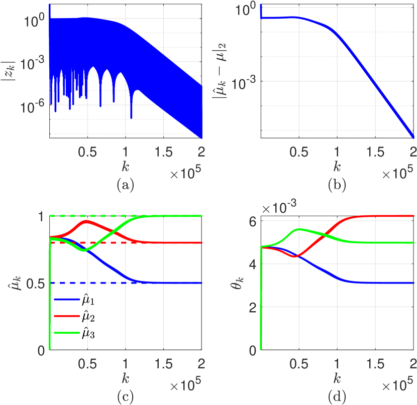
Figure 3: Estimation of three unknown parameters in the nonlinear system (63), (64). (a) shows the output error, (b) shows the parameter error, (c) shows the parameter estimate, and (d) shows the parameter estimator coefficients.

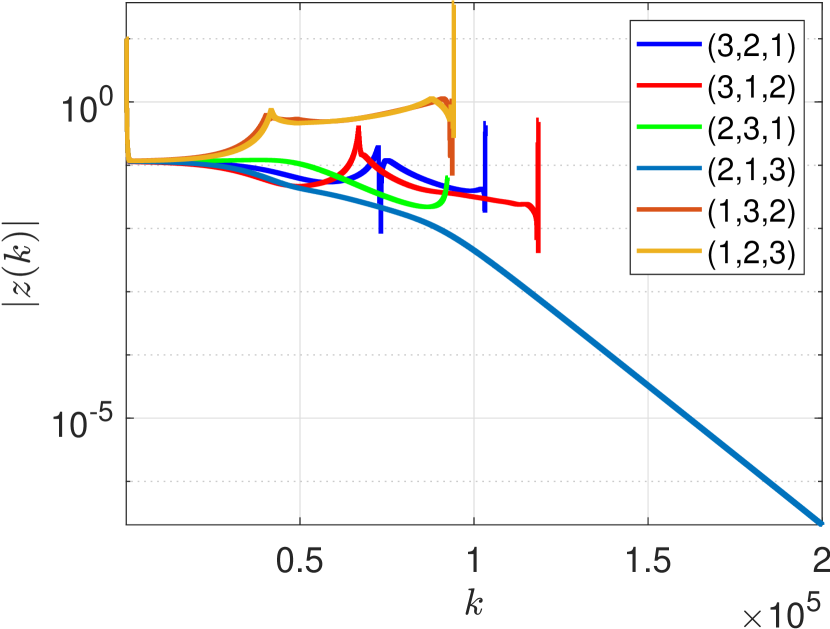
Figure 4: Estimation of three unknown parameters in the nonlinear system (63), (64). Output error for all six permutations. [For clarity, only a subset of the data is plotted.] For five of the six permutations, the parameter error diverges. However, the remaining permutation (2,1,3) yields convergence to the true parameters.

Next, to investigate the relationship between the choice of the filter and the permutation matrix ${\mathcal{O}}_{\rm p}$ that yields convergence, consider the filter

$$G_{{\rm f}}({\textbf{{q}}})=\frac{\sigma_{1}N_{1}}{{\textbf{{q}}}}+\frac{\sigma_{2}N_{2}}{{\textbf{{q}}}}+\frac{\sigma_{3}N_{3}}{{\textbf{{q}}}},$$ (66)

where, for $i=1,2,3,$ $N_{i}\in\{e_{1},e_{2},e_{3}\}$ and $\sigma_{i}\in\{\pm 1\}.$ Note that $e_{i}$ is the $i$th row of the $3\times 3$ identity matrix. Since there are six permutations of the set $\{e_{1},e_{2},e_{3}\},$ there are six choice of the filter coefficients that satisfy Lemma 1. The choices of coefficients $N_{1},N_{2},$ and $N_{3}$ are given in Table 1a. For each choice of the filter coefficients, exactly one permutation matrix yields convergence, which is shown in the fourth column of Table 1a, whereas all other permutations lead to divergence of the output error $z_{k}$. Note that the correct permutation is obtained by checking all permutations in numerical simulations.

Furthermore, for each choice of the filter coefficients, there are eight possible combinations of $\sigma_{1},$ $\sigma_{2},$ and $\sigma_{3},$ which are listed in Table 1b. With the correct permutation matrix choice for each choice of the filter $G_{\rm f}({\textbf{{q}}})$, the coefficients $N_{i}$ are multiplied by $\sigma_{i}$ given in Table 1b. There are thus 48 possible filters.

For each choice of the scalar multipliers $\sigma_{i}$, the pre-estimate $\nu_{k}$ converges to a point in ${\mathcal{S}}_{{\mathcal{O}}_{\rm p}}$ as shown in Figure 5. Note that each point in ${\mathcal{S}}_{{\mathcal{O}}_{\rm p}}$ maps to $\mu$, and the parameter estimate $\hat{\mu}_{k}$ converges to $\mu$ in each case.

This example shows that there exists at least one permutation matrix that yields convergence for every choice of the filter coefficients considered in this example. Furthermore, the element of ${\mathcal{S}}_{{\mathcal{O}}_{\rm p}}$ to which the parameter pre-estimate converges depends on $\sigma_{i}.$ However, since each element of ${\mathcal{S}}_{{\mathcal{O}}_{\rm p}}$ is mapped to the true value of the unknown parameter, the choice of $\sigma_{i}$ is not critical. In fact, all possible combinations of $\sigma_{i}$ yield parameter convergence. $\diamond$

Case	$N_{1}$	$N_{2}$	$N_{3}$	${\rm p}$
1	$[1\ 0\ 0]$	$[0\ 1\ 0]$	$[0\ 0\ 1]$	$(2,1,3)$
2	$[1\ 0\ 0]$	$[0\ 0\ 1]$	$[0\ 1\ 0]$	$(3,1,2)$
3	$[0\ 1\ 0]$	$[1\ 0\ 0]$	$[0\ 0\ 1]$	$(1,2,3)$
4	$[0\ 1\ 0]$	$[0\ 0\ 1]$	$[1\ 0\ 0]$	$(3,2,1)$
5	$[0\ 0\ 1]$	$[0\ 1\ 0]$	$[1\ 0\ 0]$	$(2,3,1)$
6	$[0\ 0\ 1]$	$[1\ 0\ 0]$	$[0\ 1\ 0]$	$(1,3,2)$

(a)

Filter	$\sigma_{1}$	$\sigma_{2}$	$\sigma_{3}$
$G_{{\rm f}1}$	$1$	$1$	$1$
$G_{{\rm f}2}$	$-1$	$1$	$1$
$G_{{\rm f}3}$	$1$	$-1$	$1$
$G_{{\rm f}4}$	$1$	$1$	$-1$
$G_{{\rm f}5}$	$-1$	$-1$	$1$
$G_{{\rm f}6}$	$1$	$-1$	$-1$
$G_{{\rm f}7}$	$-1$	$1$	$-1$
$G_{{\rm f}8}$	$-1$	$-1$	$-1$

(b)

Table 1: Filter coefficients and the permutation used in RCPE to estimate the unknown parameters in the nonlinear system (63), (64).

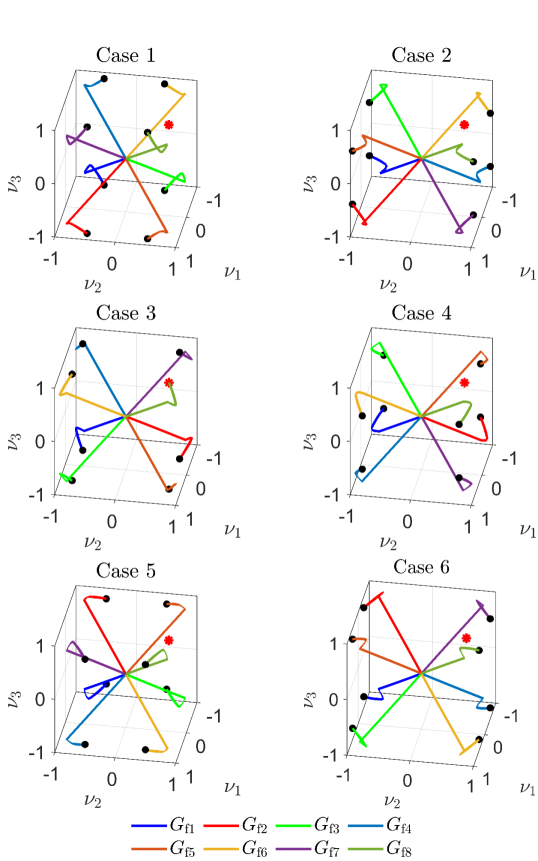
Figure 5: Estimation of three unknown parameters in the nonlinear system (63), (64). Each case shows the parameter pre-estimate $\nu_{k}$ for the choice of $G_{\rm f}$ and ${\mathcal{O}}_{\rm p}$ given in Table 1a and the scalers $\sigma_{i}$ given in Table 1b.

6 Parameter Estimation in the Generalized Burgers Equation

Consider the generalized one-dimensional viscous Burgers equation [33]

$$\frac{\partial u}{\partial t}+\mu_{1}\frac{\partial}{\partial x}\frac{u^{2}}{2}=\frac{\partial}{\partial x}\left(\mu_{2}\frac{\partial u}{\partial x}\right),$$ (67)

where $u(x,t)$ is a function of space and time with domain $[0,1]\times[0,\infty)$, $\mu_{1}>0$ is the convective constant, and $\mu_{2}>0$ is the viscosity. Note that there is no external input to the system (67) and $u$ denotes the solution of this partial differential equation. Let the initial condition be $u(x,0)=0$ for all $x\in[0,1]$, and consider the boundary conditions $u(0,t)=0$ and $u(1,t)=\sin(5t)+0.25\sin(10t)$ for all $t\geq 0.$

The Burgers equation (67) is discretized using a forward Euler approximation for the time derivative, a second-order-accurate upwind method for the convective term, and a second-order-accurate central difference scheme for the viscous term. The spatial domain $[0,1]$ is discretized using $N$ equally spaced grid points; thus $\Delta x\stackrel{{\scriptstyle\triangle}}{{=}}\frac{1}{N-1}$. The time step $\Delta t$ is chosen to satisfy the Courant–Friedrichs–Lewy (CFL) condition, that is,

$$\Delta t<\frac{C_{\rm max}\Delta x}{|{\rm max}(u)|},$$ (68)

where the Courant number $C_{\rm max}$ depends on the discretization scheme [34]. Finally, the discrete variable $u_{j,k}\stackrel{{\scriptstyle\triangle}}{{=}}u((j-1)\Delta x,k\Delta t)$ is defined on the grid points $j\in\{1,\ldots,N\}$ for all time steps $k\geq 0$. Hence, at each grid point, $j\in\{3,\ldots,N-1\}$,

$$u_{j,k+1}=u_{j,k} -\mu_{1}\frac{\Delta t}{2\Delta x}(1.5u_{j,k}^{2}-2u_{j-1,k}^{2}+0.5u_{j-2,k}^{2})+$$

$$\quad\mu_{2}\frac{\Delta t}{\Delta x^{2}}(u_{j+1,k}-2u_{j,k}+u_{j-1,k}).$$ (69)

For all $k\geq 0,$ the discretized boundary conditions are

$$u_{1,k}=u_{2,k}=0,\quad u_{N,k}=\sin(5\Delta tk)+0.25\sin(10\Delta tk),$$ (70)

and, for all $j\in\{3,\ldots,N-1\},$ the initial condition is

$$u_{j}(0)=0.$$ (71)

Finally, for all $k\geq 0,$ let the measurement $y_{k}$ be given by

$$y_{k}\stackrel{{\scriptstyle\triangle}}{{=}}u_{87,k}=u(0.87,k\Delta t).$$ (72)

In this example, $\mu_{1}=1.4,\mu_{2}=0.3$, $C_{\rm max}=0.25$, $N=100$, and $\Delta t=10^{-4}$ s. Figure 6a shows the numerical solution of (69) with the boundary conditions (70) and initial conditions (71), where the solid black line shows the measurement location. Figure 6b shows the measurement $y_{k}.$ The objective is to estimate the unknown parameter $\mu\stackrel{{\scriptstyle\triangle}}{{=}}[\mu_{1}\ \ \mu_{1}]^{\rm T}$ using the scalar measurement $y_{k}$. Thus, $l_{\mu}=2$ and $l_{y}=1.$

In order to start the estimation model, nonzero values of $\hat{\mu}_{1}(0)$ and $\hat{\mu}_{2}(0)$ are needed. A simple way to ensure nonzero values of the estimates is to replace $\mu$ by $\hat{\mu}_{k}=\overline{\mu}+{\mathcal{O}}_{\rm p}|\nu_{k}|$, where $\overline{\mu}=[\overline{\mu}_{1}\ \ \overline{\mu}_{1}]^{\rm T}=[1\ \ 0.01]^{\rm T}$, so that $\hat{\mu}(0)\neq 0$ . In RCPE, let $N_{1}=[1\ 0]$, $N_{2}=[0\ 1]$, $\lambda=0.9999,$ and $R_{\theta}=10^{6}I_{2}$. Let ${\rm p}=(2,1)$ so that ${\mathcal{S}}_{{\mathcal{O}}_{\rm p}}=\{[\pm(\mu_{2}-\overline{\mu}_{2})\ \pm(\mu_{1}-\overline{\mu}_{2})]^{\rm T}\}$. Figure 7 shows the output error, norm of the parameter error, the parameter estimates, and estimator coefficient. Figure 7 also shows the diverging output error for the permutation ${\rm p}=(1,2)$.

This example shows that RCPE can successfully estimate unknown parameters in large-scale computational models without using ensembles and gradients. UKF, on the other hand, would have required an ensemble of 203 models each with 101 state updates resulting in over 20,000 state updates at each step. Furthermore, the sigma points constructed by UKF to propagate the covariance may violate the physical laws or may excite unstable modes in the dynamics, and thus some ensemble members may diverge. In contrast, RCPE updates only the parameter estimate, which can be saturated to constrain the estimate to physically realistic parameter values. $\diamond$

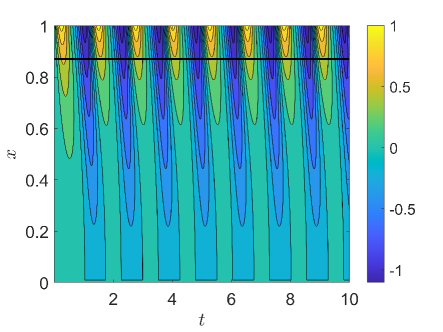
(a)

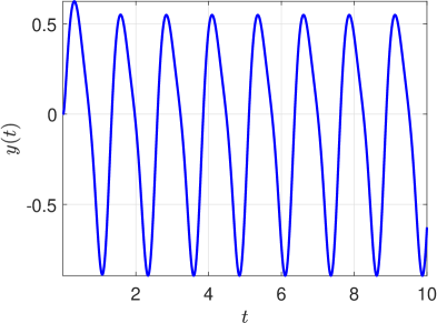
(b)

Figure 6: Simulation of the generalized Burgers equation (67) with the discretization (69). (a) shows the variable $u(x,t)$, and (b) shows the measurement $y(t)$. The magnitude of $u(x,t)$ is shown in the color bar, and the black line denotes the location of the measurement.

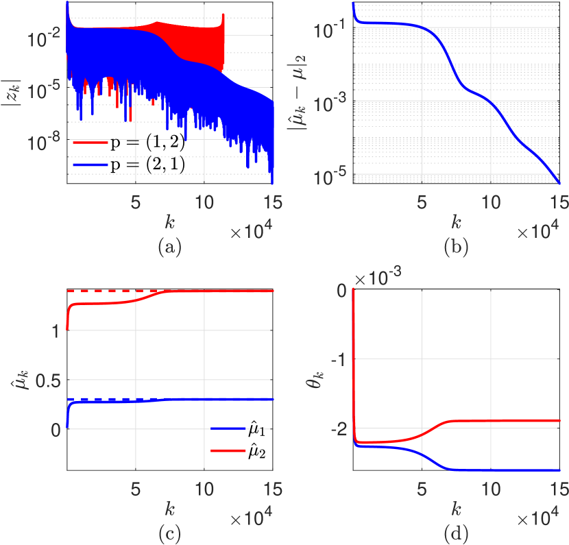
Figure 7: Estimation of two parameters in the generalized Burgers equation (67). (a) shows the output error for both permutation matrices, (b) shows the parameter error, (c) shows the parameter estimates, and (d) shows the parameter estimator coefficients for ${\rm p}=(2,1).$

7 Global Ionosphere-Thermosphere Model

GITM is a computational code that models the thermosphere and the ionosphere of the Earth as well as that of various planets and moons by solving coupled continuity, momentum, and energy equations [1]. By propagating the governing equations, GITM computes neutral, ion, and electron temperatures, neutral-wind and plasma velocities, and mass and number densities of neutrals, ions, and electrons.

GITM uses a uniform grid in latitude with width $\frac{2\pi}{n_{\rm{lat}}}$ rad, where $n_{\rm{lat}}$ is the number of grid points. In longitude and altitude, GITM uses a stretched grid to account for temperature and density variations. GITM is implemented in parallel, where the computational domain (the atmosphere from 100 km to 600 km) is divided into blocks. Ghost cells border the physical blocks to exchange information. GITM can be run either in one-dimensional mode, where horizontal transport is ignored, or in global three-dimensional mode. Furthermore, GITM can be run at either a constant or a variable time step, which is calculated by GITM based on the physical state and the user-defined CFL number in order to maintain numerical stability.

To initialize GITM, neutral and ion densities and temperatures for a chosen time are set using the Mass Spectrometer and Incoherent Scatter radar (MSIS) model [35] and International Reference Ionosphere (IRI) [36]. The model inputs for GITM are $10.7$ cm solar radio flux (F10.7 index), hemispheric power index (HPI), interplanetary magnetic field (IMF), solar wind plasma (SWP), and solar irradiance, all of which are read from a text file containing the time of measurements and the measured values. These signals are available from various terrestrial sensor platforms.

RCPE has previously been used to compensate for the dynamic cooling process [37], estimate the solar irradiance F10.7 [38], and estimate the eddy diffusion coefficient [30] in GITM. In this study, parameters modeling the thermal conductivity coefficient that model the thermal conductity in GITM are estimated.

The temperature at a given altitude depends on the vertical temperature gradient is described by

$$\frac{\delta T}{\delta t}\propto\frac{\delta}{\delta z}\lambda_{\rm c}\frac{\delta T}{\delta z},$$ (73)

where $T$ is absolute temperature, $t$ is time, and $z$ is altitude. The thermal conductivity $\lambda_{\rm c}$ is modeled as

$$\lambda_{\rm c}=\sum_{i\in\{{\rm O,O_{2},N_{2}}\}}\left(\frac{N_{i}}{N_{\rm total}}\right)\kappa_{i}T^{S},$$ (74)

where $\kappa_{i}$ is the thermal-conductivity coefficient of the $i$th species, $N_{i}$ is the number density of the $i$th species, and $S$ is the temperature exponent. The thermal conductivity parameterizes the hydrodynamic transport process that describes the movement of heat through the atmosphere. In GITM, heat is transferred by collisions of the particles in the thermosphere (100 km to 600 km). The three main constituents in the thermosphere are molecular nitrogen $\rm N_{2}$ and oxygen $\rm O_{2}$ and atomic oxygen ${\rm O}$, with the molecular species dominating below about 200 km altitude. Therefore, each of these constituents are included in (74). Furthermore, since the molecular species conduct heat in similar ways, the thermal-conductivity coefficient $\kappa_{{\rm N}_{2}}$ is assumed to be equal to the thermal-conductivity coefficient $\kappa_{{\rm O}_{2}}$ in (74). In this example, the unknown parameters $\kappa_{{\rm O}},\kappa_{{\rm O}_{2}},$ and $S$ in (74) are estimated.

To obtain neutral-density data, the thermosphere is simulated using GITM from 11-21-2002 to 12-05-2002 with the constant thermal-conductivity coefficients $\kappa_{{\rm O}_{2}}=3.6\times 10^{-4}\ {\rm m^{2}/s}$ and $\kappa_{\rm O}=5.6\times 10^{-4}\ {\rm m^{2}/s}$ as well as the temperature exponent $S=6.9\times 10^{-1}$. The neutral density is sampled at intervals of 1 min, and thus the simulated time, which is measured in days, is given by $k/1440,$ where $k\geq 0$ is the number of simulated minutes. At each sample time, the global minimum density $\rho_{\rm min}$, the global maximum density $\rho_{\rm max},$ and the mean density $\rho_{\rm mean}$ at the altitude 300 km are computed. This simulated data, shown in Figure 8, is used by RCPE in the examples below. Only the data after 2 hr (0.083 day) is used in order to avoid the initial transient.

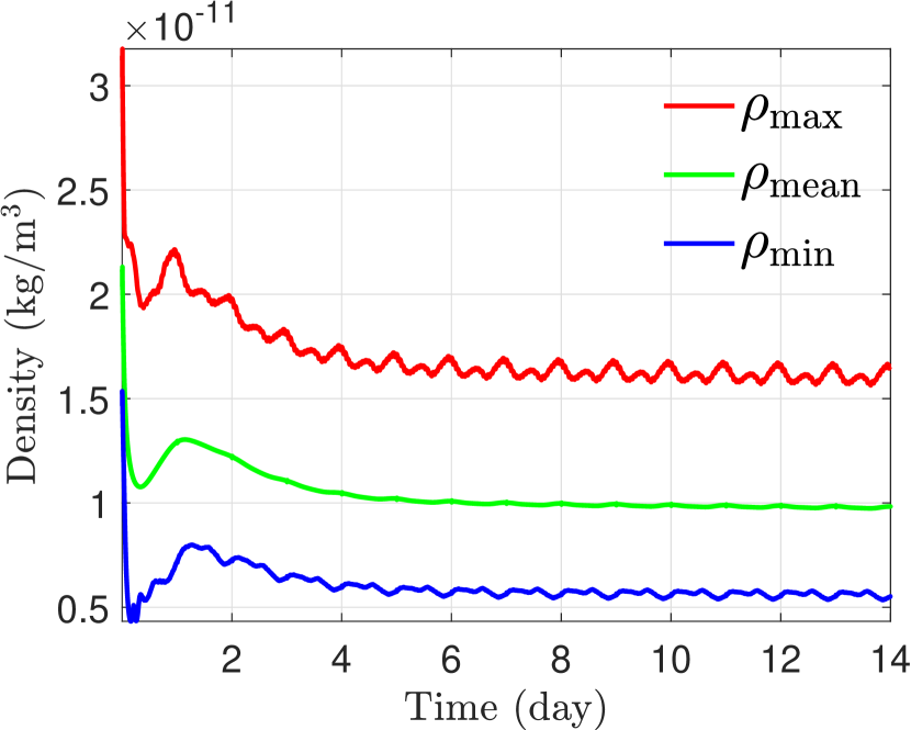
Figure 8: Simulated neutral-density measurements. These measurements are synthesized using the computed neutral density at the altitude 300 km.

In the estimation model, the thermal conductivity coefficients estimates are given by

$$\left[\begin{array}[]{c}\hat{\kappa}_{{\rm O}_{2},k}\\ \hat{\kappa}_{{\rm O},k}\\ \hat{S}_{k}\end{array}\right]=\left[\begin{array}[]{c}\hat{\kappa}_{{\rm O}_{2},0}\\ \hat{\kappa}_{{\rm O},0}\\ \hat{S}_{0}\end{array}\right]+{\mathcal{O}}_{\rm p}|M\nu_{k}|,$$ (75)

where $\hat{\kappa}_{{\rm O}_{2},0}=1.5\times 10^{-4}\,\rm m^{2}/s$ is the initial estimate of $\kappa_{{\rm O}_{2}}=0.5\times 10^{-4}\,\rm m^{2}/s$, $\hat{\kappa}_{{\rm O},0}$ is the initial estimate of $\kappa_{{\rm O}}$, $\hat{S}_{0}=3\times 10^{-1}$ is the initial estimate of $S$, ${\mathcal{O}}_{\rm p}=I_{3}$, $M={\rm diag}(1,1,1000)$, and $\nu_{k}$ is given by (27). Note that the scaling matrix $M$ ensures that all elements of $\nu_{k}$ have similar magnitude. The output of the estimation model is $\hat{y}_{k}=10^{10}[\hat{\rho}_{{\rm min},k}\ \ \hat{\rho}_{{\rm mean},k}\ \ \hat{\rho}_{{\rm max},k}]^{\rm T}$, where the scaling ensures that the error $z_{k}$ and the parameter estimate $\hat{\mu}_{k}$ have similar magnitude. In RCPE, Figure 9 shows the output error, the estimates of $\kappa_{{\rm O}_{2}}$, $\kappa_{{\rm O}}$, and $S$, the norm of the parameter error $\hat{\mu}_{k}-\mu$, and the parameter estimator coefficients $\theta_{k}$. Figure 10 shows the output error for all six choices of ${\rm p}$. Note that the output error diverges for all but one choice of ${\rm p}$.

This application shows that RCPE is an effective technique for removing various sources of model bias using a limited set of observational data. Additionally, the density estimates are also improved as the parameter estimate is improved by RCPE. $\diamond$

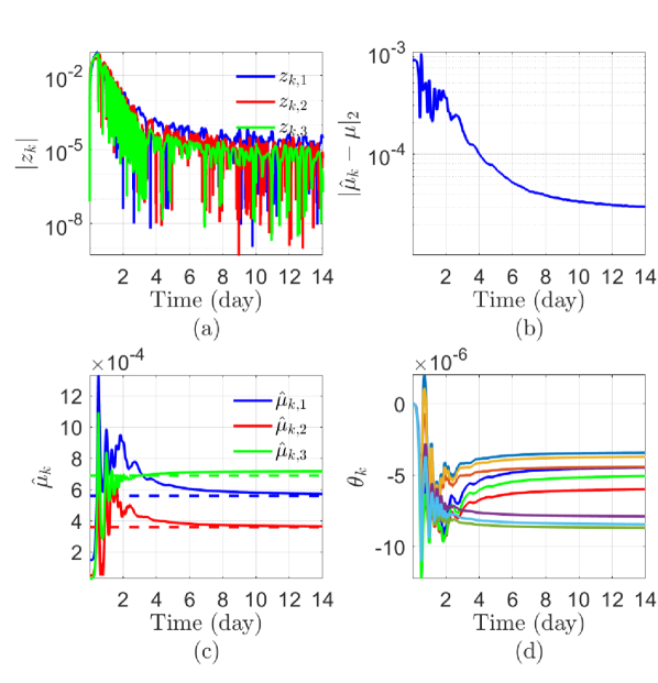
Figure 9: Estimation of $\kappa_{{\rm O}_{2}},\kappa_{{\rm O}},$ and $S$ using measurements of $\rho_{\rm min},\rho_{\rm max}$, and $\rho_{\rm mean}$. (a) shows the output error, (b) shows the parameter error, (c) shows the parameter estimates, and (d) shows the parameter estimator coefficients.

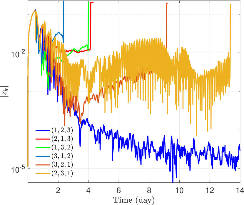
Figure 10: Estimation of $\kappa_{{\rm O}_{2}},$ $\kappa_{{\rm O}},$ and $S$ using measurements of $\rho_{\rm min},$ $\rho_{\rm max}$, and $\rho_{\rm mean}$. The output error is shown for all six permutations of the estimates of $\kappa_{{\rm O}_{2}}$, $\kappa_{{\rm O}}$, and $S$ using $\rho_{\rm min}$, $\rho_{\rm max}$, and $\rho_{\rm mean}$. Note that the output error converges for the permutation (1,2,3), but diverges for the remaining five permutations.

8 Conclusions

Motivated by the need to estimate representational parameters in large-scale models in DDDAS systems, this chapter reviewed the retrospective cost parameter estimation technique. This approach to parameter estimation is both modular and computationally inexpensive since it does not rely on the computation of gradients or the propagation of ensembles. However, in the worst case scenario, the RCPE algorithm may need to be executed $l_{\mu}!$ times in order to determine the parameter permutation that yields convergence of the parameters to the true values.

References

- [1] A J Ridley, Y Deng and G Toth “The global ionosphere–thermosphere model” In J. Atmos. Solar-Terr. Phys. 68, 2006, pp. 839–864 DOI: 10.1016/j.jastp.2006.01.008
- [2] Ror Bellman and Karl Johan Åström “On structural identifiability” In Mathematical biosciences 7.3-4 Elsevier, 1970, pp. 329–339 DOI: 10.1016/0025-5564(70)90132-X
- [3] M. Grewal and K. Glover “Identifiability of linear and nonlinear dynamical systems” In IEEE Trans. Autom. Contr. 21, 1976, pp. 833–837 DOI: 10.1109/TAC.1976.1101375
- [4] S Stanhope, J E Rubin and David Swigon “Identifiability of linear and linear-in-parameters dynamical systems from a single trajectory” In SIAM Journal on Applied Dynamical Systems 13.4 SIAM, 2014, pp. 1792–1815 DOI: 10.1137/130937913
- [5] I M Y Mareels, R R Bitmead, M Gevers, C R Johnson, R L Kosut and M A Poubelle “How exciting can a signal really be?” In Systems & Control Letters 8 North-Holland, 1987, pp. 197–204 DOI: 10.1016/0167-6911(87)90027-2
- [6] Jan C Willems, Paolo Rapisarda, Ivan Markovsky and Bart LM De Moor “A note on persistency of excitation” In Systems & Control Letters 54.4 Elsevier, 2005, pp. 325–329 DOI: 10.1016/j.sysconle.2004.09.003
- [7] S… Islam and D.. Bernstein “Recursive Least Squares for Real-Time Implementation [Lecture Notes]” In IEEE Control Systems Magazine 39.3, 2019, pp. 82–85 DOI: 10.1109/MCS.2019.2900788
- [8] J.-N. Juang “Applied System Identification” Upper Saddle River, NJ: Prentice-Hall, 1993
- [9] L Ljung and T Soderstrom “Theory and Practice of Recursive Identification” The MIT Press, 1983
- [10] L Ljung “System Identification: Theory for the User”, Prentice Hall Information and System Sciences Series Prentice Hall, 1999
- [11] A. Goel, A.. Bruce and D.. Bernstein “Recursive Least Squares With Variable-Direction Forgetting: Compensating for the Loss of Persistency” In IEEE Control Systems Magazine 40.4, 2020, pp. 80–102 DOI: 10.1109/MCS.2020.2990516
- [12] Stephen Boyd and Lieven Vandenberghe “Convex Optimization” Cambridge University Press, 2004 DOI: 10.1017/CBO9780511804441
- [13] O. Kouba and D.. Bernstein “What Is the Adjoint of a Linear System?” In IEEE Control Systems Magazine 40.3, 2020, pp. 62–70 DOI: 10.1109/MCS.2020.2976389
- [14] Tommi S. Jaakkola and Michael I. Jordan “Bayesian parameter estimation via Variational methods” In Statistics and Computing 10 Kluwer Academic Publishers, 2000, pp. 25–37 DOI: 10.1023/A:100893241
- [15] R L Raffard, K Amonlirdviman, J D Axelrod and C J Tomlin “An adjoint-based parameter identification algorithm applied to planar cell polarity signaling” In IEEE Transactions on Automatic Control 53 IEEE, 2008, pp. 109–121 DOI: 10.1109/TAC.2007.911362
- [16] Mette Eknes and Geir Evensen “Parameter estimation solving a weak constraint variational formulation for an Ekman model” In Journal of Geophysical Research: Oceans 102 Wiley Online Library, 1997, pp. 12479–12491 DOI: 10.1029/96JC03454
- [17] Dan Simon “Optimal state estimation: Kalman, H infinity, and nonlinear approaches” John Wiley & Sons, 2006
- [18] L Ljung “Asymptotic behavior of the Extended Kalman filter as a parameter estimator for linear systems” In IEEE Transactions on Automatic Control 24, 1979, pp. 36–50 DOI: 10.1109/TAC.1979.1101943
- [19] Gregory L. Plett “Extended Kalman filtering for battery management systems of LiPB-based HEV battery packs - Part 3. State and parameter estimation” In Journal of Power Sources 134 Elsevier, 2004, pp. 277–292 DOI: 10.1016/j.jpowsour.2004.02.033
- [20] R. Van der Merwe and E A. Wan “The square-root unscented Kalman filter for state and parameter-estimation” In Proceedings of IEEE International Conference on Acoustics, Speech, and Signal Processing 6, 2001, pp. 3461–3464 IEEE DOI: 10.1109/ICASSP.2001.940586
- [21] Eric A. Wan and Rudolph Van Der Merwe “The unscented Kalman filter for nonlinear estimation” In Adaptive Systems for Signal Processing, Communications, and Control Symposium IEEE, 2000, pp. 153–158 DOI: 10.1109/ASSPCC.2000.882463
- [22] G. Evensen “The ensemble Kalman filter for combined state and parameter estimation” In IEEE Control Systems Magazine 29, 2009, pp. 83–104 DOI: 10.1109/MCS.2009.932223
- [23] H Moradkhani, S Sorooshian, H V Gupta and P R Houser “Dual state and parameter estimation of hydrological models using ensemble Kalman filter” In Advances in Water Resources 28, 2005, pp. 135–147 DOI: 10.1016/j.advwatres.2004.09.002
- [24] Reza Madankan, Puneet Singla, Tarunraj Singh and Peter D. Scott “Polynomial-chaos-based Bayesian approach for state and parameter estimations” In Journal of Guidance, Control, and Dynamics 36, 2013, pp. 1058–1074 DOI: 10.2514/1.58377
- [25] Joe D Hoffman and Steven Frankel “Numerical methods for engineers and scientists” CRC press, 2018
- [26] Yousaf Rahman, Antai Xie and Dennis S. Bernstein “Retrospective Cost Adaptive Control: Pole Placement, Frequency Response, and Connections with LQG Control” In IEEE Control System Magazine 37, 2017, pp. 28–69 DOI: 10.1109/MCS.2017.2718825
- [27] Ankit Goel and Dennis S Bernstein “Gradient-, Ensemble-, and Adjoint-Free Data-Driven Parameter Estimation” In Journal of Guidance, Control, and Dynamics 42.8 American Institute of AeronauticsAstronautics, 2019, pp. 1743–1754 DOI: 10.2514/1.G004158
- [28] Ankit Goel, Brandon Ponder, Aaron Ridley and Dennis S Bernstein “Estimation of Thermal-Conductivity Coefficients in the Global Ionosphere–Thermosphere Model” In Journal of Aerospace Information Systems 17.9 American Institute of AeronauticsAstronautics, 2020, pp. 546–553 DOI: 10.2514/1.I010819
- [29] A. Goel and D.. Bernstein “Data-Driven Parameter Estimation for Models with Nonlinear Parameter Dependence” In Proc. Conf. Dec. Contr., 2018, pp. 1470–1475 DOI: 10.1109/CDC.2018.8619566
- [30] Ankit Goel, Aaron Ridley and Dennis S. Bernstein “Estimation of the Eddy Diffusion Coefficient Using Total Electron Content Data” In Proc. Amer. Contr. Conf., 2018, pp. 3298–3303 DOI: 10.23919/ACC.2018.8431184
- [31] A. Goel, K. Duraisamy and D.. Bernstein “Parameter Estimation in the Burgers Equation Using Retrospective-Cost Model Refinement” In Proc. Amer. Contr. Conf., 2016, pp. 6983–6988 DOI: 10.1109/ACC.2016.7526773
- [32] M… Kulenović and G.. Ladas “Dynamics of second order rational difference equations: With open problems and conjectures” Chapman & Hall/CRC, 2002, pp. 218
- [33] David T Blackstock “Generalized Burgers equation for plane waves” In The Journal of the Acoustical Society of America 77.6 Acoustical Society of America, 1985, pp. 2050–2053 DOI: 10.1121/1.391778
- [34] Richard Courant, Kurt Friedrichs and Hans Lewy “On the partial difference equations of mathematical physics” In IBM Journal of Research and Development 11 IBM, 1967, pp. 215–234 DOI: 10.1147/rd.112.0215
- [35] Alan E Hedin “Extension of the MSIS thermosphere model into the middle and lower atmosphere” In J. Geophys. Res.: Space Phys. 96.A2, 1991, pp. 1159–1172 DOI: 10.1029/90JA02125
- [36] Dieter Bilitza “International reference ionosphere 2000” In Radio Sci. 36.2 Wiley Online Library, 2001, pp. 261–275 DOI: 10.1029/2000RS002432
- [37] Anthony M. D’Amato, Aaron J. Ridley and Dennis S. Bernstein “Retrospective-cost-based adaptive model refinement for the ionosphere and thermosphere” In Statistical Analysis and Data Mining 4 Wiley-Blackwell, 2011, pp. 446–458 DOI: 10.1002/sam.10127
- [38] A.. Ali, A. Goel, A.. Ridley and D.. Bernstein “Retrospective-Cost-Based Adaptive Input and State Estimation for the Ionosphere–Thermosphere” In J. Aero. Inf. Sys. 12.12 American Institute of AeronauticsAstronautics, 2015, pp. 767–783 DOI: 10.2514/1.I010286