A tutorial introduction to quantum stochastic master equations based on the qubit/photon system
Abstract
From the key composite quantum system made of a two-level system (qubit) and a harmonic oscillator (photon) with resonant or dispersive interactions, one derives the corresponding quantum Stochastic Master Equations (SME) when either the qubits or the photons are measured. Starting with an elementary discrete-time formulation based on explicit formulae for the interaction propagators, one shows how to include measurement imperfections and decoherence. This qubit/photon quantum system illustrates the Kraus-map structure of general discrete-time SME governing the dynamics of an open quantum system subject to measurement back-action and decoherence induced by the environment. Then, on the qubit/photon system, one explains the passage to a continuous-time mathematical model where the measurement signal is either a continuous real-value signal (typically homodyne or heterodyne signal) or a discontinuous and integer-value signal obtained from a counter. During this derivation, the Kraus map formulation is preserved in an infinitesimal way. Such a derivation provides also an equivalent Kraus-map formulation to the continuous-time SME usually expressed as stochastic differential equations driven either by Wiener or Poisson processes. From such Kraus-map formulation, simple linear numerical integration schemes are derived that preserve the positivity and the trace of the density operator, i.e. of the quantum state.
Keywords:
Open quantum systems, decoherence, quantum stochastic master equation, Lindblad master equation, Kraus-map, quantum channel, quantum filtering, Wiener process, Poisson process, qubit/photon composite system. Positivity and trace preserving numerical scheme.
1 Intoduction
An increasing number of experiments controlling quantum states are conducted with various physical supports such as spins, atoms, trapped ions, photons, superconducting circuits, electro-mechanical circuits, optomechanical cavities (see, e.g., [25, 19, 7, 20, 13]). As illustrated on Fig. 1, the quantum dynamics of these experiments can be precisely described by well structured stochastic differential equations, called Stochastic Master Equations (SME). They govern the relationships between the input corresponding to the classical parameters manipulated by the experimentalists and the classical output corresponding to the observed measurements. These SME are expressed with operators for which non-commutative calculus and commutation relationships play a fundamental role. These SME are the quantum analogue of the classical Kalman state-space descriptions, and , with noise [29].
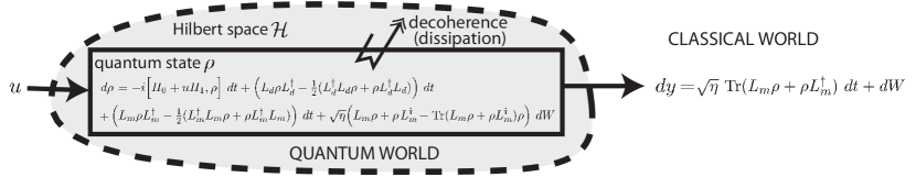
For Fig. 1, with classical input and classical output , this SME reads (diffusive case with Itō formulation [8], stands for Hermitian conjugate of operator ):
| (1) |
where the same Wiener process is shared by the state dynamics and the output map
| (2) |
The state is a density operator (a self-adjoint, non-negative and trace-one operator) on a Hilbert space . Its dynamics (1) are parameterized here via two self-adjoint operators (Hamiltonians) and ( stands for the commutator) and two Lindblad operators, describing a decoherence channel and a measurement channel of efficiency . When , follows a deterministic linear master equation, called Lindblad master equation with two decoherence channels described by and ,
| (3) |
and the measurement boils down to a Wiener process without any relations with and and thus can be discarded. Notice that (3) corresponds also to the ensemble average dynamics of the SME (1). Notice also that the initial value problems (Cauchy problems) attached to (1) or to (3) are non trivial mathematical problems when the dimension of the underlying Hilbert space is infinite and the Hamiltonian or Lindblad operators are unbounded (see e.g [2, 45]).
These SME rely on the well developed theory of open quantum systems combining irreversibility due to decoherence (quantum dissipation) [18, 14] and stochasticity due to measurement back-action [49, 16, 17, 27, 26]. More general SME than the one depicted on Fig. 1, with several Lindblad operators and/or driven by Poisson processes (counting measurement), admit similar structures [39]. Even if the initial system is known to be non Markovian, it is always possible in general to adjunct a dynamical model of the environment and to recover a Markovian model with an SME structure but of larger dimension [14, part IV]. For composite systems made of several interacting quantum sub-systems such SME models are also derived from a quantum network theory [24, 23] gathering in a concise way, quantum stochastic calculus [35], Heisenberg description of input/output theory [50, 22] and quantum filtering [12].
The goal of this paper is to provide an introduction to the structure of these quantum SME illustrated via a composite system made of two key quantum sub-systems (qubits and photons, see A) and based on three fundamental quantum rules (unitary evolution derived from Schrödinger equation, measurement back-action with the collapse of the wave-packet, composite systems relying on tensor products, see B).
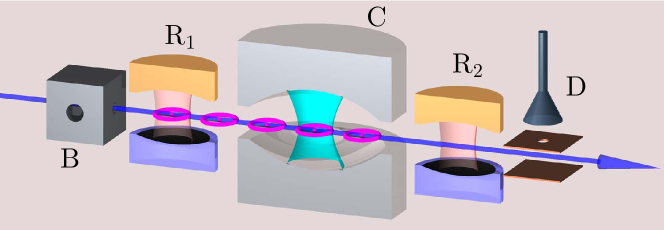
Section 2 is devoted to discrete-time formulation of SME. One starts with the Markov chain modelling the LKB111LKB for Laboratoire Kastler Brossel. photon box of Fig. 2 [25] where photons are measured by probe atoms described by two-level systems, i.e. qubits. Two kinds of interactions between the photons and the atoms are considered (see A for operator notations) :
-
•
dispersive interaction leading to Quantum Non Demolition (QND) measurement of photons; the qubit/photon interaction is dispersive where (with a constant parameter) yields , the Schrödinger propagator during the time , given by the explicit formula:
(4) where .
-
•
resonant interaction stabilizing then the photons in vacuum state; the qubit/photon interaction is here resonant where (with a constant parameter) yields , the Schrödinger propagator during the time , given by the explicit formula:
(5) where .
One explains on this key system how to take into account measurement errors and why the density operator as quantum state is then crucial. One concludes section 2 with the general structure of discrete-time SME governing the stochastic dynamics of open quantum systems subject to unperfect measurement and decoherence.
Section 3 is devoted to continuous-time SME. One considers here the reverse situation where the qubit is measured by probe photons. Dispersive interaction, measurement of one quadrature of the photons (an observable with a continuous spectrum) and scaling as yields a continuous-time SME driven by a Wiener process of form (1) with , and . One shows how measurement errors tend to decrease towards . Then the general structure of diffusive SME is presented with an equivalent Kraus-map formulation yielding alinear time-integration numerical scheme preserving the positivity and the trace. Resonant interaction, measurement of the photon-number operator and scaling as yield a continuous-time SME driven by a Poisson process associated to the measurement counter. One shows how to include measurement imperfections and gives the structure of continuous-time SME driven by Poisson processes. Last subsection of section 3 provides a very general structure of continuous-time SME driven by Wiener and Poisson processes governing the stochastic dynamics of open quantum systems subject to diffusive/counting unperfect measurements and decoherence.
The conclusion section 4 provides some comments and references related to feedback, parameter estimation and filtering issues. These comments and references are far from being exhaustive.
2 Discrete-time formulation
2.1 Photons measured by qubits (dispersive interaction)
The wave function of the photon is denoted here by . From the scheme of Fig. 2, the qubit produced by the in state is subject in to a rotation of in the plane , then interacts during dispersively with the photons in , is subject to the reverse rotation of in and finally is measured in according to . The Schrödinger evolution of the qubit/photon wave function between and just before is given by the following unitary evolution :
Applied to the value of when the qubit leaves , one gets222Tensor sign and tensor product with identity operator are not explicitly recalled in the formula as it is usually done when there is no ambiguity: and read then and ; similarly just becomes .
Measuring in , the observable yields the collapse of into a separable state or , eigen-vectors of with eigenvalues or , respectively. Numbering the qubit by the integer and removing the qubit state, one gets the following Markov process induced by the passage of qubit number :
where is the classical signal produced by the quantum measurement of qubit . The density operator formulation of this Markov process reads ( ):
with measurement Kraus operators and . Notice that .
When is irrational, each realization of this Markov process, starting from satisfying for large enough, converges almost surely towards a Fock state for some . More precisely, the probability that a realisation converges towards is given by the initial population (see, e.g.,[40, 11, 4]). This almost sure convergence can be seen from the following Lyapunov function (super-martingale)
that converges in average towards since its expectation value from step to step satisfies :
2.2 Photons measured by qubits (resonant interaction)
The photon wave function is still denoted by . The qubit coming from box of Fig. 2 is in . The Ramsey zones and are inactive. The resonant interaction during the passage of the qubit in yields the propagator (5). Thus, the wave function of the composite qubit/photon system, just before the qubit measurement in , is as follows:
Therefore, the resulting Markov process associated to the measurement of the observable with classical signal is as follows:
The corresponding density operator formulation is then
with measurement Kraus operators and . Notice that, once again, .
When is irrational for all positive integer , this Markov process converges almost surely towards vacuum state when for large enough. This results from the following the Lyapunov function (super-martingale)
since
2.3 Measurement errors
In presence of measurement imperfections and errors, one has to update the quantum according to Bayes rule by taking as quantum state, the expectation value of given by
knowing and the information provides by the imperfect measurement outcome. Assume firstly, that the detector is broken. Then, we get the following linear, trace-preserving and completely positive map
called in quantum information a quantum channel (see [34]).
When the qubit detector , producing the classical measurement signal , has symmetric errors characterized by the single error rate , the probability of detector outcome (resp. ) knowing that the perfect outcome is (resp. ), Bayes law gives directly
| (6) |
Notice that a broken detector corresponds to and one recovers the above quantum channel.
2.4 Stochastic Master Equation (SME) in discrete-time
In fact, the general structure of discrete-time SME can always be constructed from the knowledge of a quantum channel (trace preserving completely positive map) having the following Kraus decomposition (which is not unique)
and a left stochastic matrix where corresponds to the different imperfect measurement outcomes. Set . The SME associated to and reads
Notice that since is left stochastic. Here the Hilbert space is arbitrary and can be of infinite dimension, the Kraus operator are bounded operator on and is a density operator on (Hermitian, trace-class with trace one, non-negative).
3 Continuous-time formulation
Contrarily to section 2, photons measure here a qubit.
3.1 Qubits measured by photons: dispersive interaction and discrete-time
The qubit wave function is denoted by . The photons, before interacting with the qubit, are in the coherent state with real and strictly positive. The interaction is dispersive according to (4). After the interaction and just before the measurement performed on the photons, the composite qubit/photon wave function reads:
since for any coherent state of complex amplitude , is also a coherent state of complex amplitude ().
Assume that the perfect measurement outcome belongs to and corresponds to the phase-plane observable having the entire real line as spectrum. Its spectral decomposition reads formally where is the wave function associated to the eigen-value . is not a usual wave function, i.e., in , but one has formally (see, e.g., [9]). Since
we have
Thus
where with probability .
The density operator formulation reads then
and measurement Kraus operators
Notice that
| (7) |
and .
For , one has almost sure convergence towards or deduced from the following Lyapunov function
and
Assume that the detection of is not perfect. The probability density of knowing that the perfect detection is is also a Gaussian given by for some error parameter . Then the above Markov process becomes
where
Standard computations show that
3.2 Dispersive interaction and continuous-time diffusive limit
Consider the above Markov process with perfect detection . From (7), one gets
When , we have up-to third order terms versus ,
Replacing by its expectation value independent of one gets, up to third order terms versus and :
Set and . Since by construction
one has and up to order versus . Thus for very small, we recover the following diffusive SME
with replacing and according to Ito rules.
With measurement errors parameterized by , the partial Kraus map
yields
From
and
one gets
Up to third order terms versus , one has then
Replacing by its average independent of one gets
Set and . Since by construction
one has and . Thus for very small, we recover the following SME with detection efficiency
with corresponding to and a Wiener process satisfying Ito rules .
Convergence towards either or is based on the following Lyapunov fonction . According to Ito rules, one has
where , and . Since , converges exponentially to since governed by the linear differential equation
For more general and precise results on diffusive SME corresponding to QND measurements and measurement-based feedback issues see [10, 32, 15].
3.3 Diffusive SME
As studied in [8], the general form of diffusive SME admits the following Ito formulation:
with efficiencies and being independent Wiener processes. Here the Hilbert space is arbitrary, is Hermitian and are arbitrary operators of not necessarily Hermitian. Each label such that corresponds here to a decoherence channel that can be seen as an unread measurement performed by a sub-system belonging to the environment, see [25, chapter 4].
With Ito rules, this SME admits also the following equivalent formulation:
with
Moreover follows the following probability density knowing :
that remains a linear function of , as imposed by the quantum measurement law.
In finite dimension , this formulation implies directly that any diffusive SME admits a unique solution remaining for all in .
3.4 Kraus maps and numerical schemes for diffusive SME
From the above formulation, one can construct a linear, positivity and trace preserving numerical integration scheme for such diffusive SME (see [28, appendix B]):
With
set
Sampling of according to the following probability law:
where
The update is then given by the following exact Kraus-map formulation:
Notice that the operators and are bounded operators even if and are unbounded.
One can also use the following splitting scheme when the unitary operator is numerically available and where in the above calculations is reduced to :
3.5 Qubits measured by photons (resonant interaction)
The qubit wave function is denoted by . The photons, before interacting with the qubit, are in the vacuum state . The interaction is resonant according to (5). After the interaction and just before the measurement performed on the photons, the composite qubit/photon wave function reads:
The Markov process with measurement observable and outcome reads (density operator formulation)
with measurement Kraus operators and . Notice that .
Almost convergence analysis when towards can be seen via the Lyapunov function (super martingale)
since
3.6 Towards jump SME
Since in the above Markov process and , one gets with and being denoted by , an SME driven by Poisson process of expectation value knowing :
At each time-step, one has the following choice:
-
•
with probabilty , and
with .
-
•
with probability , and
with .
To take into account shot noise of rate and detection efficiency , consider the following left stochastic matrix
where is the probability to detect , knowing that the true outcome is (fault detection associated to shot noise) and where is the probability to detect knowing that the true outcome is (detection efficiency). Then the above stochastic master equation becomes
At each time-step, one has the following recipe
-
•
and
with probability
and where and .
-
•
and
with probability
3.7 Jump SME in continuous-time
The above computations with very small emphasize the following general structure of a Jump SME in continuous time. With the counting process having increment expectation value knowing given by and detection imperfections modeled by (shot-noise rate) and (detection efficiency), the quantum state is usually mixed and obeys to
Here and are operators on an underlying Hilbert space , being Hermitian. At each time-step between and , one has
-
•
with probability
where .
- •
3.8 General mixed diffusive/jump SME
One can combine in a single SME Wiener and Poisson noises induced by diffusive and counting measurements. The quantum state , usually mixed, obeys to
With and with probability . The Kraus-map equivalent formulation reads:
-
•
for of probability
with .
-
•
for of probability :
More generally, one can consider several independent Wiener and Poisson processes. The corresponding SME reads then
where , with are parameters modelling measurements imperfections.
The equivalent Kraus-map formulation is the following
-
•
When (probability ) we have
with and where .
-
•
If, for some , (probability ) we have a similar transition rule
with
4 Conclusion
These SME driven by diffusive measurements or counting measurements are now the object of numerous control-theoretical and mathematical investigations that can be divided into two main issues. The first issues are related to feedback stabilization of a target quantum state (quantum state preparation) or of quantum subspace as in quantum error correction. One can distinguish several kinds of quantum feedback:
-
•
Markovian feedback [49] which is in fact a static output feedback usually used in discrete-time quantum error correction. Its main interest relies on the closed-loop ensemble average dynamics which is a linear quantum channel for which several stability properties are available (see, e.g.,[34, 36, 43]).
- •
-
•
Coherent feedback where the controller is a quantum dissipative system [24]. It has its origin in optical pumping and coherent population trapping [30, 6]. Such feedback structures are now the object of active researches in the context of autonomous quantum error correction (see, e.g., [48, 41, 31, 33, 37]).
The second issues are related to filtering and estimation. They are closely related to quantum-state or quantum-process tomography:
-
•
Quantum filtering that can be seen as the quantum analogue of state asymptotic observers. It has its origin in the seminal work of [12]. It can be shown that quantum filtering is always a stable process in average (see [38, 3]). Characterization of asymptotic almost-sure convergence is an open-problem with recent progresses (see, e.g., [47, 5]).
- •
Acknowledgment
The author thanks Claude Le Bris, Philippe Campagne-Ibarcq, Zaki Leghtas, Mazyar Mirrahimi, Alain Sarlette and Antoine Tilloy for many interesting discussions on SME modeling and numerics for open quantum systems.
This project has received funding from the European Research Council (ERC) under the European Union’s Horizon 2020 research and innovation programme (grant agreement No. [884762]).
References
- [1] C. Ahn, A. C. Doherty, and A. J. Landahl. Continuous quantum error correction via quantum feedback control. Phys. Rev. A, 65:042301, March 2002.
- [2] R. Alicki and K. Lendi. Quantum Dynamical Semigroups and Applications. Lecture Notes in Physics. Springer, second edition, 2007.
- [3] H. Amini, C. Pellegrini, and P. Rouchon. Stability of continuous-time quantum filters with measurement imperfections. Russian Journal of Mathematical Physics, 21(3):297–315–, 2014.
- [4] H. Amini, R.A. Somaraju, I. Dotsenko, C. Sayrin, M. Mirrahimi, and P. Rouchon. Feedback stabilization of discrete-time quantum systems subject to non-demolition measurements with imperfections and delays. Automatica, 49(9):2683–2692, September 2013.
- [5] Nina H Amini, Maël Bompais, and Clément Pellegrini. On asymptotic stability of quantum trajectories and their cesaro mean. Journal of Physics A: Mathematical and Theoretical, 54(38):385304, sep 2021.
- [6] E. Arimondo. Coherent population trapping in laser spectroscopy. Progr. Optics, 35:257, 1996.
- [7] M. Aspelmeyer, T.J. Kippenberg, and F. Marquardt. Cavity optomechanics. Rev. Mod. Phys., 86(4):1391–1452, December 2014.
- [8] A. Barchielli and M. Gregoratti. Quantum Trajectories and Measurements in Continuous Time: the Diffusive Case. Springer Verlag, 2009.
- [9] S. M. Barnett and P. M. Radmore. Methods in Theoretical Quantum Optics. Oxford University Press, 2003.
- [10] M; Bauer, T. Benoist, and D. Bernard:. Repeated quantum non-demolition measurements: Convergence and continuous time limit. Ann. Henri Poincare, 14:639–679, 2013.
- [11] Michel Bauer and Denis Bernard. Convergence of repeated quantum nondemolition measurements and wave-function collapse. Phys. Rev. A, 84:044103, Oct 2011.
- [12] V.P. Belavkin. Quantum stochastic calculus and quantum nonlinear filtering. Journal of Multivariate Analysis, 42(2):171–201, 1992.
- [13] W.P. Bowen and G.J. Milburn. Quantum Optomechanics. CRC Press, 2016.
- [14] H.-P. Breuer and F. Petruccione. The Theory of Open Quantum Systems. Clarendon-Press, Oxford, 2006.
- [15] G. Cardona, A. Sarlette, and P. Rouchon. Exponential stabilization of quantum systems under continuous non-demolition measurements. Automatica, 112:108719, 2020.
- [16] H. Carmichael. An Open Systems Approach to Quantum Optics. Springer-Verlag, 1993.
- [17] J. Dalibard, Y. Castin, and K. Mølmer. Wave-function approach to dissipative processes in quantum optics. Phys. Rev. Lett., 68(5):580–583, February 1992.
- [18] E.B. Davies. Quantum Theory of Open Systems. Academic Press, 1976.
- [19] M. Devoret, B. Huard, R. Schoelkopf, and L.F. Cugliandolo, editors. Quantum Machines: Measurement Control of Engineered Quantum Systems, volume 96 of Lecture Notes of the Les Houches Summer School, July 2011. Oxford University Press, 2014.
- [20] C. Gardiner and P. Zoller. The Quantum World of Ultra-Cold Atoms and Light Book II: The Physics of Quantum- Optical Devices (1st ed. ). Imperial College Press, London., 2015.
- [21] C. W. Gardiner, A. S. Parkins, and P. Zoller. Wave-function quantum stochastic differential equations and quantum-jump simulation methods. Phys. Rev. A, 46(7):4363–4381, October 1992.
- [22] C.W. Gardiner and P. Zoller. Quantum noise. Springer, third edition, 2010.
- [23] J. Gough and M.R. James. Quantum feedback networks: Hamiltonian formulation. Communications in Mathematical Physics, 287(3):1109–1132–, 2009.
- [24] J. Gough and M.R. James. The series product and its application to quantum feedforward and feedback networks. Automatic Control, IEEE Transactions on, 54(11):2530–2544, 2009.
- [25] S. Haroche and J.M. Raimond. Exploring the Quantum: Atoms, Cavities and Photons. Oxford University Press, 2006.
- [26] K. Jacobs. Quantum measurement theory and its applications. Cambridge University Press, 2014.
- [27] Kurt Jacobs and Daniel A. Steck. A straightforward introduction to continuous quantum measurement. Contemporary Physics, 47(5):279–303, 2006.
- [28] Andrew N. Jordan, Areeya Chantasri, Pierre Rouchon, and Benjamin Huard. Anatomy of fluorescence: quantum trajectory statistics from continuously measuring spontaneous emission. Quantum Studies: Mathematics and Foundations, 3(3):237–263, 2016.
- [29] T. Kailath. Linear Systems. Prentice-Hall, Englewood Cliffs, NJ, 1980.
- [30] A. Kastler. Optical methods for studying Hertzian resonances. Science, 158(3798):214–221, October 1967.
- [31] Z. Leghtas, G. Kirchmair, B. Vlastakis, R.J. Schoelkopf, M.H. Devoret, and M. Mirrahimi. Hardware-efficient autonomous quantum memory protection. Phys. Rev. Lett., 111(12):120501–, September 2013.
- [32] Weichao Liang, Nina H. Amini, and Paolo Mason. On exponential stabilization of n-level quantum angular momentum systems. SIAM Journal on Control and Optimization, 57(6):3939–3960, 2019.
- [33] M. Mirrahimi et al. Dynamically protected cat-qubits: a new paradigm for universal quantum computation. New Journal of Physics, 16:045014, 2014.
- [34] M.A. Nielsen and I.L. Chuang. Quantum Computation and Quantum Information. Cambridge University Press, 2000.
- [35] K.R. Parthasarathy. An Introduction to Quantum Stochastic Calculus. Birkhäuser, 1992.
- [36] D. Petz. Monotone metrics on matrix spaces. Linear Algebra and its Applications, 244:81–96, 1996.
- [37] R. Lescanne et al. Exponential suppression of bit-flips in a qubit encoded in an oscillator. Nat. Phys., 16:509–513, 2020.
- [38] P. Rouchon. Fidelity is a sub-martingale for discrete-time quantum filters. IEEE Transactions on Automatic Control, 56(11):2743–2747, 2011.
- [39] P. Rouchon. Models and Feedback Stabilization of Open Quantum Systems. In Proceedings of International Congress of Mathematicians, volume IV, pages 921–946, 2014. see also: http://arxiv.org/abs/1407.7810.
- [40] S. Haroche, M. Brune, and J.M. Raimond. Measuring photon numbers in a cavity by atomic interferometry: optimizing the convergence procedure. J. Phys. II France, 2(4):659–670, 1992.
- [41] S. Sarlette, M. Brune, J.M. Raimond, and P. Rouchon. Stabilization of nonclassical states of the radiation field in a cavity by reservoir engineering. Phys. Rev. Lett., 107:010402, 2011.
- [42] C. Sayrin, I. Dotsenko, X. Zhou, B. Peaudecerf, Th. Rybarczyk, S. Gleyzes, P. Rouchon, M. Mirrahimi, H. Amini, M. Brune, J.M. Raimond, and S. Haroche. Real-time quantum feedback prepares and stabilizes photon number states. Nature, 477:73–77, 2011.
- [43] R. Sepulchre, A. Sarlette, and P. Rouchon. Consensus in non-commutative spaces. In Decision and Control (CDC), 2010 49th IEEE Conference on, pages 6596–6601, 2010.
- [44] P. Six, Ph. Campagne-Ibarcq, I. Dotsenko, A. Sarlette, B. Huard, and P. Rouchon. Quantum state tomography with noninstantaneous measurements, imperfections, and decoherence. Phys. Rev. A, 93:012109, Jan 2016.
- [45] V.E. Tarasov. Quantum Mechanics of Non-Hamiltonian and Dissipative Systems. Elsevier, 2008.
- [46] Antoine Tilloy. Exact signal correlators in continuous quantum measurements. Phys. Rev. A, 98:010104, Jul 2018.
- [47] R. van Handel. The stability of quantum Markov filters. Infin. Dimens. Anal. Quantum Probab. Relat. Top., 12:153–172, 2009.
- [48] F. Verstraete, M.M. Wolf, and I.J. Cirac. Quantum computation and quantum-state engineering driven by dissipation. Nat Phys, 5(9):633–636, September 2009.
- [49] H.M. Wiseman and G.J. Milburn. Quantum Measurement and Control. Cambridge University Press, 2009.
- [50] B. Yurke and J.S. Denker. Quantum network theory. Phys. Rev. A, 29(3):1419–1437, March 1984.
Appendix A Notations used for qubits and photons
-
1.
The qubit with a two-dimensional Hilbert space:
-
•
Hilbert space: with ortho-normal basis and (Dirac notations).
-
•
Quantum state space:
-
•
Pauli operators and commutations:
,
;
;
;
, , , -
•
Hamiltonian: .
-
•
Bloch sphere representation:
-
•
-
2.
The photons of the quantum harmonic oscillator with an infinite dimensional Hilbert:
-
•
Hilbert space: with the infinite dimensional orthonormal basis .
-
•
Quantum state space: corresponding to trace-class Hermitian operators on with unit trace.
-
•
Operators and commutations:
Annihilation and creation operator: , ;
Number operator: , ;
, for any function ;
Coherent displacement unitary operator .
Position and momentum operators :
. -
•
Hamiltonian: .
(associated classical dynamics: ). -
•
Quasi-classical pure state coherent state ; ; , .
-
•
Appendix B Three quantum rules
This appendix is borrowed from [39]
-
1.
The state of a quantum system is described either by the wave function a vector of length one belonging to some separable Hilbert space of finite or infinite dimension, or, more generally, by the density operator that is a non-negative Hermitian operator on with trace one. When the system can be described by a wave function (pure state), the density operator coincides with the orthogonal projector on the line spanned by and with usual Dirac notations. In general the rank of exceeds one, the state is then mixed and cannot be described by a wave function. When the system is closed, the time evolution of is governed by the Schrödinger equation (here )
(8) where is the system Hamiltonian, an Hermitian operator on that could possibly depend on time via some time-varying parameters (classical control inputs). When the system is closed, the evolution of is governed by the Liouville/von-Neumann equation
(9) -
2.
Dissipation and irreversibility has its origin in the ”collapse of the wave packet” induced by the measurement. A measurement on the quantum system of state or is associated to an observable , an Hermitian operator on , with spectral decomposition : is the orthogonal projector on the eigen-space associated to the eigen-value ( for ). The measurement process attached to is assumed to be instantaneous and obeys to the following rules:
-
•
the measurement outcome is obtained with probability or , depending on the state or just before the measurement;
-
•
just after the measurement process, the quantum state is changed to or according to the mappings
where is the observed measurement outcome. These mappings describe the measurement back-action and have no classical counterpart.
-
•
-
3.
Most systems are composite systems built with several sub-systems. The quantum states of such composite systems live in the tensor product of the Hilbert spaces of each sub-system. This is a crucial difference with classical composite systems where the state space is built with Cartesian products. Such tensor products have important implications such as entanglement with existence of non separable states. Consider a bi-partite system made of two sub-systems: the sub-system of interest with Hilbert space and the measured sub-system with Hilbert space . The quantum state of this bi-partite system lives in . Its Hamiltonian is constructed with the Hamiltonians of the sub-systems, and , and an interaction Hamiltonian made of a sum of tensor products of operators (not necessarily Hermitian) on and :
with and identity operators on and , respectively. The measurement operator is here a simple tensor product of identity on and the Hermitian operator on , since only system is directly measured. Its spectrum is degenerate: the multiplicities of the eigenvalues are necessarily greater or equal to the dimension of .