The gap persistence theorem for quantum multiparameter estimation

Abstract

One key aspect of quantum metrology, measurement incompatibility, is evident only through the simultaneous estimation of multiple parameters. The symmetric logarithmic derivative Cramér-Rao bound (SLDCRB), gives the attainable precision, if the optimal measurements for estimating each individual parameter commute with one another. As such, when the optimal measurements do not commute, the SLDCRB is not necessarily attainable. In this regard, the Holevo Cramér-Rao bound (HCRB) plays a fundamental role, providing the ultimate attainable precisions when one allows simultaneous measurements on infinitely many copies of a quantum state. For practical purposes, the Nagaoka Cramér-Rao bound (NCRB) is more relevant, applying when restricted to measuring quantum states individually. The interplay between these three bounds dictates how rapidly the ultimate metrological precisions can be approached through collective measurements on finite copies of the probe state. In this work we investigate this interplay. We first consider two parameter estimation and show that the solution to the HCRB is uniquely defined under an appropriate equivalence relation for Hermitian operators. Using this result, we prove that if the HCRB cannot be saturated with a single copy of the probe state, then it cannot be saturated for any finite number of copies of the probe state. As an application of this result, we show that it is impossible to saturate the HCRB for several physically motivated problems, including the simultaneous estimation of phase and phase diffusion. For estimating any number of parameters, we provide necessary and sufficient conditions for the attainability of the SLDCRB with separable measurements. We further prove that if the SLDCRB cannot be reached with a single copy of the probe state, it cannot be reached with collective measurements on any finite number of copies of the probe state. These results together provide necessary and sufficient conditions for the attainability of the SLDCRB for any finite number of copies of the probe state. This solves a significant generalisation of one of the five problems recently highlighted by [P.Horodecki et al, Phys. Rev. X Quantum 3, 010101 (2022)].

I Introduction

Figure 1: Attainability of the symmetric logarithmic derivative Cramér-Rao bound (SLDCRB), $\mathcal{C}_{\text{S}}$, in quantum multiparameter metrology. a) For estimating $n$ parameters $(\theta_{1}\ldots\theta_{n})$ with separable measurements on a single copy of the quantum probe state $S$, the single-copy most informative bound, $\mathcal{C}_{\text{MI}}$, applies. In this scenario, the necessary and sufficient conditions for the attainability of $\mathcal{C}_{\text{S}}$ are shown in terms of the operators $\tilde{L}_{i}$. The relationship between $\tilde{L}_{i}$ and the corresponding SLD operators $L_{i}$ is provided in the main text (theorem 13). b), c) When performing collective measurements on any finite number of copies, $M$, of $S$, the $M$-copy most informative bound, $\mathcal{C}_{\text{MI}}(M)$, applies. In this case we prove that the necessary and sufficient conditions for the attainability of the $M$-copy SLDCRB $\mathcal{C}_{\text{s}}(M)$ are the same as those in the single-copy case. This is done through the gap persistence theorem. A similar result applies for the Holevo Cramér-Rao bound, $\mathcal{C}_{\text{H}}$. d) Shown are the necessary and sufficient conditions in terms of the SLD operators $L_{i}$ for saturating $\mathcal{C}_{\text{S}}$ when allowing for collective measurements on infinitely many copies of the probe state.

Quantum metrology is one of the most promising quantum technologies, outperforming classical resources in real world applications Aasi et al. (2013); Casacio et al. (2021). Much of the excitement surrounding quantum metrology stems from the fact that quantum resources can offer improved scaling of the measurement error, with respect to the number of probe states Leibfried et al. (2004); Higgins et al. (2007); Dorner et al. (2009); Kacprowicz et al. (2010); Slussarenko et al. (2017); Daryanoosh et al. (2018); Wang et al. (2019); McCormick et al. (2019); Pedrozo-Peñafiel et al. (2020); Marciniak et al. (2022); Boixo et al. (2008); Napolitano et al. (2011) or an energy constraint Caves (1981); Jaekel and Reynaud (1990); Schnabel et al. (2010); Guo et al. (2020), over classical resources. However, most experimental demonstrations focus on single parameter estimation, whereas the more fundamental quantum nature of metrology is only revealed through multiparameter estimation. The uncertainty principle Heisenberg (1985); Robertson (1929); Arthurs and Kelly Jr (1965), one of the key tenets of quantum mechanics, is only witnessed when multiple non commuting observables are measured simultaneously. Furthermore, multiparameter estimation is well motivated physically Monras and Illuminati (2011); Humphreys et al. (2013); Vidrighin et al. (2014); Yue et al. (2014); Baumgratz and Datta (2016); Zhang and Chan (2017); Cimini et al. (2019); Hou et al. (2020) and so, unsurprisingly, has become a prominent research area. For recent reviews on multiparameter estimation see Refs. Szczykulska et al. (2016); Liu et al. (2019); Sidhu and Kok (2020); Demkowicz-Dobrzański et al. (2020).

To determine limits on how well multiple parameters can be estimated, it is common to turn to variations of quantum Cramér-Rao bounds Helstrom (1967, 1968); Yuen and Lax (1973); Gill and Massar (2000); Holevo (1973, 2011); Nagaoka (2005a, b); Conlon et al. (2020). In order for a Cramér-Rao bound to be practically useful, it is necessary to know the measurement which saturates this bound. The symmetric logarithmic derivative Cramér-Rao bound, $\mathcal{C}_{\text{S}}$, (SLDCRB) Helstrom (1967, 1968) (note that this is often referred to as the quantum Cramér-Rao bound or Helstrom bound) is of particular importance, as for single parameter estimation there always exists an optimal measurement saturating this bound Braunstein and Caves (1994). For estimating multiple parameters however, if the optimal measurements do not commute, they cannot be performed simultaneously. In this case the SLDCRB may not be attainable. Another bound of particular importance, is the Holevo Cramér-Rao bound, $\mathcal{C}_{\text{H}}$, (HCRB) Holevo (1973, 2011). The reason for this is that the HCRB is the tightest known bound which can be asymptotically approached through collective measurements on infinitely many copies of the quantum state Kahn and Guţă (2009); Yamagata et al. (2013); Yang et al. (2019a). In a few specific cases, measurements saturating the SLDCRB Helstrom (1968); Young (1975); Belavkin (2004) and HCRB Holevo (2011); Matsumoto (2002); Bradshaw et al. (2017, 2018) are known. However, general conditions for when the SLDCRB or HCRB can be attained by a measurement on a finite number of copies of the quantum state remain unknown.

The attainability of the HCRB and SLDCRB are questions of both practical and fundamental significance. From a practical viewpoint, implementing collective measurements on even a finite number of copies of the probe state is difficult Roccia et al. (2017); Parniak et al. (2018); Hou et al. (2018); Wu et al. (2019); Yuan et al. (2020); Conlon et al. (2022). Hence, knowledge of the necessary and sufficient conditions to saturate the HCRB or SLDCRB with collective measurements on a finite number of copies will be very beneficial. From a theoretical viewpoint, the attainability of the SLDCRB is intrinsically related to measurement incompatibility Lu and Wang (2021) and the uncertainty principle Robertson (1929); Arthurs and Kelly Jr (1965); Heisenberg (1985); Ozawa (2003, 2004); Branciard (2013); Watanabe et al. (2011). The necessary and sufficient conditions for saturating the SLDCRB in the infinite-copy limit are known Ragy et al. (2016). In spite of some recent progress Amari and Nagaoka (2000); Suzuki et al. (2020); Pezze et al. (2017); Yang et al. (2019b); Chen et al. (2022a, b), when the SLDCRB can be saturated with measurements on a finite number of copies of the probe state remains an open problem Horodecki et al. (2022).

In this work we introduce the gap persistence theorem to solve these problems. Put simply, a gap persistence theorem between two bounds states that the two bounds can be equal for any finite number of copies of the probe state, if and only if they are equal for a single-copy of the probe state. Hence, if the gap persistence theorem can be shown to hold for either the HCRB or SLDCRB and an appropriate separable measurement bound, the question of finite-copy attainability reduces to that of single-copy attainability. Perhaps more importantly, the gap persistence theorem also implies that if the HCRB or SLDCRB cannot be attained with separable measurements on a single-copy of the probe state, then these two bounds can never be saturated by any measurement on finite copies of the probe state, i.e. the gap persists.

The gap persistence theorem leads us to the following four main results. 1) We show that the gap persistence theorem holds for the HCRB and the Nagaoka Cramér-Rao bound, $\mathcal{C}_{\text{N}}$, (NCRB), a bound on separable measurement precisions. We also show that the gap persistence theorem holds for the HCRB and the most informative bound, $\mathcal{C}_{\text{MI}}$, corresponding to the best possible separable measurement. Therefore, if the HCRB cannot be reached in the single-copy setting, the HCRB, often referred to as the ultimate attainable limit in quantum metrology, can never be reached for any finite copy setting. 2) We prove that in the limit of infinitely many copies of the probe state the NCRB converges to the HCRB. 3) We prove that the gap persistence theorem applies for the SLDCRB and the most informative bound. 4) We provide necessary and sufficient conditions for saturating the SLDCRB with collective measurements on any finite number of copies of the probe state. This provides a complete solution to a significant generalisation of one of open five problems in quantum information Horodecki et al. (2022). These conditions are summarised in Fig. 1.

The layout of this paper is as follows. We first introduce the notation and all preliminaries necessary in Sec. II. We also introduce the gap persistence theorem and present some basic results in this section. In Sec. III, we consider two-parameter estimation and show that the gap persistence theorem holds for the HCRB and the NCRB and also for the HCRB and the most informative bound. We prove that in the infinite-copy limit the NCRB asymptotes to the HCRB. In Sec. IV we consider multiparameter estimation, where we prove that the gap persistence theorem holds for the SLDCRB and the most informative bound. This allows us to provide necessary and sufficient conditions for the attainability of the SLDCRB with collective measurements on any finite number of copies of the probe state. In Sec. V we present several examples that illustrate the importance of our results. We then discuss several important open questions in Sec. VI, before concluding in Sec. VII.

II Preliminaries

We consider a density matrix $S_{\theta}$ in a $d$ dimensional Hilbert space $\mathcal{H}$, which is a function of $n$ parameters $S_{\theta}(\theta_{1},\theta_{2},\ldots,\theta_{n})$. As we are concerned with local estimation we shall drop the dependence on $\theta$ going froward. The parameters could be any physical quantity we wish to learn about, e.g. Gaussian displacements or qubit rotations. Before proceeding to any technical detail, we clarify some of the terminology we will use throughout this article. Firstly, we consider both separable and collective measurements. In our terminology a separable measurement refers to measuring the probe state $S$ individually, shown in Fig. 1 a). Note that this still allows the use of an ancilla state. An $M$-copy collective measurement refers to measuring $M$ copies of $S$, $S^{\otimes M}$, with a possibly entangling measurement, shown in Fig. 1 b)-d). An $M$-copy collective measurement uses $M$ times more probe states than a separable measurement and so a direct comparison of the two is not fair. However, this is easily remedied by considering rescaled variances, corresponding to the variance per copy of $S$. Secondly, throughout this manuscript we shall often refer to certain Cramér-Rao bounds as attainable. By this we mean that there exists a physical positive operator valued measure (POVM) which gives the same variance as the bound in question. Hence, although the HCRB can be asymptotically approached through collective measurements on infinitely many copies of the quantum state Kahn and Guţă (2009); Yamagata et al. (2013); Yang et al. (2019a), we will, where appropriate, refer to it as unattainable. This is because, as the gap persistence theorem shows, if the HCRB cannot be saturated in the single-copy setting, there does not exist a POVM which reaches the HCRB with any finite number of copies of the probe state.

We define the Holevo function for two parameters as Sidhu et al. (2021)

$$F_{\text{H}}(\mathbf{X})\coloneqq\tr{S(X^{2}+Y^{2})}+\absolutevalue{\tr{A(\mathbf{X})}}\,,$$ (1)

where we introduce the notation $A(\mathbf{X})\coloneqq\mathrm{i}\sqrt{S}[X,Y]\sqrt{S}$. More generally, the Holevo function can incorporate a positive definite square weight matrix $W$, however for now we shall set this to be the identity matrix. The extension of our results to include a weight matrix will be discussed later in the manuscript. The HCRB for two parameter estimation is given by

$$\mathcal{C}_{\text{H}}=\min_{\mathbf{X}}F_{\text{H}}(\mathbf{X})\,,$$ (2)

where the optimisation is over $\mathbf{X}=(X,Y)$, where $X$ and $Y$ are Hermitian matrices satisfying the locally unbiased conditions:

$$\begin{split}\tr{SX}=0,&\tr{S_{x}X}=1\text{ and }\tr{S_{y}X}=0\\ \tr{SY}=0,&\tr{S_{x}Y}=0\text{ and }\tr{S_{y}Y}=1\;,\end{split}$$ (3)

where $S_{x}=\partial S/\partial\theta_{1}$ and $S_{y}=\partial S/\partial\theta_{2}$. We note that the minimum of Eq. (2) always exists for finite dimensional systems Suzuki et al. (2020). The set of matrices which optimise the HCRB are

$$\mathbf{X}_{\text{H}}=\operatorname*{arg\,min}F_{\text{H}}(\mathbf{X})\;.$$ (4)

The numerical tractability of this minimisation problem has been investigated recently Albarelli et al. (2019); Sidhu et al. (2021).

Next we define the Nagaoka function for two parameters as Nagaoka (2005a, b)

$$F_{\text{N}}(\mathbf{X})\coloneqq\tr{S(X^{2}+Y^{2})}+\text{trAbs}\{A(\mathbf{X})\}\,,$$ (5)

where $\text{trAbs}\{A\}$ is the sum of the absolute values of the eigenvalues of $A$. The NCRB for two parameter estimation is

$$\mathcal{C}_{\text{N}}=\min_{\mathbf{X}}F_{\text{N}}(\mathbf{X})\,,$$ (6)

where the optimisation is over $\mathbf{X}=(X,Y)$ satisfying the same unbiased conditions as for the HCRB, Eq. (3). As the absolute value in the second term of the Nagaoka function is inside the summation, $F_{\text{H}}(\mathbf{X})\leq F_{\text{N}}(\mathbf{X})$ for all $\mathbf{X}$ with equality if and only if all non-zero eigenvalues of $A(\mathbf{X})$ are either all positive or all negative. Similarly to the HCRB, we shall define the matrices which optimise the NCRB as

$$\mathbf{X}_{\text{N}}=\operatorname*{arg\,min}F_{\text{N}}(\mathbf{X})\;.$$ (7)

Finally, we define the symmetric logarithmic derivative (SLD) function for estimating $n$ parameters as

$$F_{\text{S}}(\mathbf{X})=\sum_{i=1}^{n}\text{tr}\{SX_{i}X_{i}\}\;.$$ (8)

The SLDCRB can then be expressed as Nagaoka (2005a)

$$\mathcal{C}_{\text{S}}=\min_{\mathbf{X}}F_{\text{S}}(\mathbf{X})\,,$$ (9)

where the minimisation is over $\mathbf{X}=(X_{1},X_{2}\ldots X_{n})$, where the $X_{i}$ are Hermitian matrices satisfying the unbiased conditions, $\tr{SX_{i}}=0$ and $\tr{S_{i}X_{j}}=\delta_{i,j}$, where $S_{i}=\partial S/\partial\theta_{i}$. The matrices which optimise the SLDCRB are

$$\mathbf{X}_{\text{S}}=\operatorname*{arg\,min}F_{\text{S}}(\mathbf{X})\;.$$ (10)

$\mathbf{X}_{\text{S}}$ is a vector of matrices $X_{\text{S},i}$, which are commonly denoted $L^{i}$. The SLD operators, $L_{i}$, satisfy $S_{i}=(SL_{i}+L_{i}S)/2$ and the two matrices are related through $L^{i}:=\sum_{j}({J_{\text{S}}}^{-1})_{ji}L_{j}$ where $J_{\text{S}}$ is the SLD Fisher information matrix, $J_{\text{S},ij}=\text{tr}\{S(L_{i}L_{j}+L_{j}L_{i})/2\}$. Note that we assume all the partial derivatives $S_{i}$ are linearly independent so $J_{\text{S}}$ is invertible. For consistency with the HCRB and NCRB, we shall primarily use the notation $X_{\text{S},i}$ instead of $L^{i}$.

Throughout this manuscript we will mainly evaluate the two parameter HCRB and NCRB for $M$ copies of the quantum state, $S^{\otimes M}$, denoted as $\mathcal{C}_{\text{H}}(M)$ and $\mathcal{C}_{\text{N}}(M)$ respectively. When the argument $M$ is dropped we refer to the single-copy bound. The corresponding optimal matrices shall be denoted $\mathbf{X}_{\text{H},M}=(X_{\text{H},M},Y_{\text{H},M})$ and $\mathbf{X}_{\text{N},M}=(X_{\text{N},M},Y_{\text{N},M})$. Similarly, for estimating any number of parameters, the $M$-copy SLDCRB shall be denoted $\mathcal{C}_{\text{S}}(M)$, and the corresponding optimal matrices are $\mathbf{X}_{\text{S},M}=(X_{\text{S},i,M})$. We denote the most informative bound as $\mathcal{C}_{\text{MI}}$, which is the minimum variance attainable with separable measurements. When considering $M$ copies of $S$, $\mathcal{C}_{\text{MI}}(M)$ denotes the most informative bound optimised over all possible collective measurements on $M$ copies of $S$. This gives rise to the following ordering

$$\mathcal{C}_{\text{S}}\leq\mathcal{C}_{\text{H}}\leq\mathcal{C}_{\text{N}}\leq\mathcal{C}_{\text{MI}}\;.$$ (11)

The NCRB, Eq. (6), only applies for estimating two parameters. For estimating more than two parameters, we shall use the Nagaoka–Hayashi Cramér-Rao bound (NHCRB) Conlon et al. (2020), denoted $\mathcal{C}_{\text{NH}}$, as a bound on separable measurement precision, so that

$$\mathcal{C}_{\text{S}}\leq\mathcal{C}_{\text{H}}\leq\mathcal{C}_{\text{NH}}\leq\mathcal{C}_{\text{MI}}\;.$$ (12)

We note that these inequalities hold in the $M$-copy setting.

II.1 Gap Persistence Property

We next introduce the concept of gap persistence between two bounds. For two bounds $\mathcal{C}_{1}$ and $\mathcal{C}_{2}$ satisfying $\mathcal{C}_{1}\geq\mathcal{C}_{2}$, we define the difference between them as

$$\Delta_{1-2}(M)\coloneqq\mathcal{C}_{1}(M)-\mathcal{C}_{2}(M)\;.$$ (13)

For $M=1$, we shall simply denote this quantity as $\Delta_{1-2}$. We first define weak gap persistence

Definition (Weak gap persistence).

If $\Delta_{1-2}\neq 0$, then $\Delta_{1-2}(M)\neq 0$ for all finite $M$.

This means that if there is a gap between the two bounds for a single copy of the probe state, the two bounds will never become equal by performing collective measurements on $M$ copies of the state. However, weak gap persistence does not require $\Delta_{1-2}=0\Leftrightarrow\Delta_{1-2}(M)=0$. A stronger version is

Definition (Strong gap persistence).

If $\Delta_{1-2}=0$, then $\Delta_{1-2}(M)=0$ for all finite $M$ and if $\Delta_{1-2}\neq 0$, then $\Delta_{1-2}(M)\neq 0$ for all finite $M$.

Hence, strong gap persistence includes the weak version. As a simple example, it is clear that strong gap persistence holds between the HCRB and SLDCRB, due to the additivity of the two bounds. When gap persistence can be shown to hold between two bounds, we shall refer to this as a gap persistence theorem. Hence, there exists a strong gap persistence theorem between the HCRB and SLDCRB. Gap persistence theorems can be extended to include weight matrices, as the Cramér-Rao bounds in general include weight matrices. In what follows, we shall mainly discuss the case of the identity weight matrix.

II.2 Basic Results

We now present some basic results which will aid the proof of the main results. We first exclude the locally quasi-classical model, where $A(\mathbf{X}_{\text{S}})=\mathrm{i}\sqrt{S}[X_{\text{S}},Y_{\text{S}}]\sqrt{S}=0$ (see remarks after theorem 13). We shall address this situation when discussing multiparameter estimation in section IV.

The first basic result concerns estimation with $M$ copies of the quantum state, $S^{\otimes M}$. If $\mathbf{X}=(X_{1},Y_{1})$ satisfy the locally unbiased conditions, then we can construct locally unbiased estimator operators in the $M$-copy setting $\mathbf{X}_{M}=(X_{M},Y_{M})$. The required estimator operators are

$$\begin{split}X_{M}&=\sum_{k=1}^{M}\frac{1}{M}X^{(k)}\;,\\ Y_{M}&=\sum_{k=1}^{M}\frac{1}{M}Y^{(k)}\,,\end{split}$$ (14)

where $X^{(k)}=\mathbb{I}\otimes\mathbb{I}\otimes\ldots\otimes X_{1}\otimes\ldots\otimes\mathbb{I}$, where $X_{1}$ is in the $k$th position and $\mathbb{I}$ is the identity matrix. This gives $F_{\text{H}}(\mathbf{X}_{M})=F_{\text{H}}(\mathbf{X})/M$, verified by direct computation in Appendix A.1. The following lemma proves the additivity of the HCRB.

Lemma 1 (Lemma 4 in Ref. Hayashi and Matsumoto (2008)).

$\mathcal{C}_{\text{H}}(M)=\mathcal{C}_{\text{H}}/M$ and the optimiser for $\mathcal{C}_{\text{H}}(M)$ is $\mathbf{X}_{\text{H},M}=\sum_{k=1}^{M}\frac{1}{M}\mathbf{X}_{\text{H}}^{(k)}$.

This lemma does not necessarily apply to the NCRB. In general, $\mathcal{C}_{\text{N}}(M)\leq\mathcal{C}_{\text{N}}/M$ (see Appendix A.2). By direct calculation, we can show that the SLDCRB is also additive. Hence, we get the following lemma

Lemma 2.

$\mathcal{C}_{\text{S}}(M)=\mathcal{C}_{\text{S}}/M$ and the optimiser for $\mathcal{C}_{\text{S}}(M)$ is $\mathbf{X}_{\text{S},M}=\sum_{k=1}^{M}\frac{1}{M}\mathbf{X}_{\text{S}}^{(k)}$.

Our next basic result concerns additive bounds.

Proposition 3.

For an additive bound $\mathcal{C}$, $\mathcal{C}_{\text{MI}}=\mathcal{C}$ implies $\mathcal{C}_{\text{MI}}(M)=\mathcal{C}(M)=\mathcal{C}/M$.

Proof (Proposition 3). By definition, the most informative bound implies subadditivity $\mathcal{C}_{\text{MI}}(M)\leq\mathcal{C}_{\text{MI}}/M$. The assumption of additivity of $\mathcal{C}$ implies $\mathcal{C}_{\text{MI}}(M)\leq\mathcal{C}_{\text{MI}}/M=\mathcal{C}/M=\mathcal{C}(M)$. However, $\mathcal{C}_{\text{MI}}(M)\geq\mathcal{C}(M)$ must hold, hence $\mathcal{C}_{\text{MI}}(M)=\mathcal{C}(M)$.   

Note that this proposition also holds between the NCRB (or NHCRB) and the HCRB or SLDCRB, due to the subadditivity of the NCRB (NHCRB).

For our next basic result we decompose $A(\mathbf{X})$ as $A(\mathbf{X})=A_{+}(\mathbf{X})-A_{-}(\mathbf{X})$, where $A_{\pm}(\mathbf{X})\geq 0$. As mentioned in the preliminaries, $F_{\text{H}}(\mathbf{X})\leq F_{\text{N}}(\mathbf{X})$ for all $\mathbf{X}$. With this decomposition of $A(\mathbf{X})$, we can now give the necessary and sufficient condition for equality between $F_{\text{H}}(\mathbf{X})$ and $F_{\text{N}}(\mathbf{X})$.

Lemma 4.

$F_{\text{H}}(\mathbf{X})=F_{\text{N}}(\mathbf{X})$ iff $\text{tr}\{A_{+}(\mathbf{X})\}=0$ or $\text{tr}\{A_{-}(\mathbf{X})\}=0$. Furthermore, for $S>0$, this is equivalent to $\mathrm{i}[X,Y]\geq 0$ or $\mathrm{i}[X,Y]\leq 0$.

In Appendix A.3 we introduce an equivalence relation for linear operators, which allows us to define a quotient space $\mathcal{L}^{\sim_{S}}(\mathcal{H})$ of $\mathcal{L}(\mathcal{H})$, the set of all matrices. We then arrive at the following proposition, proven in Appendix A.3.

Proposition 5.

Within the quotient space $\mathcal{L}^{\sim_{S}}(\mathcal{H})$ the HCRB is strictly convex and has a unique solution.

The following lemma also follows from Appendix A.3.

Lemma 6.

Within the quotient space $\mathcal{L}^{\sim_{S}}(\mathcal{H})$ the SLDCRB is strictly convex and has a unique solution.

Our penultimate basic result involves the following lemma

Lemma 7.

If $\mathcal{C}_{\text{H}}=\mathcal{C}_{\text{N}}$, then $\mathbf{X}_{\text{H}}=\mathbf{X}_{\text{N}}$ up to the equivalence relation, Eq. (45).

Proof (Lemma 7). $\mathcal{C}_{\text{H}}=\mathcal{C}_{\text{N}}$ leads to $F_{\text{H}}(\mathbf{X}_{\text{N}})\geq F_{\text{H}}(\mathbf{X}_{\text{H}})=F_{\text{N}}(\mathbf{X_{\text{N}}})\geq F_{\text{H}}(\mathbf{X}_{\text{N}})$. The first inequality follows from the definition of $\mathbf{X}_{\text{H}}$, the equality follows from $\mathcal{C}_{\text{H}}=\mathcal{C}_{\text{N}}$ and the last inequality holds as the Nagaoka function cannot be smaller than the Holevo function. Hence, $F_{\text{H}}(\mathbf{X}_{\text{H}})=F_{\text{H}}(\mathbf{X}_{\text{N}})$. Proposition 5 then shows that $\mathbf{X}_{\text{H}}=\mathbf{X_{\text{N}}}$ up to the equivalence relation.   

By this lemma, we know that $\mathcal{C}_{\text{H}}=\mathcal{C}_{\text{N}}$ implies $F_{\text{H}}(\mathbf{X}_{\text{H}})=F_{\text{N}}(\mathbf{X}_{\text{H}})$. Taking the contraposition of this gives the following corollary

Corollary 8.

If $F_{\text{H}}(\mathbf{X}_{\text{H}})\neq F_{\text{N}}(\mathbf{X}_{\text{H}})$, then $\mathcal{C}_{\text{N}}>\mathcal{C}_{\text{H}}$, i.e. there is a gap between the NCRB and the HCRB.

III Two parameter estimation

We now move on to proving our first main result, relating to the attainability of the HCRB. We first consider full rank density matrices, where the result is almost trivial, before moving onto the more interesting case of rank deficient density matrices.

III.1 Full rank density matrix

For full rank density matrices, $S>0$, we have the following proposition

Proposition 9.

For $S>0$ in any finite dimensional system, if the optimisers for the HCRB do not commute, $[X_{H},Y_{H}]\neq 0$, a finite gap exists between the NCRB and HCRB, i.e. $\mathcal{C}_{\text{N}}(M)>\mathcal{C}_{\text{H}}(M)$ for all finite $M$.

Proof (Proposition 9). $\mathcal{C}_{\text{N}}(M)=F_{\text{N}}(\mathbf{X}_{\text{N},M})>F_{\text{H}}(\mathbf{X}_{\text{N},M})\geq F_{\text{H}}(\mathbf{X}_{\text{H},M})=\mathcal{C}_{\text{H}}(M)$. The strict inequality is due to lemma 4 and the fact that a Hermitian operator $\mathrm{i}[X,Y]$ cannot have a definite sign for any finite dimension unless $[X,Y]=0$.   

We note that proposition 9 does not hold for infinite dimensional systems. This is because $\mathrm{i}[X,Y]$ can have a definite sign in infinite dimensional systems. For example, when $X$ and $Y$ are canonical conjugate operators, we have $\mathrm{i}[X,Y]\propto\mathbb{I}$. Hence, when estimating Gaussian displacements, it is known that the HCRB can be attained by a separable measurement Holevo (2011); Bradshaw et al. (2017, 2018).

III.2 Rank deficient density matrix

We now generalise the above result to the case when $S$ is not necessarily full rank.

Theorem 10.

A strong gap persistence theorem holds between the NCRB and HCRB. If $\Delta_{\text{N}-\text{H}}=0$, then $\Delta_{\text{N}-\text{H}}(M)=0$ for all finite $M$ and if $\Delta_{\text{N}-\text{H}}\neq 0$, then $\Delta_{\text{N}-\text{H}}(M)\neq 0$ for all finite $M$.

Proof (Theorem 10). For $M=1$, $\mathcal{C}_{\text{N}}>\mathcal{C}_{\text{H}}$ implies $\tr{A_{+}(\mathbf{X}_{\text{H}})}\neq 0$ and $\tr{A_{-}(\mathbf{X}_{\text{H}})}\neq 0$. Otherwise we would have $F_{\text{H}}(\mathbf{X}_{\text{H}})=F_{\text{N}}(\mathbf{X}_{\text{H}})$ and $\mathcal{C}_{\text{H}}=\mathcal{C}_{\text{N}}$. For $M=2$, the two-copy estimator operator $\mathbf{X}_{\text{H},2}$ is given by Eq. (14). By direct calculation we have

$$A(\mathbf{X}_{\text{H},2})=\frac{1}{4}(A(\mathbf{X}_{\text{H}})\otimes S+S\otimes A(\mathbf{X}_{\text{H}}))\;.$$ (15)

Using $A(\mathbf{X}_{\text{H}})=A_{+}(\mathbf{X}_{\text{H}})-A_{-}(\mathbf{X}_{\text{H}})$, we can get the positive and negative decomposition of $A(\mathbf{X}_{\text{H},2})$

$$\begin{split}A(\mathbf{X}_{\text{H},2})=&\frac{1}{4}(A_{+}(\mathbf{X}_{\text{H}})\otimes S+S\otimes A_{+}(\mathbf{X}_{\text{H}}))\\ &-\frac{1}{4}((A_{-}(\mathbf{X}_{\text{H}})\otimes S+S\otimes A_{-}(\mathbf{X}_{\text{H}}))\;.\end{split}$$ (16)

$S\geq 0$ and $\tr{A_{+}(\mathbf{X}_{\text{H}})}\neq 0$ implies $\tr{A_{+}(\mathbf{X}_{\text{H}})\otimes S+S\otimes A_{+}(\mathbf{X}_{\text{H}})}\neq 0$. Similarly $S\geq 0$ and $\tr{A_{-}(\mathbf{X}_{\text{H}})}\neq 0$ implies $\tr{A_{-}(\mathbf{X}_{\text{H}})\otimes S+S\otimes A_{-}(\mathbf{X}_{\text{H}})}\neq 0$. Therefore $F_{\text{N}}(\mathbf{X}_{\text{H},2})>F_{\text{H}}(\mathbf{X}_{\text{H},2})$ by lemma 4. Corollary 8 then implies $\mathcal{C}_{\text{N}}(2)>\mathcal{C}_{\text{H}}(2)$. This proves that a weak gap persistence theorem holds. The strong gap persistence theorem then follows from proposition 3 and the additivity of the HCRB, lemma 1. This proof can be repeated to validate the theorem for all $M$ by using the $M$-copy estimator operator $\mathbf{X}_{\text{H},M}$ and showing $A(\mathbf{X}_{\text{H},M})$ has both positive and negative parts. We do this explicitly in Appendix B.1.   

Theorem 10 does not immediately imply that if the HCRB cannot be saturated in the single-copy setting, it cannot be saturated with measurements on any finite number of copies of the probe state. This is because we have not yet proven a strong gap persistence theorem between the HCRB and the most informative bound, $\mathcal{C}_{\text{MI}}$. This is important as it is not known whether or not the NCRB is a tight bound. Proposition 3 shows that the converse part of the strong gap persistence theorem holds between the most informative bound and the HCRB. Hence, the strong gap persistence theorem holds if the weak gap persistence theorem holds. In order to prove this we prove the contraposition of the weak gap persistence theorem.

Theorem 11.

A strong gap persistence theorem holds between the most informative bound and the HCRB. If $\Delta_{\text{MI}-\text{H}}=0$, then $\Delta_{\text{MI}-\text{H}}(M)=0$ for all finite $M$ and if $\Delta_{\text{MI}-\text{H}}\neq 0$, then $\Delta_{\text{MI}-\text{H}}(M)\neq 0$ for all finite $M$.

The full proof of this theorem is included in Appendix B.2. The proof relies on showing that $\mathcal{C}_{\text{MI}}(M)=\mathcal{C}_{\text{H}}(M)$ implies that there exists a projective measurement on some extended space of the form $\tilde{S}\otimes\tilde{S}$, where $\tilde{S}=S\otimes S_{0}$, which saturates $\mathcal{C}_{\text{MI}}(M)$. This in turn implies $\mathcal{C}_{\text{MI}}=\mathcal{C}_{\text{H}}$.

Finally, it is worth noting that these results hold, even for non-identity weight matrices. The Holevo and Nagaoka functions, as defined in Eqs. (1) and (5) respectively, do not include a positive definite weight matrix $W$. However, a positive definite weight matrix can be easily accounted for by a reparameterisation of the model Fujiwara and Nagaoka (1999). All of our results then hold for the reparameterised model with the identity matrix as the weight matrix.

III.3 Infinitely many copies of the probe state

Although we have proven $\mathcal{C}_{\text{N}}(M)>\mathcal{C}_{\text{H}}(M)$ for any finite $M$, provided $\mathcal{C}_{\text{N}}>\mathcal{C}_{\text{H}}$, we expect $\displaystyle\lim_{M\to\infty}M\mathcal{C}_{\text{N}}(M)=\mathcal{C}_{\text{H}}$. This statement is contained in the following theorem.

Theorem 12.

For estimating two parameters with any density matrix $S$, we have $\displaystyle\lim_{M\to\infty}M\mathcal{C}_{\text{N}}(M)=\mathcal{C}_{\text{H}}$.

We provide a sketch of the proof here and the complete proof is presented in Appendix B.3. Using a lemma from Ref. Hayashi (1999), we can show the equivalence between $MF_{\text{N}}(\mathbf{X}_{M})$ and $F_{\text{H}}(\mathbf{X})$ in the limit $M\to\infty$. This allows us to show that $\lim\limits_{M\to\infty}M\mathcal{C}_{\text{N}}(M)\leq\mathcal{C}_{\text{H}}$, but as $M\mathcal{C}_{\text{N}}(M)\geq M\mathcal{C}_{\text{H}}(M)=\mathcal{C}_{\text{H}}$, theorem 12 is proven.

IV Multiparameter estimation

We now turn to estimating more than two parameters. In this scenario, as the NCRB no longer applies, we shall use the NHCRB, $\mathcal{C}_{\text{NH}}$, to bound the precision attainable with separable measurements Conlon et al. (2020). We first examine the attainability of the SLDCRB in the single-copy setting, which has recently been recognised as one of five open problems in quantum information theory Horodecki et al. (2022). Partial solutions to this problem have been given by Pezze et al. (2017), Yang et al. (2019b) and Chen et al. (2022a, b) in the view of quantum metrology. We note that necessary and sufficient conditions for the full rank case were stated by Amari and Nagaoka, see section 7.4 of Ref. Amari and Nagaoka (2000). The result presented in Ref. Amari and Nagaoka (2000) has been known in the community of quantum information geometry for some time. Furthermore, Suzuki, Yang and Hayashi (see Appendix B1 of Ref. Suzuki et al. (2020)) gave the necessary and sufficient condition for the more general rank-deficient case. In this sense, the open problem seems to be solved as far as the single-copy setting is concerned. However, this open problem may be extended beyond the single-copy scenario to any finite-copy setting. Using the gap persistence theorem, we provide the necessary and sufficient conditions for the attainability of the SLDCRB with collective measurements on any finite number of copies of the probe state. To do this, we first present a simple and alternative proof for the necessary and sufficient conditions in the single-copy setting.

Before presenting our results we define the following quantities. We first define a MSE matrix to quantify how well a given POVM, $\{\Pi_{k}\}$, and estimator, $\hat{\theta}_{i}(k)$, perform.

$$V_{ij}=\sum_{k}(\hat{\theta}_{i}(k)-\theta_{i})(\hat{\theta}_{j}(k)-\theta_{j})\text{tr}\{S\Pi_{k}\}\;.$$ (17)

The POVM must satisfy $\Pi_{k}\geq 0$ and $\sum_{k}\Pi_{k}=\mathbb{I}$. Together, the POVM and estimator function must be such that the estimates are locally unbiased. The SLDCRB bound is attainable if there exists a POVM and estimator function such that the MSE matrix is equal to the inverse of the SLD Fisher information matrix.

We next define the NHCRB Conlon et al. (2020):

$$\begin{split}\mathcal{C}_{\text{NH}}[W]:=\min_{{\mathbb{L}},\mathbf{X}}\{\mathbb{T}\mathrm{r}\{&{\mathbb{W}}{\mathbb{S}}{\mathbb{L}}\}\,|\,{\mathbb{L}}\geq\mathbf{X}\mathbf{X}^{\intercal},\\ &\,{\mathbb{L}}_{ij}={\mathbb{L}}_{ji}\mbox{: Hermitian, }\\ &\,X_{i}:\,\mathrm{l.u.}\text{ }\mathrm{and}\text{ }\mathrm{Hermitian}\},\end{split}$$ (18)

where ${\mathbb{S}}=I\otimes S$ and ${\mathbb{W}}=W\otimes I$ is a weight matrix on the extended space, $\mathcal{H}_{\rm{Cl}}\otimes\mathcal{H}$, where $\mathcal{H}_{\rm{Cl}}$ is an $n$-dimensional real Hilbert space. $\mathbb{T}\mathrm{r}\{\}$ denotes trace over both classical and quantum systems and l.u. denotes that the $\mathbf{X}$ matrices are subject to the locally unbiased conditions. Let $({\mathbb{L}}_{*},\mathbf{X}_{*})$ be an optimiser for the NHCRB. Note that when $\mathcal{C}_{\text{MI}}=\mathcal{C}_{\text{NH}}$, we have

$${\mathbb{L}}_{*,ij}=\sum_{k}(\hat{\theta}_{i}(k)-\theta_{i})(\hat{\theta}_{j}(k)-\theta_{j})\Pi_{k}\;,$$ (19)

and

$$\mathbf{X}_{*,i}=\sum_{k}(\hat{\theta}_{i}(k)-\theta_{i})\Pi_{k}\;.$$ (20)

This follows directly from Ref. Conlon et al. (2020).

This leads us to define the Nagaoka–Hayashi function for a fixed $\mathbf{X}$ as

$$\begin{split}F_{\text{NH}}[\mathbf{X}\,|W]&:=\min_{{\mathbb{L}}}\{\mathbb{T}\mathrm{r}\{{\mathbb{W}}{\mathbb{S}}{\mathbb{L}}\}\,|\,{\mathbb{L}}\geq\mathbf{X}\mathbf{X}^{\intercal},\\ &\hskip 11.38092pt\qquad\qquad\,{\mathbb{L}}_{ij}={\mathbb{L}}_{ji}\mbox{: Hermitian}\}\\ \end{split}$$ (21)

$$\hskip 5.97527pt\qquad\qquad=\mathbb{T}\mathrm{r}\{{\mathbb{W}}{\mathbb{S}}{\mathbb{L}}_{*}\}\;.$$ (22)

Note that ${\mathbb{L}}_{*}$ depends on $\mathbf{X}$ in general. The NHCRB is then expressed as

$$\mathcal{C}_{\text{NH}}[W]=\min_{\mathbf{X}}\{F_{\text{NH}}[\mathbf{X}|W]\,|\,X_{i}:\,\mathrm{l.u.}\text{ }\mathrm{and}\text{ }\mathrm{Hermitian}\}\;.$$ (23)

As we show in Appendix C.1, the Nagaoka–Hayashi function can be split into two parts as

$$F_{\text{NH}}[\mathbf{X}|W]=\text{tr}\{W\real Z[\mathbf{X}]\}+A^{\text{NH}}_{-}[\mathbf{X}|W],$$ (24)

where $Z[\mathbf{X}]$ is the matrix whose elements are defined by

$$Z_{ij}[\mathbf{X}]:=\text{tr}\{SX_{j}X_{i}\}.$$ (25)

The second term of the Nagaoka–Hayashi function $A^{\text{NH}}_{-}[\mathbf{X}|W]$ is given by

$$\begin{split}A^{\text{NH}}_{-}[\mathbf{X}|W]=\min_{{\mathbb{V}}}\{&\mathbb{T}\mathrm{r}\{{\mathbb{V}}\}\,|\,{\mathbb{V}}\geq 0,\\ &\,a({\mathbb{V}})+({\mathbb{W}}{\mathbb{S}})^{1/2}a(\mathbf{X}\mathbf{X}^{\intercal})({\mathbb{W}}{\mathbb{S}})^{1/2}=0\}\;,\end{split}$$ (26)

where $a({\mathbb{X}})$ represents the antisymmetrized matrix with respect to the first Hilbert space. Explicitly, for ${\mathbb{X}}=[{\mathbb{X}}_{ij}]$ with ${\mathbb{X}}_{ij}\in{\cal L}({\cal H})$, $a({\mathbb{X}})=\frac{1}{2}[{\mathbb{X}}_{ij}-{\mathbb{X}}_{ji}]$. When the weight matrix is set to the identity, we simply denote the above quantities without $W$. For example, the Nagaoka–Hayashi function is $F_{\text{NH}}[\mathbf{X}]$.

The following theorem then provides the necessary and sufficient conditions for saturating the SLDCRB in the single-copy setting.

Theorem 13.

For any $n$-parameter model $S$, which is not necessarily full rank, the following conditions are equivalent.

• There exists a POVM and a locally unbiased estimator whose MSE matrix is equal to the inverse of the SLD Fisher information matrix.

• $\mathcal{C}_{\text{MI}}[W]=\mathcal{C}_{\text{NH}}[W]=\mathcal{C}_{\text{S}}[W],\,\forall W>0$.

• $\mathcal{C}_{\text{MI}}[\mathbb{I}]=\mathcal{C}_{\text{NH}}[\mathbb{I}]=\mathcal{C}_{\text{S}}[\mathbb{I}]$.

• There exists a Hilbert space ${\cal H}_{0}$, a state on it, $S_{0}$, and a unitary on ${\cal H}\otimes{\cal H}_{0}$ such that the SLD operators $\tilde{L}_{i}$ for the extended model $U(S\otimes S_{0})U^{\dagger}$ commute with each other, i.e., $[\tilde{L}_{i}\,,\,\tilde{L}_{j}]=0,\,\forall i,j$.

Note that in condition ii), we have introduced an explicit dependence on a positive weight matrix. When condition iv) is satisfied, we shall call the model locally quasi-classical.

We provide a sketch of the proof here and the complete proof is given in Appendix C.2. We will prove the theorem through the chain: i) $\Rightarrow$ ii) $\Rightarrow$ iii) $\Rightarrow$ iv) $\Rightarrow$ i). The statements i) $\Rightarrow$ ii) and ii) $\Rightarrow$ iii) hold straightforwardly by definition. Thus, we need to prove iii) $\Rightarrow$ iv) and iv) $\Rightarrow$ i). By equating $\mathcal{C}_{\text{NH}}[\mathbb{I}]$ and $\mathcal{C}_{\text{S}}[\mathbb{I}]$, we show that iii) implies

$$\text{trAbs}\{S[L_{i}\,,\,L_{j}]\}=0,\,\forall i,j\;.$$ (27)

When $S$ is full rank, this immediately proves $[L_{i}\,,\,L_{j}]=0,\,\forall i,j$. Thus, we do not need to consider any extension of the Hilbert space. When $S$ is not full rank, iii) implies that the optimisers for the Nagaoka–Hayashi bound can be written as $X_{\text{NH},i}=\sum_{k}(\hat{\theta}_{i}(k)-\theta_{i})\Pi_{k}$, where $\Pi=\{\Pi_{k}\}$ and $\hat{\theta}$ are an optimal POVM and estimator saturating $\mathcal{C}_{\text{MI}}[\mathbb{I}]$. This implies that the SLD operators $L_{i}$ can be written in terms of the POVM elements $\Pi_{k}$. The Naimark extension then immediately implies iv) Neumark (1943). To show iv) $\Rightarrow$ i), we use the fact that the SLD operators $\tilde{L}_{i}$ for the extended model can be simultaneously diagonalised to find an optimal measurement and estimator function. We then compute the MSE matrix for this measurement and show that it is equal to the inverse of the SLD Fisher information.

The following corollary follows from theorem 13

Corollary 14.

For any $n$-parameter model $S$, which is not necessarily full rank, $\mathcal{C}_{\text{NH}}[W]=\mathcal{C}_{\text{S}}[W]$ if and only if $\text{trAbs}\{S[L_{i}\,,\,L_{j}]\}=0,\,\forall i,j$.

Figure 2: The unattainability of the HCRB for simultaneously estimating phase and phase diffusion. (a) The difference between the NCRB and HCRB, $\mathcal{C}_{\text{N}}-\mathcal{C}_{\text{H}}$, is plotted as a function of $\lambda$. The blue, orange and green lines correspond to $\delta=0.01,0.5$ and $0.99$ respectively. The red dashed line is at $\sqrt{2}$. (b) Plotted is the difference between our analytic lower bound for $F_{\text{N}}(\mathbf{X}_{\text{H},M})$, $B_{M}$, and the HCRB for $\lambda=\pi/2,\phi=0$ and $\delta=1$. This quantity is guaranteed to be smaller than $F_{\text{N}}(\mathbf{X}_{\text{H},M})-F_{\text{H}}(\mathbf{X}_{\text{H},M})$. Hence, if this quantity is non-zero, the HCRB cannot be saturated. This figure verifies that performing a collective measurement on 100 copies of the probe state collectively is insufficient to reach the HCRB. (c) Holevo and Nagaoka functions for different input matrices normalised to the HCRB for $\lambda=\phi=\delta=0.3$. The fact that $F_{\text{N}}(\mathbf{X}_{\text{H}})$ is never equal to the HCRB is sufficient to show that the HCRB cannot be attained without infinite resources in this case. We also show the NCRB, $\mathcal{C}_{\text{N}}=F_{\text{N}}(\mathbf{X}_{\text{N}})$ for comparison.

Although the problem presented in Ref. Horodecki et al. (2022) was only concerned with the attainability of the SLDCRB when measuring single copies of the quantum state, more generally one will be interested in simultaneously measuring a finite number of copies of the quantum state. To that end, we provide the following theorems

Theorem 15.

A strong gap persistence theorem holds between the SLDCRB and NHCRB. If $\Delta_{\text{NH}-\text{S}}=0$, then $\Delta_{\text{NH}-\text{S}}(M)=0$ for all finite $M$ and if $\Delta_{\text{NH}-\text{S}}\neq 0$, then $\Delta_{\text{NH}-\text{S}}(M)\neq 0$ for all finite $M$.

Proof (Theorem 15). From corollary 14, $\mathcal{C}_{\text{NH}}>\mathcal{C}_{\text{S}}$ implies $\text{trAbs}\{S[X_{\text{S},i}\,,\,X_{\text{S},j}]\}\neq 0$ for at least one $i,j$. It is then easily verified that $\text{trAbs}\{S[X_{\text{S},i,2}\,,\,X_{\text{S},j,2}]\}\neq 0$, where $X_{\text{S},i,2}$ denotes the two-copy SLD optimiser. Therefore, $\mathcal{C}_{\text{MI}}(2)>\mathcal{C}_{\text{S}}(2)$. This is easily extended to any number of copies. This proves weak gap persistence and strong gap persistence follows from proposition 3.   

Using this we can prove the following theorem, regarding the strong gap persistence theorem between the SLDCRB and the most informative bound

Theorem 16.

A strong gap persistence theorem holds between the SLDCRB and the most informative bound. If $\Delta_{\text{MI}-\text{S}}=0$, then $\Delta_{\text{MI}-\text{S}}(M)=0$ for all finite $M$ and if $\Delta_{\text{MI}-\text{S}}\neq 0$, then $\Delta_{\text{MI}-\text{S}}(M)\neq 0$ for all finite $M$.

The full proof of this theorem follows immediately from proposition 3 and Appendix B.2. Combining theorems 13 and 16 gives a very powerful result that goes beyond the problem presented in Ref. Horodecki et al. (2022). These two theorems together give the necessary and sufficient conditions for saturating the SLDCRB with separable measurements on any finite number of copies of the probe state.

V Examples

We now illustrate the importance of our results with some physically motivated examples.

V.1 Simultaneous estimation of phase and phase diffusion

We first apply our results to a paradigmatic example of multiparameter estimation; estimating phase and phase diffusion simultaneously Vidrighin et al. (2014); Altorio et al. (2015); Szczykulska et al. (2017); Albarelli and Demkowicz-Dobrzański (2022). Following Ref. Vidrighin et al. (2014), the probe state we consider is a single qubit which undergoes a phase shift, $\phi$, and phase diffusion, $\delta$

$$S=\begin{pmatrix}\text{cos}^{2}(\frac{\lambda}{2})&\text{cos}(\frac{\lambda}{2})\text{sin}(\frac{\lambda}{2})e^{-\mathrm{i}\phi-\delta^{2}}\\ \text{cos}(\frac{\lambda}{2})\text{sin}(\frac{\lambda}{2})e^{\mathrm{i}\phi-\delta^{2}}&\text{sin}^{2}(\frac{\lambda}{2})\end{pmatrix}\;.$$ (28)

In this model $\lambda$ is a fixed parameter, which determines the probe state used in the experiment. We restrict the model such that $\lambda\neq 0,n\pi$, where $n$ is any integer, to ensure $\phi$ and $\delta$ can be estimated. The benefits of collective measurements in this example were examined in Ref. Vidrighin et al. (2014), but only for projective measurements on two copies of the probe state. Hence, the full importance of collective measurements has not yet been understood. Using Refs. Suzuki (2016) and Gill and Massar (2000), it is possible to get analytic expressions for the HCRB and NCRB for this problem. For the HCRB, we define the following function

$$\beta=1-\frac{(-1+\text{e}^{2\delta^{2}})\absolutevalue{\text{cos}(\lambda)}}{2\delta}\;.$$ (29)

Theorem 1 of Ref. Suzuki (2016) gives the HCRB as

$$\mathcal{C}_{\text{H}}=\begin{cases}\frac{(\text{e}^{2\delta^{2}}-1)(1+4\delta^{2}+4\delta\absolutevalue{\text{cos}(\lambda)})}{4\delta^{2}\text{sin}^{2}(\lambda)}&\text{ if }\beta\leq 0\\ \frac{-1+e^{4\delta^{2}}+8e^{2\delta^{2}}\delta^{2}+\text{cos}(2\lambda)(-1+e^{2\delta^{2}})^{2}}{8\delta^{2}\text{sin}^{2}(\lambda)}&\text{ if }\beta\geq 0\end{cases}\;.$$ (30)

From Ref. Gill and Massar (2000), we get the NCRB as

$$\mathcal{C}_{\text{N}}=\frac{\text{e}^{2\delta^{2}}}{\text{sin}^{2}(\lambda)}\bigg{(}1+\frac{1-\text{e}^{-2\delta^{2}}}{4\delta^{2}}+\frac{\sqrt{1-\text{e}^{-2\delta^{2}}}}{\delta}\bigg{)}\;.$$ (31)

The detail on the computation of these bounds is given in Appendix D.1. According to theorem 10, in order to prove that the HCRB is unattainable in this example, it is sufficient to show that the HCRB and NCRB are not equal for a single copy of the probe state. This is proven in Appendix D.2. Therefore, for this example, the HCRB can never be reached. We plot $\mathcal{C}_{\text{N}}-\mathcal{C}_{\text{H}}$ as a function of $\lambda$ for several $\delta$ in Fig. 2 (a).

Although analysing the single-copy case is sufficient to show that the HCRB cannot be reached, it is useful to verify this for a large number of copies, $M$. This is easiest done using proposition 9 and noting that $S^{\otimes M}$ is always full rank for $\lambda\neq 0,n\pi$. Alternatively, corollary 8 shows that $F_{\text{N}}(\mathbf{X}_{\text{H},M})>F_{\text{H}}(\mathbf{X}_{\text{H},M})$ implies $\mathcal{C}_{\text{N}}(M)>\mathcal{C}_{\text{H}}(M)$. In Appendix D.3 we derive an analytic lower bound for $F_{\text{N}}(\mathbf{X}_{\text{H},M})$, denoted $B_{M}$. This is useful as $B_{M}-\mathcal{C}_{\text{H}}(M)\leq F_{\text{N}}(\mathbf{X}_{\text{H},M})-\mathcal{C}_{\text{H}}(M)$. Hence, from corollary 8, $B_{M}-\mathcal{C}_{\text{H}}(M)>0$ implies that the HCRB cannot be saturated for this $M$. At $\lambda=\pi/2$, we can verify that $\mathcal{C}_{\text{H}}(M)=\text{tr}\{S^{\otimes M}(X_{\text{H},M}^{2}+Y_{\text{H},M}^{2})\}/M$, i.e. the second term in the Holevo function is zero. It is also easily verified that the second term in $B_{M}$ is non-zero for all $M$, hence $B_{M}-\mathcal{C}_{\text{H}}(M)>0$ for all $M$. In Fig. 2 (b) we plot $B_{M}-\mathcal{C}_{\text{H}}(M)$ for up to 100 of copies of the probe state, verifying that $F_{\text{N}}(\mathbf{X}_{\text{H},M})-\mathcal{C}_{\text{H}}(M)>0$. Hence, the HCRB cannot be saturated even when performing collective measurements on many copies of the probe state simultaneously. In Fig. 2 (c) we compare the HCRB to the NCRB, which is the experimentally relevant quantity. For comparison we also plot $F_{\text{N}}(\mathbf{X_{\text{H}}})$.

For two parameter estimation with qubit probe states, the NCRB is attainable Nagaoka (2005b), hence $\mathcal{C}_{\text{MI}}=\mathcal{C}_{\text{N}}$. Our work, shows that $\mathcal{C}_{\text{N}}>\mathcal{C}_{\text{H}}$. For all $\lambda$, except $\lambda=\pi/2$, we have $\mathcal{C}_{\text{H}}>\mathcal{C}_{\text{S}}$. Hence, for this example $\mathcal{C}_{\text{MI}}=\mathcal{C}_{\text{N}}>\mathcal{C}_{\text{H}}>\mathcal{C}_{\text{S}}$. The gap persistence theorem shows that these inequalities will hold for any finite number of copies.

As a final point of interest, we note that as $\delta\to 0$ the state becomes a pure state and so we expect $\mathcal{C}_{\text{N}}\to\mathcal{C}_{\text{H}}$. Contrary to this, the analytic results presented here and the trade-off relation derived in Ref. Vidrighin et al. (2014) appear to show that $\mathcal{C}_{\text{N}}\to(1+2\sqrt{2}/3)\mathcal{C}_{\text{H}}$. However, as we discuss in Appendix D.4, this apparent conflict is resolved by noting that solving the optimisation problem in the HCRB and NCRB does not commute with taking the limit $\delta\to 0$. Hence, exactly at $\delta=0$, $\mathcal{C}_{\text{N}}=\mathcal{C}_{\text{H}}$ as expected. (See Appendix B.4 for pure states in the general setting.) Similar discontinuities have been observed before for the SLD quantum Fisher Information Šafránek (2017); Seveso et al. (2019); Goldberg et al. (2021).

V.2 Estimating qubit parameters in the infinite-copy limit

Figure 3: Asymptotic convergence of the NCRB to the HCRB for estimating qubit parameters. The dashed black line shows the HCRB. The pink to red lines show $MF_{\text{N}}(\mathbf{X}_{\text{H},M})$ and are upper bounds on the NCRB. From top to bottom the pink to red lines correspond to $M=2,4,10$ and 60 copies of the probe state.

Figure 4: Hierarchy of various Cramér-Rao bounds for different examples. a) Different bounds for the simultaneous estimation of phase and transmissivity in an interferometer with a four photon probe state. In this case collective measurements offer no advantage and the SLDCRB is never attainable. b) Different bounds for estimating qubit rotations subject to the phase damping channel. For this example, as neither the HCRB or SLDCRB can be reached in the single-copy case, they cannot be reached with any measurement on a finite number of copies of the probe state.

Our next example shows the convergence of the NCRB to the HCRB in the infinite-copy setting, as expected from theorem 12. We consider estimating small angles $\theta_{x}$ and $\theta_{y}$ in the state $S_{\theta}=(1+\theta_{x}\sigma_{x}+\theta_{y}\sigma_{y}+s_{z}\sigma_{z})/2$, where $\sigma_{i}$ is the $i$th Pauli matrix and $s_{z}$ is known ($s_{z}\neq 0$). The estimator operators for the HCRB are $\mathbf{X}_{\text{H}}=(\sigma_{x},\sigma_{y})$, independent of $s_{z}$. This allows the HCRB to be computed as

$$\mathcal{C}_{\text{H}}=2+2\absolutevalue{s_{z}}\;.$$ (32)

The $M$-copy NCRB, $\mathcal{C}_{\text{N}}(M)=F_{\text{N}}(\mathbf{X}_{\text{N},M})$, can be upper bounded by $F_{\text{N}}(\mathbf{X}_{\text{H},M})$. For this example

$$\frac{\mathcal{C}_{\text{H}}}{M}\leq F_{\text{N}}(\mathbf{X}_{\text{H},M})=\frac{2}{M}+\frac{2}{M^{2}}\text{trAbs}\bigg{\{}S^{\otimes M}\sum_{i=1}^{M}\sigma_{z}^{i}\bigg{\}}\;,$$ (33)

where $\sigma_{z}^{i}$ is the $i$th qubit $\sigma_{z}$ operator. Hence, to prove convergence, we need to show

$$\lim_{M\to\infty}\frac{1}{M}\text{trAbs}\bigg{\{}S^{\otimes M}\sum_{i=1}^{M}\sigma_{z}^{i}\bigg{\}}=\absolutevalue{s_{z}}\;.$$ (34)

By calculating the eigenvalues of $S^{\otimes M}\sum_{i=1}^{M}\sigma_{z}^{i}$ explicitly, we find

$$\begin{split}&\text{trAbs}\bigg{\{}S^{\otimes M}\sum_{i=1}^{M}\sigma_{z}^{i}\bigg{\}}=\\ &2\sum_{j=0}^{M}\binom{M}{j}\absolutevalue{\frac{M}{2}-j}(1+s_{z})^{j}(1-s_{z})^{M-j}\;.\end{split}$$ (35)

For even $M$, this evaluates to

$$\begin{split}&Ms_{z}+\frac{1}{(1+s_{z})\Gamma(2+\frac{M}{2})\Gamma(\frac{M}{2})}\bigg{[}2^{-M}(-1+s_{z})\\ &(1-s_{z}^{2})^{M/2}M!\bigg{[}-(2+M)(1+s_{z})+\\ &2Ms_{z}{}_{2}F_{1}\big{(}1,1-\frac{M}{2};\frac{4+M}{2};\frac{-1+s_{z}}{1+s_{z}}\big{)}\bigg{]}\bigg{]}\;,\end{split}$$ (36)

where $\Gamma$ is the Gamma function and ${}_{2}F_{1}(a,b;c;z)$ is the hypergeometric function. For odd $M$, $\text{trAbs}\bigg{\{}S^{\otimes M}\sum_{i=1}^{M}\sigma_{z}^{i}\bigg{\}}$ evaluates to

$$\begin{split}&Ms_{z}-\frac{1}{\sqrt{\pi}\Gamma(\frac{3+M}{2})}\bigg{[}(1-s_{z})^{\frac{1+M}{2}}(1+s_{z})^{\frac{-1+M}{2}}\Gamma(1+\frac{M}{2})\\ &\bigg{[}-(1+M)(1+s_{z})+\\ &2Ms_{z}{}_{2}F_{1}\big{(}1,\frac{1-M}{2};\frac{3+M}{2};\frac{-1+s_{z}}{1+s_{z}}\big{)}\bigg{]}\bigg{]}\;.\end{split}$$ (37)

Taking the limit of this when $M$ goes to infinity, we find

$$\lim_{M\to\infty}\frac{1}{M}\text{trAbs}\left[S^{\otimes M}(\sigma_{z}^{1}+\sigma_{z}^{2}+\ldots+\sigma_{z}^{M}\right)]=|s_{z}|\,,$$ (38)

which again shows that the NCRB converges to the HCRB. A plot of this convergence is shown in Fig. 3.

V.3 Simultaneous estimation of phase and loss in interferometry

For some rank deficient probe states it is possible to have equality between the NCRB and HCRB. This is trivial for pure states (see Appendix B.4), but is also true for other, more interesting problems. One such problem, is that of simultaneously estimating a phase shift and the transmissivity of one arm of a two mode interferometer. We consider using Holland-Burnett states, obtained by interfering two equal photon number Fock states on a balanced beam splitter, to estimate the phase shift and transmissivity Holland and Burnett (1993). It has been shown that, for this problem, collective measurements offer no advantage over separable measurements, see Example 2 of Ref Conlon et al. (2020). Interestingly, it is known for this problem that the SLDCRB is not attainable Crowley et al. (2014), hence we have $\mathcal{C}_{\text{MI}}=\mathcal{C}_{\text{N}}=\mathcal{C}_{\text{H}}>\mathcal{C}_{\text{S}}$. This hierarchy is shown in Fig. 4 a) for a four photon state.

V.4 Estimating qubit rotations

The estimation of qubit rotations about the $x,y$ and $z$ axes of the Bloch sphere with a two qubit probe was considered in Ref. Conlon et al. (2020). We consider estimating the qubit rotations using the maximally entangled two-qubit state, $(\ket{01}+\ket{10})/\sqrt{2}$, which is subject to the phase damping channel after experiencing the rotations. For this example the HCRB and NHCRB have particularly simple forms,

$$\mathcal{C}_{\text{H}}=2+\frac{1}{(1-\epsilon)^{2}}$$ (39)

and

$$\mathcal{C}_{\text{NH}}=\frac{4}{2-\epsilon}+\frac{1}{(1-\epsilon)^{2}}$$ (40)

where $\epsilon$ is the damping strength. A measurement saturating the NHCRB was presented in Ref. Conlon et al. (2020) (see Example 1 and Supplementary Note 5) and for this problem the HCRB and SLDCRB coincide, hence $\mathcal{C}_{\text{MI}}=\mathcal{C}_{\text{NH}}>\mathcal{C}_{\text{H}}=\mathcal{C}_{\text{S}}$. By the gap persistence theorem we then know that neither the HCRB or SLDCRB is attainable for this problem. In Fig. 4 b) we show the different bounds as a function of the damping strength.

V.5 Random examples

Proposition 9 shows that for full rank states and finite dimensional systems $\mathcal{C}_{\text{N}}(M)>\mathcal{C}_{\text{H}}(M)$ for all $M$. However, this says nothing about how close the two bounds can be. To investigate this, we plot $(\mathcal{C}_{\text{N}}-\mathcal{C}_{\text{H}})/\mathcal{C}_{\text{H}}$ for 40,000 random full rank probe states in Fig. 5. As expected, for all probe states tested, we found $(\mathcal{C}_{\text{N}}-\mathcal{C}_{\text{H}})/\mathcal{C}_{\text{H}}$ to be greater than zero. The gap between the two bounds shows some dependence on the dimension of the system. For estimating two parameters, the quantity $(\mathcal{C}_{\text{N}}-\mathcal{C}_{\text{H}})/\mathcal{C}_{\text{H}}$ is upper bounded by 1.

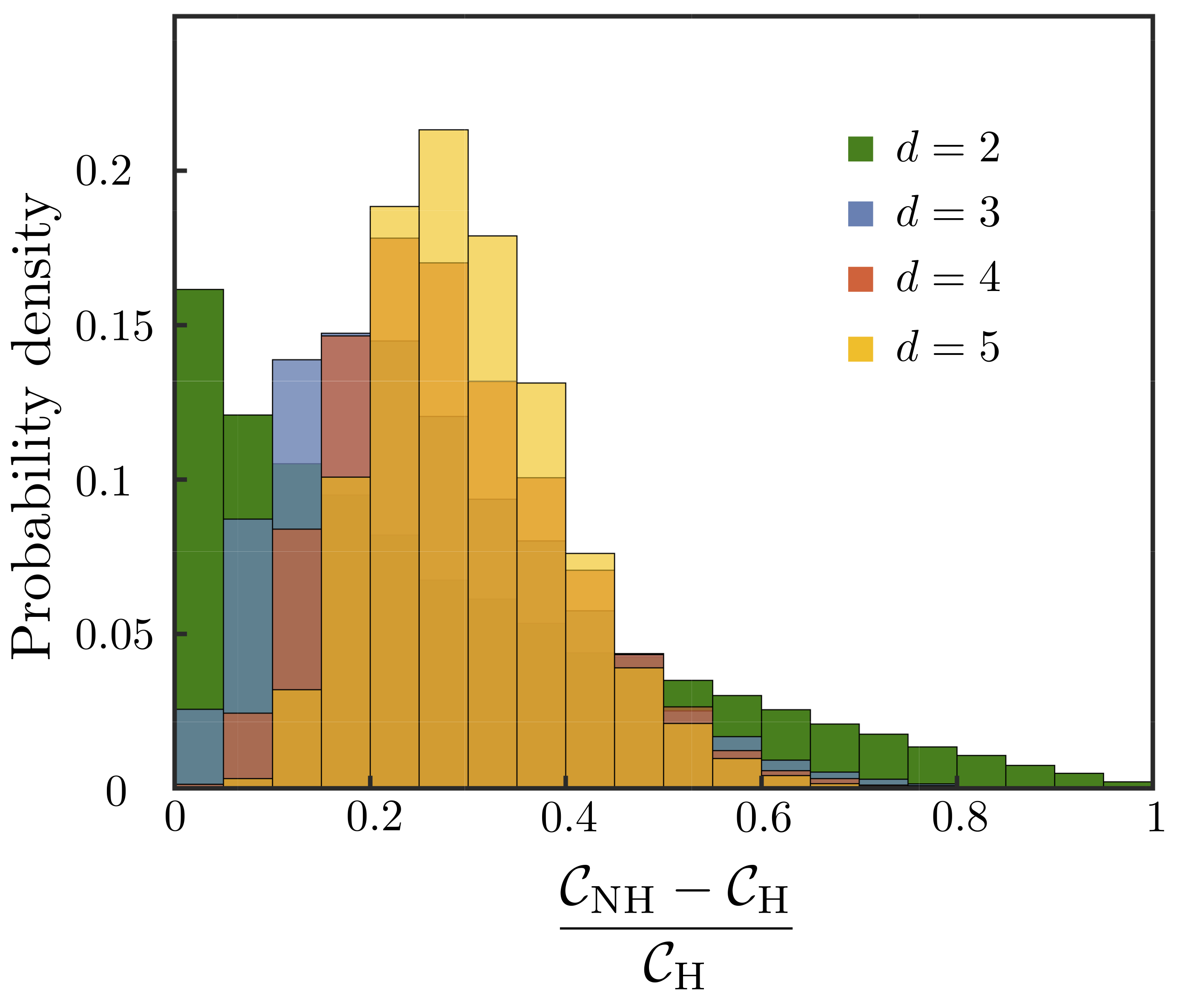
Figure 5: Gap between the HCRB and NCRB for two parameter estimation with random full rank probe states. We plot $(\mathcal{C}_{\text{N}}-\mathcal{C}_{\text{H}})/\mathcal{C}_{\text{H}}$ for random full rank probe states of different dimensions, up to and including dimensions of five. For each dimension 10,000 random probe states are shown.

VI Open problems and conjectures

Before concluding, we present some important questions that our work opens up.

VI.1 Does the gap persistence theorem hold for the NHCRB and HCRB?

An immediate question which arises from our work is whether or not theorem 10 can be extended to estimating three or more parameters. When the optimal estimator operator for the additional parameter to be estimated, $Z$, commutes with $(X,Y)$, the NHCRB reduces to a similar form as the NCRB and in this case our results from section III hold. More generally this will not necessarily be true. However, in Fig. 6, we provide numerical evidence that a weak gap persistence theorem may hold for the NHCRB and HCRB for estimating up to five parameters. For 190,000 Haar-random probe states, we did not find a single counter-example to this conjecture. However, this comes with the caveat that numerically we may not expect to find any examples where $\mathcal{C}_{\text{NH}}-\mathcal{C}_{\text{H}}\neq 0$ and $\mathcal{C}_{\text{NH}}(2)-\mathcal{C}_{\text{H}}(2)=0$, even if such an example existed.

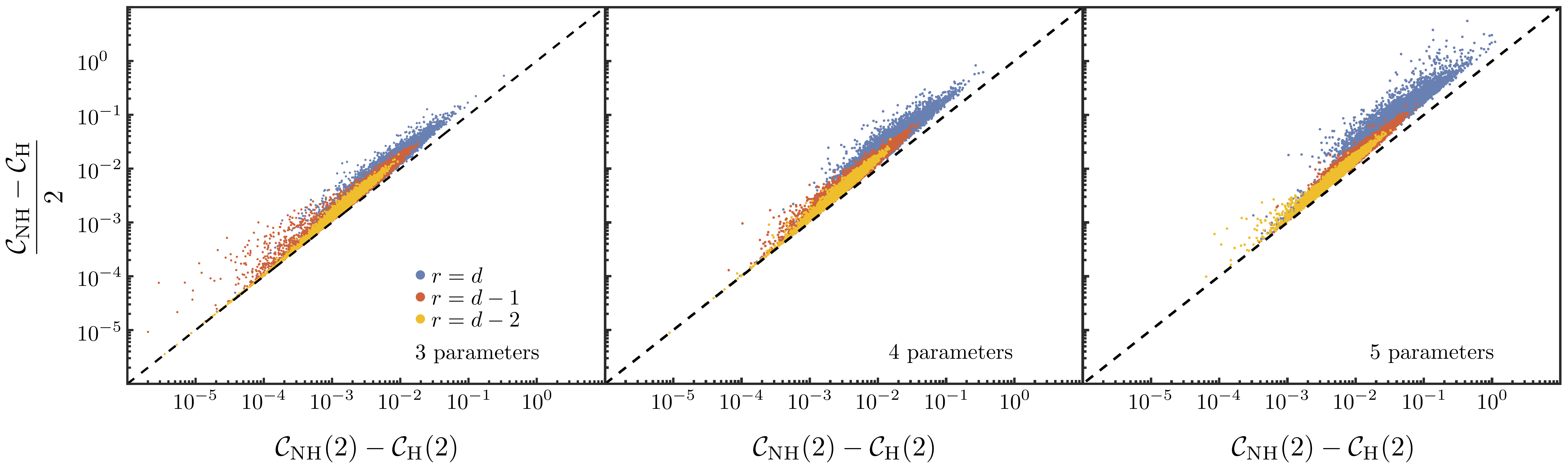
Figure 6: Numerical evidence that the gap persistence theorem for the HCRB and NCRB, theorem 10, may hold for estimating more than two parameters. We plot $(\mathcal{C}_{\text{NH}}-\mathcal{C}_{\text{H}})/2$ against $\mathcal{C}_{\text{NH}}(2)-\mathcal{C}_{\text{H}}(2)$ for random probe states of dimensions up to and including five ($d=3,4,5$) for estimating three, four and five parameters. For each dimension we include states of different rank, $r$. For each rank and dimension 10,000 random probe states were considered. The dashed black line shows $y=x$.

VI.2 When does the gap persistence theorem hold for the most informative bound?

Theorem 11 states that for estimating two parameters, a strong gap persistence theorem holds for the most informative bound and the HCRB. A natural question this opens up is whether this is true for estimating more than two parameters. Another open question is whether a gap persistence theorem holds for the most informative bound and the NHCRB. This is closely related to the attainability of the NHCRB, another important open question. If the NHCRB can always be saturated by a separable measurement, then this implies that the gap persistence theorem holds for the NHCRB and the most informative bound.

VI.3 Does the gap persistence theorem hold in other areas of quantum information?

Finally, we look more broadly and ask whether we can expect similar results to hold in other areas of quantum information where collective measurements are important. For example, in quantum state discrimination, it is known that collective measurements can help discriminate between mixed states Calsamiglia et al. (2010). For this task, the error probability for distinguishing two quantum states is given by the Helstrom bound Helstrom (1969) and the asymptotic error rate when allowing for infinitely many copies of the quantum state is given by the quantum Chernoff bound Nussbaum and Szkoła (2009); Audenaert et al. (2007). It may well be the case that some variation of the gap persistence theorem holds for the Helstrom bound and quantum Chernoff bound.

Even within quantum metrology, the gap persistence theorem may find use in slightly different settings. Recently, it was shown that many entangled states obtain their maximal metrological advantage over separable states when infinitely many copies of the state are available Trényi et al. (2022). In this scenario it may also be possible that such states cannot attain the maximal possible advantage with any finite number of copies of the probe state.

VII Discussions and conclusion

The SLDCRB and HCRB play a fundamental role in quantum metrology. However, given the experimental difficulty of performing collective measurements on even three copies of a probe state Conlon et al. (2022), our results suggest that for practical applications of quantum metrology the NCRB and NHCRB may be the more relevant quantities. By showing that there is a unique solution to the HCRB for two parameter estimation, we have been able to prove that the gap persistence theorem holds for the NCRB and HCRB and also for the most informative bound and the HCRB. Therefore, if the HCRB cannot be saturated with a single copy of the probe state, it cannot be saturated with measurements on any finite number of copies of the probe state. By extending our results to more general multiparameter estimation, we have provided a complete solution to a significant generalisation of one of five open problems in quantum information Horodecki et al. (2022). In theorems 13 and 16, we provide the necessary and sufficient conditions for the saturation of the SLDCRB with collective measurements on any finite number of copies of the probe state. This is done by showing that the gap persistence theorem holds for the NHCRB and SLDCRB.

We applied our results to show that for simultaneously estimating phase and phase diffusion, the HCRB can never be attained for any finite number of probe states. This result is easily generalised to many other important problems which can be mapped to qubit multiparameter estimation problems, such as quantum superresolution Chrostowski et al. (2017); Řehaček et al. (2017) or qubit tomography Hou et al. (2016); Razavian et al. (2020). Furthermore, this result can be extended to any scenario where the NCRB does not equal the HCRB for a single copy of the probe state Conlon et al. (2020); Friel et al. (2020). We anticipate that our results will have an important role to play in understanding the attainable precisions in quantum multiparameter estimation. While the benefits of the gap persistence theorem in quantum metrology are immediately obvious, the concept may prove beneficial for other areas of quantum information. Beyond quantum metrology, collective measurements are important in quantum illumination Zhuang et al. (2017), quantum communications Tserkis et al. (2020), entanglement distillation Bennett et al. (1996) and for better Bell inequality violations Liang and Doherty (2006). Future work will involve extending our results to these scenarios.

Note added: After concluding this work we became aware of Ref. Hayashi and Ouyang (2022). In this paper it was shown that for estimating four or more parameters the NHCRB is not necessarily a tight bound, although it is a good approximation to the most informative bound. This is related to some of the open questions we describe in section VI.

Appendix A Proof of basic results

A.1 Optimal $X$ matrices for two-copy HCRB

For simplicity we will denote the optimal estimator operators in the single-copy case as $X$ and $Y$, and in the two-copy case as $X_{2}$ and $Y_{2}$, given in Eq. (14). We now demonstrate that the two-copy estimator operators do in fact attain a HCRB which is half that of the single-copy case. First note that

$$\text{tr}\left\{S\otimes S(X_{2}^{2}+Y_{2}^{2})\right\}=\text{tr}\left\{S(X^{2}+Y^{2})\right\}/2\;,$$ (41)

i.e. the first term in the HCRB is two times smaller as expected. The second term in the HCRB is the sum of the eigenvalues of $\mathrm{i}(\sqrt{S}\otimes\sqrt{S})([X_{2},Y_{2}])(\sqrt{S}\otimes\sqrt{S})$. We can write

$$\begin{split}&\mathrm{i}(\sqrt{S}\otimes\sqrt{S})([X_{2},Y_{2}])(\sqrt{S}\otimes\sqrt{S})\\ =&\frac{\mathrm{i}}{4}(S\otimes(\sqrt{S}([X,Y])\sqrt{S})+(\sqrt{S}([X,Y])\sqrt{S})\otimes S)\;.\end{split}$$ (42)

The sum of the eigenvalues of the above matrix is given by the trace of this matrix. We then see that

$$\begin{split}&\text{tr}\{\mathrm{i}(\sqrt{S}\otimes\sqrt{S})([X_{2},Y_{2}])(\sqrt{S}\otimes\sqrt{S})\}\\ =&\frac{\mathrm{i}}{4}\text{tr}\{S\otimes(S[X,Y])+(S[X,Y])\otimes S\}\\ =&\frac{\mathrm{i}}{4}\text{tr}\left\{S[X,Y]\right\}+\frac{\mathrm{i}}{4}\text{tr}\left\{S[X,Y]\right\}\\ =&\frac{\mathrm{i}}{2}\text{tr}\left\{S[X,Y]\right\}\;.\end{split}$$ (43)

The second term in the HCRB is also a factor of two smaller confirming that the new matrices $X_{2}$ and $Y_{2}$ are indeed optimal for the two-copy case. Similarly, by direct substitution it can be easily verified that the matrices $X_{2}$ and $Y_{2}$ satisfy the unbiased conditions in the two-copy case. The extension to estimating $M$ copies is trivial. Note that this only proves that $\mathcal{C}_{\text{H}}(2)\leq\mathcal{C}_{\text{H}}/2$, as there could be some other matrices $X_{2}^{\prime}$ and $Y_{2}^{\prime}$, which give a lower bound. For the full proof of the additivity of the HCRB, we refer the reader to lemma 4 of Ref. Hayashi and Matsumoto (2008).

A.2 Subadditivity of the NCRB

Lemma 1 relates to the additivity of the HCRB, $\mathcal{C}_{\text{H}}(M)=\mathcal{C}_{\text{H}}/M$. However, for the NCRB, we have $\mathcal{C}_{\text{N}}(M)\leq\mathcal{C}_{\text{N}}/M$. We now show this to be true by evaluating $F_{\text{N}}(\mathbf{X}_{\text{N},2})$. From Appendix A.1 we know that the first term in the Nagaoka function evaluated with $\mathbf{X}_{\text{N},2}$ is exactly half of the corresponding term evaluated with $\mathbf{X}_{\text{N}}$. The second term in the Nagaoka function is

$$\begin{split}&\text{trAbs}\{S\otimes S[X_{2},Y_{2}]\}\\ =&\frac{1}{4}\text{trAbs}\{S[X,Y]\otimes S+S\otimes S[X,Y]\}\\ =&\frac{1}{4}\text{trAbs}\{S\otimes\sqrt{S}[X,Y]\sqrt{S}\\ &+\sqrt{S}[X,Y]\sqrt{S}\otimes S\}\\ \leq&\frac{1}{4}[\text{trAbs}\{S\otimes\sqrt{S}[X,Y]\sqrt{S}\}\\ &+\text{trAbs}\{\sqrt{S}[X,Y]\sqrt{S}\otimes S\}]\\ =&\frac{1}{2}\text{trAbs}\{\sqrt{S}[X,Y]\sqrt{S}\}\;,\end{split}$$ (44)

where the inequality follows from the sub-additive property of matrix norms, $\norm{A+B}\leq\norm{A}+\norm{B}$ Horn and Johnson (2012). We therefore arrive at $\mathcal{C}_{\text{N}}(2)\leq F_{\text{N}}(\mathbf{X}_{\text{N},2})\leq\mathcal{C}_{\text{N}}/2$. This argument can then be repeated many times to get the result for any $M$.

A.3 Proof of proposition 5

We first introduce an equivalence relation for linear operators

$$\begin{split}X&\sim_{S}X^{\prime}\iff\\ S(X-X^{\prime})=0\quad&\text{and}\quad(X-X^{\prime})S=0\;.\end{split}$$ (45)

If $\mathcal{L}(\mathcal{H})$ denotes the set of all matrices, this allows us to define a quotient space of $\mathcal{L}(\mathcal{H})$ as $\mathcal{L}^{\sim_{S}}(\mathcal{H})=\mathcal{L}(\mathcal{H})/\sim_{S}$. For rank deficient states, it is known that the SLD operators are not uniquely determined. However, the SLD operators are unique on the quotient space defined here Liu et al. (2014); Fujiwara and Nagaoka (1995).

For $Z=X+\mathrm{i}Y$ we note that the HCRB can be written as

$$\mathcal{C}_{\text{H}}=\min_{Z}\max\Big{\{}\tr{SZZ^{\dagger}},\tr{SZ^{\dagger}Z}\Big{\}}\,.$$ (46)

This function is strictly convex if $\tr{SZZ^{\dagger}}$ and $\tr{SZ^{\dagger}Z}$ are both strictly convex for $Z\in\mathcal{L}^{\sim_{S}}$. We now prove the strict convexity of $\tr{SZZ^{\dagger}}$ and $\tr{SZ^{\dagger}Z}$.

Proof. When $S$ is not full rank, we rely on the fact that minimisation in Eq. (46) is over $Z\in\mathcal{L}^{\sim_{S}}(\mathcal{H})$. We write $S$ in block matrix form such that only the upper diagonal block is non-zero

$$S=\begin{pmatrix}S_{r}&0\\ 0&0\end{pmatrix}\;,$$ (47)

where $S_{r}$ is a full rank matrix. We can write $Z$ as

$$Z=\begin{pmatrix}Z_{s}&Z_{sk}\\ Z_{ks}&Z_{k}\end{pmatrix}\;,$$ (48)

where the subscripts $s$ and $k$ refer to the support and kernel of $S$ respectively. We can then calculate $\tr{SZZ^{\dagger}}=\tr{S_{r}(Z_{s}Z_{s}^{\dagger}+Z_{sk}Z_{sk}^{\dagger})}>0$. Similarly $\tr{SZ^{\dagger}Z}=\tr{S_{r}(Z_{s}^{\dagger}Z_{s}+Z_{ks}^{\dagger}Z_{ks})}>0$.

To prove the strict convexity of the function $f(Z)=\text{tr}\{SZZ^{\dagger}\}$, we need to show that $f(tZ_{1}+(1-t)Z_{2})<tf(Z_{1})+(1-t)f(Z_{2})$, for $0<t<1$ and $Z_{1}\neq Z_{2}$. It is easy to show that $f(tZ_{1}+(1-t)Z_{2})-tf(Z_{1})-(1-t)f(Z_{2})$ is equal to

$$t(t-1)\text{tr}\{S(Z_{1}-Z_{2})(Z_{1}-Z_{2})^{\dagger}\}\;.$$ (49)

For the strict convexity of $f(Z)$ we require this expression to be negative. $t(t-1)<0$ for all $0<t<1$, but for arbitrary $Z_{1}$ and $Z_{2}$, the above expression is not strictly negative as $Z_{1}$ and $Z_{2}$ may differ only in the $Z_{k}$ elements, corresponding to the kernel of $S$. However, for $Z_{1}\neq Z_{2}$ and $Z_{1},Z_{2}\in\mathcal{L}^{\sim_{S}}(\mathcal{H})$ the expression is strictly negative, as shown above, showing that $f(Z)$ is strictly convex. Note that $Z_{1}=0$ or $Z_{2}=0$ is not allowed from the unbiased conditions.   

Hence, if there are two minimisers for Eq. (46), $Z_{1}$ and $Z_{2}$, they are equivalent.

We also note that similar arguments can be used to prove lemma 6, regarding the strict convexity of the SLDCRB. From Eq. (8) and the arguments above it is clear that the minimisation problem involved in computing the SLDCRB is minimising a sum of strictly convex functions, which is itself strictly convex.

Appendix B Proof of two parameter estimation results

B.1 Proof of theorem 10 in the $M$-copy case

First recall the optimal estimator operator in the $M$-copy case

$$\begin{split}X_{\text{H},M}&=\sum_{k=1}^{M}\frac{1}{M}X_{\text{H}}^{(k)}\;,\\ Y_{\text{H},M}&=\sum_{k=1}^{M}\frac{1}{M}Y_{\text{H}}^{(k)}\,.\end{split}$$ (50)

Using this, we now evaluate $A(\mathbf{X}_{\text{H},M})=\mathrm{i}\sqrt{S^{\otimes M}}[X_{\text{H},M},Y_{\text{H},M}]\sqrt{S^{\otimes M}}$ as

$$A(\mathbf{X}_{\text{H},M})=\frac{1}{M^{2}}\sum_{k=1}^{M}A^{k}_{S}(\mathbf{X}_{\text{H}})\;,$$ (51)

where $A^{k}_{S}(\mathbf{X}_{\text{H}})=S\otimes S\ldots\otimes A(\mathbf{X}_{\text{H}})\otimes\ldots S$, with $A(\mathbf{X}_{\text{H}})$ in the $k$th position. We now decompose this as $A(\mathbf{X}_{\text{H},M})=A_{+}(\mathbf{X}_{\text{H},M})-A_{-}(\mathbf{X}_{\text{H},M})$. For this we use $A^{k}_{S}(\mathbf{X}_{\text{H}})=A^{k}_{S+}(\mathbf{X}_{\text{H}})-A^{k}_{S-}(\mathbf{X}_{\text{H}})$, where $A^{k}_{S+}(\mathbf{X}_{\text{H}})=S\otimes S\ldots\otimes A_{+}(\mathbf{X}_{\text{H}})\otimes\ldots S$ and $A^{k}_{S-}(\mathbf{X}_{\text{H}})=S\otimes S\ldots\otimes A_{-}(\mathbf{X}_{\text{H}})\otimes\ldots S$. This gives

$$A(\mathbf{X}_{\text{H},M})=\frac{1}{M^{2}}\sum_{k=1}^{M}A^{k}_{S+}(\mathbf{X}_{\text{H}})-A^{k}_{S-}(\mathbf{X}_{\text{H}})\;.$$ (52)

Similarly to the main text, both $\text{tr}\{A^{k}_{S+}(\mathbf{X}_{\text{H}})\}>0$ and $\text{tr}\{A^{k}_{S-}(\mathbf{X}_{\text{H}})\}>0$ as $\text{tr}\{A_{+}(\mathbf{X}_{\text{H}})\}\neq 0$ and $\text{tr}\{A_{-}(\mathbf{X}_{\text{H}})\}\neq 0$. This completes the alternative proof of theorem 10.

B.2 Proof of theorem 11.

To prove the strong gap persistence theorem holds for the most informative bound and the HCRB, by proposition 3, we only need to show that the weak gap persistence theorem holds. We do this by proving the contraposition of the weak gap persistence theorem. Hence, we need to show that for all $M>1$, $\mathcal{C}_{\text{MI}}(M)=\mathcal{C}_{\text{H}}(M)$ implies $\mathcal{C}_{\text{MI}}=\mathcal{C}_{\text{H}}$.

We suppose that for $M=2$ we have $\mathcal{C}_{\text{MI}}(2)=\mathcal{C}_{\text{N}}(2)=\mathcal{C}_{\text{H}}(2)$ ($M>2$ can be proved similarly). This implies that the optimisers for the two-copy NCRB can be written

$$X_{\text{N},2}=\sum_{k}\xi_{k}\Pi_{k}\;,$$ (53)

and

$$Y_{\text{N},2}=\sum_{k}\eta_{k}\Pi_{k}\;,$$ (54)

where $\xi_{k}$, $\eta_{k}$ and the $\Pi_{k}$ are the estimators and POVM elements chosen to saturate $\mathcal{C}_{\text{MI}}(2)$. From the Naimark extension, there exists a projective measurement on some extended Hilbert space such that

$$\tilde{X}_{\text{N},2}=\sum_{k}\xi_{k}E_{k}\;,$$ (55)

and

$$\tilde{Y}_{\text{N},2}=\sum_{k}\eta_{k}E_{k}\;,$$ (56)

where $E_{k}$ are a set of projectors such that $\text{Tr}\{(S\otimes S)\Pi_{k}\}=\text{Tr}\{(S\otimes S\otimes S_{0})E_{k}\}$, where $S\otimes S\otimes S_{0}$ lives in the extended Hilbert space and $S_{0}$ is some arbitrary ancilla state.

Now consider performing measurements on the system $(S\otimes S_{0})\otimes(S\otimes S_{0})$. Let us first define a swap unitary which swaps the first two modes so that

$$U_{s}((S\otimes S_{0})\otimes(S\otimes S_{0}))U_{s}^{\dagger}=(S_{0}\otimes(S\otimes S\otimes S_{0}))\;.$$ (57)

Now consider acting with the projective measurement

$$E_{k}^{\prime}=U_{s}^{\dagger}\mathbb{I}\otimes E_{k}U_{s}$$ (58)

on the state $S\otimes S_{0}\otimes S\otimes S_{0}$. We have

$$\text{Tr}\{S\otimes S\otimes S_{0}E_{k}\}=\text{Tr}\{S\otimes S_{0}\otimes S\otimes S_{0}E_{k}^{\prime}\}\;.$$ (59)

Hence, any Naimark extension saturating $\mathcal{C}_{\text{MI}}(2)$ with ancilla states of the form $S\otimes S\otimes S_{0}$, can be converted to an extension using ancilla states of the form $S\otimes S_{0}\otimes S\otimes S_{0}$.

Now denote $S^{\prime}=S\otimes S_{0}$. For the state $S^{\prime}\otimes S^{\prime}$, we clearly have $\mathcal{C}_{\text{MI}}(2)=\mathcal{C}_{\text{NH}}(2)=\mathcal{C}_{\text{H}}(2)$. For this new state the optimiser for the NCRB can be written

$$X_{\text{N},2}^{\prime}=\frac{1}{2}X_{\text{H}}^{\prime}\otimes\mathbb{I}+\frac{1}{2}\mathbb{I}\otimes X_{\text{H}}^{\prime}\;,$$ (60)

and similarly for $Y_{\text{N},2}$ (This follows from $\mathcal{C}_{\text{NH}}(2)=\mathcal{C}_{\text{H}}(2)$). We know that $X_{\text{N},2}$ and $Y_{\text{N},2}$ can be decomposed into the same set of projective measurements. Hence, $[X_{\text{N},2},Y_{\text{N},2}]=0$. From the form of $X_{\text{N},2}$ and $Y_{\text{N},2}$, this implies $[X_{\text{N},1},Y_{\text{N},1}]=0$. Hence, the single copy observables can be measured simultaneously and so $\mathcal{C}_{\text{MI}}=\mathcal{C}_{\text{N}}=\mathcal{C}_{\text{H}}$.

We note that theorem 16 can be proven in a similar manner. In this case the strong gap persistence theorem between the NHCRB and the SLDCRB can be used to show that for all $M>1$, $\mathcal{C}_{\text{MI}}(M)=\mathcal{C}_{\text{SLD}}(M)$ implies $\mathcal{C}_{\text{MI}}=\mathcal{C}_{\text{SLD}}$. This in turn implies that a strong gap persistence theorem holds for the most informative bound and the SLDCRB.

B.3 Asymptotic equivalence of HCRB and NCRB

We now present the full proof of $\displaystyle\lim_{M\to\infty}M\mathcal{C}_{\text{N}}(M)=\mathcal{C}_{\text{H}}$. As $M\mathcal{C}_{\text{N}}(M)\geq M\mathcal{C}_{\text{H}}(M)=\mathcal{C}_{\text{H}}$, it is sufficient to prove

$$\lim_{M\to\infty}M\mathcal{C}_{\text{N}}(M)\leq\mathcal{C}_{\text{H}}\;.$$ (61)

For this we require the following lemma

Lemma 17 (Hayashi Hayashi (1999)).

Given a Hermitian matrix $X$ and a quantum state $S$, the following relations hold.

$$\begin{split}&\lim_{M\to\infty}\frac{1}{M}\text{tr}\{S^{\otimes M}\absolutevalue{X(M)}\}=\lim_{M\to\infty}\frac{1}{M}\text{trAbs}\{S^{\otimes M}X(M)\}\\ =&\lim_{M\to\infty}\frac{1}{M}\absolutevalue{\text{tr}\{S^{\otimes M}X(M)\}}=\absolutevalue{\text{tr}\{SX\}}\;,\end{split}$$ (62)

where $X(M)=\sum_{k=1}^{M}X^{(k)}$ with $X^{(k)}=\mathbb{I}\otimes\mathbb{I}\ldots\otimes X\otimes\ldots\otimes\mathbb{I}$, with $X$ in the $k$th position.

Proof (Lemma 17). Let $X=\sum_{a=1}^{d}x_{a}\ket{a}\bra{a}$ be an eigenvalue decomposition of $X$. By definition, we have

$$X^{(k)}=\sum_{a_{1},a_{2},\ldots a_{M}}x_{a_{k}}\ket{a_{1},a_{2},\ldots a_{M}}\bra{a_{1},a_{2},\ldots a_{M}}\;,$$ (63)

where $\sum\ket{a_{k}}\bra{a_{k}}=\mathbb{I}$. Using this we can write

$$X(M) =\sum_{a_{1},a_{2},\ldots a_{M}}\sum_{k=1}^{M}x_{a_{k}}\ket{a_{1},a_{2},\ldots a_{M}}\bra{a_{1},a_{2},\ldots a_{M}}$$ (64)

$$\absolutevalue{X(M)} =\sum_{a_{1},a_{2},\ldots a_{M}}\absolutevalue{\sum_{k=1}^{M}x_{a_{k}}}\ket{a_{1},a_{2},\ldots a_{M}}\bra{a_{1},a_{2},\ldots a_{M}}\;.$$ (65)

We next define $p(a):=\text{tr}\{S\ket{a}\bra{a}\}=\bra{a}S\ket{a}$, so that $p(a)$ forms a probability distribution. The expectation value of $S^{\otimes M}$ with respect to the state $\ket{a_{1},a_{2},\ldots a_{M}}$ leads to the i.i.d. distribution of $p(a)$.

$$\begin{split}&\bra{a_{1},a_{2},\ldots a_{M}}S^{\otimes M}\ket{a_{1},a_{2},\ldots a_{M}}\\ &=\prod_{k=1}^{M}p(a_{k})=:p_{M}(a_{1},a_{2},\ldots,a_{M})\;.\end{split}$$ (66)

We can then get the following result

$$\begin{split}\frac{1}{M}\text{tr}\{S^{\otimes M}\absolutevalue{X(M)}\}&=\frac{1}{M}\sum_{a_{1},a_{2},\ldots a_{M}}\absolutevalue{\sum_{k=1}^{M}x_{a_{k}}}\prod_{k=1}^{M}p(a_{k})\\ &=\frac{1}{M}E_{p_{M}}\bigg{[}\absolutevalue{\sum_{k=1}^{M}X_{a_{k}}}\bigg{]}\\ &\to\absolutevalue{E_{p}[X]}\quad(M\to\infty)\\ &=\absolutevalue{\text{tr}\{SX\}}\;,\end{split}$$ (67)

where the third line follows from the law of large numbers and the dominated convergence theorem. We can apply the dominated convergence theorem as $\absolutevalue{\sum_{k=1}^{M}X_{a_{k}}}/M$ is bounded. This shows $\lim\limits_{M\to\infty}\frac{1}{M}\text{tr}\{S^{\otimes M}\absolutevalue{X(M)}\}=\absolutevalue{\text{tr}\{SX\}}$. To prove the remaining relations we use the following inequalities

$$\text{tr}\{\sqrt{S}\absolutevalue{X}\sqrt{S}\}\geq\text{tr}\{\absolutevalue{\sqrt{S}X\sqrt{S}}\}\geq\absolutevalue{\text{tr}\{\sqrt{S}X\sqrt{S}\}}\;.$$ (68)

Using the identity $\text{trAbs}\{SX\}=\text{tr}\{\absolutevalue{\sqrt{S}X\sqrt{S}}\}$, Eq. (LABEL:eqs:hayashilemma) is proven.

 

Using this lemma, we now prove

$$\lim_{M\to\infty}MF_{\text{N}}(\mathbf{X}_{M})=F_{\text{H}}(\mathbf{X})\;,$$ (69)

for any $\mathbf{X}\in\mathcal{L}(\mathcal{H})^{2}$. We have

$$\begin{split}MF_{\text{N}}(\mathbf{X}_{M})&=MF_{\text{S}}(\mathbf{X}_{M})+M\text{trAbs}\{S^{\otimes M}\mathrm{i}[X_{M},Y_{M}]\}\\ &=F_{\text{S}}(\mathbf{X})+\frac{1}{M}\text{trAbs}\{S^{\otimes M}\mathrm{i}[X(M),Y(M)]\}\;.\end{split}$$ (70)

By lemma 17, the second term converges to $\absolutevalue{\text{tr}\{S\mathrm{i}[X,Y]\}}$, in the limit $M\to\infty$. Therefore Eq. (69) is proven.

Finally, we prove Eq. (61).

$$M\mathcal{C}_{\text{N}}(M)=MF_{\text{N}}(\mathbf{X}_{N,M})\leq MF_{\text{N}}(\mathbf{X}_{H,M})\;.$$ (71)

This final term tends to $F_{\text{H}}(\mathbf{X}_{H})=\mathcal{C}_{\text{H}}$ as $M\to\infty$. Hence, when performing a collective measurement on infinitely many copies of the probe state the HCRB and NCRB are equal as expected.

B.4 Equivalence of the HCRB and NCRB for pure states

Matsumoto proved that for pure states, $\mathcal{C}_{\text{H}}=\mathcal{C}_{\text{MI}}$ Matsumoto (2002), which implies $\mathcal{C}_{\text{H}}=\mathcal{C}_{\text{N}}$. We now prove that $\mathcal{C}_{\text{H}}=\mathcal{C}_{\text{N}}$, consistent with Matsumoto’s result. For a pure state we can write $S=\ket{\psi}\bra{\psi}$. Then $A(\mathbf{X})=\mathrm{i}\sqrt{S}[X,Y]\sqrt{S}$ has at most one non-zero eigenvalue for all $\mathbf{X}$. Hence, either $A_{+}(\mathbf{X})=0$ or $A_{-}(\mathbf{X})=0$. Lemma 4 then implies $\mathcal{C}_{\text{H}}=\mathcal{C}_{\text{N}}$. However, this does not prove $\mathcal{C}_{\text{H}}=\mathcal{C}_{\text{MI}}$, only the weaker statement that $\mathcal{C}_{\text{H}}=\mathcal{C}_{\text{N}}$.

Appendix C Proof of multiparameter estimation results

C.1 Re-writing the Nagaoka–Hayashi function

Lemma 18 (Hayashi Hayashi (1999)).

The Nagaoka–Hayashi function can be written as

$$F_{\text{NH}}[\mathbf{X}|W]=\text{tr}\{W\real Z[\mathbf{X}]\}+A^{\text{NH}}_{-}[\mathbf{X}|W],$$ (72)

where $Z[\mathbf{X}]$ and $A^{\text{NH}}_{-}[\mathbf{X}|W]$ are defined in the text.

Proof (Lemma 18). Define the symmetrized matrix of ${\mathbb{X}}$ by $s({\mathbb{X}})$. Explicitly, for ${\mathbb{X}}=[{\mathbb{X}}_{ij}]$ with ${\mathbb{X}}_{ij}\in{\cal L}({\cal H})$, $s({\mathbb{X}})=\frac{1}{2}({\mathbb{X}}_{ij}+{\mathbb{X}}_{ji})$. Then, the identity ${\mathbb{X}}=s({\mathbb{X}})+a({\mathbb{X}})$ holds. We next rewrite the Nagaoka–Hayashi function as follows.

$$\begin{split}F_{\text{NH}}[\mathbf{X}|W]=&\min_{{\mathbb{L}}^{\prime}}\{\mathbb{T}\mathrm{r}\{{\mathbb{W}}\,{\mathbb{S}}\,s(\mathbf{X}\mathbf{X}^{\intercal})\}+\mathbb{T}\mathrm{r}\{{\mathbb{W}}{\mathbb{S}}{\mathbb{L}}^{\prime}\}\,|\\ &\qquad{\mathbb{L}}^{\prime}\geq a(\mathbf{X}\mathbf{X}^{\intercal}),\,{\mathbb{L}}^{\prime}_{ij}={\mathbb{L}}^{\prime}_{ji}\mbox{: Hermitian}\}\end{split}$$ (73)

$$\begin{split}=&\text{tr}\{W\real Z[\mathbf{X}]\}+\min_{{\mathbb{L}}^{\prime}}\{\mathbb{T}\mathrm{r}\{{\mathbb{W}}{\mathbb{S}}{\mathbb{L}}^{\prime}\}\,|\\ &\qquad{\mathbb{L}}^{\prime}\geq a(\mathbf{X}\mathbf{X}^{\intercal}),\,{\mathbb{L}}^{\prime}_{ij}={\mathbb{L}}^{\prime}_{ji}\mbox{: Hermitian}\}\end{split}$$ (74)

$$\begin{split}=&\text{tr}\{W\real Z[\mathbf{X}]\}+\\ &\min_{{\mathbb{V}}}\{\mathbb{T}\mathrm{r}\{{\mathbb{V}}\}\,|\,{\mathbb{V}}\geq({\mathbb{W}}{\mathbb{S}})^{1/2}a(\mathbf{X}\mathbf{X}^{\intercal})({\mathbb{W}}{\mathbb{S}})^{1/2},\\ &\qquad\qquad{\mathbb{V}}_{ij}={\mathbb{V}}_{ji}\mbox{: Hermitian}\}\end{split}$$ (75)

$$\begin{split}=&\text{tr}\{W\real Z[\mathbf{X}]\}+\\ &\min_{{\mathbb{V}}^{\prime}}\{\mathbb{T}\mathrm{r}\{{\mathbb{V}}^{\prime}\}\,|\,{\mathbb{V}}^{\prime}\geq 0,\\ &\quad a({\mathbb{V}}^{\prime})-({\mathbb{W}}{\mathbb{S}})^{1/2}a(\mathbf{X}\mathbf{X}^{\intercal})({\mathbb{W}}{\mathbb{S}})^{1/2}=0\}\;.\end{split}$$ (76)

The first line follows by setting ${\mathbb{L}}=s(\mathbf{X}\mathbf{X}^{\intercal})+{\mathbb{L}}^{\prime}$. The second line holds by the definition of the $Z[\mathbf{X}]$ matrix. The third line is obtained by introducing a new variable ${\mathbb{V}}:=({\mathbb{W}}{\mathbb{S}})^{1/2}{\mathbb{L}}^{\prime}({\mathbb{W}}{\mathbb{S}})^{1/2}$. To get the final line, we set ${\mathbb{V}}^{\prime}={\mathbb{V}}-({\mathbb{W}}{\mathbb{S}})^{1/2}a(\mathbf{X}\mathbf{X}^{\intercal})({\mathbb{W}}{\mathbb{S}})^{1/2}$, and use the fact that $({\mathbb{W}}{\mathbb{S}})^{1/2}a(\mathbf{X}\mathbf{X}^{\intercal})({\mathbb{W}}{\mathbb{S}})^{1/2}$ is Hermitian and the antisymmetrized matrix of ${\mathbb{V}}^{\prime}$ is equal to it. We remark that this new variable ${\mathbb{V}}^{\prime}$ does not necessarily satisfy the condition ${\mathbb{V}}^{\prime}_{ij}={\mathbb{V}}^{\prime}_{ji}$.   

C.2 Proof of theorem 13

Proof (Theorem 13). As mentioned in the main text, we will prove the theorem by the chain: i) $\Rightarrow$ ii) $\Rightarrow$ iii) $\Rightarrow$ iv) $\Rightarrow$ i). We prove iii) $\Rightarrow$ iv) and iv) $\Rightarrow$ i) below.

Proof that iii) $\Rightarrow$ iv):
We assume condition iii). $\mathcal{C}_{\text{NH}}[\mathbb{I}]=\mathcal{C}_{\text{S}}[\mathbb{I}]$ implies

$$\begin{split}\min_{\mathbf{X}}\{F_{\text{NH}}&[\mathbf{X}]\,|\,X_{i}:\,\mathrm{l.u.}\text{ }\mathrm{and}\text{ }\mathrm{Hermitian}\}=\mathcal{C}_{\text{S}}=\text{tr}\{{J_{S}}^{-1}\}\\ \Leftrightarrow\min_{\mathbf{X}}\{&\text{tr}\{\real Z[\mathbf{X}]\}+A^{\text{NH}}_{-}[\mathbf{X}]\,|\,\\ &X_{i}:\,\mathrm{l.u.}\text{ }\mathrm{and}\text{ }\mathrm{Hermitian}\}=\text{tr}\{\real Z[\mathbf{X}_{\text{S}}]\}\;,\end{split}$$ (77)

where $\mathbf{X}_{\text{S}}$ denotes the optimal $\mathbf{X}$ which minimises the first term of the Nagaoka–Hayashi function. Explicitly, $\mathbf{X}_{\text{S}}=(X_{\text{S},i})=(L^{i})$ with $L^{i}:=\sum_{j}({J_{S}}^{-1})_{ji}L_{j}$.

Lemma 6 shows that the function $\text{tr}\{\real Z[\mathbf{X}]\}$ is strictly convex about $\mathbf{X}$ (on the quotient space when $S$ is not full rank) and the optimiser exists uniquely. By definition, it holds that the second term $A^{\text{NH}}_{-}[\mathbf{X}]$ is non-negative function of $\mathbf{X}$. We can apply lemma 19 (Appendix C.3) to show that this is possible if and only if the following condition holds.

$$A^{\text{NH}}_{-}[\mathbf{X}_{\text{S}}]=0\;.$$ (78)

$\mathbb{T}\mathrm{r}\{{\mathbb{V}}\}=0$ holds if and only if ${\mathbb{V}}=0$ for a positive matrix ${\mathbb{V}}$. This is possible if and only if ${\mathbb{S}}^{1/2}a(\mathbf{X}_{\text{S}}\mathbf{X}_{\text{S}}^{\intercal}){\mathbb{S}}^{1/2}=0$ is true, since this matrix is Hermitian. Therefore, it is equivalent to the condition such that all elements are zero. In other words, we have

$$\forall i,j,\,\sqrt{S}[L^{i}\,,\,L^{j}]\sqrt{S}=0\ \Leftrightarrow\ \forall i,j,\,\sqrt{S}[L_{i}\,,\,L_{j}]\sqrt{S}=0\;.$$ (79)

It is straightforward to see this is also equivalent to

$$\forall i,j,\,\text{trAbs}\{S[L_{i}\,,\,L_{j}]\}=0\;,$$ (80)

or using our alternative notation $\forall i,j,\,\text{trAbs}\{S[X_{\text{S},i}\,,\,X_{\text{S},j}]\}=0$. When $S$ is full rank, this immediately proves $[L_{i}\,,\,L_{j}]=0,\,\forall i,j$. Thus, we do not need to consider any extension of the Hilbert space.

If $S$ is rank deficient, note that the optimizer $X_{\text{NH}}$ also needs to satisfy the following condition from $\mathcal{C}_{\text{NH}}[\mathbb{I}]=\mathcal{C}_{\text{S}}[\mathbb{I}]$

$$X_{\text{NH},i}=L^{i}\mbox{ up to equivalence }\sim_{S},\,\forall i.$$ (81)

Let $\Pi=\{\Pi_{k}\}$ and $\hat{\theta}$ be an optimal POVM and estimator, then $\mathcal{C}_{\text{MI}}[\mathbb{I}]=\mathcal{C}_{\text{NH}}[\mathbb{I}]$ implies that the optimiser for the NHCRB can be decomposed into some POVM

$$X_{\text{NH},i}=\sum_{k}(\hat{\theta}_{i}(k)-\theta_{i})\Pi_{k}\;.$$ (82)

Combining the above two relations, after some algebra we get

$$L_{i}=\sum_{k}\ell_{i}(k)\Pi_{k}\mbox{ up to equivalence }\sim_{S},\,\forall i,$$ (83)

where $\ell_{i}(k):=\sum_{j}J_{\text{S},ji}(\hat{\theta}_{j}(k)-\theta_{j})$. With this expression we can apply the Naimark extension to find a larger Hilbert space in which the POVM elements are expressed as mutually orthogonal projectors Neumark (1943). After this extension, the SLDs $\tilde{L}_{i}$ commute with each other.

iv) $\Rightarrow$ i):
Suppose we find such an extension where the SLDs $\tilde{L}_{i}$ for the extended model $\tilde{S}_{\theta}=U(S_{\theta}\otimes S_{0})U^{\dagger}$ are commutative. We can diagonalize all $\tilde{L}_{i}$ simultaneously as

$$\tilde{L}_{i}=\sum_{k}\ell_{i}(k)E_{k}\;,$$ (84)

where $\{E_{k}\}$ are mutually orthogonal projectors. When $S$ is not full rank, we can always extend $\{E_{k}\}$ to form a projection measurement. By substituting into the SLD equation, we explicitly obtain $\ell_{i}(k)$ as

$$\ell_{i}(k)=\frac{\text{tr}\{\tilde{S}_{i}E_{k}\}}{\text{tr}\{\tilde{S}E_{k}\}}\;,$$ (85)

which is the score function. We define $\ell_{i}(k)=0$ when $\text{tr}\{\tilde{S}E_{k}\}=0$. Thus, $\sum_{k}\ell_{i}(k)\ell_{j}(k)\text{tr}\{\tilde{S}E_{k}\}=J_{S,ij}$ holds. Note that the SLD Fisher information remains invariant under the extension (see e.g. proposition 2.1 of Ref. Liu et al. (2019)). Under this circumstance, an optimal measurement is given by $\{E_{k}\}$ and a locally unbiased estimator is constructed by

$$\hat{\theta}_{i}(k)=\theta_{i}+\sum_{j}(J_{S}^{-1})_{ji}\ell_{j}(k)\;.$$ (86)

Finally, we calculate the MSE matrix to show that this is equal to the inverse of the SLD Fisher information matrix. From Eq. (17), we have

$$\begin{split}V_{ij}&=\sum_{k}\big{(}\sum_{m}(J_{S}^{-1})_{mi}\ell_{m}(k)\big{)}\big{(}\sum_{n}(J_{S}^{-1})_{nj}\ell_{n}(k)\big{)}\text{tr}\{\tilde{S}E_{k}\}\\ &=\sum_{m}(J_{S}^{-1})_{mi}\sum_{n}(J_{S}^{-1})_{nj}(J_{S})_{mn}\\ &=(J_{S}^{-1})_{ji}\;,\end{split}$$ (87)

where we use the fact that $\sum_{n}(J_{S}^{-1})_{nj}(J_{S})_{mn}=\delta_{jm}$, which follows from $(J_{S})(J_{S})^{-1}=\mathbb{I}$.   

Note that in proving iii) $\Rightarrow$ iv), being able to decompose the $L^{i}$ in terms of some POVM as

$$L^{i}=\sum_{k}(\hat{\theta}^{\prime}_{i}(k)-\theta_{i})\Pi_{k}\;,$$ (88)

does not necessarily imply that $\tilde{L}_{i}$ can be decomposed into projective measurements. This is because the Naimark extension of $L^{i}$ does not necessarily satisfy the conditions to be an SLD operator i.e., this decomposition does not imply $\mathcal{C}_{\text{MI}}[\mathbb{I}]=\mathcal{C}_{\text{NH}}[\mathbb{I}]=\mathcal{C}_{\text{S}}[\mathbb{I}]$. The Naimark extension will always exist for $L^{i}$ of this form, however it is not necessarily identical to the SLD operators on the extended space, $\tilde{L}_{i}$. See Ref. Conlon et al. (2022) for an example of this form. Further details on this will be presented in future work.

C.3 Lemma to support theorem 13

Lemma 19.

Consider the sum of two non-negative functions $f(x)=f_{1}(x)+f_{2}(x)$ on the domain ${\cal X}$. Suppose the optimization of $f_{1}$ under a constraint $C$ exists and the optimiser is unique, then the following statement holds.

$$\begin{split}&\min_{x\in{\cal X}:\,C}f(x)=\min_{x\in{\cal X}:\,C}f_{1}(x)\ \\ \Leftrightarrow\ &f_{2}(x_{*})=0\mbox{ with }x_{*}:=\arg\min_{x\in{\cal X}:\,C}f_{1}(x)\end{split}$$ (89)

Appendix D Simultaneous estimation of phase and phase diffusion

D.1 Analytic solution to the HCRB and NCRB for simultaneously estimating phase and phase diffusion

We first note that the possible solutions to the HCRB and NCRB are greatly restricted by the unbiased conditions for this problem. This makes an explicit optimisation of the matrices $\mathbf{X}$ feasible for this problem. However, it is considerably simpler to use the results of Ref. Suzuki (2016) and Ref. Gill and Massar (2000) to obtain analytic expressions for the HCRB and NCRB respectively. Ref. Suzuki (2016) provides a simple method for obtaining an analytic form for the HCRB, which only requires that we evaluate the SLD and right logarithmic derivative (RLD) operators. In what follows we set $\phi=0$ as the HCRB has no $\phi$ dependence. The SLD operators are given by

$$L_{\phi}=\mathrm{i}\text{e}^{-\delta^{2}}\text{sin}(\lambda)\begin{pmatrix}0&-1\\ 1&0\end{pmatrix}\;,$$ (90)

and

$$L_{\delta}=\begin{pmatrix}L_{\delta,11}&L_{\delta,12}\\ L_{\delta,21}&L_{\delta,22}\end{pmatrix}\;,$$ (91)

where

$$\begin{split}L_{\delta,11}&=\delta(1-\text{cos}(\lambda))(-1+\text{coth}(\delta^{2}))\\ L_{\delta,12}&=\mathcal{L}_{\delta,21}=-\delta\text{cosech}(\delta^{2})\text{sin}(\lambda)\\ L_{\delta,22}&=\delta(1+\text{cos}(\lambda))(-1+\text{coth}(\delta^{2}))\;.\end{split}$$ (92)

The RLD operator for estimating $\phi$ is given by

$$\tilde{\mathcal{L}}_{\phi}=\begin{pmatrix}\tilde{\mathcal{L}}_{\phi,11}&\tilde{\mathcal{L}}_{\phi,12}\\ \tilde{\mathcal{L}}_{\phi,21}&\tilde{\mathcal{L}}_{\phi,22}\end{pmatrix}\;,$$ (93)

where

$$\begin{split}\tilde{\mathcal{L}}_{\phi,11}&=-\frac{\mathrm{i}}{2}(-1+\text{coth}(\delta^{2}))\\ \tilde{\mathcal{L}}_{\phi,12}&=-\tilde{\mathcal{L}}_{\phi,21}=-\frac{\mathrm{i}}{2}\text{cosech}(\delta^{2})\text{tan}(\lambda/2)\\ \tilde{\mathcal{L}}_{\phi,22}&=\frac{\mathrm{i}}{2}(-1+\text{coth}(\delta^{2}))\;.\end{split}$$ (94)

The RLD operator for estimating $\delta$ is given by

$$\tilde{\mathcal{L}}_{\delta}=\begin{pmatrix}\tilde{\mathcal{L}}_{\delta,11}&\tilde{\mathcal{L}}_{\delta,12}\\ \tilde{\mathcal{L}}_{\delta,21}&\tilde{\mathcal{L}}_{\delta,22}\end{pmatrix}\;,$$ (95)

where

$$\begin{split}\tilde{\mathcal{L}}_{\delta,11}&=\delta(-1+\text{coth}(\delta^{2}))\\ \tilde{\mathcal{L}}_{\delta,12}&=\mathcal{L}_{\delta,21}=-\delta\text{cosech}(\delta^{2})\text{tan}(\lambda/2)\\ \tilde{\mathcal{L}}_{\delta,22}&=\delta(-1+\text{coth}(\delta^{2}))\;.\end{split}$$ (96)

Theorem 1 of Ref. Suzuki (2016) gives two analytic forms of the HCRB. One of these forms depends on the RLD Cramér-Rao bound, given by

$$\mathcal{C}_{\text{R}}=\frac{(\text{e}^{2\delta^{2}}-1)(1+4\delta^{2}+4\delta\absolutevalue{\text{cos}(\lambda)})}{4\delta^{2}\text{sin}(\lambda)^{2}}\;.$$ (97)

To give the HCRB, we define the following function

$$\beta=1-\frac{(-1+\text{e}^{2\delta^{2}})\absolutevalue{\text{cos}(\lambda)}}{2\delta}\\$$ (98)

Theorem 1 of Ref. Suzuki (2016) gives the HCRB as

$$\mathcal{C}_{\text{H}}=\begin{cases}\mathcal{C}_{\text{R}}&\text{ if }\beta\leq 0\\ \gamma&\text{ if }\beta\geq 0\end{cases}$$ (99)

where

$$\gamma=\frac{-1+e^{4\delta^{2}}+8e^{2\delta^{2}}\delta^{2}+\text{cos}(2\lambda)(-1+e^{2\delta^{2}})^{2}}{8\delta^{2}\text{sin}(\lambda)^{2}}\;.$$ (100)

There is a smooth transition between the different solutions to the HCRB in Eq. (99) when $\beta$ changes sign.

Using Ref. Gill and Massar (2000) we can also solve the NCRB. For a qubit model the NCRB is given by

$$\mathcal{C}_{\text{N}}=(\text{tr}\{J_{\text{S}}^{-1/2}\})^{2}\;,$$ (101)

where $J_{\text{S}}$ is the SLD Fisher information matrix, which can be calculated from the SLD operators. This gives a NCRB of

$$\mathcal{C}_{\text{N}}=\frac{\text{e}^{2\delta^{2}}}{\text{sin}^{2}(\lambda)}\big{(}1+\frac{1-\text{e}^{-2\delta^{2}}}{4\delta^{2}}+\frac{\sqrt{1-\text{e}^{-2\delta^{2}}}}{\delta}\big{)}\;.$$ (102)

D.2 Proof of a strict inequality between the NCRB and HCRB

We now wish to show that the two bounds derived in the previous section obey a strict inequality, $\mathcal{C}_{\text{N}}>\mathcal{C}_{\text{H}}$. Consider first when $\beta\leq 0$, we can write

$$\delta\leq\frac{1}{2}(-1+\text{e}^{2\delta^{2}})\absolutevalue{\text{cos}(\lambda)}\;.$$ (103)

The difference between the two bounds is given by

$$\mathcal{C}_{\text{N}}-\mathcal{C}_{\text{H}}=\frac{4(\text{e}^{2\delta^{2}}\sqrt{1-\text{e}^{-2\delta^{2}}}+\delta-(-1+\text{e}^{2\delta^{2}})\absolutevalue{\text{cos}(\lambda)})}{4\delta\text{sin}(\lambda)^{2}}\;.$$ (104)

Note that $\mathcal{C}_{\text{N}}-\mathcal{C}_{\text{H}}>0$ is equivalent to

$$\sqrt{1-\text{e}^{-2\delta^{2}}}+\text{e}^{-2\delta^{2}}\delta-(1-\text{e}^{-2\delta^{2}})\absolutevalue{\text{cos}(\lambda)})>0\;,$$ (105)

where we have simply removed terms which are guaranteed to be positive for $\delta>0$. We use the substitution $x=\sqrt{1-\text{e}^{-2\delta^{2}}}$ and $a=\absolutevalue{\text{cos}(\lambda)}$. Then we can rewrite the above expression as

$$\begin{split}&x+\text{e}^{-2\delta^{2}}\delta-ax^{2}\\ =&x(1-ax)+\text{e}^{-2\delta^{2}}\delta\;.\end{split}$$ (106)

We note that $f(x)=x(1-ax)$ is guaranteed to be positive for $0<x<1$ (which is satisfied for $\delta>0$) and $a=\absolutevalue{\text{cos}(\lambda)}$. As $\text{e}^{-2\delta^{2}}\delta$ is also guaranteed to be positive, we can conclude that in this case there is a non-zero gap between the NCRB and HCRB.

We now consider the second possibility when $\beta\geq 0$.

$$\begin{split}2\delta&\geq(-1+\text{e}^{2\delta^{2}})\absolutevalue{\text{cos}(\lambda)}\\ &\geq(-1+\text{e}^{2\delta^{2}})\text{cos}(\lambda)\;.\end{split}$$ (107)

The difference between the two bounds in this case is given by

$$\begin{split}\mathcal{C}_{\text{N}}-\mathcal{C}_{\text{H}}=\frac{-1}{8\delta^{2}\text{sin}(\lambda)^{2}}\bigg{(}&1+\text{e}^{4\delta^{2}}-2\text{e}^{2\delta^{2}}(1+4\sqrt{1-\text{e}^{-2\delta^{2}}}\delta)\\ &+(2\text{cos}(\lambda)^{2}-1)(-1+\text{e}^{2\delta^{2}})^{2}\bigg{)}\;.\end{split}$$ (108)

As above, we drop any terms with definite positive sign, and using Eq. (107), we find that $\mathcal{C}_{\text{N}}-\mathcal{C}_{\text{H}}>0$ is equivalent to

$$8\delta(\text{e}^{2\delta^{2}}\sqrt{1-\text{e}^{-2\delta^{2}}}-\delta)>0\;.$$ (109)

As before, we shall attempt to prove that this term is strictly positive. Using the substitution $x=2\delta^{2}$, we see that our aim is to show

$$\text{e}^{x}\sqrt{1-\text{e}^{-x}}>\sqrt{\frac{x}{2}}\;.$$ (110)

As both sides of this inequality are positive (for $\delta>0$), we can square both sides, so that we wish to show

$$\text{e}^{2x}(1-\text{e}^{-x})-\frac{x}{2}>0\;,$$ (111)

for $x>0$. This quantity evaluated at $x=0$ gives 0, hence our aim is simply to show that Eq. (111) is monotonically increasing for $x>0$. The derivative of Eq. (111) is $-\frac{1}{2}-\text{e}^{x}+2\text{e}^{2x}$, which is positive for $x>0$. Hence, we also have $\mathcal{C}_{\text{N}}>\mathcal{C}_{\text{H}}$ when $\beta\geq 0$.

D.3 Lower bound on $F_{\text{N}}(\mathbf{X}_{\text{H},M})$

When analysing the simultaneous estimation of phase and phase diffusion, we wish to show $F_{\text{N}}(\mathbf{X}_{\text{H},M})>F_{\text{H}}(\mathbf{X}_{\text{H},M})$. However, even though the form of $\mathbf{X}_{\text{H},M}$ is known analytically, evaluating $F_{\text{N}}(\mathbf{X}_{\text{H},M})$ for large $M$ is still computationally expensive. To circumvent this, we provide a lower bound, $B_{M}$, on $F_{\text{N}}(\mathbf{X}_{\text{H},M})$, so that $B_{M}\leq F_{\text{N}}(\mathbf{X}_{\text{H},M})$. This is useful as $B_{M}>F_{\text{H}}(\mathbf{X}_{\text{H},M})$ implies $F_{\text{N}}(\mathbf{X}_{\text{H},M})>F_{\text{H}}(\mathbf{X}_{\text{H},M})$.

Lemma 1 and Appendix A.1 show that $\mathcal{C}_{\text{H},M}=\mathcal{C}_{\text{H}}/M$. From this we can conclude that the first term in both $F_{\text{H}}(\mathbf{X}_{\text{H},M})$ and $F_{\text{N}}(\mathbf{X}_{\text{H},M})$ are equal to $\text{tr}\{S(X_{\text{H}}X_{\text{H}}+Y_{\text{H}}Y_{\text{H}})\}/M$, which is trivial to evaluate analytically for any $M$. For evaluating the second term in the NCRB we need to consider $\text{trAbs}\{A(\mathbf{X}_{\text{H}})\}$. The sum of the absolute values of the eigenvalues of $A(\mathbf{X}_{\text{H}})$ is equal to the nuclear norm, denoted $\norm{A(\mathbf{X}_{\text{H}})}_{*}$. For $M$ copies of the quantum state

$$\begin{split}&\norm{\sqrt{S^{\otimes M}}[X_{\text{H},M},Y_{\text{H},M}]\sqrt{S^{\otimes M}}}_{*}\\ =&\norm{S^{\otimes M}[X_{\text{H},M},Y_{\text{H},M}]}_{*}\\ =&\frac{1}{M^{2}}\Biggl{|}\!\Biggl{|}\!\,S^{\otimes M}\Biggl{[}\!\;\sum_{k=1}^{M}X_{\text{H}}^{(k)}\sum_{k=1}^{M}Y_{\text{H}}^{(k)}-\sum_{k=1}^{M}Y_{\text{H}}^{(k)}\sum_{k=1}^{M}X_{\text{H}}^{(k)}\Biggr{]}\!\Biggr{|}\!\Biggr{|}_{*}\!\\ =&\frac{1}{M^{2}}\norm{S^{\otimes M}\bigg{[}\sum_{k=1}^{M}(X_{\text{H}}^{(k)}Y_{\text{H}}^{(k)}-Y_{\text{H}}^{(k)}X_{\text{H}}^{(k)})\bigg{]}}_{*}\\ \geq&\frac{1}{M^{2}\norm{(S^{\otimes M})^{-1}}_{*}}\norm{\sum_{k=1}^{M}(X_{\text{H}}^{(k)}Y_{\text{H}}^{(k)}-Y_{\text{H}}^{(k)}X_{\text{H}}^{(k)})}_{*}\\ =&\frac{1}{M^{2}\norm{S^{-1}}_{*}^{M}}\norm{\sum_{k=1}^{M}(X_{\text{H}}^{(k)}Y_{\text{H}}^{(k)}-Y_{\text{H}}^{(k)}X_{\text{H}}^{(k)})}_{*}\\ \geq&\frac{d^{M-1}}{M^{2}\norm{S^{-1}}_{*}^{M}}\norm{X_{\text{H}}Y_{\text{H}}-Y_{\text{H}}X_{\text{H}}}_{*}\;.\end{split}$$ (112)

This last quantity is easy to evaluate analytically for any $M$. We have introduced $X_{\text{H}}^{(k)}=\mathbb{I}\otimes\mathbb{I}\otimes\ldots\otimes X_{\text{H}}\otimes\ldots\otimes\mathbb{I}$ and $\sqrt{S^{(k)}}=\mathbb{I}\otimes\mathbb{I}\otimes\ldots\otimes\sqrt{S}\otimes\ldots\otimes\mathbb{I}$. The first inequality follows from the multiplicative property of matrix norms. The second inequality is a generalisation of $\norm{A\otimes\mathbb{I}}_{*}\leq\norm{A\otimes\mathbb{I}+\mathbb{I}\otimes A}_{*}$ and $\norm{A\otimes\mathbb{I}}_{*}=d\norm{A}$. This allows us to lower bound $F_{\text{N}}(\mathbf{X}_{\text{H},M})$ as

$$\begin{split}F_{\text{N}}(\mathbf{X}_{\text{H},M})\geq B_{M}=&\frac{1}{M}\text{tr}\{S(X_{\text{H}}X_{\text{H}}+Y_{\text{H}}Y_{\text{H}})\}\\ &+\frac{d^{M-1}}{M^{2}\norm{S^{-1}}_{*}^{M}}\norm{X_{\text{H}}Y_{\text{H}}-Y_{\text{H}}X_{\text{H}}}_{*}\;.\end{split}$$ (113)

We note that this lower bound is general and is not specific to the example being considered.

D.4 Resolution of apparent conflict when $\delta\to 0$

When taking the limit of Eq. (99) as $\delta\to 0$ we find

$$\lim_{\delta\to 0}\mathcal{C}_{\text{H}}=\frac{1}{\text{sin}(\theta)^{2}}(1+\frac{1}{2})\;.$$ (114)

Taking the same limit for the NCRB, Eq. (102), we find

$$\lim_{\delta\to 0}\mathcal{C}_{\text{N}}=\frac{1}{\text{sin}(\theta)^{2}}(1+\frac{1}{\sqrt{2}})^{2}\;.$$ (115)

We observe that as $\delta\to 0$, $\mathcal{C}_{\text{N}}\to(1+2\sqrt{2}/3)\mathcal{C}_{\text{H}}$, contrary to what is expected, $\mathcal{C}_{\text{N}}\to\mathcal{C}_{\text{H}}$. Using the trade-off relation derived in Ref. Vidrighin et al. (2014), we observe the same relationship numerically. However, as noted in the main text, this is not a true conflict, as the optimisation involved in the two bounds does not commute with taking the limit $\delta\to 0$.

Using the parameterisation in the main text, the derivative of $S$ with respect to $\delta$, $S_{\delta}$, vanishes as $\delta\to 0$. This gives rise to singular behaviour, however this is not a true singularity as it can be corrected by a reparameterisation of the model. With the parameterisation given in Eq. (28) and setting $\phi$ to 0, $S_{\delta}$ is given by

$$S_{\delta}=-2\text{e}^{-\delta^{2}}\delta\text{cos}(\theta/2)\text{sin}(\theta/2)\begin{pmatrix}0&1\\ 1&0\end{pmatrix}\;,$$ (116)

which vanishes as $\delta\to 0$. However, if we use the parameterisation $\delta\to\sqrt{\tilde{\delta}}$, $S_{\tilde{\delta}}$ is given by

$$S_{\tilde{\delta}}=\text{e}^{-\tilde{\delta}}\text{cos}(\theta/2)\text{sin}(\theta/2)\begin{pmatrix}0&1\\ 1&0\end{pmatrix}\;,$$ (117)

which does not vanish as $\delta\to 0$. Using this parameterisation, we can compute the HCRB and NCRB for estimating $\tilde{\delta}$ and $\phi$ as $\tilde{\delta}\to 0$. Using the same techniques as in Appendix D.1 we find that at $\tilde{\delta}=0$, $\mathcal{C}_{\text{H}}=\mathcal{C}_{\text{N}}=1/(\text{sin}(\theta)^{2})$.

References

- Aasi et al. (2013) J. Aasi, J. Abadie, B. Abbott, R. Abbott, T. Abbott, M. Abernathy, C. Adams, T. Adams, P. Addesso, R. Adhikari, et al., Nat. Photonics 7, 613 (2013).
- Casacio et al. (2021) C. A. Casacio, L. S. Madsen, A. Terrasson, M. Waleed, K. Barnscheidt, B. Hage, M. A. Taylor, and W. P. Bowen, Nature 594, 201 (2021).
- Leibfried et al. (2004) D. Leibfried, M. D. Barrett, T. Schaetz, J. Britton, J. Chiaverini, W. M. Itano, J. D. Jost, C. Langer, and D. J. Wineland, Science 304, 1476 (2004).
- Higgins et al. (2007) B. L. Higgins, D. W. Berry, S. D. Bartlett, H. M. Wiseman, and G. J. Pryde, Nature 450, 393 (2007).
- Dorner et al. (2009) U. Dorner, R. Demkowicz-Dobrzanski, B. J. Smith, J. S. Lundeen, W. Wasilewski, K. Banaszek, and I. A. Walmsley, Phys. Rev. Lett. 102, 040403 (2009).
- Kacprowicz et al. (2010) M. Kacprowicz, R. Demkowicz-Dobrzański, W. Wasilewski, K. Banaszek, and I. Walmsley, Nat. Photonics 4, 357 (2010).
- Slussarenko et al. (2017) S. Slussarenko, M. M. Weston, H. M. Chrzanowski, L. K. Shalm, V. B. Verma, S. W. Nam, and G. J. Pryde, Nat. Photonics 11, 700 (2017).
- Daryanoosh et al. (2018) S. Daryanoosh, S. Slussarenko, D. W. Berry, H. M. Wiseman, and G. J. Pryde, Nat. Commun. 9, 1 (2018).
- Wang et al. (2019) W. Wang, Y. Wu, Y. Ma, W. Cai, L. Hu, X. Mu, Y. Xu, Z.-J. Chen, H. Wang, Y. Song, et al., Nat. Commun. 10, 1 (2019).
- McCormick et al. (2019) K. C. McCormick, J. Keller, S. C. Burd, D. J. Wineland, A. C. Wilson, and D. Leibfried, Nature 572, 86 (2019).
- Pedrozo-Peñafiel et al. (2020) E. Pedrozo-Peñafiel, S. Colombo, C. Shu, A. F. Adiyatullin, Z. Li, E. Mendez, B. Braverman, A. Kawasaki, D. Akamatsu, Y. Xiao, et al., Nature 588, 414 (2020).
- Marciniak et al. (2022) Ch. D. Marciniak, T. Feldker, I. Pogorelov, R. Kaubruegger, D. V. Vasilyev, R. van Bijnen, P. Schindler, P. Zoller, R. Blatt, and T. Monz, Nature 603, 604 (2022).
- Boixo et al. (2008) S. Boixo, A. Datta, M. J. Davis, S. T. Flammia, A. Shaji, and C. M. Caves, Phys. Rev. Lett. 101, 040403 (2008).
- Napolitano et al. (2011) M. Napolitano, M. Koschorreck, B. Dubost, N. Behbood, R. Sewell, and M. W. Mitchell, Nature 471, 486 (2011).
- Caves (1981) C. M. Caves, Phys. Rev. D 23, 1693 (1981).
- Jaekel and Reynaud (1990) M. T. Jaekel and S. Reynaud, EPL (Europhysics Letters) 13, 301 (1990).
- Schnabel et al. (2010) R. Schnabel, N. Mavalvala, D. E. McClelland, and P. K. Lam, Nat. Commun. 1, 1 (2010).
- Guo et al. (2020) X. Guo, C. R. Breum, J. Borregaard, S. Izumi, M. V. Larsen, T. Gehring, M. Christandl, J. S. Neergaard-Nielsen, and U. L. Andersen, Nat. Phys. 16, 281 (2020).
- Heisenberg (1985) W. Heisenberg, in Original Scientific Papers Wissenschaftliche Originalarbeiten (Springer, 1985) pp. 478–504.
- Robertson (1929) H. P. Robertson, Phys. Rev. 34, 163 (1929).
- Arthurs and Kelly Jr (1965) E. Arthurs and J. Kelly Jr, Bell Syst. Tech. J. 44, 725 (1965).
- Monras and Illuminati (2011) A. Monras and F. Illuminati, Phys. Rev. A 83, 012315 (2011).
- Humphreys et al. (2013) P. C. Humphreys, M. Barbieri, A. Datta, and I. A. Walmsley, Phys. Rev. Lett. 111, 070403 (2013).
- Vidrighin et al. (2014) M. D. Vidrighin, G. Donati, M. G. Genoni, X.-M. Jin, W. S. Kolthammer, M. Kim, A. Datta, M. Barbieri, and I. A. Walmsley, Nat. Commun. 5, 1 (2014).
- Yue et al. (2014) J.-D. Yue, Y.-R. Zhang, and H. Fan, Sci. Rep. 4, 1 (2014).
- Baumgratz and Datta (2016) T. Baumgratz and A. Datta, Phys. Rev. Lett. 116, 030801 (2016).
- Zhang and Chan (2017) L. Zhang and K. W. C. Chan, Phys. Rev. A 95, 032321 (2017).
- Cimini et al. (2019) V. Cimini, I. Gianani, L. Ruggiero, T. Gasperi, M. Sbroscia, E. Roccia, D. Tofani, F. Bruni, M. A. Ricci, and M. Barbieri, Phys. Rev. A 99, 053817 (2019).
- Hou et al. (2020) Z. Hou, Z. Zhang, G.-Y. Xiang, C.-F. Li, G.-C. Guo, H. Chen, L. Liu, and H. Yuan, Phys. Rev. Lett. 125, 020501 (2020).
- Szczykulska et al. (2016) M. Szczykulska, T. Baumgratz, and A. Datta, Adv. Phys. X 1, 621 (2016).
- Liu et al. (2019) J. Liu, H. Yuan, X.-M. Lu, and X. Wang, J. Phys. A Math. Theor. 53, 023001 (2019).
- Sidhu and Kok (2020) J. S. Sidhu and P. Kok, AVS Quantum Science 2, 014701 (2020).
- Demkowicz-Dobrzański et al. (2020) R. Demkowicz-Dobrzański, W. Gorecki, and M. Guţă, J. Phys. A Math. Theor. 53, 363001 (2020).
- Helstrom (1967) C. W. Helstrom, Phys. Lett. A 25, 101 (1967).
- Helstrom (1968) C. W. Helstrom, IEEE Trans. Inf. Theory 14, 234 (1968).
- Yuen and Lax (1973) H. Yuen and M. Lax, IEEE Trans. Inf. Theory 19, 740 (1973).
- Gill and Massar (2000) R. D. Gill and S. Massar, Phys. Rev. A 61, 042312 (2000).
- Holevo (1973) A. S. Holevo, J. Multivar. Anal. 3, 337 (1973).
- Holevo (2011) A. S. Holevo, Probabilistic and statistical aspects of quantum theory, Vol. 1 (Springer Science & Business Media, 2011).
- Nagaoka (2005a) H. Nagaoka, in Asymptotic Theory Of Quantum Statistical Inference: Selected Papers (2005) pp. 100–112, originally published as IEICE Technical Report, 89, 228, IT 89-42, 9-14, (1989).
- Nagaoka (2005b) H. Nagaoka, in Asymptotic Theory Of Quantum Statistical Inference: Selected Papers (World Scientific, 2005) pp. 133–149, originally published as Trans. Jap. Soc. Indust. Appl. Math., 1, 43-56, (1991) in Japanese. Translated to English by Y.Tsuda.
- Conlon et al. (2020) L. O. Conlon, J. Suzuki, P. K. Lam, and S. M. Assad, npj Quantum Inf. 7 (2020).
- Braunstein and Caves (1994) S. L. Braunstein and C. M. Caves, Phys. Rev. Lett. 72, 3439 (1994).
- Kahn and Guţă (2009) J. Kahn and M. Guţă, Commun. Math. Phys. 289, 597 (2009).
- Yamagata et al. (2013) K. Yamagata, A. Fujiwara, R. D. Gill, et al., Ann. Stat. 41, 2197 (2013).
- Yang et al. (2019a) Y. Yang, G. Chiribella, and M. Hayashi, Commun. Math. Phys. 368, 223 (2019a).
- Young (1975) T. Y. Young, Inf. Sci. 9, 25 (1975).
- Belavkin (2004) V. P. Belavkin, arXiv preprint quant-ph/0412030 (2004).
- Matsumoto (2002) K. Matsumoto, J. Phys. A Math. Gen. 35, 3111 (2002).
- Bradshaw et al. (2017) M. Bradshaw, S. M. Assad, and P. K. Lam, Phys. Lett. A 381, 2598 (2017).
- Bradshaw et al. (2018) M. Bradshaw, P. K. Lam, and S. M. Assad, Phys. Rev. A 97, 012106 (2018).
- Roccia et al. (2017) E. Roccia, I. Gianani, L. Mancino, M. Sbroscia, F. Somma, M. G. Genoni, and M. Barbieri, Quantum Sci. Technol. 3, 01LT01 (2017).
- Parniak et al. (2018) M. Parniak, S. Borówka, K. Boroszko, W. Wasilewski, K. Banaszek, and R. Demkowicz-Dobrzański, Phys. Rev. Lett. 121, 250503 (2018).
- Hou et al. (2018) Z. Hou, J.-F. Tang, J. Shang, H. Zhu, J. Li, Y. Yuan, K.-D. Wu, G.-Y. Xiang, C.-F. Li, and G.-C. Guo, Nat. Commun. 9, 1 (2018).
- Wu et al. (2019) K.-D. Wu, Y. Yuan, G.-Y. Xiang, C.-F. Li, G.-C. Guo, and M. Perarnau-Llobet, Sci. Adv. 5, eaav4944 (2019).
- Yuan et al. (2020) Y. Yuan, Z. Hou, J.-F. Tang, A. Streltsov, G.-Y. Xiang, C.-F. Li, and G.-C. Guo, npj Quantum Inf. 6, 1 (2020).
- Conlon et al. (2022) L. O. Conlon, T. Vogl, C. D. Marciniak, I. Pogorelov, S. K. Yung, F. Eilenberger, D. W. Berry, F. S. Santana, R. Blatt, T. Monz, et al., arXiv preprint arXiv:2205.15358 (2022).
- Lu and Wang (2021) X.-M. Lu and X. Wang, Phys. Rev. Lett. 126, 120503 (2021).
- Ozawa (2003) M. Ozawa, Phys. Rev. A 67, 042105 (2003).
- Ozawa (2004) M. Ozawa, Phys. Lett. A 320, 367 (2004).
- Branciard (2013) C. Branciard, Proc. Natl. Acad. Sci. 110, 6742 (2013).
- Watanabe et al. (2011) Y. Watanabe, T. Sagawa, and M. Ueda, Phys. Rev. A 84, 042121 (2011).
- Ragy et al. (2016) S. Ragy, M. Jarzyna, and R. Demkowicz-Dobrzański, Phys. Rev. A 94, 052108 (2016).
- Amari and Nagaoka (2000) S.-i. Amari and H. Nagaoka, Methods of information geometry, Vol. 191 (American Mathematical Soc., 2000).
- Suzuki et al. (2020) J. Suzuki, Y. Yang, and M. Hayashi, J. Phys. A: Math. Theor. 53, 453001 (2020).
- Pezze et al. (2017) L. Pezze, M. A. Ciampini, N. Spagnolo, P. C. Humphreys, A. Datta, I. A. Walmsley, M. Barbieri, F. Sciarrino, and A. Smerzi, Phys. Rev. Lett. 119, 130504 (2017).
- Yang et al. (2019b) J. Yang, S. Pang, Y. Zhou, and A. N. Jordan, Phys. Rev. A 100, 032104 (2019b).
- Chen et al. (2022a) H. Chen, Y. Chen, and H. Yuan, Phys. Rev. Lett. 128, 250502 (2022a).
- Chen et al. (2022b) H. Chen, Y. Chen, and H. Yuan, Phys. Rev. A 105, 062442 (2022b).
- Horodecki et al. (2022) P. Horodecki, Ł. Rudnicki, and K. Życzkowski, Phys. Rev. X Quantum 3, 010101 (2022).
- Sidhu et al. (2021) J. S. Sidhu, Y. Ouyang, E. T. Campbell, and P. Kok, Phys. Rev. X 11, 011028 (2021).
- Albarelli et al. (2019) F. Albarelli, J. F. Friel, and A. Datta, Phys. Rev. Lett. 123, 200503 (2019).
- Hayashi and Matsumoto (2008) M. Hayashi and K. Matsumoto, J. Math. Phys. 49, 102101 (2008).
- Fujiwara and Nagaoka (1999) A. Fujiwara and H. Nagaoka, J. Math. Phys. 40, 4227 (1999).
- Hayashi (1999) M. Hayashi, in Development of infinite-dimensional non-commutative anaysis (Surikaisekikenkyusho (RIMS), Kyoto Univ., Kokyuroku No. 1099, In Japanese, 1999) pp. 96–188.
- Neumark (1943) M. Neumark, Izvestiya Rossiiskoi Akademii Nauk. Seriya Matematicheskaya 7, 285 (1943).
- Altorio et al. (2015) M. Altorio, M. G. Genoni, M. D. Vidrighin, F. Somma, and M. Barbieri, Phys. Rev. A 92, 032114 (2015).
- Szczykulska et al. (2017) M. Szczykulska, T. Baumgratz, and A. Datta, Quantum Sci.Technol. 2, 044004 (2017).
- Albarelli and Demkowicz-Dobrzański (2022) F. Albarelli and R. Demkowicz-Dobrzański, Phys. Rev. X 12, 011039 (2022).
- Suzuki (2016) J. Suzuki, J. Math. Phys. 57, 042201 (2016).
- Šafránek (2017) D. Šafránek, Phys. Rev. A 95, 052320 (2017).
- Seveso et al. (2019) L. Seveso, F. Albarelli, M. G. Genoni, and M. G. Paris, J. Phys. A: Math. Theor. 53, 02LT01 (2019).
- Goldberg et al. (2021) A. Z. Goldberg, J. L. Romero, Á. S. Sanz, and L. L. Sánchez-Soto, Int. J. Quantum Inf. , 2140004 (2021).
- Holland and Burnett (1993) M. Holland and K. Burnett, Phys. Rev. Lett. 71, 1355 (1993).
- Crowley et al. (2014) P. J. Crowley, A. Datta, M. Barbieri, and I. A. Walmsley, Phys. Rev. A 89, 023845 (2014).
- Calsamiglia et al. (2010) J. Calsamiglia, J. De Vicente, R. Muñoz-Tapia, and E. Bagan, Phys. Rev. Lett. 105, 080504 (2010).
- Helstrom (1969) C. W. Helstrom, J. Stat. Phys. 1, 231 (1969).
- Nussbaum and Szkoła (2009) M. Nussbaum and A. Szkoła, Ann. Stat. 37, 1040 (2009).
- Audenaert et al. (2007) K. M. Audenaert, J. Calsamiglia, R. Munoz-Tapia, E. Bagan, L. Masanes, A. Acin, and F. Verstraete, Phys. Rev. Lett. 98, 160501 (2007).
- Trényi et al. (2022) R. Trényi, Á. Lukács, P. Horodecki, R. Horodecki, T. Vértesi, and G. Tóth, arXiv preprint arXiv:2203.05538 (2022).
- Chrostowski et al. (2017) A. Chrostowski, R. Demkowicz-Dobrzański, M. Jarzyna, and K. Banaszek, Int. J. Quantum Inf. 15, 1740005 (2017).
- Řehaček et al. (2017) J. Řehaček, Z. Hradil, B. Stoklasa, M. Paúr, J. Grover, A. Krzic, and L. Sánchez-Soto, Phys. Rev. A 96, 062107 (2017).
- Hou et al. (2016) Z. Hou, H. Zhu, G.-Y. Xiang, C.-F. Li, and G.-C. Guo, npj Quantum Inf. 2, 1 (2016).
- Razavian et al. (2020) S. Razavian, M. G. Paris, and M. G. Genoni, Entropy 22, 1197 (2020).
- Friel et al. (2020) J. Friel, P. Palittapongarnpim, F. Albarelli, and A. Datta, arXiv preprint arXiv:2008.01502 (2020).
- Zhuang et al. (2017) Q. Zhuang, Z. Zhang, and J. H. Shapiro, Phys. Rev. Lett. 118, 040801 (2017).
- Tserkis et al. (2020) S. Tserkis, N. Hosseinidehaj, N. Walk, and T. C. Ralph, Phys. Rev. Res. 2, 013208 (2020).
- Bennett et al. (1996) C. H. Bennett, G. Brassard, S. Popescu, B. Schumacher, J. A. Smolin, and W. K. Wootters, Phys. Rev. Lett. 76, 722 (1996).
- Liang and Doherty (2006) Y.-C. Liang and A. C. Doherty, Phys. Rev. A 73, 052116 (2006).
- Hayashi and Ouyang (2022) M. Hayashi and Y. Ouyang, arXiv preprint arXiv:2209.05218 (2022).
- Horn and Johnson (2012) R. A. Horn and C. R. Johnson, Matrix analysis (Cambridge university press, 2012).
- Liu et al. (2014) J. Liu, X.-X. Jing, W. Zhong, and X.-G. Wang, Commun. Theor. Phys. 61, 45 (2014).
- Fujiwara and Nagaoka (1995) A. Fujiwara and H. Nagaoka, Phys. Lett. A 201, 119 (1995).