Nonlinearities in Black Hole Ringdowns

Abstract

The gravitational wave strain emitted by a perturbed black hole (BH) ringing down is typically modeled analytically using first-order BH perturbation theory. In this Letter we show that second-order effects are necessary for modeling ringdowns from BH merger simulations. Focusing on the strain’s $(\ell,m)=(4,4)$ angular harmonic, we show the presence of a quadratic effect across a range of binary BH mass ratios that agrees with theoretical expectations. We find that the quadratic $(4,4)$ mode’s amplitude exhibits quadratic scaling with the fundamental $(2,2)$ mode—its parent mode. The nonlinear mode’s amplitude is comparable to or even larger than that of the linear $(4,4)$ mode. Therefore, correctly modeling the ringdown of higher harmonics—improving mode mismatches by up to 2 orders of magnitude—requires the inclusion of nonlinear effects.

Figure 1: Relationship between the peak amplitudes of the linear $(2,2,0)$ and the quadratic $(2,2,0)\times(2,2,0)$ QNMs (top) as well as the linear $(4,4,0)$ QNM (bottom), at different model start times $u_{0}$. Colors show different mass ratios $q$, and circles and triangles denote systems with remnant dimensionless spin $\chi_{f}\approx 0.5$ and $\chi_{f}\approx 0.7$, respectively. Each blue curve is a pure quadratic fit with start time $u_{0}$, and the shaded region brackets every one of the individual fits.

Nonlinearity is responsible for the rich phenomenology of general relativity (GR). While many exact nonlinear solutions are known [1, 2], LIGO-Virgo-KAGRA observables—gravitational waves (GWs) from merging binary black holes (BHs)—must be predicted by numerical relativity (NR). Analytic perturbation theory has an important role far from the merger: at early times, post-Newtonian (PN) theory, and at late times (ringdown), black hole perturbation theory [3, 4, 5], provided that the remnant asymptotes to a perturbed Kerr BH [6, 7]. PN theory has been pushed to high perturbative order [8], but the standard paradigm for modeling ringdown is only linear theory (see [9] for a review). It may then come as a surprise if linear theory can be used to model ringdown even at the peak of the strain [10, 11, 12, 13, 14, 15], the most nonlinear phase of a BH merger.

The “magic” nature of the Kerr geometry [16] leads to a decoupled, separable wave equation for first-order perturbations (the Teukolsky equation [5]), schematically written as

$$\mathcal{T}\psi=\mathcal{S},$$ (1)

where $\mathcal{S}$ is a source term that vanishes for linear perturbations in vacuum, $\psi$ is related to the first-order correction to the curvature scalar $\psi_{4}$, and the linear differential Teukolsky operator $\mathcal{T}$ depends on the dimensionless spin parameter $\chi\equiv|S|/M^{2}$ through the combination $a=|S|/M$, where $S$ is the BH spin angular momentum and $M$ is the BH mass (throughout we use geometric units $G=c=1$). The causal Green’s function $\mathcal{G}\sim\mathcal{T}^{-1}$ has an infinite, but discrete set of complex frequency poles $\omega_{(\ell,m,n)}$. This makes GWs during ringdown well described by a superposition of exponentially damped sinusoids, called quasinormal modes (QNMs). The real and imaginary parts of $\omega_{(\ell,m,n)}$ determine the QNM oscillation frequency and decay timescale, respectively. These modes are labeled by two angular harmonic numbers $(\ell,m)$ and an overtone number $n$. The combination $M\omega_{(\ell,m,n)}$ is entirely determined by $\chi$.

To date, the linear QNM spectrum has been used to analyze current GW detections [19, 15, 20, 21], forecast the future detectability of ringdown [22, 23, 24], and perform tests of gravity in the strong field regime [25, 26].

Since the sensitivity of GW detectors will increase in the coming years [27, 28, 29, 30], there is the potential to observe nonlinear ringdown effects in high signal-to-noise ratio (SNR) events. A few previous works have shown that second-order perturbation effects can be identified in some NR simulations of binary BH mergers [31, 32]. In this Letter we show that quadratic QNMs—the damped sinusoids coming from second-order perturbation theory in GR—are a ubiquitous effect present in simulations across various binary mass ratios and remnant BH spins. In particular, for the angular harmonic $(\ell,m)=(4,4)$, we find that the quadratic QNM amplitude exhibits the expected quadratic scaling relative to its parent—the fundamental $(2,2)$ mode. The quadratic amplitude also has a value that is comparable to that of the linear $(4,4)$ QNMs for every simulation considered, thus highlighting the need to include nonlinear effects in ringdown models of higher harmonics.

Quadratic QNMs.—Second-order perturbation theory has been studied for both Schwarzschild and Kerr BHs [33, 34, 35, 36, 37, 38, 39, 40, 41, 42, 43]. This involves the same Teukolsky operator as in Eq. (1) acting on the second-order curvature correction, and a complicated source $\mathcal{S}$ that depends quadratically on the linear perturbations [44, 42, 41]. The second-order solution results from a rather involved integral of this source against the Green’s function $\mathcal{G}$ [38, 43]. We only need to know that it is quadratic in the linear perturbation and that, after enough time, it is well approximated by the quadratic QNMs.

The frequency spectrum of quadratic QNMs is distinct from the linear QNM spectrum. For each pair of linear QNM frequencies $\omega_{(\ell_{1},m_{1},n_{1})}$ and $\omega_{(\ell_{2},m_{2},n_{2})}$ (in either the left or right half complex plane), there will be a corresponding quadratic QNM frequency

$$\omega \equiv\omega_{(\ell_{1},m_{1},n_{1})}+\omega_{(\ell_{2},m_{2},n_{2})}.$$ (2)

As the linear $(2,\pm 2,0)$ modes are most important, it is promising to investigate the quadratic QNMs they generate, which primarily appear in the $(\ell,m)=(4,\pm 4)$ modes [36, 37, 43]. The quadratic QNM coming from the $(2,2)$ mode would have frequency $\omega_{(2,2,0)\times(2,2,0)}\equiv 2\omega_{(2,2,0)}$ and would decay faster than the linear fundamental mode $(4,4,0)$, but slower than the first linear overtone $(4,4,1)$, regardless of the BH spin.

The NR strain at future null infinity contains all of the angular information of the GW and is decomposed as

$$h^{\text{NR}}(u,\theta,\phi)\equiv\sum\limits_{\ell=2}^{\infty}\sum\limits_{|m|\leq\ell}h_{(\ell,m)}^{\text{NR}}(u)\phantom{}_{-2}Y_{(\ell,m)}(\theta,\phi),$$ (3)

where $u$ is the Bondi time and ${}_{-2}Y_{(\ell,m)}$ are the spin-weighted $s=-2$ spherical harmonics. We model this data with two different QNM Ansätze, valid between times $u\in[u_{0},u_{f}]$. The first model, which is typically used in the literature, involves purely linear QNMs,

$$h_{(\ell,m,N)}^{\text{model},\,L}(u) =\sum_{n=0}^{N}A_{(\ell,m,n)}e^{-i\omega_{(\ell,m,n)}(u-u_{\text{peak}})}.$$ (4)

Here $A_{(\ell,m,n)}$ is the peak amplitude of the linear QNM with frequency $\omega_{(\ell,m,n)}$, $N$ is the total number of overtones considered in the model, and $u_{\text{peak}}$ is the time at which the $L^{2}$ norm of the strain over the two-sphere achieves its maximum value (a proxy for the merger time), which we take to be $u_{\text{peak}}=0$ without loss of generality. Note that here we have suppressed the spheroidal-spherical decomposition (which we include as in Eq. (6) of [17]).

We will use Eq. (4) to model both the $(2,2)$ and $(4,4)$ modes of the strain. When modeling the $(2,2)$ mode, we use $N=1$ and when modeling the $(4,4)$ mode we use $N=2$. While prior works have included more overtones in their models [10, 11, 12, 13, 14, 17], we restrict ourselves to no more than two overtones because we find that the amplitudes of higher overtones tend to vary with the model start time $u_{0}$ and hence are not very robust. Moreover, their inclusion does not affect considerably the best-fit amplitude of the modes in which we are interested.

The novel QNM model, which includes second-order effects and highlights our main result, only changes how the $(4,4)$ mode is described, compared to Eq. (4). It is given by

$$h^{\text{model},\,Q}_{(4,4)}(u) =\sum_{n=0}^{1}A_{(4,4,n)}e^{-i\omega_{(4,4,n)}(u-u_{\text{peak}})}$$ (5)

$$\phantom{=.}+A^{(2,2,0)\times(2,2,0)}_{(4,4)}e^{-i\omega_{(2,2,0)\times(2,2,0)}(u-u_{\text{peak}})},$$

where $A_{(4,4)}^{(2,2,0)\times(2,2,0)}$ is the peak amplitude of the quadratic QNM sourced by the linear $(2,2,0)$ QNM interacting with itself. In each model, for the linear amplitudes we factor out the angular mixing coefficients, whereas for the quadratic term we absorb the angular structure (from the nonlinear mixing coefficients and the Green’s function integral of the second-order source terms) into the amplitude $A_{(4,4)}^{(2,2,0)\times(2,2,0)}$. We emphasize that the two models $h_{(4,4,2)}^{\text{model},\,L}(u)$ and $h^{\text{model},\,Q}_{(4,4)}(u)$ contain the same number of free parameters.

In these ringdown models, we fix the QNM frequencies to the values predicted by GR in vacuum and fit the QNM amplitudes to NR simulations, which cannot be predicted from first principles as they depend on the merger details. From the quadratic sourcing by the linear $(2,2,0)$ mode, we expect $A^{(2,2,0)\times(2,2,0)}_{(4,4)}\propto(A_{(2,2,0)})^{2}$. We will use this theoretical expectation as one main test to confirm the presence of quadratic QNMs. To perform this check we need a family of systems with different linear amplitudes, which is easily accomplished by varying the binary mass ratio $q\equiv m_{1}/m_{2}\geq 1$.

The proportionality coefficient between $(A_{(2,2,0)})^{2}$ and $A^{(2,2,0)\times(2,2,0)}_{(4,4)}$ (which we expect to be order unity [31, 43]) comes from the spacetime dependence of the full quadratic source as well as the Green’s function. While, in principle, this can be computed, we use the fact that it should only depend on the dimensionless spin $\chi_{f}$ of the remnant BH.

Table 1: List of simulations used (ID is shorthand for SXS:BBH:ID from the SXS catalog [46] where the full list of binary parameters can be found) with their mass ratios $q$ and dimensionless remnant spins $\chi_{f}$. All of these binaries are nonprecessing and are in quasicircular orbits.

ID	1502	1476	1506	1508	1474	1505	1504	1485	1486	1441
$q$	$1.00$	$1.00$	$1.00$	$1.28$	$1.28$	$1.33$	$1.98$	$3.09$	$3.72$	$8.00$
$\chi_{f}$	0.73	0.68	0.71	0.73	0.73	0.71	0.71	0.68	0.70	0.72
ID	1500	1492	1465	1458	1438	1430		ID	0305
$q$	$1.00$	$1.00$	$1.71$	$3.80$	$5.87$	$8.00$		$q$	1.22
$\chi_{f}$	0.53	0.48	0.48	0.47	0.47	0.50		$\chi_{f}$	0.69

We consider a family of 17 simulations (listed in Table 1) of binary BH systems in the range $q\in[1,8]$. To control the dependence on $\chi_{f}$, six are in the range $\chi_{f}=0.5\pm 0.035$, and ten have $\chi_{f}=0.7\pm 0.035$. The final simulation, SXS:BBH:0305, is consistent with GW150914 [47]. These simulations were produced using the Spectral Einstein Code (SpEC) and are available in the SXS catalog [48, 49, 46]. For each simulation, the strain waveform has been extracted using Cauchy characteristic extraction and has then been mapped to the superrest frame at $250M$ after $u_{\text{peak}}$ [50, 51, 52, 53, 54] using the techniques presented in [54] and the code scri [55, 56, 57, 58].

Quadratic fitting.—In order to fit the ringdown models to the NR waveforms, using the least-squares implementation from SciPy v1.6.2 [59], we minimize the $L^{2}$ norm of the residual

$$\langle R,R\rangle\quad\text{for}\quad R\equiv h_{(\ell,m)}^{\text{NR}}-h_{(\ell,m)}^{\text{model}},$$ (6)

where the inner product between modes $a$ and $b$ is

$$\langle a,b\rangle\equiv\int_{u_{0}}^{u_{f}}du\,\overline{a(u)}b(u),$$ (7)

with $\overline{a(u)}$ being the complex conjugate of $a(u)$. We will fix $u_{f}=100M$ and vary the value of $u_{0}$. In Eq. (6), $h^{\text{model}}$ is given by Eq. (4) with $N=1$ for the $(2,2)$ mode and Eq. (5) for the $(4,4)$ mode by default, unless explicitly mentioned that we use the purely linear model, Eq. (4), with $N=2$. We fix the frequencies and perform a spheroidal-to-spherical angular decomposition of the linear terms in our QNM models using the open-source Python package qnm [60].

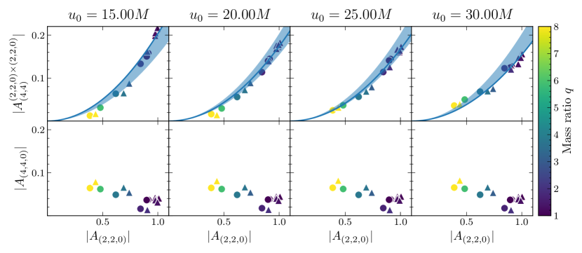
We show the main result of the fits in Fig. 1 for a range of initial times $u_{0}$ with which we find the best-fit amplitudes to be stable (shown later). In the top panel, we see that $A_{(2,2,0)}$ and $A_{(4,4)}^{(2,2,0)\times(2,2,0)}$ are consistent with a quadratic relationship, illustrated by the shaded blue region that is obtained by combining the fitted quadratic curves for $u_{0}\in[15M,30M]$. In this region, we find the ratio $A_{(4,4)}^{(2,2,0)\times(2,2,0)}/(A_{(2,2,0)})^{2}$ to range between 0.20 and 0.15. Again we emphasize that here $A_{(2,2,0)}$ has the mixing coefficients factored out, while $A_{(4,4)}^{(2,2,0)\times(2,2,0)}$ contains whatever angular structure arises through nonlinear effects. There is no noticeable difference in the quadratic relationship followed by the $0.7$ and $0.5$ spin families of waveforms, compared to the variations that are observed in the best-fit $A^{(2,2,0)\times(2,2,0)}_{(4,4)}$ due to the choice of the model start time $u_{0}$.

We emphasize that this quadratic behavior is unique to the $A_{(4,4)}^{(2,2,0)\times(2,2,0)}$ mode, as can be seen in the bottom panel of Fig. 1, where we show the best-fit linear amplitude $A_{(4,4,0)}$ as a function of $A_{(2,2,0)}$. These two modes are not related quadratically (for more on their scaling with mass ratio, see [61]), which confirms the distinct physical origin of $A_{(4,4,0)}$ and $A^{(2,2,0)\times(2,2,0)}_{(4,4)}$. The best-fit amplitudes of $A_{(4,4,0)}$ and $A_{(2,2,0)}$ are nearly constant across these values of $u_{0}$, which is why the four bottom figures look the same. A key result of Fig. 1 is that $A^{(2,2,0)\times(2,2,0)}_{(4,4)}$ is comparable to or larger (by a factor of $\sim 4$ in cases with $q\approx 1$) than $A_{(4,4,0)}$ at the time of the peak. Given that the exponential decay rates of $A^{(2,2,0)\times(2,2,0)}_{(4,4)}$ and $A_{(4,4,0)}$ for a BH with $\chi_{f}=0.7$ are $\text{Im}[M\omega_{(2,2,0)\times(2,2,0)}]=-0.16$ and $\text{Im}[M\omega_{(4,4,0)}]=-0.08$, respectively, even beyond $10M$ after $u_{\text{peak}}$ the quadratic mode will be larger than the linear mode for equal mass ratio binaries. Thus, for large SNR events in which the $(4,4)$ mode is detectable, the quadratic QNM could be measurable.

Comparisons.—Figure 2 shows the GW150914 simulation (SXS:BBH:0305) and its fitting at $u_{0}=20M$, the time at which the residual in the $(4,4)$ mode reaches its minimum. The top panel shows the waveform fit with the $(4,4)$ quadratic model $h^{\text{model},\,Q}_{(4,4)}$ as a function of time, where we find that it can fit rather well the amplitude and phase evolution of the numerical waveform at late times. The bottom panel shows the residual of the NR waveform with the linear and quadratic $(4,4)$ QNM models, $h^{\text{model},\,L}_{(4,4,2)}$ and $h^{\text{model},\,Q}_{(4,4)}$, and a conservative estimate for the numerical error obtained by comparing the highest and second highest resolution simulations for SXS:BBH:0305.

Figure 2: Top: in black, the NR waveform for the SXS:BBH:0305 simulation and its comparison to the quadratic $(4,4)$ QNM model with start time $u_{0}=20M$ (total is dashed blue; yellow and green are contributions from individual QNMs, respectively the linear $(4,4,1)$ and the quadratic $(2,2,0)\times(2,2,0)$). Bottom: residual in the $(4,4)$ mode when using the linear (solid red) or the quadratic (dashed blue) $(4,4)$ model. We also show a conservative estimate of the numerical error.

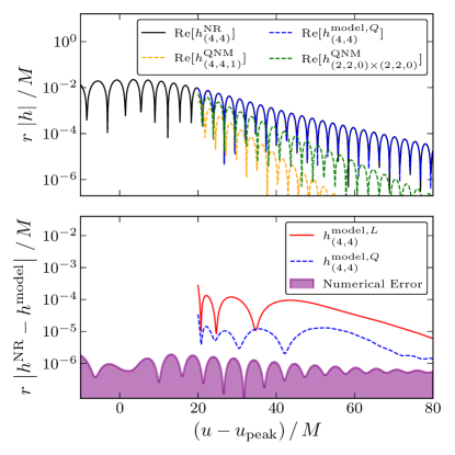
We see that even though the linear and quadratic $(4,4)$ models have the same number of free parameters, the residual of $h^{\text{model},\,Q}_{(4,4)}$ is nearly an order of magnitude better, which confirms the importance of including quadratic QNMs. Since, in general, the quadratic mode decays in time slower than the $(4,4,2)$ QNM, the quadratic model generally better describes the late time behavior of the waveform. In addition, the best-fit value of $A_{(4,4,0)}$—which is the most important QNM in the $(4,4)$ mode at late times—differs in the linear and quadratic models, which causes the residuals to be rather different even beyond $u=50M$ when we expect the overtones and quadratic mode to be subdominant.

Figure 3: Top: mismatch in the $(4,4)$ mode for SXS:BBH:0305, as well as for every other simulation examined, and a comparison to the numerical error floor. Bottom: amplitudes of the three QNM terms in the quadratic $(4,4)$ QNM model as a function of the model start time $u_{0}$.

In addition to the residuals, we quantify the goodness of fit by our models through the mismatch

$$\mathcal{M}=1-\text{Re}\left[\frac{\langle h_{(\ell,m)}^{\text{NR}}|h_{(\ell,m)}^{\text{model}}\rangle}{\sqrt{\langle h_{(\ell,m)}^{\text{NR}}|h_{(\ell,m)}^{\text{NR}}\rangle\langle h_{(\ell,m)}^{\text{model}}|h_{(\ell,m)}^{\text{model}}\rangle}}\right].$$ (8)

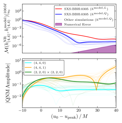
The top panel of Fig. 3 shows the mismatch in the $(4,4)$ mode between the NR waveform and the QNM model as a function of $u_{0}$. The red and blue lines show the results for the SXS:BBH:0305 simulation when the $(4,4)$ mode was modeled with $h^{\text{model},\,L}_{(4,4,2)}$ and $h^{\text{model},\,Q}_{(4,4)}$, respectively. As a reference, we also show the numerical error calculated for SXS:BBH:0305. We see that the numerical error is below the fitted model mismatches for $u_{0}\lesssim 40M$, but will cause the mismatch to worsen at later times. We also see that the linear model performs worse than the quadratic model for any $u_{0}$, confirming that the residual difference shown in the bottom panel of Fig. 2 was not a coincidence of the particular fitting time chosen there. At times $u_{0}\approx 20M$, we see that the mismatch is about 2 orders of magnitude better in the quadratic model. We find similar results for all of the simulations analyzed in this Letter (light blue thin curves show the mismatch of the $h^{\text{model},\,Q}_{(4,4)}$ in those simulations), although the mismatch difference becomes more modest for simulations with $q\approx 8$ since the relative amplitude of the quadratic mode decreases (cf. bottom panel of Fig. 1 where we see that amplitude of the $(2,2,0)$ mode decreases with $q$, while the amplitude of the $(4,4,0)$ mode increases with $q$). When comparing the mismatches to the error, we find that every simulation remains above the numerical error floor until $u_{0}\gtrsim 40M$.

In the bottom panel of Fig. 3, we show the best-fit amplitudes of the QNMs in the $(4,4)$ mode as functions of $u_{0}$. We show the results for SXS:BBH:0305 (thick lines) as well as the rest of the simulations (thin lines). We see that at $u_{0}\gtrsim 10M$ the amplitude of $A_{(4,4,0)}$ is extremely stable, but the faster the additional QNM decays, the more variations that are seen. Nevertheless, the $A^{(2,2,0)\times(2,2,0)}_{(4,4)}$ exhibits only $\sim 20\%$ variations for $u_{0}\in[15M,30M]$, whereas $A_{(4,4,1)}$ varies by $\sim 90\%$ in the same range. Before and near $u_{0}\approx 10M$ every amplitude shows considerable variations, which is why we use $u_{0}\geq 15M$ in this Letter. This suggests a need to improve the QNM model, either by including more overtones as in [10], modifying the time dependence of the linear [62] and quadratic terms, or considering more nonlinear effects.

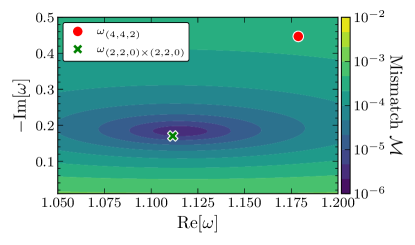
Finally we check which frequency is preferred by the $(4,4)$ mode of the numerical strain. For this, we fix two frequencies to be the linear $\omega_{(4,4,0)}$ and $\omega_{(4,4,1)}$ frequencies, and keep one frequency free. We vary the frequency of that third term and fit every amplitude to minimize the residual in Eq. (6). Figure 4 shows contours of the mismatch over the real and imaginary parts of the unknown frequency for the SXS:BBH:0305 simulation using $u_{0}=20M$. We confirm that the data clearly prefers the frequency $\omega_{(2,2,0)\times(2,2,0)}=2\omega_{(2,2,0)}$ over $\omega_{(4,4,2)}$.

Figure 4: Contour plot of the mismatch between the SXS:BBH:0305 waveform and a $(4,4)$ model with three QNMs, in which two frequencies are fixed to the GR predictions of the linear $(4,4,0)$ and $(4,4,1)$ QNMs, but the third is varied. The contour lines are logarithmically spaced in $\mathcal{M}$ between $10^{-6}$ and $10^{-2}$. The start time of the model is taken to be $u_{0}=20M$.

Conclusions.—We have shown that second-order effects are present in the ringdown phase of binary BH mergers for a wide range of mass ratios, matching theoretical expectations and helping improve ringdown modeling at late times. We analyzed 17 NR simulations and in every one of them we found that, in the $(\ell,m)=(4,4)$ mode, the quadratic QNM analyzed has a peak amplitude that is comparable to or larger than the $(\ell,m,n)=(4,4,0)$ fundamental linear QNM. Because of the relatively slow decay of this quadratic QNM, we find that for nearly equal-mass systems this QNM will be larger than the corresponding linear fundamental mode even $10M$ after $u_{\text{peak}}$.

These results highlight that we may be able to observe this nonlinear effect in future high-SNR GW events with a detectable $(4,4)$ harmonic. A quantitative analysis, and a generalization to other harmonics, will be performed in the future to assess in detail the detectability of quadratic QNMs and how well they can be distinguished from linear QNMs, for current GW detectors at design sensitivity as well as next-generation GW detectors. It would also be interesting to study how the linear/quadratic relationship of these nonlinearities varies with the spin of the remnant, especially as one approaches maximal spin.

The confirmation of quadratic QNMs opens new possibilities for more general understanding of the role of nonlinearities in the ringdown of perturbed black holes. It is now clear that we can readily improve the basic linear models that have been used previously in theoretical and observational ringdown analyses. Quadratic QNMs provide new opportunities to maximize the science return of GW detections, by increasing the likelihood of detecting multiple QNM frequencies. One of these key science goals is performing high-precision consistency tests of GR with GW observations. Fulfilling this aim will require a correct ringdown model, which incorporates the nonlinear effects that we have shown to be robustly present.

Acknowledgments.—We thank Max Isi and the Flatiron Institute for fostering discourse, and Vishal Baibhav, Emanuele Berti, Mark Cheung, Matt Giesler, Scott Hughes, and Max Isi for valuable conversations. Computations for this work were performed with the Wheeler cluster at Caltech. This work was supported in part by the Sherman Fairchild Foundation and by NSF Grants No. PHY-2011961, No. PHY-2011968, and No. OAC-1931266 at Caltech, as well as NSF Grants No. PHY-1912081, No. PHY-2207342, and No. OAC-1931280 at Cornell. The work of L.C.S. was partially supported by NSF CAREER Grant No. PHY-2047382. M.L. was funded by the Innovative Theoretical Cosmology Fellowship at Columbia University. L.H. was funded by the DOE DE-SC0011941 and a Simons Fellowship in Theoretical Physics. M.L. and L.C.S. thank the Benasque Science Center and the organizers of the 2022 workshop “New frontiers in strong gravity,” where some of this work was performed; and M.L. acknowledges NSF Grant No. PHY-1759835 for supporting travel to this workshop.

Note added.–Recently, we learned that Cheung et al. conducted a similar study, whose results are consistent with ours [63].

References

- Stephani et al. [2003] H. Stephani, D. Kramer, M. A. H. MacCallum, C. Hoenselaers, and E. Herlt, Exact solutions of Einstein’s field equations, Cambridge Monographs on Mathematical Physics (Cambridge Univ. Press, Cambridge, 2003).
- Griffiths and Podolsky [2009] J. B. Griffiths and J. Podolsky, Exact Space-Times in Einstein’s General Relativity, Cambridge Monographs on Mathematical Physics (Cambridge University Press, Cambridge, 2009).
- Regge and Wheeler [1957] T. Regge and J. A. Wheeler, Stability of a Schwarzschild singularity, Phys. Rev. 108, 1063 (1957).
- Zerilli [1970] F. J. Zerilli, Gravitational field of a particle falling in a schwarzschild geometry analyzed in tensor harmonics, Phys. Rev. D 2, 2141 (1970).
- Teukolsky [1973] S. A. Teukolsky, Perturbations of a rotating black hole. 1. Fundamental equations for gravitational electromagnetic and neutrino field perturbations, Astrophys. J. 185, 635 (1973).
- Penrose [1969] R. Penrose, Gravitational collapse: The role of general relativity, Riv. Nuovo Cim. 1, 252 (1969).
- Chrusciel et al. [2012] P. T. Chrusciel, J. Lopes Costa, and M. Heusler, Stationary Black Holes: Uniqueness and Beyond, Living Rev. Rel. 15, 7 (2012), arXiv:1205.6112 [gr-qc] .
- Blanchet [2014] L. Blanchet, Gravitational Radiation from Post-Newtonian Sources and Inspiralling Compact Binaries, Living Rev. Rel. 17, 2 (2014), arXiv:1310.1528 [gr-qc] .
- Berti et al. [2009] E. Berti, V. Cardoso, and A. O. Starinets, Quasinormal modes of black holes and black branes, Class. Quant. Grav. 26, 163001 (2009), arXiv:0905.2975 [gr-qc] .
- Giesler et al. [2019] M. Giesler, M. Isi, M. A. Scheel, and S. Teukolsky, Black Hole Ringdown: The Importance of Overtones, Phys. Rev. X 9, 041060 (2019), arXiv:1903.08284 [gr-qc] .
- Bhagwat et al. [2020] S. Bhagwat, X. J. Forteza, P. Pani, and V. Ferrari, Ringdown overtones, black hole spectroscopy, and no-hair theorem tests, Phys. Rev. D 101, 044033 (2020), arXiv:1910.08708 [gr-qc] .
- Cook [2020] G. B. Cook, Aspects of multimode Kerr ringdown fitting, Phys. Rev. D 102, 024027 (2020), arXiv:2004.08347 [gr-qc] .
- Jiménez Forteza et al. [2020] X. Jiménez Forteza, S. Bhagwat, P. Pani, and V. Ferrari, Spectroscopy of binary black hole ringdown using overtones and angular modes, Phys. Rev. D 102, 044053 (2020), arXiv:2005.03260 [gr-qc] .
- Dhani [2021] A. Dhani, Importance of mirror modes in binary black hole ringdown waveform, Phys. Rev. D 103, 104048 (2021), arXiv:2010.08602 [gr-qc] .
- Finch and Moore [2022] E. Finch and C. J. Moore, Searching for a Ringdown Overtone in GW150914, arXiv:2205.07809 [gr-qc] .
- Teukolsky [2015] S. A. Teukolsky, The Kerr Metric, Class. Quant. Grav. 32, 124006 (2015), arXiv:1410.2130 [gr-qc] .
- Magaña Zertuche et al. [2022] L. Magaña Zertuche, K. Mitman, N. Khera, L. C. Stein, M. Boyle, N. Deppe, F. Hébert, D. A. B. Iozzo, L. E. Kidder, J. Moxon, H. P. Pfeiffer, M. A. Scheel, S. A. Teukolsky, W. Throwe, and N. Vu, High precision ringdown modeling: Multimode fits and BMS frames, Physical Review D 105, 10.1103/physrevd.105.104015 (2022), 2110.15922 .
- Leaver [1986] E. W. Leaver, Spectral decomposition of the perturbation response of the Schwarzschild geometry, Phys. Rev. D 34, 384 (1986).
- Isi et al. [2019] M. Isi, M. Giesler, W. M. Farr, M. A. Scheel, and S. A. Teukolsky, Testing the no-hair theorem with GW150914, Phys. Rev. Lett. 123, 111102 (2019), arXiv:1905.00869 [gr-qc] .
- Cotesta et al. [2022] R. Cotesta, G. Carullo, E. Berti, and V. Cardoso, On the detection of ringdown overtones in GW150914, arXiv:2201.00822 [gr-qc] .
- Isi and Farr [2022] M. Isi and W. M. Farr, Revisiting the ringdown of GW150914, arXiv:2202.02941 [gr-qc] .
- Berti et al. [2016] E. Berti, A. Sesana, E. Barausse, V. Cardoso, and K. Belczynski, Spectroscopy of Kerr black holes with Earth- and space-based interferometers, Phys. Rev. Lett. 117, 101102 (2016), arXiv:1605.09286 [gr-qc] .
- Ota and Chirenti [2020] I. Ota and C. Chirenti, Overtones or higher harmonics? Prospects for testing the no-hair theorem with gravitational wave detections, Phys. Rev. D 101, 104005 (2020), arXiv:1911.00440 [gr-qc] .
- Bhagwat et al. [2022] S. Bhagwat, C. Pacilio, E. Barausse, and P. Pani, Landscape of massive black-hole spectroscopy with LISA and the Einstein Telescope, Phys. Rev. D 105, 124063 (2022), arXiv:2201.00023 [gr-qc] .
- Berti et al. [2018] E. Berti, K. Yagi, H. Yang, and N. Yunes, Extreme gravity tests with gravitational waves from compact binary coalescences: (II) ringdown, General Relativity and Gravitation 50, 10.1007/s10714-018-2372-6 (2018), 1801.03587 .
- Abbott et al. [2021] R. Abbott et al. (LIGO Scientific, VIRGO, KAGRA), Tests of General Relativity with GWTC-3, arXiv:2112.06861 [gr-qc] .
- Abbott et al. [2018] B. P. Abbott et al. (KAGRA, LIGO Scientific, Virgo, VIRGO), Prospects for observing and localizing gravitational-wave transients with Advanced LIGO, Advanced Virgo and KAGRA, Living Rev. Rel. 21, 3 (2018), arXiv:1304.0670 [gr-qc] .
- Team [2018] L. S. Team, LISA Science Requirement Document.
- Maggiore et al. [2020] M. Maggiore et al., Science Case for the Einstein Telescope, JCAP 03, 050, arXiv:1912.02622 [astro-ph.CO] .
- Evans et al. [2021] M. Evans et al., A Horizon Study for Cosmic Explorer: Science, Observatories, and Community, arXiv:2109.09882 [astro-ph.IM] .
- London et al. [2014] L. London, D. Shoemaker, and J. Healy, Modeling ringdown: Beyond the fundamental quasinormal modes, Phys. Rev. D 90, 124032 (2014), [Erratum: Phys.Rev.D 94, 069902 (2016)], arXiv:1404.3197 [gr-qc] .
- Ma et al. [2022] S. Ma, K. Mitman, L. Sun, N. Deppe, F. Hébert, L. E. Kidder, J. Moxon, W. Throwe, N. L. Vu, and Y. Chen, Collective filters: a new approach to analyze the gravitational-wave ringdown of binary black-hole mergers, arXiv:2207.10870 [gr-qc] .
- Gleiser et al. [1996a] R. J. Gleiser, C. O. Nicasio, R. H. Price, and J. Pullin, Colliding black holes: How far can the close approximation go?, Phys. Rev. Lett. 77, 4483 (1996a), arXiv:gr-qc/9609022 .
- Gleiser et al. [1996b] R. J. Gleiser, C. O. Nicasio, R. H. Price, and J. Pullin, Second order perturbations of a Schwarzschild black hole, Class. Quant. Grav. 13, L117 (1996b), arXiv:gr-qc/9510049 .
- Gleiser et al. [2000] R. J. Gleiser, C. O. Nicasio, R. H. Price, and J. Pullin, Gravitational radiation from Schwarzschild black holes: The Second order perturbation formalism, Phys. Rept. 325, 41 (2000), arXiv:gr-qc/9807077 .
- Ioka and Nakano [2007] K. Ioka and H. Nakano, Second and higher-order quasi-normal modes in binary black hole mergers, Phys. Rev. D 76, 061503 (2007), arXiv:0704.3467 [astro-ph] .
- Nakano and Ioka [2007] H. Nakano and K. Ioka, Second Order Quasi-Normal Mode of the Schwarzschild Black Hole, Phys. Rev. D 76, 084007 (2007), arXiv:0708.0450 [gr-qc] .
- Okuzumi et al. [2008] S. Okuzumi, K. Ioka, and M.-a. Sakagami, Possible Discovery of Nonlinear Tail and Quasinormal Modes in Black Hole Ringdown, Phys. Rev. D 77, 124018 (2008), arXiv:0803.0501 [gr-qc] .
- Brizuela et al. [2009] D. Brizuela, J. M. Martin-Garcia, and M. Tiglio, A Complete gauge-invariant formalism for arbitrary second-order perturbations of a Schwarzschild black hole, Phys. Rev. D 80, 024021 (2009), arXiv:0903.1134 [gr-qc] .
- Pazos et al. [2010] E. Pazos, D. Brizuela, J. M. Martin-Garcia, and M. Tiglio, Mode coupling of Schwarzschild perturbations: Ringdown frequencies, Phys. Rev. D 82, 104028 (2010), arXiv:1009.4665 [gr-qc] .
- Ripley et al. [2021] J. L. Ripley, N. Loutrel, E. Giorgi, and F. Pretorius, Numerical computation of second order vacuum perturbations of Kerr black holes, Phys. Rev. D 103, 104018 (2021), arXiv:2010.00162 [gr-qc] .
- Loutrel et al. [2021] N. Loutrel, J. L. Ripley, E. Giorgi, and F. Pretorius, Second Order Perturbations of Kerr Black Holes: Reconstruction of the Metric, Phys. Rev. D 103, 104017 (2021), arXiv:2008.11770 [gr-qc] .
- Lagos and Hui [2022] M. Lagos and L. Hui, Generation and propagation of nonlinear quasi-normal modes of a Schwarzschild black hole, arXiv:2208.07379 [gr-qc] .
- Campanelli and Lousto [1999] M. Campanelli and C. O. Lousto, Second order gauge invariant gravitational perturbations of a Kerr black hole, Phys. Rev. D 59, 124022 (1999), arXiv:gr-qc/9811019 .
- Mitman et al. [2020] K. Mitman, J. Moxon, M. A. Scheel, S. A. Teukolsky, M. Boyle, N. Deppe, L. E. Kidder, and W. Throwe, Computation of displacement and spin gravitational memory in numerical relativity, Phys. Rev. D 102, 104007 (2020), arXiv:2007.11562 [gr-qc] .
- Boyle et al. [2019] M. Boyle et al., The SXS Collaboration catalog of binary black hole simulations, Class. Quant. Grav. 36, 195006 (2019), arXiv:1904.04831 [gr-qc] .
- Abbott et al. [2016] B. P. Abbott et al. (LIGO Scientific, Virgo), GW150914: First results from the search for binary black hole coalescence with Advanced LIGO, Phys. Rev. D 93, 122003 (2016), arXiv:1602.03839 [gr-qc] .
- [48] https://www.black-holes.org/code/SpEC.html.
- [49] SXS Gravitational Waveform Database, http://www.black-holes.org/waveforms.
- Moxon et al. [2020] J. Moxon, M. A. Scheel, and S. A. Teukolsky, Improved Cauchy-characteristic evolution system for high-precision numerical relativity waveforms, Phys. Rev. D 102, 044052 (2020), arXiv:2007.01339 [gr-qc] .
- Moxon et al. [2021] J. Moxon, M. A. Scheel, S. A. Teukolsky, N. Deppe, N. Fischer, F. Hébert, L. E. Kidder, and W. Throwe, The SpECTRE Cauchy-characteristic evolution system for rapid, precise waveform extraction, arXiv:2110.08635 [gr-qc] .
- Deppe et al. [2020] N. Deppe, W. Throwe, L. E. Kidder, N. L. Fischer, C. Armaza, G. S. Bonilla, F. Hébert, P. Kumar, G. Lovelace, J. Moxon, E. O’Shea, H. P. Pfeiffer, M. A. Scheel, S. A. Teukolsky, I. Anantpurkar, M. Boyle, F. Foucart, M. Giesler, D. A. B. Iozzo, I. Legred, D. Li, A. Macedo, D. Melchor, M. Morales, T. Ramirez, H. R. Rüter, J. Sanchez, S. Thomas, and T. Wlodarczyk, SpECTRE (2020).
- Mitman et al. [2021] K. Mitman et al., Fixing the BMS frame of numerical relativity waveforms, Phys. Rev. D 104, 024051 (2021), arXiv:2105.02300 [gr-qc] .
- Mitman et al. [2022] K. Mitman et al., Fixing the BMS Frame of Numerical Relativity Waveforms with BMS Charges, arXiv:2208.04356 [gr-qc] .
- Boyle et al. [2020] M. Boyle, D. Iozzo, and L. C. Stein, moble/scri: v1.2 (2020).
- Boyle [2013] M. Boyle, Angular velocity of gravitational radiation from precessing binaries and the corotating frame, Phys. Rev. D 87, 104006 (2013), arXiv:1302.2919 [gr-qc] .
- Boyle et al. [2014] M. Boyle, L. E. Kidder, S. Ossokine, and H. P. Pfeiffer, Gravitational-wave modes from precessing black-hole binaries, arXiv:1409.4431 [gr-qc] .
- Boyle [2016] M. Boyle, Transformations of asymptotic gravitational-wave data, Phys. Rev. D 93, 084031 (2016), arXiv:1509.00862 [gr-qc] .
- Virtanen et al. [2020] P. Virtanen, R. Gommers, T. E. Oliphant, M. Haberland, T. Reddy, D. Cournapeau, E. Burovski, P. Peterson, W. Weckesser, J. Bright, S. J. van der Walt, M. Brett, J. Wilson, K. J. Millman, N. Mayorov, A. R. J. Nelson, E. Jones, R. Kern, E. Larson, C. J. Carey, İ. Polat, Y. Feng, E. W. Moore, J. VanderPlas, D. Laxalde, J. Perktold, R. Cimrman, I. Henriksen, E. A. Quintero, C. R. Harris, A. M. Archibald, A. H. Ribeiro, F. Pedregosa, P. van Mulbregt, and SciPy 1.0 Contributors, SciPy 1.0: Fundamental Algorithms for Scientific Computing in Python, Nature Methods 17, 261 (2020).
- Stein [2019] L. C. Stein, qnm: A Python package for calculating Kerr quasinormal modes, separation constants, and spherical-spheroidal mixing coefficients, J. Open Source Softw. 4, 1683 (2019), arXiv:1908.10377 [gr-qc] .
- Borhanian et al. [2020] S. Borhanian, K. G. Arun, H. P. Pfeiffer, and B. S. Sathyaprakash, Comparison of post-Newtonian mode amplitudes with numerical relativity simulations of binary black holes, Class. Quant. Grav. 37, 065006 (2020), arXiv:1901.08516 [gr-qc] .
- Sberna et al. [2022] L. Sberna, P. Bosch, W. E. East, S. R. Green, and L. Lehner, Nonlinear effects in the black hole ringdown: Absorption-induced mode excitation, Phys. Rev. D 105, 064046 (2022), arXiv:2112.11168 [gr-qc] .
- Cheung et al. [2022] M. H.-Y. Cheung, V. Baibhav, E. Berti, V. Cardoso, G. Carullo, R. Cotesta, W. Del Pozzo, F. Duque, T. Helfer, E. Shukla, and K. W. K. Wong, Nonlinear effects in black hole ringdown, arXiv:2208.07374 [gr-qc] .