Exploring the Neutrino Sector of the Minimal Left-Right Symmetric Model

Abstract

We explore the neutrino sector of the minimal left-right symmetric model, with the additional charge conjugation discrete symmetry, in the tuned regime where type-I and type-II seesaw mechanisms are equally responsible for the light neutrino masses. We show that unless the charged lepton mixing matrix is the identity and the right handed neutrino mass matrix has no phases, we expect sizable lepton flavor violation and electron dipole moment in this region. We use results from recent neutrino oscillation fits, bounds on neutrinoless double beta decay, $\mu\to e\gamma$, $\mu\to 3e$, $\mu\to e$ conversion in nuclei, the muon anomalous magnetic moment, the electron electric dipole moment and cosmology to determine the viability of this region. We derive stringent limits on the heavy neutrino masses and mixing angles as well as on the vacuum expectation value $v_{L}$, which drives the type-II seesaw contribution, using the current data. We discuss the perspectives of probing the remaining parameter space by future experiments.

1 Introduction

The neutrinos we know are massive and light. Data on neutrino flavor oscillations by a variety of different solar, atmospheric, reactor and accelerator neutrino experiments need two different mass squared difference scales $\Delta m^{2}_{21}\approx 7.5\times 10^{-5}$ eV² and $|\Delta m^{2}_{31,32}|\approx 2.5\times 10^{-3}$ eV² to be explained Esteban:2020cvm . These measurements give rise to two possible mass ordering: $m_{1}<m_{2}<m_{3}$ (normal) or $m_{3}<m_{1}<m_{2}$ (inverted). Although it may seem that there is a slight data preference for normal ordering (NO), inverted ordering (IO) cannot be discarded Kelly:2020fkv . Complementary information comes from the KATRIN (KArlsruhe TRItium Neutrino) experiment that recently updated their limit on the effective electon neutrino mass to $m_{\beta}<0.8$ eV at 90% CL KATRIN:2021uub . Moreover, we need three light neutrinos to explain cosmological observations that constrain the effective number of relativistic degrees of freedom to $N_{\rm eff}=2.99\pm 0.17$ and the sum of neutrino masses $\sum m_{\nu}<0.12$ eV at 95% CL Planck:2018vyg .

In spite of the fact that the theoretical origin of neutrino masses is unknown, the current very successful standard paradigm indicates that neutrino mass eigenstates are a particular admixture of the Standard Model (SM) neutrino flavor eigenstates. So neutrino oscillations present today the only solid experimental evidences of Lepton Flavor Violating (LFV) processes in nature.

An unprecedented experimental campaign to probe rare LFV processes with charged leptons is about to start. Experiments using a $\mu$ beam such as MEG II MEGII:2018kmf , Mu3e Blondel:2013ia ; Berger:2014vba , COMET COMET:2018auw and Mu2e Mu2e:2014fns are prone to collect datasets of about $10^{15}-10^{17}$ muons, increasing the sensitivity to LFV transitions such as $\mu\to e\gamma$, $\mu\to 3e$ and $\mu N\to eN$ by more than an order of magnitude down from current bounds.

However, although the leptonic charge associated to each lepton generation $L_{\alpha}\,(\alpha=e,\mu,\tau)$ is not conserved, oscillations do not allow us to say anything about the conservation of the total leptonic charge $L=L_{e}+L_{\mu}+L_{\tau}$. For this we need to seach for Lepton Number Violating processes (LNV). Neutrinos can be Dirac or Majorana fermions. In the first case, neutrino interactions (including mass terms) must conserve $L$, in the second, neutrino interactions (including mass terms) do not conserve $L$. So the neutrino nature and $L$-conservation are interconnected.

Majorana neutrinos can manifest themselves in $|\Delta L|=2$ transitions of which the neutrinoless double-beta decay ($0\nu\beta\beta$) is the most promising possibility. That is why there is a robust experimental program devoted to search for this decay using a variety of isotopes (⁷⁶ Ge,⁸²Se,¹³⁰Te and ¹³⁶Xe), with detector masses in the range 100 kg – 10000 kg, using different techniques, aiming to reach sensitivies on the effective Majorana neutrino mass $m_{\beta\beta}\lesssim$ few meV Agostini:2017jim .

In the SM $L$-conservation is due to an accidental global $U(1)_{L}$ symmetry, which we expect to be broken by quantum fluctuations. The smallness of neutrino masses may be understood in a plausible way in extensions of the SM by the introduction of new fields that are integrated out at low energies generating the so-called Weinberg Weinberg:1979sa operator. This operator leads to a Majorana mass term and encapsulates the so-called seesaw mechanisms Minkowski:1977sc ; Gell-Mann:1979vob ; Yanagida:1979as ; Mohapatra:1979ia ; Schechter:1980gr ; Foot:1988aq . This mechanism emerges inherently in theories where right-handed neutrinos are a necessity such as left-right symmetric models. Although these models were initially motivated by a desired to understand the origin of parity violation in weak interactions, they turned out to be a natural framework to explain the pattern of neutrino masses.

In the Minimal Left-Right Symmetric Model (MLRSM) Pati:1974yy ; Mohapatra:1974gc ; Senjanovic:1975rk ; Mohapatra:1979ia ; Mohapatra:1980yp , after left-right and electroweak symmetry breaking, the light neutrino mass term ($m_{\nu}$) is generated from the type-I and type-II seesaw mechanisms

$$m_{\nu} = m_{{\rm I}}+m_{{\rm II}},$$ (1)

where schematically, $m_{{\rm I}}\sim v^{2}/v_{R}$ and $m_{{\rm II}}\sim v_{L}$ with $v=246$ GeV the effective Higgs vacuum expectation value (vev), and $v_{L}\ll v_{R}$ are the vevs associated with left and right triplet Higgs which spontaneously break the left-right symmetry. Depending on the ratio $v_{L}/v_{R}$, one can have three scenarios: (i) a type-I dominated scenario when $m_{{\rm I}}\gg m_{{\rm II}}$, (ii) a type-II dominated scenario when $m_{{\rm I}}\ll m_{{\rm II}}$, or (iii) a tuned scenario when $m_{{\rm I}}\simeq m_{{\rm II}}$. The mixing between the SM neutrinos and (mostly right-handed) heavy neutrinos (in the following we will denote this the active-sterile mixing) is proportional to $\sqrt{m_{{\rm I}}/v_{R}}$ and hence in the tuned scenario, if $m_{{\rm I}}\simeq m_{{\rm II}}\gg m_{\nu}$, one can have a sufficiently large active-sterile mixing that leads to signatures in present and forthcoming experiments. In contrast to previous works that assumed either type I Barry:2013xxa ; BhupalDev:2014qbx ; Bambhaniya:2015ipg ; Goswami:2020loc or type II Tello:2010am ; Barry:2013xxa ; Bambhaniya:2015ipg ; Li:2020flq seesaw dominance, although we also discuss type-I seesaw here, we are mainly interested in exploring the tuned scenario where both types of seesaw are comparable. This could have interesting experimental signatures due to active-sterile mixing and, as we shall show, allows us to study the role played by the different sectors of the MLRSM in various new physics processes implicating the leptonic sector.

This work is organized as follows. In section 2 we introduce the leptonic sector of the MLRSM, which is the focus of our work. We examine the physical parameters of this sector in the general case and for a discrete left-right symmetry realised by charge conjugation or parity. We describe how to reconstruct the neutrino mass in each of these cases. We will then assume the charge conjugation symmetry. In section 3 we describe the two regimes of our study (type I and tuned), the relevant parameters of the model used in the phenomenological analysis and present a standard and three other benchmark cases. We discuss the model contributions to several observables in the neutrino sector, $0\nu\beta\beta$, LFV processes, the anomalous magnetic moment of the muon ($a_{\mu}$) and the electric dipole moment ($d_{\ell}$) and their dependence on the lightest heavy neutrinos mass ($m_{4}$) in view of current and future experimental bounds. We also comment on the impact of the model in the new CDF II result on the W boson mass. In section 4 we combine all available limits on the studied observables to determine the current allowed region for the heavy neutrino sector parameters. We also consider the effect of changing the standard benchmark value of the most significant parameters on this allowed region. We comment on the range of the heavy neutrino sector parameters that can be explored by future experiments and discuss some correlations among observables. Finally, in section 5 we draw our conclusions. In appendix A we describe for completeness the other sectors of the MLRSM, in appendix B we give approximate expressions for the form factors needed for the LFV, $a_{\mu}$ and $d_{\ell}$ calculations and in appendix C we show some supplementary plots to illustrate the small dependence of our results on parameters otherwise fixed in our study.

2 On the Leptonic Sector of the Minimal Left-Right Symmetric Model

The MLRSM is a gauge theory that, while keeping the fermionic content of the SM basically untouched (except for the neutrino sector as right-handed neutrinos are included), doubles its gauge sector by extending the gauge group to $SU(2)_{L}\times SU(2)_{R}\times U(1)_{B-L}$, possibly supplemented by a discrete symmetry between the left and right sectors. Here we will discuss the pattern of the mass matrices in the leptonic sector of the MLRSM. A description of the other sectors of the model relevant to our work can be found in Appendix A.

The mass matrices in the leptonic sector of the MLRSM depends on the symmetries imposed at high energies. To understand that, let us examine the Yukawa interactions in the leptonic sector given by

$${\cal L}_{\ell} = -\overline{L_{L}}\left(h_{l}\mathbf{\Phi}+\tilde{h}_{l}\tilde{\mathbf{\Phi}}\right)L_{R}-\overline{L_{L}^{c}}i\sigma_{2}\mathbf{\Delta}_{L}h_{M}L_{L}-\overline{L_{R}^{c}}i\sigma_{2}\mathbf{\Delta}_{R}\tilde{h}_{M}L_{R}+{\rm h.c.},$$ (2)

where $L_{L}\sim\left(2,1,-1\right)$, $L_{R}\sim\left(1,2,-1\right)$ are the left- and right-handed leptons and the scalars are $\mathbf{\Phi}\sim\left(2,2,0\right)$ with $\tilde{\mathbf{\Phi}}\equiv i\sigma_{2}\mathbf{\Phi^{*}}\sigma_{2}$, $\mathbf{\Delta}_{L}\sim\left(3,1,2\right)$ and $\mathbf{\Delta}_{R}\sim\left(1,3,2\right)$, in parentheses we show their quantum numbers with respect to the model gauge symmetry groups. In the above, we have left the flavor indices which run from 1 to 3 of $L_{L}$ and $L_{R}$ implicit and in the flavor space, both $h_{l}$ and $\tilde{h}_{l}$ are general $3\times 3$ complex matrices while $h_{M}$ and $\tilde{h}_{M}$ are general $3\times 3$ complex symmetric matrices. Let us count the physical parameters for the following cases: general, charge conjugation (${\cal C}$) and parity (${\cal P})$ symmetry.

1. General case

   Without loss of generality, we can rotate both left-handed and right-handed lepton doublets to make both $h_{M}$ and $\tilde{h}_{M}$ real and diagonal. Let us count the parameters in the Lagrangian, we have $9+9+3+3=24$ moduli and $9+9=18$ phases. The 24 moduli would correspond to 12 “low-energy” observables (3 charged lepton masses, 3 light neutrino masses, 3 heavy neutrino masses and 3 leptonic mixing angles) plus 12 additional “high-energy” parameters. The 18 phases would correspond to 3 leptonic CP phases $(\delta,\alpha_{1},\alpha_{2})$ plus 15 “high-energy” additional phases.

2. ${\cal C}$ symmetry

   Under ${\cal C}$ the fields in eq. (2) transform as

   $$L_{L}\leftrightarrow L_{R}^{c},\;\;\;\mathbf{\Delta}_{L}\leftrightarrow\mathbf{\Delta}_{R}^{\dagger},\;\;\;\mathbf{\Phi}\leftrightarrow\mathbf{\Phi}^{T}\,,$$ (3)

   so in this case, we have $h_{l}=h_{l}^{T}$, $\tilde{h}_{l}=\tilde{h}_{l}^{T}$ and $h_{M}=\tilde{h}_{M}^{*}$. We will rotate the lepton fields such that $h_{M}=\tilde{h}_{M}^{*}$ is diagonal but we will keep the three phases. The Lagrangian parameters are now $6+6+3=15$ moduli and $6+6=12$ phases. So under this extra symmetry there are only 3 additional “high-energy” parameters and 9 additional “high-energy” phases.

3. ${\cal P}$ symmetry

   Under ${\cal P}$ the fields in eq. (2) transform as

   $$L_{L}\leftrightarrow L_{R},\;\;\;\mathbf{\Delta}_{L}\leftrightarrow\mathbf{\Delta}_{R},\;\;\;\mathbf{\Phi}\leftrightarrow\mathbf{\Phi}^{\dagger}\,,$$ (4)

   so in this case, we have $h_{l}=h_{l}^{\dagger}$, $\tilde{h}_{l}=\tilde{h}_{l}^{\dagger}$ and $h_{M}=\tilde{h}_{M}$. We can again make $h_{M}$ real and diagonal. The Lagrangian parameters reduce to $6+6+3=15$ moduli and $3+3=6$ phases. The difference from the ${\cal C}$ case is that now we have only 3 additional “high-energy” phases instead of 9.

Assuming real vevs for the scalar fields, after the left-right and electroweak symmetry breaking the charged lepton mass matrix becomes

$$M_{l}=\frac{1}{\sqrt{2}}\left(h_{l}\,\kappa_{2}+\tilde{h}_{l}\,\kappa_{1}\right)\,,$$ (5)

where $\kappa_{1}$ and $\kappa_{2}$ are the vevs of $\mathbf{\Phi}$. Assuming $v_{R}^{2}\gg\kappa_{1}^{2}+\kappa_{2}^{2}\gg v_{L}^{2}$ where $v_{R}$ and $v_{L}$ are, respectively, the vevs of $\mathbf{\Delta}_{R}$ and $\mathbf{\Delta}_{L}$, we need

$$\kappa_{+}^{2}\equiv\kappa_{1}^{2}+\kappa_{2}^{2}=v^{2}=(246\,{\rm GeV})^{2}\,,$$ (6)

to reproduce the observed masses of the $Z$ and $W$ bosons. Two of the four vevs can be complex. In the view that there are already several new phases which are not constrained in the leptonic sector, the possibility of complex vevs will not be explored in this work.

Eq. (5) can be put in a diagonal form by a biunitary transformation

$$M_{l}=U_{L}^{\dagger}\hat{M_{l}}U_{R}\,,$$ (7)

where $\hat{M_{l}}={\text{diag}}(m_{e},m_{\mu},m_{\tau})$ and $U_{L}^{*}=U_{R}$ if $M_{l}$ is symmetric (for ${\cal C}$) or $U_{L}=U_{R}$ if $M_{l}$ is hermitian (for ${\cal P}$).

In the charged lepton mass basis, the $6\times 6$ neutral lepton mass matrix ${\cal M}_{\nu}$ defined by $\bar{\nu}{\cal M}_{\nu}\nu^{c}$ where $\nu=\left(\nu_{eL},\nu_{\mu L},\nu_{\tau L},\nu_{eR}^{\quad c},\nu_{\mu R}^{\quad c},\nu_{\tau R}^{\quad c}\right)^{T}$, is given by

$${\cal M}_{\nu}={\cal V}\,{\cal M}_{0}\,{\cal V}^{T}\,,$$ (8)

where ${\cal V}$ is the unitary matrix defined by

$${\cal V}\equiv\left(\begin{array}[]{cc}U_{L}&0\\ 0&U_{R}^{*}\end{array}\right)\,,$$ (9)

and ${\cal M}_{0}$ is the mass matrix defined by

$${\cal M}_{0}\equiv\left(\begin{array}[]{cc}M_{L}^{\dagger}&M_{D}\\ M_{D}^{T}&M_{R}\end{array}\right)\,,$$ (10)

with diagonal block matrices

$$M_{L} = \sqrt{2}\,h_{M}\,v_{L}\,,$$ (11)

$$M_{R} = \sqrt{2}\,\tilde{h}_{M}\,v_{R}\,,$$

and the Dirac neutrino mass matrix

$$M_{D}=\frac{1}{\sqrt{2}}\left(h_{l}\,\kappa_{1}+\tilde{h}_{l}\,\kappa_{2}\right)\,.$$ (12)

For ${\cal C}$ symmetry, $M_{L}=v_{L}M_{R}^{*}/v_{R}$ and $M_{D}$ is symmetric while for ${\cal P}$ symmetry, $M_{L}=v_{L}M_{R}/v_{R}$ and $M_{D}$ is hermitian.

We can block diagonalize ${\cal M}_{0}$ to obtain the $3\times 3$ light neutrino mass matrix. The leading term in the seesaw approximation $|M_{D}|\ll|M_{R}|$ is

$$m_{\nu}=m_{{\rm I}}+m_{{\rm II}}=-M_{D}M_{R}^{-1}M_{D}^{T}+M_{L}^{\dagger}=-\frac{1}{\sqrt{2}\,v_{R}}M_{D}{\tilde{h}_{M}}^{-1}M_{D}^{T}+\sqrt{2}\,h_{M}^{\dagger}\,v_{L}\,,$$ (13)

the first being the type-I and the second the type-II seesaw contributions, which in the charged lepton mass basis defines the the leptonic mixing matrix $U_{\rm PMNS}$ by

$$U_{L}\,m_{\nu}\,U_{L}^{T}\equiv U_{\rm PMNS}\,\hat{m}_{\nu}\,U^{T}_{\rm PMNS}\,,$$ (14)

with $\hat{m}_{\nu}={\text{diag}}(m_{1},m_{2},m_{3})$ the diagonal light neutrino mass matrix. So we can also write in this basis $m_{\nu}$ as

$$m_{\nu}=U_{L}^{\dagger}\,U_{\rm PMNS}\,\,\hat{m}_{\nu}\,U_{\rm PMNS}^{T}\,U_{L}^{*}\,.$$ (15)

The heavy neutrino mass matrix at the leading order is just $M_{R}=\sqrt{2}\tilde{h}_{M}v_{R}$. At the minimum of the scalar potential, the vevs $v_{R}$, $v_{L}$ and $\kappa_{+}$ satisfy the relation Deshpande:1990ip

$$v_{L}v_{R}=\gamma\kappa_{+}^{2},$$ (16)

where

$$\gamma=\frac{\beta_{1}\kappa_{1}\kappa_{2}+\beta_{2}\kappa_{1}^{2}+\beta_{3}\kappa_{2}^{2}}{(2\rho_{1}-\rho_{3})\kappa_{+}^{2}},$$ (17)

with $\beta_{i}$ and $\rho_{i}$ the relevant dimensionless couplings in the scalar potential. In the absence of tuning, $\gamma$ would be of the order of one. In this work, we are exploring sub-TeV scale right-handed neutrinos which implies $\gamma\ll 1$ or tuning of the parameters of the scalar potential Deshpande:1990ip .

2.1 Parametrization and Neutrino Mass Reconstruction

From eq. (13), we can write the type-I contribution as

$$m_{\rm I}=-M_{D}M_{R}^{-1}M_{D}^{T}=m_{\nu}-M_{L}^{\dagger}.$$ (18)

Multiplying by $M_{R}^{-1}$ from the right, we have

$$M_{D}M_{R}^{-1}M_{D}^{T}M_{R}^{-1}=M_{L}^{\dagger}M_{R}^{-1}-m_{\nu}M_{R}^{-1}.$$ (19)

Since the active-sterile mixing (that we will discuss more later) is proportional to $M_{D}M_{R}^{-1}$, it can be enhanced if $|M_{L}^{\dagger}|\gg|m_{\nu}|$ i.e. if we are in the tuned scenario where $m_{\rm I}\simeq m_{\rm II}$. Next, we discuss the solutions for $M_{D}$ in the three cases of interest.

1. General case

   There are sufficient degrees of freedom to construct a general complex Dirac matrix $M_{D}$ based on the Casas-Ibarra parametrization Casas:2001sr

   $$M_{D}=B^{\dagger}\sqrt{\hat{m}_{\rm I}}\,R\,\sqrt{M_{R}}\,,$$ (20)

   where $R$ is a complex orthogonal matrix and $B$ is a unitary matrix which diagonalizes $m_{\nu}-M_{L}^{\dagger}$

   $$m_{\rm I}=-B^{\dagger}\,\hat{m}_{\rm I}\,B^{*}=m_{\nu}-M_{L}^{\dagger}\,,$$ (21)

   with $\hat{m}_{\rm I}$ a diagonal matrix containing the neutrino mass contributions from type-I seesaw.

2. ${\cal C}$ symmetry

   $M_{D}$ is a symmetric matrix with six moduli and six phases. As we will see below, it will be completely fixed by $v_{L}$, $v_{R}$, six moduli and 12 phases residing in: three moduli in $U_{L}$, three moduli in $\tilde{h}_{M}$, three phases in $U_{\rm PMNS}$, six phases in $U_{L}$ and three phases in $\tilde{h}_{M}=h_{M}^{*}={\rm diag}(h_{1},h_{2},h_{3})\,{\rm diag}(e^{i\phi_{1}},e^{i\phi_{2}},e^{i\phi_{3}})$. Setting $M_{D}^{T}=M_{D}$ and $M_{L}/v_{L}=M_{R}^{\dagger}/v_{R}$ in eq. (19), we have

   $$Z^{2}=\frac{v_{L}}{v_{R}}\;\mathbf{I}-m_{\nu}M_{R}^{-1},$$ (22)

   where we have defined $Z\equiv M_{D}M_{R}^{-1}$. From the equation above, we can solve for $M_{D}$ explicitly Nemevsek:2012iq

   $$M_{D}=\left(\frac{v_{L}}{v_{R}}\;\mathbf{I}-m_{\nu}M_{R}^{-1}\right)^{1/2}M_{R}.$$ (23)

   Notice that $M_{D}$ is completely fixed by the rest of the parameters. In the tuned scenario $v_{L}/v_{R}\gg|m_{\nu}M_{R}^{-1}|$, we can approximate

   $$M_{D}\simeq\left(\sqrt{\frac{v_{L}}{v_{R}}}\;\mathbf{I}-\frac{1}{2}\sqrt{\frac{v_{R}}{v_{L}}}m_{\nu}M_{R}^{-1}\right)M_{R}=\sqrt{\frac{v_{L}}{v_{R}}}M_{R}-\frac{1}{2}\sqrt{\frac{v_{R}}{v_{L}}}m_{\nu},$$ (24)

   where the second term is always subdominant.

3. ${\cal P}$ symmetry

   $M_{D}$ is a hermitian matrix with six moduli and three phases. This scenario is more restrictive than the case of $\cal C$ symmetry since there are three less phases in $M_{D}$ and in principle, it will depend on $v_{L}$, $v_{R}$, six moduli and six phases residing in: three moduli in $U_{L}$, three moduli in $\tilde{h}_{M}=h_{M}={\rm diag}(h_{1},h_{2},h_{3})$, three phases in $U_{\rm PMNS}$ and three phases in $U_{L}$. Setting $M_{D}^{T}=M_{D}^{*}$ and $M_{L}/v_{L}=M_{R}/v_{R}$ in eq. (19), we have

   $$ZZ^{*}=\frac{v_{L}}{v_{R}}\;\mathbf{I}-m_{\nu}M_{R}^{-1},$$ (25)

   where we have worked in the basis where $M_{R}$ is real and diagonal. A procedure for solving $M_{D}$ was laid out in ref. Senjanovic:2016vxw and we will defer the study of this case to future work.

The parameters of the model not directly constrained by what we have already measured (beside the three phases in $U_{\rm PMNS}$) are collected in table 1.

Case	Free Moduli	Free Phases
General	$U_{L}(3)+U_{R}(3)+R(3)+\tilde{h}_{M}(3)+h_{M}(3)$	$U_{L}(6)+U_{R}(3)+R(3)$
$\cal C$	$U_{L}(3)+h_{M}(3)$	$U_{L}(6)+h_{M}(3)$
$\cal P$	$U_{L}(3)+h_{M}(3)$	$U_{L}(3)$

Table 1: Parameters of the lepton sector of the MLRSM not constrained directly by what we have measured. Although the three Majorana phases of the PMNS matrix have not yet been measured, we do not include them in the table.

From eqs. (5) and (12), we can solve for

$$h_{l}=\frac{1}{\sqrt{2}}\frac{M_{D}\kappa_{1}-M_{l}\kappa_{2}}{\kappa_{1}^{2}-\kappa_{2}^{2}},\;\;\;\;\;\tilde{h}_{l}=\frac{1}{\sqrt{2}}\frac{M_{l}\kappa_{1}-M_{D}\kappa_{2}}{\kappa_{1}^{2}-\kappa_{2}^{2}}.$$ (26)

Taking into account eq. (6), there is still a freedom to choose $\kappa_{1}/\kappa_{2}$, we will assume $\epsilon=2\kappa_{1}\kappa_{2}/\kappa_{+}^{2}\ll 1$. The procedure described above to solve for $M_{D}$ allows us to construct $h_{l}$ and $\tilde{h}_{l}$ to recover the known observables in the lepton sector (charged lepton masses, neutrino mass differences and the $U_{\rm PMNS}$) at the leading order. To strike a balance between the completely general case and the $\cal P$ symmetry case, we will focus on the case with ${\cal C}$ symmetry where the number of new parameters are reasonably restricted and work in the basis where $\tilde{h}_{M}=h_{M}^{*}$ is diagonal with three phases and leave the study of other scenarios (including CP-violating vevs) for future work.

We reconstruct $M_{D}$ and the neutrino mass matrix by the following steps:

1. chose the ordering of the light neutrino masses (NO or IO);

2. fix the $U_{\rm PMNS}$ matrix at the best fit values for the corresponding selected ordering according to Esteban:2020cvm as described in table 2;

3. chose $m_{0}$, the lightest neutrino mass and compute $m_{2}$ and $m_{3}$ (or $m_{1}$) according to the best fit values of $\Delta m^{2}_{21}\equiv m^{2}_{2}-m^{2}_{1}$ and $\Delta m^{2}_{31}\equiv m^{2}_{3}-m^{2}_{1}$ ($\Delta m^{2}_{32}\equiv m^{2}_{3}-m^{2}_{2}$) for NO (IO);

4. fix $v_{R}$, $v_{L}$;

5. fix $U_{L}$ and $h_{M}$ according to the case with $\cal C$ symmetry;

6. determine $M_{D}$ from eq. (23);

7. construct and diagonalize the $6\times 6$ neutrino mass matrix ${\cal M}_{0}$ in eq. (10).

In possession of the unitary matrix ${\cal U}$ that diagonalizes the neutrino sector

$${\cal U}^{\dagger}{\cal M}_{\nu}\,{\cal U}^{*}=\hat{M}_{\nu}={\rm diag}(m_{1},m_{2},m_{3},m_{4},m_{5},m_{6}),$$ (27)

we have the mixtures and can finally compute all the relevant observables and subject them to the appropriate bounds. At the leading order, we have

$${\cal U}\equiv\left(\begin{array}[]{c}{\cal U}_{L}\\ {\cal U}^{*}_{R}\end{array}\right)\equiv\left(\begin{array}[]{cc}{\cal U}_{LL}&{\cal U}_{LR}\\ {\cal U}^{*}_{RL}&{\cal U}^{*}_{RR}\end{array}\right)=\left(\begin{array}[]{cc}(\mathbf{I}-\delta U_{L})U_{{\rm PMNS}}&U_{L}Z\phi_{R}^{\dagger}\\ -U_{R}^{*}Z^{\dagger}U_{L}^{\dagger}U_{{\rm PMNS}}&U_{R}^{*}(\mathbf{I}-\delta U_{R})\phi_{R}^{\dagger}\end{array}\right),$$ (28)

where

$$\delta U_{L} \equiv \frac{1}{2}U_{L}ZZ^{\dagger}U_{L}^{\dagger},$$ (29)

$$\delta U_{R} \equiv \frac{1}{2}Z^{\dagger}Z.$$ (30)

$\mathcal{U}_{L}$ and $\mathcal{U}_{R}$ are $3\times 6$ matrices while $\mathcal{U}_{LL}$, $\mathcal{U}_{LR}$, $\mathcal{U}_{RL}$ and $\mathcal{U}_{RR}$ are $3\times 3$ matrices. $\phi_{R}$ is a unitary matrix which diagonalizes $M_{R}$ as $\phi_{R}M_{R}\phi_{R}^{T}=\hat{M}_{R}$ with $\hat{M}_{R}$ diagonal, real and positive. If we start with $M_{R}$ being a generic diagonal matrix with phases $\operatorname{diag}(e^{i\phi_{1}},e^{i\phi_{2}},e^{i\phi_{3}})$ then $\phi_{R}={\rm diag}(e^{-i\phi_{1}/2},e^{-i\phi_{2}/2},e^{-i\phi_{3}/2})$ and if $M_{R}$ is proportional to $\mathbf{I}$, then $\phi_{R}$ is an orthogonal complex matrix fixed by the higher order seesaw terms. If $m_{4},m_{5},m_{6}$ are degenerate, their ordering is immaterial while if they are not degenerate, our convention is $m_{4}<m_{5}<m_{6}$. The relation between neutrinos in the flavor and the mass basis can be written as $\hat{\nu}={\cal U}^{\dagger}\nu$ where $\hat{\nu}=\left(\nu_{1},\nu_{2},\nu_{3},N_{4},N_{5},N_{6}\right)$ are the neutrinos in the mass basis.

From eqs. (27) and (8), we can write $M_{L}$, $M_{R}$ and $M_{D}$ in terms of $\hat{M}_{\nu}$ as

$$M_{L} =U_{L}^{T}\mathcal{U}_{L}^{*}\hat{M}_{\nu}\mathcal{U}_{L}^{\dagger}U_{L},$$ (31)

$$M_{R} =U_{R}^{T}\mathcal{U}_{R}^{*}\hat{M}_{\nu}\mathcal{U}_{R}^{\dagger}U_{R},$$ (32)

$$M_{D} =U_{L}^{\dagger}\mathcal{U}_{L}\hat{M}_{\nu}\mathcal{U}_{R}^{\dagger}U_{R}.$$ (33)

In eq. (26), we see that the couplings depend on both $M_{l}$ and $M_{D}$. In the basis where $M_{l}$ is diagonal with diagonal entries corresponding to the charged lepton masses, the rest of the contributions will come from $M_{D}$ which according to the eq. (33), can be written in terms of the mixing elements and the neutrino masses.

3 On the contributions of the MLRSM to Leptonic Observables

In this section we will explore the different contributions of the MLRSM to observables involving the mixing in the leptonic sector. At the end of the section we will also comment on the effects on the model of the new limit on the $W$ boson mass by CDF II CDF:2022hxs .

To quantify the relative contributions of $m_{\rm I}$ with respect to $m_{\rm II}$ to the neutrino mass matrix let us define the $r$ ratio

$$r\equiv\frac{{\rm max}\,|m_{\rm I}|}{{\rm max}\,|m_{\rm II}|}=\frac{{\rm max}\,|M_{D}{{\tilde{h}}_{M}}^{-1}M_{D}^{T}|}{2v_{R}v_{L}{\rm max}\,|h_{M}|}\,,$$ (34)

where max$|B|$ denotes the maximum of the absolute value of the entries of matrix $B$. This ratio can help identify three possible regimes:

• type-I seesaw dominance - This is the case for $v_{L}\ll\frac{1}{\sqrt{2}}|m_{\nu}h_{M}^{-1}|$ when $|m_{\rm I}|\gg|m_{\rm II}|$ ($r\gg 1$);

• type-II seesaw dominance - This is the case when $v_{L}\simeq\frac{1}{\sqrt{2}}|m_{\nu}h_{M}^{-1}|$ which gives $|m_{\rm I}|\ll|m_{\rm II}|$ ($r\ll 1$);

• tuned - This occurs for $v_{L}\gg\frac{1}{\sqrt{2}}|m_{\nu}h_{M}^{-1}|$ when both contributions are important $|m_{\rm I}|\simeq|m_{\rm II}|$ ($r\sim 1$).

We will focus on two of them from now on, (i) the type-I seesaw dominance and (iii) the tuned regime such that the active-sterile mixing is large in the sense $|\mathcal{U}_{LR}|^{2}\gtrsim|m_{\nu}M_{R}^{-1}|$. These two cases have interesting implications for the neutrino sector, LNV and LFV observables. They also impact the contributions of the model to the anomalous magnetic moment of the muon and the electron electric dipole moment. Before discussing these effects let us describe the relevant parameters of the model for our study and the standard values we have fixed them to.

Unless otherwise stated we have fixed $v_{R}=44$ TeV, which correspond to $m_{W^{\prime}}=20$ TeV and $m_{Z^{\prime}}=33$ TeV assuming the same left and right gauge couplings $g_{L}=g_{R}=g$. We have also fixed $m_{A^{0}}=m_{H}=15$ TeV, at their minimum value allowed by their tree-level contribution to $K^{0}-\overline{K}^{0}$ mixing Zhang:2007da , which also imposes $m_{H^{+}}=15$ TeV, the doubly charged scalars masses $m_{\delta_{L}^{++}}=780$ GeV and $m_{\delta_{R}^{++}}=660$ GeV at the minimum value allowed by the LHC ATLAS:2017xqs , $m_{\delta_{L}^{+}}=780$ GeV and the mixing between the charged vector bosons $\xi\equiv\kappa_{1}\kappa_{2}/v_{R}^{2}=3.0\times 10^{-8}$, this is still about one order of magnitude larger than the lower bound from electroweak radiative corrections Nemevsek:2012iq ; Branco:1978bz .

Light neutrino sector
	NO	IO
$\sin^{2}{\theta_{12}}$	0.304	0.304
$\sin^{2}{\theta_{13}}$	0.02220	0.02238
$\sin^{2}{\theta_{23}}$	0.573	0.578
$\delta(^{\circ})$	194	287
$\alpha_{1,2}$	0	0
$\Delta m^{2}_{21}\,({\mathrm{eV}}^{2})$	$7.42\crossproduct 10^{-5}$	$7.42\crossproduct 10^{-5}$
$\Delta m^{2}_{3l}\,({\mathrm{eV}}^{2})$	$2.515\crossproduct 10^{-3}$	$-2.498\crossproduct 10^{-3}$
$m_{0}\,({\mathrm{eV}})$	0.01
Heavy Neutrino Sector
$U_{L}$	$\mathbf{I}$
$v_{R}\,({\mathrm{TeV}})$	$44$
ordering	$h_{1}/h_{3}=h_{2}/h_{3}=1$
phases	$\phi_{1}=0,\ \phi_{2}=0,\ \phi_{3}=0$
Gauge Sector
$\xi\,(\equiv\kappa_{1}\kappa_{2}/v_{R}^{2})$	$3.0\crossproduct 10^{-8}$
$m_{W^{\prime}}\,({\mathrm{TeV}})$	$20$
$m_{Z^{\prime}}\,({\mathrm{TeV}})$	$33$
Scalar Sector
$m_{H}\,({\mathrm{GeV}})$	$15\crossproduct 10^{3}$
$m_{A^{0}}\,({\mathrm{GeV}})$	$15\crossproduct 10^{3}$
$m_{\delta_{L}^{+}}\,({\mathrm{GeV}})$	$780$
$m_{H^{+}}\,({\mathrm{GeV}})$	$15\crossproduct 10^{3}$
$m_{\delta^{++}_{L}}\,({\mathrm{GeV}})$	$780$
$m_{\delta^{++}_{R}}\,({\mathrm{GeV}})$	$660$

Table 2: Standard values of the parameters used in this work. In the light neutrino sector we show the best fit values for NO ($l=1$) and for IO ($l=2$) according to Esteban:2020cvm . We will refer to the set of parameters above, assuming NO, as the standard case.

We have also assumed ${\cal C}$-symmetry, $U_{L}=\mathbf{I}$, $U_{\rm PMNS}$ with all oscillation parameters fixed at their best fit values corresponding to NO according to ref. Esteban:2020cvm , with the lightest light neutrino mass $m_{0}=0.01$ eV. The only source of CP violation is from the Dirac CP phase $\delta$ which we have fixed to the best fit value Esteban:2020cvm while setting the Majorana phases $\alpha_{1}=\alpha_{2}=0$. Additionally, we work in the basis where $h_{M}=\tilde{h}_{M}^{*}$ are diagonal and real with no hierarchy between the heavy neutrinos i.e., $h_{1}/h_{3}=h_{2}/h_{3}=1$ and $\phi_{1}=\phi_{2}=\phi_{3}=0$. This choice of values for these parameters in NO, summarized in table 2, will be referred to as the standard case.

In what follows, in order to understand the overall behavior of LFV observables in the MLRSM, we will discuss the four different choices of parameters listed in table 3. They differ with respect to lepton mixing matrix ($U_{L}=\mathbf{I}$ for (a) and $U_{L}=U_{\rm PMNS}$ for the other cases), the heavy neutrino mass ordering (degenerate in mass for (a) and (c) and slightly hierarchical for (b) and (d)) and the value of the left-right mixing parameter ($\xi$ in (d) is two orders of magnitude larger than in the other scenarios).

Although we have presented some approximate expressions in appendix B to help the reader understand certain behaviors, all our calculations were implemented in Mathematica Mathematica and the relevant form factors were computed without any approximations with the help of the packages FeynCalc Shtabovenko_2016 ; Shtabovenko_2020 ; MERTIG1991345 and Package-X PATEL2015276 .

Case	Benchmark Values
(a)	standard case
(b)	$U_{L}=U_{\rm{PMNS}}$, $h_{1}/h_{3}=0.8,h_{2}/h_{3}=0.9$
(c)	$U_{L}=U_{\rm{PMNS}}$
(d)	$U_{L}=U_{\rm{PMNS}}$, $h_{1}/h_{3}=0.8,h_{2}/h_{3}=0.9$, $\xi=3.0\crossproduct 10^{-6}$

Table 3: Benchmark values for the cases (a)–(d) used in this work. All parameters not listed in each case, were fixed to their corresponding value given in table 2.

3.1 Neutrino sector

The neutrino sector can be divided into two parts: the light neutrino sector and the heavy neutrino sector.

In the light neutrino sector we have as parameters three neutrinos masses $m_{0}\equiv m_{1}<m_{2}<m_{3}$ ($m_{0}\equiv m_{3}<m_{1}<m_{2}$) in the NO (IO) and the $U_{\rm PMNS}$ matrix. Except for the value of $m_{0}$, the Majorana phases $\alpha_{1}$ and $\alpha_{2}$, which are currently unknown, the remaining of this sector (including the Dirac phase $\delta$ which has not yet been measured directly) is determined by data Esteban:2020cvm . We expect, however, that the reactor neutrino experiment JUNO JUNO:2022hxd , besides determining $\Delta m^{2}_{21}$, $\sin^{2}\theta_{12}$ and $\Delta m^{2}_{\rm ee}$ Nunokawa:2005nx to better than 0.5% JUNO:2022mxj , will unravel the mass ordering, either alone or combined with other experiments by 2030 Forero:2021lax . The forthcoming neutrino oscillation experiments DUNE DUNE:2020jqi and Hyper-Kamiokande Kudenko:2020snj are also expected to determine the Dirac phase $\delta$ in a few years after starting taking data. In this sector, oscillation experiments Antusch:2006vwa ; Fernandez-Martinez:2007iaa ; Goswami:2008mi ; Antusch:2009pm ; Escrihuela:2015wra ; Parke:2015goa ; Dutta:2016vcc ; Fong:2016yyh ; Ge:2016xya ; Blennow:2016jkn ; Fong:2017gke ; Martinez-Soler:2018lcy ; Martinez-Soler:2019noy ; Ellis:2020hus can capture the nonunitarity of the $U_{\rm PMNS}$ by $\delta U_{L}=\frac{1}{2}\mathcal{U}_{LR}\mathcal{U}_{LR}^{\dagger}$, this is in general more challenging to be constrained by present and even future facilities.

In the heavy neutrino sector we have also three neutrinos $N_{i}\,(i=4,5,6)$ and their production depend on their masses $m_{i}\,(i=4,5,6)$, on the active-sterile mixing matrix $\mathcal{U}_{LR}$ and in the feasibility of producing the RH sector of the theory that couples directly to the heavy neutrino states. The former channel is suppressed due to the heaviness of the new states and the smallness of gauge boson mixing. Here there are experimental limits from $\beta$-decay, $\pi\to e(\mu)\nu$, $K\to e(\mu)\nu$, lepton universality tests and the $Z^{0}$ invisible width on the mixing

$$|U_{\alpha i}|^{2}\equiv|({\cal U}_{L})_{\alpha i}|^{2}=|({\cal U}_{LR})_{\alpha(i-3)}|^{2},$$ (35)

with $\alpha=e,\mu,\tau$ and $i=4,5,6$, as a function of $m_{i}$, in the range $100\,{\rm eV}\leq m_{i}\leq 1\,{\rm TeV}$ deGouvea:2015euy . The most stringent limits come from searches for decays of heavy neutral leptons that would be produced in beam dump experiments Bernardi:1985ny ; Bernardi:1987ek and colliders DELPHI:1996qcc ; Belle:2013ytx ; LHCb:2014osd ; ATLAS:2018dcj ; CMS:2018iaf ; CMS:2018jxx ; ATLAS:2019kpx ; CMS:2022fut . Recently the ArgoNeuT experiment was able to establish the most severe bound to date on $|{U}_{\tau i}|^{2}$ for $m_{i}$ between 280 MeV and 970 MeV looking for $N\to\nu\mu^{+}\mu^{-}$ ArgoNeuT:2021clc . Future facilities such as FASER Ariga_2019 and MATHUSLA Curtin:2018mvb will be competitive with planned accelerator experiments such as DUNE Ballett:2019bgd . In addition, if the promised conditions are met the next phase of the LHC will probe very small mixing in the higher mass range providing a complementary study to other searches Drewes:2019fou . For a recent review on the physics of heavy neutral leptons see Abdullahi:2022jlv .

Furthermore, cosmological data implications have to be considered for the light and heavy neutrino sectors. In the light sector, cosmology current constrains $\sum_{i=1}^{3}m_{i}<0.12$ eV Planck:2018vyg , but the next generation of cosmological probes will probably be able to measure the sum of neutrino masses and even corroborate to the mass ordering, helping to determine $m_{0}$ CMB-S4:2016ple . There are also limits on the heavy sector. In the early Universe, since $N_{i}$ experience $SU(2)_{R}$ gauge interaction, they could be in thermal equilibrium unless the reheating temperature is much smaller than the $W^{\prime}$ mass in which case their abundance would be suppressed. Nonetheless, through $N_{i}$ mixing with the active neutrinos $\mathcal{U}_{LR}$, they can still be produced efficiently through $SU(2)_{L}$ gauge interactions. If $N_{i}$ has a lifetime greater than $(10^{-2}-10)$ s, their decays to the SM particles will affect the Big Bang Nucleosynthesis (BBN) by modifying the $p\leftrightarrow n$ conversion processes Boyarsky:2020dzc ; Sabti:2020yrt . The constraint from the effective number of relativistic degrees of freedom $N_{{\rm eff}}$ from the Cosmic Microwave Background (CMB) is very similar to the aforementioned BBN constraints but interestingly, it can lead to an increase or decrease in $N_{{\rm eff}}$ Boyarsky:2021yoh . For longer lifetime $\tau\gtrsim 10$ s, the modification to the cosmic expansion rate can affect the Supernovae type Ia luminosity distance, CMB shift parameter and the Baryon Acoustic Oscillation (BAO) scale Vincent:2014rja . The relevant bounds from refs. Sabti:2020yrt ; Vincent:2014rja will be taken into account in our analysis. It is important to note that these limits have not taken into account the contribution from the heavy $W^{\prime}$, which could be relevant if its mass is not far above a few TeV. Future CMB measurements may impove the uncertainty on $N_{\rm eff}$ by a factor 10 CMB-S4:2016ple , potentially significantly tightening some of these bounds.

For the quasi-degenerate spectrum of $N_{i}$, ref. Drewes:2021nqr shows that leptogenesis is viable for $m_{i}\gtrsim 50\,\textrm{MeV}\,(i=4,5,6)$ for vanishing initial $N_{i}$ abundances and $m_{i}\gtrsim 2\,\textrm{GeV}\,(i=4,5,6)$ for thermal initial $N_{i}$ abundances, in essentially all the parameter space not excluded by the constraints considered in our work. We should caution that in this calculation, only type-I seesaw model is considered and new interactions pertaining to the MLRSM ($SU(2)_{R}$ gauge interactions and interactions with the new scalars) could potentially modify the viable parameter space of leptogenesis. We will leave this to future exploration.

3.2 Lepton number violation

The MLRSM naturally has various contributions to $0\nu\beta\beta$ decay of atomic nuclei $(Z,A)\to(Z+2,A)+e^{-}+e^{-}$, which is a LNV process. New contributions proportional to heavy neutrino masses will involve $\mathcal{U}_{LR}$ and $\mathcal{U}_{RR}$. We can see from eq. (19) [see also eqs. (22) and (25)] that $\mathcal{U}_{LR}$ for the type-I seesaw dominant regime $(r\gg 1)$, $|\mathcal{U}_{LR}|^{2}\simeq|m_{\nu}M_{R}^{-1}|$ is in general suppressed while in the tuned regime $(r\sim 1)$, $|\mathcal{U}_{LR}|^{2}\simeq v_{L}/v_{R}$ can be large. There are also new contributions which do not depend on $\mathcal{U}_{LR}$ but depends on the mixing parameter $\xi$ for those involving the heavy $SU(2)_{R}$ $W^{\prime}$ boson, $h_{M}$ for those involving the left-handed double-charged scalar $\delta_{L}^{++}$ and $\tilde{h}_{M}$ for those involving the right-handed double-charged scalar from $\delta_{R}^{++}$.

The expression for the inverse half-life can be written as

$$\frac{1}{T^{0\nu\beta\beta}_{1/2}}=G_{0\nu}\frac{|M^{0\nu}|^{2}}{m^{2}_{e}}\,|m_{\beta\beta}|^{2}\,,$$ (36)

where $G_{0\nu}$ is the phase space factor for the emitted electrons which depends on the isotope $Z$, $m_{e}$ is the electron mass, $M^{0\nu}$ is the corresponding nuclear matrix element (NME) associated with a light neutrino exchange, which can be divided in three parts the Fermi (F), Gamow-Teller (GT) and Tensor (T) part as

$${}M^{0\nu}=-\frac{M^{0\nu}_{\rm F}}{g_{A}^{2}}+M^{0\nu}_{\rm GT}+M^{0\nu}_{\rm T}\,,$$ (37)

and $|m_{\beta\beta}|^{2}$ is, neglecting the contribution of the $C_{1}$ coefficient which is minute according to ref. Pantis:1996py , given by Vergados:1985pq

$$|m_{\beta\beta}|^{2} \simeq |m_{LL}|^{2}+|m_{RR}|^{2}+C_{4}|m_{RL}^{\lambda}|^{2}+C_{5}|m_{RL}^{\xi}|^{2}$$ (38)

$$+ C_{2}|m_{RL}^{\lambda}||m_{LL}|\cos\psi_{1}+C_{3}|m_{RL}^{\xi}||m_{LL}|\cos\psi_{2}+C_{6}|m_{RL}^{\lambda}||m_{RL}^{\xi}|\cos(\psi_{1}-\psi_{2})$$

$$+ {\rm Re}[(C_{2}\,m_{RL}^{\lambda}+C_{3}\,m_{RL}^{\xi})\,m_{RR}]\;,$$

where

$$m_{LL} = \eta^{\nu}_{LL}+\eta^{N}_{LL}+\eta^{\delta_{L}}_{LL}\;,$$ (39)

$$m_{RR} = \eta^{N}_{RR}+\eta^{\delta_{R}}_{RR}\;,$$ (40)

are the light neutrino ($\nu$), heavy neutrino ($N$) and double-charged scalar ($\delta_{L,R}$) contributions with the same chirality electrons in the final state, mediated by either two $W_{L}$ (LL) or two $W_{R}$ (RR), while

$$m_{RL}^{\lambda} = \lambda\,\eta_{RL}\;,$$ (41)

$$m_{RL}^{\xi} = \xi\,\eta_{RL}\;,$$ (42)

are the contributions to opposite chirality electrons involving one $W_{L}$ and one $W_{R}$, where $\lambda\equiv(m_{W}/m_{W}^{\prime})^{2}$ and $\xi$ is mixing parameter previously defined (see Table 2). In eq. (38) we also have interference terms between these contributions. The angles $\psi_{1}$ and $\psi_{2}$ are, respectively, the relative phases between $m_{RL}^{\lambda}$ and $m_{LL}$ and between $m_{RL}^{\xi}$ and $m_{LL}$. The explicit definition of all the $\eta$ contributions are listed bellow:

• with two $W$ exchange

  $$\eta^{\nu}_{LL} = \sum_{i=1}^{3}\,({\cal U}_{L})_{ei}^{2}\;m_{i}\,,$$ (43)

  $$\eta^{N}_{LL} = -\sum_{i=4}^{6}\,({\cal U}_{L})_{ei}^{2}\;\frac{\langle p\rangle^{2}}{m_{i}}\approx\sum_{i=4}^{6}\,({\cal U}_{L})_{ei}^{2}\frac{m_{i}}{\langle p\rangle^{2}-m_{i}^{2}}\,\langle p\rangle^{2}\,,$$ (44)

  $$\eta_{LL}^{\delta_{L}} = -\langle p\rangle^{2}\,\frac{(h_{M})_{ee}}{m_{\delta_{L}}^{2}}\,v_{L}\,,$$ (45)

• involving two $W^{\prime}$ exchange

  $$\eta^{N}_{RR} = -(\lambda^{2}+2\xi\lambda+\xi^{2})\sum_{i=4}^{6}\,({\cal U}^{*}_{R})_{ei}^{2}\;\frac{\langle p\rangle^{2}}{m_{i}}$$ (46)

  $$\approx (\lambda^{2}+2\xi\lambda+\xi^{2})\sum_{i=4}^{6}\,({\cal U}^{*}_{R})_{ei}^{2}\frac{m_{i}}{\langle p\rangle^{2}-m_{i}^{2}}\;\langle p\rangle^{2}\,,$$

  $$\eta^{\delta_{R}}_{RR} = -\langle p\rangle^{2}\frac{(\tilde{h}_{M})_{ee}}{m_{\delta_{R}}^{2}}\,v_{R}\,\lambda^{2}\,,$$ (47)

• involving one $W$ and one $W^{\prime}$

  $$\eta_{RL} = \sum_{i=1}^{3}({\cal U}^{*}_{R})_{ei}({\cal U}_{L})_{ei}-\sum_{i=4}^{6}({\cal U}^{*}_{R})_{ei}({\cal U}_{L})_{ei}\frac{\langle p\rangle^{2}}{m_{i}^{2}}$$ (48)

  $$\approx \sum_{i=1}^{3}({\cal U}^{*}_{R})_{ei}({\cal U}_{L})_{ei}+\sum_{i=4}^{6}({\cal U}^{*}_{R})_{ei}({\cal U}_{L})_{ei}\frac{\langle p\rangle^{2}}{\langle p\rangle^{2}-m_{i}^{2}}\,,$$

using the very good approximation recommended in ref. Mitra:2011qr with the definition $\langle p\rangle^{2}\equiv-m_{e}m_{p}\,M^{0\nu}_{N}/M^{0\nu}$, $m_{p}$ is the proton mass, $M^{0\nu}_{N}$ and $M^{0\nu}$ are, respectively, the nuclear matrix elements associated with a heavy and a light neutrino exchange that will depend on the particular nuclear model used.

The coefficients $C_{i}$ that enter in the interference terms are constants which depend on nuclear models and phase space factors, they are defined as :

$$C_{i} = \tilde{C_{i}}\frac{|M^{0\nu}_{\rm GT}|}{M^{0\nu}}\,m_{e}\quad(i=2,3)\,$$ (49)

$$C_{i} = \tilde{C_{i}}\frac{|M^{0\nu}_{\rm GT}|^{2}}{|M^{0\nu}|^{2}}\,m_{e}^{2}\quad(i=4,5,6)\,.$$ (50)

We use the values for ¹³⁶Xe$\to^{136}$Ba transition calculated in the the context of the quasiparticle random phase approximation (QRPA) formalism with n-p paring given in ref. Pantis:1996py that can be found in table 4.

$\tilde{C_{2}}$	$\tilde{C_{3}}$	$\tilde{C_{4}}$	$\tilde{C_{5}}$	$\tilde{C_{6}}$	$M^{0\nu}_{\rm GT}$	$M^{0\nu}$	$M^{0\nu}_{N}$
-0.66	-264.	2.11	$9.71\times 10^{4}$	-4.53	1.346	1.257	47.6

Table 4: $\tilde{C_{i}}$ coefficients and NME $0\nu\beta\beta$ for ¹³⁶Xe$\to^{136}$Ba transition in the QRPA framework taken from ref. Pantis:1996py .

The KamLAND-Zen experiment provides the most stringent bound on the $0\nu\beta\beta$-decay half-life $T^{0\nu\beta\beta}_{1/2}>2.3\times 10^{26}$ yr at 90% CL KamLAND-Zen:2022tow . This corresponds to $m_{\beta\beta}<126$ meV for the NME we are using here.

In figure 1 we show the behavior of the various contributions to $m_{\beta\beta}$ in the MLRSM for an intermediate value of $v_{L}$ ($v_{L}\sim 4$ MeV, left panel) and a high value of $v_{L}$ ($v_{L}\sim 4$ GeV, right panel) as a function of $m_{4}$ in the standard case or case (a) and the KamLAND-Zen excluded region, for reference.

Figure 1: Contributions to $m_{\beta\beta}$ in the MLRSM within the standard case or case (a) for $v_{L}/v_{R}=10^{-7}$ (left panel) and $v_{L}/v_{R}=10^{-4}$ (right panel) as a function of $m_{4}$. The gray region is already excluded by the current limit on $T^{0\nu\beta\beta}_{1/2}>2.3\times 10^{26}$ yr at 90% CL KamLAND-Zen:2022tow .

Let’s discuss each contribution:

(i)    $\eta_{LL}^{\nu}$ ($LL,\nu$ - red line with filled squares) - this is the light neutrinos contribution which is independent of $v_{L}$ and $m_{4}$ and amounts to $\approx$ 10 meV = $m_{1}$ for the NO hypothesis;

(ii) $\eta_{LL}^{N}$ ($LL,N$ - light green line with filled diamonds) - this is the heavy neutrinos contribution for the $LL$ chirality. For $m_{4}\ll\sqrt{-\langle p\rangle^{2}}$ and $r\ll 1$ (type-I dominance) this contribution is like the one for the light neutrinos, but when we pass to the region where $r\approx 1$ (tuned region), as the mixing becomes fixed, the contribution grows with $m_{4}$. On the other extreme, as $m_{4}\gg\sqrt{-\langle p\rangle^{2}}$ (and $r\approx 1$) it decreases as $m_{4}^{-1}$;

(iii) $\eta_{RR}^{N}$ ($RR,N$ - violet line with filled triangles) - this is the heavy neutrinos contribution for the $RR$ chirality. For $m_{4}\ll\sqrt{-\langle p\rangle^{2}}$ it grows with $m_{4}$ and as $m_{4}\gg\sqrt{-\langle p\rangle^{2}}$ it decreases as $m_{4}^{-1}$;

(iv) $\eta_{RR}^{\delta_{R}}$ ($RR,\delta_{R}$ - navy blue line with filled circles) - this is the $\delta_{R}^{++}$ contribution, which grows with $m_{4}$ but is suppressed by $(\lambda/m_{\delta_{R}})^{2}$;

(v) $\eta_{LL}^{\delta_{L}}$ ($LL,\delta_{L}$ - light pink line with filled rectangles) - this is the $\delta_{L}^{++}$ contribution, which grows with $m_{4}$ and $v_{L}$;

(vi) $m_{RL}^{\xi}$ ($RL,\xi$ - light blue line with five pointed stars) - this is the $RL$ chirality contribution which is suppressed by the mixing $\xi$. For $m_{4}\ll\sqrt{-\langle p\rangle^{2}}$ and $r\ll 1$, it falls as $m_{4}^{-1/2}$. Here the behavior depends on $v_{L}$. In both cases shown in Fig. 1 one enters the tuned regime while $m_{4}\ll\sqrt{-\langle p\rangle^{2}}$ but at different values of $m_{4}$, i.e. at $m_{4}\sim 10^{-4}$ GeV ($m_{4}\sim 10^{-7}$ GeV) for $v_{L}/v_{R}=10^{-7}$ ($v_{L}/v_{R}=10^{-4}$). After that the mixing becomes constant for a while. As one approaches $m_{4}\sim\sqrt{-\langle p\rangle^{2}}$ this contribution grows again with $m_{4}$, becoming independent of $m_{4}$ when $m_{4}>\sqrt{-\langle p\rangle^{2}}$. Note that $m_{RL}^{\lambda}$ ($RL,\lambda$ - green line with unfilled squares), the $RL$ chirality contribution suppressed by the mass ratio $\lambda$, and the mixed contribution ($RL,\xi$; $RL,\lambda$ - pink line with six pointed stars) have the same behavior just suppressed by the appropriate constant factors;

(vii) $m_{RL}^{\lambda}m_{LL}$ ($RL,\lambda;LL$ - orange line with unfilled diamonds) and $m_{RL}^{\xi}m_{LL}$ ($RL,\xi;LL$ - brown line with unfilled triangles) - these are interference terms between $RL$ and $LL$ chiralities. There is some small dependence with $v_{L}$ and either $\eta_{RL}$ or $m_{LL}$ drive the behavior, depending on $m_{4}$.

(viii) $m_{RL}^{\lambda}m_{RR}$ ($RL,\lambda;RR$ - gray line with unfilled circles) and $m_{RL}^{\xi}m_{RR}$ ($RL,\xi;RR$ - olive green line with filled inverted triangles) - these are interference terms between $RL$ and $LL$ chiralities. Their behavior depends very little on $v_{L}$.

Figure 2: Maximum value of $|U_{\alpha i}|^{2}$ as a function of $m_{4}$ that can be reached respecting the current $0\nu\beta\beta$ decay limit for case (a). The dashed line represents the minimum mixing value needed to affect the determination of $m_{W}$ (see section 3.6). The behavior of this curve is explained in the text.

In the region where type-I seesaw dominates, the main contribution to $m_{\beta\beta}$ comes from $m_{RL}^{\lambda}$. When we enter the tuned region, $m_{LL}^{N}$ will be the dominant contribution until $\eta^{\nu}_{LL}$ or $\eta_{LL}^{\delta_{L}}$ can pick up.

In figure 2 we show for case (a) the maximum value of $|U_{\alpha i}|^{2}$ as a function of $m_{4}$ that can be reached respecting the current $0\nu\beta\beta$ decay bound. For $m_{4}\gtrsim 10^{-6}$ GeV the curve is smooth as the maximum mixing is given by the limit on $0\nu\beta\beta$ decay in the tuned region. For $m_{4}\lesssim 6\times 10^{-7}$ GeV the maximum mixing is given by the limit on $0\nu\beta\beta$ decay in the type I seesaw region, where max$|U_{\alpha i}|^{2}$ increases with decreasing $m_{4}$. In the gap between this two regimes max$|U_{\alpha i}|^{2}$ is simply a constraint by $v_{L}<$ 5 GeV which is imposed by the oblique parameters Maiezza:2016ybz . We do not show cases (b), (c) or (d) here because they exhibit similar behavior to (a).

3.3 Lepton flavor violation

In the MLRSM we also have different contributions to processes that violate charged lepton flavor. As in the SM, the typical contributions to these processes from light neutrino masses are suppressed. The relevant new pieces will come from heavy neutrinos, single- and double-charged scalars which are captured by

$$S_{LR} \equiv \mathcal{U}_{L}\hat{M}_{\nu}\mathcal{U}_{R}^{\dagger}=U_{L}M_{D}U_{R}^{\dagger},$$ (51)

$$S_{RR} \equiv {\cal U}_{R}^{*}\hat{M}_{\nu}{\cal U}_{R}^{\dagger}=U_{R}^{*}M_{R}U_{R}^{\dagger},$$ (52)

$$S_{LL} \equiv {\cal U}_{L}\hat{M}_{\nu}{\cal U}_{L}^{T}=U_{L}M_{L}^{\dagger}U_{L}^{T},$$ (53)

where we can see that $\phi_{R}$ does not explicitly appear. If the matrices above are diagonal, we will not have contributions to charged LFV. In the ${\cal C}$ symmetry case we have

$$S_{LR} = U_{L}M_{D}U_{L}^{T},$$ (54)

$$S_{RR} = S_{LL}=U_{L}M_{R}U_{L}^{T}\,.$$ (55)

In the tuned regime (24) $M_{D}\propto M_{R}$ is diagonal (the non-diagonal part which is proportional to $m_{\nu}$ is subdominant), additionally, if either $U_{L}=\mathbf{I}$ or $M_{R}\propto\mathbf{I}$ and $U_{L}$ is real, as in case (a), there is no contribution to LFV.

In $\ell\to\ell^{\prime}\gamma$ the pieces coming from the double-charged scalars ($\delta_{L}^{++}$ and $\delta_{R}^{++}$), and from the single-charged scalar $\delta_{L}^{+}$, have the leading terms (in the expansion of $m_{\ell(i)}/m_{S}\ll 1$, where $m_{\ell(i)}$ is the charged lepton (neutrino) mass and $m_{S}$ is the corresponding charged scalar mass) depending on the combination $S_{RR}S_{RR}^{\dagger}$ and will be diagonal if $|M_{R}|\propto\mathbf{I}$ (independently of $U_{L}$) and therefore, suppressed.

Note, however, that for $\ell\to 3\ell^{\prime}$ and the nuclear transition, as the exchanged photon is not on-shell we have additional contributions that appear at leading order, even in cases where $\ell\rightarrow\ell^{\prime}\gamma$ is suppressed. This feature is particular noteworthy in the situation where $U_{L}\neq\mathbf{I}$ and $|M_{R}|\propto\mathbf{I}$ as in this case the double- and single-charged particles do not play a role in $\ell\rightarrow\ell^{\prime}\gamma$ at leading order, but are not negligible to $\ell\to 3\ell^{\prime}$ and $\mu\rightarrow e$ nuclei conversion. This is because the additional terms are not proportional to $(S_{RR}S_{RR}^{\dagger})_{\mu e}$ but to $\sum_{j}(S_{RR})_{\mu j}(S_{RR}^{\dagger})_{je}\,f(m_{j})$, where $f(m_{j})\neq 1$ makes this combination non-diagonal. This has the important consequence of loss of correlation among the different LFV processes as will be seen in section 4.

Next we will present some details of our calculations for the charged LFV processes we studied. Because of the above features we will illustrate our discussion on LFV in the MLRSM with cases (b), (c) and (d) of table 3. We will comment on present constraints and future sensitivities of the relevant observables.

3.3.1 $\ell\to\ell^{\prime}\gamma$

The partial width for these LFV radiative decays can be written as

$$\Gamma(\ell\to\ell^{\prime}\gamma)=\frac{\alpha}{2\,m_{\ell}}(m_{\ell}-m_{\ell^{\prime}})^{2}(|F_{2}(0)|^{2}+|G_{2}(0)|^{2})\,,$$ (56)

where $m_{\ell}(m_{\ell^{\prime}})$ is the initial (final) state lepton mass, $\alpha$ is the electromagnetic coupling constant and $F_{2}(0)$ and $G_{2}(0)$ are the two electromagnetic form factors that have to be calculated for the model at $q^{2}\to 0$.

The MLRSM have several 1-loop contributions to these form factors. The particles that contribute to LFV are $H,A^{0},\delta_{L}^{+},H^{+},\delta_{R,L}^{++},W^{\prime}$ and $W$, while $h,Z,Z^{\prime}$ are flavor diagonal and do not play a role here. Neutral scalars $H_{L,R}$ and $A_{L}$ from scalar triplets do not couple to the charged leptons and hence do not contribute to LFV processes. In appendix B we give approximate expressions for the form factors for completion.

As already explained, because $U_{L}=\mathbf{I}$ and $M_{R}\propto\mathbf{I}$ in the standard case or case (a), only the SM-like vector boson $W$ can produce $\ell\to\ell^{\prime}\gamma$ transition. This is at the most of ${\cal O}(10^{-23})$, way below the current experimental limit but much larger than the SM prediction, because of the presence of heavy neutrinos.

To illustrate the general behavior, in figure 3 we show the various contributions of the model to BR$(\mu\to e\gamma)$ as a function of $m_{4}$ for the cases (b) (top panels), (c) (middle panels) and (d) (bottom panels) for $v_{L}\sim 4$ MeV (left panels) and $v_{L}\sim 4$ GeV (right panels). We also show the current experimental bound BR$(\mu\to e\gamma)<4.3\times 10^{-13}$ MEG:2016leq and the expected future reach of the experiment $6\times 10^{-14}$ Baldini:2013ke .

In cases (b) and (d) neutrinos are mildly hierarchical, in case (c) they are degenerate. We see that as explained before in case (b) and (d) the charged scalars contributions $\delta_{L,R}^{++}$ and $\delta_{L}^{+}$ are not suppressed and will dominate in part of the parameter space. However, they do not depend on $v_{L}/v_{R}$ or $\xi$. For large enough $v_{L}/v_{R}$, the neutral scalars (which grow with this ratio and are independent of $\xi$) can play a significant role depending on $\xi$. For a larger $\xi$ (case (d)) and large enough $v_{L}/v_{R}$ the $W$ contribution (which depends on both) will dominate, except when $H^{+}$ (that also depends on both) becomes significant at $m_{4}\sim$ few TeV. In case (c) since the heavy neutrinos are degenerate the charged scalar contributions $\delta_{L,R}^{++}$ and $\delta_{L}^{+}$ are always very suppressed. For large enough $v_{L}/v_{R}$ and $m_{4}$ the neutral scalar contributions can reach the experimental limit on BR$(\mu\to e\gamma)$. We see that the current bound and the future experimental sensitivity allow to probe a narrow region of the parameter space, i.e., $m_{4}$ in the TeV range, unless $\xi$ is as large as in (d).

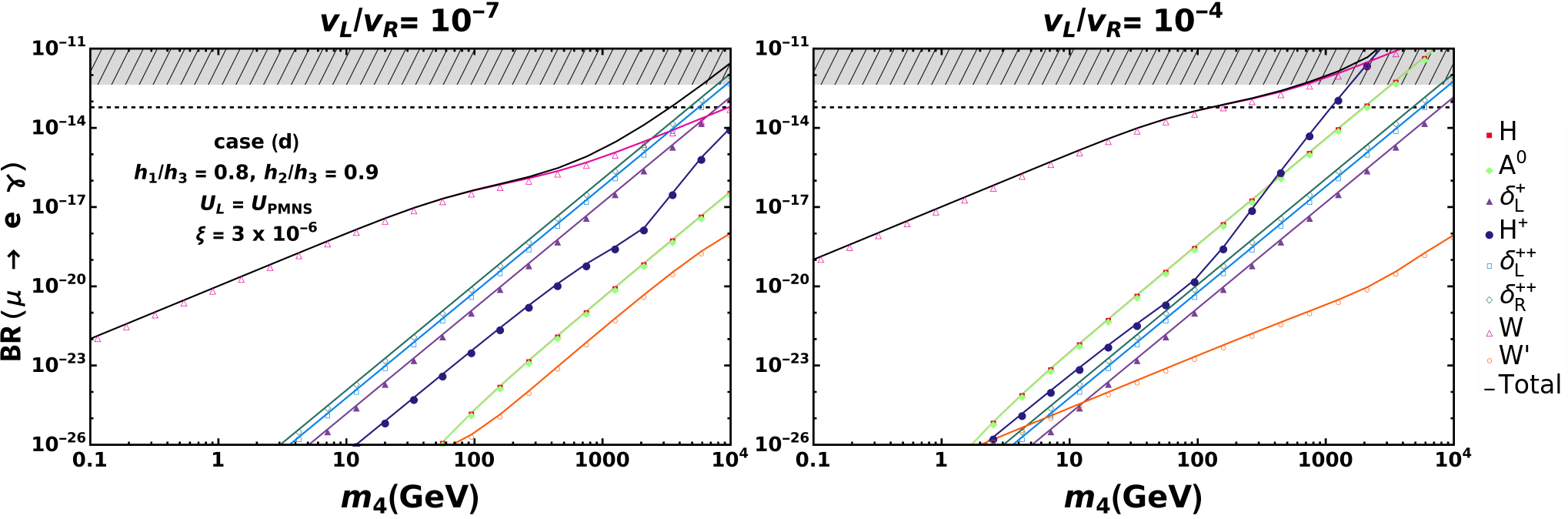
Figure 3: Contributions to the BR$(\mu\to e\gamma)$ in the MLRSM for the parameters of cases (b), (c) and (d). We show the behavior for an intermediate ratio $v_{L}/v_{R}=10^{-7}$ (left panels) and for a larger one $v_{L}/v_{R}=10^{-4}$ (right panels) as a function of $m_{4}$. The gray region is already excluded at 90% CL by the current limit on BR($\mu\to e\gamma$) by the MEG experiment MEG:2016leq , the dashed line shows the sensitivity of $6\times 10^{-14}$, the goal of an upgraded version of MEG Baldini:2013ke .

3.3.2 Three body charged lepton decays

The MLRSM has three kinds of terms that can contribute to charged LFV three body decays such as $\mu\to 3e$, $\tau\to 3e$ or $\tau\to 3\mu$: tree-level contributions, 1-loop contributions and interference (see figure 4).

(a) Tree-level $\mu\to 3e$ decay.

(b) $\mu\to 3e$ through photon exchange.

Figure 4: Different contributions to $\mu\rightarrow 3e$ decay.

The tree-level contributions, which are not present in the standard case, take place through the exchange of the scalars $\delta_{L,R}^{++}$ and can be written as

$$\Gamma(\ell\to 3\ell^{\prime})_{\delta_{R}^{++}}^{\rm{(tree)}} = \frac{m_{\ell}^{5}\left|\left(U_{R}^{*}\,\tilde{h}_{M}\,U_{R}^{\dagger}\right)_{\ell\ell^{\prime}}\left(U_{R}\,\tilde{h}_{M}^{*}\,U_{R}^{T}\right)_{\ell^{\prime}\ell^{\prime}}\right|^{2}}{3\,(32)^{2}\,\pi^{3}\,m_{\delta_{R}^{++}}^{4}}$$ (57)

$$= \frac{m_{\ell}^{5}\left|\left(U_{R}^{*}\,M_{R}\,U_{R}^{\dagger}\right)_{\ell\ell^{\prime}}\left(U_{R}\,M^{*}_{R}\,U_{R}^{T}\right)_{\ell^{\prime}\ell^{\prime}}\right|^{2}}{3\,(64)^{2}\,\pi^{3}\,m_{\delta_{R}^{++}}^{4}v_{R}^{4}},$$

with $\Gamma(\ell\to 3\ell^{\prime})_{\delta_{L}^{++}}^{\rm{(tree)}}$ obtained through the exchanges $U_{R}\rightarrow U_{L}$, $m_{\delta_{R}^{++}}\rightarrow m_{\delta_{L}^{++}}$ and $\tilde{h}_{M}\rightarrow h_{M}$. The 1-loop induced diagrams contain a vertex that has the same structure of the $l\rightarrow l^{\prime}\gamma$ one, so the general decomposition given in eq. (95) holds and we can write their part of the partial width as Kuno:1999jp ; Cornella:2019uxs

$$\Gamma(\ell\to 3\ell^{\prime})_{\gamma} = \frac{\alpha^{2}m_{\ell}^{5}}{48\,\pi}\left\{3\left(\left|\derivative{F_{1}(0)}{q^{2}}\right|^{2}+\left|\derivative{G_{1}(0)}{q^{2}}\right|^{2}\right)\right.$$ (58)

$$- \left.\frac{12}{m_{\ell}^{2}}\left(\text{Re}\left[\derivative{F_{1}(0)}{q^{2}}\,F_{2}(0)^{*}\right]-\text{Re}\left[\derivative{G_{1}(0)}{q^{2}}\,G_{2}(0)^{*}\right]\right)\right.$$

$$+ \left.\frac{8}{m_{\ell}^{4}}\left(\left|F_{2}(0)\right|^{2}+\left|G_{2}(0)\right|^{2}\right)\left(\ln{\frac{m_{\ell}^{2}}{m_{\ell^{\prime}}^{2}}}-\frac{22}{8}\right)\right\}\,,$$

where $F_{1,2}(0)$ and $G_{1,2}(0)$ are four electromagnetic form factors (see appendix B) and we assumed $m_{\ell}\gg m_{\ell^{\prime}}$. Finally the term $\Gamma(\ell\to 3\ell^{\prime})_{\rm{interf.}}$ is the interference term between tree-level and loop level contributions. The full decay width is

$$\Gamma(\ell\to 3\ell^{\prime})=\Gamma(\ell\to 3\ell^{\prime})_{\gamma}+\Gamma(\ell\to 3\ell^{\prime})_{\delta_{R}^{++}}^{\rm{(tree)}}+\Gamma(\ell\to 3\ell^{\prime})_{\delta_{L}^{++}}^{\rm{(tree)}}+\Gamma(\ell\to 3\ell^{\prime})_{\rm{interf.}}\,.$$

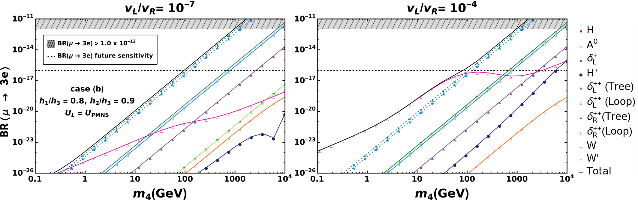
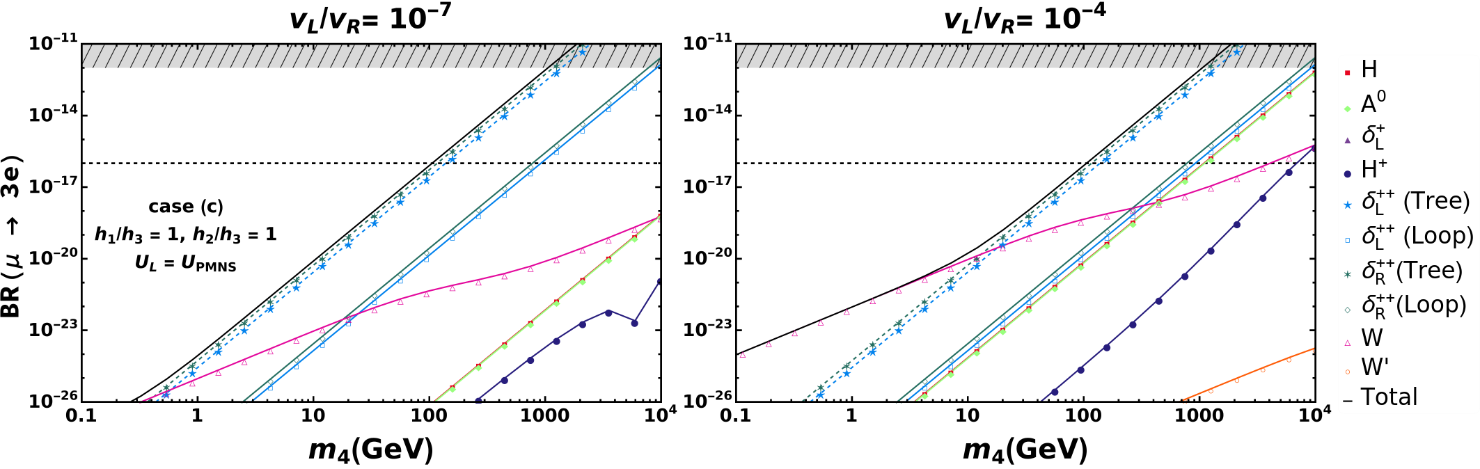
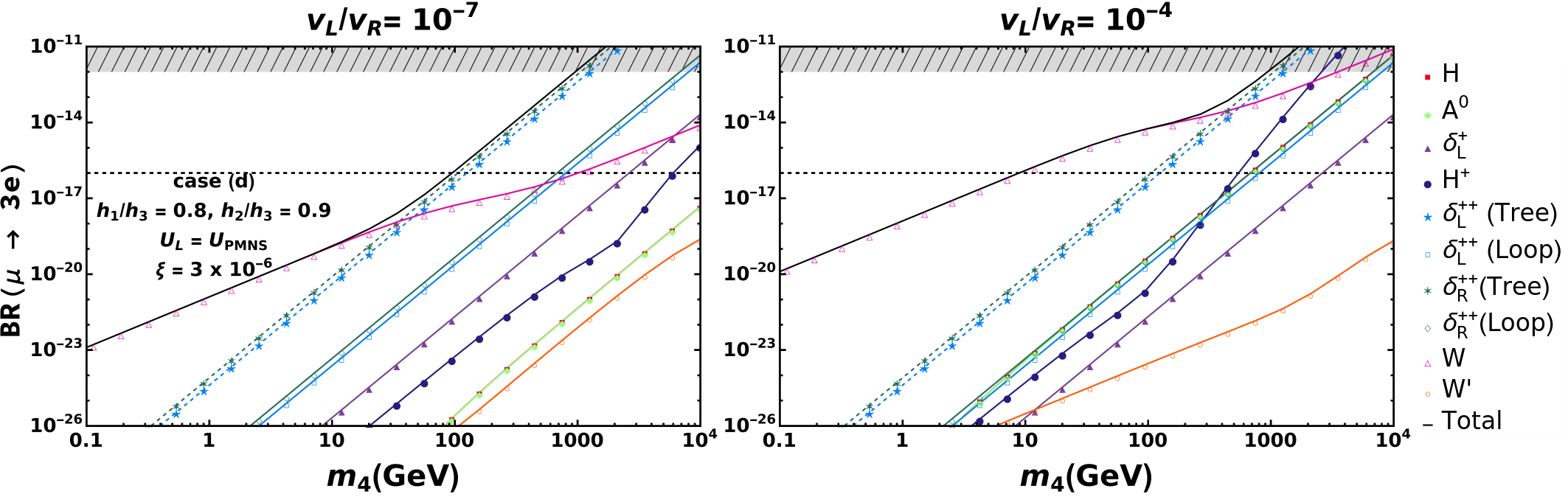
Figure 5: Contributions to BR$(\mu\to 3e)$ in the MLRSM for the parameters of cases (b), (c) and (d). We show the behavior for an intermediate ratio $v_{L}/v_{R}=10^{-7}$ (left panels) and for a large one $v_{L}/v_{R}=10^{-4}$ (right panels) as a function of $m_{4}$. The gray region is already excluded at 90% CL by the current limit on BR($\mu\to 3e$) by the SINDRUM experiment SINDRUM:1987nra , the dashed line shows the sensitivity of the future Mu3e experiment Mu3e:2020gyw .

In figure 5 we illustrate the behavior of each MLRSM contribution to BR$(\mu\to 3e)$ for the same benchmark cases (b) (top panels), (c) (middle panels) and (d) (bottom panels) of table 3 and the same two $v_{L}$ values as in figure 3. We also show the current experimental limit on BR$(\mu\to 3e)<1.0\times 10^{-12}$ SINDRUM:1987nra as well as the expected future sensitivity BR$(\mu\to 3e)=1.0\times 10^{-16}$ Mu3e:2020gyw , for reference. We see that although the $W$ curve is similar with respect to figure 3, in contrast to BR$(\mu\to e\gamma)$, in all cases the double-charged scalar contributions $\delta_{L,R}^{++}$ always become dominant. For larger $\xi$ (case (d)), it will surpass the $W$ contribution as $m_{4}$ increases. This will happen, nevertheless, at lower values of $m_{4}$ than the corresponding cases (b) and (d) of figure 3. Here there is no suppression of the double-charged scalar contributions when heavy neutrinos are degenerate as compared to the case for $\mu\to e\gamma$ because of the presence of the tree level diagrams. Again the current limit can exclude only a small part of the parameter space of the model, but this could increase substantially in the future.

3.3.3 $\mu\to e$ conversion in nuclei

The MLRSM also has several 1-loop contributions to $\mu^{-}+A(N,Z)\to e^{-}+A(N,Z)$, where $A(N,Z)$ is a nucleus with $Z$ protons and $N$ neutrons. The experimental limits shown in table 5 are given on the ratio

$$B^{\rm A}_{\mu\to e}=\frac{\sigma(\mu^{-}A\to e^{-}A)}{\sigma(\mu^{-}A\to{\rm capture})}\,,\quad\quad A\rm={Ti,Au,\;and\;Pb}\,.$$ (59)

Process	Experimental Limit	Reference
$B^{\rm Ti}_{\mu\to e}$	$<4.3\times 10^{-12}$	SINDRUMII:1993gxf
$B^{\rm Au}_{\mu\to e}$	$<7.0\times 10^{-13}$	SINDRUMII:2006dvw
$B^{\rm Pb}_{\mu\to e}$	$<4.6\times 10^{-11}$	SINDRUMII:1996fti

Table 5: Limits from the SINDRUM-II experiment at PSI on the rate of $\mu\to e$ conversion on nuclei at 90% CL.

Figure 6: Contributions to $B^{\rm Al}_{\mu\to e}$ in the MLRSM for the parameters of cases (b), (c) and (d). We show the behavior for an intermediate ratio $v_{L}/v_{R}=10^{-7}$ (left panels) and for a large one $v_{L}/v_{R}=10^{-4}$ (right panels) as a function of $m_{4}$. The gray region is already excluded at 90% CL by the SIMDRUM-II limit on $B^{\rm Au}_{\mu\to e}$ SINDRUMII:2006dvw . We also show the future sensitivity of COMET-I (dashed line), COMET-II (dotted-line) and PRISM (dash-dotted line) COMET:2018auw .

Figure 7: $\mu\to e$ conversion in nuclei through photon exchange.

Here we are going to consider the 1-loop contributions through photon exchange with the nucleus (see figure 7). Again we have the same structure for the vertex as in eq. (95), so the general contribution can be written as Kuno:1999jp

$$B_{\mu\rightarrow e}^{\text{A}}=\frac{8\,V^{(p)\,2}\,e^{4}}{m_{\mu}^{4}\,\Gamma_{\text{cap.}}}\left(\left|F_{1}(-m_{\mu}^{2})+F_{2}(-m_{\mu}^{2})\right|^{2}+\left|G_{1}(-m_{\mu}^{2})+G_{2}(-m_{\mu}^{2})\right|^{2}\right),$$ (60)

where $\Gamma_{\rm cap.}$ is the capture rate of the nucleus considered, $F_{1}(-m_{\mu}^{2}),\,F_{2}(-m_{\mu}^{2}),$ $G_{1}(-m_{\mu}^{2})$, $G_{2}(-m_{\mu}^{2})$ are the form factors evaluated at $q^{2}=-m_{\mu}^{2}$ and $V^{(p)}$ is a number that depends on the atomic number $Z$, the proton density, and the muon and electron wave functions. In the literature we found different methods of evaluating these contributions. This can be done either by using directly the form factors evaluated at $q^{2}=-m_{\mu}^{2}$ or employing a first order expansion for the form factors $F_{2}(-m_{\mu}^{2})\approx F_{2}(0)$, $G_{2}(-m_{\mu}^{2})\approx G_{2}(0)$ and $F_{1}(-m_{\mu}^{2})\approx-m_{\mu}^{2}\,dF_{1}(0)/dq^{2}$, $G_{1}(-m_{\mu}^{2})\approx-m_{\mu}^{2}\,dG_{1}(0)/dq^{2}$. We have checked that both ways are consistent and the numerical difference is negligible. To compute $B_{\mu\rightarrow e}^{\text{A}}$ here we used the values of $V^{(p)}$ and $\Gamma_{\rm cap.}$ given in table 6, taken from Kitano:2002mt .

There are two very aggressive experiments in the near future. COMET is an experiment at J-PARC in Japan which will operate with an Al target and is planed to have two phases: COMET-I which is supposed to achieve a sensitivity on $B^{\text{Al}}_{\mu\to e}$ of $7\times 10^{-15}$ and COMET-II which will bring the sensitivity further down to $2.6\times 10^{-17}$ COMET:2018auw . A third phase, known as PRISM, is under investigation aiming to a sensitivity of $7\times 10^{-19}$. The other facility is Mu2e at Fermilab in the US. This experiment also aims to reach a sensitivity of $10^{-16}$ on $B^{\text{Al}}_{\mu\to e}$ Mu2e:2014fns .

In figure 6 we show the general behavior of the various MLRSM contributions to $B_{\mu\rightarrow e}^{\text{Al}}$ as a function of $m_{4}$ for the same cases of figures 3 and 5. We also show the region excluded by $B^{\text{Au}}_{\mu\to e}<7.0\times 10^{-13}$ as well as the future sensitivities of COMET-I, COMET-II and PRISM. Here again in both cases $\delta_{L,R}^{++}$ surpass the $W$ curve at some point. This happens at about the same values of $m_{4}$ as that for BR$(\mu\to 3e)$. There is again, as expected, no suppression of the double-charged scalars when neutrinos are degenerate as opposed to BR$(\mu\to e\gamma)$. We see that the current bound can exclude only a very modest part of the parameter space of the model, but this could increase very substantially in the future.

Nucleus	$V^{(p)}\,(\text{{\tiny$\times$}}\,m_{\mu}^{5/2})$	$\Gamma_{\rm cap.}\,({\rm eV})$
Au	0.0974	8.60 $\times$ $10^{-9}$
Al	0.0161	4.64 $\times$ $10^{-9}$

Table 6: Values of $V^{(p)}$ in units of $(m_{\mu}^{5/2})$ and $\Gamma_{\rm cap.}$ obtained from Kitano:2002mt .

3.4 Anomalous magnetic moment of the muon ($a_{\mu}$)

Figure 8: Generic diagram depicting the contributions to the anomalous magnetic moment of the muon.

The MLRSM contributions to the anomalous magnetic moment of the muon, $a_{\mu}\equiv(g-2)_{\mu}/2$, can be evaluated by calculating the form factor that enters in the vertex correction diagrams like the one depicted in figure 8 and is given by $a_{\mu}=F_{2}(0)$. In the SM $a_{\mu}^{\text{SM}}=4116591810(43)\times 10^{-11}$ Aoyama:2020ynm , while the latest measurement by the Fermilab National Accelerator Laboratory (FNAL) Muon g-2 Experiment found $a_{\mu}^{\text{FNAL}}=116592040(54)\times 10^{-11}$ Muong-2:2021ojo , which combined with previous experimental results lead to $\Delta a_{\mu}\equiv a_{\mu}^{\text{exp}}-a_{\mu}^{\text{SM}}=(251\pm 59)\times 10^{-11}$.

Figure 9: Contributions to $|a_{\mu}|$ in the MLRSM in standard case (a) for $v_{L}/v_{R}=10^{-7}$ (left panel) and $v_{L}/v_{R}=10^{-4}$ as a function of $m_{4}$. The red (light red) region represents the value needed to explain $a_{\mu}^{\rm exp}$ within 2$\sigma$ (3$\sigma$) Muong-2:2021ojo . The solid (dashed) lines represent positive (negative) contributions.

In figure 9 we show the various contributions to $|a_{\mu}|$ as a function of $m_{4}$ for case (a). The total contribution which is overall positive, except for $m_{4}\gtrsim 1$ TeV, is dominated by the $W$ (for $m_{4}\lesssim 10$ keV) or by the $W^{\prime}$ (for $10$ keV $\lesssim m_{4}\lesssim 1$ TeV) exchange. The $W^{\prime}$ contribution is independent of $v_{L}$ and of $m_{4}$ but it is about three to four orders of magnitude smaller than what is needed to explain $a_{\mu}^{\rm exp}$. Except for the contributions from $W^{\prime}$, $W$ and $H^{+}$, the other contributions are always negative, so they cannot help to decrease the discrepancy between theory and experiment. In particular, for $m_{4}\gtrsim 1$ TeV, the dominant contributions, from charged scalars ($\delta_{R,L}^{++},\delta_{L}^{+}$), are all negative, but still too small to make any significant measurable effect.

3.5 Electric dipole moment ($d_{\ell}$)

Now we will examine the status of the electric dipole moment $d_{\ell},\ell=e,\mu$. In the case of the electron’s electric dipole moment (eEDM) $d_{e}$, the ACME II collaboration used a beam of ThO molecules to set the best limit to date at $|d_{e}|<1.1\times 10^{-29}$ e$\cdot$cm ACME:2018yjb . The NL-eEDM collaboration NL-eEDM:2018lno claims a sensitivity of $5\times 10^{-30}$ e$\cdot$cm on $|d_{e}|$ is feasible using an intense primary cold source of barium monofluoride molecules. There is an even more daring proposition, the authors of ref. Fitch:2020jil affirm that using ultracold YbF molecules trapped in an optical lattice one can hope to bring down the sensitivity to the level of $(10^{-31}-10^{-32})$ e$\cdot$cm.

For $d_{\mu}$ the most stringent limit $|d_{\mu}|<1.8\times 10^{-19}$ e$\cdot$cm was set by the BNL Muon $g-2$ experiment Muong-2:2008ebm . The $g-2$ experiments at Fermilab and at J-PARC aim to achieve a similar sensitivity of $|d_{\mu}|\sim 10^{-21}$ e$\cdot$cm Chislett:2016jau ; Abe:2019thb . There are also plans to have a dedicated experiment using a frozen-spin technique at PSI to try to bring down the sensitivity to $|d_{\mu}|\sim 6\times 10^{-23}$ e$\cdot$cm Adelmann:2021udj ; Sakurai:2022tbk . J-PARC also proposed a dedicated experiment that claims to reach $|d_{\mu}|\sim 10^{-24}$ e$\cdot$cm Farley:2003wt .

Theoretically

$$|d_{\ell}|\equiv\frac{|G_{2}(0)|}{(2\,m_{\ell})}\,\rm e\,,$$ (61)

which can in the MLSRM be enhanced by phases in $M_{R}$ or in $U_{L}$. For the approximate expressions for $d_{\ell}$ see appendix B. However, only $|d_{e}|$ can be significantly enhanced to reach values of the order of the current bound. The particles that impact this observable in the model are the vector bosons $W$ and $W^{\prime}$, the charged scalar $H^{+}$ and the neutral scalars $H,A^{0}$.

Figure 10: Contributions to $|d_{e}|$ in the MLRSM for the parameters of cases (a) but with $\phi_{1}=\pi/2$, (c) and (d). We show the behavior for an intermediate ratio $v_{L}/v_{R}=10^{-7}$ (left panels) and for a large one $v_{L}/v_{R}=10^{-4}$ (right panels) as a function of $m_{4}$. The solid (dashed) lines represent positive (negative) values of $d_{e}$. The gray region is already excluded at by the ACME II collaboration ACME:2018yjb , while the dashed line show the possible reach of the NL-eDM experiment using BaF molecules NL-eEDM:2018lno .

In figure 10 we show the various contributions of the model to $|d_{e}|$ as a function of $m_{4}$ for $v_{L}/v_{R}=10^{-7}$ (left panel) and $v_{L}/v_{R}=10^{-4}$ (right panel) for the case (a) but with $\phi_{1}=\pi/2$ (top panels) and for case (c) (middle panels) and case (d)(bottom panels). We observe that case (a) with $\phi_{1}=\pi/2$ and case (d) where $U_{L}=U_{\rm PMNS}$ and larger mixing $\xi$ produce similar constraints on $|d_{e}|$. The contribution of $H^{+}$ for small $m_{4}$ is dominated by the couplings that depend on $M_{\ell}$ (see eqs. (126) and (127)) and, depending on $\phi_{R}$, can change the sign when crossing the transition region from the type-I seesaw to the tuned regime due to the change of behavior of $M_{D}$. On the other hand, for big $m_{4}$, contributions of $H^{+}$ that grow with the heavy neutrino mass become important and dominate. Among those there are two different combinations of couplings that generate $d_{e}$’s with opposite signs and what dictates which one dominates is the value of $|U_{\alpha i}|^{2}\sim v_{L}/v_{R}$, see for example case (c) in figure 10. Regarding the neutral scalars $H$ and $A^{0}$, their contributions are the same but with opposite signs so even when their individual contributions have sizable effect, they cancel each other when summed. In case (c) since $\xi$ is two orders of magnitude smaller than in case (d) the limit is weakened in the same proportion. We do not show case (b) as it is very similar to case (c).

In figure 11 we show the region in the plane $m_{4}\times\phi_{1}$ excluded by the current limit on $|d_{e}|$ with the remaining parameters fixed as in case (a). It is interesting to notice that it is not very dependent on the exact value of the phase $\phi_{1}$, as long as $\frac{\pi}{50}\lesssim\phi_{1}\lesssim\frac{49\pi}{50}$, away from the CP-conserving values.

Besides the case where both $U_{L}=\mathbf{I}$ and $\phi_{1}\neq 0$, the maximum contributions to $|d_{\mu}|$ are similar to those for $|d_{e}|$ and so do not reach a value that can be probed by neither current nor future experiments. When $U_{L}=\mathbf{I}$ and $\phi_{1}\neq 0$ only the imaginary part of the electron couplings are affected, keeping the muon contributions untouched and therefore suppressed. In order to modify the imaginary part of the muon couplings keeping $U_{L}=\mathbf{I}$, the phase $\phi_{2}$ needs to be invoked, though the maximum value $|d_{\mu}|$ achieved is still well below experimental reach.

Figure 11: Region in the plane $m_{4}\times\phi_{1}$ excluded by the current limit on $|d_{e}|$ ACME:2018yjb for the case (a) with varying $\phi_{1}$, we also show by a dashed line the expected sensitivity for a future experiment NL-eEDM:2018lno . The panel on the left (right) is for $v_{L}/v_{R}=10^{-7}$ ($v_{L}/v_{R}=10^{-4}$).

3.6 $W$ boson mass

Finally, we would like to address the influence the exact value of $m_{W}$ has on the model parameters used in our study. The recent analysis of CDF II data resulted on a new value for the $W$ boson mass CDF:2022hxs

$$m_{W}^{\textrm{CDF}} = \left(80.4335\pm 0.0094\right)\,{\rm GeV},$$ (62)

which is in 7$\sigma$ tension with the SM prediction $m_{W}^{\textrm{SM}}=\left(80.361\pm 0.006\right)$ GeV from a global electroweak fit ParticleDataGroup:2020ssz .

The shift in the $W$ boson mass from the SM value $m_{W}^{\textrm{SM}}$ can be written in terms of $S$, $T$, $U$ parameters Peskin:1990zt ; Peskin:1991sw as Maksymyk:1993zm

$$m_{W} = m_{W}^{\rm SM}\left[1-\frac{\alpha S}{2\left(c_{W}^{2}-s_{W}^{2}\right)}+\frac{c_{W}^{2}\alpha T}{c_{W}^{2}-s_{W}^{2}}+\frac{\alpha U}{4s_{W}^{2}}\right]^{1/2},$$ (63)

where $s_{W}$ is the sine of the Weinberg angle, i.e., $s_{W}^{2}=0.2351$ ($c_{W}^{2}=1-s_{W}^{2}$) and the fine structure constant $\alpha=1/128.18$ is taken at the $Z$ boson mass scale $m_{Z}$. The $W$ boson mass in the SM electroweak fit is determined from the relation Awramik:2003rn

$$m_{W}^{\textrm{SM}} = m_{Z}\left[\frac{1}{2}+\frac{1}{2}\sqrt{1-\frac{2\sqrt{2}\pi\alpha}{G_{F}m_{Z}^{2}}\left(1+\Delta r\right)}\right]^{1/2},$$ (64)

where $G_{F}$ is the Fermi constant and $\Delta r$ takes into account the radiative corrections. $G_{F}$ is determined from the muon lifetime $G_{F}=G_{\mu}$ which can be sensitive to the nonunitarity of the $U_{\rm PMNS}$ and can affect the determination of $m_{W}^{\textrm{SM}}$. Ref. Blennow:2022yfm showed that a deviation from unitarity of the $U_{\rm PMNS}$ of the order of $10^{-3}$ is required to be consistent with the new result (62) which translates to $\left|\delta U_{L}\right|\sim\left|{\cal U}_{LR}\right|^{2}\sim 10^{-3}$ in our scenario. This possibility is ruled out by neutrinoless double beta observable (see deGouvea:2015euy and also figure 2 of our earlier analysis) and hence will not be considered further.

In the MLRSM, since $v_{L}\ll v_{R}$, the main contributions to $W$ boson mass will come from loop corrections from the left-handed scalar triplet $\mathbf{\Delta}_{L}$ expressed in term of $S$, $T$ and $U$ as in eq. (63). Using the expressions from ref. Lavoura:1993nq , we can determine $S$, $T$ and $U$ with the mass spectrum of the field components of $\mathbf{\Delta}_{L}$

$$m_{\delta_{L}^{0}}^{2} = m_{\delta_{L}^{++}}^{2}-\frac{\alpha_{3}}{2}\kappa_{+}^{2},$$ (65)

$$m_{\delta_{L}^{+}}^{2} = m_{\delta_{L}^{++}}^{2}-\frac{\alpha_{3}}{4}\kappa_{+}^{2},$$ (66)

where $\alpha_{3}$ is a dimensionless coupling in the scalar potential, $m_{\delta_{L}^{0}}^{2}\equiv m^{2}_{H_{L}}=m^{2}_{A_{L}}$ and we recall that $\epsilon=2\kappa_{1}\kappa_{2}/\kappa_{+}^{2}\ll 1$. The contribution to $U$ is in general small and is at the level $\lesssim 10^{-3}$ for our scenario and can be neglected. Furthermore, we find $S<0$ while $T>0$ and that $-S\ll T$. So, the contribution to $W$ mass is essentially determined by $T>0$. In the isospin conserving limit $\alpha_{3}\to 0$, $T\to 0$ and hence one will need a large $\alpha_{3}$ to have a large $T$. This will make the heavy neutral Higges $H$, $A^{0}$ correspondingly heavy since their squared masses are $\alpha_{3}v_{R}^{2}/2$. The $H$, $A^{0}$ and heavy $W^{\prime}$ contributions to $B-\bar{B}$ mixing lead to a lower bound on $\alpha_{3}$ as a function of $m_{W^{\prime}}$ Bertolini:2014sua ; Maiezza:2016bzp

$$\alpha_{3} \approx \frac{30}{\left(m_{W^{\prime}}/2.23\,{\rm TeV}\right)^{2}-1}.$$ (67)

Hence we can express the compatible $S$ and $T$ in terms of $m_{W^{\prime}}$ and $m_{\delta_{L}^{++}}$. Various groups, for example Balkin:2022glu ; Asadi:2022xiy , provide the best-fit for $S$ and $T$ at 1$\sigma$ assuming $U=0$ taking into account the new CDF result (62). In figure 12, we show the $S$ and $T$ parameter space of the MLRSM and the 1 $\sigma$ parameter space that can explain the $W$ mass is obtained from ref. Asadi:2022xiy .

We see that for the model to be compatible with $m_{W}^{\rm CDF}$ we need $m_{W^{\prime}}\sim(5-6)$ TeV and $m_{\delta_{L}^{++}}\sim(0.9-1.4)$ TeV. Both ranges of values are still allowed by experiments.

Figure 12: Contribution to S and T in the MLRSM. The blue and red ellipses are the $2\sigma$ preferred regions from the electroweak fit for the PDG and the new CDF II $m_{W}$ measurent, respectively Asadi:2022xiy .

4 Discussion of Results

Now we will discuss the allowed regions in the plane $v_{L}/v_{R}\times m_{4}$ after imposing the following experimental limits on the model: (a) $m_{\beta\beta}<126$ meV KamLAND-Zen:2022tow ; (b) BR$(\mu\to e\gamma)<4.2\times 10^{-13}$ MEG:2016leq ; (c) BR$(\mu\to 3e)<1.0\times 10^{-12}$ SINDRUM:1987nra ; $B^{\rm Au}_{\mu\to e}<7.0\times 10^{-13}$ SINDRUMII:2006dvw and $|d_{e}|<1.1\times 10^{-29}$ e$\cdot$cm ACME:2018yjb . We have also forced the mixing elements $|U_{\alpha i}|$ to pass the laboratory constraints given in ref. deGouvea:2015euy . We show on the plots the region of the parameter space that can be explored by the future accelerator experiments taken from ref. Ballett:2019bgd . For completeness we also show the BBN limits on $m_{4}\times|U_{\alpha 4}|^{2}$ for $m_{4}$ in the range 3 MeV to 1 GeV taken from ref. Sabti:2020yrt (in teal blue) and on $m_{4}\times\sum_{\alpha}|U_{\alpha 4}|^{2}$ for $m_{4}$ in the range $10^{-8}$ GeV to 1 GeV from an analysis of heavy neutral leptons in consistence with measurements of the Hubble constant, Supernovae Ia luminosity distances, the CMB shift parameter, the BAO scale taken from ref. Vincent:2014rja (in blue grey) .

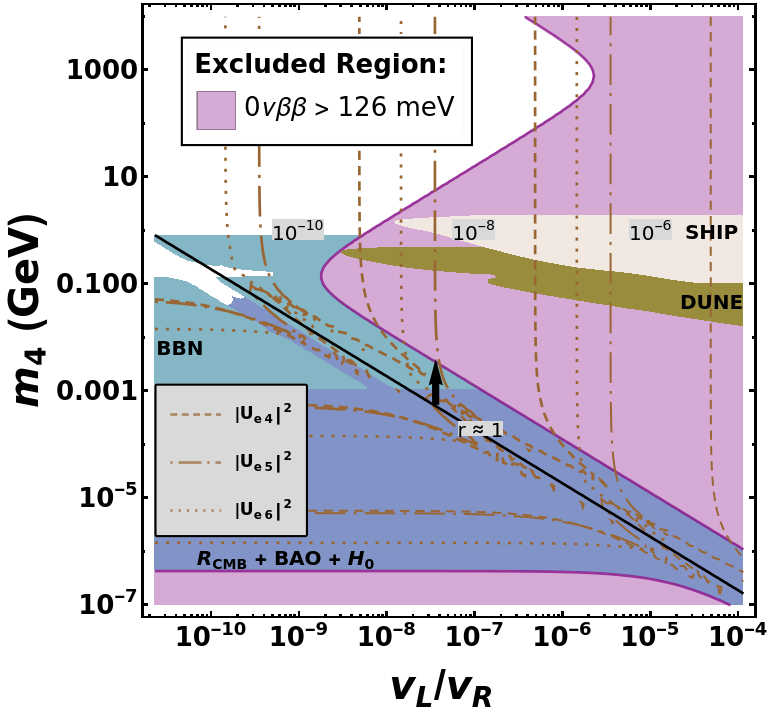
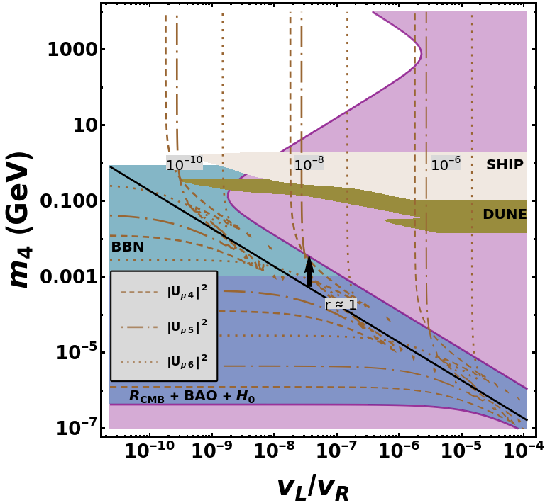
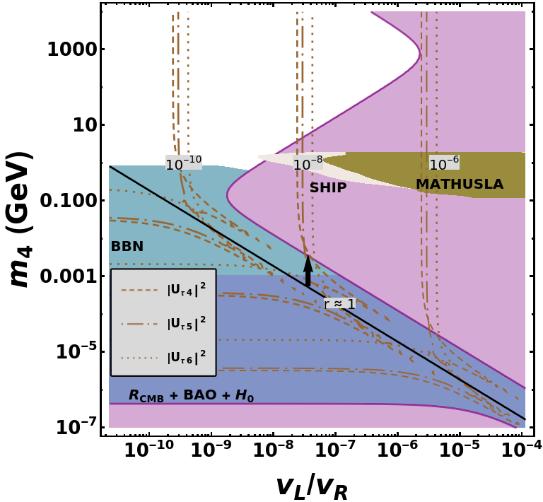
Figure 13: Excluded regions for case (a) by the current bound on $0\nu\beta\beta$ decay (pink) KamLAND-Zen:2022tow , BBN Sabti:2020yrt (teal blue) and other cosmological observables ($H_{0}$, BAO, Supernovae type Ia and the CMB shift parameter) Vincent:2014rja (blue grey). The black line separates the tuned region ($r\sim 1$), above the line, from the type-I seesaw region ($r<1$), below the line. In the top left panel we show lines for $|U_{ei}|^{2}=10^{-10},10^{-8}$ and $10^{-6}$ as dashed ($i=4$), dashed-dotted ($i=5$) and dotted ($i=6$). The same is shown in the top right (bottom) panel for $|U_{\mu i}|^{2}$($|U_{\tau i}|^{2}$). The sensitivity regions for SHIP, DUNE and MATHUSLA were taken from  Ballett:2019bgd .

We will start by looking at the benchmark cases. In these cases we have set $v_{R}$ to the minimum value and $\xi$ to the maximum value for which $0\nu\beta\beta$ decay can restrict the plane $v_{L}/v_{R}\times m_{4}$ the least, in the tuned region. If we increase $v_{R}$ or decrease $\xi$ from their standard values, we have verified that this region will not change. Nevertheless an increase of $v_{R}$ may remove the constraint in the type-I regime. The black diagonal line in the plots separates the tuned regime ($r\sim 1$), the region above this line, from the type-I seesaw ($r<1$), the region below this line.

Figure 14: Excluded regions for case (b). We include the same bounds used in figure 13 as well as the current limits on $\mu\to e\gamma$ MEG:2016leq (red), on $\mu\to 3e$ SINDRUM:1987nra (blue), on $B^{\rm Au}_{\mu\to e}$ SINDRUMII:2006dvw (dark grey) and on $|d_{e}|$ ACME:2018yjb . The expected sensitivity of future LFV and eEDM experiments are shown by the corresponding color line with an arrow.

In figure 13 we see our results for case (a) where the $0\nu\beta\beta$ bound excludes a significant portion of the tuned region as well as a small portion of the type-I seesaw region (below $m_{4}\lesssim 4\times 10^{-7}$ GeV). As previously explained, there are no LFV or $|d_{e}|$ limits for this case. For degenerate neutrinos and $U_{L}=\mathbf{I}$, in the tuned region all matrix elements $|U_{\alpha i}|^{2},i=4,5,6$ are of the order $(v_{L}/v_{R})|\phi_{R}|^{2}$ (see eqs. (28)) and (24)). In the top left panel we show lines of constant $|U_{ei}|^{2}=10^{-10},10^{-8}$ and $10^{-6}$, as dashed ($i=4$), dashed-dotted ($i=5$) and dotted ($i=6$), for reference. In the top right (bottom) panel the same is shown for $|U_{\mu i}|^{2}$ ($|U_{\tau i}|^{2}$ ). These lines are independent of $v_{L}/v_{R}$ in the type-I seesaw region and in the transition there is a cancellation which corresponds to one of the three light neutrino masses $m_{1}$, $m_{2}$ or $m_{3}$ . We also show the expected sensitivity of the accelerator experiments most effective to probe each of those mixing matrix elements according to Ballett:2019bgd . The cosmological limits exclude the entire type-I seesaw region and a small part of the tuned region that was not excluded by $0\nu\beta\beta$. In the parameter space still allowed all the elements $|U_{\alpha i}|^{2}\lesssim 10^{-5}$.

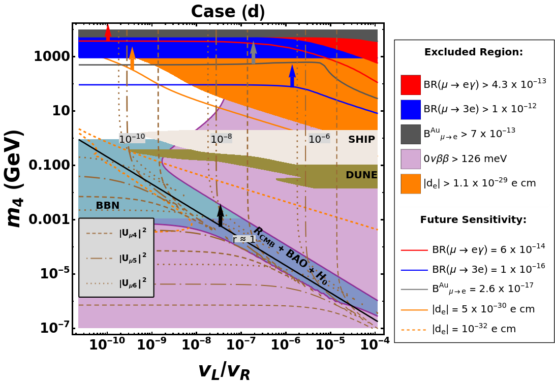
Figure 15: Same as figure 14 but for case (d).

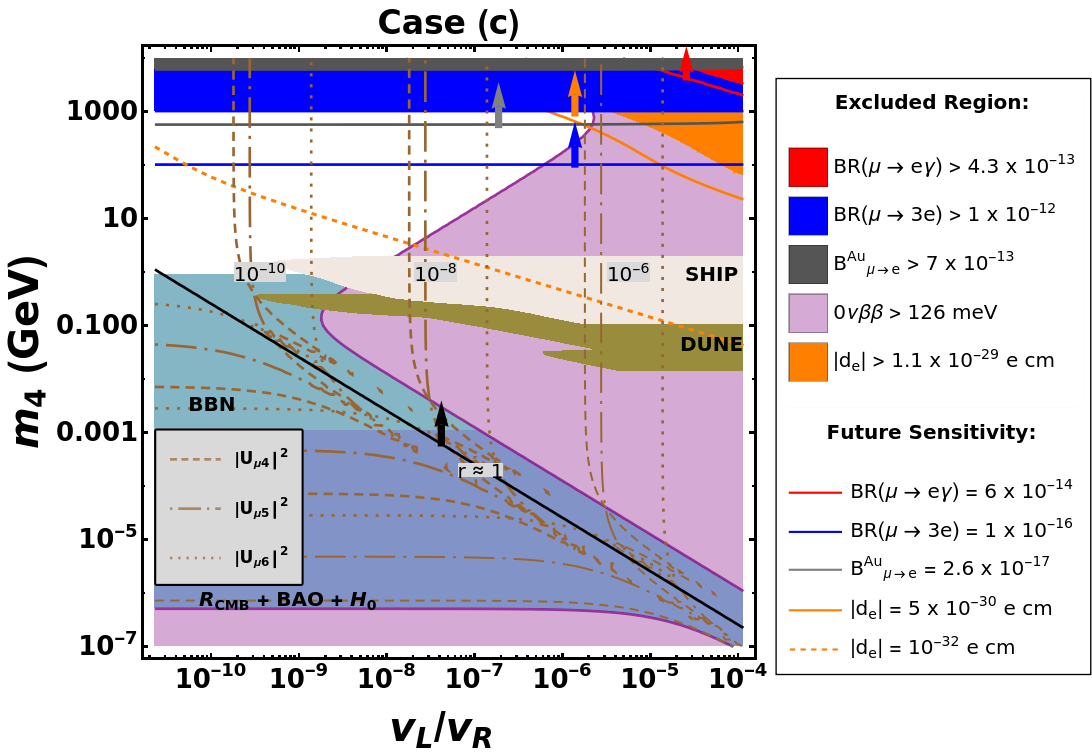
Figure 25: Case (c) where $\phi_{i}=0$.

In case (b), shown in figure 14, $U_{L}\neq\mathbf{I}$ and the heavy neutrinos are mildly hierarchical. We observe that the limits from $0\nu\beta\beta$ are not affected by this choice due to the low value we took for the mixing $\xi$, but there are now limits from LFV. These limits concern exactly the part of the tuned region that is free from cosmological constraints. The reach of some of the future charged LFV experiments is also shown in this figure. They have the potential to probe a significant portion of the parameter space still allowed in the tuned region. The current bound on $|d_{e}|$ excludes regions that are already not allowed by $0\nu\beta\beta$ decay or LFV. Here we only show lines of constant $|U_{\mu i}|^{2}$ as for the top right panel of figure  13. In the tuned region all matrix elements $|U_{\alpha i}|^{2}$ are of the order $v_{L}/v_{R}|U_{L}|^{2}$. In the region still allowed all the elements $|U_{\alpha i}|^{2}\lesssim 10^{-6}$ ($v_{L}\lesssim 200$ MeV). We do not show explicitly case (c) here, as it is very similar to (b), so the heavy neutrino mass hierarchy does not play a significant role. See figures 25 in appendix C.

In figure 15 we can see that case (d) is qualitatively similar to (b), however, the larger value of $\xi$ results in a larger area excluded by $0\nu\beta\beta$ decay, most notably in the type-I seesaw region, but also in the tuned one. Due to this the LFV bounds also increase for $v_{L}/v_{R}\gtrsim 10^{-5}$ (the $W$ term is enhanced by the larger mixing $\xi$ ), covering a part of the parameter space already excluded by $0\nu\beta\beta$ decay. In the window still allowed by data we have all the elements $|U_{\alpha i}|^{2}\lesssim 10^{-8}$ ($v_{L}\lesssim 2$ MeV). Likewise the eEDM limits becomes more significant in this case, already excluding part of the parameter space in the reach of future LFV experiments, in particular, $v_{L}/v_{R}\gtrsim 10^{-7}$ is discarded.

Figure 16: Same as figure 13 but for $v_{R}=11$ TeV.

Let us discuss now the impact of changing the value of one of the fixed parameters of case (a) on our results:

1. decrease $v_{R}$: lower values of $v_{R}$ will increase the part of the parameter space excluded by $0\nu\beta\beta$ decay (as $\lambda\propto v_{R}^{-2}$), specially in the tuned region, but also in the type I seesaw regime. This is mainly due to the contributions $RR,N$, that is independent of $v_{L}/v_{R}$, and $RL,\lambda$ (see figure 1) which increases as $v_{L}/v_{R}\to 0$. In figure 16 we illustrate this effect for $v_{R}=$ 11 TeV ($m_{W^{\prime}}=5$ TeV). The only region that still survives is $m_{4}\gtrsim 10$ GeV and $v_{L}/v_{R}\lesssim 3\times 10^{-7}$. If $U_{L}\neq\mathbf{I}$, LFV bounds would restrict the allowed region even further.

2. change $U_{L}$: different $U_{L}$ can have two effects: modify the $0\nu\beta\beta$ decay exclusion regions, connecting them in the transition region, and increasing the bounds from LFV and eEDM processes excluding lower values of $m_{4}$. In figure 17 we show an example for a random unitary $U_{L}$ where we see how the LFV and eEDM bounds can be more restrictive depending on $U_{L}$.

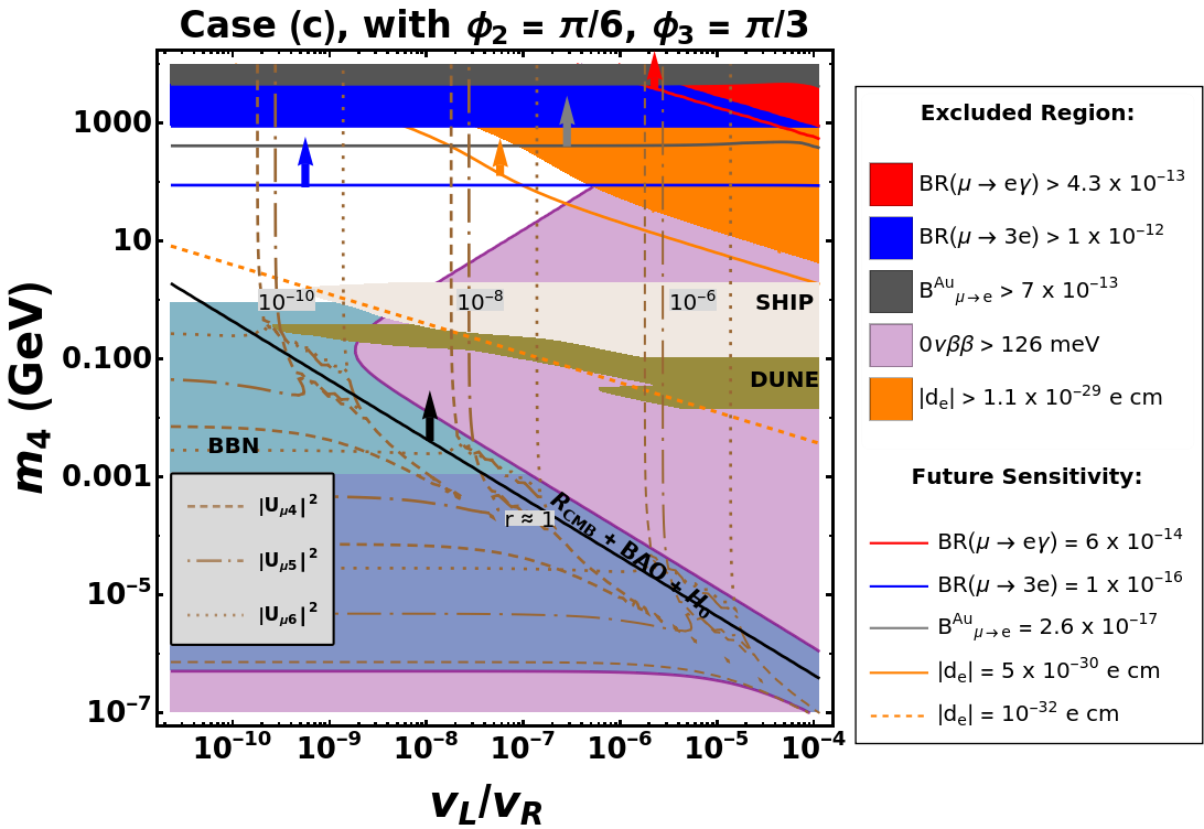
Figure 26: Case (c) with $\phi_{2}=\pi/6$ and $\phi_{3}=\pi/3$.

3. change $\phi_{i}$: when $U_{L}\neq\mathbf{I}$ the effect of the extra phases in $M_{R}$ is somewhat degenerate with the phases in $U_{L}$ (see figure 26 in appendix C), nevertheless, when $U_{L}=\mathbf{I}$, $\phi_{1}\neq 0$ can produce sizable $|d_{e}|$. In figure 18 we illustrate this effect for the case (a) with $\phi_{1}=\pi/2$ while $\phi_{2}=\phi_{3}=0$. We see that eEDM and $0\nu\beta\beta$ rule out $v_{L}/v_{R}\gtrsim 10^{-7}$.

   

   Figure 17: Same as figure 13 but for a random $U_{L}$.

   

   Figure 18: Same as figure 13 but with $\phi_{1}=\pi/2$.

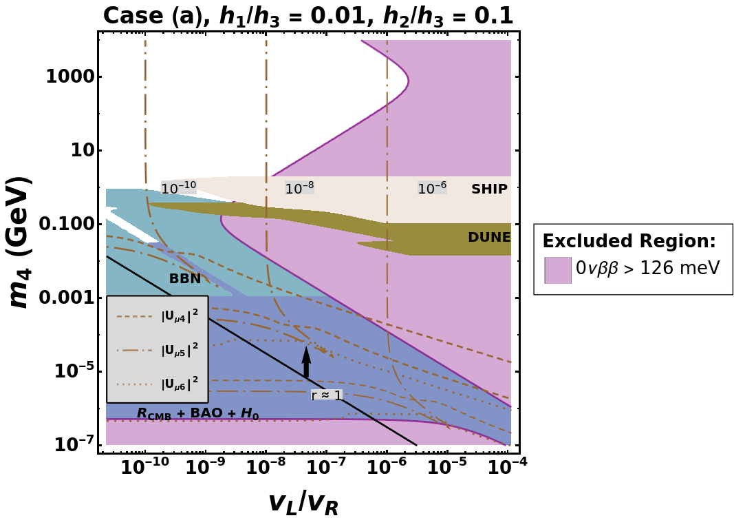
Figure 21: Case (a) for a different heavy neutrino mass hierarchy.

4. change the heavy neutrinos mass hierarchy: the results are basically unaffected by the assumed heavy neutrinos mass hierarchy, the only feature worth mentioning is the fact that for non-degenerate heavy neutrinos and $U_{L}=\mathbf{I}$, in the tuned region the $U_{\alpha i}$ matrix is diagonal, i.e., we will only have $|U_{e4}|^{2}=|U_{\mu 5}|^{2}=|U_{\tau 6}|^{2}=v_{L}/v_{R}$. See figure 21 in appendix C.

5. change the light neutrinos mass scale and mass ordering: this will only affect the mixing matrix $U_{\alpha i}$ in the type-I seesaw region and in the transition zone (for IO or quasi-degenerate we will see two or one cancellation lines). It is worth mentioning that for NO as $m_{0}\to 0$ the $0\nu\beta\beta$ decay exclusion region in the type I seesaw region disappears. See the figures in appendix C.2.

Figure 19: Correlation among the three LFV observables $\mu\to e\gamma$, $B^{\rm Al}_{\mu\to e}$ and $\mu\to 3e$ (color scale). We also show the current limits and the sensitivities expected for experiments in the near future. On the left panel heavy neutrinos are hierarchical and on the right panel we have included also the cases when heavy neutrinos are degenerate.

In the auspicious occurrence of a positive observation of LFV in $\mu\to e\gamma$, $\mu\to 3e$ or $B^{\rm Al}_{\mu\to e}$ in the near future we provide the correlations among these observables in the tuned region in figure 19. We have constructed this plot by varying: $v_{R}=11$ and $44$ TeV, $\xi=(3\times 10^{-8},3\times 10^{-7},3\times 10^{-6})$, $m_{4}\in[1,10^{4}]$ GeV, $v_{L}/v_{R}\in[10^{-10},10^{-4}]$, $(h_{1}/h_{3}$,$h_{2}/h_{3})=\{(1,1),(0.9,0.95),(1/3,1/2),(1/5,1/3)\}$ and $U_{L}=U_{\rm PMNS}$ and 4 other different random unitary matrices for $U_{L}$. On the left panel we consider only the cases when heavy neutrinos are hierarchical with $(h_{1}/h_{3}$, $h_{2}/h_{3})$ = $\{(0.9,0.95),$ $(1/3,1/2),(1/5,1/3)\}$ and on the right panel we consider all mentioned cases including degenerate heavy neutrinos when $(h_{1}/h_{3}$, $h_{2}/h_{3})=(1,1)$. The correlation between $\mu\to e\gamma$ and $B^{\rm Al}_{\mu\to e}$ decreases when heavy neutrinos are degenerate and the left-right mixing $\xi$ is smaller. In particular for $\xi=3\times 10^{-8}$ it is possible to have $B^{\rm Al}_{\mu\to e}\sim 10^{-15}$ while having BR$(\mu\to e\gamma)\lesssim 10^{-23}$.

We see that we can have $\mu\to 3e$ and $B^{\rm Al}_{\mu\to e}$ sizable, well within the reach of future experiments, while having $\mu\to e\gamma$ much bellow the future experimental sensitivity of MEG-II. This is even more so if heavy neutrinos are degenerate. The reason being the fact that $\mu\to e\gamma$ depends only on the form factors $F_{2}$ and $G_{2}$ and these for the doubly scalar contributions are, at leading order, suppressed when $M_{R}$ is proportional to the identity (see, for instance, case (c) in figure 3). This is not true for the other processes. But if MEG-II observes a signal, $\mu\to 3e$ must be observed with BR$(\mu\to 3e)\lesssim 10^{-14}$. However, in this case COMET-I may not observe anything, while COMET-II must see something. On the other hand, if COMET-I (or COMET-II) observe a signal, $\mu\to 3e$ must be around the corner, then again, in this case MEG-II may not observe anything. Finally, if $\mu\to 3e$ is observed it will tell us where to look for $\mu\to e\gamma$ and $B^{\rm Al}_{\mu\to e}$.

5 Conclusions

We have explored the neutrino sector of the MLRSM, in particular, in the tuned regime where type-I and type-II seesaw mechanisms supply similar contributions to neutrino masses. We have discussed how to parametrize and reconstruct the neutrino mass matrix in the general case as well as under ${\cal C}$ and ${\cal P}$ discrete symmetries.

Imposing the model to be additionally invariant under ${\cal C}$ discrete symmetry, we have reconstructed and diagonalized neutrino mass matrices, subject to several assumptions on the heavy neutrino sector, which are compatible with the requirements of the light neutrino sector: the mass squared differences and mixing angles indicated by neutrino oscillation data, KATRIN limits and the cosmological bound on the sum of light neutrino masses. The unknowns in the light neutrino sector ($m_{0}$, mass ordering, $\delta$, $\alpha_{1,2}$) do not alter our general conclusions.

Fixing the masses of the relevant scalars to the minimum value allowed by data, i.e., $m_{H}=m_{A^{0}}=m_{H^{+}}=$ 15 TeV, $m_{\delta^{+}_{L}}=m_{\delta^{++}_{L}}=780$ GeV and $m_{\delta^{++}_{R}}=660$ GeV, we have investigated for different choices of $U_{L}$, values of $v_{R}$, values of the left-right mixing $\xi$, assumptions on the heavy neutrino mass hierarchy, and on the $\phi_{i}$ phases, the constraints from $0\nu\beta\beta$ decay, $\mu\to e\gamma$, $\mu\to 3e$, $B^{\rm Al}_{\mu\to e}$, $a_{\mu}$ and $|d_{e}|$. For completeness, we have also included BBN and other cosmological limits in our study.

To facilitate the discussion, we have defined four benchmark cases (a)-(d), according to table 3. As the $0\nu\beta\beta$ decay limit depends mostly on $v_{R}$ and $\xi$, we have fixed $v_{R}=44$ TeV and $\xi=3\times 10^{-8}$ at the minimum and maximum values of these parameters, respectively, for which the constraint from $0\nu\beta\beta$ decay exclude the least the parameter space of the model in the plane $v_{L}/v_{R}\times m_{4}$ in the tuned regime. Since the value of $U_{L}$, the heavy neutrino mass hierarchy and the $\phi_{i}$ phases are practically unimportant here, we set $U_{L}=\mathbf{I}$, heavy neutrinos as degenerate and $\phi_{i}=0$ for the benchmark values of our standard case, case (a). In this situation there is no LFV or eEDM, so this particular scenario is the least restrictive for the neutrino sector of the model. Nevertheless, cosmological data and $0\nu\beta\beta$ decay exclude the entire type-I seesaw region and a substantial part of the tuned region for $v_{L}/v_{R}\gtrsim 10^{-11}$. For instance, if $m_{4}=10$ TeV then $v_{L}/v_{R}\lesssim 2\times 10^{-5}$, if $m_{4}=1$ GeV then $v_{L}/v_{R}\lesssim 2\times 10^{-8}$. If $\frac{\pi}{50}\lesssim\phi_{1}\lesssim\frac{49\pi}{50}$, however, the current limit on eEDM does not allow for $v_{L}/v_{R}\gtrsim 10^{-7}$.

In general, we have shown that unless the charged lepton mixing matrix $U_{L}=\mathbf{I}$ and the phases $\phi_{i}$ are all zero, we expect to have sizable LFV and eEDM in the tuned region. This is exemplified by cases (b) and (c) where $U_{L}=U_{\rm PMNS}$, the first with mildly hierarchical, the second with degenerate neutrinos. We have observed that the exact mass hierarchy is not very significant for the final results. Here the non-observation of LFV processes further discard $m_{4}\gtrsim 1$ TeV and imposes $v_{L}/v_{R}\lesssim 5\times 10^{-6}$, with the perspective in the future to probe down to $m_{4}\sim 100$ GeV independent of $v_{L}/v_{R}$. In these cases eEDM can only discard a smaller corner of the $v_{L}/v_{R}\times m_{4}$ parameter space, already ruled out by LFV and $0\nu\beta\beta$ decay. If one allows for higher values of $\xi$, as in case (d), eEDM becomes important and can exclude a part of the parameter space still allowed by other types of data. From the future proposed accelerator experiments only SHIP can probe a small region in $|U_{\mu i}|^{2}\times m_{4}$ that is still allowed for $10^{-9}\lesssim v_{L}/v_{R}\lesssim 10^{-8}$ and $m_{4}\sim$ few GeV.

Different random unitary $U_{L}$ matrices, $v_{R}<44$ TeV, $\xi>3\times 10^{-8}$, $\phi_{i}\neq 0$, all tend to increase the regions affected by LFV and eEDM and as a consequence reduce the allowed tuned region. The contributions of MLRSM in the tuned region to $a_{\mu}$ are too small to be of any experimental consequence. Future $\mu\to e\gamma$, $\mu\to 3e$, $B^{\rm Al}_{\mu\to e}$ and eEDM experiments will have the sensitivity to further probe the remaining parameter space in the tuned regime, in some scenarios, either making a discover or excluding almost the entire parameter space.

As a side note, we have investigated the recent CDF II measurement of $m_{W}$ in view of the MLRSM and concluded that to be compatible with this measurement $m_{W^{\prime}}\sim(5-6)$ TeV and $m_{\delta_{L}^{++}}\sim(0.9-1.4)$ TeV. In this region the $0\nu\beta\beta$ decay bound implies $m_{4}\gtrsim 10$ GeV and $v_{L}\lesssim 4$ MeV.

Finally, we have shown that there are interesting correlations among the three LFV observables $\mu\to e\gamma$, $\mu\to 3e$ and $B^{\rm Al}_{\mu\to e}$ in the tuned regime that can be used to help experiments to indirectly constrain other LFV observable in the MLRSM or even guide discovery.

Appendix A MLRSM Description

The MLRSM considered here is based on the $SU(2)_{L}\times SU(2)_{R}\times U(1)_{B-L}$ gauge group, where the eletromagnetic charge $Q_{\rm em}$ becomes

$$Q_{\rm em}=T_{3L}+T_{3R}+\frac{B-L}{2}\,,$$

where $T_{3L,3R}$ are the third component of $SU(2)_{L,R}$ generators and $B$ and $L$ are, respectively, baryon and lepton number.

There are seven gauge fields $\mathbf{W}_{L,R}$ and $B$ associated with the gauge symmetry groups, the left-handed (right-handed) fermion fields transform as doublets of $SU(2)_{L}$ ($SU(2)_{R}$ ) and the scalar sector contains a bidoublet $\mathbf{\Phi}$, a $SU(2)_{L}$ triplet $\mathbf{\Delta}_{L}$ and a $SU(2)_{R}$ triplet $\mathbf{\Delta}_{R}$. The total Lagrangian of the model can be described as

$${\cal L}={\cal L}_{\rm c}+{\cal L}_{\rm G}+{\cal L}_{\rm Y}+{\cal L}_{\rm H}\,$$ (68)

where ${\cal L}_{\rm c}$ is the kinetic part that contains the gauge invariant interactions between leptons and gauge bosons

$${\cal L}_{\rm c}\supset\sum_{j=e,\mu,\tau}(\bar{L}_{jL}i\not{D}L_{jL}+\bar{L}_{jR}i\not{D}L_{jR})\,,$$ (69)

where $D_{\mu}\equiv\displaystyle\partial_{\mu}-ig_{L}\,\frac{\boldsymbol{\sigma}}{2}\cdot\mathbf{W}_{\mu L}-ig_{R}\,\frac{\boldsymbol{\sigma}}{2}\cdot\mathbf{W}_{\mu R}-i\frac{g^{\prime}}{2}B_{\mu}$ is the appropriate covariant derivative and $g_{L}$, $g_{R}$ and $g^{\prime}$ are, respectively, the coupling constants of $SU(2)_{L}$, $SU(2)_{R}$ and $U(1)_{B-L}$. Here $\boldsymbol{\sigma}\equiv(\sigma_{1},\sigma_{2},\sigma_{3})$ are the Pauli matrices. Manifest left-right symmetry imply $g_{R}=g_{L}=g$. ${\cal L}_{\rm G}$ is the gauge boson Lagrangian

$${\cal L}_{\rm G}=-\frac{1}{4}W^{a}_{\mu\nu L}W^{a\mu\nu}_{L}-\frac{1}{4}W^{a}_{\mu\nu R}W^{a\mu\nu}_{R}-\frac{1}{4}B_{\mu\nu}B^{\mu\nu}\,,$$ (70)

where the field tensors $W_{\mu\nu L,R}$ and $B_{\mu\nu}$ are defined as

$$W^{a}_{\mu\nu L,R}\equiv\partial_{\mu}W^{a}_{\nu L,R}-\partial_{\nu}W^{a}_{\mu L,R}+\epsilon^{abc}\,W^{b}_{\mu L,R}W^{c}_{\nu L,R}\,,$$

with $\epsilon^{abc}$ the structure constants of $SU(2)$ and

$$B_{\mu\nu}\equiv\partial_{\mu}B_{\nu}-\partial_{\nu}B_{\mu}.$$

The Yukawa interaction lagrangian ${\cal L}_{Y}$ is built by the most general possible couplings of the Higgs multiplets to bilinear fermion field products forming singlets under the symmetry group. This includes the lepton part

$${\cal L}_{\rm Y}\supset-\overline{L}_{jL}\left((h_{l})_{jk}{\mathbf{\Phi}}+(\tilde{h}_{l})_{jk}\tilde{\mathbf{\Phi}}\right)L_{kR}-\overline{(L_{jR})^{c}}i\sigma_{2}{\mathbf{\Delta}}_{R}(\tilde{h}_{M})_{jk}L_{kR}-\overline{(L_{jL})^{c}}i\sigma_{2}{\mathbf{\Delta}}_{L}(h_{M})_{jk}L_{kL}+\rm h.c.\,,$$ (71)

where $\tilde{\mathbf{\Phi}}\equiv i\sigma_{2}\mathbf{\Phi^{*}}\sigma_{2}$ and $h_{M}$, $\tilde{h}_{M}$, $h_{l}$ and $\tilde{h}_{l}$ are $3\times 3$ matrices that mix lepton flavors $j,k=e,\mu,\tau$.

Finally, the Higgs lagrangian ${\cal L}_{\rm H}$ can be written as

$${\cal L}_{\rm H}={\rm Tr}|D_{\mu}\mathbf{\Phi}|^{2}+{\rm Tr}|D_{\mu}\mathbf{\Delta}_{L}|^{2}+{\rm Tr}|D_{\mu}\mathbf{\Delta}_{R}|^{2}-V_{\rm H}\,$$ (72)

where $V_{\rm H}$ is the scalar potential that can be found, for instance in Ref. Zhang:2007da . The kinetic terms of eq. (72), after spontaneous symmetry breaking (SSB), give rise to the mass of the gauge bosons of the model. First $SU(2)_{L}\times SU(2)_{R}\times U(1)_{B-L}$ is broken down to $SU(2)_{L}\times U(1)_{Y}$ by the vev of $\mathbf{\Delta}_{R}$, then electroweak symmetry breaking is induced by $\mathbf{\Phi}$. The corresponding vacuum expectation values of the scalar fields are given by

$$\langle{\mathbf{\Phi}}\rangle=\frac{1}{\sqrt{2}}\left(\begin{array}[]{cc}\kappa_{1}&0\\ 0&\kappa_{2}\end{array}\right)\,,\quad\langle{\mathbf{\Delta}_{L,R}}\rangle=\frac{1}{\sqrt{2}}\left(\begin{array}[]{cc}0&0\\ v_{L,R}&0\end{array}\right)\,,$$ (73)

where we are taking all the vevs to be positive real numbers here, this corresponds to no spontaneous CP violation.

After the charged and neutral gauge boson mass matrices diagonalization we obtain the mass values at tree-level

$$m^{2}_{W,W^{\prime}}=\frac{g^{2}}{4}\left[\kappa^{2}_{+}+v_{R}^{2}+v_{L}^{2}\mp\sqrt{(v_{R}^{2}-v_{L}^{2})^{2}+4\kappa_{1}\kappa_{2}}\,\right]\,,$$ (74)

where $\kappa_{+}^{2}=\kappa_{1}^{2}+\kappa_{2}^{2}$ and

$$m^{2}_{Z,Z^{\prime}}=\frac{1}{4}\left\{[g^{2}\kappa^{2}_{+}+2v_{R}^{2}(g^{2}+g^{\prime 2})]\mp\sqrt{[g^{2}\kappa^{2}_{+}+2v_{R}^{2}(g^{2}+g^{\prime 2})]^{2}-4g^{2}(g^{2}+2g^{\prime 2})\kappa^{2}_{+}v^{2}_{R}}\,\right\}\,,$$ (75)

and the photon remains massless. In the limit $v_{R}\gg\kappa_{+}\gg v_{L}$,

$$m_{W}\simeq\frac{g\,\kappa_{+}}{2}\,,\quad m_{W^{\prime}}\simeq\frac{g\,v_{R}}{\sqrt{2}},$$

$$m_{Z}\simeq\frac{g\,\kappa_{+}}{2\cos\theta_{W}}\,,\quad m_{Z^{\prime}}\simeq\frac{g\,v_{R}\cos\theta_{W}}{\sqrt{\cos 2\theta_{W}}},$$

where $g=e/\sin\theta_{W}$ as in the SM and $\kappa_{+}=v=246$ GeV in order to reproduce the experimental values for the masses $m_{W}$ and $m_{Z}$. In this limit we can also write

$$\left(\begin{array}[]{c}W\\ W^{\prime}\end{array}\right)\simeq\left(\begin{array}[]{cc}1&\xi\\ -\xi&1\end{array}\right)\left(\begin{array}[]{c}W_{L}\\ W_{R}\end{array}\right)\,,$$ (76)

with the mixing parameter $\displaystyle\xi\simeq\frac{\kappa_{1}\kappa_{2}}{v_{R}^{2}}=\lambda\,\sin 2\beta$, where we have defined $\lambda\equiv\left(\frac{m_{W}}{m_{W^{\prime}}}\right)^{2}$, $\sin\beta\equiv\frac{\kappa_{2}}{\sqrt{\kappa_{1}^{2}+\kappa_{2}^{2}}}$ and $\cos\beta\equiv\frac{\kappa_{1}}{\sqrt{\kappa_{1}^{2}+\kappa_{2}^{2}}}$ .

In the scalar sector, we have the CP even neutral scalars ($h$ is the SM-like Higgs discovered at the LHC in 2012)

$$h \simeq \frac{\sqrt{2}}{\kappa_{+}}\textrm{Re}\left(\kappa_{1}\phi_{1}^{0}+\kappa_{2}\phi_{1}^{0*}\right),$$ (77)

$$H \simeq \frac{\sqrt{2}}{\kappa_{+}}\textrm{Re}\left(\kappa_{1}\phi_{2}^{0*}-\kappa_{2}\phi_{1}^{0}\right),$$ (78)

$$H_{L} \simeq \sqrt{2}\textrm{Re}\left(\delta_{L}^{0}\right),$$ (79)

$$H_{R} \simeq \sqrt{2}\textrm{Re}\left(\delta_{R}^{0}\right),$$ (80)

with masses

$$m_{h}^{2} \simeq 2\kappa_{+}^{2}\left[\lambda_{1}+2\lambda_{2}\epsilon+\left(2\lambda_{2}-\lambda_{3}\right)\epsilon^{2}\right],$$ (81)

$$m_{H}^{2} \simeq \frac{1}{2\sqrt{1-\epsilon^{2}}}\alpha_{3}v_{R}^{2},$$ (82)

$$m_{H_{L}}^{2} \simeq \frac{1}{2}\left(\rho_{3}-2\rho_{1}\right)v_{R}^{2},$$ (83)

$$m_{H_{R}}^{2} \simeq 2\rho_{1}v_{R}^{2},$$ (84)

where we have defined

$$\epsilon \equiv \frac{2\kappa_{1}\kappa_{2}}{\kappa_{+}^{2}}.$$ (85)

We also have the CP odd neutral scalars

$$A^{0} \simeq \frac{\sqrt{2}}{\kappa_{+}}\textrm{Re}\left(\kappa_{1}\phi_{2}^{0*}-\kappa_{2}\phi_{1}^{0}\right),$$ (86)

$$A_{L} \simeq \sqrt{2}\textrm{Im}\left(\delta_{L}^{0}\right),$$ (87)

with masses

$$m_{A^{0}}^{2} \simeq \frac{\kappa_{+}^{2}}{2\kappa_{-}^{2}}\alpha_{3}v_{R}^{2}-2\kappa_{+}^{2}\left(2\lambda_{2}-\lambda_{3}\right),$$ (88)

$$m_{A_{L}}^{2} \simeq \frac{1}{2}\left(\rho_{3}-2\rho_{1}\right)v_{R}^{2}.$$ (89)

where we have defined $\kappa_{-}^{2}\equiv\kappa_{2}^{2}-\kappa_{1}^{2}$. For the charged scalars, we have

$$H^{+} = \frac{1}{\sqrt{1+\xi^{2}}}\left[\frac{\xi}{\kappa_{+}}\left(\kappa_{1}\phi_{1}^{+}+\kappa_{2}\phi_{2}^{+}\right)+\delta_{R}^{+}\right],$$ (90)

and the fields $\delta_{L}^{+}$, $\delta_{L}^{++}$ and $\delta_{R}^{++}$ with masses

$$m_{H^{+}}^{2} \simeq \frac{1}{2}\frac{\kappa_{+}^{2}}{\kappa_{-}^{2}}\alpha_{3}v_{R}^{2}+\frac{1}{4}\alpha_{3}\kappa_{-}^{2},$$ (91)

$$m_{\delta_{L}^{+}}^{2} \simeq \frac{1}{2}\left(\rho_{3}-2\rho_{1}\right)v_{R}^{2}+\frac{1}{4}\alpha_{3}\kappa_{-}^{2},$$ (92)

$$m_{\delta_{L}^{++}}^{2} \simeq \frac{1}{2}\left(\rho_{3}-2\rho_{1}\right)v_{R}^{2}+\frac{1}{2}\alpha_{3}\kappa_{-}^{2},$$ (93)

$$m_{\delta_{R}^{++}}^{2} \simeq 2\rho_{2}v_{R}^{2}+\frac{1}{2}\alpha_{3}\kappa_{-}^{2}.$$ (94)

The dependence on $\beta$ in our study appears in the $W-W^{\prime}$ mixing parameter $\xi$. Even for the largest $\xi$ that we consider in case (d), we still keep $\sin\beta\ll 1$, $\epsilon\ll 1$ and hence $\kappa_{-}^{2}\simeq\kappa_{+}^{2}$. See ref. Maiezza:2016ybz for the effect of larger $\beta$ on the running of the SM-like Higgs quartic coupling.

Fields	Content	$SU(2)_{L}$	$SU(2)_{R}$	$U(1)_{B-L}$
$L_{eL},L_{\mu L},L_{\tau L}$	$\left(\begin{array}[]{c}\nu_{e}\\ e\end{array}\right)_{L}$,  $\left(\begin{array}[]{c}\nu_{\mu}\\ \mu\end{array}\right)_{L}$,  $\left(\begin{array}[]{c}\nu_{\tau}\\ \tau\end{array}\right)_{L}$	2	1	-1
$L_{eR},L_{\mu R},L_{\tau R}$	$\left(\begin{array}[]{c}\nu_{e}\\ e\end{array}\right)_{R}$,  $\left(\begin{array}[]{c}\nu_{\mu}\\ \mu\end{array}\right)_{R}$,  $\left(\begin{array}[]{c}\nu_{\tau}\\ \tau\end{array}\right)_{R}$	1	2	-1
$Q_{uL},Q_{cL},Q_{tL}$	$\left(\begin{array}[]{c}u\\ d\end{array}\right)_{L}$,  $\left(\begin{array}[]{c}c\\ s\end{array}\right)_{L}$,  $\left(\begin{array}[]{c}t\\ b\end{array}\right)_{L}$	2	1	1/3
$Q_{uR},Q_{cR},Q_{tR}$	$\left(\begin{array}[]{c}u\\ d\end{array}\right)_{R}$,  $\left(\begin{array}[]{c}c\\ s\end{array}\right)_{R}$,  $\left(\begin{array}[]{c}t\\ b\end{array}\right)_{R}$	2	1	1/3
$\mathbf{W}_{L}$	$W^{\pm}_{L},W^{3}_{L}$	3	1	0
$\mathbf{W}_{R}$	$W^{\pm}_{R},W^{3}_{R}$	1	3	0
$B$	$B$	1	1	0
$\mathbf{\Phi}$	$\left(\begin{array}[]{cc}\phi_{1}^{0}&\phi_{1}^{+}\\ \phi_{2}^{-}&\phi_{2}^{0}\end{array}\right)$	2	2	0
$\mathbf{\Delta}_{L}$	$\left(\begin{array}[]{cc}\delta_{L}^{+}/\sqrt{2}&\delta_{L}^{++}\\ \delta_{L}^{0}&-\delta_{L}^{+}/\sqrt{2}\end{array}\right)$	3	1	2
$\mathbf{\Delta}_{R}$	$\left(\begin{array}[]{cc}\delta_{R}^{+}/\sqrt{2}&\delta_{R}^{++}\\ \delta_{R}^{0}&-\delta_{R}^{+}/\sqrt{2}\end{array}\right)$	1	3	2

Table 7: Field content and quantum numbers for the MLRSM.

Appendix B Form Factors

The most general amplitude for a vertex like the one shown in Fig. 20 can be written as $\mathcal{M}^{\mu}=-e\>\overline{u}(p_{2})\Gamma^{\mu}(q^{2})u(p_{1})$, with $q\equiv p_{1}-p_{2}$, $p_{1}$ and $p_{2}$ being the initial and final fermion momentum, respectively, and where $\Gamma^{\mu}$ is given by

$$\Gamma^{\mu}(q^{2})=\left(F_{1}(q^{2})+G_{1}(q^{2})\gamma^{5}\right)\left(\gamma^{\mu}-\frac{\not{q}q^{\mu}}{q^{2}}\right)+\frac{i\sigma^{\mu\nu}q_{\nu}}{m_{l}+m_{l^{\prime}}}\left(F_{2}(q^{2})+G_{2}(q^{2})\gamma^{5}\right).$$ (95)

Figure 20: Generic vertex for $l\rightarrow l^{\prime}\,\gamma$ interaction.

From gauge invariance $F_{1}(0)=G_{1}(0)=0$, so in $l\rightarrow l^{\prime}\gamma$ decay these form factors do not contribute. During numerical computations we checked explicitly that these conditions were satisfied.

In order to compute $\mu\rightarrow 3e$ contributions through photon exchange, the same vertex appears so we can write the result again as a function of the presented form factors. Differently from $\mu\to e\gamma$, in this case we do not have $q^{2}=0$ but since the momentum exchange is low, the form factors are well described by the $q^{2}\rightarrow 0$ limit. As $F_{1}(q^{2}),G_{1}(q^{2})\xrightarrow[]{q^{2}\rightarrow 0}0$, we can approximate them as

$$F_{1}(q^{2})\approx q^{2}\frac{dF_{1}(0)}{dq^{2}}\,,\quad\quad\quad G_{1}(q^{2})\approx q^{2}\frac{dG_{1}(0)}{dq^{2}}.$$ (96)

Finally, the amplitude of the process $\mu\rightarrow e+\gamma\rightarrow 3e$ can be written in general as

$$\mathcal{M}=-e\,\left\{\overline{u}(p_{2})\Gamma^{\mu}(q^{2})u(p_{1})\left(\frac{-i}{q^{2}}\right)\overline{u}(p_{3})\left(-ie\gamma_{\mu}\right)v(p_{4})-(p_{2}\leftrightarrow p_{3})\right\}.$$ (97)

The form factors $F_{2}(0)$ and $G_{2}(0)$ can be written as

$$F^{S}_{2}(0)=\frac{1}{(4\pi)^{2}}\frac{m^{2}_{\ell}}{m^{2}_{S}}\,f^{\ell\ell^{\prime}}_{S}(a_{S1}^{2},a_{S2}^{2})\,,$$ (98)

and

$$G^{S}_{2}(0)=\frac{1}{(4\pi)^{2}}\frac{m^{2}_{\ell}}{m^{2}_{S}}\,g^{\ell\ell^{\prime}}_{S}(a_{S1},a_{S2})\,,$$ (99)

where $f_{S}^{\ell\ell^{\prime}}$ and $g_{S}^{\ell^{\prime}}$ are functions that depend on the mass of the particles in the corresponding loop diagrams as well as $a_{S1}$ and $a_{S2}$ their two types of couplings to fermions.

While in the numerical evaluations, we use the full expressions for $F_{2}$ and $G_{2}$ as given in eqs. (98) and (99), here we give the approximate expressions for $f_{S}^{\ell\ell^{\prime}}$ and $g_{S}^{\ell\ell^{\prime}}$ for the contributions involving heavy scalars in the loop up to to leading terms in the expansion $m_{\ell}/m_{S}\ll 1$ and for both regimes $m_{i}/m_{S}\ll 1$ and $m_{i}/m_{S}\gg 1$ where $m_{\ell(i)}$ is the charged lepton (neutrino) mass and $m_{S}$ is the corresponding scalar mass in the loop (the latter case can only happen for $i=4,5,6$). For the charged gauge boson contribution $W^{\prime}$ ($W$), we also show both regimes $m_{i}/m_{W,W^{\prime}}\ll 1$ and $m_{i}/m_{W,W^{\prime}}\gg 1$. The scalars (vector bosons) couplings to fermions are, respectively, the scalar $a_{Ss}$ (vector $a_{Sv}$) and pseudo-scalar $a_{Sp}$ (axial-vector $a_{Sa}$). We also show the expressions for $F_{1}$, $G_{1}$ and $d_{\ell}$ in the same limits.

• Neutral scalars

  $$\mathcal{L}\supset\overline{l_{\ell}}(a_{Ss}^{\ell\ell^{\prime}}+ia_{Sp}^{\ell\ell^{\prime}}\gamma_{5})l_{\ell^{\prime}}S$$ (100)

  $$f_{S}^{\ell\ell^{\prime}} \approx\sum_{\ell^{\prime\prime}=e,\mu,\tau}a_{Ss}^{\ell\ell^{\prime\prime}}a_{Ss}^{\ell^{\prime}\ell^{\prime\prime}}\left[\frac{1}{6}-\frac{m_{\ell^{\prime\prime}}}{m_{\ell}}\left(\frac{3}{2}+\ln{\frac{m_{\ell^{\prime\prime}}^{2}}{m_{S}^{2}}}\right)\right]$$

  $$+\sum_{\ell^{\prime\prime}=e,\mu,\tau}a_{Sp}^{\ell\ell^{\prime\prime}}a_{Sp}^{\ell^{\prime}\ell^{\prime\prime}}\left[\frac{1}{6}+\frac{m_{\ell^{\prime\prime}}}{m_{\ell}}\left(\frac{3}{2}+\ln{\frac{m_{\ell^{\prime\prime}}^{2}}{m_{S}^{2}}}\right)\right],$$ (101)

  $$g_{S}^{\ell\ell^{\prime}} \approx\sum_{\ell^{\prime\prime}=e,\mu,\tau}ia_{Ss}^{\ell\ell^{\prime\prime}}a_{Sp}^{\ell^{\prime}\ell^{\prime\prime}}\left[\frac{1}{6}-\frac{m_{\ell^{\prime\prime}}}{m_{\ell}}\left(\frac{3}{2}+\ln{\frac{m_{\ell^{\prime\prime}}^{2}}{m_{S}^{2}}}\right)\right]$$

  $$-\sum_{\ell^{\prime\prime}=e,\mu,\tau}ia_{Sp}^{\ell\ell^{\prime\prime}}a_{Ss}^{\ell^{\prime}\ell^{\prime\prime}}\left[\frac{1}{6}+\frac{m_{\ell^{\prime\prime}}}{m_{\ell}}\left(\frac{3}{2}+\ln{\frac{m_{\ell^{\prime\prime}}^{2}}{m_{S}^{2}}}\right)\right],$$ (102)

  $$F_{1}^{S}(0) \approx-\dfrac{q^{2}}{72\pi^{2}m_{S}^{2}}\sum_{\ell^{\prime\prime}=e,\mu,\tau}(a_{Ss}^{\ell\ell^{\prime\prime}}a_{Ss}^{\ell^{\prime}\ell^{\prime\prime}}+a_{Sp}^{\ell\ell^{\prime\prime}}a_{Sp}^{\ell^{\prime}\ell^{\prime\prime}})\left[\frac{3}{2}\ln{\frac{m_{\ell^{\prime\prime}}^{2}}{m_{S}^{2}}}+2\right],$$ (103)

  $$G_{1}^{S}(0) \approx-i\dfrac{q^{2}}{72\pi^{2}m_{S}^{2}}\sum_{\ell^{\prime\prime}=e,\mu,\tau}(a_{Sp}^{\ell\ell^{\prime\prime}}a_{Ss}^{\ell^{\prime}\ell^{\prime\prime}}-a_{Ss}^{\ell\ell^{\prime\prime}}a_{Sp}^{\ell^{\prime}\ell^{\prime\prime}})\left[\frac{3}{2}\ln{\frac{m_{\ell^{\prime\prime}}^{2}}{m_{S}^{2}}}+2\right],$$ (104)

  $$d_{\ell}^{S}=-\frac{1}{16\pi^{2}m_{S}^{2}}\sum_{\ell^{\prime\prime}=e,\mu,\tau}{\rm Re}\left[a_{Ss}^{\ell\ell^{\prime\prime}}a_{Sp}^{\ell\ell^{\prime\prime}}\right]m_{\ell^{\prime\prime}}\left[3+2\ln\frac{m_{\ell^{\prime\prime}}^{2}}{m_{S}^{2}}\right]\,,$$ (105)

  with the matrices given by

  $$a_{Hs} = -\frac{\kappa_{+}}{2\kappa^{2}_{-}}\left({\cal U}_{L}\,\hat{M}_{\nu}\,{\cal U}_{R}^{\dagger}+{\cal U}_{R}\,\hat{M}_{\nu}\,{\cal U}_{L}^{\dagger}\right)+\frac{2\kappa_{1}\kappa_{2}}{\kappa^{2}_{-}\kappa_{+}}\,\hat{M}_{\ell}\,,$$ (106)

  $$a_{Hp} = i\frac{\kappa_{+}}{2\kappa^{2}_{-}}\left({\cal U}_{L}\,\hat{M}_{\nu}\,{\cal U}_{R}^{\dagger}-{\cal U}_{R}\,\hat{M}_{\nu}\,{\cal U}_{L}^{\dagger}\right)\,,$$ (107)

  $$a_{A^{0}s} = a_{Hp}\,,$$ (108)

  $$a_{A^{0}p} = -a_{Hs}\,,$$ (109)

  $$a_{hs} = -\frac{\hat{M}_{\ell}}{\kappa_{+}}\,,$$ (110)

  $$a_{hp} = 0\,.$$ (111)

• Single-charged scalars

  $$\mathcal{L}\supset\overline{\hat{\nu}_{i}}(a_{Ss}^{i\ell}+a_{Sp}^{i\ell}\gamma_{5})l_{\ell}S^{+}$$ (113)

  (i) $m_{S}\gg m_{i}$

  $$f_{S}^{\ell\ell^{\prime}} \approx \sum_{i=1,\dots,6}-\frac{1}{12}\left[a_{Ss}^{i\ell}a_{Ss}^{i\ell^{\prime}*}\left(1+6\,\frac{m_{i}}{m_{\ell}}\right)\right.+\left.a_{Sp}^{i\ell}a_{Sp}^{i\ell^{\prime}*}\left(1-6\,\frac{m_{i}}{m_{\ell}}\right)\right]\,,$$ (114)

  $$g_{S}^{\ell\ell^{\prime}} \approx \sum_{i=1,\dots,6}\frac{1}{12}\left[a_{Sp}^{i\ell}a_{Ss}^{i\ell^{\prime}*}\left(1-6\,\frac{m_{i}}{m_{\ell}}\right)\right.+\left.a_{Ss}^{i\ell}a_{Sp}^{i\ell^{\prime}*}\left(1+6\,\frac{m_{i}}{m_{\ell}}\right)\right]\,,$$ (115)

  $$F_{1}^{S}(0) \approx\dfrac{q^{2}}{288\pi^{2}m_{S}^{2}}\sum_{i=1,\dots,6}(a_{Ss}^{i\ell}a_{Ss}^{i\ell^{\prime}*}+a_{Sp}^{i\ell}a_{Sp}^{i\ell^{\prime}*}),$$ (116)

  $$G_{1}^{S}(0) \approx\dfrac{q^{2}}{288\pi^{2}m_{S}^{2}}\sum_{i=1,\dots,6}(a_{Sp}^{i\ell}a_{Ss}^{i\ell^{\prime}*}+a_{Ss}^{i\ell}a_{Sp}^{i\ell^{\prime}*}),$$ (117)

  $$d_{\ell}^{S}=\frac{1}{16\pi^{2}m_{S}^{2}}\sum_{i=1,\dots,6}{\rm Im}\left[a_{Ss}^{i\ell}a_{Sp}^{i\ell*}\right]m_{i}\,,$$ (118)

  (ii) $m_{i}\gg m_{S}$ for $i=4,5,6$

  $$f_{S}^{\ell\ell^{\prime}} \approx \sum_{i=1,2,3}-\frac{1}{12}\left[a_{Ss}^{i\ell}a_{Ss}^{i\ell^{\prime}*}\left(1+6\,\frac{m_{i}}{m_{\ell}}\right)\right.+\left.a_{Sp}^{i\ell}a_{Sp}^{i\ell^{\prime}*}\left(1-6\,\frac{m_{i}}{m_{\ell}}\right)\right]\,$$ (119)

  $$- \sum_{i=4,5,6}\frac{m_{S}^{2}}{6\>m_{i}^{2}}\left[a_{Ss}^{i\ell}a_{Ss}^{i\ell^{\prime}*}\left(1+3\,\frac{m_{i}}{m_{\ell}}\right)+a_{Sp}^{i\ell}a_{Sp}^{i\ell^{\prime}*}\left(1-3\,\frac{m_{i}}{m_{\ell}}\right)\right],$$

  $$g_{S}^{\ell\ell^{\prime}} \approx \sum_{i=1,2,3}\frac{1}{12}\left[a_{Sp}^{i\ell}a_{Ss}^{i\ell^{\prime}*}\left(1-6\,\frac{m_{i}}{m_{\ell}}\right)\right.+\left.a_{Ss}^{i\ell}a_{Sp}^{i\ell^{\prime}*}\left(1+6\,\frac{m_{i}}{m_{\ell}}\right)\right]\,$$ (120)

  $$+ \sum_{i=4,5,6}\frac{m_{S}^{2}}{6\>m_{i}^{2}}\left[a_{Sp}^{i\ell}a_{Ss}^{i\ell^{\prime}*}\left(1-3\,\frac{m_{i}}{m_{\ell}}\right)+a_{Ss}^{i\ell}a_{Sp}^{i\ell^{\prime}*}\left(1+3\,\frac{m_{i}}{m_{\ell}}\right)\right]$$

  $$F_{1}^{S}(0) \approx\dfrac{q^{2}}{288\pi^{2}m_{S}^{2}}\sum_{i=1,2,3}(a_{Ss}^{i\ell}a_{Ss}^{i\ell^{\prime}*}+a_{Sp}^{i\ell}a_{Sp}^{i\ell^{\prime}*})$$

  $$+\sum_{i=4,5,6}\dfrac{q^{2}}{576\pi^{2}m_{i}^{2}}(a_{Ss}^{i\ell}a_{Ss}^{i\ell^{\prime}*}+a_{Sp}^{i\ell}a_{Sp}^{i\ell^{\prime}*})\left(6\ln\frac{m_{i}^{2}}{m_{S}^{2}}-11\right),$$ (121)

  $$G_{1}^{S}(0) \approx\dfrac{q^{2}}{288\pi^{2}m_{S}^{2}}\sum_{i=1,2,3}(a_{Sp}^{i\ell}a_{Ss}^{i\ell^{\prime}*}+a_{Ss}^{i\ell}a_{Sp}^{i\ell^{\prime}*})$$

  $$+\sum_{i=4,5,6}\dfrac{q^{2}}{576\pi^{2}m_{i}^{2}}(a_{Sp}^{i\ell}a_{Ss}^{i\ell^{\prime}*}+a_{Ss}^{i\ell}a_{Sp}^{i\ell^{\prime}*})\left(6\ln\frac{m_{i}^{2}}{m_{S}^{2}}-11\right),$$ (122)

  $$d_{\ell}^{S}=\frac{1}{16\pi^{2}}\left(\sum_{i=1,2,3}{\rm Im}\left[a_{Ss}^{i\ell}a_{Sp}^{i\ell*}\right]\frac{m_{i}}{m_{S}^{2}}\ +\sum_{i=4,5,6}{\rm Im}\left[a_{Ss}^{i\ell}a_{Sp}^{i\ell*}\right]\frac{1}{m_{i}}\right),$$ (123)

  with the matrices given by

  $$a_{\delta_{L}^{+}s} = \frac{1}{2v_{R}}\left({\cal U}_{L}^{T}U_{L}^{*}U_{R}^{T}{\cal U}_{R}^{*}\hat{M}_{\nu}{\cal U}_{R}^{\dagger}U_{R}U_{L}^{\dagger}\right)\,,$$ (124)

  $$a_{\delta_{L}^{+}p} = -a_{\delta_{L}^{+}s}\,,$$ (125)

  $$a_{H^{+}s} = -\frac{\zeta^{2}}{2v_{R}\sqrt{1+\zeta^{2}}}\left({\cal U}_{L}^{\dagger}{\cal U}_{L}\hat{M}_{\nu}{\cal U}_{R}^{\dagger}-\frac{2\kappa_{1}\kappa_{2}}{\kappa^{2}_{+}}{\cal U}_{L}^{\dagger}\hat{M}_{\ell}-{\cal U}_{R}^{\dagger}\hat{M}_{\ell}\right.$$ (126)

  $$+ \left.\frac{2\kappa_{1}\kappa_{2}}{\kappa^{2}_{+}}{\cal U}_{R}^{\dagger}{\cal U}_{R}\hat{M}_{\nu}{\cal U}_{L}^{\dagger}-\frac{1}{\zeta^{2}}{\cal U}_{R}^{T}{\cal U}_{R}^{*}\hat{M}_{\nu}{\cal U}_{R}^{\dagger}\right)\,,$$

  $$a_{H^{+}p} = -\frac{\zeta^{2}}{2v_{R}\sqrt{1+\zeta^{2}}}\left({\cal U}_{L}^{\dagger}{\cal U}_{L}\hat{M}_{\nu}{\cal U}_{R}^{\dagger}-\frac{2\kappa_{1}\kappa_{2}}{\kappa^{2}_{+}}{\cal U}_{L}^{\dagger}\hat{M}_{\ell}+{\cal U}_{R}^{\dagger}\hat{M}_{\ell}\right.$$ (127)

  $$- \left.\frac{2\kappa_{1}\kappa_{2}}{\kappa^{2}_{+}}{\cal U}_{R}^{\dagger}{\cal U}_{R}\hat{M}_{\nu}{\cal U}_{L}^{\dagger}-\frac{1}{\zeta^{2}}{\cal U}_{R}^{T}{\cal U}_{R}^{*}\hat{M}_{\nu}{\cal U}_{R}^{\dagger}\right)\,,$$

  where $\zeta\equiv\sqrt{2}\,\displaystyle\frac{\kappa_{+}v_{R}}{\kappa_{-}^{2}}$.

• Double-charged scalars

  $$\mathcal{L}\supset\overline{l_{\ell}^{c}}(a_{Ss}^{\ell\ell^{\prime}}+a_{Sp}^{\ell\ell^{\prime}}\gamma_{5})l_{\ell^{\prime}}S^{++}$$ (128)

  $$f_{S}^{\ell\ell^{\prime}} \approx \sum_{\ell^{\prime\prime}=e,\mu,\tau}-\frac{2}{3}\left[a_{Ss}^{\ell\ell^{\prime\prime}}a_{Ss}^{\ell^{\prime}\ell^{\prime\prime}*}\left(2-3\frac{m_{\ell^{\prime\prime}}}{m_{\ell}}-6\,\frac{m_{\ell^{\prime\prime}}}{m_{\ell}}\ln{\frac{m_{\ell^{\prime\prime}}^{2}}{m_{S}^{2}}}\right)\right.$$ (129)

  $$+ \left.a_{Sp}^{\ell\ell^{\prime\prime}}a_{Sp}^{\ell^{\prime}\ell^{\prime\prime}*}\left(2+3\frac{m_{\ell^{\prime\prime}}}{m_{\ell}}+6\,\frac{m_{\ell^{\prime\prime}}}{m_{\ell}}\ln{\frac{m_{\ell^{\prime\prime}}^{2}}{m_{S}^{2}}}\right)\right]\,,$$

  $$g_{S}^{\ell\ell^{\prime}} \approx \sum_{\ell^{\prime\prime}=e,\mu,\tau}\frac{2}{3}\left[a_{Ss}^{\ell{\ell^{\prime\prime}}}a_{Sp}^{\ell^{\prime}\ell^{\prime\prime}*}\left(2-3\frac{m_{\ell^{\prime\prime}}}{m_{\ell}}-6\,\frac{m_{\ell^{\prime\prime}}}{m_{\ell}}\ln{\frac{m_{\ell^{\prime\prime}}^{2}}{m_{S}^{2}}}\right)\right.$$ (130)

  $$+ \left.a_{Sp}^{\ell\ell^{\prime\prime}}a_{Ss}^{\ell^{\prime}\ell^{\prime\prime}*}\left(2+3\frac{m_{\ell^{\prime\prime}}}{m_{\ell}}+6\,\frac{m_{\ell^{\prime\prime}}}{m_{\ell}}\ln{\frac{m_{\ell^{\prime\prime}}^{2}}{m_{S}^{2}}})\right)\right]\,,$$

  $$F_{1}^{S}(0) \approx\dfrac{q^{2}}{144\pi^{2}m_{S}^{2}}\sum_{\ell^{\prime\prime}=e,\mu,\tau}(a_{Ss}^{\ell\ell^{\prime\prime}}a_{Ss}^{\ell^{\prime}\ell^{\prime\prime}*}+a_{Sp}^{\ell\ell^{\prime\prime}}a_{Sp}^{\ell^{\prime}\ell^{\prime\prime}*})\left[3\ln{\frac{m_{\ell^{\prime\prime}}^{2}}{m_{S}^{2}}}+5\right],$$ (131)

  $$G_{1}^{S}(0) \approx\dfrac{q^{2}}{144\pi^{2}m_{S}^{2}}\sum_{\ell^{\prime\prime}=e,\mu,\tau}(a_{Sp}^{\ell\ell^{\prime\prime}}a_{Ss}^{\ell^{\prime}\ell^{\prime\prime}*}+a_{Ss}^{\ell\ell^{\prime\prime}}a_{Sp}^{\ell^{\prime}\ell^{\prime\prime}*})\left[3\ln{\frac{m_{\ell^{\prime\prime}}^{2}}{m_{S}^{2}}}+5\right],$$ (132)

  $$d_{\ell}^{S}=\frac{1}{16\pi^{2}m_{S}^{2}}\sum_{\ell^{\prime\prime}=e,\mu,\tau}{\rm Im}\left[a_{Sp}^{\ell\ell^{\prime\prime}}a_{Ss}^{\ell\ell^{\prime\prime}*}\right]m_{\ell^{\prime\prime}}\left[1+2\ln\frac{m_{\ell^{\prime\prime}}^{2}}{m_{S}^{2}}\right]\,,$$ (133)

  with the matrices given by

  $$a_{\delta_{R}^{++}s} = \frac{1}{2\sqrt{2}\,v_{R}}\,{\cal U}_{R}^{*}\hat{M}_{\nu}{\cal U}_{R}^{\dagger}\,,$$ (134)

  $$a_{\delta_{R}^{++}p} = a_{\delta_{R}^{++}s}\,,$$ (135)

  $$a_{\delta_{L}^{++}s} = \frac{1}{2\sqrt{2}\,v_{R}}\,U_{L}^{*}U_{R}^{T}{\cal U}_{R}^{*}\hat{M}_{\nu}{\cal U}_{R}^{\dagger}U_{R}U_{L}^{\dagger}\,,$$ (136)

  $$a_{\delta_{L}^{++}p} = -a_{\delta_{L}^{++}s}\,.$$ (137)

• Charged gauge bosons

  $$\mathcal{L}\supset\overline{\hat{\nu}_{i}}\,\gamma_{\mu}(a_{Sv}^{i\ell}+a_{Sa}^{i\ell}\gamma_{5})l_{\ell}\,S_{\mu}^{+}$$ (138)

  (i) $m_{S}\gg m_{i}$

  $$f_{S}^{\ell\ell^{\prime}} \approx \sum_{i=1,\dots,6}\frac{1}{6}\left[a_{Sa}^{i\ell}a_{Sa}^{i\ell^{\prime}*}\left(5+12\frac{m_{i}}{m_{\ell}}\right)\right.+\left.a_{Sv}^{i\ell}a_{Sv}^{i\ell^{\prime}*}\left(5-12\frac{m_{i}}{m_{\ell}}\right)\right]\,,$$ (139)

  $$g_{S}^{\ell\ell^{\prime}} \approx \sum_{i=1,\dots,6}-\frac{1}{6}\left[a_{Sa}^{i\ell}a_{Sv}^{i\ell^{\prime}*}\left(5+12\frac{m_{i}}{m_{\ell}}\right)\right.+\left.a_{Sv}^{i\ell}a_{Sa}^{i\ell^{\prime}*}\left(5-12\frac{m_{i}}{m_{\ell}}\right)\right]\,,$$ (140)

  $$F_{1}^{S}(0) \approx-\dfrac{5\,q^{2}}{144\pi^{2}m_{S}^{2}}\sum_{i=1,\dots,6}(a_{Sa}^{i\ell}a_{Sa}^{i\ell^{\prime}*}+a_{Sv}^{i\ell}a_{Sv}^{i\ell^{\prime}*}),$$ (141)

  $$G_{1}^{S}(0) \approx-\dfrac{5\,q^{2}}{144\pi^{2}m_{S}^{2}}\sum_{i=1,\dots,6}(a_{Sv}^{i\ell}a_{Sa}^{i\ell^{\prime}*}+a_{Sa}^{i\ell}a_{Sv}^{i\ell^{\prime}*}),$$ (142)

  $$d_{\ell}^{S}=\frac{1}{4\pi^{2}m_{S}^{2}}\sum_{i=1,\dots,6}{\rm Im}\left[a_{Sv}^{i\ell}a_{Sa}^{i\ell*}\right]m_{i}\,,$$ (143)

  (ii) $m_{i}\gg m_{S}$ for $i=4,5,6$

  $$f_{S}^{\ell\ell^{\prime}} \approx \sum_{i=1,2,3}\frac{1}{6}\left[a_{Sa}^{i\ell}a_{Sa}^{i\ell^{\prime}*}\left(5+12\frac{m_{i}}{m_{\ell}}\right)\right.+\left.a_{Sv}^{i\ell}a_{Sv}^{i\ell^{\prime}*}\left(5-12\frac{m_{i}}{m_{\ell}}\right)\right]$$ (144)

  $$+ \sum_{i=4,5,6}\frac{1}{6}\left[a_{Sa}^{i\ell}a_{Sa}^{i\ell^{\prime}*}\left(2+3\frac{m_{i}}{m_{\ell}}\right)\right.+\left.a_{Sv}^{i\ell}a_{Sv}^{i\ell^{\prime}*}\left(2-3\frac{m_{i}}{m_{\ell}}\right)\right]\,,$$

  $$g_{S}^{\ell\ell^{\prime}} \approx -\sum_{i=1,2,3}\frac{1}{6}\left[a_{Sa}^{i\ell}a_{Sv}^{i\ell^{\prime}*}\left(5+12\frac{m_{i}}{m_{\ell}}\right)\right.+\left.a_{Sv}^{i\ell}a_{Sa}^{i\ell^{\prime}*}\left(5-12\frac{m_{i}}{m_{\ell}}\right)\right]\,$$ (145)

  $$- \sum_{i=4,5,6}\frac{1}{6}\left[a_{Sa}^{i\ell}a_{Sv}^{i\ell^{\prime}*}\left(2+3\frac{m_{i}}{m_{\ell}}\right)\right.+\left.a_{Sv}^{i\ell}a_{Sa}^{i\ell^{\prime}*}\left(2-3\frac{m_{i}}{m_{\ell}}\right)\right]\,,$$

  $$F_{1}^{S}(0) \approx-\dfrac{5\,q^{2}}{144\pi^{2}m_{S}^{2}}\sum_{i=1,2,3}(a_{Sa}^{i\ell}a_{Sa}^{i\ell^{\prime}*}+a_{Sv}^{i\ell}a_{Sv}^{i\ell^{\prime}*})$$

  $$+\dfrac{q^{2}}{576\pi^{2}m_{i}^{2}}\sum_{i=4,5,6}(a_{Sa}^{i\ell}a_{Sa}^{i\ell^{\prime}*}+a_{Sv}^{i\ell}a_{Sv}^{i\ell^{\prime}*})\left[6\ln\frac{m_{i}^{2}}{m_{S}^{2}}+1\right]\,,$$ (146)

  $$G_{1}^{S}(0) \approx-\dfrac{5\,q^{2}}{144\pi^{2}m_{S}^{2}}\sum_{i=1,2,3}(a_{Sv}^{i\ell}a_{Sa}^{i\ell^{\prime}*}+a_{Sa}^{i\ell}a_{Sv}^{i\ell^{\prime}*})$$

  $$+\dfrac{q^{2}}{576\pi^{2}m_{S}^{2}}\sum_{i=4,5,6}(a_{Sv}^{i\ell}a_{Sa}^{i\ell^{\prime}*}+a_{Sa}^{i\ell}a_{Sv}^{i\ell^{\prime}*})\left[6\ln\frac{m_{i}^{2}}{m_{S}^{2}}+1\right]\,,$$ (147)

  $$d_{\ell}^{S}=\frac{1}{4\pi^{2}m_{S}^{2}}\left(\sum_{i=1,2,3}{\rm Im}\left[a_{Sv}^{i\ell}a_{Sa}^{i\ell*}\right]m_{i}\,+\frac{1}{4}\sum_{i=4,5,6}{\rm Im}\left[a_{Sv}^{i\ell}a_{Sa}^{i\ell*}\right]\left(m_{i}+6\frac{m_{S}^{2}}{m_{i}}\ln\frac{m_{i}^{2}}{m_{S}^{2}}\right)\,\right),$$

  with the matrices given by

  $$a_{Wv} \approx \frac{g}{2\sqrt{2}}({\cal U}_{L}^{\dagger}+\frac{\kappa_{1}\kappa_{2}}{v_{R}^{2}}\,{\cal U}_{R}^{\dagger})\,,$$ (148)

  $$a_{Wa} \approx -\frac{g}{2\sqrt{2}}({\cal U}_{L}^{\dagger}-\frac{\kappa_{1}\kappa_{2}}{v_{R}^{2}}\,{\cal U}_{R}^{\dagger})\,,$$ (149)

  $$a_{W^{\prime}v} \approx \frac{g}{2\sqrt{2}}({\cal U}_{R}^{\dagger}-\frac{\kappa_{1}\kappa_{2}}{v_{R}^{2}}\,{\cal U}_{L}^{\dagger})\,,$$ (150)

  $$a_{W^{\prime}a} \approx \frac{g}{2\sqrt{2}}({\cal U}_{R}^{\dagger}+\frac{\kappa_{1}\kappa_{2}}{v_{R}^{2}}\,{\cal U}_{L}^{\dagger})\,.$$ (151)

Appendix C Plots $v_{L}/v_{R}$ vs $m_{4}$ for different scenarios

C.1 Varying the hierarchy of heavy neutrinos

C.2 Varying $m_{0}$ and light neutrino ordering

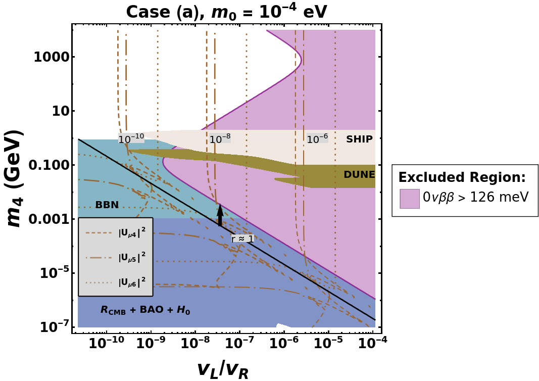
Figure 22: Case (a) with $m_{0}=10^{-4}$ eV.

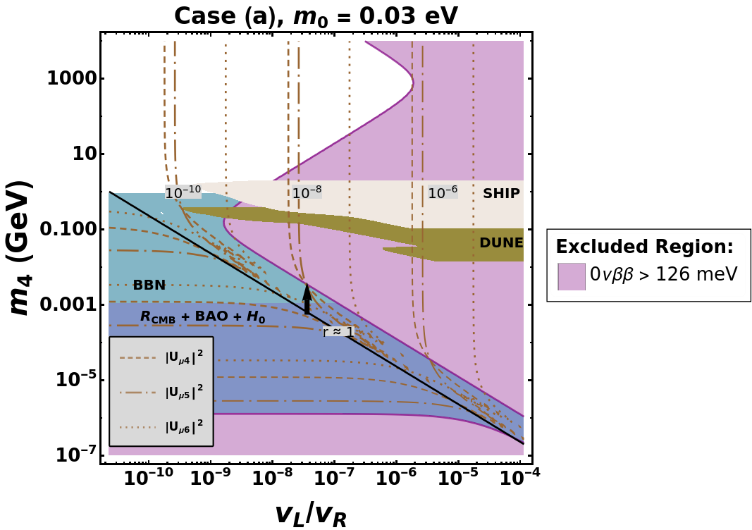
Figure 23: Case (a) with $m_{0}=0.03$ eV.

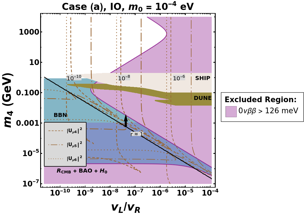
Figure 24: Case (a) but for IO and $m_{0}=10^{-4}$ eV.

C.3 $U_{L}$ and $\phi_{i}$

References

- (1) I. Esteban, M. C. Gonzalez-Garcia, M. Maltoni, T. Schwetz, and A. Zhou, The fate of hints: updated global analysis of three-flavor neutrino oscillations, JHEP 09 (2020) 178, [arXiv:2007.14792].
- (2) K. J. Kelly, P. A. N. Machado, S. J. Parke, Y. F. Perez-Gonzalez, and R. Z. Funchal, Neutrino mass ordering in light of recent data, Phys. Rev. D 103 (2021), no. 1 013004, [arXiv:2007.08526].
- (3) KATRIN Collaboration, M. Aker et al., Direct neutrino-mass measurement with sub-electronvolt sensitivity, Nature Phys. 18 (2022), no. 2 160–166, [arXiv:2105.08533].
- (4) Planck Collaboration, N. Aghanim et al., Planck 2018 results. VI. Cosmological parameters, Astron. Astrophys. 641 (2020) A6, [arXiv:1807.06209]. [Erratum: Astron.Astrophys. 652, C4 (2021)].
- (5) MEG II Collaboration, A. M. Baldini et al., The design of the MEG II experiment, Eur. Phys. J. C 78 (2018), no. 5 380, [arXiv:1801.04688].
- (6) A. Blondel et al., Research Proposal for an Experiment to Search for the Decay , arXiv:1301.6113.
- (7) Mu3e Collaboration, N. Berger, The Mu3e Experiment, Nucl. Phys. B Proc. Suppl. 248-250 (2014) 35–40.
- (8) COMET Collaboration, R. Abramishvili et al., COMET Phase-I Technical Design Report, PTEP 2020 (2020), no. 3 033C01, [arXiv:1812.09018].
- (9) Mu2e Collaboration, L. Bartoszek et al., Mu2e Technical Design Report, arXiv:1501.05241.
- (10) M. Agostini, G. Benato, and J. Detwiler, Discovery probability of next-generation neutrinoless double- decay experiments, Phys. Rev. D 96 (2017), no. 5 053001, [arXiv:1705.02996].
- (11) S. Weinberg, Baryon and Lepton Nonconserving Processes, Phys. Rev. Lett. 43 (1979) 1566–1570.
- (12) P. Minkowski, at a Rate of One Out of Muon Decays?, Phys. Lett. B 67 (1977) 421–428.
- (13) M. Gell-Mann, P. Ramond, and R. Slansky, Complex Spinors and Unified Theories, Conf. Proc. C 790927 (1979) 315–321, [arXiv:1306.4669].
- (14) T. Yanagida, Horizontal gauge symmetry and masses of neutrinos, Conf. Proc. C 7902131 (1979) 95–99.
- (15) R. N. Mohapatra and G. Senjanovic, Neutrino Mass and Spontaneous Parity Nonconservation, Phys. Rev. Lett. 44 (1980) 912.
- (16) J. Schechter and J. W. F. Valle, Neutrino Masses in SU(2) x U(1) Theories, Phys. Rev. D 22 (1980) 2227.
- (17) R. Foot, H. Lew, X. G. He, and G. C. Joshi, Seesaw Neutrino Masses Induced by a Triplet of Leptons, Z. Phys. C 44 (1989) 441.
- (18) J. C. Pati and A. Salam, Lepton Number as the Fourth Color, Phys. Rev. D 10 (1974) 275–289. [Erratum: Phys.Rev.D 11, 703–703 (1975)].
- (19) R. N. Mohapatra and J. C. Pati, A Natural Left-Right Symmetry, Phys. Rev. D 11 (1975) 2558.
- (20) G. Senjanovic and R. N. Mohapatra, Exact Left-Right Symmetry and Spontaneous Violation of Parity, Phys. Rev. D 12 (1975) 1502.
- (21) R. N. Mohapatra and G. Senjanovic, Neutrino Masses and Mixings in Gauge Models with Spontaneous Parity Violation, Phys. Rev. D 23 (1981) 165.
- (22) J. Barry and W. Rodejohann, Lepton number and flavour violation in TeV-scale left-right symmetric theories with large left-right mixing, JHEP 09 (2013) 153, [arXiv:1303.6324].
- (23) P. S. Bhupal Dev, S. Goswami, and M. Mitra, TeV Scale Left-Right Symmetry and Large Mixing Effects in Neutrinoless Double Beta Decay, Phys. Rev. D 91 (2015), no. 11 113004, [arXiv:1405.1399].
- (24) G. Bambhaniya, P. S. B. Dev, S. Goswami, and M. Mitra, The Scalar Triplet Contribution to Lepton Flavour Violation and Neutrinoless Double Beta Decay in Left-Right Symmetric Model, JHEP 04 (2016) 046, [arXiv:1512.00440].
- (25) S. Goswami and K. N. Vishnudath, Low energy constraints from absolute neutrino mass observables and lepton flavor violation in left-right symmetric model, Phys. Rev. D 103 (2021), no. 5 055016, [arXiv:2011.06314].
- (26) V. Tello, M. Nemevsek, F. Nesti, G. Senjanovic, and F. Vissani, Left-Right Symmetry: from LHC to Neutrinoless Double Beta Decay, Phys. Rev. Lett. 106 (2011) 151801, [arXiv:1011.3522].
- (27) G. Li, M. Ramsey-Musolf, and J. C. Vasquez, Left-Right Symmetry and Leading Contributions to Neutrinoless Double Beta Decay, Phys. Rev. Lett. 126 (2021), no. 15 151801, [arXiv:2009.01257].
- (28) N. G. Deshpande, J. F. Gunion, B. Kayser, and F. I. Olness, Left-right symmetric electroweak models with triplet Higgs, Phys. Rev. D 44 (1991) 837–858.
- (29) J. A. Casas and A. Ibarra, Oscillating neutrinos and , Nucl. Phys. B 618 (2001) 171–204, [hep-ph/0103065].
- (30) M. Nemevsek, G. Senjanovic, and V. Tello, Connecting Dirac and Majorana Neutrino Mass Matrices in the Minimal Left-Right Symmetric Model, Phys. Rev. Lett. 110 (2013), no. 15 151802, [arXiv:1211.2837].
- (31) G. Senjanović and V. Tello, Probing Seesaw with Parity Restoration, Phys. Rev. Lett. 119 (2017), no. 20 201803, [arXiv:1612.05503].
- (32) CDF Collaboration, T. Aaltonen et al., High-precision measurement of the W boson mass with the CDF II detector, Science 376 (2022), no. 6589 170–176.
- (33) F. del Aguila, J. de Blas, and M. Perez-Victoria, Electroweak Limits on General New Vector Bosons, JHEP 09 (2010) 033, [arXiv:1005.3998].
- (34) M. Lindner, F. S. Queiroz, and W. Rodejohann, Dilepton bounds on left–right symmetry at the LHC run II and neutrinoless double beta decay, Phys. Lett. B 762 (2016) 190–195, [arXiv:1604.07419].
- (35) CMS Collaboration, A. Tumasyan et al., Search for a right-handed W boson and a heavy neutrino in proton-proton collisions at = 13 TeV, arXiv:2112.03949.
- (36) A. Maiezza, G. Senjanović, and J. C. Vasquez, Higgs sector of the minimal left-right symmetric theory, Phys. Rev. D 95 (2017), no. 9 095004, [arXiv:1612.09146].
- (37) S. Bertolini, A. Maiezza, and F. Nesti, Kaon CP violation and neutron EDM in the minimal left-right symmetric model, Phys. Rev. D 101 (2020), no. 3 035036, [arXiv:1911.09472].
- (38) W. Dekens, L. Andreoli, J. de Vries, E. Mereghetti, and F. Oosterhof, A low-energy perspective on the minimal left-right symmetric model, JHEP 11 (2021) 127, [arXiv:2107.10852].
- (39) Y. Zhang, H. An, X. Ji, and R. N. Mohapatra, General CP Violation in Minimal Left-Right Symmetric Model and Constraints on the Right-Handed Scale, Nucl. Phys. B 802 (2008) 247–279, [arXiv:0712.4218].
- (40) ATLAS Collaboration, M. Aaboud et al., Search for doubly charged Higgs boson production in multi-lepton final states with the ATLAS detector using proton–proton collisions at , Eur. Phys. J. C 78 (2018), no. 3 199, [arXiv:1710.09748].
- (41) G. C. Branco and G. Senjanovic, The Question of Neutrino Mass, Phys. Rev. D 18 (1978) 1621.
- (42) W. R. Inc., “Mathematica, Version 13.0.0.” Champaign, IL, 2021.
- (43) V. Shtabovenko, R. Mertig, and F. Orellana, New developments in FeynCalc 9.0, Computer Physics Communications 207 (oct, 2016) 432–444.
- (44) V. Shtabovenko, R. Mertig, and F. Orellana, FeynCalc 9.3: New features and improvements, Computer Physics Communications 256 (nov, 2020) 107478.
- (45) R. Mertig, M. Böhm, and A. Denner, Feyn calc - computer-algebraic calculation of feynman amplitudes, Computer Physics Communications 64 (1991), no. 3 345–359.
- (46) H. H. Patel, Package-x: A mathematica package for the analytic calculation of one-loop integrals, Computer Physics Communications 197 (2015) 276–290.
- (47) JUNO Collaboration, JUNO physics and detector, Prog. Part. Nucl. Phys. 123 (2022) 103927.
- (48) H. Nunokawa, S. J. Parke, and R. Zukanovich Funchal, Another possible way to determine the neutrino mass hierarchy, Phys. Rev. D 72 (2005) 013009, [hep-ph/0503283].
- (49) JUNO Collaboration, A. Abusleme et al., Sub-percent Precision Measurement of Neutrino Oscillation Parameters with JUNO, arXiv:2204.13249.
- (50) D. V. Forero, S. J. Parke, C. A. Ternes, and R. Z. Funchal, JUNO’s prospects for determining the neutrino mass ordering, Phys. Rev. D 104 (2021), no. 11 113004, [arXiv:2107.12410].
- (51) DUNE Collaboration, B. Abi et al., Long-baseline neutrino oscillation physics potential of the DUNE experiment, Eur. Phys. J. C 80 (2020), no. 10 978, [arXiv:2006.16043].
- (52) Hyper-Kamiokande Proto Collaboration, Y. Kudenko, Hyper-Kamiokande, JINST 15 (2020), no. 07 C07029, [arXiv:2005.13641].
- (53) S. Antusch, C. Biggio, E. Fernandez-Martinez, M. B. Gavela, and J. Lopez-Pavon, Unitarity of the Leptonic Mixing Matrix, JHEP 10 (2006) 084, [hep-ph/0607020].
- (54) E. Fernandez-Martinez, M. B. Gavela, J. Lopez-Pavon, and O. Yasuda, CP-violation from non-unitary leptonic mixing, Phys. Lett. B 649 (2007) 427–435, [hep-ph/0703098].
- (55) S. Goswami and T. Ota, Testing non-unitarity of neutrino mixing matrices at neutrino factories, Phys. Rev. D 78 (2008) 033012, [arXiv:0802.1434].
- (56) S. Antusch, M. Blennow, E. Fernandez-Martinez, and J. Lopez-Pavon, Probing non-unitary mixing and CP-violation at a Neutrino Factory, Phys. Rev. D 80 (2009) 033002, [arXiv:0903.3986].
- (57) F. J. Escrihuela, D. V. Forero, O. G. Miranda, M. Tortola, and J. W. F. Valle, On the description of nonunitary neutrino mixing, Phys. Rev. D 92 (2015), no. 5 053009, [arXiv:1503.08879]. [Erratum: Phys.Rev.D 93, 119905 (2016)].
- (58) S. Parke and M. Ross-Lonergan, Unitarity and the three flavor neutrino mixing matrix, Phys. Rev. D 93 (2016), no. 11 113009, [arXiv:1508.05095].
- (59) D. Dutta and P. Ghoshal, Probing CP violation with T2K, NOA and DUNE in the presence of non-unitarity, JHEP 09 (2016) 110, [arXiv:1607.02500].
- (60) C. S. Fong, H. Minakata, and H. Nunokawa, A framework for testing leptonic unitarity by neutrino oscillation experiments, JHEP 02 (2017) 114, [arXiv:1609.08623].
- (61) S.-F. Ge, P. Pasquini, M. Tortola, and J. W. F. Valle, Measuring the leptonic CP phase in neutrino oscillations with nonunitary mixing, Phys. Rev. D 95 (2017), no. 3 033005, [arXiv:1605.01670].
- (62) M. Blennow, P. Coloma, E. Fernandez-Martinez, J. Hernandez-Garcia, and J. Lopez-Pavon, Non-Unitarity, sterile neutrinos, and Non-Standard neutrino Interactions, JHEP 04 (2017) 153, [arXiv:1609.08637].
- (63) C. S. Fong, H. Minakata, and H. Nunokawa, Non-unitary evolution of neutrinos in matter and the leptonic unitarity test, JHEP 02 (2019) 015, [arXiv:1712.02798].
- (64) I. Martinez-Soler and H. Minakata, Standard versus Non-Standard CP Phases in Neutrino Oscillation in Matter with Non-Unitarity, PTEP 2020 (2020), no. 6 063B01, [arXiv:1806.10152].
- (65) I. Martinez-Soler and H. Minakata, Physics of parameter correlations around the solar-scale enhancement in neutrino theory with unitarity violation, PTEP 2020 (2020), no. 11 113B01, [arXiv:1908.04855].
- (66) S. A. R. Ellis, K. J. Kelly, and S. W. Li, Current and Future Neutrino Oscillation Constraints on Leptonic Unitarity, JHEP 12 (2020) 068, [arXiv:2008.01088].
- (67) A. de Gouvêa and A. Kobach, Global Constraints on a Heavy Neutrino, Phys. Rev. D 93 (2016), no. 3 033005, [arXiv:1511.00683].
- (68) G. Bernardi et al., Search for Neutrino Decay, Phys. Lett. B 166 (1986) 479–483.
- (69) G. Bernardi et al., FURTHER LIMITS ON HEAVY NEUTRINO COUPLINGS, Phys. Lett. B 203 (1988) 332–334.
- (70) DELPHI Collaboration, P. Abreu et al., Search for neutral heavy leptons produced in Z decays, Z. Phys. C 74 (1997) 57–71. [Erratum: Z.Phys.C 75, 580 (1997)].
- (71) Belle Collaboration, D. Liventsev et al., Search for heavy neutrinos at Belle, Phys. Rev. D 87 (2013), no. 7 071102, [arXiv:1301.1105]. [Erratum: Phys.Rev.D 95, 099903 (2017)].
- (72) LHCb Collaboration, R. Aaij et al., Search for Majorana neutrinos in decays, Phys. Rev. Lett. 112 (2014), no. 13 131802, [arXiv:1401.5361].
- (73) ATLAS Collaboration, M. Aaboud et al., Search for heavy Majorana or Dirac neutrinos and right-handed gauge bosons in final states with two charged leptons and two jets at TeV with the ATLAS detector, JHEP 01 (2019) 016, [arXiv:1809.11105].
- (74) CMS Collaboration, A. M. Sirunyan et al., Search for heavy neutral leptons in events with three charged leptons in proton-proton collisions at 13 TeV, Phys. Rev. Lett. 120 (2018), no. 22 221801, [arXiv:1802.02965].
- (75) CMS Collaboration, A. M. Sirunyan et al., Search for heavy Majorana neutrinos in same-sign dilepton channels in proton-proton collisions at TeV, JHEP 01 (2019) 122, [arXiv:1806.10905].
- (76) ATLAS Collaboration, G. Aad et al., Search for heavy neutral leptons in decays of bosons produced in 13 TeV collisions using prompt and displaced signatures with the ATLAS detector, JHEP 10 (2019) 265, [arXiv:1905.09787].
- (77) CMS Collaboration, A. Tumasyan et al., Search for long-lived heavy neutral leptons with displaced vertices in proton-proton collisions at =13 TeV, arXiv:2201.05578.
- (78) ArgoNeuT Collaboration, R. Acciarri et al., New Constraints on Tau-Coupled Heavy Neutral Leptons with Masses mN=280–970 MeV, Phys. Rev. Lett. 127 (2021), no. 12 121801, [arXiv:2106.13684].
- (79) FASER Collaboration, A. Ariga et al., FASER’s physics reach for long-lived particles, Phys. Rev. D 99 (2019), no. 9 095011, [arXiv:1811.12522].
- (80) D. Curtin et al., Long-Lived Particles at the Energy Frontier: The MATHUSLA Physics Case, Rept. Prog. Phys. 82 (2019), no. 11 116201, [arXiv:1806.07396].
- (81) P. Ballett, T. Boschi, and S. Pascoli, Heavy Neutral Leptons from low-scale seesaws at the DUNE Near Detector, JHEP 03 (2020) 111, [arXiv:1905.00284].
- (82) M. Drewes and J. Hajer, Heavy Neutrinos in displaced vertex searches at the LHC and HL-LHC, JHEP 02 (2020) 070, [arXiv:1903.06100].
- (83) A. M. Abdullahi et al., The Present and Future Status of Heavy Neutral Leptons, in 2022 Snowmass Summer Study, 3, 2022. arXiv:2203.08039.
- (84) CMB-S4 Collaboration, K. N. Abazajian et al., CMB-S4 Science Book, First Edition, arXiv:1610.02743.
- (85) A. Boyarsky, M. Ovchynnikov, O. Ruchayskiy, and V. Syvolap, Improved big bang nucleosynthesis constraints on heavy neutral leptons, Phys. Rev. D 104 (2021), no. 2 023517, [arXiv:2008.00749].
- (86) N. Sabti, A. Magalich, and A. Filimonova, An Extended Analysis of Heavy Neutral Leptons during Big Bang Nucleosynthesis, JCAP 11 (2020) 056, [arXiv:2006.07387].
- (87) A. Boyarsky, M. Ovchynnikov, N. Sabti, and V. Syvolap, When feebly interacting massive particles decay into neutrinos: The Neff story, Phys. Rev. D 104 (2021), no. 3 035006, [arXiv:2103.09831].
- (88) A. C. Vincent, E. F. Martinez, P. Hernández, M. Lattanzi, and O. Mena, Revisiting cosmological bounds on sterile neutrinos, JCAP 04 (2015) 006, [arXiv:1408.1956].
- (89) M. Drewes, Y. Georis, and J. Klarić, Mapping the Viable Parameter Space for Testable Leptogenesis, Phys. Rev. Lett. 128 (2022), no. 5 051801, [arXiv:2106.16226].
- (90) J. Kotila and F. Iachello, Phase space factors for double- decay, Phys. Rev. C 85 (2012) 034316, [arXiv:1209.5722].
- (91) G. Pantis, F. Simkovic, J. D. Vergados, and A. Faessler, Neutrinoless double beta decay within QRPA with proton - neutron pairing, Phys. Rev. C 53 (1996) 695–707, [nucl-th/9612036].
- (92) J. D. Vergados, The Neutrino Mass and Family, Lepton and Baryon Nonconservation in Gauge Theories, Phys. Rept. 133 (1986) 1.
- (93) M. Mitra, G. Senjanovic, and F. Vissani, Neutrinoless Double Beta Decay and Heavy Sterile Neutrinos, Nucl. Phys. B 856 (2012) 26–73, [arXiv:1108.0004].
- (94) KamLAND-Zen Collaboration, S. Abe et al., First Search for the Majorana Nature of Neutrinos in the Inverted Mass Ordering Region with KamLAND-Zen, arXiv:2203.02139.
- (95) MEG Collaboration, A. M. Baldini et al., Search for the lepton flavour violating decay with the full dataset of the MEG experiment, Eur. Phys. J. C 76 (2016), no. 8 434, [arXiv:1605.05081].
- (96) A. M. Baldini et al., MEG Upgrade Proposal, arXiv:1301.7225.
- (97) Y. Kuno and Y. Okada, Muon decay and physics beyond the standard model, Rev. Mod. Phys. 73 (2001) 151–202, [hep-ph/9909265].
- (98) C. Cornella, P. Paradisi, and O. Sumensari, Hunting for ALPs with Lepton Flavor Violation, JHEP 01 (2020) 158, [arXiv:1911.06279].
- (99) SINDRUM Collaboration, U. Bellgardt et al., Search for the Decay mu+ — e+ e+ e-, Nucl. Phys. B 299 (1988) 1–6.
- (100) Mu3e Collaboration, K. Arndt et al., Technical design of the phase I Mu3e experiment, Nucl. Instrum. Meth. A 1014 (2021) 165679, [arXiv:2009.11690].
- (101) SINDRUM II Collaboration, C. Dohmen et al., Test of lepton flavor conservation in mu — e conversion on titanium, Phys. Lett. B 317 (1993) 631–636.
- (102) SINDRUM II Collaboration, W. H. Bertl et al., A Search for muon to electron conversion in muonic gold, Eur. Phys. J. C 47 (2006) 337–346.
- (103) SINDRUM II Collaboration, W. Honecker et al., Improved limit on the branching ratio of mu — e conversion on lead, Phys. Rev. Lett. 76 (1996) 200–203.
- (104) R. Kitano, M. Koike, and Y. Okada, Detailed calculation of lepton flavor violating muon electron conversion rate for various nuclei, Phys. Rev. D 66 (2002) 096002, [hep-ph/0203110]. [Erratum: Phys.Rev.D 76, 059902 (2007)].
- (105) T. Aoyama et al., The anomalous magnetic moment of the muon in the Standard Model, Phys. Rept. 887 (2020) 1–166, [arXiv:2006.04822].
- (106) Muon g-2 Collaboration, B. Abi et al., Measurement of the Positive Muon Anomalous Magnetic Moment to 0.46 ppm, Phys. Rev. Lett. 126 (2021), no. 14 141801, [arXiv:2104.03281].
- (107) ACME Collaboration, V. Andreev et al., Improved limit on the electric dipole moment of the electron, Nature 562 (2018), no. 7727 355–360.
- (108) NL-eEDM Collaboration, P. Aggarwal et al., Measuring the electric dipole moment of the electron in BaF, Eur. Phys. J. D 72 (2018), no. 11 197, [arXiv:1804.10012].
- (109) N. J. Fitch, J. Lim, E. A. Hinds, B. E. Sauer, and M. R. Tarbutt, Methods for measuring the electron’s electric dipole moment using ultracold YbF molecules, Quantum Sci. Technol. 6 (2021), no. 1 014006, [arXiv:2009.00346].
- (110) Muon (g-2) Collaboration, G. W. Bennett et al., An Improved Limit on the Muon Electric Dipole Moment, Phys. Rev. D 80 (2009) 052008, [arXiv:0811.1207].
- (111) Muon g-2 Collaboration, R. Chislett, The muon EDM in the g-2 experiment at Fermilab, EPJ Web Conf. 118 (2016) 01005.
- (112) M. Abe et al., A New Approach for Measuring the Muon Anomalous Magnetic Moment and Electric Dipole Moment, PTEP 2019 (2019), no. 5 053C02, [arXiv:1901.03047].
- (113) A. Adelmann et al., Search for a muon EDM using the frozen-spin technique, arXiv:2102.08838.
- (114) M. Sakurai et al., muEDM: Towards a search for the muon electric dipole moment at PSI using the frozen-spin technique, in 24th International Symposium on Spin Physics, 1, 2022. arXiv:2201.06561.
- (115) F. J. M. Farley, K. Jungmann, J. P. Miller, W. M. Morse, Y. F. Orlov, B. L. Roberts, Y. K. Semertzidis, A. Silenko, and E. J. Stephenson, A New method of measuring electric dipole moments in storage rings, Phys. Rev. Lett. 93 (2004) 052001, [hep-ex/0307006].
- (116) Particle Data Group Collaboration, P. A. Zyla et al., Review of Particle Physics, PTEP 2020 (2020), no. 8 083C01.
- (117) M. E. Peskin and T. Takeuchi, A New constraint on a strongly interacting Higgs sector, Phys. Rev. Lett. 65 (1990) 964–967.
- (118) M. E. Peskin and T. Takeuchi, Estimation of oblique electroweak corrections, Phys. Rev. D 46 (1992) 381–409.
- (119) I. Maksymyk, C. P. Burgess, and D. London, Beyond S, T and U, Phys. Rev. D 50 (1994) 529–535, [hep-ph/9306267].
- (120) M. Awramik, M. Czakon, A. Freitas, and G. Weiglein, Precise prediction for the W boson mass in the standard model, Phys. Rev. D 69 (2004) 053006, [hep-ph/0311148].
- (121) M. Blennow, P. Coloma, E. Fernández-Martínez, and M. González-López, Right-handed neutrinos and the CDF II anomaly, arXiv:2204.04559.
- (122) L. Lavoura and L.-F. Li, Making the small oblique parameters large, Phys. Rev. D 49 (1994) 1409–1416, [hep-ph/9309262].
- (123) S. Bertolini, A. Maiezza, and F. Nesti, Present and Future K and B Meson Mixing Constraints on TeV Scale Left-Right Symmetry, Phys. Rev. D 89 (2014), no. 9 095028, [arXiv:1403.7112].
- (124) A. Maiezza, M. Nemevšek, and F. Nesti, Perturbativity and mass scales in the minimal left-right symmetric model, Phys. Rev. D 94 (2016), no. 3 035008, [arXiv:1603.00360].
- (125) R. Balkin, E. Madge, T. Menzo, G. Perez, Y. Soreq, and J. Zupan, On the implications of positive W mass shift, JHEP 05 (2022) 133, [arXiv:2204.05992].
- (126) P. Asadi, C. Cesarotti, K. Fraser, S. Homiller, and A. Parikh, Oblique Lessons from the Mass Measurement at CDF II, arXiv:2204.05283.