Unsupervised Video Domain Adaptation for Action Recognition: A Disentanglement Perspective

Abstract

Unsupervised video domain adaptation is a practical yet challenging task. In this work, for the first time, we tackle it from a disentanglement view. Our key idea is to handle the spatial and temporal domain divergence separately through disentanglement. Specifically, we consider the generation of cross-domain videos from two sets of latent factors, one encoding the static information and another encoding the dynamic information. A Transfer Sequential VAE (TranSVAE) framework is then developed to model such generation. To better serve for adaptation, we propose several objectives to constrain the latent factors. With these constraints, the spatial divergence can be readily removed by disentangling the static domain-specific information out, and the temporal divergence is further reduced from both frame- and video-levels through adversarial learning. Extensive experiments on the UCF-HMDB, Jester, and Epic-Kitchens datasets verify the effectiveness and superiority of TranSVAE compared with several state-of-the-art approaches.

1 Introduction

Over the past decades, unsupervised domain adaptation (UDA) has attracted extensive research attention [41]. Numerous UDA methods have been proposed and successfully applied to various real-world applications, e.g., object recognition [38, 42, 47], semantic segmentation [51, 19, 33, 24], and object detection [3, 15, 45]. However, most of these methods and their applications are limited to the image domain, while much less attention has been devoted to video-based UDA, where the latter is undoubtedly more challenging.

Compared with image-based UDA, the source and target domains also differ temporally in video-based UDA. Images are spatially well-structured data, while videos are sequences of images with both spatial and temporal relations. Existing image-based UDA methods can hardly achieve satisfactory performance on video-based UDA tasks as they fail to consider the temporal dependency of video frames in handling the domain gaps. For instance, in video-based cross-domain action recognition tasks, domain gaps are presented by not only the actions of different persons in different scenarios but also the actions that appear at different timestamps or last at different time lengths.

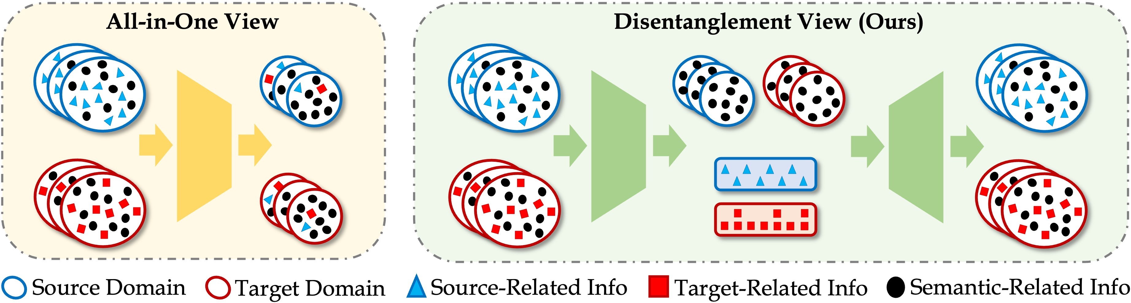
Figure 1: Conceptual comparisons between the traditional all-in-one view and the proposed disentanglement view. Prior works often seek to compress implicit domain information to obtain domain-indistinguishable representations; while in this work, we pursue explicit decouplings of domain-specific information from other information via generative modeling.

Recently, few works have been proposed for video-based UDA. The key idea is to achieve domain alignment by aligning both frame- and video-level features through adversarial learning [7, 26], contrastive learning [37, 31], attention [10], or combination of these mechanisms, e.g., adversarial learning with attention [29, 8]. Though they have advanced video-based UDA, there is still room for improvement. Generally, existing methods follow an all-in-one way, where both spatial and temporal domain divergence are handled together, for adaptation (Fig. 1, $\blacksquare$$\square$). However, cross-domain videos are highly complex data containing diverse mixed-up information, e.g., domain, semantic, and temporal information, which makes the simultaneous elimination of spatial and temporal divergence insufficient. This motivates us to handle the video-based UDA from a disentanglement perspective (Fig. 1, $\blacksquare$$\square$) so that the spatial and temporal divergence can be well handled separately.

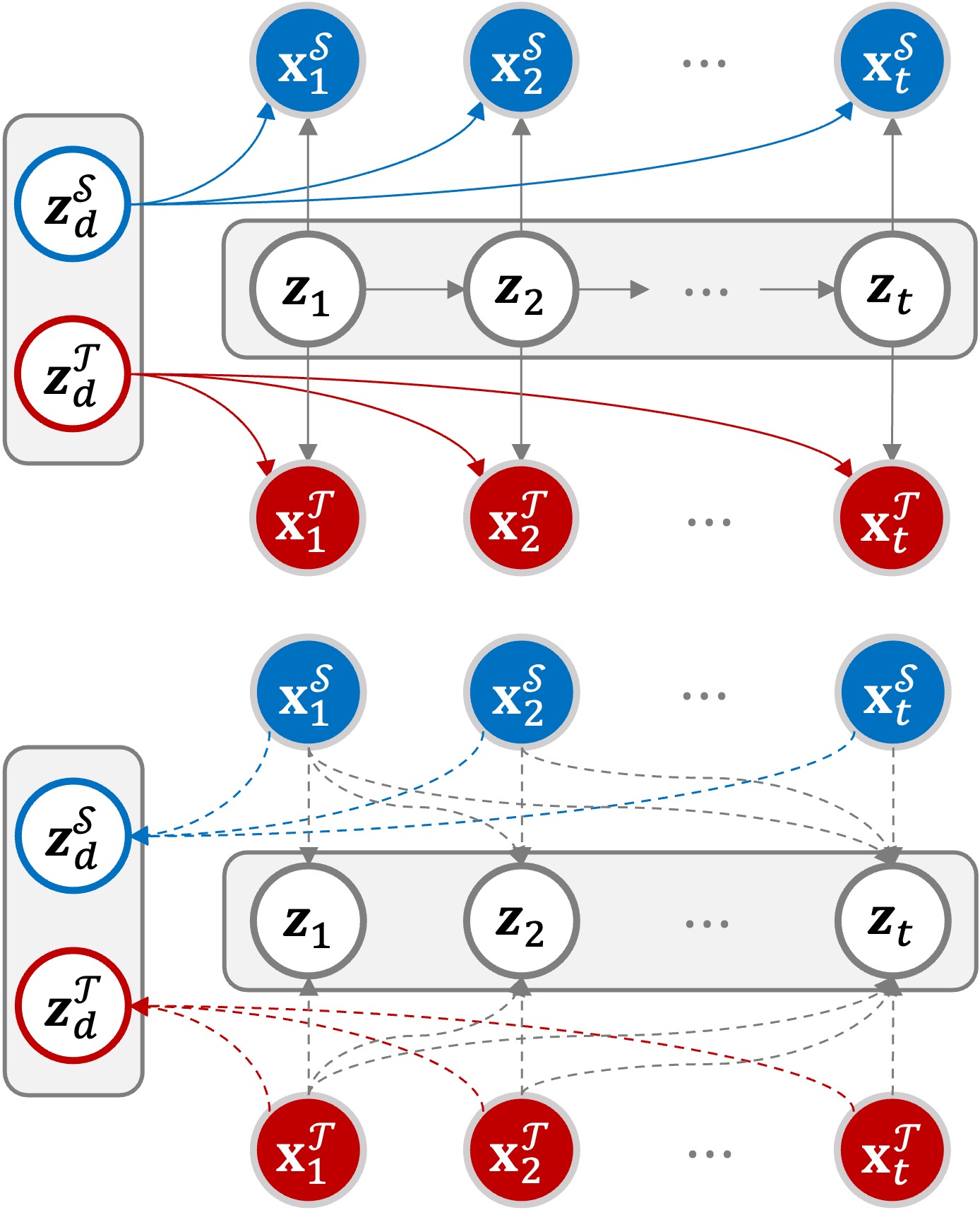
Figure 2: Graphical illustrations of the proposed generative (1st figure) and inference (2nd figure) models for video domain disentanglement.

To achieve this goal, we first consider the generation process of cross-domain videos, as shown in Fig. 2, where a video is generated from two sets of latent factors: one set consists of a sequence of random variables, which are dynamic and incline to encode the semantic information for downstream tasks, e.g., action recognition; another set is static and introduces some domain-related spatial information to the generated video, e.g., style or appearance. Specifically, the blue / red nodes are the observed source / target videos $\mathbf{x}^{\mathcal{S}}$ / $\mathbf{x}^{\mathcal{T}}$, respectively, over $t$ timestamps. Static latent variables $\mathbf{z}_{d}^{\mathcal{S}}$ and $\mathbf{z}_{d}^{\mathcal{T}}$ follow a joint distribution and combining either of them with dynamic latent variables $\mathbf{z}_{t}$ constructs one video data of a domain.

With the above generative model, we develop a Transfer Sequential Variational AutoEncoder (TranSVAE) for video-based UDA. TranSVAE handles the cross-domain divergence in two levels, where the first level removes the spatial divergence by disentangling $\mathbf{z}_{d}$ from $\mathbf{z}_{t}$; while the second level eliminates the temporal divergence of $\mathbf{z}_{t}$. To achieve this, we leverage appropriate constraints to ensure that the disentanglement indeed serves the adaptation purpose. Firstly, we enable a good decoupling of the two sets of latent factors by minimizing their mutual dependence. This encourages these two latent factor sets to be mutually independent. We then consider constraining each latent factor set. For $\mathbf{z}_{d}^{\mathcal{D}}$ with $\mathcal{D}\in\{\mathcal{S},\mathcal{T}\}$, we propose a contrastive triplet loss to make them static and domain-specific. This makes us readily handle spatial divergence by disentangling $\mathbf{z}_{d}^{\mathcal{D}}$ out. For $\mathbf{z}_{t}$, we propose to align them across domains at both frame and video levels through adversarial learning so as to further eliminate the temporal divergence. Meanwhile, as downstream tasks use $\mathbf{z}_{t}$ as input, we also add the task-specific supervision on $\mathbf{z}_{t}$ extracted from source data (w/ ground-truth).

To the best of our knowledge, this is the first work that tackles the challenging video-based UDA from a domain disentanglement view. We conduct extensive experiments on popular benchmarks (UCF-HMDB, Jester, Epic-Kitchens) and the results show that TranSVAE consistently outperforms previous state-of-the-art methods by large margins. We also conduct comprehensive ablation studies and disentanglement analyses to verify the effectiveness of the latent factor decoupling. The main contribution of the paper is summarized as follows:

• We provide a generative perspective on solving video-based UDA problems. We develop a generative graphical model for the cross-domain video generation process and propose to utilize the sequential VAE as the base generative model.

• Based on the above generative view, we propose a TranSVAE framework for video-based UDA. By developing four constraints on the latent factors to enable disentanglement to benefit adaptation, the proposed framework is capable of handling the cross-domain divergence from both spatial and temporal levels.

• We conduct extensive experiments on several benchmark datasets to verify the effectiveness of TranSVAE. A comprehensive ablation study also demonstrates the positive effect of each loss term on video domain adaptation.

2 Related Work

Unsupervised Video Domain Adaptation. Despite the great progress in image-based UDA, only a few methods have recently attempted video-based UDA. In [7], a temporal attentive adversarial adaptation network (TA³N) is proposed to integrate a temporal relation module for temporal alignment. Choi et al. [10] proposed a SAVA method using self-supervised clip order prediction and clip attention-based alignment. Based on a cross-domain co-attention mechanism, the temporal co-attention network TCoN [29] focused on common key frames across domains for better alignment. Luo et al. [26] pay more attention to the domain-agnostic classifier by using a network topology of the bipartite graph to model the cross-domain correlations. Instead of using adversarial learning, Sahoo et al. [31] developed an end-to-end temporal contrastive learning framework named CoMix with background mixing and target pseudo-labels. Recently, Chen et al. [8] learned multiple domain discriminators for multi-level temporal attentive features to achieve better alignment, while Turrisi et al. [37] exploited two-headed deep architecture to learn a more robust target classifier by the combination of cross-entropy and contrastive losses. Although these approaches have advanced video-based UDA tasks, they all adopted to align features with diverse information mixed up from a compression perspective, which leaves room for further improvements.

Multi-Modal Video Adaptation. Most recently, there are also a few works integrating multiple modality data for video-based UDA. Although we only use the single modality RGB features, we still discuss this multi-modal research line for a complete literature review. The very first work exploring the multi-modal nature of videos for UDA is MM-SADA [28], where the correspondence of multiple modalities was exploited as a self-supervised alignment in addition to adversarial alignment. A later work, spatial-temporal contrastive domain adaptation (STCDA) [34], utilized a video-based contrastive alignment as the multi-modal domain metric to measure the video-level discrepancy across domains. [18] proposed cross-modal and cross-domain contrastive losses to handle feature spaces across modalities and domains. [43] leveraged both cross-modal complementary and cross-modal consensus to learn the most transferable features through a CIA framework. In [12], the authors proposed to generate noisy pseudo-labels for the target domain data using the source pre-trained model and select the clean samples in order to increase the quality of the pseudo-labels. Lin et al. [23] developed a cycle-based approach that alternates between spatial and spatiotemporal learning with knowledge transfer. Generally, all the above methods utilize the flow as the auxiliary modality input. Recently, there are also methods exploring other modalities, for instance, A3R [48] with audios and MixDANN [44] with wild data. It is worth noting that the proposed TranSVAE – although only uses single modality RGB features – surprisingly achieves better UDA performance compared with most current state-of-the-art multi-modal methods, which highlights our superiority.

Disentanglement. Feature disentanglement is a wide and hot research topic. We only focus on works that are closely related to ours. In the image domain, some works consider adaptation from a generative view. [4] learned a disentangled semantic representation across domains. A similar idea is then applied to graph domain adaptation [5] and domain generalization [16]. [13] proposed a novel informative feature disentanglement, equipped with the adversarial network or the metric discrepancy model. Another disentanglement-related topic is sequential data generation. To generate videos, existing works [22, 50, 1] extended VAE to a recurrent form with different recursive structures. In this paper, we present a VAE-based structure to generate cross-domain videos. We aim at tackling video-based UDA from a new perspective: sequential domain disentanglement and transfer.

3 Technical Approach

Formally, for a typical video-based UDA problem, we have a source domain $\mathcal{S}$ and a target domain $\mathcal{T}$. Domain $\mathcal{S}$ contains sufficient labeled data, denoted as $\{(\mathbf{V}_{i}^{\mathcal{S}},y_{i}^{\mathcal{S}})\}_{i=1}^{N_{\mathcal{S}}}$, where $\mathbf{V}_{i}^{\mathcal{S}}$ is a video sequence and $y_{i}^{\mathcal{S}}$ is the class label. Domain $\mathcal{T}$ consists of unlabeled data, denoted as $\{\mathbf{V}_{i}^{\mathcal{T}}\}_{i=1}^{N_{\mathcal{T}}}$. For a sequence $\mathbf{V}_{i}^{\mathcal{D}}$ from domain $\mathcal{D}\in\{\mathcal{S},\mathcal{T}\}$, it contains $T$ frames $\{\mathbf{x}_{i\_1}^{\mathcal{D}},...,\mathbf{x}_{i\_T}^{\mathcal{D}}\}$ in total. We further denote $N=N^{\mathcal{S}}+N^{\mathcal{T}}$. Domains $\mathcal{S}$ and $\mathcal{T}$ are of different distributions but share the same label space. The objective is to utilize both $\{(\mathbf{V}_{i}^{\mathcal{S}},y_{i}^{\mathcal{S}})\}_{i=1}^{N_{\mathcal{S}}}$ and $\{\mathbf{V}_{i}^{\mathcal{T}}\}_{i=1}^{N_{\mathcal{T}}}$ to train a good classifier for domain $\mathcal{T}$. We present a table to list the notations in the Appendix.

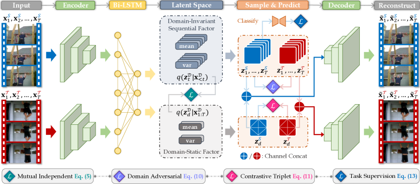
Figure 3: TranSVAE overview. The input videos are fed into an encoder to extract the visual features, followed by an LSTM to explore the temporal information. Two groups of mean and variance networks are then applied to model the posterior of the latent factors, i.e., $q(\mathbf{z}_{t}^{\mathcal{D}}|\mathbf{x}_{<t}^{\mathcal{D}})$ and $q(\mathbf{z}_{d}^{\mathcal{D}}|\mathbf{x}_{1:T}^{\mathcal{D}})$. The new representations $\mathbf{z}_{1}^{\mathcal{D}},...,\mathbf{z}_{T}^{\mathcal{D}}$ and $\mathbf{z}_{d}^{\mathcal{D}}$ are sampled, and then concatenated and passed to a decoder for reconstruction. Four constraints are proposed to regulate the latent factors for adaptation.

Framework Overview. We adopt a VAE-based structure to model the cross-domain video generation process and propose to regulate the two sets of latent factors for adaptation purposes. The reconstruction process is based on the two sets of latent factors, i.e., $\mathbf{z}_{1}^{\mathcal{D}},...,\mathbf{z}_{T}^{\mathcal{D}}$ and $\mathbf{z}_{d}^{\mathcal{D}}$ that are sampled from the posteriors $q(\mathbf{z}_{t}^{\mathcal{D}}|\mathbf{x}_{<t}^{\mathcal{D}})$ and $q(\mathbf{z}_{d}^{\mathcal{D}}|\mathbf{x}_{1:T}^{\mathcal{D}})$, respectively. The overall architecture consists of five segments including the encoder, LSTM, latent spaces, sampling, and decoder, as shown in Fig. 3. The vanilla structure only gives an arbitrary disentanglement of latent factors. To make the disentanglement facilitate adaptation, we carefully constrain the latent factors as follows.

Video Sequence Reconstruction. The overall architecture of TranSVAE follows a VAE-based structure [22, 50, 1] with two sets of latent factors $\mathbf{z}_{1}^{\mathcal{D}},...,\mathbf{z}_{T}^{\mathcal{D}}$ and $\mathbf{z}_{d}^{\mathcal{D}}$. The generative and inference graphical models are presented in Fig. 2. Similar to the conventional VAE, we use a standard Gaussian distribution for static latent factors. For dynamic ones, we use a sequential prior $\mathbf{z}_{t}^{\mathcal{D}}|\mathbf{z}_{<t}^{\mathcal{D}}\sim\mathcal{N}(\boldsymbol{\mu}_{t},diag(\boldsymbol{\sigma}_{t}^{2}))$, that is, the prior distribution of the current dynamic factor is conditioned on the historical dynamic factors. The distribution parameters can be re-parameterized as a recurrent network, e.g., LSTM, with all previous dynamic latent factors as the input. Denoting $\mathbf{Z}^{\mathcal{D}}=\{\mathbf{z}_{1}^{\mathcal{D}},...,\mathbf{z}_{T}^{\mathcal{D}}\}$ for simplification, we then get the prior as follows:

$$p(\mathbf{z}_{d}^{\mathcal{D}},\mathbf{Z}^{\mathcal{D}})=p(\mathbf{z}_{d}^{\mathcal{D}})\prod_{t=1}^{T}p(\mathbf{z}_{t}^{\mathcal{D}}|\mathbf{z}_{<t}^{\mathcal{D}}).$$ (1)

Following Fig. 2 (the 1st subfigure), $\mathbf{x}_{t}^{\mathcal{D}}$ is generated from $\mathbf{z}_{d}^{\mathcal{D}}$ and $\mathbf{z}_{t}^{\mathcal{D}}$, and we thus model $p(\mathbf{x}_{t}^{\mathcal{D}}|\mathbf{z}_{d}^{\mathcal{D}},\mathbf{z}_{t}^{\mathcal{D}})=\mathcal{N}(\boldsymbol{\mu}_{t}^{\prime},diag({\boldsymbol{\sigma}_{t}^{\prime}}^{2}))$. The distribution parameters are re-parameterized by the decoder which can be flexible networks like the deconvolutional neural network. Using $\mathbf{V}^{\mathcal{D}}=\{\mathbf{x}_{1}^{\mathcal{D}},...,\mathbf{x}_{T}^{\mathcal{D}}\}$, the generation can be formulated as follows:

$$p(\mathbf{V}^{\mathcal{D}})=p(\mathbf{z}_{d}^{\mathcal{D}})\prod_{t=1}^{T}p(\mathbf{x}_{t}^{\mathcal{D}}|\mathbf{z}_{d}^{\mathcal{D}},\mathbf{z}_{t}^{\mathcal{D}})p(\mathbf{z}_{t}^{\mathcal{D}}|\mathbf{z}_{<t}^{\mathcal{D}}).$$ (2)

Following Fig. 2 (the 2nd subfigure), we model the posterior distributions of the latent factors as another two Gaussian distributions, i.e., $q(\mathbf{z}_{d}^{\mathcal{D}}|\mathbf{V}^{\mathcal{D}})=\mathcal{N}(\boldsymbol{\mu}_{d},diag(\boldsymbol{\sigma}_{d}^{2}))$ and $q(\mathbf{z}_{t}^{\mathcal{D}}|\mathbf{x}_{<t}^{\mathcal{D}})=\mathcal{N}(\boldsymbol{\mu}_{t}^{\prime\prime},diag({\boldsymbol{\sigma}_{t}^{\prime\prime}}^{2}))$. The parameters of these two distributions are re-parameterized by the encoder, which can be a convolutional or LSTM module. However, the network of the static latent factors uses the whole sequence as the input while that of the dynamic latent factors only uses previous frames. Then the inference can be factorized as:

$$q(\mathbf{z}_{d}^{\mathcal{D}},\mathbf{Z}^{\mathcal{D}}|\mathbf{V}^{\mathcal{D}})=q(\mathbf{z}_{d}^{\mathcal{D}}|\mathbf{V}^{\mathcal{D}})\prod_{t=1}^{T}q(\mathbf{z}_{t}^{\mathcal{D}}|\mathbf{x}_{<t}^{\mathcal{D}}).$$ (3)

Combining the above generation and inference, we obtain the VAE-related objective function as:

$$\begin{split}&\mathcal{L}_{\text{svae}}=\mathbb{E}_{q(\mathbf{z}_{d}^{\mathcal{D}},\mathbf{Z}^{\mathcal{D}}|\mathbf{V}^{\mathcal{D}})}[-\sum_{t=1}^{T}\log p(\mathbf{x}_{t}^{\mathcal{D}}|\mathbf{z}_{d}^{\mathcal{D}},\mathbf{z}_{t}^{\mathcal{D}})]+\\ &\text{KL}(q(\mathbf{z}_{d}^{\mathcal{D}}|\mathbf{V}^{\mathcal{D}})||p(\mathbf{z}_{d}^{\mathcal{D}}))+\sum_{t=1}^{T}\text{KL}(q(\mathbf{z}_{t}^{\mathcal{D}}|\mathbf{x}_{<t}^{\mathcal{D}})||p(\mathbf{z}_{t}^{\mathcal{D}}|\mathbf{z}_{<t}^{\mathcal{D}})),\end{split}$$ (4)

which is a frame-wise negative variational lower bound. Only using the above vanilla VAE-based loss cannot guarantee that the disentanglement serves for adaptation, and thus we propose additional constraints on the two sets of latent factors.

Mutual Dependence Minimization (Fig. 3, $\blacksquare$$\square$). We first consider explicitly enforcing the two sets of latent factors to be mutually independent. To do so, we introduce the mutual information [2] loss $\mathcal{L}_{\text{mi}}$ to regulate the two sets of latent factors. Thus, we obtain:

$$\mathcal{L}_{\text{mi}}(\mathbf{z}_{d}^{\mathcal{D}},\mathbf{Z}^{\mathcal{D}})=\sum_{t=1}^{T}\text{KL}\left(q(\mathbf{z}_{d}^{\mathcal{D}},\mathbf{z}_{t}^{\mathcal{D}})||q(\mathbf{z}_{d}^{\mathcal{D}})q(\mathbf{z}_{t}^{\mathcal{D}})\right)=\sum_{t=1}^{T}[H(\mathbf{z}_{d}^{\mathcal{D}})+H(\mathbf{z}_{t}^{\mathcal{D}})-H(\mathbf{z}_{d}^{\mathcal{D}},\mathbf{z}_{t}^{\mathcal{D}})].$$ (5)

To calculate Eq. (5), we need to estimate the densities of $\mathbf{z}_{d}^{\mathcal{D}},\mathbf{z}_{t}^{\mathcal{D}}$ and $(\mathbf{z}_{d}^{\mathcal{D}},\mathbf{z}_{t}^{\mathcal{D}})$. Following the non-parametric way in [9], we use the mini-batch weighted sampling as follows:

$$H(\mathbf{z})=-\mathbb{E}_{q(\mathbf{z})}[\log q(\mathbf{z})]\approx-\log\frac{1}{M}\sum_{i=1}^{M}[\log\frac{1}{MN}\sum_{j=1}^{M}q\left(\mathbf{z}(\mathbf{x}_{i})|\mathbf{x}_{j}\right)],$$ (6)

where $\mathbf{z}$ is $\mathbf{z}_{d}^{\mathcal{D}},\mathbf{z}_{t}^{\mathcal{D}}$ or $(\mathbf{z}_{d}^{\mathcal{D}},\mathbf{z}_{t}^{\mathcal{D}})$, $N$ denotes the data size and $M$ is the mini-batch size.

Domain Specificity & Static Consistency (Fig. 3, $\blacksquare$$\square$). A characteristic of the domain specificity, e.g., the video style or the objective appearance, is its static consistency over dynamic frames. With this observation, we enable the static and domain-specific latent factors so that we can remove the spatial divergence by disentangling them out. Mathematically, we hope that $\mathbf{z}_{d}^{\mathcal{D}}$ does not change a lot when $\mathbf{z}_{t}^{\mathcal{D}}$ varies over time. To achieve this, given a sequence, we randomly shuffle the temporal order of frames to form a new sequence. The static latent factors disentangled from the original sequence and the shuffled sequence should be ideally equal or be very close at least. This motivates us to minimize the distance between these two static factors. Meanwhile, to further enhance the domain specificity, we enforce the dynamic latent factors from different domains to have a large distance. To this end, we propose the following contrastive triplet loss:

$$\mathcal{L}_{\text{ctc}}=\max\left(D(\mathbf{z}_{d}^{\mathcal{D}^{+}},\widetilde{\mathbf{z}}_{d}^{\mathcal{D}^{+}})-D(\mathbf{z}_{d}^{\mathcal{D}^{+}},\mathbf{z}_{d}^{\mathcal{D}^{-}})+\mathbf{m},0\right),$$ (7)

where $D(\cdot,\cdot)$ is Euclidean distance, $\mathbf{m}$ is a margin set to $1$ in the experiments, $\mathbf{z}_{d}^{\mathcal{D}^{+}}$, $\widetilde{\mathbf{z}}_{d}^{\mathcal{D}^{+}}$, and $\mathbf{z}_{d}^{\mathcal{D}^{-}}$ are static latent factors of the anchor sequence from domain ${\mathcal{D}^{+}}$, the shuffled sequence, and a randomly selected sequence from domain ${\mathcal{D}^{-}}$, respectively. ${\mathcal{D}^{+}}$ and ${\mathcal{D}^{-}}$ represent two different domains.

Domain Temporal Alignment (Fig. 3, $\blacksquare$$\square$). We now consider to reduce the temporal divergence of the dynamic latent factors. There are several ways to achieve this, and in this paper, we take advantage of the most popular adversarial-based idea [14]. Specifically, we build a domain classifier to discriminate whether the data is from $\mathcal{S}$ or $\mathcal{T}$. When back-propagating the gradients, a gradient reversal layer (GRL) is adopted to invert the gradients. Like existing video-based UDA methods, we also conduct both frame-level and video-level alignments. Moreover, as TA³N [7] does, we exploit the temporal relation network (TRN) [49] to discover the temporal relations among different frames, and then aggregate all the temporal relation features into the final video-level features. This enables another level of alignment on the temporal relation features. Thus, we have:

$$\mathcal{L}_{f}=\frac{1}{N}\sum_{i=1}^{N}\frac{1}{T}\sum_{t=1}^{T}CE\left[G_{f}(\mathbf{z}_{i\_t}^{\mathcal{D}}),d_{i}\right],$$ (8)

$$\mathcal{L}_{r}=\frac{1}{N}\sum_{i=1}^{N}\frac{1}{T-1}\sum_{n=2}^{T}CE\left[G_{r}\left(TrN_{n}(\mathbf{Z}_{i}^{\mathcal{D}})\right),d_{i}\right],$$ (9)

$$\mathcal{L}_{v}=\frac{1}{N}\sum_{i=1}^{N}CE\left[G_{v}\left(\frac{1}{T-1}\sum_{n=2}^{T}TrN_{n}(\mathbf{Z}_{i}^{\mathcal{D}})\right),d_{i}\right],$$ (10)

where $d_{i}$ is the domain label, $CE$ denotes the cross-entropy loss function, $\mathbf{Z}_{i}^{\mathcal{D}}=\{\mathbf{z}_{i\_1}^{\mathcal{D}},...,\mathbf{z}_{i\_T}^{\mathcal{D}}\}$, $TrN_{i}$ is the $n$-frame temporal relation network, $G_{f}$, $G_{r}$, and $G_{v}$ are the frame feature level, the temporal relation feature level, and the video feature level domain classifiers, respectively. To this end, we obtain the domain adversarial loss by summing up Eqs. (8-10):

$$\mathcal{L}_{\text{adv}}=\mathcal{L}_{f}+\mathcal{L}_{r}+\mathcal{L}_{v}.$$ (11)

We assign equal importance to these three levels of losses to reduce the overhead of the hyperparameter search. To this end, with $\mathcal{L}_{\text{mi}}$, $\mathcal{L}_{\text{ctc}}$, and $\mathcal{L}_{\text{adv}}$, the learned dynamic latent factors are expected to be domain-invariant (the three constraints are interactive and complementary to each other for obtaining the domain-invariant dynamic latent factor), and then can be used for downstream UDA tasks. In this paper, we specifically focus on action recognition as the downstream task.

Task Specific Supervision (Fig. 3, $\blacksquare$$\square$). We further encourage the dynamic latent factors to carry the semantic information. Considering that the source domain has sufficient labels, we accordingly design the task supervision as the regularization imposed on $\mathbf{z}_{t}^{\mathcal{S}}$. This gives us:

$$\mathcal{L}_{\text{cls}}=\frac{1}{N^{\mathcal{S}}}\sum_{i=1}^{N^{\mathcal{S}}}\mathcal{L}\left(\mathcal{F}(\mathbf{Z}_{i}^{\mathcal{S}}),y_{i}^{\mathcal{S}}\right),$$ (12)

where $\mathcal{F}(\cdot)$ is a feature transformer mapping the frame-level features to video-level features, specifically a TRN in this paper, and $\mathcal{L}(\cdot,\cdot)$ is either cross-entropy or mean squared error loss according to the targeted task.

Although the dynamic latent factors are constrained to be domain-invariant, we do not completely rely on source semantics to learn features discriminative for the target domain. We propose to incorporate target pseudo-labels in task-specific supervision. During the training, we use the prediction network obtained in the previous epoch to generate the target pseudo-labels of the unlabelled target training data for the current epoch. However, to increase the reliability of target pseudo-labels, we let the prediction network be trained only on the source supervision for several epochs and then integrate the target pseudo-labels in the following training epochs. Meanwhile, a confidence threshold is set to determine whether to use the target pseudo-labels or not. Thus, we have the final task-specific supervision as follows:

$$\mathcal{L}_{\text{cls}}=\frac{1}{N}\left(\sum_{i=1}^{N^{\mathcal{S}}}\mathcal{L}(\mathcal{F}(\mathbf{Z}_{i}^{\mathcal{S}}),y_{i}^{\mathcal{S}})+\sum_{i=1}^{N^{\mathcal{T}}}\mathcal{L}(\mathcal{F}(\mathbf{Z}_{i}^{\mathcal{T}}),\widetilde{y}_{i}^{\mathcal{T}})\right),$$ (13)

where $\widetilde{y}_{i}^{\mathcal{T}}$ is the pseudo-label of $\mathbf{Z}_{i}^{\mathcal{T}}$.

Summary. To this end, we reach the final objective function of our TranSVAE framework as follows:

$$\mathcal{L}^{\prime}=\mathcal{L}_{\text{svae}}+\lambda_{1}\mathcal{L}_{\text{mi}}+\lambda_{2}\mathcal{L}_{\text{adv}}+\lambda_{3}\mathcal{L}_{\text{ctc}}+\lambda_{4}\mathcal{L}_{\text{cls}},$$ (14)

where $\lambda_{i}$ with $i=1,2,3,4$ denotes the loss balancing weight.

4 Experiments

In this section, we conduct extensive experimental studies on popular video-based UDA benchmarks to verify the effectiveness of the proposed TranSVAE framework.

4.1 Datasets

UCF-HMDB is constructed by collecting the relevant and overlapping action classes from UCF₁₀₁ [35] and HMDB₅₁ [20]. It contains 3,209 videos in total with 1,438 training videos and 571 validation videos from UCF₁₀₁, and 840 training videos and 360 validation videos from HMDB₅₁. This in turn establishes two video-based UDA tasks: $\mathbf{U}\to\mathbf{H}$ and $\mathbf{H}\to\mathbf{U}$.

Jester [27] consists of 148,092 videos of humans performing hand gestures. Pan et al. [29] constructed a large-scale cross-domain benchmark with seven gesture classes, and form a single transfer task $\mathbf{J}_{\mathcal{S}}\to\mathbf{J}_{\mathcal{T}}$, where $\mathbf{J}_{\mathcal{S}}$ and $\mathbf{J}_{\mathcal{T}}$ contain 51,498 and 51,415 video clips, respectively.

Epic-Kitchens [11] is a challenging egocentric dataset consisting of videos capturing daily activities in kitchens. [28] constructs three domains across the eight largest actions. They are $\mathbf{D}_{1}$, $\mathbf{D}_{2}$, and $\mathbf{D}_{3}$ corresponding to P08, P01, and P22 kitchens of the full dataset, resulting in six cross-domain tasks.

Sprites [22] contains sequences of animated cartoon characters with 15 action categories. The appearances of characters are fully controlled by four attributes, i.e., body, top wear, bottom wear, and hair. We construct two domains, $\mathbf{P}_{1}$ and $\mathbf{P}_{2}$. $\mathbf{P}_{1}$ uses the human body with attributes randomly selected from 3 top wears, 4 bottom wears, and 5 hairs, while $\mathbf{P}_{2}$ uses the alien body with attributes randomly selected from 4 top wears, 3 bottom wears, and 5 hairs. The attribute pools are non-overlapping across domains, resulting in completely heterogeneous $\mathbf{P}_{1}$ and $\mathbf{P}_{2}$. Each domain has 900 video sequences, and each sequence is with 8 frames.

4.2 Implementation Details

Architecture. Following the latest works [31, 37], we use I3D [6] as the backbone. However, different from CoMix which jointly trains the backbone, we simply use the pretrained I3D model on Kinetics [17], provided by [6], to extract RGB features. For the first three benchmarks, RGB features are used as the input of TranSVAE. For Sprites, we use the original image as the input, for the purpose of visualizing the reconstruction and disentanglement results. We use the shared encoder and decoder structures across the source and target domains. For RGB feature inputs, the encoder and decoder are fully connected layers. For original image inputs, the encoder and decoder are the convolution and deconvolution layers (from DCGAN [46]), respectively. For the TRN model, we directly use the one provided by [7]. Other details on this aspect are placed in Appendix.

Table 1: UDA performance comparisons on UCF-HMDB.

Method & Year	Backbone	$\mathbf{U}\to\mathbf{H}$	$\mathbf{H}\to\mathbf{U}$	Average $\uparrow$
DANN (JMLR’16)	ResNet-101	$75.28$	$76.36$	$75.82$
JAN (ICML’17)	ResNet-101	$74.72$	$76.69$	$75.71$
AdaBN (PR’18)	ResNet-101	$72.22$	$77.41$	$74.82$
MCD (CVPR’18)	ResNet-101	$73.89$	$79.34$	$76.62$
TA3N (ICCV’19)	ResNet-101	$78.33$	$81.79$	$80.06$
ABG (MM’20)	ResNet-101	$79.17$	$85.11$	$82.14$
TCoN (AAAI’20)	ResNet-101	$87.22$	$89.14$	$88.18$
MA2L-TD (WACV’22)	ResNet-101	$85.00$	$86.59$	$85.80$
Source-only ($\mathcal{S}_{\text{only}}$)	I3D	$80.27$	$88.79$	$84.53$
DANN (JMLR’16)	I3D	$80.83$	$88.09$	$84.46$
ADDA (CVPR’17)	I3D	$79.17$	$88.44$	$83.81$
TA3N (ICCV’19)	I3D	$81.38$	$90.54$	$85.96$
SAVA (ECCV’20)	I3D	$82.22$	$91.24$	$86.73$
CoMix (NeurIPS’21)	I3D	$86.66$	$93.87$	$90.22$
CO2A (WACV’22)	I3D	$87.78$	$95.79$	$91.79$
TranSVAE (Ours)	I3D	$\mathbf{87.78}$	$\mathbf{98.95}$	$\mathbf{93.37}$
Supervised-target ($\mathcal{T}_{\text{sup}}$)	I3D	$95.00$	$96.85$	$95.93$

Configurations. Our TranSVAE is implemented with PyTorch [30]. We use Adam with a weight decay of $1e^{-4}$ as the optimizer. The learning rate is initially set to be $1e^{-3}$ and follows a commonly used decreasing strategy in [14]. The batch size and the learning epoch are uniformly set to be 128 and 1,000, respectively, for all the experiments. We uniformly set 100 epochs of training under only source supervision and involved the target pseudo-labels afterward. Following the common protocol in video-based UDA [37], we perform hyperparameter selection on the validation set. The specific hyperparameters used for each task can be found in the Appendix. NVIDIA A100 GPUs are used for all experiments. Kindly refer to our Appendix for all other details.

Competitors. We compared methods from three lines. We first consider the source-only ($\mathcal{S}_{\text{only}}$) and supervised-target ($\mathcal{T}_{\text{sup}}$) which uses only labeled source data and only labeled target data, respectively. These two baselines serve as the lower and upper bounds for our tasks. Secondly, we consider five popular image-based UDA methods by simply ignoring temporal information, namely DANN [14], JAN [25], ADDA [38], AdaBN [21], and MCD [32]. Lastly and most importantly, we compare recent SoTA video-based UDA methods, including TA³N [7], SAVA [10], TCoN [29], ABG [26], CoMix [31], CO²A [37], and MA²L-TD [8]. All these methods use single modality features. We directly quote numbers reported in published papers whenever possible. There exist recent works conducting video-based UDA using multi-modal data, e.g. RGB + Flow. Although TranSVAE solely uses RGB features, we still take this set of methods into account. Specifically, we consider MM-SADA [28], STCDA [34], CMCD [18], A3R [48], CleanAdapt [12], CycDA [23], MixDANN [44] and CIA [43].

4.3 Comparative Study

Results on UCF-HMDB. Tab. 1 shows comparisons of TranSVAE with baselines and SoTA methods on UCF-HMDB. The best result among all the baselines is highlighted using bold. Overall, methods using the I3D backbone [6] achieve better results than those using ResNet-101. Our TranSVAE consistently outperforms all previous methods. In particular, TranSVAE achieves $93.37\%$ average accuracy, improving the best competitor CO²A [37], with the same I3D backbone [6], by $1.38\%$. Surprisingly, we observe that TranSVAE even yields better results (by a $2.1\%$ improvement) than the supervised-target ($\mathcal{T}_{\text{sup}}$) baseline. This is because the $\mathbf{H}\to\mathbf{U}$ task already has a good performance without adaptation, i.e., $88.79\%$ for the source-only ($\mathcal{S}_{\text{only}}$) baseline, and thus the target pseudo-labels used in TranSVAE are almost correct. By further aligning domains and equivalently augmenting training data, TranSVAE outperforms $\mathcal{T}_{\text{sup}}$ which is only trained with target data.

Table 2: UDA performance comparisons to approaches using multi-modality data as the input.

Task	$\mathcal{S}_{\text{only}}$	MM-SADA	STCDA	CMCD	A3R	CleanAdapt	CycDA	MixDANN	CIA	TranSVAE
$\mathbf{U}\to\mathbf{H}$	$86.1$	$84.2$	$83.1$	$84.7$	/	$\mathbf{89.8}$	$88.1$	$82.2$	$\mathbf{88.3}$	$87.8$ ($\mathbf{+1.7}$)
$\mathbf{H}\to\mathbf{U}$	$92.5$	$91.1$	$92.1$	$92.8$	/	$\mathbf{99.2}$	$98.0$	$92.8$	$94.1$	${99.0}$ ($\mathbf{+6.5}$)
Average $\uparrow$	$89.3$	$87.7$	$87.6$	$88.8$	/	$\mathbf{94.5}$	$93.1$	$87.5$	$91.2$	${93.4}$ ($\mathbf{+4.1}$)
$\mathbf{D}_{1}\to\mathbf{D}_{2}$	$43.2$	$49.5$	$52.0$	$50.3$	$\mathbf{53.2}$	$52.7$	/	$56.0$	${52.5}$	$50.5$ ($\mathbf{+7.3}$)
$\mathbf{D}_{1}\to\mathbf{D}_{3}$	$42.5$	$44.1$	$45.5$	$46.3$	$\mathbf{52.1}$	$47.0$	/	$47.3$	$47.8$	${50.3}$ ($\mathbf{+7.8}$)
$\mathbf{D}_{2}\to\mathbf{D}_{1}$	$43.0$	$48.2$	$49.0$	$49.5$	$\mathbf{51.9}$	$46.2$	/	$50.3$	$49.8$	${50.3}$ ($\mathbf{+7.3}$)
$\mathbf{D}_{2}\to\mathbf{D}_{3}$	$48.0$	$52.7$	$52.5$	$52.0$	$55.5$	$52.7$	/	$52.4$	$53.2$	$\mathbf{58.6}$ ($\mathbf{+10.6}$)
$\mathbf{D}_{3}\to\mathbf{D}_{1}$	$43.0$	$50.9$	$\mathbf{52.6}$	$48.7$	$51.5$	47.8	/	$51.0$	$52.2$	$48.0$ ($\mathbf{+5.0}$)
$\mathbf{D}_{3}\to\mathbf{D}_{2}$	$55.5$	$56.1$	$55.6$	$56.3$	$\mathbf{63.2}$	$54.4$	/	$54.7$	$57.6$	${58.0}$ ($\mathbf{+2.5}$)
Average $\uparrow$	$45.9$	$50.3$	$51.2$	$51.0$	$\mathbf{54.1}$	$50.3$	/	$52.0$	$52.2$	${52.6}$ ($\mathbf{+6.7}$)

Table 3: Comparison results on Jester and Epic-Kitchens.

Task	$\mathcal{S}_{\text{only}}$	DANN	ADDA	TA3N	CoMix	TranSVAE	$\mathcal{T}_{\text{sup}}$
$\mathbf{J}_{\mathcal{S}}\to\mathbf{J}_{\mathcal{T}}$	$51.5$	$55.4$	$52.3$	$55.5$	$64.7$	$\mathbf{66.1}$ ($\mathbf{+14.6}$)	$95.6$
$\mathbf{D}_{1}\to\mathbf{D}_{2}$	$32.8$	$37.7$	$35.4$	$34.2$	$42.9$	$\mathbf{50.5}$ ($\mathbf{+17.7}$)	$64.0$
$\mathbf{D}_{1}\to\mathbf{D}_{3}$	$34.1$	$36.6$	$34.9$	$37.4$	$40.9$	$\mathbf{50.3}$ ($\mathbf{+16.2}$)	$63.7$
$\mathbf{D}_{2}\to\mathbf{D}_{1}$	$35.4$	$38.3$	$36.3$	$40.9$	$38.6$	$\mathbf{50.3}$ ($\mathbf{+14.9}$)	$57.0$
$\mathbf{D}_{2}\to\mathbf{D}_{3}$	$39.1$	$41.9$	$40.8$	$42.8$	$45.2$	$\mathbf{58.6}$ ($\mathbf{+19.5}$)	$63.7$
$\mathbf{D}_{3}\to\mathbf{D}_{1}$	$34.6$	$38.8$	$36.1$	$39.9$	$42.3$	$\mathbf{48.0}$ ($\mathbf{+13.4}$)	$57.0$
$\mathbf{D}_{3}\to\mathbf{D}_{2}$	$35.8$	$42.1$	$41.4$	$44.2$	$49.2$	$\mathbf{58.0}$ ($\mathbf{+22.2}$)	$64.0$
Average $\uparrow$	$35.3$	$39.2$	$37.4$	$39.9$	$43.2$	$\mathbf{52.6}$ ($\mathbf{+17.3}$)	$61.5$

Results on Jester & Epic-Kitchens. Tab. 3 shows the comparison results on the Jester and Epic-Kitchens benchmarks. We can see that our TranSVAE is the clear winner among all the methods on all the tasks. Specifically, TranSVAE achieves a $1.4\%$ improvement and a $9.4\%$ average improvement over the runner-up baseline CoMix [31] on Jester and Epic-Kitchens, respectively. This verifies the superiority of TranSVAE over others in handling video-based UDA. However, we also notice that the accuracy gap between CoMix and $\mathcal{T}_{\text{sup}}$ is still significant on Jester. This is because the large-scale Jester dataset contains highly heterogeneous data across domains, e.g., the source domain contains videos of the rolling hand forward, while the target domain only consists of videos of the rolling hand backward. This leaves much room for improvement in the future.

Compare to Multi-Modal Methods. We further compare with four recent video-based UDA methods that use multi-modalities, e.g. RGB features, and optical flows, although TranSVAE only uses RGB features. Surprisingly, TranSVAE achieves better average results than seven out of eight multi-modal methods and is only worse than CleanAdapt [12] on UCF-HMDB and A3R [48] on Epic-Kitchens. Considering TranSVAE only uses single-modality data, we are confident that there exists great potential for further improvements of TranSVAE with multi-modal data taken into account.

4.4 Property Analysis

Disentanglement Analysis. We analyze the disentanglement effect of TranSVAE on Sprites [22] and show results in Fig. 4. The left subfigure shows the original sequences of the two domains. The “Human" and “Alien" are completely different appearances and the former is casting spells while the latter is slashing. The middle subfigure shows the sequences reconstructed only using $\{\mathbf{z}_{1}^{\mathcal{D}},...,\mathbf{z}_{T}^{\mathcal{D}}\}$. It can be clearly seen that the two sequences keep the same action as the corresponding original ones. However, if we only focus on the appearance characteristics, it is difficult to distinguish the domain to which the sequences belong. This indicates that $\{\mathbf{z}_{1}^{\mathcal{D}},...,\mathbf{z}_{T}^{\mathcal{D}}\}$ are indeed domain-invariant and well encode the semantic information. The right subfigure shows the sequences reconstructed by exchanging $\mathbf{z}_{d}^{\mathcal{D}}$, which results in two sequences with the same actions but exchanged appearance. This verifies that $\mathbf{z}_{d}^{\mathcal{D}}$ is representing the appearance information, which is actually the domain-related information in this example. This property study sufficiently supports that TranSVAE can successfully disentangle the domain information from other information, with the former embedded in $\mathbf{z}_{d}^{\mathcal{D}}$ and the latter embedded in $\{\mathbf{z}_{1}^{\mathcal{D}},...,\mathbf{z}_{T}^{\mathcal{D}}\}$.

Table 4: Comparison results on model complexity.

Methods	Trainable Params	MACs	FLOPs	FPS
TA3N	$7.6880$ M	$18.2318$ G	$36.4636$ G	$0.0134$ s
CoMix	$30.3688$ M	$18.5640$ G	$37.1280$ G	$0.0157$ s
CO2A	$23.6720$ M	$18.1884$ G	$36.3768$ G	$0.0127$ s
TranSVAE	$12.7419$ M	$18.2657$ G	$36.5314$ G	$0.0133$ s

Complexity Analysis. We further conduct complexity analysis on our TranSVAE. Specifically, we compare the number of trainable parameters, multiply-accumulate operations (MACs), floating-point operations (FLOPs), and inference frame-per-second (FPS) with existing baselines including TA³N [7], CO²A [37], and CoMix [31]. All the comparison results are shown in Tab. 4. From the table, we observe that TranSVAE requires less trainable parameters than CO²A and CoMix. Although more trainable parameters are used than TA³N, TranSVAE achieves significant adaptation performance improvement than TA³N (see Tab. 1 and Tab. 3). Moreover, the MACs, FLOPs, and FPS are competitive among different methods. This is reasonable since all these approaches adopt the same I3D backbone.

Ablation Study. We now analyze the effectiveness of each loss term in Eq. (14). We compare with four variants of TranSVAE, each removing one loss term by equivalently setting the weight $\lambda$ to $0$. The ablation results on UCF-HMDB, Jester, and Epic-Kitchens are shown in Tab. 5. As can be seen, removing $\mathcal{L}_{\text{cls}}$ significantly reduces the transfer performance in all the tasks. This is reasonable as $\mathcal{L}_{\text{cls}}$ is used to discover the discriminative features. Removing any of $\mathcal{L}_{\text{adv}}$, $\mathcal{L}_{\text{mi}}$, and $\mathcal{L}_{\text{ctc}}$ leads to an inferior result than the full TranSVAE setup, and removing $\mathcal{L}_{\text{adv}}$ is the most influential. This is because $\mathcal{L}_{\text{adv}}$ is used to explicitly reduce the temporal domain gaps. All these results demonstrate that every proposed loss matters in our framework.

Table 5: Loss separation study on different video-based UDA tasks by dropping each loss sequentially.

$\mathcal{L}_{\text{svae}}$	$\mathcal{L}_{\text{cls}}$	$\mathcal{L}_{\text{adv}}$	$\mathcal{L}_{\text{mi}}$	$\mathcal{L}_{\text{ctc}}$	PL	$\mathbf{U}\to\mathbf{H}$	$\mathbf{H}\to\mathbf{U}$	$\mathbf{J}_{\mathcal{S}}\to\mathbf{J}_{\mathcal{T}}$	$\mathbf{D}_{1}\to\mathbf{D}_{2}$	$\mathbf{D}_{1}\to\mathbf{D}_{3}$	$\mathbf{D}_{2}\to\mathbf{D}_{1}$	$\mathbf{D}_{2}\to\mathbf{D}_{3}$	$\mathbf{D}_{3}\to\mathbf{D}_{1}$	$\mathbf{D}_{3}\to\mathbf{D}_{2}$	Avg.
✓		✓	✓	✓	✓	$18.61$	$26.62$	$22.92$	$34.00$	$30.29$	$33.79$	$30.49$	$28.51$	$34.27$	$28.83$
✓	✓		✓	✓	✓	$83.06$	$93.52$	$48.07$	$40.93$	$43.33$	$43.91$	$51.13$	$41.84$	$52.67$	$55.38$
✓	✓	✓		✓	✓	$85.83$	$93.52$	$65.12$	$46.67$	$48.56$	$49.43$	$55.34$	$45.52$	$54.53$	$60.60$
✓	✓	✓	✓		✓	$83.89$	$95.80$	$64.89$	$48.53$	$48.25$	$48.96$	$54.21$	$45.52$	$55.73$	$60.64$
✓	✓	✓	✓	✓		$87.22$	$94.40$	$64.64$	$49.87$	$48.25$	$49.66$	$56.47$	$47.59$	$55.07$	$61.46$
✓	✓	✓	✓	✓	✓	$\mathbf{87.78}$	$\mathbf{98.95}$	$\mathbf{66.10}$	$\mathbf{50.53}$	$\mathbf{50.31}$	$\mathbf{50.34}$	$\mathbf{58.62}$	$\mathbf{48.04}$	$\mathbf{58.00}$	$\mathbf{63.19}$

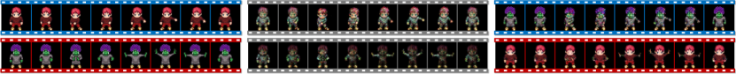
Figure 4: Domain disentanglement and transfer examples. Left: Video sequence inputs for $\mathcal{D}=\mathbf{P}_{1}$ (“Human", $\blacksquare$$\square$) and $\mathcal{D}=\mathbf{P}_{2}$ (“Alien", $\blacksquare$$\square$). Middle: Reconstructed sequences ($\blacksquare$$\square$) with $\mathbf{z}_{1}^{\mathcal{D}},...,\mathbf{z}_{T}^{\mathcal{D}}$. Right: Domain transferred sequences with exchanged $\mathbf{z}_{d}^{\mathcal{D}}$.

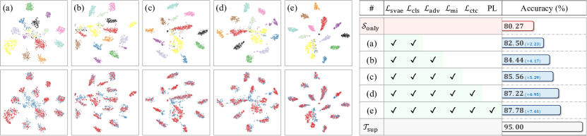
Figure 5: Loss integration studies on $\mathbf{U}\to\mathbf{H}$. Left: The t-SNE plots for class-wise (top row) and domain (bottom row, red source & blue target) features. Right: Ablation results (%) by adding each loss sequentially, i.e., row (a) - row (e).

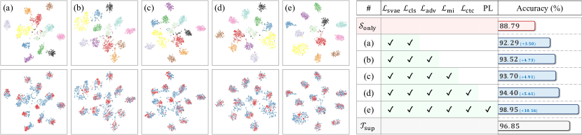
Figure 6: Loss integration studies on $\mathbf{H}\to\mathbf{U}$. Left: The t-SNE plots for class-wise (top row) and domain (bottom row, red source & blue target) features. Right: Ablation results (%) by adding each loss sequentially, i.e., row (a) - row (e).

We further conduct another ablation study by sequentially integrating $\mathcal{L}_{\text{cls}}$, $\mathcal{L}_{\text{adv}}$, $\mathcal{L}_{\text{mi}}$, and $\mathcal{L}_{\text{ctc}}$ into our sequential VAE structure using UCF-HMDB. We use this integration order based on the average positive improvement that a loss brings to TranSVAE as shown in Tab. 5. We also take advantage of t-SNE [39] to visualize the features learned by these different variants. We plot two sets of t-SNE figures, one using the class-wise label and another using the domain label. Fig. 5 and Fig. 6 show the visualization and the quantitative results. As can be seen from the t-SNE feature visualizations, adding a new component improves both the domain and semantic alignments, and the best alignment is achieved when all the components are considered. The quantitative results further show that the transfer performance gradually increases with the sequential integration of the four components, which again verifies the effectiveness of each component in TranSVAE. More ablation study results can be found in the Appendix.

5 Conclusion and Limitation

In this paper, we proposed a TranSVAE framework for video-based UDA tasks. Our key idea is to explicitly disentangle the domain information from other information during the adaptation. We developed a novel sequential VAE structure with two sets of latent factors and proposed four constraints to regulate these factors for adaptation purposes. Note that disentanglement and adaptation are interactive and complementary. All the constraints serve to achieve a good disentanglement effect with the two-level domain divergence minimization. Extensive empirical studies clearly verify that TranSVAE consistently offers performance improvements compared with existing SoTA video-based UDA methods. We also find that TranSVAE outperforms those multi-modal UDA methods, although it only uses single-modality data. Comprehensive property analysis further shows that TranSVAE is an effective and promising method for video-based UDA.

We further discuss the limitations of the TranSVAE framework. These are also promising future directions. Firstly, the empirical evaluation is mainly on the action recognition task. The performance of TranSVAE on other video-related tasks, e.g. video segmentation, is not tested. Secondly, TranSVAE is only evaluated on the typical two-domain transfer scenario. The multi-source transfer case is not considered but is worthy of further study. Thirdly, although TranSVAE exhibits better performance than multi-modal transfer methods, its current version does not consider multi-modal data functionally and structurally. An improved TranSVAE with the capacity of using multi-modal data is expected to further boost the adaptation performance. Fourthly, current empirical evaluations are mainly based on the I3D backbone, more advanced backbones, e.g., [36, 40], are expected to be explored for further improvement. Lastly, TranSVAE handles the spatial divergence by disentangling the static domain-specific latent factors out. However, it may happen that spatial divergence is not completely captured by the static latent factors due to insufficient disentanglement.

Appendix

In this appendix, we supplement the following materials to support the findings and conclusions drawn in the main body of this paper:

• Sec. 6 provides additional implementation details to assist reproductions.

• Sec. 7 contains additional comparative and ablation results of the TranSVAE framework.

• Sec. 8 elaborates on the broader impact of this work.

• Sec. 9 acknowledges the public resources used during the course of this work.

6 Additional Implementation Details

In this section, we provide more implementation details including the I3D feature extraction procedure, the concrete model architecture, and the hyperparameter selection in our proposed TranSVAE framework. We also provide detailed instructions for our live demo.

6.1 Notations

We present Tab. 6 to summarize the notations used in this paper.

6.2 I3D Feature Extractions

We extract the I3D RGB features following the routine described in SAVA [10]. Given a video sequence, $16$ frames along clips are sampled by sliding a temporal window with a temporal stride of $1$. Specifically, for each frame in the video, the temporal window consists of its previous seven frames and the following eight frames. Zero padding is used for the beginning and the end of the video. We then feed the sliding windows to the I3D backbone to extract features, which results in a $1024$-dimensional feature vector for each frame of the video.

6.3 Model Architecture

We now provide the detailed model architecture of our TranSVAE. In Fig. 7, we show the model with the image as the input, where the encoder and decoder are more complex convolutional and deconvolutional layers. For the model with the RGB features as the input, we can simply replace the encoder and decoder with fully connected linear layers. Note that the dimensionality of all the modules shown above is uniformly applied in all the experiments.

6.4 Hyperparameter Selection

There are several hyperparameters used in TranSVAE, including the balancing weights $\lambda_{1}$, $\lambda_{2}$, $\lambda_{3}$, $\lambda_{4}$, the number of the video frames $T$, and the confidence threshold $\eta$ for generating target pseudo-labels. For $\lambda_{1}$ to $\lambda_{4}$, we select from the value set $\{1e^{-3},1e^{-2},1e^{-1},0.5,1,5,10,50,100,1000\}$. For $T$, we select from $\{5,6,7,8,9,10\}$. For $\eta$, we set its value range from $0.9$ to $1.0$ with a step of $0.01$.

We set a high-value range of $\eta$ to ensure a high confidence score on the correctness of the target pseudo-labels. Following the common protocol used in video-based UDA, we conduct an extensive grid search regarding these hyperparameters on the validation set of each transfer task. Tab. 7 summarizes the exact used values of these hyperparameters for the UCF-HMDB [35, 20], Jester [27], and Epic-Kitchens [11] UDA benchmarks. For the Sprites [22] dataset, we do not do a hyperparameter search as the data is quite simple. We simply set $T$ as $8$, which is the original length of the video sequence. The confidence threshold is set to be $0.99$, and $\lambda_{1}$ to $\lambda_{4}$ are all set to be $1$.

Table 6: Summary of notations used in this paper.

Notation	Description
$\mathcal{D}$	Domain
$\mathcal{S}/\mathcal{T}$	Source domain / Target domain
$\mathbf{V}^{\mathcal{D}}$	A video sequence from domain $\mathcal{D}$
$\mathbf{V}^{\mathcal{D}}_{i},y_{i}^{\mathcal{D}}$	The $i$-th video sequence and the corresponding action label of domain $\mathcal{D}$
$\mathbf{x}_{i}^{\mathcal{D}},...,\mathbf{x}_{T}^{\mathcal{D}}$	$T$ frames of images in the video sequence $\mathbf{V}^{\mathcal{D}}$
$\mathbf{z}_{i}^{\mathcal{D}},...,\mathbf{z}_{T}^{\mathcal{D}}$	The dynamic latent factors of the video sequence from domain $\mathcal{D}$
$\mathbf{z}_{d}^{\mathcal{D}}$	The static latent factors of the video sequence from domain $\mathcal{D}$
$\mathbf{x}_{<t}^{\mathcal{D}}$	The input sequence before timestamp $t$
$\mathbf{x}_{1:T}^{\mathcal{D}}$	The full input sequence from $t=1$ to $t=T$.

Table 7: Summary of the best-possible hyperparameter values of the TranSVAE framework for each UDA task in our experiments after an extensive grid search.

Task	Backbone	$T$	$\eta$	$\lambda_{1}$	$\lambda_{2}$	$\lambda_{3}$	$\lambda_{4}$
$\mathbf{U}\to\mathbf{H}$	I3D	$8$	$0.93$	$50$	$1$	$1$	$1$
$\mathbf{H}\to\mathbf{U}$	I3D	$9$	$0.96$	$0.5$	$0.1$	$10$	$1$
$\mathbf{J}_{\mathcal{S}}\to\mathbf{J}_{\mathcal{T}}$	I3D	$6$	$0.95$	$0.001$	$10$	$100$	$10$
$\mathbf{D}_{1}\to\mathbf{D}_{2}$	I3D	$9$	$0.96$	$50$	$10$	$5$	$100$
$\mathbf{D}_{1}\to\mathbf{D}_{3}$	I3D	$10$	$1$	$1$	$0.5$	$0.1$	$100$
$\mathbf{D}_{2}\to\mathbf{D}_{1}$	I3D	$8$	$0.93$	$100$	$10$	$5$	$100$
$\mathbf{D}_{2}\to\mathbf{D}_{3}$	I3D	$10$	$0.91$	$0.5$	$10$	$50$	$100$
$\mathbf{D}_{3}\to\mathbf{D}_{1}$	I3D	$8$	$0.91$	$100$	$10$	$50$	$100$
$\mathbf{D}_{3}\to\mathbf{D}_{2}$	I3D	$9$	$0.91$	$1000$	$1$	$0.1$	$100$

6.5 Demo Instruction

As mentioned in the main body, we include a live demo for our TranSVAE framework. This demo can be accessed at: https://huggingface.co/spaces/ldkong/TranSVAE. Here we include the detailed instructions for playing with this demo.

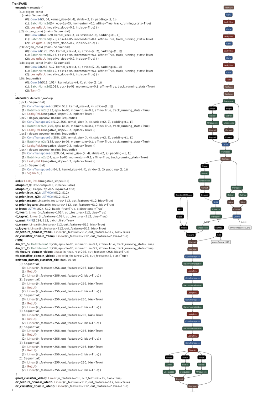
Figure 7: The neural network structure (left) and a Netron graph (right) of the proposed TranSVAE framework. Zoom-ed in for the details.

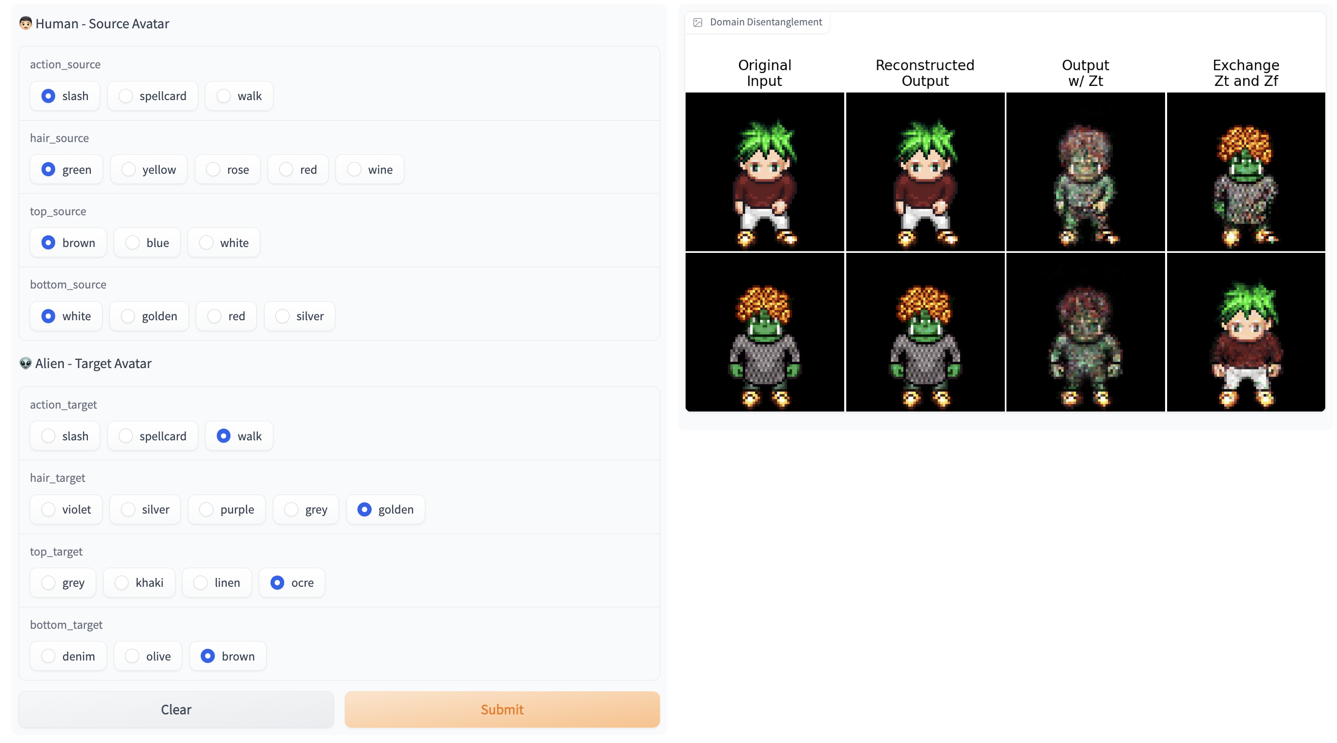
Figure 8: The input (left) and output (right) interfaces of our live demo. Users are free to customize the actions and appearances of the source and target inputs (i.e., the “Human" and “Alien" avatars) in the left-hand side and use them for disentanglement and transfer as shown in the right-hand side.

This demo is built upon Hugging Face Spaces, which provides concise and easy-to-use live demo interfaces. Our demo consists of one input interface and one output interface as shown in Fig. 8. Specifically, the appearances of the Sprites avatars are fully controlled by four attributes, i.e., body, hair color, top wear, and bottom wear. We construct two domains, $\mathbf{P}_{1}$ and $\mathbf{P}_{2}$. $\mathbf{P}_{1}$ uses the “Human” body while $\mathbf{P}_{1}$ uses the “Alien" body. The attribute pools of “Human" and “Alien" are non-overlapping across domains, resulting in completely heterogeneous $\mathbf{P}_{1}$ and $\mathbf{P}_{2}$. Each video sequence contains eight frames in total.

For conducting domain disentanglement and transfer with TranSVAE, users are free to choose the action and the appearance of the avatars on the left-hand side of the interface. Next, simply click the “Submit" button and the adaptation results will display on the right-hand side of the interface in a few seconds. The outputs include:

• The 1st column: The original input of the “Human" and “Alien" avatars, i.e., $\{\mathbf{x}_{1}^{\mathbf{P}_{1}},...,\mathbf{x}_{8}^{\mathbf{P}_{1}}\}$ and $\{\mathbf{x}_{1}^{\mathbf{P}_{2}},...,\mathbf{x}_{8}^{\mathbf{P}_{2}}\}$;

• The 2nd column: The reconstructed “Human" and “Alien" avatars $\{\widetilde{\mathbf{x}}_{1}^{\mathbf{P}_{1}},...,\widetilde{\mathbf{x}}_{8}^{\mathbf{P}_{1}}\}$ and $\{\widetilde{\mathbf{x}}_{1}^{\mathbf{P}_{2}},...,\widetilde{\mathbf{x}}_{8}^{\mathbf{P}_{2}}\}$;

• The 3rd column: The reconstructed “Human" and “Alien" avatars using only $\{\mathbf{z}_{1}^{\mathcal{D}},...,\mathbf{z}_{8}^{\mathcal{D}}\}$, $\mathcal{D}\in\{\mathbf{P}_{1},\mathbf{P}_{2}\}$, which are domain-invariant;

• The 4th column: The reconstructed “Human" and “Alien" avatars by exchanging $\mathbf{z}_{d}^{\mathcal{D}}$, which results in two sequences with the same actions but exchanged appearance, i.e., domain disentanglement and transfer.

Table 8: Ablation results without and with disentanglement term.

$\mathcal{L}_{\text{svae}}$	$\mathcal{L}_{\text{cls}}$	$\mathcal{L}_{\text{adv}}$	$\mathcal{L}_{\text{mi}}$	$\mathcal{L}_{\text{ctc}}$	$\mathbf{U}\to\mathbf{H}$	$\mathbf{H}\to\mathbf{U}$
	✓	✓			$81.67$	$90.54$
	✓		✓		$79.44$	$90.37$
	✓			✓	$81.11$	$90.37$
	✓	✓	✓	✓	$82.22$	$91.07$
✓	✓	✓			$84.44$	$93.52$
✓	✓		✓		$83.06$	$93.70$
✓	✓			✓	$83.61$	$91.42$
✓	✓	✓	✓	✓	$\mathbf{87.78}$	$\mathbf{98.95}$

Table 9: Ablation results for the frame number $T$.

Task	$5$	$6$	$7$	$8$	$9$	$10$	$12$	$14$	$16$	$20$
$\mathbf{U}\to\mathbf{H}$	$84.44$	$86.11$	$84.17$	$\mathbf{87.78}$	$84.72$	$85.28$	$83.89$	$84.44$	$82.78$	$85.00$
$\mathbf{H}\to\mathbf{U}$	$96.85$	$94.22$	$98.42$	$94.75$	$\mathbf{98.95}$	$93.70$	$93.87$	$94.40$	$94.05$	$94.40$

Table 10: Ablation results for the pseudo-label threshold $\eta$.

Task	w/o	$0.90$	$0.91$	$0.92$	$0.93$	$0.94$	$0.95$	$0.96$	$0.97$	$0.98$	$0.99$
$\mathbf{U}\to\mathbf{H}$	$87.22$ ($\mathbf{-0.56}$)	$86.94$	$87.22$	$87.50$	$\mathbf{87.78}$	$86.11$	$86.67$	$86.94$	$86.39$	$86.11$	$86.39$
$\mathbf{H}\to\mathbf{U}$	$94.40$ ($\mathbf{-4.55}$)	$98.42$	$97.37$	$98.77$	$98.60$	$98.25$	$98.25$	$\mathbf{98.95}$	$97.90$	$97.72$	$95.27$

7 Additional Experimental Results

In this section, we provide additional quantitative and qualitative results for our TranSVAE framework.

7.1 Additional Ablation Studies

Component Integration Study. We further analyze the effect of each loss term without disentanglement, i.e., not adding $\mathcal{L}_{\text{svae}}$, on the UCF-HMDB dataset, as shown in Tab. 8. Without $\mathcal{L}_{\text{svae}}$, the framework is to learn representations with corresponding constraints as many existing video-based UDA methods do. Precisely, we have the following remarks for the top-half table:

• Only with $\mathcal{L}_{\text{adv}}$, the framework is equivalent to TA³N [7], which learns the domain-invariant temporal representation. We can see the adaptation results are similar to that of [7].

• $\mathcal{L}_{\text{mi}}$ is a term specifically designed for disentanglement purposes. Thus, the effect of using $\mathcal{L}_{\text{mi}}$ alone for adaptation is random as verified in the above table, achieving worse results in the $\mathbf{U}\to\mathbf{H}$ task and better results in the $\mathbf{H}\to\mathbf{U}$ tasks compared with the source-only baseline.

• $\mathcal{L}_{\text{ctc}}$ enforces the learned static representation to be domain-specific and brings indirect benefit to adaptation, thus obtaining slightly better results than the source-only baseline.

In sum, without $\mathcal{L}_{\text{svae}}$, the adaptation performance of each loss term alone is far from optimal. Moreover, combining all the terms can slightly improve the adaptation performance over the individual ones, however, is still obviously worse than TranSVAE results. The above ablation study shows the necessity of the disentanglement in the TranSVAE framework and proves that $\mathcal{L}_{\text{svae}}$ is an indispensable loss term.

Regarding the bottom half table showing the results with $\mathcal{L}_{\text{adv}}$, we have the following remarks:

• Each individual term with $\mathcal{L}_{\text{adv}}$ achieves better adaptation results than the source-only baseline.

• Each individual term with $\mathcal{L}_{\text{adv}}$ consistently outperforms the corresponding ones without $\mathcal{L}_{\text{adv}}$.

• The final TranSVAE framework combined all the loss terms yields much better results than each individual case.

This set of ablation studies indicates that 1) each term in TranSVAE brings positive effects to adaptation, and 2) disentanglement and adaptation are interactive and complementary in our framework to obtain the best possible UDA results.

Number of Frames $T$. Tab. 9 shows the transfer performance with the variation of the number of frames $T$ on the UCF-HMDB dataset. As can be seen, the two tasks achieve the optimal performance with different $T$, specifically $T=8$ for $\mathbf{U}\to\mathbf{H}$ and $T=9$ for $\mathbf{H}\to\mathbf{U}$. Based on this observation, we apply a grid search on the validation set to obtain the optimal $T$ for each task in our experiments.

Target Pseudo-Label Threshold $\eta$. We show the sensitivity analyses of the transfer performance with respect to the target pseudo label threshold $\eta$ on the UCF-HMDB dataset in Tab. 10. The results show that different tasks yield the best transfer result with different $\eta$, specifically $\eta=0.93$ for $\mathbf{U}\to\mathbf{H}$ and $\eta=0.96$ for $\mathbf{H}\to\mathbf{U}$. Thus, we also apply the grid search on the validation set to obtain the optimal $\eta$ for each task.

7.2 Additional Qualitative Results

For those who cannot access our live demo, we have included more qualitative examples for domain disentanglement and transfer in Fig. 9. We also provide a link for GIFs demonstrating various disentanglement and reconstruction results.

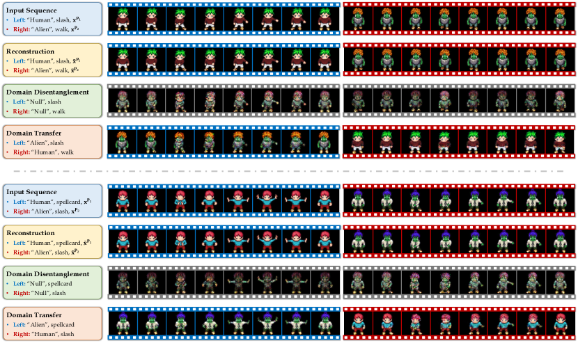
Figure 9: Additional qualitative results for illustrating the domain disentanglement and transfer properties in our TranSVAE framework.

In the GIFs link, we show two cases, the first two columns for the first one and the last two columns for the second one. Each case contains a source and a target cartoon character performing an action. For each row, we have the following remark:

• The second row shows the reconstructed results of TranSVAE, i.e. $\mathbf{z}_{d}^{\mathcal{D}}$ and $\mathbf{z}_{t}^{\mathcal{D}}$. As can be seen, TranSVAE reconstructs the image with a high quality.

• The third row shows the reconstructed results only using the static latent factors, i.e., $\mathbf{z}_{d}^{\mathcal{D}}$ and $\mathbf{0}_{t}^{\mathcal{D}}$, where we replace $\mathbf{z}_{t}^{\mathcal{D}}$ with zero vectors. As can be seen, the reconstructed results are basically static containing the appearance of the character which is the main domain difference in the Sprites dataset [22]. Specifically, we find they generally lack arms. This is reasonable as the target action is slashing or spelling cards with arms moving, and such dynamic information on the arm is captured by $\mathbf{z}_{t}^{\mathcal{D}}$.

• The fourth row shows the reconstructed results only using the dynamic latent factors, i.e., $\mathbf{0}_{d}^{\mathcal{D}}$ and $\mathbf{z}_{t}^{\mathcal{D}}$, where we replace $\mathbf{z}_{d}^{\mathcal{D}}$ with zero vectors. As can be seen, the reconstructed results are performing the right action but the appearance is mixed up. This shows that $\mathbf{z}_{t}^{\mathcal{D}}$ are indeed domain-invariant and contain the semantic information.

• The last row shows the reconstructed results of exchanging the dynamic latent factors between domains, i.e., ($\mathbf{0}_{d}^{\mathcal{S}}$, $\mathbf{z}_{t}^{\mathcal{T}}$) and ($\mathbf{0}_{d}^{\mathcal{T}}$, $\mathbf{z}_{t}^{\mathcal{S}}$). As can be seen, the reconstructed results are with the original appearance but perform the transferred action. This indicates the potential of TranSVAE for some style-transfer tasks.

8 Broader Impact

This paper provides a novel transfer method to use cross-domain video data, which effectively helps reduce the annotation efforts in related video applications. Although the main empirical evaluation is on the video action recognition task, the model structure proposed in this paper is also applicable to other video-related tasks, such as action segmentation, video semantic segmentation, etc. More generally, the idea of disentangling domain information sheds light on other data modality style transfer tasks, e.g., voice conversion. The negative impacts of this work are difficult to predict. However, as a deep model, our method shares some common pitfalls of the standard deep learning models, e.g., demand for powerful computing resources, and vulnerability to adversarial attacks.

9 Public Resources Used

We acknowledge the use of the following public resources, during the course of this work:

• UCF₁₀₁Unknown

• HMDB₅₁CC BY 4.0

• JesterUnknown

• Epic-KitchensCC BY-NC 4.0

• SpritesCC-BY-SA-3.0

• I3DApache License 2.0

• TRNBSD 2-Clause License

• CoMixApache License 2.0

• TA³NMIT License

• CO²AUnknown

• PyTorchPyTorch Custom License

• NetronMIT License

• flops-counter.pytorchMIT License

References

- [1] Junwen Bai, Weiran Wang, and Carla P Gomes. Contrastively disentangled sequential variational autoencoder. In Advances in Neural Information Processing Systems, volume 34, pages 10105–10118, 2021.
- [2] Lejla Batina, Benedikt Gierlichs, Emmanuel Prouff, Matthieu Rivain, François-Xavier Standaert, and Nicolas Veyrat-Charvillon. Mutual information analysis: a comprehensive study. Journal of Cryptology, 24(2):269–291, 2011.
- [3] Qi Cai, Yingwei Pan, Chong-Wah Ngo, Xinmei Tian, Lingyu Duan, and Ting Yao. Exploring object relation in mean teacher for cross-domain detection. In IEEE/CVF Conference on Computer Vision and Pattern Recognition, pages 11457–11466, 2019.
- [4] Ruichu Cai, Zijian Li, Pengfei Wei, Jie Qiao, Kun Zhang, and Zhifeng Hao. Learning disentangled semantic representation for domain adaptation. In International Joint Conferences on Artificial Intelligence, volume 2019, page 2060, 2019.
- [5] Ruichu Cai, Fengzhu Wu, Zijian Li, Pengfei Wei, Lingling Yi, and Kun Zhang. Graph domain adaptation: A generative view. arXiv preprint arXiv:2106.07482, 2021.
- [6] Joao Carreira and Andrew Zisserman. Quo vadis, action recognition? a new model and the kinetics dataset. In IEEE/CVF Conference on Computer Vision and Pattern Recognition, pages 6299–6308, 2017.
- [7] Min-Hung Chen, Zsolt Kira, Ghassan AlRegib, Jaekwon Yoo, Ruxin Chen, and Jian Zheng. Temporal attentive alignment for large-scale video domain adaptation. In IEEE/CVF International Conference on Computer Vision, pages 6321–6330, 2019.
- [8] Peipeng Chen, Yuan Gao, and Andy J Ma. Multi-level attentive adversarial learning with temporal dilation for unsupervised video domain adaptation. In IEEE/CVF Winter Conference on Applications of Computer Vision, pages 1259–1268, 2022.
- [9] Ricky TQ Chen, Xuechen Li, Roger B Grosse, and David K Duvenaud. Isolating sources of disentanglement in variational autoencoders. In Advances in Neural Information Processing Systems, volume 31, pages 1–11, 2018.
- [10] Jinwoo Choi, Gaurav Sharma, Samuel Schulter, and Jia-Bin Huang. Shuffle and attend: Video domain adaptation. In European Conference on Computer Vision, pages 678–695. Springer, 2020.
- [11] Dima Damen, Hazel Doughty, Giovanni Maria Farinella, Sanja Fidler, Antonino Furnari, Evangelos Kazakos, Davide Moltisanti, Jonathan Munro, Toby Perrett, Will Price, et al. Scaling egocentric vision: The epic-kitchens dataset. In European Conference on Computer Vision, pages 720–736. Springer, 2018.
- [12] Avijit Dasgupta, CV Jawahar, and Karteek Alahari. Overcoming label noise for source-free unsupervised video domain adaptation. In Proceedings of the Thirteenth Indian Conference on Computer Vision, Graphics and Image Processing, pages 1–9, 2022.
- [13] Wanxia Deng, Lingjun Zhao, Qing Liao, Deke Guo, Gangyao Kuang, Dewen Hu, Matti Pietikäinen, and Li Liu. Informative feature disentanglement for unsupervised domain adaptation. IEEE Transactions on Multimedia, 24:2407–2421, 2021.
- [14] Yaroslav Ganin, Evgeniya Ustinova, Hana Ajakan, Pascal Germain, Hugo Larochelle, François Laviolette, Mario Marchand, and Victor Lempitsky. Domain-adversarial training of neural networks. Journal of Machine Learning Research, 17(1):2096–2030, 2016.
- [15] Dayan Guan, Jiaxing Huang, Aoran Xiao, Shijian Lu, and Yanpeng Cao. Uncertainty-aware unsupervised domain adaptation in object detection. IEEE Transactions on Multimedia, 24:2502–2514, 2021.
- [16] Maximilian Ilse, Jakub M Tomczak, Christos Louizos, and Max Welling. Diva: Domain invariant variational autoencoders. In Medical Imaging with Deep Learning, pages 322–348. PMLR, 2020.
- [17] Will Kay, Joao Carreira, Karen Simonyan, Brian Zhang, Chloe Hillier, Sudheendra Vijayanarasimhan, Fabio Viola, Tim Green, Trevor Back, Paul Natsev, et al. The kinetics human action video dataset. arXiv preprint arXiv:1705.06950, 2017.
- [18] Donghyun Kim, Yi-Hsuan Tsai, Bingbing Zhuang, Xiang Yu, Stan Sclaroff, Kate Saenko, and Manmohan Chandraker. Learning cross-modal contrastive features for video domain adaptation. In IEEE/CVF International Conference on Computer Vision, pages 13618–13627, 2021.
- [19] Lingdong Kong, Niamul Quader, and Venice Erin Liong. Conda: Unsupervised domain adaptation for lidar segmentation via regularized domain concatenation. In IEEE International Conference on Robotics and Automation, pages 9338–9345, 2023.
- [20] Hildegard Kuehne, Hueihan Jhuang, Estíbaliz Garrote, Tomaso Poggio, and Thomas Serre. Hmdb: a large video database for human motion recognition. In IEEE/CVF International Conference on Computer Vision, pages 2556–2563. IEEE, 2011.
- [21] Yanghao Li, Naiyan Wang, Jianping Shi, Xiaodi Hou, and Jiaying Liu. Adaptive batch normalization for practical domain adaptation. Pattern Recognition, 80:109–117, 2018.
- [22] Yingzhen Li and Stephan Mandt. Disentangled sequential autoencoder. In International Conference on Machine Learning, pages 5670–5679. PMLR, 2018.
- [23] Wei Lin, Anna Kukleva, Kunyang Sun, Horst Possegger, Hilde Kuehne, and Horst Bischof. Cycda: Unsupervised cycle domain adaptation to learn from image to video. In European Conference on Computer Vision, pages 698–715. Springer, 2022.
- [24] Youquan Liu, Lingdong Kong, Jun Cen, Runnan Chen, Wenwei Zhang, Liang Pan, Kai Chen, and Ziwei Liu. Segment any point cloud sequences by distilling vision foundation models. arXiv preprint arXiv:2306.09347, 2023.
- [25] Mingsheng Long, Han Zhu, Jianmin Wang, and Michael I Jordan. Deep transfer learning with joint adaptation networks. In International Conference on Machine Learning, pages 2208–2217. PMLR, 2017.
- [26] Yadan Luo, Zi Huang, Zijian Wang, Zheng Zhang, and Mahsa Baktashmotlagh. Adversarial bipartite graph learning for video domain adaptation. In ACM International Conference on Multimedia, pages 19–27, 2020.
- [27] Joanna Materzynska, Guillaume Berger, Ingo Bax, and Roland Memisevic. The jester dataset: A large-scale video dataset of human gestures. In IEEE/CVF International Conference on Computer Vision Workshops, pages 1–12, 2019.
- [28] Jonathan Munro and Dima Damen. Multi-modal domain adaptation for fine-grained action recognition. In IEEE/CVF Conference on Computer Vision and Pattern Recognition, pages 122–132, 2020.
- [29] Boxiao Pan, Zhangjie Cao, Ehsan Adeli, and Juan Carlos Niebles. Adversarial cross-domain action recognition with co-attention. In AAAI Conference on Artificial Intelligence, pages 11815–11822, 2020.
- [30] Adam Paszke, Sam Gross, Francisco Massa, Adam Lerer, James Bradbury, Gregory Chanan, Trevor Killeen, Zeming Lin, Natalia Gimelshein, Luca Antiga, Alban Desmaison, Andreas Kopf, Edward Yang, Zachary DeVito, Martin Raison, Alykhan Tejani, Sasank Chilamkurthy, Benoit Steiner, Lu Fang, Junjie Bai, and Soumith Chintala. Pytorch: An imperative style, high-performance deep learning library. In Advances in Neural Information Processing Systems, 2019.
- [31] Aadarsh Sahoo, Rutav Shah, Rameswar Panda, Kate Saenko, and Abir Das. Contrast and mix: Temporal contrastive video domain adaptation with background mixing. In Advances in Neural Information Processing Systems, volume 34, pages 23386–23400, 2021.
- [32] Kuniaki Saito, Kohei Watanabe, Yoshitaka Ushiku, and Tatsuya Harada. Maximum classifier discrepancy for unsupervised domain adaptation. In IEEE/CVF Conference on Computer Vision and Pattern Recognition, pages 3723–3732, 2018.
- [33] Antoine Saporta, Arthur Douillard, Tuan-Hung Vu, Patrick Pérez, and Matthieu Cord. Multi-head distillation for continual unsupervised domain adaptation in semantic segmentation. In IEEE/CVF Conference on Computer Vision and Pattern Recognition, pages 3751–3760, 2022.
- [34] Xiaolin Song, Sicheng Zhao, Jingyu Yang, Huanjing Yue, Pengfei Xu, Runbo Hu, and Hua Chai. Spatio-temporal contrastive domain adaptation for action recognition. In IEEE/CVF Conference on Computer Vision and Pattern Recognition, pages 9787–9795, 2021.
- [35] Khurram Soomro, Amir Roshan Zamir, and Mubarak Shah. Ucf101: A dataset of 101 human actions classes from videos in the wild. arXiv preprint arXiv:1212.0402, 2012.
- [36] Zhan Tong, Yibing Song, Jue Wang, and Limin Wang. Videomae: Masked autoencoders are data-efficient learners for self-supervised video pre-training. Advances in Neural Information Processing Systems, 35:10078–10093, 2022.
- [37] Victor G Turrisi, Giacomo Zara, Paolo Rota, Thiago Oliveira-Santos, Nicu Sebe, Vittorio Murino, and Elisa Ricci. Dual-head contrastive domain adaptation for video action recognition. In IEEE/CVF Winter Conference on Applications of Computer Vision, pages 2234–2243, 2022.
- [38] Eric Tzeng, Judy Hoffman, Kate Saenko, and Trevor Darrell. Adversarial discriminative domain adaptation. In IEEE/CVF Conference on Computer Vision and Pattern Recognition, pages 7167–7176, 2017.
- [39] Laurens Van der Maaten and Geoffrey Hinton. Visualizing data using t-sne. Journal of Machine Learning Research, 9(11), 2008.
- [40] Limin Wang, Bingkun Huang, Zhiyu Zhao, Zhan Tong, Yinan He, Yi Wang, Yali Wang, and Yu Qiao. Videomae v2: Scaling video masked autoencoders with dual masking. In IEEE/CVF Conference on Computer Vision and Pattern Recognition, pages 14549–14560, 2023.
- [41] Garrett Wilson and Diane J Cook. A survey of unsupervised deep domain adaptation. ACM Transactions on Intelligent Systems and Technology, 11(5):1–46, 2020.
- [42] Ni Xiao and Lei Zhang. Dynamic weighted learning for unsupervised domain adaptation. In IEEE/CVF Conference on Computer Vision and Pattern Recognition, pages 15242–15251, 2021.
- [43] Lijin Yang, Yifei Huang, Yusuke Sugano, and Yoichi Sato. Interact before align: Leveraging cross-modal knowledge for domain adaptive action recognition. In IEEE/CVF Conference on Computer Vision and Pattern Recognition, pages 14722–14732, 2022.
- [44] Yuehao Yin, Bin Zhu, Jingjing Chen, Lechao Cheng, and Yu-Gang Jiang. Mix-dann and dynamic-modal-distillation for video domain adaptation. In ACM International Conference on Multimedia, pages 3224–3233, 2022.
- [45] Fuxun Yu, Di Wang, Yinpeng Chen, Nikolaos Karianakis, Tong Shen, Pei Yu, Dimitrios Lymberopoulos, Sidi Lu, Weisong Shi, and Xiang Chen. Sc-uda: Style and content gaps aware unsupervised domain adaptation for object detection. In IEEE/CVF Winter Conference on Applications of Computer Vision, pages 382–391, 2022.
- [46] Yang Yu, Zhiqiang Gong, Ping Zhong, and Jiaxin Shan. Unsupervised representation learning with deep convolutional neural network for remote sensing images. In International Conference on Image and Graphics, pages 97–108. Springer, 2017.
- [47] Jingyi Zhang, Jiaxing Huang, Zichen Tian, and Shijian Lu. Spectral unsupervised domain adaptation for visual recognition. In IEEE/CVF Conference on Computer Vision and Pattern Recognition, pages 9829–9840, 2022.
- [48] Yunhua Zhang, Hazel Doughty, Ling Shao, and Cees GM Snoek. Audio-adaptive activity recognition across video domains. In IEEE/CVF Conference on Computer Vision and Pattern Recognition, pages 13791–13800, 2022.
- [49] Bolei Zhou, Alex Andonian, Aude Oliva, and Antonio Torralba. Temporal relational reasoning in videos. In European Conference on Computer Vision, pages 803–818. Springer, 2018.
- [50] Yizhe Zhu, Martin Renqiang Min, Asim Kadav, and Hans Peter Graf. S3vae: Self-supervised sequential vae for representation disentanglement and data generation. In IEEE/CVF Conference on Computer Vision and Pattern Recognition, pages 6538–6547, 2020.
- [51] Yang Zou, Zhiding Yu, BVK Kumar, and Jinsong Wang. Unsupervised domain adaptation for semantic segmentation via class-balanced self-training. In European Conference on Computer Vision, pages 289–305. Springer, 2018.