A statistical mechanics framework for polymer chain scission, based on the concepts of distorted bond potential and asymptotic matching

Abstract

To design increasingly tough, resilient, and fatigue-resistant elastomers and hydrogels, the relationship between controllable network parameters at the molecular level (bond type, non-uniform chain length, entanglement density, etc.) to macroscopic quantities that govern damage and failure must be established. Many of the most successful constitutive models for elastomers have been rooted in statistical mechanical treatments of polymer chains. Typically, such constitutive models have used variants of the freely jointed chain model with rigid links. However, since the free energy state of a polymer chain is dominated by enthalpic bond distortion effects as the chain approaches its rupture point, bond extensibility ought to be accounted for if the model is intended to capture chain rupture. To that end, a new bond potential is supplemented to the freely jointed chain model (as derived in the $u$FJC framework of buche2021chain and buche2022freely), which we have extended to yield a tractable, closed-form model that is amenable to constitutive model development. Inspired by the asymptotically matched $u$FJC model response in both the low/intermediate chain force and high chain force regimes, a simple, quasi-polynomial bond potential energy function is derived. This bond potential exhibits harmonic behavior near the equilibrium state and anharmonic behavior for large bond stretches tending to a characteristic energy plateau (akin to the Lennard-Jones and Morse bond potentials). Using this bond potential, approximate yet highly-accurate analytical functions for bond stretch and chain force dependent upon chain stretch are established. Then, using this polymer chain model, a stochastic thermal fluctuation-driven chain rupture framework is developed. This framework is based upon a force-modified tilted bond potential that accounts for distortional bond potential energy, allowing for the derivation and subsequent calculation of the dissipated chain scission energy. The cases of rate-dependent and rate-independent scission are accounted for throughout the rupture framework. The impact of Kuhn segment number on chain rupture behavior is also investigated. The model is fit to single-chain mechanical response data collected from atomic force microscopy tensile tests for validation and to glean deeper insight into the molecular physics taking place. Due to their analytical nature, this polymer chain model and the associated rupture framework can be straightforwardly implemented in finite element models accounting for fracture and fatigue in polydisperse elastomer networks.

1 Introduction

Elastomers are materials composed of flexible entropic polymer chains oriented randomly, cross-linked together, and arranged in a network structure. Due to their resilience and ability to undergo large and recoverable deformations, elastomers have been used as components in traditional engineering applications, such as tires, belts, and sealers (gent2012engineering). More recently, elastomers have emerged as ideal candidate materials for next-generation soft robotics components and biomedical devices (zhalmuratova2020reinforced). As elastomers with covalent cross-links become increasingly deformed, polymer chains begin to elongate, and bonds composing the backbone of these chains become stretched. Eventually, these bonds or the bonds of the cross-links rupture. These discrete rupture events collectively build up in the elastomer network and ultimately lead to macroscale failure of the bulk specimen. Additionally, these chain rupture events serve to dissipate energy imparted to the network, and enhance network toughness. This work will focus on rupture events impacting the chain backbone directly (and not the cross-links).

Understanding the fundamentals of energy dissipation, network toughness, and fracture mechanics in elastomers and gels has been an active area of research in recent years (long2021fracture; zhao2021soft; bai2019fatigue; creton201750th; creton2016fracture; long2016fracture; zhao2014multi). One overarching takeaway from this thrust of research is that the fracture energy of a soft elastomer network, $\Gamma$, namely, the energy required to form new unit crack surface area in the bulk material, can be considered as the sum result of two contributions (long2021fracture; zhao2021soft; long2016fracture; zhao2014multi; tanaka2007local)

$$\Gamma=\Gamma_{0}+\Gamma_{diss},$$ (1)

where $\Gamma_{0}$ is the intrinsic fracture energy and $\Gamma_{diss}$ is the mechanical dissipation that takes place in a process zone surrounding the crack tip. Due to the random topology of the chain network, and the naturally occurring polydispersity of chain lengths that arises due to polymerization statistics, which can be thought of as network imperfections, chain rupture can occur in a delocalized manner in the elastomer (itskov2016rubber; yang2019polyacrylamide). $\Gamma_{diss}$ is generated from any dissipative phenomena that occurs during crack propagation, such as delocalized chain scission, molecular friction due to entanglements and chain pullout, viscoelasticity, poroelasticity, strain-induced crystallization, and polymer-filler interactions. The size of this process zone that is responsible for $\Gamma_{diss}$ can range in length as different dissipation mechanisms become prominent. Various elastomer network characteristics govern how large $\Gamma_{diss}$ is compared to $\Gamma_{0}$. In ideal elastomer networks, $\Gamma_{diss}\approxeq 0$ and $\Gamma/\Gamma_{0}\approxeq 1$, even with a small density of topological defects incorporated in the network (lin2021fracture). $\Gamma_{diss}\approxeq 0$ and $\Gamma/\Gamma_{0}\approxeq 1$ also holds true for nearly unentangled networks, even with structural heterogeneities and topological defects present (zheng2022fracture). On the contrary, in entangled elastomer networks, $\Gamma_{diss}>0$ and $\Gamma/\Gamma_{0}>1$, where the fracture toughness enhancement is postulated to originate from chain pullout and delocalized chain damage in a near-crack process zone (zheng2022fracture; kim2021fracture). In elastomer networks containing notable amounts of network imperfections from structural heterogeneities, topological defects, and even pre-existing cracks in the bulk material, $\Gamma_{diss}>0$ and $\Gamma/\Gamma_{0}>1$ is also found to be the case (yang2019polyacrylamide; liu2019polyacrylamide). Here, fracture toughness enhancement and elastic dissipation are believed to stem from delocalized chain scission (yang2019polyacrylamide; liu2019polyacrylamide).

To reveal and better understand the complex molecular behavior of polymer chains in fractured, and more generally, damaged elastomers, mechanophores have been incorporated into elastomer networks to probe force-activated events originating at the chain level (chen2021mechanochemical; stratigaki2020methods; simon2017mechanochemistry). Mechanophore motifs that alter their optical properties with respect to applied load – mechanochromophores and/or mechanofluorophores (hereafter referred to as luminescent mechanophores) – have emerged as the preferred tool to visualize such force-sensitive chain level behavior (chen2021mechanochemical; gostl2017optical). Embedded luminescent mechanophores in elastomer networks have confirmed that chains located far from the crack surface (compared to the chain length) become ruptured during crack advance (ducrot2014toughening; slootman2020quantifying; matsuda2021revisiting; boots2022quantifying; matsuda2020crack), supporting the postulated mechanism of dissipation and toughness enhancement. Unsurprisingly, viscoelastic effects and microscopic dynamics have been found to influence and interplay with the extent of delocalized chain scission measured via luminescent mechanophores (slootman2020quantifying; slootman2022molecular). Embedded luminescent mechanophores have also been used to visualize delocalized chain scission in elastomer networks undergoing cavitation (morelle20213d; kim2020extreme) and fatigue (sanoja2021mechanical).

To develop a model that accounts for the collective impact delocalized chain rupture events play on the bulk material response, and more specifically on the fracture energy, several key building blocks are needed. Incorporating a chain length distribution to reflect the structural heterogeneity of non-uniform chain length in an elastomer network is a vital starting point that has already been proven to impact elastomer mechanics and fracture (falender1979effect; mark2003elastomers; dargazany2009network; wang2015mechanics; itskov2016rubber; diani2019fully; lavoie2019modeling; li2020variational; lu2020pseudo; mulderrig2021affine; guo2021micromechanics; xiao2021modeling). Incorporation of chain length polydispersity into the network requires defining the chain-level load sharing behavior. The equal strain assumption is commonly employed, where all chains, independent of initial length, are assumed to be deformed to the same stretch (itskov2016rubber; tehrani2017effect; diani2019fully; mulderrig2021affine). The equal force assumption may also be implemented, where all chains are assumed to bear the same force (via a virtual series arrangement of chains with respect to the loading mechanism) (verron2017equal; li2020variational; mulderrig2021affine). Connecting the chain-level deformation with the continuum-level deformation has been possible through homogenization assumptions, including the affine three-chain model (wang1952statistical), non-affine four-chain model (flory1943statistical), non-affine Arruda-Boyce eight-chain model (arruda1993three), affine full-network microsphere model (treloar1979non; wu1992improved; wu1993improved), and non-affine full-network microsphere models (miehe2004micro; tkachuk2012maximal; diani2019fully; ghaderi2020physics; mulderrig2021affine; rastak2018non; arunachala2021energy; guo2021micromechanics). The interplay between chain-level load sharing with the macro-to-micro deformation relationship has been shown to exert a significant role in local strain-stiffening and delocalized chain rupture (tauber2021sharing; tauber2022stretchy; basu2011nonaffine; black2011molecular; chen2021mechanochemistry; chen2020force; mulderrig2021affine).

A molecular description of chain rupture leading to macroscopic damage and failure is the final building block to address. Such a description of chain rupture requires acccounting for bond extensibility in single chain elasticity and relating the state of the chain to its state of rupture. Bond extensibility is an inherent necessity in a chain rupture model because the rupture of chains along the fracture plane in elastomer networks is enthalpically dominated (not entropically dominated), as recognized by lake1967strength. smith1996overstretching proposed a phenomenological modification of the Langevin-statistics based freely-jointed chain (FJC) model of kuhn1942beziehungen to account for the influence of bond extensibility. Inspired by this work, mao2017rupture took the Langevin-statistics based FJC Helmholtz free energy function, permitted bonds to vary in length, added an internal potential energy of bond stretching to the free energy, and heuristically forced the bond stretch to be the minimizer of this modified Helmholtz free energy. Bond extensibility can also be incorporated in a statistical mechanics-consistent extensible FJC model, as achieved recently by buche2021chain and buche2022freely utilizing asymptotic matching. Notably, the $u$FJC model of buche2021chain and buche2022freely accounts for arbitrary bond extensibility, i.e., the influence of extensible bonds are theoretically incorporated in the $u$FJC model prior to any particularization of a governing bond potential energy function. Once the entropic and enthalpic contributions are defined, the statistics of rupture for a given population of chains can be studied. One way to resolve the statistics of chain rupture is to consider fully intact chains as automatically ruptured when their free energy or internal energy exceeds some rupture energy (or when their chain force exceeds its maximum value) (mao2017rupture; arunachala2021energy; lamont2021rate; xiao2021modeling; zhao2021multiscale; dal2009micro; buche2021chain). Another approach is to define a thermodynamically-consistent damage law (often dependent on the bond stretch) that accounts for network softening. This can also be employed in a phase field fracture setting (mao2018theory; talamini2018progressive; li2020variational; mulderrig2021affine). Alternatively, consistent with statistical thermodynamics, chain scission can be treated as a stochastic process driven by thermal oscillations (arora2020fracture; arora2021coarse; lu2020pseudo; yang2020multiscale; lei2022multiscale; guo2021micromechanics). Strikingly, the extensible chain model used within the last two (more descriptive) treatments of chain rupture is, to date, solely the mao2017rupture phenomenologically modified FJC model. In other words, an extensible FJC model derived thoroughly upon statistical mechanics principles has yet to be embedded within either a damage law-based treatment or a stochastic treatment of chain rupture.

In this manuscript, we develop a framework to study polymer chain scission, where its novelty lies upon two key pillars: (i) an arbitrarily-extensible FJC model derived entirely through statistical mechanics that also respects the principles of statistical thermodynamics and asymptotic matching, and (ii) a probabilistic understanding of chain scission, starting from a consideration of thermal oscillations and rupture at the segment level, consistent with the principles of mechanochemistry. To address the first pillar, we extend the $u$FJC model from buche2021chain and buche2022freely to yield an analytical form for the chain force and the Helmholtz free energy function (also seeking to connect to the prevalent phenomenological functional form proposed in mao2017rupture). Using the principles of asymptotic matching (as employed in the derivation of the $u$FJC model), a simple, anharmonic, quasi-polynomial potential energy function for a segment (or a bond) in a chain is derived. From this potential energy function, a highly-accurate approximate analytical form for segment stretch as a function of chain stretch is obtained. To address the second pillar, rate-dependent and rate-independent segment scission is treated as a stochastic, energy-activated process as captured via the force-modified tilted potential energy. Principles of scission physics as described in wang2019quantitative are evoked to derive the governing equations for rate-dependent and rate-independent dissipated chain scission energy. A functional form for the reference end-to-end chain distance is then derived that fully accounts for segment extensibility and chain length polydispersity. This proposed polymer chain rupture framework exhibits many beneficial properties; it is clearly based upon statistical mechanics principles accounting for bond extensibility, satisfies principles of statistical thermodynamics and asymptotic matching, accounts for scission originating from the molecular level of the bond, and provides a clear multiscale connection between the physics at the bond-level, segment-level, and chain-level. Ideally, the proposed chain rupture framework can be incorporated into future polymer damage and fracture models to gain insight into the complex nature of polymer network fracture toughness.

This manuscript is organized as follows: In Section 2, the fundamentals of the $u$FJC model from buche2021chain and buche2022freely are reviewed. The $u$FJC model is then extended in Section 3 to ensure that an upscaled continuum model is defined in terms of tractable closed-form solutions. The analytical form for the chain force is determined in Section 3.1. The asymptotically-matched segment potential energy function is derived in Section 3.2.1 and LABEL:app:modulation-parameter-definition, leading to the highly-accurate approximate analytical form for segment stretch as a function of chain stretch as derived in Section 3.2.2 and LABEL:app:analytical-form-segment-stretch-function. With the chain model complete, the chain rupture framework is developed in LABEL:sec:single-chain-scission. Starting at the segment level in LABEL:subsec:segment-scission, the probability of rate-dependent and rate-independent segment scission is adopted from the principles of mechanochemistry, which consider segment scission as a stochastic process driven by thermal fluctuations and dependent upon the applied load to the segment. Governing equations for rate-dependent and rate-independent dissipated segment scission energy are then formulated. The segment scission framework is pushed up to the chain level via probabilistic considerations in LABEL:subsec:chain-scission. In LABEL:subsec:chain-scission-informed-equil-prob-dist, the functional form for the reference end-to-end chain distance dependent upon segment extensibility and segment number is derived through statistical mechanics considerations from buche2021chain. Verification and validation take place in LABEL:sec:single-chain-model-behavior-results. LABEL:subsec:single-chain-mechanical-response presents the single chain model mechanical response. Implications of the chain scission framework are discussed in LABEL:subsec:chain-scission-framework-implications, and chain rupture behavior for short, intermediately-long, and long chains is investigated in LABEL:subsec:single-chain-scission-results. In LABEL:subsec:experimental-fits, single chain mechanical response data generated from atomic force microscopy (AFM) tensile tests are used to validate the chain model. The chain rupture framework is called upon to uncover the level of dissipated energy and chain scission probability for the chains involved in the AFM tensile tests. Concluding remarks, improvements for future work, and implications for future research in elastomer fracture and fatigue modeling are highlighted in LABEL:sec:conclusion.

2 $u$FJC model review

Before defining a framework for the statistics of chain scission, the constitutive behavior of a single polymer chain must be specified. Since polymer chain rupture is an enthalpically dominated process (lake1967strength), the chain model must account for bond extensibility. The $u$FJC model has recently emerged as the first polymer chain model to intrinsically account for arbitrary segment extensibility within a statistical mechanics framework. In the following, a brief review of the $u$FJC model framework is provided as a means of establishing the proper context for the remainder of this work. This review (which will occupy the entirety of Section 2) is a summary of the most relevant results from buche2021chain and buche2022freely (unless otherwise noted).

2.1 Statistical thermodynamics foundation

The $u$FJC is a freely jointed chain of $\nu$ massless, flexible, and stretchable links, or Kuhn segments, connecting $\nu+1$ point masses with mass $m$ and momentum $p$. The segment stretch $\lambda_{\nu}$ is taken as the ratio of the segment length $l_{\nu}$ with the equilibrium segment length $l_{\nu}^{eq}$, $\lambda_{\nu}=l_{\nu}/l_{\nu}^{eq}$. The energy state of each segment is described by the (arbitrary and non-particularized) segment potential $U_{\nu}$, which inherently exhibits some characteristic segment potential energy scale $E_{\nu}^{char}$ and segment stiffness $k_{\nu}$ defined as

$$k_{\nu}\equiv U_{\nu}^{\prime\prime}(l_{\nu}^{eq})=\partialderivative[2]{U_{\nu}(l_{\nu})}{l_{\nu}}\bigg{|}_{l_{\nu}=l_{\nu}^{eq}},$$ (2)

where primes imply derivatives. Assuming fixed absolute temperature $T$, a fixed inverse energy scale can be defined as $\beta=1/[k_{B}T]$ where $k_{B}$ is the Boltzmann constant. Then, the nondimensional characteristic segment potential energy scale and nondimensional segment stiffness are respectively defined as $\zeta_{\nu}^{char}\equiv\beta E_{\nu}^{char}$ and $\kappa_{\nu}\equiv\beta[l_{\nu}^{eq}]^{2}k_{\nu}$. The single chain Hamiltonian of the $u$FJC model is

$$H(\mathscr{P})=\sum_{i=1}^{\nu+1}\frac{p_{i}^{2}}{2m}+\sum_{i=1}^{\nu}U_{\nu}(l_{\nu i})=\sum_{i=1}^{\nu+1}\frac{p_{i}^{2}}{2m}+\sum_{i=1}^{\nu}U_{\nu i},$$ (3)

where $\mathscr{P}$ is the phase space state of the chain. The single-segment isotensional configuration partition function is (buche2020statistical)

$$\mathcal{Z}_{\nu}(\xi_{c})=\int_{0}^{\pi}\int_{0}^{2\pi}\int_{0}^{\infty}e^{\beta f_{c}l_{\nu}\cos{\theta}}e^{-\beta U_{\nu}(l_{\nu})}dl_{\nu}d\phi d\theta,$$ (4)

where $f_{c}$ is the chain force, $\xi_{c}=\beta f_{c}l_{\nu}^{eq}$ is its nondimensional counterpart, and $\theta$ is the angle between the segment and the chain force. The chain isotensional configuration partition function is $\mathcal{Z}(\xi_{c})=[\mathcal{Z}_{\nu}(\xi_{c})]^{\nu}$ (fiasconaro2019analytical). The mechanical response of the chain vis-à-vis the equilibrium chain stretch $\lambda_{c}^{eq}$ is defined and provided (buche2020statistical) as

$$\lambda_{c}^{eq}(\xi_{c})=\lambda_{c}(\xi_{c})*\mathcal{A}_{\nu}=\frac{1}{\nu}\partialderivative{\ln(\mathcal{Z}(\xi_{c}))}{\xi_{c}}=\partialderivative{\ln(\mathcal{Z}_{\nu}(\xi_{c}))}{\xi_{c}}=\frac{r_{\nu}(\xi_{c})}{\nu l_{\nu}^{eq}}.$$ (5)

Here, $r_{\nu}$ is the end-to-end chain distance, $\lambda_{c}=r_{\nu}/r_{\nu}^{ref}$ is the chain stretch, $r_{\nu}^{ref}$ is the reference end-to-end chain distance, and $\mathcal{A}_{\nu}=r_{\nu}^{ref}/[\nu l_{\nu}^{eq}]$ is the reference equilibrium chain stretch.

Obtaining an analytical form for $\lambda_{c}^{eq}$ valid over all $\xi_{c}$ regimes and intrinsically accounting for arbitrary segment extensibility (as governed by $U_{\nu}(l_{\nu})$) is seemingly an impossible task. However, an analytical form is needed here for computational simplicity. To resolve this conundrum, asymptotic approximations for $\lambda_{c}^{eq}$ are derived in the low-to-intermediate chain force regime and in the high chain force regime, both of which are valid only under steep segment potentials $U_{\nu}(l_{\nu})$. The segment potential is considered to be steep if it is deep and narrow, which is true when $\zeta_{\nu}^{char}$ and $\kappa_{\nu}$ are large (i.e., $\zeta_{\nu}^{char},\kappa_{\nu}\gg 1$). The asymptotic approximations for $\lambda_{c}^{eq}$ are then combined via Prandtl’s method of asymptotic matching into a composite function valid for all $\xi_{c}$. In the limit of sufficiently steep segment potentials, this asymptotically-matched equilibrium chain stretch function is further reduced into a particularly useful analytical form.

2.2 Low-to-intermediate chain force regime

For chain forces that are both low (i.e., $\xi_{c}<1$) and intermediate (i.e., $1<\xi_{c}\ll\zeta_{\nu}^{char},\kappa_{\nu}$) and considering steep segment potentials ($\zeta_{\nu}^{char},\kappa_{\nu}\gg 1$), Laplace’s method and various asymptotic considerations are employed to evaluate Eq. 4 to the following asymptotic relation:

$$\mathcal{Z}_{\nu}(\xi_{c})\approx 4\pi[l_{\nu}^{eq}]^{3}\sqrt{\frac{2\pi}{\kappa_{\nu}}}\frac{\sinh(\xi_{c})}{\xi_{c}}e^{\frac{\xi_{c}^{2}}{2\kappa_{\nu}}}\left[1+\frac{1}{\tilde{c}_{\nu}}\frac{\xi_{c}}{\kappa_{\nu}}\coth(\xi_{c})\right],$$ (6)

where $1/\tilde{c}_{\nu}\equiv 1-u_{\nu}^{\prime\prime\prime}(1)/(2u_{\nu}^{\prime\prime}(1))$, $u_{\nu}(x)\equiv\beta U_{\nu}(xl_{\nu}^{eq})$ is the nondimensional segment potential, and $x$ is a dummy variable (for now. Later on, $x$ will be identified as the segment stretch $\lambda_{\nu}$). The corresponding asymptotic relation for the equilibrium chain stretch is

$$\lambda_{c}^{eq}(\xi_{c})\approx\mathcal{L}(\xi_{c})+\frac{\xi_{c}}{\kappa_{\nu}}\left[1+\frac{1-\mathcal{L}(\xi_{c})\coth(\xi_{c})}{\tilde{c}_{\nu}+\frac{\xi_{c}}{\kappa_{\nu}}\coth(\xi_{c})}\right],$$ (7)

where $\mathcal{L}(y)=\coth{y}-\frac{1}{y}$ is the Langevin function.

2.3 High chain force regime

For high chain forces (i.e., $\xi_{c}=\text{ord}(\zeta_{\nu}^{char})$) and with steep segment potentials ($\zeta_{\nu}^{char},\kappa_{\nu}\gg 1$), asymptotic considerations are employed to simplify Eq. 4 to the following asymptotic relation:

$$\mathcal{Z}_{\nu}(\xi_{c})\approx\frac{2\pi[l_{\nu}^{eq}]^{3}}{\xi_{c}}\int_{0}^{\infty}e^{-u_{\nu}^{tot}(x)}xdx,$$ (8)

where $u_{\nu}^{tot}$ is the nondimensional total segment potential, defined as

$$u_{\nu}^{tot}(x)\equiv u_{\nu}(x)-\xi_{c}x.$$ (9)

The corresponding asymptotic relation for $\lambda_{c}^{eq}$ is

$$\lambda_{c}^{eq}(\xi_{c})\approx\frac{\int_{0}^{\infty}e^{-u_{\nu}^{tot}(x)}x^{2}dx}{\int_{0}^{\infty}e^{-u_{\nu}^{tot}(x)}xdx}-\frac{1}{\xi_{c}}.$$ (10)

At this point, the implicit definition of the segment stretch $\lambda_{\nu}$ as the minimizer of $u_{\nu}^{tot}$ is introduced:

$$\partialderivative{x}\left(u_{\nu}^{tot}(x)\right)\bigg{|}_{x=\lambda_{\nu}}=0\iff\xi_{c}=\xi_{\nu}\equiv\partialderivative{u_{\nu}(x)}{x}\bigg{|}_{x=\lambda_{\nu}}=\partialderivative{u_{\nu}}{\lambda_{\nu}}.$$ (11)

Here, $\xi_{\nu}=\beta f_{\nu}l_{\nu}^{eq}$ is the nondimensional segment force, and $f_{\nu}$ is its dimensional counterpart. Imposing the definition of $\lambda_{\nu}$ and utilizing similar considerations from before, Eq. 10 simplifies to

$$\lambda_{c}^{eq}(\xi_{c})\approx\lambda_{\nu}(\xi_{c})-\frac{1}{\xi_{c}}.$$ (12)

2.4 Asymptotic matching for all forces

Utilizing Prandtl’s method of asymptotic matching (powers2015mathematical), a composite asymptotic relation for the equilibrium chain stretch is found that is applicable for all chain forces with steep segment potential ($\zeta_{\nu}^{char},\kappa_{\nu}\gg 1$):

$$\lambda_{c}^{eq}(\xi_{c})\approx\mathcal{L}(\xi_{c})+\frac{\xi_{c}}{\kappa_{\nu}}\left[\frac{1-\mathcal{L}(\xi_{c})\coth(\xi_{c})}{\tilde{c}_{\nu}+\frac{\xi_{c}}{\kappa_{\nu}}\coth(\xi_{c})}\right]+\lambda_{\nu}(\xi_{c})-1.$$ (13)

When $\kappa_{\nu}$ is sufficiently large, causing the second term to become negligible, Eq. 13 can be simplified to a useful form

$$\lambda_{c}^{eq}(\xi_{c})=\mathcal{L}(\xi_{c})+\lambda_{\nu}(\xi_{c})-1.$$ (14)

With $\lambda_{c}^{eq}$ in hand, the nondimensional Helmholtz free energy per segment, $\psi_{c\nu}$, is desired. Employing the Legendre transform, which is asymptotically valid in the thermodynamic limit of sufficiently long chains and appreciable chain forces (buche2020statistical), the Helmholtz free energy $\Psi_{c}$ is given as

$$\Psi_{c}\approx r_{\nu}f_{c}(r_{\nu})-\int r_{\nu}(f_{c})df_{c}.$$ (15)

Substituting Eq. 14 in a nondimensional form of Eq. 15 and performing integration by parts leads to

$$\psi_{c\nu}(\lambda_{c}^{eq})=\xi_{c}(\lambda_{c}^{eq})\mathcal{L}(\xi_{c}(\lambda_{c}^{eq}))+\ln(\frac{\xi_{c}(\lambda_{c}^{eq})}{\sinh(\xi_{c}(\lambda_{c}^{eq}))})+u_{\nu}(\lambda_{\nu}(\xi_{c}(\lambda_{c}^{eq}))),$$ (16)

where $\psi_{c\nu}\equiv\beta\Psi_{c}/\nu$.

At this point, buche2021chain and buche2022freely use numerics to determine $\xi_{c}$ from Eq. 14. However, this does not lend itself to a tractable closed-form model when the single chain model is upscaled to a continuum model. Ultimately, this limits the impact of the careful statisical mechanics analysis on the design of materials and resilient structures.

3 Extension of the $u$FJC model

To yield a tractable, closed-form continuum level model based upon the $u$FJC model, we extend the $u$FJC model by seeking an analytical form for $\xi_{c}(\lambda_{c}^{eq})$ and $\lambda_{\nu}(\lambda_{c}^{eq})$. Along the way, the principles of asymptotic matching and the use of highly accurate function approximations will be employed.

3.1 Analytical form for the chain force

The analytical form for $\xi_{c}(\lambda_{c}^{eq})$ is found by inverting Eq. 14

$$\lambda_{c}^{eq} =\mathcal{L}(\xi_{c}(\lambda_{c}^{eq}))+\lambda_{\nu}(\lambda_{c}^{eq})-1=\mathcal{L}(\xi_{c}(\lambda_{c}^{eq}))+\lambda_{\nu}-1,$$

$$\xi_{c}(\lambda_{c}^{eq}) =\mathcal{L}^{-1}(\lambda_{c}^{eq}-\lambda_{\nu}+1),$$ (17)

where $\lambda_{\nu}$ is written with the understanding that $\lambda_{\nu}=\lambda_{\nu}(\lambda_{c}^{eq})$. Substituting Eq. 17 into Eq. 16 leads to a useful analytical form for $\psi_{c\nu}$

$$\psi_{c\nu}(\lambda_{\nu},\lambda_{c}^{eq})=s_{c\nu}(\lambda_{\nu},\lambda_{c}^{eq})+u_{\nu}(\lambda_{\nu}),$$ (18)

$$s_{c\nu}(\lambda_{\nu},\lambda_{c}^{eq})=[\lambda_{c}^{eq}-\lambda_{\nu}+1]\mathcal{L}^{-1}(\lambda_{c}^{eq}-\lambda_{\nu}+1)+\ln(\frac{\mathcal{L}^{-1}(\lambda_{c}^{eq}-\lambda_{\nu}+1)}{\sinh(\mathcal{L}^{-1}(\lambda_{c}^{eq}-\lambda_{\nu}+1))}),$$ (19)

$$\psi_{c\nu}(\lambda_{\nu},\lambda_{c}^{eq})=[\lambda_{c}^{eq}-\lambda_{\nu}+1]\mathcal{L}^{-1}(\lambda_{c}^{eq}-\lambda_{\nu}+1)+\ln(\frac{\mathcal{L}^{-1}(\lambda_{c}^{eq}-\lambda_{\nu}+1)}{\sinh(\mathcal{L}^{-1}(\lambda_{c}^{eq}-\lambda_{\nu}+1))})+u_{\nu}(\lambda_{\nu}).$$ (20)

where $s_{c\nu}$ is the nondimensional chain-level entropic contributions per segment, and $u_{\nu}$ is the nondimensional segment-level enthalpic contributions. Now, recall that the chain force $f_{c}$ can also be calculated with respect to the Helmholtz free energy $\Psi_{c}$ as

$$f_{c}=\partialderivative{\Psi_{c}}{r_{\nu}}.$$ (21)

Pushing Eq. 20 through a nondimensional form of Eq. 21 returns Eq. 17, thereby verifying the analytical form for $\xi_{c}(\lambda_{c}^{eq})$.

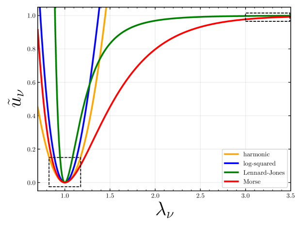
Figure 1: Shifted nondimensional scaled harmonic, log-squared, Lennard-Jones, and Morse segment potentials $\tilde{u}_{\nu}$ as a function of segment stretch $\lambda_{\nu}$. $\zeta_{\nu}^{char}=100$ for each potential, and $\kappa_{\nu}=1000$ for each potential (excluding the Lennard-Jones potential, where, by definition, $\kappa_{\nu}=72\zeta_{\nu}^{char}$).

3.2 Asymptotically matched segment behavior

3.2.1 Segment potential function

In order for the nondimensional chain force function $\xi_{c}(\lambda_{c}^{eq})$ as presented in Eq. 17 to truly be an analytical function of equilibrium chain stretch $\lambda_{c}^{eq}$, it is required that the segment stretch $\lambda_{\nu}$ also be an analytical function of $\lambda_{c}^{eq}$. The functional form of $\lambda_{\nu}$, defined as per Eq. 11, is dependent upon the complexity of the functional form of the segment potential $U_{\nu}(l_{\nu})$ and its first derivative. Several functional forms of $U_{\nu}(l_{\nu})$ have been proposed and utilized thus far in the literature, including the harmonic potential $U_{\nu}^{har}$ (mao2017large; mao2018theory; talamini2018progressive; li2020variational; mulderrig2021affine; arunachala2021energy; lamont2021rate), log-squared potential $U_{\nu}^{\ln^{2}}$ (mao2017rupture; arora2020fracture; arora2021coarse; xiao2021modeling; lu2020pseudo), Lennard-Jones potential $U_{\nu}^{lj}$ (jones1924determination; yang2020multiscale; zhao2021multiscale; feng2022rigorous; lei2022multiscale), and Morse potential $U_{\nu}^{morse}$ (morse1929diatomic; dal2009micro; buche2021chain; lavoie2019modeling; guo2021micromechanics):

$$U_{\nu}^{har}(l_{\nu})=E_{\nu}^{char}\left[\frac{1}{2}\frac{k_{\nu}}{E_{\nu}^{char}}\left[l_{\nu}-l_{\nu}^{eq}\right]^{2}-1\right],\qquad U_{\nu}^{\ln^{2}}(l_{\nu})=E_{\nu}^{char}\left[\frac{1}{2}\frac{[l_{\nu}^{eq}]^{2}k_{\nu}}{E_{\nu}^{char}}\left[\ln(\frac{l_{\nu}}{l_{\nu}^{eq}})\right]^{2}-1\right],$$ (22)

$$U_{\nu}^{lj}(l_{\nu})=E_{\nu}^{char}\left[\left[\frac{l_{\nu}^{eq}}{l_{\nu}}\right]^{12}-2\left[\frac{l_{\nu}^{eq}}{l_{\nu}}\right]^{6}\right],\qquad\qquad U_{\nu}^{morse}(l_{\nu})=E_{\nu}^{char}\left[\left[1-e^{-a_{\nu}[l_{\nu}-l_{\nu}^{eq}]}\right]^{2}-1\right],$$ (23)

where $a_{\nu}$ is the Morse parameter and is related to $E_{\nu}^{char}$ and $k_{\nu}$ via $k_{\nu}=2a_{\nu}^{2}E_{\nu}^{char}$. The nondimensional Morse parameter is defined as $\alpha_{\nu}\equiv l_{\nu}^{eq}a_{\nu}$. The nondimensional scaled segment potential $\overline{u}_{\nu}$, and its (non-negative) shifted counterpart $\tilde{u}_{\nu}$ are respectively defined as $\overline{u}_{\nu}\equiv u_{\nu}/\zeta_{\nu}^{char}$ and $\tilde{u}_{\nu}\equiv\overline{u}_{\nu}+1$. The proposed segment potentials from Eq. 22 and Eq. 23 are graphically presented in Fig. 1 (in $\tilde{u}_{\nu}$ form).

The harmonic potential is the simplest and most commonly used potential to account for segment extensibility, and it approximately captures the general behavior of the other potentials in a neighborhood of small $\lambda_{\nu}$ about the equilibrium state. However, for large $\lambda_{\nu}$, segment potentials are expected to escape the harmonic potential energy well and exhibit anharmonic behavior. By definition, only the log-squared, Lennard-Jones, and Morse potentials capture this behavior. Additionally, for large $\lambda_{\nu}$, segment potentials are expected to ultimately escape to an energy plateau equal to $E_{\nu}^{char}$. Only the Lennard-Jones and Morse potentials capture this behavior. To retain all of the characteristics of the ideal segment potential, we desire to use either the Lennard-Jones or Morse potential in the model framework to yield an analytical form for $\lambda_{\nu}$.

Unfortunately, due to the squared-exponential term in the Morse potential and two-term polynomial form of the Lennard-Jones potential, it is mathematically impossible for each of these potentials to lead to an approximate analytical expression for $\lambda_{\nu}$ as a function of $\lambda_{c}^{eq}$ as per Eq. 11 and Eq. 17 (where the inverse Langevin function involved with $\xi_{c}$ is represented by some approximant). In order to overcome this obstacle, we seek to derive a simple, quasi-polynomial segment potential which generally captures the essential aforementioned characteristics exhibited by the Lennard-Jones and Morse potentials. This derivation will necessarily evoke the principle of asymptotic matching, consistent to and allowing for integration within the $u$FJC framework. Using this derived segment potential, an expression for $\lambda_{\nu}$ as a function of $\lambda_{c}^{eq}$ will be reached.

To begin, consider the behavior of $\lambda_{\nu}$ in the low-to-intermediate chain force state as compared to that in the high chain force state. For low and intermediate chain forces, $\lambda_{\nu}$ resides in a neighborhood about the equilibrium state ($\lambda_{\nu}\approx 1$). The Lennard-Jones and Morse segment potentials in this neighborhood can be considered to be approximated via the harmonic potential (as highlighted by the black dashed box in the lower left of Fig. 1)

$$\tilde{u}_{\nu}(\lambda_{\nu})\approx\tilde{u}_{\nu}^{har}(\lambda_{\nu})=\frac{1}{2}\frac{\kappa_{\nu}}{\zeta_{\nu}^{char}}\left[\lambda_{\nu}-1\right]^{2}.$$ (24)

For high chain forces, $\lambda_{\nu}$ is large ($\lambda_{\nu}\gg 1$), and the Lennard-Jones and Morse segment potentials have reached their energy plateau equal to $E_{\nu}^{char}$ (as highlighted by the black dashed box in the upper right of Fig. 1)

$$\tilde{u}_{\nu}(\lambda_{\nu})\approx 1.$$ (25)

When naïvely applying Prandtl’s method of asymptotic matching to the above low-to-intermediate chain force and high chain force segment potentials (powers2015mathematical), it is self-evident that an asymptotically-matched composite potential is prohibited. To go about creating a simple, quasi-polynomial, and asymptotically-matched composite potential using the fundamental building blocks available to us in Eq. 24 and Eq. 25, we define a modulation parameter $\mu_{\nu}=\mu_{\nu}(\lambda_{\nu})$. $\mu_{\nu}$ is strictly a function of $\lambda_{\nu}$ with range $\mu_{\nu}\in[0,1]$. $\mu_{\nu}(\lambda_{\nu})$ is taken to be a monotonically-increasing function of $\lambda_{\nu}$. When $\mu_{\nu}=0$, the composite potential directly returns the harmonic potential ($\tilde{u}_{\nu}(\lambda_{\nu})=\frac{1}{2}\frac{\kappa_{\nu}}{\zeta_{\nu}^{char}}\left[\lambda_{\nu}-1\right]^{2}$), and when $\mu_{\nu}=1$, the composite potential directly returns the energy plateau $E_{\nu}^{char}$ ($\tilde{u}_{\nu}(\lambda_{\nu})=1$). Furthermore, $\mu_{\nu}\to 1$ faster than $\lambda_{\nu}\to\infty$, i.e., $\lim_{\lambda_{\nu}\to\infty}([1-\mu_{\nu}][\lambda_{\nu}-1])=0$. Finally, the overall composite potential $\tilde{u}_{\nu}(\mu_{\nu},\lambda_{\nu})$ is a monotonically-increasing function of $\lambda_{\nu}$ for $\lambda_{\nu}\geq 1$, as per Fig. 1. With all this taken into account, the low-to-intermediate chain force segment potential is modulated via $\mu_{\nu}$ as

$$\tilde{u}_{\nu}(\mu_{\nu},\lambda_{\nu})\approx[1-\mu_{\nu}]^{f}\tilde{u}_{\nu}^{har}(\lambda_{\nu})=[1-\mu_{\nu}]^{f}\frac{1}{2}\frac{\kappa_{\nu}}{\zeta_{\nu}^{char}}\left[\lambda_{\nu}-1\right]^{2},$$ (26)

and the high chain force segment potential is modulated via $\mu_{\nu}$ as

$$\tilde{u}_{\nu}(\mu_{\nu},\lambda_{\nu})\approx\mu_{\nu}^{g},$$ (27)

where $f$ and $g$ are integers. Now, we apply Prandtl’s method of asymptotic matching to the modulated low-to-intermediate chain force and high chain force segment potentials (powers2015mathematical), which involves satisfying

$$\lim_{\lambda_{\nu}\to\infty}[1-\mu_{\nu}]^{f}\frac{1}{2}\frac{\kappa_{\nu}}{\zeta_{\nu}^{char}}\left[\lambda_{\nu}-1\right]^{2}=\lim_{\lambda_{\nu}\to 0}\mu_{\nu}^{g}=0.$$ (28)

From the above, $f=2$ and $g\neq 0$ must hold true. In order to achieve the simplest composite function, we set $g=1$. The composite potential is consequentially written as

$$\tilde{u}_{\nu}(\mu_{\nu},\lambda_{\nu})=[1-\mu_{\nu}]^{2}\frac{1}{2}\frac{\kappa_{\nu}}{\zeta_{\nu}^{char}}[\lambda_{\nu}-1]^{2}+\mu_{\nu}.$$ (29)

All that remains to be satisfied is the condition that the composite potential is a monotonically-increasing function of $\lambda_{\nu}$ for $\lambda_{\nu}\geq 1$:

$$\partialderivative{\lambda_{\nu}}[\tilde{u}_{\nu}(\mu_{\nu},\lambda_{\nu})]=\partialderivative{\tilde{u}_{\nu}}{\mu_{\nu}}\partialderivative{\mu_{\nu}}{\lambda_{\nu}}+\partialderivative{\tilde{u}_{\nu}}{\lambda_{\nu}}\geq 0~{}\text{for}~{}\lambda_{\nu}\geq 1.$$ (30)

Since it is assumed that $\mu_{\nu}(\lambda_{\nu})$ is a monotonically-increasing function of $\lambda_{\nu}$, we seek to strongly satisfy the above by forcing the following equations to individually hold true

$$\partialderivative{\tilde{u}_{\nu}}{\lambda_{\nu}}=[1-\mu_{\nu}]^{2}\frac{\kappa_{\nu}}{\zeta_{\nu}^{char}}[\lambda_{\nu}-1]\geq 0~{}\text{for}~{}\lambda_{\nu}\geq 1,$$ (31)

$$\partialderivative{\tilde{u}_{\nu}}{\mu_{\nu}}=-[1-\mu_{\nu}]\frac{\kappa_{\nu}}{\zeta_{\nu}^{char}}[\lambda_{\nu}-1]^{2}+1\geq 0~{}\text{for}~{}\lambda_{\nu}\geq 1.$$ (32)

Using the properties of $\mu_{\nu}(\lambda_{\nu})$, Eq. 31 automatically holds true. The satisfaction of Eq. 32, as detailed in LABEL:app:modulation-parameter-definition, yields the functional form for $\mu_{\nu}=\mu_{\nu}(\lambda_{\nu})$:

$$\mu_{\nu}=\begin{cases}0,&\text{if~{}}\lambda_{\nu}<\lambda_{\nu}^{crit}\\ 1-\frac{\zeta_{\nu}^{char}}{\kappa_{\nu}\left[\lambda_{\nu}-1\right]^{2}},&\text{if~{}}\lambda_{\nu}\geq\lambda_{\nu}^{crit}\\ \end{cases},$$ (33)

where $\lambda_{\nu}^{crit}\equiv 1+\sqrt{\frac{\zeta_{\nu}^{char}}{\kappa_{\nu}}}$ is called the critical segment stretch (and $(\lambda_{c}^{eq})^{crit}$ is the corresponding critical equilibrium chain stretch).

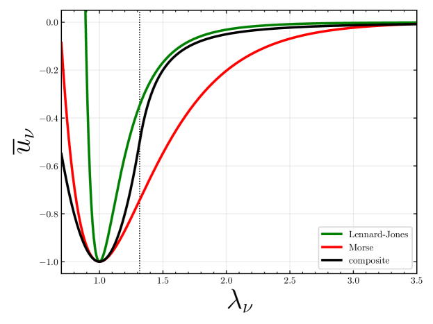
Figure 2: Lennard-Jones, Morse, and composite nondimensional scaled segment potentials $\overline{u}_{\nu}$ versus $\lambda_{\nu}$. The same $\zeta_{\nu}^{char}$ and $\kappa_{\nu}$ values are used here as in Fig. 1. The black dotted line denotes the critical segment stretch value $\lambda_{\nu}^{crit}$ for the composite segment potential.

With this, the composite nondimensional scaled segment potential $\overline{u}_{\nu}$ can be written as a function of $\lambda_{\nu}$

$$\overline{u}_{\nu}(\lambda_{\nu})=\begin{cases}\frac{1}{2}\frac{\kappa_{\nu}}{\zeta_{\nu}^{char}}[\lambda_{\nu}-1]^{2}-1,&\text{if~{}}\lambda_{\nu}<\lambda_{\nu}^{crit}\\ -\frac{\zeta_{\nu}^{char}}{2\kappa_{\nu}\left[\lambda_{\nu}-1\right]^{2}},&\text{if~{}}\lambda_{\nu}\geq\lambda_{\nu}^{crit}\\ \end{cases}.$$ (34)

The composite nondimensional segment potential $u_{\nu}$ is simply Eq. 34 multiplied by $\zeta_{\nu}^{char}$. Using the functional forms for the modulation parameter in Eq. 33 and the segment potential (e.g., Eq. 34), each presuppositional property of the modulation parameter $\mu_{\nu}$ and the composite segment potential $u_{\nu}$ can be trivially verified. Furthermore, it can also be verified that $u_{\nu}$ is continuous up to the first derivative at $\lambda_{\nu}=\lambda_{\nu}^{crit}$, i.e.,

$$u_{\nu}(\lambda_{\nu}^{crit})=-\frac{\zeta_{\nu}^{char}}{2}\text{~{}and~{}}\partialderivative{u_{\nu}}{\lambda_{\nu}}\bigg{|}_{\lambda_{\nu}=\lambda_{\nu}^{crit}}=\sqrt{\kappa_{\nu}\zeta_{\nu}^{char}}.$$ (35)

The composite $\overline{u}_{\nu}$ is plotted alongside its Lennard-Jones and Morse potential counterparts in Fig. 2. From this figure, it is clear that the composite potential exhibits the desired characteristics of the Lennard-Jones and Morse potentials: harmonic behavior near the equilibrium state and anharmonic behavior for large $\lambda_{\nu}$ tending to an energy plateau of $E_{\nu}^{char}$. These desired characteristics are expressed purely as a consequence of the derivation undertaken here, without any consideration of the specific functional form of the Lennard-Jones and Morse potentials. Conveniently, the derivation results in a composite potential with a simple functional form, as per Eq. 34.

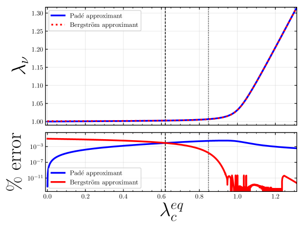
Figure 3: Segment stretch evolution prior to the critical chain state. Here, $\kappa_{\nu}=1000$, as per the composite segment potential displayed in Fig. 2. The black dashed line denotes the crossover equilibrium chain stretch $(\lambda_{c}^{eq})^{P2B}$. Additionally, the black dotted line denotes the equilibrium chain stretch $\lambda_{c}^{eq}$ value at which $\lambda_{c}^{eq}-\lambda_{\nu}+1=0.84136$. For $\lambda_{c}^{eq}$ values to the left of the black dotted line, $\lambda_{c}^{eq}-\lambda_{\nu}+1<0.84136$. (top) Segment stretch $\lambda_{\nu}$ as a function of $\lambda_{c}^{eq}$ in the domain $0\leq\lambda_{c}^{eq}<(\lambda_{c}^{eq})^{crit}$ using the Padé approximant from Eq. 40 and the Bergström approximant from Eq. 41. (bottom) Percent error of $\lambda_{\nu}$ in Eq. 40 and Eq. 41 relative to $\lambda_{\nu}$ calculated using a highly accurate numerical solution for the inverse Langevin function. (Beyond $\lambda_{c}^{eq}\approx 1$ the error in the Bergström approximant is sufficiently small such that its evaluation is dominated by floating-point error.)

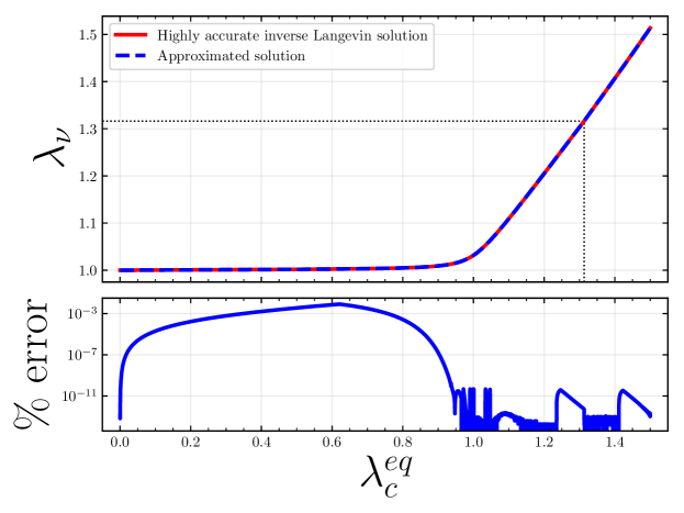
Figure 4: Segment stretch evolution. Here, $\zeta_{\nu}^{char}=100$ and $\kappa_{\nu}=1000$, as per the composite segment potential displayed in Fig. 2. The black dotted lines denote the critical equilibrium chain stretch $(\lambda_{c}^{eq})^{crit}$ and the critical segment stretch $\lambda_{\nu}^{crit}$. (top) Segment stretch $\lambda_{\nu}$ as a function of equilibrium chain stretch $\lambda_{c}^{eq}$ as per the approximated analytical $\lambda_{\nu}$ function from Eq. 43 along with $\lambda_{\nu}$ calculated using a highly accurate numerical solution for the inverse Langevin function. (bottom) Percent error of the approximated analytical $\lambda_{\nu}$ function in Eq. 43 relative to $\lambda_{\nu}$ calculated using a highly accurate numerical solution for the inverse Langevin function. (Beyond $\lambda_{c}^{eq}\approx 1$ the error in the approximated solution is sufficiently small such that its evaluation is dominated by floating-point error.)

3.2.2 Segment stretch function

With the simple, quasi-polynomial composite segment potential in hand, a highly accurate approximated analytical relationship between segment stretch and equilibrium chain stretch can now be derived. Substituting the composite $u_{\nu}$ (Eq. 34 multiplied by $\zeta_{\nu}^{char}$) into the definition of $\lambda_{\nu}$ in Eq. 11 and simplifying leads to

$$\xi_{c}=\mathcal{L}^{-1}(\lambda_{c}^{eq}-\lambda_{\nu}+1)=\partialderivative{u_{\nu}}{\lambda_{\nu}}=\begin{cases}\kappa_{\nu}[\lambda_{\nu}-1],&\text{if~{}}\lambda_{c}^{eq}<(\lambda_{c}^{eq})^{crit}\\ \frac{[\zeta_{\nu}^{char}]^{2}}{\kappa_{\nu}\left[\lambda_{\nu}-1\right]^{3}},&\text{if~{}}\lambda_{c}^{eq}\geq(\lambda_{c}^{eq})^{crit}\\ \end{cases}.$$ (36)

Note that $\lambda_{c}^{eq}<(\lambda_{c}^{eq})^{crit}$ corresponds one-to-one to the case when $\lambda_{\nu}<\lambda_{\nu}^{crit}$, and $\lambda_{c}^{eq}\geq(\lambda_{c}^{eq})^{crit}$ corresponds one-to-one to the case when $\lambda_{\nu}\geq\lambda_{\nu}^{crit}$. We now seek to employ an approximation for the inverse Langevin function in order to yield an approximate analytical solution. Two candidates stand out for the task: the Padé approximant (cohen1991pade)

$$\mathcal{L}^{-1}(y)\approxeq y\frac{3-y^{2}}{1-y^{2}},$$ (37)

and the Bergström approximant (bergstrom2000large)

$$\mathcal{L}^{-1}(y)\approxeq\frac{1}{\text{sgn}(y)-y},~{}\text{for~{}}0.84136<\absolutevalue{y}<1,$$ (38)

where $\text{sgn}(y)$ is the sign function:

$$\text{sgn}(y)=\begin{cases}-1,&\text{if~{}}y<0\\ 0,&\text{if~{}}y=0\\ 1,&\text{if~{}}y>0\\ \end{cases}.$$ (39)

Using the Padé approximant for the $\lambda_{c}^{eq}<(\lambda_{c}^{eq})^{crit}$ case and performing an appropriate cubic root analysis (zwillinger2002crc) leads to

$$\lambda_{\nu}=\lambda_{\nu}^{PSB}(\kappa_{\nu};\lambda_{c}^{eq}),$$ (40)

where the analytical form of $\lambda_{\nu}^{PSB}$ is provided in LABEL:app:analytical-form-segment-stretch-function. Likewise, using the Bergström approximant for the $\lambda_{c}^{eq}<(\lambda_{c}^{eq})^{crit}$ case and performing an appropriate quadratic root analysis leads to

$$\lambda_{\nu}=\lambda_{\nu}^{BSB}(\kappa_{\nu};\lambda_{c}^{eq}),$$ (41)

where the analytical form of $\lambda_{\nu}^{BSB}$ is provided in LABEL:app:analytical-form-segment-stretch-function.

The top panel in Fig. 3 displays $\lambda_{\nu}^{PSB}$ and $\lambda_{\nu}^{BSB}$ in the domain $0\leq\lambda_{c}^{eq}<(\lambda_{c}^{eq})^{crit}$, and the bottom panel displays the error of each approximation compared to $\lambda_{\nu}$ calculated using a highly accurate numerical solution for the inverse Langevin function. The bottom panel in Fig. 3 clearly shows that $\lambda_{\nu}^{PSB}$ is more accurate than $\lambda_{\nu}^{BSB}$ to the left of the black dashed line. On the contrary, $\lambda_{\nu}^{BSB}$ is more accurate than $\lambda_{\nu}^{PSB}$ to the right of the black dashed line. This black dashed line denotes $(\lambda_{c}^{eq})^{P2B}$, the equilibrium chain stretch value at which this crossover in numerical accuracy takes place (see Remarks 1 and 2 for more details).

Using the Bergström approximant for the $\lambda_{c}^{eq}\geq(\lambda_{c}^{eq})^{crit}$ case and performing an appropriate cubic root analysis (zwillinger2002crc) leads to

$$\lambda_{\nu}=\lambda_{\nu}^{BSP}(\zeta_{\nu}^{char},\kappa_{\nu};\lambda_{c}^{eq}),$$ (42)

where the analytical form of $\lambda_{\nu}^{BSP}$ is provided in LABEL:app:analytical-form-segment-stretch-function. Unfortunately, using the Padé approximant for the $\lambda_{c}^{eq}\geq(\lambda_{c}^{eq})^{crit}$ case results in a sixth-order polynomial in $\lambda_{\nu}$, which does not possess a general form for an analytical solution.

Considering all of this, the approximated analytical form of $\lambda_{\nu}$ as a function of $\lambda_{c}^{eq}$ is

$$\lambda_{\nu}=\begin{cases}\lambda_{\nu}^{PSB}(\kappa_{\nu};\lambda_{c}^{eq}),&\text{if~{}}\lambda_{c}^{eq}<(\lambda_{c}^{eq})^{P2B}\\ \lambda_{\nu}^{BSB}(\kappa_{\nu};\lambda_{c}^{eq}),&\text{if~{}}(\lambda_{c}^{eq})^{P2B}\leq\lambda_{c}^{eq}<(\lambda_{c}^{eq})^{crit}\\ \lambda_{\nu}^{BSP}(\zeta_{\nu}^{char},\kappa_{\nu};\lambda_{c}^{eq}),&\text{if~{}}\lambda_{c}^{eq}\geq(\lambda_{c}^{eq})^{crit}\end{cases}.$$ (43)

Fig. 4 displays the approximated $\lambda_{\nu}$ function as per Eq. 43, $\lambda_{\nu}$ calculated using a highly accurate numerical solution for the inverse Langevin function, and the percent error of the approximation. This figure convincingly verifies that the approximated analytical $\lambda_{\nu}$ function is highly accurate with respect to the highly accurate numerical solution in the domain of physically-sensible $\lambda_{c}^{eq}$.

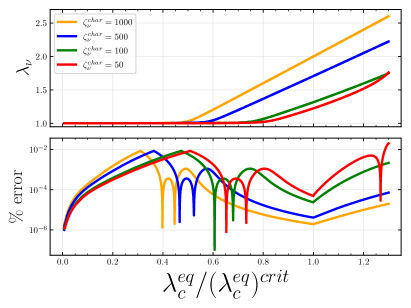
(a)

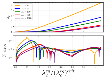
(b)

Figure 5: Comparison of segment stretches calculated via the $u$FJC chain force satisfaction method and the chain free energy minimization method. (a, top) Segment stretch $\lambda_{\nu}$ calculated via the $u$FJC chain force satisfaction method as a function of equilibrium chain stretch normalized by the critical equilibrium chain stretch, $\lambda_{c}^{eq}/(\lambda_{c}^{eq})^{crit}$, for $\kappa_{\nu}=1000$ and varying $\zeta_{\nu}^{char}$. (b, top) $\lambda_{\nu}$ calculated via the $u$FJC chain force satisfaction method as a function of $\lambda_{c}^{eq}/(\lambda_{c}^{eq})^{crit}$, for $\zeta_{\nu}^{char}=100$ and varying $\kappa_{\nu}$. (bottom) Percent error of $\lambda_{\nu}$ calculated via the chain free energy minimization method (with respect to $\lambda_{\nu}$ calculated via the $u$FJC chain force satisfaction method) as a function of $\lambda_{c}^{eq}/(\lambda_{c}^{eq})^{crit}$. The sharp dips in these percent error curves take place where the $\lambda_{\nu}$ values calculated by the chain free energy minimization method cross over or under the $\lambda_{\nu}$ values calculated by the $u$FJC chain force satisfaction method.

In accordance with the $u$FJC model framework as introduced in buche2021chain and buche2022freely (the reader is referred to the arguments detailed therein), $\lambda_{\nu}$ is implicitly defined to satisfy the equality between the chain force and the segment force, as per Eq. 11. This $u$FJC chain force satisfaction method differs from the condition that $\lambda_{\nu}$ be the minimizer of the chain Helmholtz free energy $\Psi_{c}$, as proposed by mao2017rupture and widely adopted in the literature since:

$$\lambda_{\nu}=\operatorname*{arg\,min}_{\lambda_{\nu}\geq 1}\hat{\Psi}_{c}(\lambda_{\nu}),\text{~{}where~{}}\hat{\Psi}_{c}(\lambda_{\nu})=\Psi_{c}(\lambda_{\nu},\lambda_{c}=\hat{\lambda}_{c}),$$ (44)

where $\lambda_{c}=\hat{\lambda}_{c}$ is a given imposed chain stretch.

In an effort to compare the numerical results of the chain free energy minimization method to the $u$FJC chain force satisfaction method, $\lambda_{\nu}$ is calculated via both methods for increasingly steep segments, with the latter method presented in the top panels in Fig. 5. The percent error of the $\lambda_{\nu}$ calculation from the chain free energy minimization method (with respect to the $u$FJC chain force satisfaction method) is provided in the bottom panels. In order to ensure an equal comparison between both $\lambda_{\nu}$ calculation methods, $\Psi_{c}$ involved in the chain free energy minimization method obeys Eq. 20 multiplied by $\nu/\beta$. In addition, $\lambda_{\nu}$ is presented as a function of $\lambda_{c}^{eq}$, which normalizes the impact of chain segment number on the $\lambda_{\nu}$ calculations. $\lambda_{c}^{eq}$ is then further divided by $(\lambda_{c}^{eq})^{crit}$ as a means of normalizing the impact of differing $(\lambda_{c}^{eq})^{crit}$ values for segments with varying $\zeta_{\nu}^{char}$ and $\kappa_{\nu}$. As indicated by the bottom panels in Fig. 5, the chain free energy minimization method numerically complies quite well with the $u$FJC chain force satisfaction method for $\lambda_{c}^{eq}$ less than, equal to, and slightly greater than $(\lambda_{c}^{eq})^{crit}$, i.e., for low and intermediate chain forces $\xi_{c}$. For extremely large $\lambda_{c}^{eq}$, i.e., for extremely high chain forces $\xi_{c}$, the chain free energy minimization method will numerically diverge from the $u$FJC chain force satisfaction method. This is implied by the trend in the percent error curves for increasing $\lambda_{c}^{eq}/(\lambda_{c}^{eq})^{crit}\gg 1$.

Remark 1.

The black dashed line in Fig. 3 denotes $(\lambda_{c}^{eq})^{P2B}$, the equilibrium chain stretch value at which the Padé approximant $\lambda_{\nu}$ solution becomes less numerically accurate than the Bergström approximant $\lambda_{\nu}$ solution (hence $P2B$). Given Eq. 40 and Eq. 41, $(\lambda_{c}^{eq})^{P2B}$ solely depends on $\kappa_{\nu}$. A curve fit analysis was used to determine the relationship between $(\lambda_{c}^{eq})^{P2B}$ and $\kappa_{\nu}$:

$$(\lambda_{c}^{eq})^{P2B}=\frac{1}{\kappa_{\nu}^{n}}+b,\text{~{}where~{}}n=0.8187\text{~{}and~{}}b=0.6176.$$ (45)