Chen, Golrezaei and Susan

Fair Assortment Planning

Fair Assortment Planning

Qinyi Chen Operations Research Center, Massachusetts Institute of Technology, Cambridge, MA 02139, qinyic@mit.edu Negin Golrezaei Sloan School of Management, Massachusetts Institute of Technology, Cambridge, MA 02139, golrezae@mit.edu Fransisca Susan Operations Research Center, Massachusetts Institute of Technology, Cambridge, MA 02139, fsusan@mit.edu

Many online platforms, ranging from online retail stores to social media platforms, employ algorithms to optimize their offered assortment of items (e.g., products and contents). These algorithms tend to prioritize the platforms’ short-term goals by solely featuring items with the highest popularity or revenue. However, this practice can then lead to undesirable outcomes for the rest of the items, making them leave the platform, and in turn hurting the platform’s long-term goals. Motivated by that, we introduce and study a fair assortment planning problem, which requires any two items with similar quality/merits to be offered similar outcomes. We show that the problem can be formulated as a linear program (LP), called (fair), that optimizes over the distribution of all feasible assortments. To find a near-optimal solution to (fair), we propose a framework based on the Ellipsoid method, which requires a polynomial-time separation oracle to the dual of the LP. We show that finding an optimal separation oracle to the dual problem is an NP-complete problem, and hence we propose a series of approximate separation oracles, which then result in a $1/2$-approx. algorithm and a PTAS for the original Problem (fair). The approximate separation oracles are designed by (i) showing the separation oracle to the dual of the LP is equivalent to solving an infinite series of parameterized knapsack problems, and (ii) taking advantage of the structure of the parameterized knapsack problems. Finally, we conduct a case study using the MovieLens dataset, which demonstrates the efficacy of our algorithms and further sheds light on the price of fairness.

assortment planning, fairness, online platforms, approximation algorithm, customer exposure

1 Introduction

Algorithms have been extensively used by modern online platforms, such as online retail stores and social media platforms, to optimize their operational decisions, ranging from assortment planning (e.g., Kok et al. (2008), Rusmevichientong et al. (2010), Davis et al. (2014), Golrezaei et al. (2014)) to pricing (e.g., Derakhshan et al. (2019), Cohen et al. (2020), Golrezaei et al. (2021a)) to product ranking (e.g., Derakhshan et al. (2020), Golrezaei et al. (2021b), Niazadeh et al. (2021)) to resource allocation (Mehta et al. (2007), Golrezaei and Yao (2021), Gorlezaei et al. (2022)). While the use of algorithms can make the decision-making processes more efficient, they can also create unfair environments for some of the crucial players of the online platforms. In assortment planning, for example, single-minded algorithms that are only concerned about the platforms’ short-term objective (e.g., revenue or market share) can treat some of the items (e.g., products on online retail stores; posts on social media) on the platforms unfairly. Algorithms that prioritize only the most popular or profitable items in an assortment can lead to undesirable outcomes for the rest of the items, such as limited visibility and revenue. As a result, the sellers or content creators of these items may become dissatisfied and even choose to leave the platform, creating an unhealthy ecosystem with negative long-term consequences for the platform. This raises the following research question: How can we design fair assortment planning algorithms under which any two items with similar merits get similar outcomes?

As alluded earlier, answering the question above can be of interest to a number of online platforms, such as online retail stores, social media platforms, job search sites, movie/music recommendation sites, to name a few. In all of these online platforms, a “winner-take-all” phenomenon can become prevalent due to the wide adoption of algorithmic recommendations:

• In online retail stores like Amazon, the platform often features the most popular or profitable products (e.g., as “Amazon’s Choices”), or those produced by Amazon’s own label (Amazon Basics), while relegating products with similar ratings and prices to subsequent pages. This can make it challenging for less popular products or those produced by local sellers to attract visibility, since most Amazon customers rarely scroll past the first page of search results (Search Engine Journal 2018). The European Parliament is recently attempting to address this through the Digital Market Act (Official Journal of the European Union 2023), which seeks to promote fairness by banning large platforms from ranking their own products more favorably than third-party sellers (CNBC 2022).

• Social media platforms like Instagram is widely adopted by business owners for marketing purposes. However, the recommendation algorithms used by Instagram tend to mostly prioritize high-quality social media posts made with special camera effects, while many small businesses lack necessary video-editing equipment and skills. This then leads to an unfair outcome where small business owners have seen a notable decrease in the amount of user engagement on their posts, as well as in the number of their sales (The New York Times 2022b).

• On job search sites such as LinkedIn, the items correspond to users who network with each other and search for job openings. By design of their algorithm, active users tend to be connected to other users or job postings more frequently, due to their greater representation in the data collected (VentureBeat 2021). However, this creates an unfair environment where the most active users keep expanding their network, while the less active users get very little visibility among other users or recruiters.

• Finally, the algorithms used by many movie/music recommendation sites are self-reinforcing and the cultural products they recommend to a specific user are often restricted to a few genres or types (Vox 2019). This raises the concern that certain cultural products might not survive the algorithms since they do not get sufficient exposure among the audience.

All of the examples above demonstrate the practical importance of taking fairness into account while performing assortment planning for different types of items on a variety of online platforms.

1.1 Our Contributions

Fair assortment planning problem. To address the aforementioned research question, we consider an online platform that hosts $n$ items, which can represent products, social media posts, job candidates, movies/music in corresponding contexts. Each item $i$ has a popularity weight $w_{i}>0$ that is a proxy for the item $i$’s popularity. If purchased/chosen by the user, item $i$ also generates some revenue $r_{i}\in(0,\bar{r}]$, which is the monetary value that the platform earns when the user chooses item $i$. The platform’s goal is to maximize its expected revenue or market share by optimizing its offered assortment, which consists of at most $K$ items, for its users. The users choose an item according to the multinomial choice model with popularity weight $w_{i}$, $i\in[n]$.

We would like to ensure a fair environment for all items on the platform. To achieve this, we introduce a parameterized notion of fairness that is based on the parity of pairwise normalized outcome across items. The term outcome can represent a range of metrics that the items value, such as visibility, market share, expected revenue, or weighted combinations thereof. The normalized outcome of an item is defined as its outcome divided by its quality/relevance score. The quality score of an item $i$ can be a function of its weight and revenue, as well as other factors such as its relevance to search results, consumer ratings, etc.

To ensure a fair ecosystem, the platform aims to make the normalized outcomes of all items comparable. This allows for a standardized comparison of outcomes, independent of the varying quality levels of different items. By doing so, we can promote fairness and equal opportunities for all items on the platform. While assortment planning problems with different objective functions have been widely studied (see Kok et al. (2008) for a survey), prior to this work, enforcing fairness in assortment planning problems has not been studied in the literature.

Our fairness notion. We briefly comment on our fairness notion, which is formally defined in Section 3. One of the major challenges in defining and enforcing fairness for items is the conflicting interests among different stakeholders, such as the platform and its items. To illustrate this challenge, let us consider traditional fairness notions, such as the notion of alpha fairness (Mo and Walrand 2000, Lan et al. 2010), which includes the Nash bargaining solution (Nash Jr 1950). In such notions, the platform considers an aggregate function that maps the vector of items’ outcomes or utilities to social welfare, which is a scalar. The platform then aims to maximize the social welfare. However, the platform’s revenue is either ignored or can be incorporated into the social welfare, treating the platform as one of the items. This creates a conflict of interests since the platform aims to maximize its revenue, while the fairness notion aims to maximize the social welfare of all items.

Enforcing fairness in practice would hence require careful consideration of such conflicting interests and finding a balance that satisfies all stakeholders. To address this, we propose introducing fairness as constraints in a constrained optimization problem. In this optimization problem, the platform maximizes its revenue while ensuring fairness for all items. The level of fairness can be flexibly adjusted by tuning a parameter. Please refer to Section 4 for a comprehensive discussion of our fairness notion.

Fair Ellipsoid-based assortment planning algorithms. In Section 5, we first show that there exists an optimal solution to the aforementioned fair assortment planning problem that randomizes over at most $\mathcal{O}(n^{2})$ assortments (Theorem 5.1), making the implementation of the optimal solution practically feasible. We then present a framework that provides a wide range of near-optimal algorithms for the fair assortment planning problem, denoted by Problem (fair).

Our framework uses the Ellipsoid method and a (near-)optimal polynomial-time separation oracle to the dual counterpart of the fair assortment planning problem, denoted by Problem (fair-dual). Ideally, the Ellipsoid method would require an optimal separation oracle for Problem (fair-dual), where the separation oracle would either declare a point is feasible or return a hyperplane that separates the point from the convex set that describes the feasible region. We show that while designing a polynomial-time optimal separation oracle for Problem (fair-dual) is possible for certain problem instances (where the outcome received by an item is its revenue or market share), it remains an NP-complete problem for general instances (see Theorem 5.2). However, we establish that even if a $\beta$-approximate separation oracle for Problem (fair-dual) can be created, it is possible to construct a $\beta$-approximate solution to Problem (fair) using the Ellipsoid method, where $\beta\in(0,1]$; refer to Theorem 5.3 for more details.

Separation oracle as solving an infinite number of knapsack problems. Having established this result (Theorem 5.3), we then proceed to design near-optimal separation oracles for Problem (fair-dual) under general instances. To do so, we show that we need to find a set $S$ with a cardinality of at most $K$ that maximizes a cost-adjusted revenue, where the costs are functions of dual variables associated with the fairness constraints. To solve this problem, we take advantage of a novel transformation that shows maximizing cost-adjusted revenue is equivalent to solving an infinite series of knapsack problems with both cardinality and capacity constraints (see Theorem 6.2). Each knapsack problem is parameterized by its capacity $W\in[0,\infty)$, where parameter $W$ also influences the utility of items: the larger the $W$, the smaller the utilities. Given this transformation, we then design a series of polynomial-time, $\beta$-approximate algorithms for solving these infinite knapsack problems. Together with the Ellipsoid method, these then give rise to a series of $\beta$-approximate fair Ellipsoid-based algorithms for the original Problem (fair).

$1/2$-approx. separation oracle. In Section 7, we first present an polynomial-time $1/2$-approx. algorithm (Algorithm 1 and Theorem 7.3) for the infinite series of parameterized knapsack problems, which then result in a $1/2$-approx. separation oracle for Problem (fair-dual). We first note that for each one of the aforementioned knapsack problems, a $1/2$-approx. solution can be obtained using the profile associated with the optimal basic solution to the LP relaxation of the knapsack problem, where a profile determines the set of items that are fully added, fractionally added, and not added to the knapsack at the optimal solution (Caprara et al. 2000). However, while solving one relaxed knapsack problem is doable in polynomial time, we cannot possibly solve an infinite number of them in order to find the corresponding approximate solutions. A key observation here is that while the 1/2-approx. solutions can vary as the parameter of the knapsack increases, their associated profiles undergo at most $\mathcal{O}(nK)$ number of changes. This then allows us to maintain a polynomial-size collection of sets that contains a 1/2-approx. solution to the infinite series of parameterized knapsack problems. To maintain this collection, which is one of the most important steps of our algorithm, we determine the points at which the profile changes dynamically, and once a change point is detected, we update the profile using a simple rule that takes advantage of the structure of the parameterized knapsack problems.

PTAS separation oracle. In Section 8, with the help of our $1/2$-approx. algorithm presented in Algorithm 1, we then present a polynomial-time approximation scheme (PTAS) for the infinite series of parameterized knapsack problems in Algorithm 2, which returns an $(1-\epsilon)$-approximate solution in time polynomial in $n$ and $K$, for any accuracy parameter $\epsilon>0$. As discussed previously, this results in a PTAS separation oracle for Problem (fair-dual), which in turn gives rise to a PTAS fair Ellipsoid-based algorithm for Problem (fair). The PTAS iterates through two types of sets: (1) all of the small-sized sets and (2) large-sized sets that potentially have high utilities. In particular, to construct the large-sized sets with high utilities, we crucially rely on our $1/2$-approx. algorithm stated above. See Algorithm 2 and Theorem 8.1.

Connection between the separation oracles and the assortment optimization problem with fixed costs. In our Ellipsoid-based framework, to design separation oracles, we are tasked with finding a set $S$ with a maximum cardinality of $K$ that maximizes the cost-adjusted revenue. To solve this problem, as stated above, we cast it as an infinite series of knapsack problems and have developed near-optimal algorithms. These algorithms are also applicable to the capacitated assortment optimization problem with fixed costs, where the objective is to find a set with a maximum cardinality of $K$ that maximizes revenue minus production/display costs. This problem can be of interest to readers. A simpler version of this problem, without the cardinality constraints, has been studied in Kunnumkal et al. (2010). However, introducing the cardinality constraints significantly increases the complexity of the problem and demands new ideas.

Numerical studies on real-world/synthetic data and managerial insights. We numerically evaluate the performance of our near-optimal algorithms ($1/2$-approx. algorithm and PTAS) on both real-world and synthetic datasets. In Section 9, we consider a real-world movie recommendation setting based on the MovieLens dataset. Our case study examines the price of fairness (i.e., the loss in market share due to enforcing fairness constraints), as well as the impact of fairness constraints on sellers’ visibility. In Section 16, we further evaluate the performance of our algorithms in a number of synthetically generated, yet real-world inspired instances.

Our numerical studies show that the $1/2$-approx. algorithm is a practical option that produces solutions of comparable quality to the PTAS while achieving superior runtime performance. From a managerial perspective, our results provide insights into how fairness can be effectively enforced on online platforms at minimal cost, particularly in cases such as movie recommendations where item quality is similar. Our methods demonstrate the ability to generate high-performing solutions that effectively balance the platform’s revenue maximization goals with the need for fairness across all items. Furthermore, we also observe that implementing these solutions requires minimal effort from the platform’s side, as most near-optimal solutions only require randomization of a small number of assortments. By enforcing fairness constraints, online ecosystems can achieve long-term sustainability, offsetting the small short-term cost of fairness.

Proofs of all analytical results presented in this paper are included in the appendix.

2 Related Work

Fairness in supervised learning. With the increasing penetration of machine learning algorithms, there has been an explosion of work on algorithmic fairness in supervised learning, especially binary classification and risk assessment (Calders et al. (2009), Dwork et al. (2012), Hardt et al. (2016), Goel et al. (2018), Ustun et al. (2019)). Generally, the definitions of algorithmic fairness fall under three different types: (i) individual fairness, where similar individuals get similar predictions (Dwork et al. (2012), Kusner et al. (2017), Loi et al. (2019)), (ii) group fairness, where different groups are treated equally (Calders et al. (2009), Zliobaite (2015), Hardt et al. (2016)), and (iii) subgroup fairness, which combines individual and group notions of fairness (Kearns et al. (2018), Kearns et al. (2019)). Roughly speaking, in our setting, we consider individual fairness for each of the sellers on the online platform. However, our work is different from the aforementioned works because we do not study a prediction problem using labeled data (as they do), but instead we look into an optimization problem (assortment optimization) while imposing fairness constraints.

Fairness in resource allocation. At a high level, in our problem, an online platform would like to allocate exposure (an intangible resource) to different items in a fair fashion while optimizing for customers’ satisfaction. Having this view in mind, there are works that study fair resource allocation problems for more tangible resources. These works can be divided into two streams.

The first stream considers static settings where the resource allocation needs to be done in a single shot, and studies the trade-off between fairness and efficiency Bertsimas et al. (2011), Bertsimas et al. (2012), Hooker and Williams (2012), Donahue and Kleinberg (2020)). See also Cohen et al. (2021a) for a recent work that studies fairness in price discrimination in a static setting and Deng et al. (2022) that studies fairness and more specifically individual welfare in auctions run in search advertising markets.

The second stream investigates dynamic settings, where resources should be allocated over time. See Manshadi et al. (2021) for fairness in an online scarce resource allocation problem with correlated demands, Balseiro et al. (2021), Bateni et al. (2021) for regularized fair online resource allocation problems, Ma et al. (2021) for fairness in online matching, Sinclair et al. (2021) for fair sequential allocation that achieves the optimal envy-efficiency trade-off, Mulvany and Randhawa (2021) for fairness in scheduling, Baek and Farias (2021) for fairness in bandit setting, Schoeffer et al. (2022) for fairness in the spread of contents, and Aminian et al. (2023) for fairness in Markovian search. Our work is closer to the works in the first stream, rather the second one. That being said, we are the first one that studies fairness in an assortment planning problem.

Fairness in ranking. Our work is also related to the literature on fairness in ranking, where the goal is to optimize over the permutations of items displayed to users. (See Patro et al. (2022) for a survey.) We can view our assortment planning problem as a special case of ranking problem where the items placed in the top $K$ positions are chosen in the assortment, while the rest of the items are not chosen. Within this literature, Singh and Joachims (2018), Biega et al. (2018), Singh and Joachims (2019) are three works that are the most similar to ours in the sense that they oppose the “winner-take-all” allocation of economic opportunity.

Similar to our work, these studies aim to achieve proportional exposure/visibility for each item based on its relevance/quality. Since the nature of both ranking and assortment planning problems is combinatorial, designing an efficient algorithm is challenging. Singh and Joachims (2018) overcome this by considering distribution over rankings and imposing that the expected utility is linear in terms of both (i) attention an item gets at a certain position, and (ii) utility value of each item for each type of user. Biega et al. (2018) look at a dynamic setting that involves a number of rounds of decision-making. At each round, they use an integer LP to find the ranking that minimizes cumulative measure of unfairness, given all of the previous rankings. Singh and Joachims (2019) try to learn a fair ranking using a policy-gradient approach that maximizes utility while minimizing group fairness disparity. Neither Biega et al. (2018) nor Singh and Joachims (2019) provide theoretical guarantees. In contrast, our work presents algorithms with provable performance guarantees. We further believe our fairness notion and mathematical framework can be easily extended to a product ranking setting.

3 Model

In this section, we provide details on our model and formulate the platform’s optimization problem.

3.1 User’s Choice Models

We consider a platform with $n$ items, indexed by $i\in[n]$. Each item $i$ has a weight $w_{i}\geq 0$ that measures how popular the item is to the platform’s users. Upon offering an assortment/set $S$ of items, the users purchase/choose item $i\in S$ according to the MNL model (Train (1986)), with probability $\frac{w_{i}}{1+w(S)}\,,$ where $w(S)=\sum_{i\in S}w_{i}$. The users may also choose not to purchase any item with probability $\frac{1}{1+w(S)}$; that is, the no-purchase option (item $0$) is always included in set $S$. If item $i$ is purchased by the users, it generates revenue $r_{i}\in(0,\bar{r}]$. The action of purchasing an item can be viewed as “taking the desired action” under different contexts (e.g., purchasing a product in an online retail store, clicking on a post on a social media platform, or watching a movie on a movie recommendation site).

The main objective of the platform is to optimize over its offered assortment that can contain at most $K$ items in order to maximize its expected revenue, which we denote as

$$\textsc{rev}(S)=\frac{\sum_{i\in S}r_{i}w_{i}}{1+w(S)}\,.$$

For online platforms such as social media or job recommendation sites where there is no revenue associated with each item, we can assume revenue $r_{i}=1$ for any $i\in[n]$. With these revenue values, maximizing $\textsc{rev}(\cdot)$ is equivalent to maximizing the platform’s market share (or users’ engagement), i.e., the probability that users select an item from the offered assortment, which is another commonly adopted platform’s objective (see Wang and Sahin (2018), Derakhshan et al. (2020), Golrezaei et al. (2021b), Niazadeh et al. (2021) for some works that consider such objectives). It is worth noting that the uniform revenue setting can be useful for platforms aiming to maximize market share or using a fixed commission model. It can also lead to algorithms with better runtime in some problem instances; see Sections 14.1 and 15.

3.2 Fairness Notions

The platform is also interested in providing a fair marketplace for all of the items on the platform. In particular, the platform would like to ensure that any two items with similar quality (which will be defined shortly) receive a fair allocation of outcomes.

We let $O_{i}(S)$ denote the outcome received by item $i$ upon offering set $S$ and, with a slight abuse of notation, let $O_{i}=\sum_{S:i\in S}O_{i}(S)p(S)$ be the expected outcome of item $i$, where the outcome of item under set $S$ takes the following general form:

$$O_{i}(S)=a_{i}\cdot\frac{w_{i}}{1+w(S)}+b_{i}$$ (1)

for some $a_{i},b_{i}\geq 0$. In the following, we discuss some special cases of outcomes that fit Equation (1). Our definition of outcome gives us the flexibility to consider any of the following metrics or any weighted combinations of them as the outcome of item $i$.

• Visibility ($a_{i}=0,b_{i}=1$). Here, $O_{i}=\sum_{S:i\in S}p(S)$ is the probability that item $i$ is shown to a user. We refer to this as visibility or user exposure.

• Revenue ($a_{i}=r_{i},b_{i}=0$). Here, $O_{i}(S)=r_{i}\cdot\frac{w_{i}}{1+w(S)}$ is the expected revenue generated by sale of item $i$ under set $S$. Under a percentage commission model, $O_{i}=\sum_{S:i\in S}O_{i}(S)p(S)$ is proportional to the revenue earned by item $i$.

• Market share ($a_{i}=1,b_{i}=0$). Here, $O_{i}(S)=\frac{w_{i}}{1+w(S)}$ is the expected market share of item $i$ under set $S$.

We remark that the outcome received by item $i$ can be interpreted differently under different contexts. For example, content creators on streaming platforms often care more about the visibility of their contents, while sellers on online marketplaces might be more concerned about their revenues/profits. Nonetheless, as stated above, any weighted combination of visibility, revenue, and market share can be used an outcome for the items.

To ensure a fair ecosystem, the platform aims to ensure that the normalized outcomes of all items are comparable. The normalized outcome of an item $i$ is determined by dividing its outcome by its quality score, where this ratio allows for a standardized comparison of outcomes, independent of the varying quality levels of different items. The platform measures the quality of item $i$ using some non-negative, rational function $q_{i}(w_{i},r_{i})\geq 0$, which can depend on the popularity weight $w_{i}$, revenue $r_{i}$, as well as, other features of the item.

We assume that the function $q_{i}(.)$ is known, but can take any arbitrary form (one example is $q_{i}(w_{i},r_{i})=g_{i}(w_{i})+h_{i}(r_{i})$, where $g_{i}(.)$ and $h_{i}(.)$ are increasing functions). The quality function $q_{i}(.)$ also does not need to rely solely on the weight and revenue of item $i$, but can additionally capture the item’s relevance to the search results, consumer ratings, etc. The platform can use any method of its choice to measure an item’s quality, such as past data on returns, reviews, and market surveys. Our framework can flexibly handle any quality function $q_{i}(.)$ regardless of how it is measured. Throughout the rest of this paper, to ease the exposition, we suppress the dependency of $q_{i}(w_{i},r_{i})$ on $w_{i}$ and $r_{i}$, and use $q_{i}$ to denote the quality/merit of item $i$.

Having both the quality and outcome of items in mind, the platform now considers a parameterized notion of fairness that is based on the parity of pairwise normalized outcome across different items. We say that the platform is $\delta$-fair if, for any pair of items $(i,j)$, we have

$$\frac{O_{i}}{q_{i}}-\frac{O_{j}}{q_{j}}\leq\delta\qquad\Longleftrightarrow\qquad q_{j}\cdot\sum_{S:i\in S}O_{i}(S)p(S)-q_{i}\cdot\sum_{S:j\in S}O_{j}(S)p(S)\leq\delta\cdot q_{i}q_{j}\qquad\text{$i,j\in[n]$}\,.$$ (2)

Here, $\frac{O_{i}}{q_{i}}$ is a normalized outcome received by item $i$, scaled by its quality measure.

Pairwise notions of fairness are quite common in the literature and have been used in various settings, including recommendation systems (Beutel et al. 2019), ranking and regression models (Narasimhan et al. 2020, Kuhlman et al. 2019, Singh et al. 2021), and predictive risk scores (Kallus and Zhou 2019). Our approach to achieving pairwise fairness with respect to normalized outcome is closely related to the fairness notion employed in Biega et al. (2018), Singh and Joachims (2019), Schoeffer et al. (2022) for ranking problems, which, similar to our setting, seeks to allocate visibility in proportion to item quality. However, our formulation of pairwise fairness in the assortment planning setting is a novel contribution not explored in prior works. See Section 4 for an extended discussion on our fairness notions and its comparison with prior notions in the economic literature. We additionally note that our generic definitions above allow us to have a flexible framework in which the platform can be fair with respect to any quality measure and any outcome of its choice (not only visibility); see Section 4.2.

Note that as parameter $\delta$ in Equation (2) increases, the platform gets less concerned about being fair toward the items. When $\delta=0$ (i.e., when the platform is $0$-fair), the above constraint can be written as $\frac{O_{i}}{q_{i}}=\frac{O_{j}}{q_{j}}$. That is, the outcome received by item $i$ is exactly proportional to its quality. For any $\delta\geq\frac{\max_{i\in[n]}O_{i}}{\min_{i\in[n]}q_{i}}$, the fairness constraint is simply satisfied at the optimal solution in the absence of the fairness constraint, i.e., by always offering the single assortment with the largest expected revenue. While the optimal solution without fairness constraints maximizes platform’s expected revenue, it can lead to a very unfair outcome when the quality of some items that are not included in the offered assortment are close to, or even exceed the quality of those included.

3.3 Platform’s Objective

Having defined the user’s choice model and the fairness notion, we define an instance of our fair assortment planning problem using $\Theta=(\textbf{a},\textbf{b},\textbf{r},\textbf{w},\textbf{q})\in\mathbb{R}_{+}^{5n}$, where $\textbf{a}=\{a_{i}\}_{i\in[n]}$ and $\textbf{b}=\{b_{i}\}_{i\in[n]}$ determine outcomes of items (see Equation 1), $\textbf{r}=\{r_{i}\}_{i\in[n]}$ represents item revenues, $\textbf{w}=\{w_{i}\}_{i\in[n]}$ represents item weights, and $\textbf{q}=\{q_{i}\}_{i\in[n]}$ represent item qualities. We now define two specific instances of our problem.

• Revenue/Marketshare-Fair Instance. We call an instance with the form $\Theta=(\textbf{a},0,\textbf{r},\textbf{w},\textbf{q})$ a revenue/marketshare-fair instance. Here, the outcome of item $i$ upon presenting it in set $S$ is $O_{i}(S)=a_{i}\cdot\frac{w_{i}}{1+w(S)}$, which is either item $i$’s revenue when $a_{i}=r_{i}$ or item $i$’s market share when $a_{i}=1$.

• Visibility-Fair Instance. We call an instance with the form $\Theta=(0,\textbf{b},\textbf{r},\textbf{w},\textbf{q})$ a visibility-fair instance. Here, the expected outcome received by item $i$ is $O_{i}=b_{i}\cdot\sum_{S:i\in S}p(S)$, which is proportional to the probability that item $i$ is shown to a user (i.e., the visibility of item $i$).

While our algorithms can be applied to Problem (fair) for any instance $\Theta\in\mathbb{R}_{+}^{5n}$, better results can be achieved for the revenue/marketshare-fair and visibility-fair instances. Specifically, we will prove that there exists a polynomial-time optimal algorithm for Problem (fair) for any revenue/marketshare-fair instance. On the other hand, the visibility-fair instance poses more significant challenges and demands near-optimal solutions. Nevertheless, when item revenues are homogeneous, it is possible to devise near-optimal algorithms with low time complexity; see Sections 14.1 and 15 for further details.

Given any instance $\Theta\in\mathbb{R}_{+}^{5n}$, the platform wishes to maximize its expected revenue by optimizing over its offered assortment with cardinality of at most $K$, subject to the fairness constraints in Equation (2). This gives the platform’s optimization problem:

$$\textsc{fair}~{}=~{}\max_{p(S)\geq 0:S\subseteq[n]} \sum_{S:|S|\leq K}p(S)\cdot\textsc{rev}(S)$$

s.t. $$\quad q_{j}\cdot\sum_{S:i\in S}O_{i}(S)p(S)-q_{i}\cdot\sum_{S:j\in S}O_{j}(S)p(S)\leq\delta\cdot q_{i}q_{j}\quad\quad~{}~{}~{}~{}~{}i,j\in[n],i\neq j$$

$$\sum_{S:|S|\leq K}p(S)\leq 1\,,$$ (fair)

where $\textsc{rev}(S)=\frac{\sum_{i\in S}r_{i}w_{i}}{1+w(S)}$ is the platform’s expected revenue upon offering assortment $S\subseteq[n]$. Here, we slightly abuse the notation and denote both the platform’s problem and the optimal expected revenue with the term fair. In Problem (fair), the objective is the platform’s expected revenue. The first set of constraints is the fairness constraints, and the second constraint enforces $\{p(S)\}_{S:|S|\leq K}$ to be a probability distribution. Our goal in this paper is to provide computationally-efficient algorithms with provable performance guarantees for Problem (fair) with any $\delta\geq 0$.

Finally, note that in this work, we study the platform’s problem in a static/offline setting, which can be well-justified when the platform has a good estimate of the model primitives. Nonetheless, one can consider an online version of this problem where the platform aims to maximize its revenue subject to fairness constraints while trying to learn the model primitives. Such an online problem can usually be well-handled if one has access to an efficient algorithm for the offline setting (see, e.g., Niazadeh et al. (2021), Kakade et al. (2007)). See also Section 10 for potential future directions for studying the dynamic setting.

4 Discussions on Our Fairness Notion

Before presenting algorithms for Problem (fair), we briefly discuss the main motivations and justifications for our fairness notions in Section 3.2. In Section 4.1, we highlight the conflicting interests of the platform and items, which motivated us to formulate Problem (fair) as a constrained optimization problem. In Section 4.2, we discuss the generality of our fairness notion, showing that there is no single dominating fairness notion. Finally, in Section 4.3, we preview some results from our case study (Section 9) that demonstrate the applicability of our model and methods.

4.1 Conflict of Interests Between the Platform and its Items

In existing literature, fairness is often achieved via the optimization of social welfare functions, such as the well-known alpha fairness (Mo and Walrand 2000, Lan et al. 2010), which combines metrics of fairness and welfare in a single objective function. However, social welfare functions only take into account the welfare/interests of a single entity, such as the items in our case. Suppose a platform is responsible for making assortment planning decisions that determine the outcome $O_{i}$ for each item $i$. The notion of alpha fairness would ensure fairness between the individual outcomes of each item and the total outcome received by all items via maximizing the following social welfare function (SWF):

$$\textsc{SWF}_{\alpha}(\textbf{O})=\begin{cases}\frac{1}{1-\alpha}\sum_{i}O_{i}^{1-\alpha}&\text{if $\alpha\geq 0,\alpha\neq 1$ }\\ \sum_{i}\log\left(O_{i}\right)&\text{if $\alpha=1$}\,,\end{cases}$$ (3)

where larger values of $\alpha$ correspond to higher levels of fairness. Here, the case of $\alpha=1$ represents the well-known Nash bargaining solution.

Our fairness notion can be connected with the notion of alpha fairness in certain cases; see Section 11 for a simple example. Generally speaking, however, alpha fairness notion either overlooks platform’s revenue or incorporates its into the social welfare, treating the platform as one of the items. This creates a conflict of interest since the platform aims to maximize its revenue, while the fairness notion aims to maximize the social welfare of all items. Consequently, the platform may have little incentive to base assortment planning decisions on these social welfare functions and instead focus solely on maximizing revenue, disregarding fairness considerations.

Such conflicting interests have become a pressing issue, prompting government regulators to take action. In response, the European Union has proposed the Digital Markets Act (DMA), aimed at preventing dominant online platforms from exploiting their power and restricting users to only the most profitable services/products or those provided by the platform itself.

To illustrate this conflict of interests, consider the simple example shown in Figure 1, where we solve Problem (fair) on four items with high/low qualities and high/low revenues respectively. As shown in Figure 1a, the platform can achieve maximal revenue in the absence of fairness. However, this may not be preferred by some items, particularly those with low revenues. As shown in Figure 1b, items with high quality but low revenue can attain a significant increase in visibility if the platform chooses to impose fairness constraints. Furthermore, increasing the level of fairness can benefit customers by recommending items with higher quality more frequently, as the platform may otherwise prioritize high-revenue items over high-quality ones with low revenues.

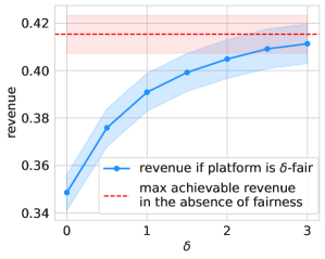
(a) Platform’s revenue.

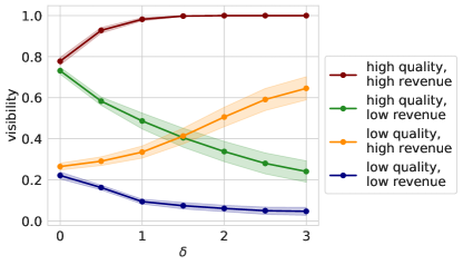
(b) Visibility received by items.

Figure 1: We solve Problem (fair) with $n=4$ and $K=2$, where the four items respectively have high/low qualities and high/low revenues. Here, the platform’s objective is to maximize its revenue, while the items consider visibility as their outcome. The high (low) quality scores $q_{i}$’s are independently drawn from a uniform distribution in $[0.5,1]$ ($[0,0.5]$); the high (low) revenues $r_{i}$’s are independently drawn from a uniform distribution in $[0.6,1]$ ($[0.2,0.6]$). The left plot shows platform’s average revenue ($\pm\textbf{std}/\sqrt{50}$) when it chooses to be $\delta$-fair; the right plot shows how the level of fairness ($\delta$) impacts the mean visibility ($\pm\textbf{std}/\sqrt{50}$) received by each item. All values are averaged over 50 random instances.

To ensure both revenue maximization for the platform and fairness for all items, we adhere to the standard of assortment planning and prioritize revenue maximization as the primary objective, and additionally introduce pairwise constraints to promote fairness among the items. Enforcing fairness through constraints is also seen in works such as Singh and Joachims (2018, 2019) that study fair ranking problems, Cohen et al. (2021a, b) that study fair pricing strategies, Zafar et al. (2019) that studies fair classification, Høgsgaard et al. (2023) that studies the interpolation between fairness and welfare, and Kasy and Abebe (2021) that studies fairness in algorithmic decision-making. That being said, introducing fairness constraints to the assortment planning problem presents new challenges, necessitating close consideration of our problem structure.

4.2 Generality of Our Fairness Notion

Our pairwise fairness notion in Equation (2) is designed to ensure parity of pairwise normalized outcome across different items, and as discussed in Section 3, it is applicable to a variety of metrics of outcome such as visibility, revenue, market share, and more. The use of a generic notion is motivated by the fact that items, depending on their specific contexts, may lay more emphasis on different metrics. For an e-commerce platform, items (i.e., products) may care more about their sales revenue, while for a social media platform, items (i.e., posts) may care more about their visibility or engagement metrics (e.g., likes, comments, shares). Additionally, it is not always clear which notion of fairness should be prioritized from the platform’s perspective, which can be seen from the following example.

In Figure 2, we numerically compare the platform’s expected revenue when it chooses to be fair to its items when the outcome is perceived as either visibility (i.e., $O_{i}(S)=1$ for $i\in S$) or revenue (i.e., $O_{i}(S)=\frac{r_{i}w_{i}}{1+w(S)}$ for $i\in S$), in a number of synthetically generated instances. Here, to illustrate the difference between the two notions of fairness, we solve Problem (fair) exactly when the platform chooses to be $0$-fair with respect to either visibility or expected revenue of items. The comparison in Figure 2 suggests that neither notion of fairness is guaranteed to out-compete the other under all types of settings. Rather, the impact of fairness notions on the platform’s expected revenue depends on a multiplicity of factors, such as price sensitivity and purchasing power of the market, as well as the distribution of popularity weights/revenues of items. Our generic notion allows the platform to tailor the fairness constraint based on their specific needs.

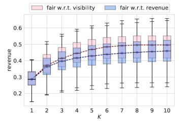
(a) The setting of low price sensitivity $(\beta=-1)$.

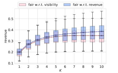
(b) The setting of high price sensitivity $(\beta=-0.1)$.

Figure 2: We solve Problem (fair) with $n=10$ and $1\leq K\leq n$. For each item $i\in[n]$, $r_{i}\overset{i.i.d}{\sim}\textsc{Unif}\left([0,1]\right)$, and $w_{i}=\exp(\beta\cdot r_{i}+\theta_{i})$, where $\beta$ is a price sensitivity parameter. We take $\theta_{i}\overset{i.i.d}{\sim}\textsc{Unif}\left([0.4,1]\right)$ if $i\leq m$ and $\theta_{i}\overset{i.i.d}{\sim}\textsc{Unif}\left([0.2,0.4]\right)$ if $i>m$, where $1\leq m\leq\lceil n/4\rceil$ is the number of highly attractive items. A similar setup of synthetically generated instance is adopted in our numerical studies in Section 16. We set $q_{i}=w_{i}$ for all $i\in[n]$. For each value of $(K,m,\beta)$, we generate $50$ random instances and numerically compute the objective of Problem (fair) when we are $0$-fair under different notions of fairness. Figure 2a shows that in a market with lower price sensitivity, being fair with respect to item’s visibility yields higher platform’s expected revenue, while Figure 2b shows that in a market with higher price sensitivity, being fair with respect to item’s expected revenue is more profitable for the platform.

4.3 Applicability of Our Model and Method: A Short Overview of Our Case Study

We briefly overview the results from our case study on the MovieLens dataset (Section 9) to highlight the applicability of our model and methods. In our case study, we solve a fair assortment planning problem in the movie recommendation context, with visibility being the outcome received by each movie. Our methods are shown to be not only adaptive, allowing the platform to adjust the level of fairness based on their needs, but also tractable, with the approximate algorithms achieving polynomial runtime and fast computational performance.

In Figure 3, we present the resulting visibility received by each movie under varying levels of fairness, when we apply our $1/2$-approx. algorithm to solve Problem (fair) in the movie recommendation setup. Here, movies are ordered according to decreasing quality. The figure indicates that even under fairness constraints, our approach ensures that the top items receive high visibility while the remaining items are not entirely neglected. This highlights the adaptability of our approach, as the platform can adjust the level of fairness by tuning the fairness parameter $\delta$. We invite the readers to consult Section 9 for a detailed account of our case study.

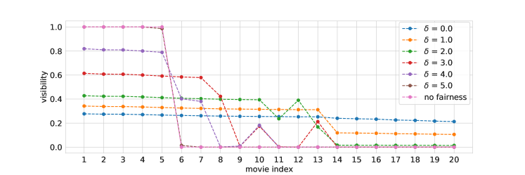
Figure 3: In Section 9, we conduct a case study on the MovieLens dataset. This plot is a preview of the visibility that each movie $i$ receives when we choose to recommend at most $K=5$ movies out of $n=20$ under different levels of fairness $\delta$, when we use our $1/2$-approx. to solve Problem (fair) Here, the indices are decreasing based on movie qualities, and the outcome received by each movie is its visibility.

5 (Near) Optimal Algorithms for Problem (FAIR)

In this section, we start by presenting some main properties of Problem (fair) that motivate the design of our algorithms (Section 5.1). We then present a general framework that allows us to provide a wide-range of (near-)optimal algorithms for Problem (fair), which relies on the dual counterpart of Problem (fair) (Section 5.2) and the Ellipsoid method (Section 5.3).

5.1 Main Properties of Problem (FAIR)

As we discussed earlier, without the fairness constraints, Problem (fair) admits a simple optimal solution under which a single set is offered to users (see Rusmevichientong et al. (2010) for an algorithm that finds the optimal set in polynomial time). Let $S_{K}$ be the set with the maximum expected revenue, i.e., $S_{K}=\mathop{\rm arg\,max}_{|S|\leq K}\textsc{rev}(S)$. Then, without the fairness constraints, the optimal solution to Problem (fair) sets $p(S_{K})=1$ and $p(S)=0$ for any other sets $S\neq S_{K}$. However, such a solution may not be feasible for Problem (fair) in the presence of fairness constraints. To see that, consider item $i\in S_{K}$ and $j\notin S_{K}$. Then, in the aforementioned solution, while item $i$ receives outcome $O_{i}=O_{i}(S_{K})$, item $j$ gets zero outcome (i.e., $O_{j}=0$), violating Constraint (2) (i.e., $\frac{O_{i}}{q_{i}}-\frac{O_{j}}{q_{j}}\leq\delta$) for a sufficiently small $\delta$.

This discussion sheds light on the fact that an optimal solution to Problem (fair) may involve randomization over multiple sets, which might lead to difficulties in practical implementations. However, those concerns can be alleviated, as we show in the following theorem that for any $\delta\geq 0$, there exists an optimal solution to Problem (fair) that involves randomization over at most $\mathcal{O}(n^{2})$ sets, easing implementation of the optimal solution.

Theorem 5.1 (Randomization over at most $\mathcal{O}(n^{2})$ sets)

For any $\delta\geq 0$, there exists an optimal solution $p^{\star}(.)$ to Problem (fair) such that

$$\big{|}\{S:p^{\star}(S)>0\}\big{|}\leq n(n-1)+1.$$

Motivated by Theorem 5.1 above, we aim to design (near-)optimal algorithms for Problem (fair) that also randomize over a polynomial number of sets. We proceed to discuss our framework for finding such solutions in Sections 5.2 and 5.3.

5.2 Dual Counterpart of Problem (FAIR)

Our framework relies on the dual counterpart of Problem (fair), which can be written as

$$\begin{aligned} \textsc{fair-dual}~{}=~{}\min_{\rho\geq 0,\mathbf{z}\geq\mathbf{0}}~{}~{}&\,\rho+\sum_{i=1}^{n}\sum_{j=1,j\neq i}^{n}\delta\cdot q_{i}q_{j}\cdot z_{ij}\\ \text{ s.t. }&\sum_{i\in S}O_{i}(S)\cdot\left(\sum_{j=1,j\neq i}^{n}(z_{ij}-z_{ji}){q}_{j}\right)+\rho\geq\textsc{rev}(S),\quad&\forall S:|S|\leq K\,.\end{aligned}$$ (fair-dual)

Here, $\mathbf{z}=(z_{ij})_{i,j\in[n],i\neq j}$ are the dual variable of the first set of constraints and $\rho\geq 0$ is the dual variable of the second constraint in Problem (fair). Note that $z_{ij}$ can be viewed as the fairness cost that item $i$ has caused due to the presence of item $j$ on the platform. We call each constraint in Problem (fair-dual) a dual fairness constraint on set $S$.

Observe that the set of dual fairness constraints in Problem (fair-dual) can be written as the following single constraint:

$$\rho\geq\max_{S:|S|\leq K}\left\{\textsc{rev}(S)-\sum_{i\in S}O_{i}(S)\cdot\left(\sum_{j=1,j\neq i}^{n}(z_{ij}-z_{ji}){q}_{j}\right)\right\}:=\max_{S:|S|\leq K}~{}\textsc{rev-cost}(S,\mathbf{z})\,.$$ (4)

In the optimal solution of Problem (fair-dual), the inequality in Equation (4) must be satisfied with equality. Here, we refer to $\textsc{rev-cost}(S,\mathbf{z})$ as the cost-adjusted revenue. Recall that $O_{i}(S)=\frac{a_{i}w_{i}}{1+w(S)}+b_{i}$; we can thus reformulate the cost-adjusted revenue as:

$$\textsc{rev-cost}(S,\mathbf{z}) =\textsc{rev}(S)-\sum_{i\in S}\left(\frac{a_{i}w_{i}}{1+w(S)}+b_{i}\right)\cdot c_{i}(\mathbf{z})=\sum_{i\in S}\frac{(r_{i}-a_{i}c_{i}(\mathbf{z}))w_{i}}{1+w(S)}-\sum_{i\in S}b_{i}c_{i}(\mathbf{z})\,,$$ (5)

where for dual vector $\mathbf{z}$, for any $i\in[n]$, we define $c_{i}(\mathbf{z})$ as the cost of item $i$:

$$c_{i}(\mathbf{z})=\sum_{j=1,j\neq i}^{n}(z_{ij}-z_{ji}){q}_{j}\,.$$ (6)

which is a linear combination of the fairness costs $z_{ij}$ and $z_{ji}$, $j\neq i$. Let us additionally define $\mathcal{r}_{i}(\mathbf{z})=r_{i}-a_{i}c_{i}(\mathbf{z})$ as the post-fairness revenue of item $i$ and $\mathfrak{c}_{i}(\mathbf{z})=b_{i}c_{i}(\mathbf{z})$ as the post-fairness cost of item $i$. The cost-adjusted revenue in Equation (5) can then be further simplified as:

$$\textsc{rev-cost}(S,\mathbf{z}) =\sum_{i\in S}\frac{\mathcal{r}_{i}(\mathbf{z})w_{i}}{1+w(S)}-\sum_{i\in S}\mathfrak{c}_{i}(\mathbf{z})\,,$$ (7)

Determining the feasibility of any solution for Problem (fair-dual) boils down to solving the optimization problem in Equation (4). However, the following theorem shows that the maximization of cost-adjusted revenue is in general NP-complete.

Theorem 5.2 (Complexity of Determining Feasibility for Problem (fair-dual))

Consider the following problem that represents the first set of constraints in Problem (fair-dual):

$$\textsc{sub-dual}(\mathbf{z},K)=\max_{S:|S|\leq K}~{}\textsc{rev-cost}(S,\mathbf{z})\,, \mathbf{z},K$$ (sub-dual())

where $\textsc{rev-cost}(S,\mathbf{z})$ is defined in Equation (7).

1. For revenue/marketshare-fair instances where $\Theta=(\textbf{a},0,\textbf{r},\textbf{w},\textbf{q})$, there exists an polynomial-time optimal algorithm for Problem (sub-dual($\mathbf{z},K$)).

2. For visibility-fair and general instances where $\Theta=(\textbf{a},\textbf{b},\textbf{r},\textbf{w},\textbf{q})$, with $b_{i}\neq 0$ for some $i\in[n]$, Problem (sub-dual($\mathbf{z},K$)) is NP-complete. In particular, even for visibility-fair instances with uniform revenues (i.e, $r_{i}=r$ for any $i\in[n]$), Problem (sub-dual($\mathbf{z},K$)) is also NP-complete.

Theorem 5.2 implies the possibility to design a polynomial-time optimal algorithm for Problem (fair) in revenue/marketshare-fair instances. However, for visibility-fair and more general instances (e.g., if the platform wishes to consider a weighted sum of revenue and visibility as the outcome received by an item), verifying the feasibility of solutions in Problem (fair-dual) may be computationally intractable. To address this, we will soon demonstrate in Section 5.3 that with a polynomial-time near-optimal algorithm for Problem (sub-dual($\mathbf{z},K$)), we can use the Ellipsoid method to solve Problem (fair) near-optimally in polynomial time.

5.3 Fair Ellipsoid-based Framework

We now present our framework for obtaining (near-)optimal solutions to Problem (fair), which relies on the Ellipsoid method and the dual problem (fair-dual). We will show that to obtain a $\beta$-approximate solution to Problem (fair), for some $\beta\in(0,1]$, that randomizes over a polynomial number of assortments, it suffices to have a $\beta$-approximate solution to Problem (sub-dual($\mathbf{z},K$)). (Here, when $\beta=1$, a $\beta$-approximate solution is an optimal solution.) See Theorem 5.3 stated at the end of this section. In particular, the (near-)optimal algorithm for Problem (fair-dual) will play the role of an (approximate) separation oracle for the Ellipsoid method (see Padberg (2013)) that we apply to the dual problem (fair-dual).

Assume that we have access to a polynomial-time algorithm $\mathcal{A}$ that gives a $\beta$-approximate solution for (sub-dual($\mathbf{z},K$)), for any $\mathbf{z}\geq 0$ and $K\in[n]$, where $\beta\in(0,1]$. We propose a fair Ellipsoid-based algorithm that consists of the following two steps:

Step 1: Apply the Ellipsoid method to the dual problem (fair-dual) using a $\beta$-approximate separation oracle.

We first apply the Ellipsoid method to solving Problem (fair-dual). Recall that Problem (fair-dual) has exponentially many constraints; further, the first set of constraints in Problem (fair-dual) can be written as $\rho\geq\max_{S:|S|\leq K}~{}\textsc{rev-cost}(S,\mathbf{z})=\textsc{sub-dual}(\mathbf{z},K)$, which is shown to be NP-complete (see Theorem 5.2). As a result, at each iteration of the Ellipsoid method, instead of applying an exact separation oracle, we apply the following approximate separation oracle to check whether the current solution $(\mathbf{z},\rho)$ is feasible, and, if not, finds a violated constraint.

1. We first apply the polynomial-time $\beta$-approximate algorithm $\mathcal{A}$ to Problem (sub-dual($\mathbf{z},K$)), which returns $S_{\mathcal{A}}$ with $|S_{\mathcal{A}}|\leq K$ such that $\textsc{rev-cost}(S_{\mathcal{A}},\mathbf{z})\geq\beta\cdot\textsc{sub-dual}(\mathbf{z},K)$.

2. We then determine whether the current solution $(\mathbf{z},\rho)$ is feasible. If $\textsc{rev-cost}(S_{\mathcal{A}},\mathbf{z})>\rho$, the separation oracle has found the violating constraint: set $S_{\mathcal{A}}$ violates the dual fairness constraint. If $\textsc{rev-cost}(S_{\mathcal{A}},\mathbf{z})\leq\rho$, the separation oracle will declare the solution $(\mathbf{z},\rho)$ feasible.

In Section 12, we formally present the Ellipsoid method for Problem (fair-dual) used in Step 1; see Algorithm 3 for more details.

Step 2: Solve Problem (fair) using only sets for which the dual fairness constraint is violated.

Throughout the run of the Ellipsoid method, we keep track of all the sets that have violated the dual fairness constraint at some iteration. Let $\mathcal{V}\subset\{S:|S|\leq K\}$ be the collection of sets for which the dual fairness constraint has been violated in the Ellipsoid method. We will show, in the proof of Theorem 5.3, that $|\mathcal{V}|$ is polynomial in $n$ and $\log(q_{\max})$. Here, $q_{\max}\in\mathbb{Z}^{+}$ is the maximum adjusted measurement of quality, where, for any rational $q_{i}$, its adjusted version is obtained by multiplying it by the smallest common denominator of all the quality values. We then solve the primal problem (fair) by additionally setting $p(S)=0$ for all $S\notin\mathcal{V}$. This reduces the number of non-zero variables in Problem (fair) to a polynomial size, and allows us to solve it in polynomial time.

In the following theorem, we show that the fair Ellipsoid-based algorithm above (i) gives a $\beta$-approximate solution for Problem (fair), which only randomizes over a polynomial number of assortments, and (ii) runs in polynomial time.

Theorem 5.3 ($\beta$-Approximate Algorithm for Problem (FAIR))

Suppose that for any $\mathbf{z}\geq\mathbf{0}$ and $K\in[n]$, we have a polynomial-time $\beta$-approximate algorithm $\mathcal{A}$ for Problem (sub-dual($\mathbf{z},K$)), for some $\beta\in(0,1]$. That is, $\mathcal{A}$ returns set $S_{\mathcal{A}}$ with $|S_{\mathcal{A}}|\leq K$ such that

$$\textsc{rev-cost}(S_{\mathcal{A}},\mathbf{z})\geq\beta\cdot\textsc{sub-dual}(\mathbf{z},K)\,.$$

Then, there exists a polynomial-time algorithm that returns a $\beta$-approximate feasible solution $\widehat{p}(S)$, $S\subseteq[n]$ to Problem (fair). That is, $\sum_{S:|S|\leq K}\widehat{p}(S)\cdot\textsc{rev}(S)\geq\beta\cdot\ref{eq:problem:fair}$ and the returned solution is $\delta$-fair. In addition, the number of sets $S$ such that $\widehat{p}(S)>0$ is polynomial in $n$ and $\log(q_{\max})$, where $q_{\max}\in\mathbb{Z}^{+}$ is the maximum adjusted measurement of quality.

In light of Theorems 5.2 and 5.3, our goal in the following section is to design a polynomial-time $\beta$-approximate algorithm for Problem (sub-dual($\mathbf{z},K$)). This, together with the fair Ellipsoid-based framework discussed above, will then result in a polynomial-time $\beta$-approximate algorithm for our original Problem (fair), which we call a $\beta$-approximate fair Ellipsoid-based algorithm.

6 (Near) Optimal Algorithms for Problem (sub-dual($\mathbf{z},K$))

In this section, we focus on designing a polynomial-time $\beta$-approximate algorithm for Problem (sub-dual($\mathbf{z},K$)), which we can use as a (near-)optimal separation oracle for Problem (fair-dual) as we apply the Ellipsoid-based algorithm in Section 5.3. Since the dual vector $\mathbf{z}$ is fixed when we solve Problem (sub-dual($\mathbf{z},K$)) at each iteration of the Ellipsoid method, in what follows, we suppress the dependency of variables on $\mathbf{z}$ and denote $\mathcal{r}_{i}=\mathcal{r}_{i}(\mathbf{z})$ and $\mathfrak{c}_{i}=\mathfrak{c}_{i}(\mathbf{z})$.

Recall from Theorem 5.2 that achieving optimality for Problem (sub-dual($\mathbf{z},K$)) is only possible for revenue/marketshare-fair instances, while for visibility-fair and general instances, the problem is NP-complete. Hence, in Section 6.1, we first briefly discuss how one can solve Problem (sub-dual($\mathbf{z},K$)) optimally for revenue/marketshare-fair instances. In Section 6.2, we move on to work with general instances and discuss how to design approximation algorithms for Problem (sub-dual($\mathbf{z},K$)). In particular, we present an important transformation that shows solving Problem (sub-dual($\mathbf{z},K$)) is equivalent to solving an infinite series of knapsack problems with both cardinality and capacity constraints. This novel transformation will prove to be crucial to the design of all our approximation algorithms ($1/2$-approx. algorithm, PTAS, FPTAS) for Problem (sub-dual($\mathbf{z},K$)); see Sections 7, 8, and 15.

6.1 Optimal Algorithm for Revenue/Marketshare-Fair Instances

Recall that in revenue/marketshare-fair instances, we have $b_{i}=0$, and hence $\mathfrak{c}_{i}=0$ for all $i\in[n]$. In this case, Problem (sub-dual($\mathbf{z},K$)) simplifies to a capacitated assortment optimization problem, with $\mathcal{r}_{i}$ being the revenue associated with each item $i$. There exists a polynomial-time algorithm that can solve Problem (sub-dual($\mathbf{z},K$)) optimally.

Proposition 6.1

Given any revenue/marketshare-fair instance with the form $\Theta=(\textbf{a},0,\textbf{r},\textbf{w},\textbf{q})$, the StaticMNL algorithm in Rusmevichientong et al. (2010) returns the optimal assortment $S^{\star}=\mathop{\rm arg\,max}_{S:|S|\leq K}~{}\textsc{rev-cost}(S,\mathbf{z})$, and its running time is of order $\mathcal{O}(n^{2})$.

The StaticMNL algorithm exploits the structural properties associated with the MNL model to return a sequence of $\mathcal{O}(n^{2})$ assortments that is guaranteed to contain the optimal assortment. With the help of the StaticMNL algorithm, we have access to an exact separation oracle for Problem (fair-dual). This, along with the Ellipsoid-based algorithm in Section 5.3, allows us to solve Problem (fair) optimally in polynomial-time.

6.2 Near Optimal Algorithm for General Instances

In visibility-fair and general instances, however, solving Problem (sub-dual($\mathbf{z},K$)) is NP-complete and requires us to design approximation algorithms. We observe that given any instance $\Theta=(\textbf{a},\textbf{b},\textbf{r},\textbf{w},\textbf{q})\in\mathbb{R}_{+}^{5n}$, solving Problem (sub-dual($\mathbf{z},K$)) is equivalent to solving a capacitated assortment optimization problem with fixed costs, where post-fairness revenue $\mathcal{r}_{i}$ serves as the revenue of item $i$ and post-fairness cost $\mathfrak{c}_{i}$ is the fixed cost of item $i$. This problem has been considered as a challenging yet important problem in the retail industry (Caro and Martḿissinginez-de Albéniz 2015, Kunnumkal and Martínez-de Albéniz 2019). However, even without the capacity constraints, assortment optimization with fixed costs has been shown to be a NP-complete problem, and existing works have proposed intricate methods for its approximation (Kunnumkal et al. 2010, Kunnumkal and Martínez-de Albéniz 2019).

In order to design polynomial-time approximation algorithms for Problem (sub-dual($\mathbf{z},K$)), or more generally, for capacitated assortment optimization with fixed costs, we will exploit the structural properties associated with the MNL model with fixed costs in the design of our approximation algorithms. It is important to note that the structure of our problem has become more challenging than the one investigated in Rusmevichientong et al. (2010), due to the existence of fixed costs. To tackle this challenge, we start by first establishing an important equivalence which transforms Problem (sub-dual($\mathbf{z},K$)) to an infinite series of parameterized knapsack problems, with both cardinality and capacity constraints.

Consider the following knapsack problem with capacity $W\geq 0$ and cardinality constraint $K$:

$$\textsc{kp}(W,K)=\max_{S} \sum_{i\in S}\left(\frac{\mathcal{r}_{i}w_{i}}{1+W}-\mathfrak{c}_{i}\right) \textsc{kp}(W,K)$$ ()

s.t. $$\sum_{i\in S}w_{i}\leq W\quad\text{and}\quad|S|\leq K\,.$$

where the utility of item $i\in[n]$ is $\frac{\mathcal{r}_{i}w_{i}}{1+W}-\mathfrak{c}_{i}$ and its weight is $w_{i}$. For a given $W$, we denote the utility of item $i$ as $u_{i}(W):=\frac{\mathcal{r}_{i}w_{i}}{1+W}-\mathfrak{c}_{i}$. Observe that in Problem ($\textsc{kp}(W,K)$), the first constraint is the capacity constraint and the second constraint is the cardinality constraint. The former ensures that the sum of the weight of the items that are added to the knapsack does not exceed $W$ and the latter ensures that at most $K$ items are added to the knapsack.

The following theorem characterizes the relationship between Problems ($\textsc{kp}(W,K)$), $W\geq 0$, and Problem (sub-dual($\mathbf{z},K$)).

Theorem 6.2 (Problem (SUB-DUAL$(\mathbf{z},K)$) as an infinite series of knapsack problems)

For any $\mathbf{z}\geq\mathbf{0}$ and $K\in[n]$, we have

$$\textsc{sub-dual}(\mathbf{z},K)=\max_{W\geq 0}~{}\textsc{kp}(W,K)\,.$$

In light of Theorem 6.2, to design a $\beta$-approximate algorithm for Problem (sub-dual($\mathbf{z},K$)), we can instead design a $\beta$-approximate algorithm for $\max_{W\geq 0}\textsc{kp}(W,K)$, which finds a set $S$ such that $\textsc{rev-cost}(S,\mathbf{z})\geq\beta\cdot\max_{W\geq 0}\textsc{kp}(W,K)$. Observe that the problem $\max_{W\geq 0}~{}\textsc{kp}(W,K)$ requires us to solve an infinite number of cardinality-constrained knapsack problems, i.e., $\textsc{kp}(W,K)$, for any $W\geq 0$. Further note that in the cardinality-constrained knapsack problem $\textsc{kp}(W,K)$, as we increase $W$, the capacity of the knapsack enlarges, but the utility of the items decreases. (Recall that the utility of item $i$ is $u_{i}(W)=\frac{\mathcal{r}_{i}w_{i}}{1+W}-\mathfrak{c}_{i}$). Hence, it is unclear which value of $W$ maximizes $\textsc{kp}(W,K)$ and more importantly, if our transformation has simplified the problem.

As we will show in the following sections, this transformation in conjunction with taking advantage of the structure of cardinality-constrained knapsack problems $\textsc{kp}(W,K)$ as a function of $W$ leads to a number of near-optimal algorithms for Problem (sub-dual($\mathbf{z},K$)). In Section 7, we start by presenting a $1/2$-approx. algorithm for Problem (sub-dual($\mathbf{z},K$)). Then, with the help of our $1/2$-approx. algorithm, we further present a PTAS for Problem (sub-dual($\mathbf{z},K$)) in Section 8, which obtains a $(1-\epsilon)$-approximate solution for any $\epsilon>0$, in time polynomial in $n$ and $K$. We also show in Section 15 that an even stronger theoretical guarantee (an FPTAS) is achievable in the special case when we work with a visibility-fair instance with uniform revenues (i.e., $r_{i}=r$ for all $i\in[n]$), which is of special interest to platforms that seek to maximize their market share or those that adopt a fixed commission model.

7 1/2-Approx. Algorithm for Problem (sub-dual($\mathbf{z},K$))

We first present a $1/2$-approx. algorithm for general instances of Problem (sub-dual($\mathbf{z},K$)), by using the key transformation to an infinite series of knapsack problems $\max_{W\geq 0}\textsc{kp}(W,K)$. Combining this with the fair Ellipsoid-based framework in Section 5.3, we obtain a $1/2$-approx. fair ellipsoid-based algorithm for general instances of our problem.

In Section 7.1, we start by discussing the LP relaxation of our knapsack problems and introducing an important notion of profile, which is the key to the design of our $1/2$-approx. algorithm. In Section 7.2, we present our $1/2$-approx. algorithm for $\max_{W\geq 0}\textsc{kp}(W,K)$ and describe our main intuitions behind each step. In Section 7.3, we formally characterize the approximation ratio and time complexity of our $1/2$-approx. algorithm.

7.1 Relaxed Knapsack Problems and the Notion of Profile

To design a $1/2$-approx. algorithm for this infinite series of knapsack problems, we take advantage of the LP relaxation of the original knapsack problem ($\textsc{kp}(W,K)$), defined as

$$\textsc{kp-relax}(W,K)=\max_{\mathbf{x}\in[0,1]^{n}} \sum_{i\in[n]}(\frac{\mathcal{r}_{i}w_{i}}{1+W}-\mathfrak{c}_{i})x_{i} \textsc{kp-relax}(W,K)$$ ()

$$\mathrm{s.t.} \sum_{i\in[n]}w_{i}x_{i}\leq W\quad{\text{and}}\quad\sum_{i\in[n]}{x_{i}}\leq K\,.$$

Observe that if we enforce $x_{i}\in\{0,1\}$, rather than $x_{i}\in[0,1]$, we recover Problem ($\textsc{kp}(W,K)$). The variable $x_{i}$, $i\in[n]$, can be viewed as the fraction of item $i$ that we fit in the knapsack. For integer solutions $\mathbf{x}\in\{0,1\}^{n}$ to Problem ($\textsc{kp-relax}(W,K)$), we sometimes use the term “sets” where the set associated with $\mathbf{x}\in\{0,1\}^{n}$ is $\{i\in[n]:x_{i}=1\}$.

For any fixed $W\in[0,\infty)$, the relaxed problem ($\textsc{kp-relax}(W,K)$) always admits an optimal basic (feasible) solution. Further, any optimal basic solution to Problem ($\textsc{kp-relax}(W,K)$) has at most two fractional variables (see Lemma 1 in Caprara et al. (2000)). Let $\mathbf{x}^{\star}(W)$ be an optimal basic solution to Problem ($\textsc{kp-relax}(W,K)$) that has at most two fractional variables. We then define $P_{1}(W)=\{i\in[n]:x^{\star}_{i}(W)=1\}$ as the set of items that have a value of $1$ in $\mathbf{x}^{\star}(W)$, which are the items fully added to the knapsack associated with Problem ($\textsc{kp-relax}(W,K)$). Similarly, we define $P_{f}(W)=\{i\in[n]:0<x^{\star}_{i}(W)<1\}$ (respectively $P_{0}(W)=\{i\in[n]:x^{\star}_{i}(W)=0\}$) as the set of items that have a fractional value (respectively value of zero) in $\mathbf{x}^{\star}(W)$. (Here, “f” in $P_{f}$ stands for fractional.) As stated earlier, $|P_{f}(W))|\leq 2$ and hence, here we denote $P_{f}(W)$ by an ordered pair of items $(\textsf{i},\textsf{j})$. When the fractional set $P_{f}(W)$ is empty, both $\textsf{i},\textsf{j}$ would be a dummy item and, in particular, the no-purchase item $0$. When the fractional set $P_{f}(W)$ has a single item, we set $\textsf{j}=0$. Finally, when the fractional set $P_{f}(W)$ has two items, we have $w_{\textsf{i}}\leq w_{\textsf{j}}$. For any set $S$, we let $S\cup\{0\}=S$ and $S\setminus\{0\}=S$; that is, the addition or removal of a dummy item does not affect the set itself. We refer to sets $\mathcal{P}(W)=\{P_{1}(W),P_{f}(W),P_{0}(W)\}$ as the profile associated with the optimal basic solution $x^{\star}(W)$.

In the following lemma, borrowed from Caprara et al. (2000), we show that using an optimal basic solution to the relaxed knapsack problem ($\textsc{kp-relax}(W,K)$), we can construct an integer $1/2$-approx. solution to Problem ($\textsc{kp-relax}(W,K)$), which also serves as an $1/2$-approx. solution to Problem ($\textsc{kp}(W,K)$).

Lemma 7.1 ($1/2$-Approx. Solutions to Problem ($\textsc{kp-relax}(W,K)$) (Caprara et al. 2000))

For a fixed $W\in[0,\infty)$, let $\mathbf{x}^{\star}(W)$ be an optimal basic solution to Problem ($\textsc{kp-relax}(W,K)$) and let $\mathcal{P}(W)=\left\{P_{1}(W),P_{f}(W),P_{0}(W)\right\}$ be its associated profile, where $P_{f}(W)=(\textsf{i},\textsf{j})$. We have one of the following:

1. No fractional variable. If $P_{f}(W)=(0,0)$, $P_{1}(W)$ is an integer optimal solution to Problem ($\textsc{kp-relax}(W,K)$).

2. One fractional variable. If $P_{f}(W)=(\textsf{i},0)$ for some $\textsf{i}\in[n]$, either $P_{1}(W)$ or $\{\textsf{i}\}$ is an integer $1/2$-approx. solution to Problem ($\textsc{kp-relax}(W,K)$).

3. Two fractional variables. If $P_{f}(W)=(\textsf{i},\textsf{j})$ for some $\textsf{i},\textsf{j}\in[n]$ such that $w_{\textsf{i}}\leq w_{\textsf{j}}$, either $P_{1}(W)\cup\{\textsf{i}\}$ or $\{\textsf{j}\}$ is an integer $1/2$-approx. solution to Problem ($\textsc{kp-relax}(W,K)$).

It is clear from Lemma 7.1 that for any given $W\in[0,\infty)$, as long as we know the profile of the optimal basic solution to the relaxed problem ($\textsc{kp-relax}(W,K)$), we can find a $1/2$-approx. solution for Problem ($\textsc{kp}(W,K)$). However, in our problem, i.e., $\max_{W\geq 0}~{}\textsc{kp}(W,K)$, we need to find approximate solutions for an infinite number of knapsack problems, defined on the interval $W\in[0,\infty)$. While solving one relaxed knapsack problem is doable in polynomial time, we cannot possibly solve an infinite number of them in order to find the corresponding approximate solutions.

The key observation that we make here is that to find a $1/2$-approx. solution of Problem ($\textsc{kp}(W,K)$) or ($\textsc{kp-relax}(W,K)$), the only information that we need is the profile $\mathcal{P}(W)$, instead of the actual optimal basic solution $\mathbf{x}^{\star}(W)$ to Problem ($\textsc{kp-relax}(W,K)$). While $\mathbf{x}^{\star}(W)$ might keep changing for different knapsack capacities $W$, as we will show later in the proof of Theorem 7.3, their associated profile $\mathcal{P}(W)$ undergoes a polynomial number of changes as $W$ changes. This allows us to consider a polynomial number of sub-intervals where in each sub-interval, the profile $\mathcal{P}(W)$ does not change, and we can consider the same collection of sets to construct a $1/2$-approx. solution. Motivated by the idea outlined above, we propose a $1/2$-approx. algorithm for $\max_{W\geq 0}~{}\textsc{kp}(W,K)$ in which we adaptively partition the interval of $[0,\infty)$ to polynomial number of sub-intervals.

7.2 Description of the 1/2-Approx. Algorithm

We now describe the main procedures of our $1/2$-approx. algorithm for $\max_{W\geq 0}~{}\textsc{kp}(W,K)$, presented in Algorithm 1. As alluded above, a main challenge associated with this problem is that the key components of our knapsack problem (e.g., utilities and capacity constraint) keep evolving as $W$ changes. Our first step in tackling this issue is to partition the interval $[0,\infty)$ into $\mathcal{O}(n^{3})$ sub-intervals, such that each sub-interval $I\subset[0,\infty)$ is well-behaving, which is defined as follows:

Definition 7.2 (Well-behaving interval)

Given a collection of $n$ items, indexed by $i\in[n]$, we say that an interval $I\subset[0,\infty)$ is well-behaving if the following conditions are satisfied on $I$:

1. The signs of the utilities of items are the same for any $W\in I$.

2. The ordering of the utilities of items is the same for $W\in I$.

3. The ordering of the utility-to-weight ratios of items is the same for any $W\in I$. Here, the utility-to-weight ratio of item $i\in[n]$ is $\frac{u_{i}(W)}{w_{i}}=\frac{\frac{\mathcal{r}_{i}w_{i}}{1+W}-\mathfrak{c}_{i}}{w_{i}}=\frac{\mathcal{r}_{i}}{1+W}-\frac{\mathfrak{c}_{i}}{w_{i}}$.

4. For any given item $i\in[n]$ and two distinct items $j\neq i,k\neq i,k\neq j$, the ordering between $\frac{u_{j}(W)-u_{i}(W)}{w_{j}-w_{i}}$ and $\frac{u_{k}(W)-u_{i}(W)}{w_{k}-w_{i}}$ is the same for any $W\in I$.

We start by pre-partitioning the interval $[0,\infty)$ into a number of sub-intervals $I$, such that each of them is the largest well-behaving sub-interval we can obtain. To find such $I$’s, we simply need to find the values of $W$ at which the aforementioned conditions cease to hold. Regarding condition (i), the sign of the utilities of item $i\in[n]$ only changes when $u_{i}(W)=\frac{\mathcal{r}_{i}w_{i}}{1+W}-\mathfrak{c}_{i}=0$, and there are $\mathcal{O}(n)$ such values of $W$. Regarding condition (ii), note that the ordering of utility only changes at the values of $W$ such that $\frac{\mathcal{r}_{i}w_{i}}{1+W}-\mathfrak{c}_{i}=\frac{\mathcal{r}_{j}w_{j}}{1+W}-\mathfrak{c}_{j}$ for some $i\neq j$, and hence there are $\mathcal{O}(n^{2})$ such values of $W$ where the ordering changes. Regarding condition (iii), the utility-to-weight ratio only changes at the values of $W$ such that $\frac{\mathcal{r}_{i}}{1+W}-\frac{\mathfrak{c}_{i}}{w_{i}}=\frac{\mathcal{r}_{j}}{1+W}-\frac{\mathfrak{c}_{j}}{w_{j}}$ for some $i\neq j$, and there are again $\mathcal{O}(n^{2})$ such values of $W$ where the ordering changes. Finally, regarding condition (iv), this condition essentially implies that if we want to replace item $i$ in our knapsack with another item that is not in the knapsack, the ordering of the marginal increase in utility does not change. Note that such ordering only changes at the values of $W$ such that $\frac{u_{j}(W)-u_{i}(W)}{w_{j}-w_{i}}=\frac{u_{k}(W)-u_{i}(W)}{w_{k}-w_{i}}\,,$ and there are $\mathcal{O}(n^{3})$ such values of $W$ where this ordering can change. Overall, there are $\mathcal{O}(n^{3})$ values of $W$ at which the aforementioned conditions experience changes. Hence, we can pre-partition $[0,\infty)$ into $\mathcal{O}(n^{3})$ sub-intervals such that each sub-interval $I$ is the largest sub-interval that is well-behaving.

We now focus our attention on each well-behaving interval $I=[W_{\min},W_{\max})\subset[0,\infty)$ that satisfies the conditions in Definition 7.2. The conditions above essentially guarantee that the key components of the knapsack problems do not change too drastically on any well-behaving interval, which then allows us to perform an adaptive partitioning procedure on $I$. In Algorithm 1, we present a $1/2$-approx. algorithm for $\max_{W\in I}\textsc{kp}(W,K)$. In particular, it returns an integer $1/2$-approx. solution $S_{I}$ for $\max_{W\in I}~{}\textsc{kp-relax}(W,K)$, which also serves as an $1/2$-approx. solution to the problem $\max_{W\in I}\textsc{kp}(W,K)$. Moreover, the algorithm also returns a collection of sets, denoted by $\mathcal{C}_{I}$, such that it always contains a $1/2$-approx. solution to Problem ($\textsc{kp}(W,K)$) for each $W\in I$.

Algorithm 1 $\mathcal{A}_{1/2}(\mathbf{w},\mathbf{\mathcal{r}},\mathbf{\mathfrak{c}},K,I)$:  $1/2$-approx. algorithm for $\max_{W\in I}~{}\textsc{kp}(W,K)$

Input: weights $\mathbf{w}=\{w_{i}\}_{i\in[n]}$, post-fairness revenues $\mathbf{\mathcal{r}}=\{\mathcal{r}_{i}\}_{i\in[n]}$, post-fairness costs $\mathbf{\mathfrak{c}}=\{\mathfrak{c}_{i}\}_{i\in[n]}$, cardinality upper bound $K$, a well-behaving interval $I=[W_{\min},W_{\max})\subset[0,\infty)$ per Definition 7.2.
Output: collection $\mathcal{C}_{I}$ and assortment $S_{I}$.

1. Initialization.

   1. Rank the items by their utility-to-weight ratios. Let $h_{j}$ be the index of the item with the $j$th highest utility-to-weight ratio, for $j\in[n]$, and define $H_{j}=\{h_{1},\dots,h_{j}\}$, for $j\in[K]$ and $W_{\textsc{TH}}=w(H_{K})$.

   2. Initialize the collection of assortments $\mathcal{C}_{I}=\emptyset$. For $j\in[n]$, add $\{j\}$ to $\mathcal{C}_{I}$.

2. Interval $I_{\text{low}}=I\cap[0,W_{\textsc{TH}})$. If $I_{\text{low}}$ is non-empty:

   1. For $j=1,\dots,K$, add $H_{j}$ to $\mathcal{C}_{I}$.

   2. Stopping rule. If $u_{h_{K}}(W_{\textsc{TH}})\geq 0$, go to Step 3; otherwise, go to Step 4 (i.e., the termination step).

3. Interval $I_{\text{high}}=I\cap[W_{\textsc{TH}},\infty)$. If $I_{\text{high}}$ is non-empty:

   1. Initialize the profile.

      • If $W_{\min}<W_{\textsc{TH}}$, set $P_{1}=H_{K},P_{0}=[n]\setminus H_{K}$, and $W_{\text{next}}=W_{\textsc{TH}}$.

      • If $W_{\min}\geq W_{\textsc{TH}}$, compute an optimal basic solution for Problem $(\textsc{kp-relax}(W_{\min},K))$ with profile $\mathcal{P}(W_{\min})=\{P_{1}(W_{\min}),(\textsf{i},\textsf{j}),P_{0}(W_{\min})\}$, where $w_{i}<w_{j}$. Add $P_{1}(W_{\min})\cup\{\textsf{i}\}$ and $P_{1}(W_{\min})\cup\{\textsf{j}\}$ to $\mathcal{C}_{I}$. Set $P_{1}=P_{1}(W_{\min})\cup\{\textsf{j}\}$, $P_{0}=[n]\setminus P_{1}$, and $W_{\text{next}}=w(P_{1})$.

   2. Adaptively partitioning $I_{\text{high}}$. While there exist $i\in P_{1},j\in P_{0}$ such that $w_{i}<w_{j}$:

      1. Update indices $\textsf{i}^{\star},\textsf{j}^{\star}$ as follows:

         $$(\textsf{i}^{\star},\textsf{j}^{\star})\leftarrow\mathop{\rm arg\,max}_{i\in P_{1},j\in P_{0}\atop{w_{i}<w_{j}}}\left[\frac{u_{j}(W_{\text{next}})-u_{i}(W_{\text{next}})}{w_{j}-w_{i}}\right]\,.$$

      2. Stopping rule. If $W_{\text{next}}\geq W_{\text{max}}$ or $u_{\textsf{i}^{\star}}(W_{\text{next}})>u_{\textsf{j}^{\star}}(W_{\text{next}})\,,$ go to Step 4 (i.e., the termination step).

      3. Swapping the two items. Update $P_{1},P_{0},W_{\text{next}}$ as follows:

         $$P_{1}\leftarrow P_{1}\cup\{\textsf{j}^{\star}\}\setminus\{\textsf{i}^{\star}\}\quad\text{and}\quad P_{0}\leftarrow P_{0}\cup\{\textsf{i}^{\star}\}\setminus\{\textsf{j}^{\star}\}\quad\text{and}\quad W_{\text{next}}\leftarrow W_{\text{next}}-w_{\textsf{i}^{\star}}+w_{\textsf{j}^{\star}}\,.$$

         Add $P_{1}$ to $\mathcal{C}_{I}$.

4. Termination Step. Return the collection $\mathcal{C}_{I}$ and set $S_{I}=\mathop{\rm arg\,max}_{S\in\mathcal{C}_{I}}\textsc{rev-cost}(S,\mathbf{z})$.

We define $H_{j}=\{h_{1},\dots,h_{j}\}\subset[n]$ as the $j$ items in $[n]$ with the highest utility-to-weight ratios. Recall that on a well-behaving interval $I$, the ordering of utility-to-weight ratios of items does not change, so the sets $\{H_{j}\}_{j=1}^{K}$ are well-defined. In Algorithm 1, we partition $I=[W_{\min},W_{\max})$ into two intervals $I_{\text{low}}=I\cap[0,W_{\textsc{TH}})$ and $I_{\text{high}}=I\cap[W_{\textsc{TH}},\infty)$, where $W_{\textsc{TH}}=w(H_{K})$ is the total weight of the $K$ items with the highest utility-to-weight ratios. We now discuss $I_{\text{low}}$ and $I_{\text{high}}$ separately.

Interval $I_{\text{low}}=I\cap[0,W_{\textsc{TH}})$. For any $W\in I_{\text{low}}=I\cap[0,W_{\textsc{TH}})$, solving the relaxed problem ($\textsc{kp-relax}(W,K)$) is rather straightforward because or any $W\in I_{\text{low}}$, the cardinality constraint is not binding (recall that $W_{\textsc{TH}}=w(H_{K})$), and hence the solution is simply filling up the knapsack with the items with the highest utility-to-weight ratios until we reach the capacity $W$, regardless of the value of $W$. Therefore, the profile of the optimal basic solution to the relaxed problem, i.e., $\mathcal{P}(W)=\{P_{1}(W),P_{f}(W),P_{0}(W)\}$, always has the following structure:

$$P_{1}(W)=H_{j-1}\,\text{ and }\,P_{f}(W)=(h_{j},0)\quad\text{ for some $j\in[K]$}\,.$$

That explains why in Step 2 of the algorithm, we add sets $H_{j}$, $j=1,\dots,K$, to the collection $\mathcal{C}_{I}$.

Interval $I_{\text{high}}=I\cap[W_{\textsc{TH}},\infty)$. Before discussing how this interval can be handled, we make a few remarks about our stopping rules in Algorithm 1. One crucial observation is that the maximizer of the optimization problem $\mathop{\rm arg\,max}_{W\in I}\textsc{kp-relax}(W,K)$ must be at some value of $W$ for which the capacity constraint of the relaxed problem ($\textsc{kp-relax}(W,K)$) is binding. Our stopping rules in Algorithm 1 essentially checks whether the capacity constraint has become non-binding. First, if $u_{h_{K}}(W_{\textsc{TH}})\leq 0$, where $h_{K}$ is the item with the $K$-th highest utility-to-weight ratio, it is clear that at $W_{\textsc{TH}}$, there are less than $K$ items with positive utilities. In this case, the capacity constraint has become non-binding at $W_{\textsc{TH}}$ and we do not need to examine interval $I_{\text{high}}$ at all; see the stopping rule in Step 2b of Algorithm 1. Second, our algorithm does not necessarily investigate all $W\in I_{\text{high}}$; see the stopping rule in Step 3(b)ii of Algorithm 1. In this step, the algorithm checks if at the current value of $W$, the capacity constraint of $(\textsc{kp-relax}(W,K))$ has become non-binding. If so, increasing $W$ further would no longer be helpful.

We are now ready to discuss interval $I_{\text{high}}$. For $W\in I_{\text{high}}=I\cap[W_{\textsc{TH}},\infty)$, solving the relaxed problem ($\textsc{kp-relax}(W,K)$) becomes more difficult because the profile of the optimal basic solution to the relaxed problem no longer has the nice, pre-specified structure that it had on interval $I_{\text{low}}$. Intuitively, for a large capacity $W$, the cardinally constraint gets binding. With a binding cardinally constraint, it is no longer optimal to fill the knapsack associated with Problem ($\textsc{kp-relax}(W,K)$) with items with the highest utility-to-weight ratios. To handle interval $I_{\text{high}}$, we partition $I_{\text{high}}$ into a polynomial number of sub-intervals, such that on each sub-interval, the profile $\mathcal{P}(W)$ does not change, and hence by Lemma 7.1, we can consider the same approximate solution(s) for this sub-interval. However, the main difficulty here is that these sub-intervals are not known in advance, and hence we have to determine these sub-intervals in an adaptive manner.

Determine sub-intervals adaptively. To determine sub-intervals adaptively, the algorithm keeps updating two quantities as it increases the capacity $W$: (i) capacity change points, denoted by $W_{\text{next}}$, and (ii) two sets that represent the profile at $W_{\text{next}}$. The first set, denoted by $P_{1}$, is $P_{1}(W_{\text{next}})$ that contains all the items that are completely added to the knapsack in Problem $(\textsc{kp-relax}(W_{\text{next}},K))$, and the second set, denoted by $P_{0}$, is $P_{0}(W_{\text{next}})$ that contains all the items that are not added to the knapsack in Problem $(\textsc{kp-relax}(W_{\text{next}},K))$. Note that $W_{\text{next}}$ is chosen such that $P_{f}(W_{\text{next}})$ is empty; that is, $P_{f}(W_{\text{next}})=(0,0)$. To update the sets $P_{1}$ and $P_{0}$, as well as, $W_{\text{next}}$, the algorithm finds two items $\textsf{i}^{\star}\in P_{1}$ and $\textsf{j}^{\star}\in P_{0}$ by solving a simple optimization problem stated in Step 3(b)i. The algorithm then swap these two items—i.e., it removes $\textsf{i}^{\star}$ from $P_{1}$ and adds it to $P_{0}$; and similarly, removes $\textsf{j}^{\star}$ from $P_{0}$ and adds it to $P_{1}$. This is, in fact, one of the main novel aspects of the algorithm that makes obtaining a $1/2$-approx. solution in polynomial time possible.

We now provide more details about the aforementioned swapping idea. Let $W_{\text{next}}$ and $\widehat{W}_{\text{next}}$ be two consecutive capacity change points. Further, let $\textsf{i}^{\star}\in P_{1}(W_{\text{next}})=P_{1}$ and $\textsf{j}^{\star}\in P_{0}(W_{\text{next}})=P_{0}$ with $w_{\textsf{i}^{\star}}<w_{\textsf{j}^{\star}}$ be the solution to optimization problem in Step 3(b)i. That is, $(\textsf{i}^{\star},\textsf{j}^{\star})\in\mathop{\rm arg\,max}_{i\in P_{1},j\in P_{0}\atop{w_{i}<w_{j}}}{(u_{j}(W_{\text{next}})-u_{i}(W_{\text{next}}))}/{(w_{j}-w_{i})}$. At a high level, by solving this optimization problem, we find two items $\textsf{i}^{\star},\textsf{j}^{\star}$ such that swapping them yields the highest marginal increase in utility. Then, after swapping, $\widehat{W}_{\text{next}}=W_{\text{next}}-w_{\textsf{i}^{\star}}+w_{\textsf{j}^{\star}}$ becomes the new capacity change point. For any $W\in(W_{\text{next}},\widehat{W}_{\text{next}})$, both items $\textsf{i}^{\star}$ and $\textsf{j}^{\star}$ are fractional items in the optimal basic solution for Problem ($\textsc{kp-relax}(W,K)$); that is, $P_{f}(W)=(\textsf{i}^{\star},\textsf{j}^{\star})$. As $W$ increases from $W_{\text{next}}$ to $\widehat{W}_{\text{next}}$, the fraction of $\textsf{i}^{\star}$ (i.e., $x^{\star}_{\textsf{i}^{\star}}(W)$) decreases while the fraction of $\textsf{j}^{\star}$ (i.e., $x^{\star}_{\textsf{j}^{\star}}(W)$) increases; See Figure 4. This trend continues until $x^{\star}_{\textsf{i}^{\star}}(W)$ hits zero and $x^{\star}_{\textsf{j}^{\star}}(W)$ hits one, which happens at $W=\widehat{W}_{\text{next}}=W_{\text{next}}-w_{\textsf{i}^{\star}}+w_{\textsf{j}^{\star}}>W_{\text{next}}$. (Note that for all $W\in[W_{\text{next}},\widehat{W}_{\text{next}}]$, we have $x^{\star}_{\textsf{i}^{\star}}(W)+x^{\star}_{\textsf{j}^{\star}}(W)=1$; see Lemma 21.4.) This then leads to $P_{1}(\widehat{W}_{\text{next}})=P_{1}(W_{\text{next}})\cup\{\textsf{j}^{\star}\}\backslash\{\textsf{i}^{\star}\}$ and $P_{0}(\widehat{W}_{\text{next}})=P_{0}(W_{\text{next}})\cup\{\textsf{i}^{\star}\}\backslash\{\textsf{j}^{\star}\}$, which is our swapping idea in Step 3(b)iii. For any other item $i\notin\{\textsf{i}^{\star},\textsf{j}^{\star}\}$, $x_{i}^{\star}(W)$ does not change, and hence the profile stays the same for any $W\in(W_{\text{next}},\widehat{W}_{\text{next}})$, which is $\mathcal{P}(W)=\{P_{1}\setminus\{\textsf{i}^{\star}\},(\textsf{i}^{\star},\textsf{j}^{\star}),P_{0}\setminus\{\textsf{j}^{\star}\}\}$. By Lemma 7.1, this allows us to consider the same candidate set(s) for the interval $[W_{\text{next}},\widehat{W}_{\text{next}})$.

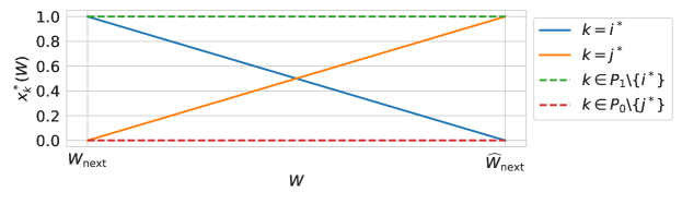
Figure 4: An illustration of how the optimal basic solution $\mathbf{x}^{\star}(W)$ to Problem (KP-RELAX$(W,K)$) changes as $W$ increases from $W_{\text{next}}$ to $\widehat{W}_{\text{next}}$, where $W_{\text{next}},\widehat{W}_{\text{next}}$ are two consecutive change points in $I_{\text{high}}$. Note that $x_{\textsf{i}^{\star}}(W)$ decreases until it hits zero at $\widehat{W}_{\text{next}}$, while $x_{\textsf{j}^{\star}}(W)$ increases until it hits one at $\widehat{W}_{\text{next}}$.

7.3 Performance of Algorithm 1

In the following theorem, we state the main result of Section 7, which shows that Algorithm 1 is a polynomial-time $1/2$-approx. algorithm for Problem (sub-dual($\mathbf{z},K$)).

Theorem 7.3 ($1/2$-Approx. Algorithm)

Consider any interval $I\subset[0,\infty)$ that is well-behaving per Definition 7.2. For any $\mathbf{z}\geq\mathbf{0}$, if we apply Algorithm 1 to interval $I$, and it returns collection $\mathcal{C}_{I}$ and set $S_{I}$, we have that for any $W\in I$, there exists a set $S\in\mathcal{C}_{I}$ such that

$$\textsc{rev-cost}(S,\mathbf{z})\geq\frac{1}{2}~{}\textsc{kp}(W,K)\,.$$

In particular, the set $S_{I}$ satisfies

$$\textsc{rev-cost}(S_{I},\mathbf{z})\geq\frac{1}{2}\max_{W\in I}~{}\textsc{kp}(W,K)\,.$$

Given Algorithm 1, the overall complexity to find a $1/2$-approx. solution for $\max_{W\in I}\textsc{kp}(W,K)$ is in the order of $\mathcal{O}(n^{2}\log n+nK^{2})$.

Recall that to solve $\max_{W\geq 0}\textsc{kp}(W,K)$, we first divide $[0,\infty)$ into $\mathcal{O}(n^{3})$ well-behaving sub-intervals, and then apply Algorithm 1 to each sub-interval. Let $\mathcal{I}$ denote the collection of these sub-intervals. Among the near-optimal assortments we obtained for each sub-interval, we select the one with the highest cost-adjusted revenue, i.e., $S_{1/2}=\mathop{\rm arg\,max}_{S^{\prime}\in\{S_{I}:I\in\mathcal{I}\}}\textsc{rev-cost}(S^{\prime},\mathbf{z})$. This assortment $S_{1/2}$ satisfies $\textsc{rev-cost}(S_{1/2},\mathbf{z})\geq\frac{1}{2}\max_{W\geq 0}\textsc{kp}(W,K)$, which makes it a $1/2$-approx. solution for Problem (sub-dual($\mathbf{z},K$)). The overall complexity for solving Problem (sub-dual($\mathbf{z},K$)) would then be $\mathcal{O}(n^{5}\log n+n^{4}K^{2})$.

Finally, we make a brief remark on a special case where the runtime of the $1/2$-approx. algorithm can be further improved. In a visibility-fair instance where all items generate uniform revenues (recall that this is relevant to platforms that aim to maximize their market share or use a fixed commission model), the $1/2$-approx. algorithm for $\max_{W\geq 0}\textsc{kp}(W,K)$ can be slightly modified and enjoy improved time complexity of $\mathcal{O}(n^{2}\log n+nK^{2})$. See Section 14.1 for more details.

8 PTAS for Problem (sub-dual($\mathbf{z},K$))

In this section, we further propose a PTAS for general instances of Problem (sub-dual($\mathbf{z},K$)), where we again transform the problem to an infinite series of knapsack problems $\max_{W\geq 0}\textsc{kp}(W,K)$. Further, the design of our PTAS crucially relies on the $1/2$-approx. algorithm from Section 7. Combining the PTAS for Problem (sub-dual($\mathbf{z},K$)) with the fair Ellipsoid-based framework in Section 5.3, we obtain a PTAS fair ellipsoid-based algorithm.

Similar to what we did in the design of the $1/2$-approx. algorithm for Problem (sub-dual($\mathbf{z},K$)), we start by pre-partitioning the interval $[0,\infty)$ into at most $\mathcal{O}(n^{3})$ sub-intervals, such that each sub-interval $I$ is well-behaving (see Definition 7.2). Next, we focus on each well-behaving sub-interval $I$ and design a PTAS for $\max_{W\in I}~{}\textsc{kp}(W,K)$. Our PTAS, outlined in Algorithm 2, returns an assortment $S_{I}$ with $|S_{I}|\leq K$ such that $\textsc{rev-cost}(S_{I})\geq(1-\epsilon)\max_{W\in I}~{}\textsc{kp}(W,K)$. In Algorithm 2, we maintain a collection of sets $\mathcal{C}_{I}$ that contains all the sets that could be an integer $(1-\epsilon)$-approx. solution to the problem $\max_{W\in I}\textsc{kp}(W,K)$. We then simply choose the assortment $S_{I}\in\mathcal{C}_{I}$ that gives the highest cost-adjusted revenue.

Algorithm 2 $\text{PTAS}(\mathbf{w},\mathbf{\mathcal{r}},\mathbf{\mathfrak{c}},K,I)$:  PTAS for $\max_{W\in I}~{}\textsc{kp}(W,K)$

Input: weights $\mathbf{w}=\{w_{i}\}_{i\in[n]}$, post-fairness revenues $\mathbf{\mathcal{r}}=\{\mathcal{r}_{i}\}_{i\in[n]}$, post-fairness costs $\mathbf{\mathfrak{c}}=\{\mathfrak{c}_{i}\}_{i\in[n]}$, cardinality upper bound $K$, a well-behaving interval $I=[W_{\min},W_{\max})\subset[0,\infty)$ per Definition 7.2, accuracy parameter $\epsilon\in(0,1)$, and the $1/2$-approx. algorithm $\tilde{\mathcal{A}}_{1/2}$ (Algorithm 6).
Output: assortment $S_{I}$.

1. Initialization. Let $\ell=\min\{\lceil{\frac{1}{\epsilon}-2}\rceil,K\}$. Initialize the collection of assortments $\mathcal{C}_{I}=\emptyset$.

2. Small-sized sets. For each $L\subset[n]$ such that $|L|\leq\ell-1$ and $w(L)\leq W_{\max}$, add $L$ to $\mathcal{C}_{I}$.

3. Large-sized sets with high utilities. For each $L\subset[n]$ such that $|L|=\ell$ and $w(L)\leq W_{\max}$,

   1. Let $\textsc{sm}(L)$ be the set of items that are not in $L$, and have smaller utilities than the items in set $L$:

      $$\textsc{sm}(L)=\Big{\{}i\in[n]\setminus L:u_{i}(W)\leq\min_{j\in L}\left\{u_{j}(W)\right\}\text{ for any $W\in I$}\Big{\}}\,.$$

      Note that $\textsc{sm}(L)$ is well-defined since the ordering of utilities do not change on a well-behaving interval $I$.

   2. Consider the sub-knapsack problem defined on items in $\textsc{sm}(L)$, for $W\in I$:

      $$\textsc{kp-sm}(W,K,L)=\max_{S\subseteq\textsc{sm}(L)}\sum_{i\in S}u_{i}(W)\quad\text{ s.t. }\sum_{i\in S}w_{i}\leq W-w(L)\quad\text{and}\quad|S|\leq K-\ell\,,$$

      Apply algorithm $\tilde{\mathcal{A}}_{1/2}(L,\textsc{sm}(L),K,I)$ to solving $\max_{W\in I}\textsc{kp-sm}(W,K,L)$:

      $$\mathcal{C}_{\text{1/2}}(L)\leftarrow\tilde{\mathcal{A}}_{1/2}(L,\textsc{sm}(L),K,I)\,.$$

   3. For each $S$ in $\mathcal{C}_{\text{1/2}}(L)$, add $L\cup S$ to $\mathcal{C}_{I}$.

4. Termination. Return the assortment $S_{I}=\mathop{\rm arg\,max}_{S\in\mathcal{C}_{I}}\textsc{rev-cost}(S)$.

To determine which sets to include in our collection $\mathcal{C}_{I}$, we take an approach that has a similar flavor as the PTAS presented in Caprara et al. (2000). In particular, the collection $\mathcal{C}_{I}$ consists of two types of sets: (1) all small-sized sets and (2) large-sized sets that potentially have high utilities.

Small-sized sets. In Step 2 of Algorithm 2, we simply add all of the feasible assortments $L\subset[n]$ that contain less than $\ell$ items, where $\ell=\min\{\lceil\frac{1}{\epsilon}-2\rceil,K\}$. That is, we add all subsets $L\subset[n]$ such that $|L|\leq\ell-1$ and $w(L)\leq W_{\max}$. Since the number of small-sized sets is fairly small, so we can simply iterate over all of them.

Large-sized sets with high utilities. In Step 3 of Algorithm 2, we consider large-sized sets with size at least $\ell$. Since it is computationally intractable to iterate through all of the large-sized sets, we would only include the large-sized sets that potentially have high utilities into our collection $\mathcal{C}_{I}$ for consideration. At a high level, to construct such a large-sized set with high utility, we combine (1) a feasible set $L\subset[n]$ with size exactly $\ell$ and (2) a $1/2$-approx. set for a sub-knapsack problem defined on $[n]\setminus L$, which we find with the help of our $1/2$-approx. algorithm.

In Step 3, our algorithm first iterates over all feasible assortments $L$ with size exactly $\ell$ and total weight less than $W_{\max}$, i.e., $w(L)\leq W_{\max}$. For each of these subset $L$, the algorithm then appends a subset of items with small utilities to set $L$. For any given subset $L\subset[n]$, let us define $\textsc{sm}(L)$ as the set of items that are not in $L$, and have smaller utilities than any item in $L$ (here, “$\textsc{sm}($)” stands for small.). That is,

$$\textsc{sm}(L)=\Big{\{}i\in[n]\setminus L:u_{i}(W)\leq\min_{j\in L}\left\{u_{j}(W)\right\}\text{ for any $W\in I$}\Big{\}}.$$ (8)

Note that set $\textsc{sm}(L)$ is well-defined as the ordering of utilities of items does not change when $W\in I$ and interval $I$ is well-behaving. The algorithm then considers the following sub-knapsack problem defined on $\textsc{sm}(L)$:

$$\textsc{kp-sm}(W,K,L)=\max_{S\subseteq\textsc{sm}(L)} \sum_{i\in S}u_{i}(W) \textsc{kp-sm}(W,K,L)$$ ()

$$\mathrm{s.t.} \sum_{i\in S}w_{i}\leq W-w(L)\quad\text{and}\quad|S|\leq K-\ell\,,$$

Ideally, we would like to find some set $S$ that serves as an integer $1/2$-approx. solution to Problem ($\textsc{kp-sm}(W,K,L)$) for some $W\in I$, append it to set $L$, and include $L\cup S$ into our collection $\mathcal{C}_{I}$. To do that, we apply a slightly modified version of our $1/2$-approx. algorithm (outlined in Algorithm 6). Note that our modified $1/2$-approx. algorithm (Algorithm 6) would return a collection of sets, $\mathcal{C}_{1/2}(L)$, such that for any $W\in I$, there exists some set $S\in\mathcal{C}_{1/2}(L)$ that serves as an integer $1/2$-approx. solution to Problem ($\textsc{kp-sm}(W,K,L)$); see Corollary 14.2 in Section 14.2. After Algorithm 6 terminates, we append each $S\in\mathcal{C}_{1/2}(L)$ to set $L$ and add $L\cup S$ to collection $\mathcal{C}_{I}$.

The high-level idea behind Step 3 is that if the optimal assortment $S^{\star}$ consists of more than $\ell$ items, it can always be partitioned into two parts: $S^{\star}=L^{\star}\cup M^{\star}$, where $L^{\star}$ is the set of $\ell$ items in $S^{\star}$ with the highest utilities, and $M^{\star}$ is the set that contains the rest of items. As we apply Algorithm 2, we will consider the set $L^{\star}$ in one of our iterations in Step 3. By applying our modified $1/2$-approx. algorithm (Algorithm 6), we would obtain another set $M\in\mathcal{C}_{1/2}(L^{\star})$ such that $M$ is a $1/2$-approx. solution to Problem ($\textsc{kp-sm}(W,K,L^{\star})$). The set $L^{\star}\cup M$ would then be an assortment whose total utility is very close to that of $L^{\star}\cup M^{\star}$; that is, set $L^{\star}\cup M$ in our collection $\mathcal{C}_{I}$ would be near-optimal. Further, since for any $L\subset[n]$, the number of sets in the collection $\mathcal{C}_{1/2}(L)$ maintained within our $1/2$-approx. algorithm is polynomial in $n$ and $K$, the number of sets in the collection $\mathcal{C}_{I}$ would also be polynomial in $n$ and $K$.

In Theorem 8.1, we show that the assortment $S_{I}$ returned by Algorithm 2 is indeed near-optimal, and runs in time polynomial in $n$ and $K$.

Theorem 8.1 (Near-optimality of Algorithm 2)

Consider any interval $I\subset[0,\infty)$ that is well-behaving per Definition 7.2. Then, for any $\mathbf{z}\geq\mathbf{0}$, set $S_{I}$, returned by Algorithm 2, has the following property

$$\textsc{rev-cost}(S_{I},\mathbf{z})\geq(1-\epsilon)\max_{W\in I}~{}\textsc{kp}(W,K)$$

In addition, the overall complexity of Algorithm 2 is in the order of $\mathcal{O}(n^{\lceil 1/\epsilon\rceil}(\log{n}+K))$.

Recall that we have pre-partitioned $[0,\infty)$ to $\mathcal{O}(n^{3})$ well-behaving sub-intervals. Now that we have a PTAS for $\max_{W\in I}\textsc{kp}(W,K)$ for each $I$, we can apply Algorithm 2 separately to each sub-interval $I$ and out of the returned assortments, pick the one with the highest cost-adjusted revenue. This assortment would then be an $(1-\epsilon)$-approximate solution to Problem (sub-dual($\mathbf{z},K$)). The overall runtime of our PTAS is $\mathcal{O}(n^{\lceil 1/\epsilon\rceil+3}(\log{n}+K))$, since we need to apply Algorithm 2 to $\mathcal{O}(n^{3})$ well-behaving sub-intervals.

9 Case Study on MovieLens Dataset

In this section, we numerically evaluate the performance of our algorithms in a real-world movie recommendation setting based on the MovieLens 100K (ML-100K) dataset (Harper and Konstan 2015). In this case study, we act as a movie recommendation platform that wishes to display a selected assortment of movies to our users. Since the movies do not generate revenues, our goal here is to maximize the market share, which is the probability that a user chooses to watch one of the movies in our assortment. Recall from Section 3 that in this setting, we can think of all items having unit revenues. In the meantime, the platform would like to impose fairness based on the ratings of the movies. We will apply both versions of our algorithm—the $1/2$-approx. algorithm (Section 7) and the PTAS (Section 8)—to solving Problem (fair) associated with this setting. When we apply the PTAS, we choose the approximation ratio to be $1-\epsilon=0.75$.

In our numerical studies, instead of directly using the fair Ellipsoid-based framework proposed in Section 5.3, we employed a column generation method in combination with the approximation algorithms ($1/2$-approx. algorithm and PTAS) designed for Problem (sub-dual($\mathbf{z},K$)). Although the column generation method is not guaranteed to be polynomial-time, it typically achieves better runtime performance in practice. Like the Ellipsoid-based framework, the column generation method also requires repeatedly solving Problem (sub-dual($\mathbf{z},K$)) at each iteration to generate a new column. See Section 13 for a detailed description of our column generation method.

We further remark that we have also performed numerical studies on a number of real-world inspired, synthetically generated datasets, where items generate different revenues and there exists a negative correlation between an item’s popularity weight and its revenue. In these experiments, we again evaluate the performance of our $1/2$-approx. algorithm and PTAS. Although these instances are more challenging than the movie recommendation setting, we are able to obtain similar insights and demonstrate the effectiveness of the $1/2$-approx. algorithm in practice. Further details on these experiments can be found in Section 16.

9.1 Dataset and Set up

MovieLens dataset. We design the following experiments using the MovieLens 100K (ML-100K) dataset, which contains 100,000 movie ratings, which take value in $\{1,2,3,4,5\}$, from 943 users on 1682 movies. The ratings were collected through the MovieLens website during September 1997 to April 1998. The movies belong to 19 different genres (e.g., action, drama, horror).

Setup. In the following experiments, we focus on the subset of $n=20$ drama movies that have been rated by at least five users and have an average rating of at least $3$. Let $\gamma_{i}$ denote the average rating of the $i$th drama movie, for $i\in[20]$. Without loss of generality, we let $\gamma_{1}\geq\gamma_{2}\geq\dots\geq\gamma_{20}$. Among them, the highest average rating is $\gamma_{1}=4.09$ and the lowest is $\gamma_{20}=3.14$. We let the popularity weight of each movie be proportional to their average rating: $w_{i}=s\cdot\gamma_{i}$. In the following, we take the scaling factor to be $s=1/20$. For simplicity, we measure the quality of each movie using their popularity weight, i.e., $q_{i}=w_{i}$, for $i\in[20]$.

We consider an assortment planning problem in a movie recommendation setting, where we can only recommend at most $5$ out of these $20$ drama movies (that is, we can only place $K=5$ movies in our offered assortment). The platform’s goal is to maximize its market share, i.e., the probability that a user chooses to watch a movie from the our featured assortment, which is formally defined as $\frac{\sum_{i\in S}w_{i}}{1+\sum_{i\in S}w_{i}}$, where $S$ is the offered assortment. In the meantime, the platform also wishes to be $\delta$-fair for all of its movies, where $\delta$ ranges from $0$ to $5$. Under this setting, there are a total of $\sum_{k=1}^{5}{20\choose k}=21,699$ different assortments that the platform can randomize over. We apply our $1/2$-approx. algorithm and PTAS to obtaining near-optimal solutions for this problem.

9.2 Results

PTAS versus the 1/2-approx. algorithm. In this case study, we found that the solutions returned by both algorithms were almost identical when applied to our problem despite the fact that the PTAS has a better theoretical approximation factor than the $1/2$-approx. algorithm. This can be seen in Figure 5, where the difference between the two algorithms cannot be discerned visually. Intuitively, this is because in our example, the popularity weights (i.e., ratings) of the 20 movies are close to each other. When we solve Problem (sub-dual($\mathbf{z},K$)) at each iteration of the column generation method, we rarely encounter corner cases that are difficult to handle, so the $1/2$-approx. algorithm and PTAS often produce the same approximate solution.

Despite producing solutions of comparable quality, the $1/2$-approx. algorithm does not always return solutions that are nearly identical to those of the PTAS. This is observed in some of our synthetically generated instances (see, e.g., Figure 7b for the differences). Although the PTAS takes longer to run, its guarantee to produce an arbitrarily good solution allows us to use it as a benchmark. When we encounter instances where the $1/2$-approx. algorithm and PTAS produce different solutions, the PTAS can be used to evaluate the performance of the $1/2$-approx. algorithm.

Price of fairness. Given the approximate solutions from both algorithms, we investigate the price introduced by the fairness constraints, which can be seen from the following two aspects, which are also illustrated in Figure 5:

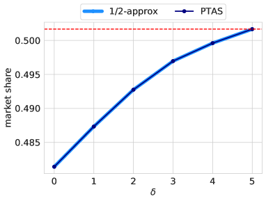
(a) The market share obtained by our algorithm under different levels of fairness constraints. The dashed line shows the optimal market share in the absence of fairness constraints.

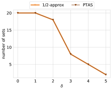
(b) The number of sets that our algorithms need to randomize over under different levels of fairness constraints.

Figure 5: The price introduced by fairness constraints in the MovieLens dataset.

1. Impact on the platform’s market share. Figure 5a shows the market share obtained by our algorithms under different levels of fairness constraints (i.e., $\delta$). The dashed line in this figure shows the average optimal market share in the absence of any fairness constraints, and hence it can be used to measure the price of fairness. As expected, we observe a clear tradeoff between fairness and market share. As the fairness constraint gets relaxed (i.e., as $\delta$ increases), the market share increases and approaches the maximum market share attainable in the absence of the fairness constraints. That being said, even when we require the platform to be $0$-fair ($\delta=0$), the price of fairness is quite small, as the average market share only gets reduced by around $4\%$ in our near-optimal solutions. This implies that we can achieve a high level of fairness in the movie recommendation platform without exerting a heavy impact on the market share.

2. Impact on the number of randomized sets. The introduction of the fairness constraints also requires us to randomize over a number of sets instead of sticking with a fixed assortment. Figure 5b plots the number of sets that we need to randomize over in our near-optimal solutions, under different levels of fairness constraints. We observe that the number of sets ranges from 1 to 20, highlighting that our algorithms can be effectively implemented in practice. Also, as $\delta$ increases and the fairness constraints get relaxed, the number of sets needed for randomization decreases.

Visibility. Recall that in Figure 3 of Section 4.3, we have previewed the visibility received by each movie (ranked in decreasing order of their qualities) given by the solution of our 1/2-approx. algorithm under different levels of fairness constraints. The plot shows that in general, the visibility of movies tends to decrease as their quality decreases (with slight variations due to the output coming from our approximate solutions). Additionally, in our approximate solution for each $\delta$, there is a rough threshold such that any movie with an index greater than this threshold gets positive visibility, while the remaining movies receive zero visibility. Note that this threshold decreases as $\delta$ increases, indicating that the parameter $\delta$ can be be effectively tuned to strike a balance between fairness (i.e., visibility of items with lower qualities) and the induced market share.

Runtime Comparison. Finally, we compare the computational performance of our $1/2$-approx. algorithm and PTAS. In Table 1, we record the runtime of these two algorithms. Here, the time taken by a single execution refers to the time taken to solve one instance of Problem (sub-dual($\mathbf{z},K$)). We need to solve many instances of Problem (sub-dual($\mathbf{z},K$)) throughout the run of the column generation method (see Section 13); hence, we also record the total time taken by our $1/2$-approx. algorithm and PTAS, when combined with the column generation method, to solve Problem (fair). We note that the $1/2$-approx. algorithm clearly outperforms the PTAS in terms of both the time required for a single execution and the total time taken to solve Problem (fair). This is expected, given their respective time complexities stated in Theorems 7.3 and 8.1. As the $1/2$-approx. algorithm is a subroutine of the PTAS and is called repeatedly during one execution of the PTAS, the latter is inherently slower. The superior computational performance of the $1/2$-approx. algorithm makes it an attractive practical option.

Table 1: Runtime comparison of $1/2$-approx. and PTAS algorithms on the MovieLens dataset.

	$\delta$	0	1	2	3	4	5
Time taken by a single execution (s)	$1/2$-approx	$7.1\times 10^{-2}$	$3.9\times 10^{-2}$	$3.7\times 10^{-2}$	$2.1\times 10^{-2}$	$1.4\times 10^{-2}$	$2.2\times 10^{-2}$
	PTAS	$4.2$	$2.9$	$2.8$	$1.6$	$7.6\times 10^{-1}$	$1.7$
Total time taken in solving (fair) (s)	$1/2$-approx	2.1	1.3	1.2	0.4	0.2	0.2
	PTAS	101.7	78.2	73.3	17.7	6.2	10.8

10 Conclusion and Future Directions

Many online platforms nowadays have largely relied on algorithms to optimize their operational decisions. However, the use of single-minded algorithms that are solely concerned about maximizing the platform’s expected revenue or market share can lead to an unfair outcome where the winner takes all. Motivated by this, we introduce the fair assortment planning problem, which involves a novel pairwise fairness notion that ensure items with similar qualities/merits receive similar outcomes. While many previous works on online operational decisions have focused on maximizing the utilities of the users or the platform, our work provides a new perspective that takes the interest of items on online platforms into account. This perspective is particularly important because an unfair allocation of user exposure would discourage many of the product sellers/contents creators/job candidates from remaining on the platform, which, as a result, will negatively impact the long-term prospect of the platform and narrow down users’ choices.

At a high level, in our work, we propose a novel framework that would give us access to a wide variety of near-optimal algorithms for our fair assortment planning problem. These near-optimal solutions require us to randomize over a polynomial number of assortments, which can be effectively implemented in practice. Theoretically, our PTAS attains an arbitrarily good approximation ratio, but we have also showed, via our case study in Section 9 and synthetic experiments in Section 16, that the $1/2$-approx. algorithm has outstanding computational performance and returns solutions with comparable quality. Another crucial insight from our case study is that in many real-world settings, a high level of fairness can in fact be achieved at a small cost to the platform; however, this would improve satisfaction among the sellers and in turn benefit the platform.

Our work opens up a number of new directions for future research. As discussed in Sections 3 and 4, our Ellipsoid-based framework and our approximate separation oracles used in this framework can be applied to different objective functions and a wide variety of pairwise notions of fairness. One natural direction is to further investigate how our unified, Ellipsoid-based framework works under other types of settings (e.g. different choice models, more constraints on the feasible set of assortments) that are of interest to real-world applications.

Another interesting research direction is to explore fair assortment planning problems in a dynamic setting. In our current model, we allocate outcomes to items in a single round based on their known qualities. It would be interesting to extend our approach to handle settings where the qualities or popularity of items are initially unknown and need to be learned by the algorithm. Moreover, the quality or popularity of items may evolve over time and depend on past assortment planning decisions. In such dynamic scenarios, it is crucial to ensure that fairness is preserved as we learn about the items’ attributes. Although we do not address this dynamic setting in our work, we believe that incorporating our fairness constraint could have long-term benefits and reduce the winner-takes-all phenomenon, which may manifest in dynamic scenarios. In sum, fairness has only been scarcely studied in operational decisions of online platforms, and we hope that this work would inspire a new stream of research in this area.

N.G. was supported in part by the MIT Indonesia seed grant. We thank Vivek Farias, Daniel Freund, Omar El Housni, Denis Sauré, Rad Niazadeh, and Edy Baskoro for their insightful comments during this work.

Appendices

11 An Example that Connects Our Fairness Notion with Alpha Fairness

We note that our proportional fairness notion in (2) can encompass the alpha fairness notion in certain cases. To see this, let us consider a simple assortment planning problem in which the platform can only present one item, i.e., $K=1$. Let $p_{i}$ denote the probability that the platform chooses to present item $i$. Suppose that the outcome received by item $i$ is its market share, i.e., $O_{i}=p_{i}\cdot(\frac{w_{i}}{1+w_{i}})$, and the quality of item $i$ is its probability of purchase if shown to the user, i.e., $q_{i}=\frac{w_{i}}{1+w_{i}}$.

Recall from Section 4.1 that the Nash bargaining solution achieves alpha fairness with $\alpha=1$. To obtain the Nash bargaining solution, we would maximize the social welfare function in Equation (3) for $\alpha=1$; that is, we maximize $\sum_{i\in[n]}\log{O_{i}}$ subject to the constraint $\sum_{i\in[n]}p_{i}=1$. The optimal solution that solves this problem satisfies $\frac{O_{i}}{q_{i}}=\frac{O_{i^{\prime}}}{q_{i^{\prime}}}$ for all $i\neq i^{\prime}$, which is precisely the fairness constraint we introduced in Equation (2) with $\delta=0$. In this case, the Nash bargaining solution can be seen as a special case that meets our fairness notion. Nonetheless, our fairness notion is much broader and can be applied to various situations, such as different types of outcomes $O_{i}$, various quality metrics $q_{i}$, and larger assortments; see Section 4.2 for a discussion on the generality of our fairness notion.

12 Details on the Ellipsoid Method

In this section, we provide more details on the Ellipsoid method used in Step 1 of the fair Ellipsoid-based algorithm, proposed in Section 5.3. Recall that in Section 5.3, we assume that we have access to a polynomial-time algorithm $\mathcal{A}$ that gives a $\beta$-approximate solution for Problem (sub-dual($\mathbf{z},K$)). We will use algorithm $\mathcal{A}$ within the Ellipsoid method, as part of our approximate separation oracle.

In Step 1 of the fair Ellipsoid-based algorithm, we apply the Ellipsoid method, outlined in Algorithm 3, to solve Problem (fair-dual). Here, we restate Problem (fair-dual):

$$\begin{aligned} \textsc{fair-dual}~{}=~{}\min_{\rho\geq 0,\mathbf{z}\geq\mathbf{0}}~{}~{}&\,\rho+\sum_{i=1}^{n}\sum_{j=1,j\neq i}^{n}\delta\cdot{q}_{i}q_{j}\cdot z_{ij}\\ \text{ s.t. }&\sum_{i\in S}\left(\sum_{j=1,j\neq i}^{n}(z_{ij}-z_{ji}){q}_{j}\right)+\rho\geq\textsc{rev}(S),\quad&\forall S:|S|\leq K\end{aligned}$$ (fair-dual)

For simplicity of notation, we can rewrite Problem (fair-dual) in the form of $\min\{\mathbf{d}^{\top}\mathbf{s}:\mathbf{A}\mathbf{s}\geq\mathbf{b},\mathbf{s}\geq 0\}$. Here, $\mathbf{s}=(\mathbf{z},\rho)\in\mathbb{R}^{n^{2}+1}$ is the vector of decision variables. $\mathbf{d}$ is a vector of size $n^{2}+1$ chosen such that $\mathbf{d}^{\top}\mathbf{s}=\rho+\sum_{i=1}^{n}\sum_{j=1,j\neq i}^{n}\delta\cdot{q}_{i}q_{j}\cdot z_{ij}$. $\mathbf{A}$ is a $N\times(n^{2}+1)$ matrix and $\mathbf{b}$ is a vector of size $N$, where $N=|\{S\subseteq[n]:|S|\leq K\}|$. Let each row of $\mathbf{A}$ and $\mathbf{b}$ be indexed by a set $S$ with $|S|\leq K$. The matrix $\mathbf{A}$ is chosen such that $\mathbf{a}_{S}^{\top}\mathbf{s}=\sum_{i\in S}\left(\sum_{j\in[n],j\neq i}(z_{ij}-z_{ji}){q}_{j}\right)+\rho$, where $\mathbf{a}_{S}$ is the row vector in $\mathbf{A}$ indexed by set $S$. The vector $\mathbf{b}$ is chosen such that $b_{S}=\textsc{rev}(S)$, where $b_{S}$ is component of $\mathbf{b}$ indexed by set $S$.

Within the Ellipsoid method, we keep track of the following quantities: (i) $(\mathbf{z},\rho)\in\mathbb{R}^{n^{2}+1}$, the center of the current ellipsoid, which is also the current solution to the dual problem; note that this solution might not be feasible for the dual problem. (ii) $(\mathbf{z}^{\star},\rho^{\star})$, the best feasible solution to the dual problem we have found so far. We initialize $(\mathbf{z}^{\star},\rho^{\star})$ to be $(\mathbf{0}_{n^{2}},1)$, where $\mathbf{0}_{n^{2}}$ is a zero vector of length $n^{2}$; this is always a feasible solution to Problem (fair-dual). (iii) the current best objective obj. We initialize it to be $1$, which is the objective of $(\mathbf{0}_{n^{2}},1)$. (iv) a positive-definite matrix $\mathbf{D}\in\mathbb{R}^{(n^{2}+1)\times(n^{2}+1)}$, which represents the shape of the ellipsoid. (v) a collection $\mathcal{V}$ of sets that have violated the dual fairness constraint during the execution of the Ellipsoid method.

Algorithm 3 The Ellipsoid method for Problem (fair-dual)

Input: Starting solution $(\mathbf{z}_{0},\rho_{0})$, starting matrix $\mathbf{D}_{0}$, maximum number of iterations $t_{\max}$, a $\beta$-approx. algorithm $\mathcal{A}$ for Problem (sub-dual($\mathbf{z},K$)). Here, we rewrite Problem (fair-dual) in the form of $\min\{\mathbf{d}^{\top}\mathbf{s}:\mathbf{A}\mathbf{s}\geq\mathbf{b},\mathbf{s}\geq 0\}$. The matrix $\mathbf{A}$ is chosen such that $\mathbf{a}_{S}^{\top}\mathbf{s}=\sum_{i\in S}\left(\sum_{j\in[n],j\neq i}(z_{ij}-z_{ji}){q}_{j}\right)+\rho$, where $\mathbf{a}_{S}$ is the row vector in $\mathbf{A}$ indexed by set $S$. The vector $\mathbf{b}$ is chosen such that $b_{S}=\textsc{rev}(S)$, where $b_{S}$ is component of $\mathbf{b}$ indexed by set $S$.
Output: (i) A collection $\mathcal{V}$ of sets that have violated constraints. (ii) An optimal, feasible solution $(\mathbf{z}^{\star},\rho^{\star})\geq 0$ (iii) optimal objective obj.

1. Initialization. $(\mathbf{z},\rho)=(\mathbf{z}_{0},\rho_{0}),(\mathbf{z}^{\star},\rho^{\star})=(0,1),\textsc{obj}=1,\mathbf{D}=\mathbf{D}_{0},\mathcal{V}=\emptyset,$ and $t=0$.

2. While $t\leq t_{\max}$:

   1. Find a violated constraint.

      • Check if we can reduce the objective further. If $\rho+\sum_{i=1}^{n}\sum_{j=1,j\neq i}\delta\cdot{q}_{i}q_{j}\cdot z_{ij}^{n}\geq\textsc{obj}$, set $\mathbf{a}=-\mathbf{d}$ and go to Step 2(b).

      • Check if the non-negativity constraints hold. If $\rho<0$, set $\mathbf{a}=\mathbf{e}_{n^{2}+1}$; else if $z_{ij}<0$ for some $(i,j)$, set $\mathbf{a}=\mathbf{e}_{i\cdot n+j}$, where $\mathbf{e}_{k}$ is the unit vector with a $1$ in the $k$th coordinate. Go to Step 2(b).

      • Check if the dual fairness constraints holds using the approximate separation oracle.

        • Apply the $\beta$-approximate algorithm $\mathcal{A}$ to Problem (sub-dual($\mathbf{z},K$)) that returns $S_{\mathcal{A}}$ with $|S_{\mathcal{A}}|\leq K$ such that $\textsc{rev-cost}(S_{\mathcal{A}},\mathbf{z})\geq\beta\cdot\textsc{sub-dual}(\mathbf{z},K)$.

        • If $\textsc{rev-cost}(S_{\mathcal{A}},\mathbf{z})>\rho$, then set $S_{\mathcal{A}}$ is violating the constraint. Set $\mathbf{a}=\mathbf{a}_{S}$ and add $S_{\mathcal{A}}$ to $\mathcal{V}$.

      • If we have found no violated constraint, update our best feasible solution and its objective:

        $$(\mathbf{z}^{\star},\rho^{\star})\leftarrow(\mathbf{z},\rho)\quad\text{and}\quad\textsc{obj}\leftarrow\rho^{\star}+\sum_{i=1}^{n}\sum_{j=1,j\neq i}^{n}\delta\cdot{q}_{i}q_{j}\cdot z^{\star}_{ij}\,.$$

        Then, go back to the start of Step 2 and re-enter the while loop.

   2. Use the violated constraint to decrease the volume of the ellipsoid and find a new solution.

      $$(\mathbf{z},\rho) \leftarrow(\mathbf{z},\rho)+\frac{1}{n^{2}+2}\frac{\mathbf{D}\mathbf{a}}{\sqrt{\mathbf{a}^{\top}\mathbf{D}\mathbf{a}}}\,;$$

      $$\mathbf{D} \leftarrow\frac{(n^{2}+1)^{2}}{(n^{2}+1)^{2}-1}\Big{(}\mathbf{D}-\frac{2}{n^{2}+2}\frac{\mathbf{D}\mathbf{a}\mathbf{a}^{\top}\mathbf{D}}{\mathbf{a}^{\top}\mathbf{D}\mathbf{a}}\Big{)}\,.$$

   3. $t\leftarrow t+1\,.$

3. The ellipsoid is sufficiently small. Return $\mathcal{V},(\mathbf{z}^{\star},\rho^{\star}),\textsc{obj}$.

At a high level, the Ellipsoid method for Problem (fair-dual) (Algorithm 3) works in the following way. At each iteration, it generates an ellipsoid $E$ centered at the current solution $\mathbf{s}=(\mathbf{z},\rho)$, which is defined as:

$$E=\{\mathbf{x}:(\mathbf{x}-\mathbf{s})^{\top}\mathbf{D}^{-1}(\mathbf{x}-\mathbf{s})\leq 1\}\,.$$

By design of the Ellipsoid method, the ellipsoid $E$ always contains the intersection of the feasibility region of Problem (fair-dual) and the half space $\{\mathbf{s}:\mathbf{d}^{\top}\mathbf{s}<\textsc{obj}\}$.

In Step 2(a), the algorithm first attempts to check if the current solution is feasible and improves our objective, via finding a violated constraint. There are three types of violated constraints that we consider: (i) the objective constraint is violated if the current solution $(\mathbf{z},\rho)$ does not yield an objective less than obj; (ii) the non-negativity constraint is violated if any of the entries in $(\mathbf{z},\rho)$ is negative; (iii) the dual fairness constraint is violated if we can find a set $S$ with $|S|\leq K$ such that $\textsc{rev-cost}(S,\mathbf{z})>\rho$. Note that when examining the dual fairness constraint, instead of examining the dual fairness constraint for every $S$ such that $|S|\leq K$, we instead use an approximate separation oracle that relies on algorithm $\mathcal{A}$. First, it applies the $\beta$-approximate algorithm $\mathcal{A}$ to Problem (sub-dual($\mathbf{z},K$)), and gets $S_{\mathcal{A}}$ with $|S_{\mathcal{A}}|\leq K$ such that $\textsc{rev-cost}(S_{\mathcal{A}},\mathbf{z})\geq\beta\cdot\textsc{sub-dual}(\mathbf{z},K)$. Then, if $\textsc{rev-cost}(S_{\mathcal{A}},\mathbf{z})>\rho$, set $S_{\mathcal{A}}$ has violated the dual fairness constraint. Otherwise, the solution $(\mathbf{z},\rho)$ is declared feasible. In the proof of Theorem 5.3, we will show that the use of the approximate separation oracle might cause the solution $(\mathbf{z}^{\star},\rho^{\star})$ returned by the Ellipsoid method to be infeasible for Problem (fair-dual); however, the objective obj returned by the Ellipsoid method would stay close to the true optimal objective fair-dual.

If we have found one of the constraints violated in Step 2(a), which can be written as $\mathbf{a}^{\top}\mathbf{s}<b$ for some $\mathbf{a}\in\mathbb{R}^{n^{2}+1}$ and $b\in\mathbb{R}$, we then go to Step 2(b) and construct a new ellipsoid $E^{\prime}$. We do so by updating the center of the ellipsoid $(\mathbf{z},\rho)$ and the positive-definite matrix $\mathbf{D}$ that defines our ellipsoid; see Step 2(b) (with slight differences in notations).

$$(\mathbf{z}^{\prime},\rho^{\prime})\leftarrow(\mathbf{z},\rho)+\frac{1}{n^{2}+2}\frac{\mathbf{D}\mathbf{a}}{\sqrt{\mathbf{a}^{\top}\mathbf{D}\mathbf{a}}}\quad\text{and}\quad\mathbf{D}^{\prime}\leftarrow\frac{(n^{2}+1)^{2}}{(n^{2}+1)^{2}-1}\Big{(}\mathbf{D}-\frac{2}{n^{2}+2}\frac{\mathbf{D}\mathbf{a}\mathbf{a}^{\top}\mathbf{D}}{\mathbf{a}^{\top}\mathbf{D}\mathbf{a}}\Big{)}\,.$$

The volume of the new ellipsoid $E^{\prime}$ defined by $(\mathbf{z}^{\prime},\rho^{\prime})$ and $\mathbf{D}^{\prime}$ is only a fraction of the volume of the previous ellipsoid $E$. In addition, this new ellipsoid has a new center $\mathbf{s}^{\prime}=(\mathbf{z}^{\prime},\rho^{\prime})$ that satisfies $\mathbf{a}^{\top}\mathbf{s}^{\prime}>\mathbf{a}^{\top}\mathbf{s}$. We then start a new iteration, in which we check whether the new solution $(\mathbf{z}^{\prime},\rho^{\prime})$ is feasible and improves our objective.

On the other hand, if we have found no violated constraint, this means that our current solution $(\mathbf{z},\rho)$ is (approximately) feasible and also improves the objective obj obtained by the previous best feasible solution $(\mathbf{z}^{\star},\rho^{\star})$. If this happens, we then set the current solution to be our current best feasible solution, i.e., $(\mathbf{z}^{\star},\rho^{\star})\leftarrow(\mathbf{z},\rho)$, and update the current optimal objective obj to be the objective obtained by the current solution. Then, we start a new iteration by re-entering Step 2, and seeks to find a feasible solution that can further reduce our objective function.

The Ellipsoid method for Problem (fair-dual) terminates when the ellipsoid $E$ is sufficiently small, by selecting a sufficiently large $t_{\max}$. Recall that the ellipsoid $E$ always contains the intersection of the feasibility region of Problem (fair-dual) and the half space $\{\mathbf{s}:\mathbf{d}^{\top}\mathbf{s}<\textsc{obj}\}$. Intuitively, when the ellipsoid gets reduced to a sufficiently small volume, it is unlikely that there exists a feasible solution that can further reduce our objective. It is shown, in Bertsimas and Tsitsiklis [1997], that given a separation oracle, the Ellipsoid method is guaranteed to terminate in $t_{\max}=\mathcal{O}(n^{12}\log(nq_{\max}))$ iterations, where $q_{\max}$ is the the maximum adjusted measurement of quality (see definition in Section 5.3). When the Ellipsoid method terminates, it returns the following: (i) the collection $\mathcal{V}$ of sets that have violated the dual fairness constraint; (ii) the optimal solution $(\mathbf{z}^{\star},\rho^{\star})$ and (iii) the optimal objective obj. Note that this collection $\mathcal{V}$ would then play an important role in Step 2 of the fair Ellipsoid-based algorithm. As discussed in Section 5.3, we then use the collection $\mathcal{V}$ to reduce the number of variables to be considered in the primal problem (fair) to a polynomial size.

13 Details on the Column Generation Method

In this section, we provide a brief description of the column generation method for Problem (fair) (see Bertsimas and Tsitsiklis [1997] for more information on this method). We have employed this method, in combination with our approximation algorithms (1/2-approx. algorithm and PTAS) for Problem (sub-dual($\mathbf{z},K$)), to numerically solve the fair assortment planning problems in Sections 9 and 16. While there is no polynomial-time guarantee for the column generation method, it is often computationally efficient in practice and serves as a viable alternative to the fair Ellipsoid-based framework proposed in Section 5.3, which theoretically establishes that Problem (fair) can be solved near-optimally in polynomial time.

In Algorithm 4, we outline the column generation method for Problem (fair). At a high level, the column generation considers two optimization problems—a master problem and a subproblem. The master problem is a simplified version of the original optimization problem, which, in our case, is Problem (fair), restricted to a subset of variables. The subproblem is a new problem that identifies one additional variable that we can consider in the master problem, which would further improve the objective function. In our case, the subproblem reduces to solving Problem (sub-dual($\mathbf{z},K$)).

Algorithm 4 Column generation method for Problem (fair)

Input: Problem instance $\Theta=(\mathbf{a},\mathbf{b},\mathbf{r},\mathbf{w},\mathbf{q})$, a $\beta$-approx. algorithm $\mathcal{A}$ for Problem (sub-dual($\mathbf{z},K$)).
Output: A $\beta$-approximate solution $\widehat{p}(S)$ to Problem (fair).

1. Initialization. Initialize the collection of sets to include only sets with size one: $\mathcal{V}=\Big{\{}\{1\},\dots,\{n\}\Big{\}}$.

2. Repeatedly solve the master and the subproblem until the stopping rule is satisified.

   1. Solve the master problem. Solve Problem (fair) with $p(S)=0$ for all $S\notin\mathcal{V}$, which returns primal solution $\widehat{p}(S)$ and dual solution $(\mathbf{{z}},{\rho})$.

   2. Solve the subproblem. Apply the $\beta$-approximate algorithm $\mathcal{A}$ to solving Problem (sub-dual($\mathbf{z},K$)), which returns $S_{\mathcal{A}}$ with $|S_{\mathcal{A}}|\leq K,S_{\mathcal{A}}\notin\mathcal{V}$ such that $\textsc{rev-cost}(S_{\mathcal{A}},\mathbf{z})\geq\beta\cdot\textsc{sub-dual}(\mathbf{z},K)$.

   3. Check whether $S_{\mathcal{A}}$ can improve the objective of Problem (fair)

      • If $\textsc{rev-cost}(S_{\mathcal{A}},\mathbf{z})>\rho$, then set $S_{\mathcal{A}}$ is an improving variable. Add $S_{\mathcal{A}}$ to $\mathcal{V}$ and go back to Step 2(a).

      • Stopping rule. If $\textsc{rev-cost}(S_{\mathcal{A}},\mathbf{z})\leq\rho$, return the solution $\widehat{p}(S)$.

At each iteration of the column generation method, we first solve the master problem, i.e., Problem (fair), with only a subset of variables under consideration. That is, we only consider a restricted collection of sets $\mathcal{V}\subset\{S\subset[n]:|S|\leq K\}$ when solving Problem (fair), and let $p(S)=0$ for all $S\notin\mathcal{V}$. We then need to solve a subproblem to determine if there is an additional set $S\notin\mathcal{V}$ that we wish to consider, in order to improve the objective of Problem (fair). To do that, we can simply compute the reduced cost associated with each $S$ such that $S\notin\mathcal{V}$ (see Section 24 for a formal definition of the reduced cost) and pick the set $S$ with the highest reduced cost. Given problem instance $\Theta=(\mathbf{a},\mathbf{b},\mathbf{r},\mathbf{w},\mathbf{q})$ and the dual variables $(\mathbf{z},\rho)$, the reduced cost $C_{S}$ associated with each set $S\notin\mathcal{V}$ is:

$$\bar{C}_{S}=\textsc{rev-cost}(S,\mathbf{z})-\rho\,.$$

Hence, if we found $S\notin\mathcal{V}$ such that $\textsc{rev-cost}(S,\mathbf{z})>\rho$, adding it to the collection $\mathcal{V}$ and resolving Problem (fair) would allow us to obtain a better objective. On the other hand, if there exists no set $S\notin\mathcal{V}$ with a positive reduced cost (i.e., $\textsc{rev-cost}(S,\mathbf{z})\leq\rho$ for all $S\notin\mathcal{V}$, the optimality conditions of Problem (fair) are satisfied (see Section 24) and the current solution of Problem (fair) is optimal. In Algorithm 4, in order to solve the subproblem and find the set $S$ with the highest reduced cost, we apply a $\beta$-approximate algorithm $\mathcal{A}$ for Problem (sub-dual($\mathbf{z},K$)), which returns a $\beta$-approximate solution $S_{\mathcal{A}}$ for $\max_{S:|S|\leq K}\textsc{rev-cost}(S,\mathbf{z})$. We then compare $\textsc{rev-cost}(S_{\mathcal{A}},\mathbf{z})$ with the dual variable $\rho$: (i) if $\textsc{rev-cost}(S_{\mathcal{A}},\mathbf{z})>\rho$, adding $S_{\mathcal{A}}$ to the collection $\mathcal{V}$ and resolving Problem (fair) would improve the objective; (ii) otherwise, we simply terminate our algorithm and return the current solution.

Using the same proof presented in Segment 1 of proof for Theorem 5.3, it can be shown that Algorithm 4, utilizing the column generation method, returns a $\beta$-approximate feasible solution $\widehat{p}(S),S\subset[n]$, to Problem (fair). Since the number of columns (variables) is finite, the column generation method is also guaranteed to terminate in finite, but not necessarily polynomial, number of iterations.

14 Extensions of the $1/2$-Approx. Algorithm

We present two extensions of the $1/2$-approx. algorithm (Algorithm 1) introduced in Section 7. In Section 14.1, we focus on visibility-fair instances with uniform revenues, and present a $1/2$-approx. algorithm for $\max_{W\geq 0}\textsc{kp}(W,K)$ (Algorithm 5) with improved runtime. In Section 14.2, we present a modified version of the $1/2$-approx. algorithm, which serves as an subroutine of the PTAS (Algorithm 2) in Section 8.

14.1 $1/2$-Approx. Algorithm for Problem (sub-dual($\mathbf{z},K$)) in Visibility-Fair Instances with Uniform Revenues

In this section, we focus our attention on visibility-fair instances with uniform revenues. That is, we consider a problem instance $\Theta=(0,\mathbf{b},\mathbf{r},\mathbf{w},\mathbf{q})$ where all items have the same revenues, i.e., $r_{i}=r$ for all $i\in[n]$. Recall from Section 3 that the assumption of uniform revenues is of interest to platforms that seek to maximize their market share, or those that adopt a fixed commission model.

We first note that even in visibility-fair instances with uniform revenues, Problem (sub-dual($\mathbf{z},K$)) remains NP-complete (see Theorem 5.2), and approximation algorithms are needed. However, such instances also come with the special structure that the post-fairness revenues for all items are homogeneous, i.e., $\mathcal{r}_{i}=r$ for all $i\in[n]$, which results in the potential of further improving the runtime of our approximation algorithms. In the rest of this section, we will present a simplified version of the $1/2$-approx. algorithm for Problem (sub-dual($\mathbf{z},K$)) that enjoys a better time complexity. In Section 15, we will also present an FPTAS for Problem (sub-dual($\mathbf{z},K$)) in visibility-fair instances with uniform revenues.

Our $1/2$-approx. algorithm for $\max_{W\in I}~{}\textsc{kp}(W,K)$ in a visibility-fair instance with uniform revenues is presented in Algorithm 5. Its procedure is very similar to that in Algorithm 1 with slight modifications. The key idea here is that when all items have the same post-fairness revenues, we no longer need to pre-partition the interval $[0,\infty)$ into $\mathcal{O}(n^{3})$ well-behaving sub-intervals, as done in Section 7.2. Instead, we can directly apply Algorithm 5 to the interval $[0,\infty)$.

Algorithm 5 $\mathcal{A}_{1/2}^{u}(\mathbf{w},r,\mathbf{\mathfrak{c}},K)$: $1/2$-approx. algorithm for $\max_{W\geq 0}~{}\textsc{kp}(W,K)$ in a visibility-fair instance with uniform revenues

Input: weights $\mathbf{w}=\{w_{i}\}_{i\in[n]}$, revenue $r$, post-fairness costs $\mathbf{\mathfrak{c}}=\{\mathfrak{c}_{i}\}_{i\in[n]}$, and cardinality upper bound $K$.
Output: collection of sets $\mathcal{C}$ and assortment $S_{1/2}$.

1. Initialization.

   1. Initialize the collection of assortments $\mathcal{C}=\emptyset$. For $j\in[n]$, add $\{j\}$ to $\mathcal{C}$.

   2. Rank the items by their utility-to-weight ratios. Let $h_{j}$ be the index of the item with the $j$th highest utility-to-weight ratio, and define $H_{j}=\{h_{1},\dots,h_{j}\}$, for $j\in[K]$ and $W_{\textsc{TH}}=w(H_{K})$.

2. Interval $I_{\text{low}}=[0,W_{\textsc{TH}})$.

   1. For $j=1,\dots,K$, add $H_{j}$ to $\mathcal{C}$.

   2. Stopping rule. If $u_{h_{K}}(W_{\textsc{TH}})\geq 0$, go to Step 3; otherwise, go to Step 4 (i.e., the termination step).

3. Interval $I_{\text{high}}=[W_{\textsc{TH}},\infty)$.

   1. Initialize the profile. Set $P_{1}=H_{K},P_{0}=[n]\setminus H_{K}$, and $W_{\text{next}}=W_{\textsc{TH}}$.

   2. Adaptively partitioning $I_{\text{high}}$. While there exist $i\in P_{1},j\in P_{0}$ such that $w_{i}<w_{j}$:

      1. Update $W_{\text{next}}$ and the indices $\textsf{i}^{\star},\textsf{j}^{\star}$ as follows:

         $$(\textsf{i}^{\star},\textsf{j}^{\star})\leftarrow\mathop{\rm arg\,min}_{i\in P_{1},j\in P_{0}\atop{w_{i}<w_{j}}}\dfrac{\mathfrak{c}_{j}-\mathfrak{c}_{i}}{w_{j}-w_{i}},\qquad\text{and}\qquad W_{\text{next}}\leftarrow W_{\text{next}}-w_{\textsf{i}^{\star}}+w_{\textsf{j}^{\star}}\,.$$

      2. Swapping the two items. Set $P_{1}\leftarrow P_{1}\cup\{\textsf{j}^{\star}\}\setminus\{\textsf{i}^{\star}\}$ and $P_{0}\leftarrow P_{0}\cup\{\textsf{i}^{\star}\}\setminus\{\textsf{j}^{\star}\}$.

      3. Stopping rule. If $\dfrac{\mathfrak{c}_{\textsf{j}^{\star}}-\mathfrak{c}_{\textsf{i}^{\star}}}{w_{\textsf{j}^{\star}}-w_{\textsf{i}^{\star}}}\leq\dfrac{r}{1+W_{\text{next}}}$, add $P_{1}$ to $\mathcal{C}$. Otherwise, go to the termination Step 4.

4. Termination Step. Return the collection $\mathcal{C}$ and assortment $S_{1/2}=\mathop{\rm arg\,max}_{S\in\mathcal{C}}\textsc{rev-cost}(S,\mathbf{z})$.

Using a proof similar to that of Theorem 7.3, we can show the following result for Algorithm 5. Here, the runtime complexity is improved by $\mathcal{O}(n^{3})$ compared to Theorem 7.3.

Corollary 14.1 ($1/2$-Approx. Algorithm for a Visibility-Fair Instance with Uniform Revenues)

Given a visibility-fair instance $\Theta=(0,\mathbf{b},\mathbf{r},\mathbf{w},\mathbf{q})$ with uniform revenues $r_{i}=r\in(0,\bar{r}]$ for all $i\in[n]$. For any $\mathbf{z}\geq\mathbf{0}$, if Algorithm 5 returns collection $\mathcal{C}$ and set $S_{1/2}$, we have that for any $W\in[0,\infty)$, there exists a set $S\in\mathcal{C}$ such that

$$\textsc{rev-cost}(S,\mathbf{z})\geq\frac{1}{2}~{}\textsc{kp}(W,K)\,.$$

In particular, the set $S_{1/2}$ satisfies

$$\textsc{rev-cost}(S_{1/2},\mathbf{z})\geq\frac{1}{2}\max_{W\in[0,\infty)}~{}\textsc{kp}(W,K)\,.$$

Given Algorithm 5, the overall complexity to find a $1/2$-approx. solution for $\max_{W\geq 0}\textsc{kp}(W,K)$ is in the order of $\mathcal{O}(n^{2}\log n+nK^{2})$.

To see why we can improve runtime complexity by $\mathcal{O}(n^{3})$, observe that in visibility-fair instances with uniform revenues $r$, all items have the same post-fairness revenues, i.e., $\mathcal{r}_{i}=r_{i}-a_{i}c_{i}=r$ for all $i\in[n]$. In this case, we no longer need to pre-partition the interval $[0,\infty)$ into $\mathcal{O}(n^{3})$ well-behaving sub-intervals according to Definition 7.2. Conditions (i) and (ii) in Definition 7.2 can be taken care of via slightly modifying Step 3 (see modifications in Algorithm 5). Condition (iii) and (iv) in Definition 7.2, on the other hand, are naturally implied by $\mathcal{r}_{i}=r$ for all $i\in[n]$. To see that, note that when $\mathcal{r}_{i}=r$ for any $i\in[n]$, the utility-to-weight ratio of item $i\in[n]$ is

$$\frac{u_{i}(W)}{w_{i}}=\frac{\frac{rw_{i}}{1+W}-\mathfrak{c}_{i}}{w_{i}}=\frac{r}{1+W}-\frac{\mathfrak{c}_{i}}{w_{i}}\,.$$

The ordering of utility-to-weight ratios of items hence no longer depends on the value of $W$, which suggests that condition (iii) holds. Similarly, fix an item $i\in[n]$ in the knapsack, we can also compute the marginal increase in utility if we replace item $i$ with another item $j\neq i$ that is not in the knapsack:

$$\frac{u_{j}(W)-u_{i}(W)}{w_{j}-w_{i}}=\frac{(\frac{rw_{j}}{1+W}-\mathfrak{c}_{j})-(\frac{rw_{i}}{1+W}-\mathfrak{c}_{i})}{w_{j}-w_{i}}=\frac{r}{1+W}-\frac{\mathfrak{c}_{j}-\mathfrak{c}_{i}}{w_{j}-w_{i}}\,.$$

Clearly, the ordering of the term $\frac{u_{j}(W)-u_{i}(W)}{w_{j}-w_{i}}$ for any $j\neq i$ also does not depend on the values of $W$, hence implying that condition (iv) holds.

From a high level, when the items have different post-fairness revenues $\mathcal{r}_{i}$’s, the changes in the values of $W$ can influence the utility of each item in a highly heterogeneous fashion. Our pre-partitioning step thus ensures that the nature of our knapsack problem does not change too drastically on each well-behaving interval. In visibility-fair instances with uniform revenues, however, the homogeneity of the post-fairness revenues ensures that changes in the values of $W$ influence all items in the same way. This allows us to perform the adaptive partitioning procedure on the interval $[0,\infty)$ directly, leading to an improved runtime.

14.2 A Modified $1/2$-Approx. Algorithm as a Subroutine of PTAS

In Algorithm 6, we present another modified version of the $1/2$-approx. algorithm (Algorithm 1) presented in Section 7, which we would use as a subroutine of our PTAS (Algorithm 2). Given a well-behaving sub-interval $I\in[0,\infty)$ and some subset $L\subset[n]$ with fixed size $\ell$, Algorithm 6 is designed to solve a series of sub-knapsack problems, $\textsc{kp-sm}(W,K,L)$, for any $W\in I$. Here, $\textsc{kp-sm}(W,K,L)$ is a sub-knapsack problem defined on $\textsc{sm}(L)$:

$$\textsc{kp-sm}(W,K,L)=\max_{S\subseteq\textsc{sm}(L)}\sum_{i\in S}u_{i}(W)\quad\text{ s.t. }\sum_{i\in S}w_{i}\leq W-w(L)\quad\text{and}\quad|S|\leq K-\ell\,,$$

where

$$\textsc{sm}(L)=\Big{\{}i\in[n]\setminus L:u_{i}(W)\leq\min_{j\in L}\left\{u_{j}(W)\right\}\text{ for any $W\in I$}\Big{\}}\,.$$

To intuitively understand what the sub-knapsack problem $\textsc{kp-sm}(W,K,L)$ stands for, consider the setting when we have already added the set $L$ to a knapsack of capacity level $W$ and cardinality upper bound $K$, and we would like to add some more items from $\textsc{sm}(L)$ to the knapsack. Solving $\textsc{kp-sm}(W,K,L)$ helps us determine which of the items from $\textsc{sm}(L)$ to add so that we can maximize the total utilities of the knapsack.

Our modified $1/2$-approx. algorithm (Algorithm 6) only differs slightly from the original $1/2$-approx. algorithm (Algorithm 1), where the modifications enable us to only work with items in $\textsc{sm}(L)$ as we solve the series of sub-knapsack problems $\textsc{kp-sm}(W,K,L)$. The main procedures of the algorithm remains the same. In Algorithm 6, we highlight the parts where it differs from Algorithm 1.

Algorithm 6 $\tilde{\mathcal{A}}_{1/2}(L,\textsc{sm}(L),K,I)$: Modified $1/2$-approx. algorithm for $\textsc{kp-sm}(W,K,L)$

Input: A set $L$ with size $|L|=\ell$ and total weight $w(L)$, a set of items $\textsc{sm}(L)$ defined in Equation (8), weights $\mathbf{w}=\{w_{i}\}_{i\in\textsc{sm}(L)}$, post-fairness revenues $\mathbf{\mathcal{r}}=\{\mathcal{r}_{i}\}_{i\in\textsc{sm}(L)}$, post-fairness costs $\mathbf{\mathfrak{c}}=\{\mathfrak{c}_{i}\}_{i\in\textsc{sm}(L)}$, cardinality upper bound $K$, a well-behaving interval $I=[W_{\min},W_{\max})\subset[0,\infty)$ per Definition 7.2.
Output: a collection of assortment $\mathcal{C}_{1/2}(L)$ that includes a $1/2$-approx. assortment for $\max_{W\in I}\textsc{kp-sm}(W,K,L)$.

1. Initialization.

   1. Rank the items in $\textsc{sm}(L)$ by their utility-to-weight ratios. Let $h_{j}$ be the index of the item with the $j$th highest utility-to-weight ratio, for $j\in\textsc{sm}(L)$. Let $d=\min\{|\textsc{sm}(L)|,K-\ell\}$, and define $H_{j}=\{h_{1},\dots,h_{j}\}$, for $j\leq d$ and $W_{\textsc{TH}}=w(H_{d})+w(L)$.  // Note that $W_{\textsc{TH}}$ is defined differently.

   2. Initialize the collection of assortments $\mathcal{C}_{1/2}(L)=\emptyset$. For $j\in\textsc{sm}(L)$, add $\{j\}$ to $\mathcal{C}_{1/2}(L)$.

2. Interval $I_{\text{low}}=I\cap[0,W_{\textsc{TH}})$. If $I_{\text{low}}$ is non-empty:

   1. For $j=1,\dots,d$, add $H_{j}$ to $\mathcal{C}_{1/2}(L)$.

   2. Stopping rule. If $u_{h_{d}}(W_{\textsc{TH}})\geq 0$ with $d=K-\ell$, go to Step 3; otherwise, go to Step 4 (i.e., the termination step).

3. Interval $I_{\text{high}}=I\cap[W_{\textsc{TH}},\infty)$. If $I_{\text{high}}$ is non-empty:

   1. Initialize the profile.  // Note that the items in the profile are from $\textsc{sm}(L)$.

      • If $W_{\min}\leq W_{\textsc{TH}}$, set $P_{1}=H_{d},P_{0}=\textsc{sm}(L)\setminus H_{d}$, and $W_{\text{next}}=W_{\textsc{TH}}$.

      • If $W_{\min}>W_{\textsc{TH}}$, compute an optimal basic solution for LP relaxation of Problem $(\textsc{kp-sm}(W_{\min},K,L))$, which has profile $\{P_{1}(W_{\min}),(\textsf{i},\textsf{j}),P_{0}(W_{\min})\}$. Add $P_{1}(W_{\min})\cup\{\textsf{i}\}$ and $P_{1}(W_{\min})\cup\{\textsf{j}\}$ to $\mathcal{C}_{1/2}(L)$. Set $P_{1}=P_{1}(W_{\min})\cup\{\textsf{j}\}$, $P_{0}=\textsc{sm}(L)\setminus P_{1}$, and $W_{\text{next}}=w(P_{1})+w(L)$.

   2. Adaptively partitioning $I_{\text{high}}$. While there exist $i\in P_{1},j\in P_{0}$ such that $w_{i}<w_{j}$:

      1. Update indices $\textsf{i}^{\star},\textsf{j}^{\star}$ as follows:

         $$(\textsf{i}^{\star},\textsf{j}^{\star})\leftarrow\mathop{\rm arg\,max}_{i\in P_{1},j\in P_{0}\atop{w_{i}<w_{j}}}\left[\frac{u_{j}(W_{\text{next}})-u_{i}(W_{\text{next}})}{w_{j}-w_{i}}\right]\,.$$

      2. Stopping rule. If $W_{\text{next}}\geq W_{\text{max}}$ or $u_{\textsf{i}^{\star}}(W_{\text{next}})>u_{\textsf{j}^{\star}}(W_{\text{next}})\,,$ go to Step 4.

      3. Swapping the two items. Update $P_{1},P_{0},W_{\text{next}}$ as follows:

         $$P_{1}\leftarrow P_{1}\cup\{\textsf{j}^{\star}\}\setminus\{\textsf{i}^{\star}\}\quad\text{and}\quad P_{0}\leftarrow P_{0}\cup\{\textsf{i}^{\star}\}\setminus\{\textsf{j}^{\star}\}\quad\text{and}\quad W_{\text{next}}\leftarrow W_{\text{next}}-w_{\textsf{i}^{\star}}+w_{\textsf{j}^{\star}}\,.$$

         Add $P_{1}$ to $\mathcal{C}_{1/2}(L)$.

4. Termination Step. Return the collection $\mathcal{C}_{1/2}(L)$.

Using a proof similar to that of Theorem 7.3, we can show the following result for Algorithm 6.

Corollary 14.2 (Modified $1/2$-Approx. Algorithm for $(\textsc{KP-SM}(W,K,L))$)

Consider any interval $I\subset[0,\infty)$ that is well-behaving per Definition 7.2. For any $\mathbf{z}\geq\mathbf{0}$, and given some subset $L\subset[n]$, if Algorithm 6 returns collection $\mathcal{C}_{1/2}(L)$, we have that for any $W\in I$, there exists a set $S\in\mathcal{C}_{1/2}(L)$ such that

$$\textsc{rev-cost}(S,\mathbf{z})\geq\frac{1}{2}~{}\textsc{kp-sm}(W,K,L)\,.$$

Further, the overall complexity of Algorithm 6 is in the order of $\mathcal{O}(n^{2}\log n+nK^{2})$.

15 FPTAS for Problem (sub-dual($\mathbf{z},K$)) in a Visibility-Fair Instance with Uniform Revenues

In this section, we focus on a special case of Problem (sub-dual($\mathbf{z},K$)), for which approximation algorithms with even stronger theoretical guarantee (an FPTAS) is achievable. In particular, we consider a visibility-fair instance, where the instance takes the form $\Theta=(0,\textbf{b},\textbf{r},\textbf{w},\textbf{q})$, where all items generate uniform revenues $r$. (Problem (sub-dual($\mathbf{z},K$)) in such a instance is also NP-complete; see Theorem 5.2.) We will show that in such instances, it is possible to design an FPTAS fair Ellipsoid-based algorithm for Problem (sub-dual($\mathbf{z},K$)), which returns a $(1-\epsilon)$-approximate solution for any $\epsilon>0$, with polynomial runtime in not only $n$ and $K$, but also $1/\epsilon$. This, along with our Ellipsoid-based framework in Section 5.3, then leads to an FPTAS Ellipsoid-based algorithm for Problem (fair).

In the rest of this section, let $r_{i}=r$ for all $i\in[n]$. As we briefly discussed in Section 3, the assumption of uniform revenues is of particular interest to platforms that aim to maximize their market share (e.g., social media or job recommendation sites), or those that adopt a fixed commission model. Recall also from our discussion in Section 14.1 that since we consider a visibility-fair instance where $\mathbf{a}=0$, we also have post-fairness revenue $\mathcal{r}_{i}=r_{i}-a_{i}c_{i}=r$ for all $i\in[n]$.

Similar to what we did in Sections 7 and 8, the design of this FPTAS relies on transforming Problem (sub-dual($\mathbf{z},K$)) to $\max_{W\geq 0}~{}\textsc{kp}(W,K)$, as shown in Theorem 6.2. However, we will show in this section how to take further advantage of the special structure of having uniform revenues across all items to achieve better runtime than the PTAS presented in Section 8.

The FPTAS we propose draws inspiration from the FPTAS developed in Caprara et al. [2000]. The authors proposes an FPTAS for a single knapsack problem with cardinality constraint, which uses a dynamic programming (DP) scheme. In our problem, however, one main difficulty is that we need to solve an infinite number of parameterized knapsack problems with a cardinality constraint, where parameter $W\in[0,\infty)$ determines the capacity of the knapsack and also influences the utilities of the items. This further leads to a number of new challenges: (i) it is unrealistic to apply the aforementioned DP approach to every $W\in[0,\infty)$ as there are infinite number of them; (ii) in the FPTAS for a single knapsack problem proposed in Caprara et al. [2000], the authors re-scale the utility of each item based on an $1/2$-approx. solution to Problem ($\textsc{kp}(W,K)$) and the accuracy parameter $\epsilon$. Now, it becomes unclear how we would re-scale the utility of each item with an infinite number of knapsack problems, since the $1/2$-approx. solution to Problem ($\textsc{kp}(W,K)$) changes with $W$. In the following, we propose an FPTAS for $\max_{W\geq 0}\textsc{kp}(W,K)$, which tackles these challenges.

Similar to what we did previously in the design of the $1/2$-approx. algorithm and PTAS, we would start by pre-partitioning the interval $[0,\infty)$ into a number of sub-intervals. Here, it suffices to divide $[0,\infty)$ into $\mathcal{O}(n)$ sub-intervals, where each sub-interval $I$ is the largest sub-interval such that the eligible set, $E_{W}$, defined below remains the same for all $W\in I$.

Definition 15.1 (Eligible set)

Given a collection of $n$ items, indexed by $i\in[n]$, we say that the eligible set of capacity $W\in[0,\infty)$ is

$$E_{W}:=\{i\in[n]:w_{i}\leq W,~{}u_{i}(W)\geq 0\}\,.$$

If the eligible set $E_{W}$ does not change on $I$, (i.e., $E_{W}=E_{I}$ for any $W\in I$), then, for all $W\in I$, the set of items that can fit into the knapsack does not change, and the set of items with nonnegative utilities also does not change. With slight abuse of notation, we call such a set $E_{I}$ the eligible set of interval $I$. Note that $[0,\infty)$ can be partitioned into $\mathcal{O}(n)$ sub-intervals $I$ such that on each of them, the eligible set does not change. This is because the set of items that can fit into the knapsack only changes at $\{w_{i}:i\in[n]\}$, and the sign of the utility of each item changes at $\{\frac{rw_{i}}{\mathfrak{c}_{i}}-1:i\in[n]\}$. Hence, there are at most $\mathcal{O}(n)$ values of $W$ at which the set of eligible items changes. When we solve the knapsack problems on $I$, we would only work with items in the eligible set $E_{I}$.

We next focus on each sub-interval $I=[W_{\min},W_{\max})$ and design an FPTAS for $\max_{W\in I}\textsc{kp}(W,K)$, i.e., we find an assortment $S_{I}$ with $|S_{I}|\leq K$ such that $\textsc{rev-cost}(S_{I})\geq(1-\epsilon)\max_{W\in I}\textsc{kp}(W,K)$.

15.1 The DP Scheme and Description of the FPTAS

As stated earlier, as our main hurdle, we need to solve an infinite series of parameterized knapsack problems ($\textsc{kp}(W,K)$), for $W\in I=[W_{\min},W_{\max})$. To address this, we first solve the knapsack problem at capacity level $W=W_{\min}$ (i.e., Problem $(\textsc{kp}(W_{\min},K))$) via a DP scheme that we will describe shortly. As an important step of the DP scheme, we re-scale the utility of eligible items using a factor of $K/(U\epsilon)$, where $U=\max_{i\in E_{I}}u_{i}(W_{\min})$ is the largest utility of an item at $W_{\min}$ and $\epsilon$ is the accuracy parameter of the FPTAS. This scaling is different from the re-scaling done in Caprara et al. [2000] that uses the $1/2$-approx. solution of Problem $(\textsc{kp}(W_{\min},K))$. While this difference seems negligible at the first glance, it in fact plays a crucial role in our design. At a high level, we choose a re-scaling factor of the right size such that it simultaneously ensures (i) we can perform the DP scheme within reasonable runtime (i.e., polynomial in $n,K$ and $1/\epsilon$) and (ii) among the collection of sets we obtained during the run of the DP scheme, there exists a near-optimal set for the problem $\max_{W\in I}\textsc{kp}(W,K)$.

We now describe our DP scheme for Problem $(\textsc{kp}(W_{\min},K))$. In our DP scheme, we will not consider any of the ineligible items $i\notin E_{I}$, as they either do not fit into the knapsack or would only reduce the utilities of an assortment. As mentioned before, we start by re-scaling the utility of each eligible item with a factor of $K/(U\epsilon)$, where $U=\max_{i\in E_{I}}u_{i}(W_{\min})$. The re-scaled utility of item $i\in E_{I}$, denoted by $\tilde{u}_{i}$, is given by

$$\tilde{u}_{i}=\Big{\lceil}\dfrac{u_{i}(W_{\min})K}{U\epsilon}\Big{\rceil}\,.$$

Note that after re-scaling, all eligible items have integer utilities, and since for any $|S|\leq K$, we have $\sum_{i\in S}u_{i}(W_{\min})\leq KU$, the optimal value to the knapsack problem with re-scaled utilities is bounded by $KU\cdot\frac{K}{U\epsilon}+K\leq\lceil\frac{K^{2}}{\epsilon}\rceil+K:=\chi_{\max}$. Having defined the re-scaled utilities, we proceed with the following DP recursion. While explaining the recursion, we also describe how we maintain a collection of assortments that contain an $(1-\epsilon)$-approximate solution to $\max_{W\in I}\textsc{kp}(W,K)$, which involves an infinite number of knapsack problems. For any $\chi\in\{0,1,\ldots,\chi_{\max}\}$, $\kappa\in\{0,1,\ldots,K\}$, and $i\in[n]$, let $\textsc{min-wt}_{i}(\chi,\kappa)$ denote the minimum total weight of $\kappa$ eligible items from $\{1,\dots,i\}$ that can yield total utility $\chi$, and let $\textsc{set}_{i}(\chi,\kappa)$ be the corresponding assortment consisting of these $\kappa$ items. (Here, min-wt stands for “minimum weight.”) If we cannot find exactly $\kappa$ eligible items from $\{1,\dots,i\}$ whose total utility is $\chi$, we set $\textsc{min-wt}_{i}(\chi,\kappa)=\infty$. More formally, we can define $\textsc{min-wt}_{i}(\chi,\kappa)$ as the following:

$$\textsc{min-wt}_{i}(\chi,\kappa):=\inf_{S\subseteq[i]\cap E_{I}}~{}\left\{\sum_{i\in S}w_{i}:~{}\sum_{i\in S}\tilde{u}_{i}=\chi;~{}|S|=\kappa\right\}.$$

If we were to solve a single knapsack problem $\textsc{kp}(W_{\min},K)$, a near-optimal solution value would be given by

$$\max_{\chi\in\{0,\ldots,\chi_{\max}\},\kappa\in\{0,\ldots,K\}}\{\chi:\textsc{min-wt}_{n}(\chi,\kappa)\leq W_{\min}\}\,.$$

In our problem that involves an infinite series of knapsack problems, we instead consider all assortments $\textsc{set}_{n}(\chi,\kappa)$ such that $\textsc{min-wt}_{n}(\chi,\kappa)\leq W_{\max}$. That is, we consider all candidate assortments that can fit into a knapsack of capacity $W_{\max}$. Interestingly, we show that this collection of assortments is guaranteed to contain an $(1-\epsilon)$-approximate solution to problem $\max_{W\in I}\textsc{kp}(W,K)$. Among the assortments, we then choose assortment $S_{I}$ that maximizes the cost-adjusted revenue (i.e., $\textsc{rev-cost}(S,\mathbf{z})$). We summarize the details of our FPTAS in Algorithm 7.

Algorithm 7 $\text{FPTAS}(\mathbf{w},r,\mathbf{\mathfrak{c}},K,I)$: FPTAS for $\max_{W\in I}~{}\textsc{kp}(W,K)$ in a visibility-fair instance with uniform revenues

Input: weights $\mathbf{w}=\{w_{i}\}_{i\in[n]}$, revenue $r$, post-fairness costs $\mathbf{\mathfrak{c}}=\{\mathfrak{c}_{i}\}_{i\in[n]}$, cardinality upper bound $K$, interval $I=[W_{\min},W_{\max})\subset[0,\infty)$ on which the eligible set remains the same, eligible set $E_{I}$ and accuracy parameter $\epsilon\in(0,1)$.
Output: assortment $S_{I}$

1. Re-scale the utilities. Let $U=\max_{i\in E_{I}}u_{i}(W_{\min})$. Re-scale the utility of each eligible item to be

   $$\tilde{u}_{i}=\Big{\lceil}\dfrac{u_{i}(W_{\min})K}{U\epsilon}\Big{\rceil}\qquad i\in E_{I}\,.$$

2. Initialization. Let $\textsc{min-wt}_{0}(0,0)=0$ and $\textsc{set}_{0}(0,0)=\emptyset$. Further, let $\textsc{min-wt}_{0}(\chi,\kappa)=\infty$ for all $\chi\in\{0,\dots,\chi_{\max}\}$, and $\kappa\in\{0,\dots,K\}$. Finally, for any $i\in\{0,1,\ldots,n\}$, set $\textsc{min-wt}_{i}(\chi,\kappa)=\infty$ and $\textsc{set}_{i}(\chi,\kappa)=\emptyset$ when either $\chi$ or $\kappa$ are negative. Let $\chi_{\max}=\lceil\frac{K^{2}}{\epsilon}\rceil+K$. Initialize the collection of assortments $\mathcal{C}_{I}=\emptyset$.

3. Dynamic Programming. For $i=1,\dots,n$,

   • If $i\notin E_{I}$, let $\textsc{min-wt}_{i}(\chi,\kappa)=\textsc{min-wt}_{i-1}(\chi,\kappa)$ and $\textsc{set}_{i}(\chi,\kappa)=\textsc{set}_{i-1}(\chi,\kappa)$ for all $\chi\leq\chi_{\max},\kappa\leq K$. Then, go to the start of Step (3) and begin the next iteration with $i+1$.

   • For any $\chi\in\{0,\dots,\chi_{\max}\}$ and $\kappa\in\{0,\dots,K\}$, compute the entries of $\textsc{min-wt}_{i}(.)$ as follows:

     $$\textsc{min-wt}_{i}(\chi,\kappa)=\min\big{\{}\textsc{min-wt}_{i-1}(\chi,\kappa),~{}\textsc{min-wt}_{i-1}\left(\chi-\tilde{u}_{i},\kappa-1\right)+w_{i}\big{\}}$$

   • If $\textsc{min-wt}_{i}(\chi,\kappa)<\infty$, update its corresponding assortment:

     $$\textsc{set}_{i}(\chi,\kappa)=\left\{\begin{array}[]{ll}\begin{aligned} &\textsc{set}_{i-1}(\chi,\kappa)&\quad&\text{if $\textsc{min-wt}_{i}(\chi,\kappa)=\textsc{min-wt}_{i-1}(\chi,\kappa)$}\\ &\textsc{set}_{i-1}\left(\chi-\tilde{u}_{i},\kappa-1\right)\cup\{i\}&\quad&\text{if $\textsc{min-wt}_{i}(\chi,\kappa)=\textsc{min-wt}_{i-1}(\chi-\tilde{u}_{i},\kappa-1)+w_{i}$}\end{aligned}\end{array}\right.$$

4. Collect assortments. For any $\chi\in\{0,\dots,\chi_{\max}\}$ and $\kappa\in\{0,\dots,K\}$ such that $\textsc{min-wt}_{n}(\chi,\kappa)\leq W_{\max}$, add $\textsc{set}_{n}(\chi,\kappa)$ to $\mathcal{C}_{I}$.

5. Return the assortment $S_{I}=\mathop{\rm arg\,max}_{S\in\mathcal{C}_{I}}\textsc{rev-cost}(S,\mathbf{z})$.

As for the recursion, initially, we set $\textsc{min-wt}_{0}(0,0)=0$ and $\textsc{set}_{0}(0,0)=\emptyset$. We also let $\textsc{min-wt}_{0}(\chi,\kappa)=\infty$ for all $\chi\in\{0,\dots,\chi_{\max}\}$, and $\kappa\in\{0,\dots,K\}$. Finally, for any $i\in\{0,1,\ldots,n\}$, we set $\textsc{min-wt}_{i}(\chi,\kappa)=\infty$ and $\textsc{set}_{i}(\chi,\kappa)=\emptyset$ when either $\chi$ or $\kappa$ are negative. We can now compute the values for $\textsc{min-wt}_{i}(.)$ using values from $\textsc{min-wt}_{i-1}(.)$, and construct the assortment $\textsc{set}_{i}(.)$ from $\textsc{set}_{i-1}(.)$ in a recursive manner, for any item $i\in E_{I}$:

$$\textsc{min-wt}_{i}(\chi,\kappa)=\min\big{\{}\textsc{min-wt}_{i-1}(\chi,\kappa),\textsc{min-wt}_{i-1}\left(\chi-\tilde{u}_{i},\kappa-1\right)+w_{i}\big{\}}\,.$$ (9)

Note that in the first term (i.e., $\textsc{min-wt}_{i-1}(\chi,\kappa)$), we do not include item $i$ in the set and in the second term (i.e., $\textsc{min-wt}_{i-1}\left(\chi-\tilde{u}_{i},\kappa-1\right)+w_{i}$), we include item $i$ in the set. If $\textsc{min-wt}_{i}(\chi,\kappa)<\infty$, we update its corresponding assortment:

$$\textsc{set}_{i}(\chi,\kappa)=\left\{\begin{array}[]{ll}\begin{aligned} &\textsc{set}_{i-1}(\chi,\kappa)&\quad&\text{if $\textsc{min-wt}_{i}(\chi,\kappa)=\textsc{min-wt}_{i-1}(\chi,\kappa)$}\,,\\ &\textsc{set}_{i-1}\left(\chi-\tilde{u}_{i},\kappa-1\right)\cup\{i\}&\quad&\text{if $\textsc{min-wt}_{i}(\chi,\kappa)=\textsc{min-wt}_{i-1}(\chi-\tilde{u}_{i},\kappa-1)+w_{i}$}\,.\end{aligned}\end{array}\right.$$

This then gives us access to the matrix $\textsc{min-wt}_{n}(\chi,\kappa)$. We note that if $\textsc{min-wt}_{n}(\chi,\kappa)<\infty$ for some $(\chi,\kappa)$, this means that $\textsc{set}_{n}(\chi,\kappa)$ is the assortment with minimum weight that satisfies

$$\sum_{i\in\textsc{set}_{n}(\chi,\kappa)}\tilde{u}_{i}=\chi~{}~{}\text{and}~{}~{}|\textsc{set}_{n}(\chi,\kappa)|=\kappa.$$

15.2 Performance of Algorithm 7

In the following theorem, which is the main result of Section 15, we show that the assortment $S_{I}$ returned by Algorithm 7 is indeed near-optimal, and runs in time polynomial in $n$, $K$ and $1/\epsilon$.

Theorem 15.2 (Near-optimality of Algorithm 7)

Given a visibility-fair instance $\Theta=(0,\mathbf{b},\mathbf{r},\mathbf{w},\mathbf{q})$ with uniform revenues $r_{i}=r\in(0,\bar{r}]$ for all $i\in[n]$. For any interval $I\subset[0,\infty)$ on which the eligible set remains the same, and for any $\mathbf{z}\geq\mathbf{0}$, set $S_{I}$ returned by Algorithm 7 has the following property

$$\textsc{rev-cost}(S_{I},\mathbf{z})\geq(1-\epsilon)\max_{W\in I}~{}\textsc{kp}(W,K)\,.$$

In addition, the overall complexity of Algorithm 7 is in the order of $\mathcal{O}(nK^{3}/\epsilon)$.

Theorem 15.2 further suggests one can design an FPTAS for $\max_{W\geq 0}\textsc{kp}(W,K)$. Recall that to solve this problem, we start by partitioning $[0,\infty)$ into $\mathcal{O}(n)$ sub-intervals, and we then apply Algorithm 7 to each of the sub-intervals. Let $\mathcal{I}$ denote the collection of these sub-intervals. Among the near-optimal assortments we obtained for each sub-interval, we select the one with the highest cost-adjusted revenue: $S=\mathop{\rm arg\,max}_{S^{\prime}\in\{S_{I}:I\in\mathcal{I}\}}\textsc{rev-cost}(S^{\prime},\mathbf{z})$. This assortment $S$ then satisfies $\textsc{rev-cost}(S,\mathbf{z})\geq(1-\epsilon)\max_{W\geq 0}\textsc{kp}(W,K)$, and is thus a $(1-\epsilon)$-approximate solution to Problem (sub-dual($\mathbf{z},K$)). Theorem 15.2 further implies that we can solve Problem (sub-dual($\mathbf{z},K$)) in a visibility-fair instance with uniform revenues with runtime of at most $\mathcal{O}(n^{2}K^{3}/\epsilon)$, since we apply Algorithm 7, with time complexity of $\mathcal{O}(nK^{3}/\epsilon)$, at most $\mathcal{O}(n)$ times. Hence, by applying Algorithm 7 on $\mathcal{O}(n)$ sub-intervals, we have an FPTAS for solving Problem (sub-dual($\mathbf{z},K$)) with uniform revenues.

Finally, we briefly comment on the main idea behind the proof of Theorem 15.2, and why the FPTAS above only applies to a visibility-fair instance with uniform revenues. Recall from our discussion above that one main difficulty behind solving $\max_{W\in I}\textsc{kp}(W,K)$ is that there is an infinite series of knapsack problems, while we can only apply our DP scheme to one knapsack problem at a time. We tackle this challenge by (i) performing our DP scheme only at the lower bound $W_{\min}$ of our interval $I=[W_{\min},W_{\max})$; (ii) re-scale the utility of each item using a carefully chosen scaling factor $K/(U\epsilon)$; and (iii) keeping all assortments whose weight are below the upper bound $W_{\max}$ in our collection $\mathcal{C}_{I}$ for consideration. The main idea that motivates such a design is that, assuming that the maximum $\max_{W\in I}\textsc{kp}(W,K)$ is achieved at $W^{\star}\in I$ with set $S^{\star}$, there must exist some set $S^{\prime}\in C_{I}$ that satisfies the following two conditions:

1. It attains the same scaled utility as the optimal set $S^{\star}$, when both of their utilities are computed at the lower bound $W_{\min}$, i.e., $\sum_{i\in S^{\prime}}\tilde{u}_{i}=\sum_{i\in S^{\star}}\tilde{u}_{i}\,,$ where $\tilde{u}_{i}=\lceil\frac{u_{i}(W_{\min})K}{U\epsilon}\rceil$.

2. Its weight does not exceed the weight of $S^{\star}$, i.e., $w(S^{\prime})\leq w(S^{\star})\,.$

The first condition, along with the scaling factor we choose, guarantees that the total utility of $S^{\prime}$ ($\sum_{i\in S^{\prime}}u(W_{\min})$), when evaluated at $W_{\min}$, is close to the total utility of $S^{\star}$ ($\sum_{i\in S^{\star}}u(W_{\min})$). The second condition ensures that when we evaluate the utility $u_{i}(W)$ of item $i$ at some other $W\in I$, the amount of decrease in total utility of set $S^{\prime}$ is always upper bounded by the decrease in total utility of set $S^{\star}$.

In a visibility-fair instance with uniform revenues $r$, all items generate the same post-fairness revenue (i.e., $\mathcal{r}_{i}=r$ for all $i\in[n]$.) Hence, the utility of item $i$ is $u_{i}(W)=\frac{rw_{i}}{1+W}-\mathfrak{c}_{i}$. This is crucial to the design of our FPTAS as it ensures that the total utility of $S^{\prime}$ remains close to that of $S^{\star}$ for all $W\in I$, and ultimately allows us to solve the problem of $\max_{W\in I}\textsc{kp}(W,K)$ via solving the DP only once at the lower bound $W_{\min}$ of the interval $I$. However, if each item generates a different post-fairness revenue $\mathcal{r}_{i}$, the impact of post-fairness revenue on each item’s utility $u_{i}(W)$ becomes heterogeneous. In particular, when $W$ changes, it becomes difficult to quantify the amount of change in the total utility of a set, without knowing what items are in the set. This explains why our arguments above no longer hold in general instances with heterogeneous revenues.

16 Experiments on Synthetic Data

In this section, we numerically compare the performance of our $1/2$-approx. algorithm (Section 7) and PTAS (Section 8) on a number of synthetically generated datasets, inspired by real-world settings. Similar to our case study in Section 9, here instead of applying the fair Ellipsoid-based framework, we adopted the column generation method in combination with the approximation algorithms for Problem (sub-dual($\mathbf{z},K$)) for better computational performance; see Section 13 for the details of the column generation method. Our main goal of this section is to examine the performance of our $1/2$-approx. algorithm and PTAS designed for the general setting and investigate the price of fairness in the presence of heterogeneous revenues.

In terms of price of fairness, we observe a tradeoff between fairness and expected revenue/number of randomized sets of the platform; in particular, our experiments show how different levels of price sensitivity in the markets would impact the price of fairness differently. In terms of the performance of our approximation algorithms, the $1/2$-approx. algorithm is again shown to be a good practical option. Similar to what we observed in our case study in Section 9, the $1/2$-approx. algorithm generates solutions of comparable quality as the PTAS, and displays outstanding runtime performance.

Setup. We consider an assortment planning problem with $n=10$ items, where the cardinality of the offered assortment is at most $K=5$. Under this setting, there are a total of $\sum_{k=1}^{5}{10\choose k}=637$ different assortments to randomize over. We generate $100$ instances, where in every instance, each $r_{i},i\in[n]$ is drawn independently from a uniform distribution in $[0,1]$, which is the revenue generated by item $i$. We also draw $\theta_{i},i\in[n]$ independently from a uniform distribution in $[0,0.5]$, which represents other features associated with item $i$ that is independent of its revenue. We then define the popularity score of item $i$ to be $w_{i}=\exp(\beta\cdot r_{i}+\theta_{i})$, which correlates the popularity of each item with its revenue and other features [Train, 2009]. Here, $\beta<0$ is a price sensitivity parameter that determines the extent to which the price of an item influences its popularity among users. We consider two different values of the price sensitivity parameter: $\beta=-1$ and $\beta=-0.1$. The former represents the case when users are highly sensitive to price differences, while the latter represents the case when users are less reliant on prices in determining the attractiveness of an item. Here, we simply treat the popularity score of each item as its value of quality, i.e., $q_{i}=w_{i}$ for $i\in[n]$.

Price of fairness. In Figures 6 and 7 respectively, we examine the impact of fairness constraints on two aspects—the expected revenue and the number of randomized sets—in the near-optimal solutions generated by our $1/2$-approx. algorithm and PTAS. In Figure 6, we see that in both settings (high price sensitivity and low price sensitivity), there exists a tradeoff between fairness and expected revenue, where a fairer platform tends to experience a decrease in the expected revenue. We can see from Figures 6a and 6b that the amount of expected revenue achievable in the absence of fairness constraints is higher in a market with lower price sensitivity. This is because by design of our datasets, in a market with low price sensitivity, the items’ popularity scores are less impacted by their prices, and hence the customers are less likely to walk away with no purchases. However, after we impose the fairness constraints at varying levels, the amount of decrease due to fairness differs in markets with low and high price sensitivities as well. In a market with high price sensitivity, when the platform chooses to be fair with fairness parameter $\delta\in[0,1]$, the loss in expected revenue, compared to the highest expected revenue achievable in the absence of fairness, ranges from approximately $39.1\%$ to $14.2\%$. On the other hand, in a market with low price sensitivity, the loss in expected revenue when the platform imposes fairness constraints with $\delta\in[0,1]$ ranges from $30.3\%$ to $0.07\%$, which turns out to be much lower.

We remark that in the setting of heterogeneous revenues, the loss in the expected revenue appears to be higher compared to the setting of uniform revenues (see Section 9), especially when the market has high price sensitivity. This is mainly because in our synthetic experiments, we evaluate the qualities of items based on their popularity scores, which is negatively correlated with the revenues of items. As a result, a fair platform would allocate more visibility to items with higher qualities, which might not be the ones with high revenues. In practice, a platform is free to determine how they wish to evaluate the quality of an item based on their own needs by adopting a different quality function $q_{i}(.)$, as discussed in Section 3.

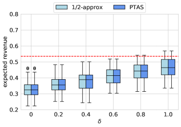
(a) The setting of high price sensitivity $(\beta=-1)$.

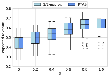
(b) The setting of low price sensitivity $(\beta=-0.1)$.

Figure 6: The boxplots of expected revenue obtained by our $1/2$-approx. algorithm and PTAS under different levels of fairness constraints (i.e., $\delta$). The boxplot extends from the first quartile to the third quartile, with a line at the median. The dashed line here shows the average optimal revenue in the absence of fairness constraints.

In terms of the number of sets we need to randomize over, what we observe in our synthetic experiments match our observations in Section 9. Figure 7 shows that in both settings with high and low price sensitivity, as $\delta$ increases, the average number of sets we need to randomize over decreases and the variance in the number of sets increases. This implies that there are more chances to consider a much smaller number of sets as fairness constraints relax.

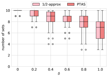
(a) The setting of high price sensitivity $(\beta=-1)$.

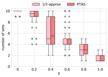
(b) The setting of low price sensitivity $(\beta=-0.1)$.

Figure 7: The boxplots of the number of randomized sets in the approximate solutions generated by our $1/2$-approx. algorithm and PTAS, under different levels of fairness constraints (i.e., $\delta$).

Comparison of $1/2$-Approx. Algorithm and PTAS. We note from Figures 6 and 7 that in both settings and under different levels of fairness constraints, the solutions returned by our $1/2$-approx. algorithm and PTAS are very close to each other, in terms of both the expected revenue and the number of randomized sets in the near-optimal solutions they produce. From Figure 7, it can be seen that both algorithms generate solutions that only involve a small number (at most $10$) assortments. This also matches what we observed in our case study in Section 9. In Table 2, we record the average runtime of the $1/2$-approx. algorithm and the PTAS on all of the synthetically generated instances. We observe that the $1/2$-approx. algorithm again demonstrates much faster computational performance than the PTAS, in terms of both the time taken by a single execution and the total time taken to solving Problem (fair). Note that the time taken to solve Problem (fair) by both algorithms gets longer for smaller $\delta$, which is because when the fairness constraint gets tighter, the feasibility region of Problem (fair) shrinks. Consequently, finding a near-optimal solution becomes more difficult, as at each iteration of the column generation method, the primal objective increases at a slower rate. Therefore, it usually takes more iterations for the column generation method to converge (i.e., when we no longer find a set that violates the dual fairness constraint of Problem (fair-dual) using our approximation algorithms). Nevertheless, under such a more difficult setting, the $1/2$-approx. algorithm still achieves much better runtime results. Given our observations in the synthetic experiments, we consider our $1/2$-approx. algorithm to be a viable practical option that not only produces near-optimal solutions far exceeding its theoretical guarantee, but also has fast computational performance.

Table 2: Average runtime comparison of $1/2$-approx. and PTAS algorithms in the synthetical experiments (the runtime is averaged across all instances with low/high price sensitivities).

	$\delta$	0	0.2	0.4	0.6	0.8	1.0
Time taken by a single execution (s)	$1/2$-approx	$2.9\times 10^{-1}$	$2.4\times 10^{-1}$	$1.9\times 10^{-1}$	$1.5\times 10^{-1}$	$1.1\times 10^{-1}$	$9.0\times 10^{-2}$
	PTAS	4.1	3.7	2.9	2.4	1.8	1.3
Total time taken in solving (fair) (s)	$1/2$-approx	7.1	5.6	4.0	2.8	2.1	1.5
	PTAS	98.0	83.5	58.9	41.8	31.0	21.6

17 Proof of Theorem 5.1

Here, we restate Problem (fair) for reader’s convenience.

$$\textsc{fair}~{}=~{}\max_{p(S):S\subseteq[n]} \sum_{S:|S|\leq K}p(S)\cdot\textsc{rev}(S)$$

s.t. $$\quad q_{j}\cdot\sum_{S:i\in S}O_{i}(S)p(S)-q_{i}\cdot\sum_{S:j\in S}O_{j}(S)p(S)\leq\delta\cdot q_{i}q_{j}\quad\quad~{}~{}~{}~{}~{}i,j\in[n],i\neq j$$

$$\sum_{S:|S|\leq K}p(S)\leq 1$$

$$\quad p(S)\geq 0\quad\quad\quad\quad\quad\quad\quad\quad\quad\quad\quad\quad\quad~{}~{}~{}~{}~{}~{}~{}~{}~{}~{}~{}~{}~{}~{}~{}~{}~{}~{}~{}S\subseteq[n],|S|\leq K\,,$$ (10)

We start by showing that Problem (fair) admits an optimal basic feasible solution (for definition of basic feasible solution, see Definition 2.9 in Bertsimas and Tsitsiklis [1997] or Section 24). Consider the polyhedron defined by the feasibility region of Problem (fair). Note that this polyhedron is (i) nonempty, because $p(S)=0$ for all $S\subseteq[n],|S|\leq K$ is a feasible solution for any $\delta\geq 0$; (ii) bounded, because $p(S)\in[0,1]$ for all $S\subseteq[n],|S|\leq K$. Then, by Theorem 2.6 in Bertsimas and Tsitsiklis [1997], there exists at least one extreme point in the polyhedron (for definition of extreme point, see Definition 2.6 in Bertsimas and Tsitsiklis [1997]). Since we have $\textsc{rev}(S)=\sum_{i\in S}\frac{r_{i}w_{i}}{1+w(S)}\leq\bar{r}$ for any $S$, this implies that $\sum_{S:|S|\leq K}p(S)\textsc{rev}(S)\leq\bar{r}$; that is, the objective of Problem (fair) is also bounded. By Theorem 2.8 in Bertsimas and Tsitsiklis [1997], since the polyhedron has at least one extreme point and Problem (fair) has a bounded optimal objective, there must exist one extreme point of the polyhedron that is optimal. By Theorem 2.3 in Bertsimas and Tsitsiklis [1997], we have that an extreme point is equivalent to a basic feasible solution. Hence, we must have a basic feasible solution to Problem (fair) that is optimal, which we denote by $p^{\star}(.)$.

Now, let $N=|\{S\subseteq[n]:|S|\leq K\}|$ be the number of variables in Problem (fair). There are $n(n-1)+1+N$ constraints in Problem (fair), where $n(n-1)$ of them are in the first set of constraints, and $N$ of them are the non-negativity constraints. By definition of a basic feasible solution, we must have that at least $N$ active (binding) constraints at $p^{\star}(.)$. That implies that at most $n(n-1)+1$ of the non-negativity constraints can be inactive, i.e. $p^{\star}(S)>0$. We have thus showed that $\big{|}\{S:p^{\star}(S)>0\}\big{|}\leq n(n-1)+1$. $\blacksquare$

18 Proof of Theorem 5.2

Revenue/marketshare-fair instance. Let us first consider the revenue/marketshare-fair instance, where $\Theta=(\mathbf{a},0,\mathbf{r},\mathbf{w},\mathbf{q})$. By Proposition 6.1, the StaticMNL algorithm introduced by Rusmevichientong et al. [2010] solves Problem (sub-dual($\mathbf{z},K$)) optimally and returns the optimal assortment $S^{\star}=\mathop{\rm arg\,max}_{S:|S|\leq K}~{}\textsc{rev-cost}(S,\mathbf{z})$. The StaticMNL algorithm leverages the structural properties of the MNL model to generate a sequence of $\mathcal{O}(n^{2})$ assortments that is guaranteed to include the optimal assortment. Hence, its running time is of order $\mathcal{O}(n^{2})$.

Visibility-fair and general instances. We now focus on visibility-fair and general instances, and establish the NP-completeness of Problem (sub-dual($\mathbf{z},K$)). We first show that Problem (sub-dual($\mathbf{z},K$)) is in NP. Then, we reduce an arbitrary instance of the partition problem, which is known to be NP-complete, to polynomially many visibility-fair instances of Problem (sub-dual($\mathbf{z},K$)).

To show that Problem (sub-dual($\mathbf{z},K$)) is in NP, note that the decision version of Problem (sub-dual($\mathbf{z},K$)) is: given a set $S$ and some value $\gamma$, we need to determine if $\textsc{rev-cost}(S,\mathbf{z})$ is greater than $\gamma$. We can compute $\textsc{rev-cost}(S,\mathbf{z})$ in polynomial time using Equation (3), since $\mathbf{z},\mathbf{r},\mathbf{w},\mathbf{q}$ are all known. This then allow us to tell if $\textsc{rev-cost}(S,\mathbf{z})>\gamma$ immediately. Hence, Problem (sub-dual($\mathbf{z},K$)) is in NP.

We will now show the NP-completeness of Problem (sub-dual($\mathbf{z},K$)) by considering an arbitrary instance of the partition problem, and solving it using polynomially many visibility-fair instances of Problem (sub-dual($\mathbf{z},K$)). The partition problem is known to be NP-complete [Hayes, 2002], and is stated as follows: given a set of $n$ positive integers $\{\alpha_{1},\alpha_{2},\dots,\alpha_{n}\}$, we would like to determine if there exists a subset $S\subset[n]$ such that $\sum_{i\in S}\alpha_{i}=\frac{1}{2}\sum_{i\in[n]}\alpha_{i}:=L$, and find the set $S$ if it exists.

Before proceeding, let us first define an auxiliary optimization problem that we will work with throughout the proof. For some given vector $\mathbf{c}^{\prime}$, we define Problem (sub-dual-aux($\mathbf{c}^{\prime},K$)) as:

$$\textsc{sub-dual-aux}(\mathbf{c}^{\prime},K)=\max_{S:|S|\leq K}\frac{\sum_{i\in S}w_{i}}{1+\sum_{i\in S}w_{i}}-\sum_{i\in S}c^{\prime}_{i}\,. \mathbf{c}^{\prime},K$$ (sub-dual-aux())

We denote the objective function of Problem (sub-dual-aux($\mathbf{c}^{\prime},K$)) as

$$\textsc{rev-cost-aux}(S,\mathbf{c}^{\prime}):=\frac{\sum_{i\in S}w_{i}}{1+\sum_{i\in S}w_{i}}-\sum_{i\in S}c^{\prime}_{i}\,.$$

Our proof of Theorem 5.2 consists of two parts. In Part 1, we reduce an arbitrary instance of the partition problem to a particular instance of Problem (sub-dual-aux($\mathbf{c}^{\prime},K$)). In Part 2, we show that this instance of Problem (sub-dual-aux($\mathbf{c}^{\prime},K$)) can be further reduced to a polynomial number of visibility-fair instances of Problem (sub-dual($\mathbf{z},K$)).

Part 1. Let $\{\alpha_{1},\alpha_{2},\dots,\alpha_{n}\}$ be an instance of the partition problem. We first reduce it to the auxiliary optimization problem by creating an instance of Problem (sub-dual-aux($\mathbf{c}^{\prime},K$)) as follows. For each $i\in[n]$, let $w_{i}=\alpha_{i}/L$ and $c^{\prime}_{i}=\alpha_{i}/4L$. Let $K=n/2$. Additionally, let $A(S):=\sum_{i\in S}\alpha_{i}$. We can rewrite the objective function of Problem (sub-dual-aux($\mathbf{c}^{\prime},K$)) to be a function dependent on $A(S)$:

$$\frac{\sum_{i\in S}w_{i}}{1+\sum_{i\in S}w_{i}}-\sum_{i\in S}c^{\prime}_{i}=\frac{A(S)}{L+A(S)}-\frac{A(S)}{4L}=\frac{3LA(S)-(A(S))^{2}}{4L^{2}+4LA(S)}:=f(A(S)),$$

where we let $f(x)=\dfrac{3Lx-x^{2}}{4L^{2}+4Lx}$ for $x\geq 0$. Differentiating $f(x)$ with respect to $x$ gives

$$f^{\prime}(x)=\frac{-x^{2}-2Lx+3L^{2}}{4L(L+x)^{2}}\,.$$

Taking $f^{\prime}(x)=0$ gives $x=L$. Since $f^{\prime}(x)<0$ for $x>L$ and $f^{\prime}(x)>0$ for $0\leq x<L$, we have that for $x\geq 0$, $f(x)$ is uniquely maximized at $x=L$ and $\max_{x\geq 0}f(x)=f(L)=\frac{1}{4}$.

We now show that we can determine whether a partition $S$ exists and, if it exists, find $S$ if and only if we can find the optimal set $S^{\star}$ for instance of Problem (sub-dual-aux($\mathbf{c}^{\prime},K$)) and it attains optimal objective value of $1/4$. Suppose a partition $S^{\star}$ exists such that $A(S^{\star})=\sum_{i\in S^{\star}}a_{i}=L$, we have

$$\frac{1}{4}\geq\textsc{sub-dual-aux}(\mathbf{c}^{\prime},K)=\max_{{S\subset[n]}\atop{|S|\leq K}}f(A(S))\geq f(A(S^{\star}))=f(L)=\frac{1}{4}.$$

Hence, the inequalities above should be equalities. We have that $S^{\star}$ is the optimal set for Problem (sub-dual-aux($\mathbf{c}^{\prime},K$)) and the optimal objective value is $f(A(S^{\star}))=1/4$. Reversely, if we find $S^{\star}=\mathop{\rm arg\,max}_{{S\subset[n]}\atop{|S|\leq K}}f(A(S))$ and $\max_{{S\subset[n]}\atop{|S|\leq K}}f(A(S))=f(L)=\frac{1}{4}$, we must have that $A(S^{\star})=\sum_{i\in S^{\star}}\alpha_{i}=L$, and $S^{\star}$ is thus a solution to the partition problem. The discussion above shows that we can reduce the partition problem to the instance of Problem (sub-dual-aux($\mathbf{c}^{\prime},K$)).

Part 2. Now, it suffices to show that the instance of Problem (sub-dual-aux($\mathbf{c}^{\prime},K$)) defined above can be solved using polynomially many instances of Problem (sub-dual($\mathbf{z},K$)). In particular, here we consider visibility-fair instances of Problem (sub-dual($\mathbf{z},K$)) where $a_{i}=0$ and $b_{i}=1$ for all $i\in[n]$. We would also let all items have unit revenue, i.e., $r_{i}=1$ for all $i\in[n]$. Such visibility-fair instances of Problem (sub-dual($\mathbf{z},K$)) takes the following form:

$$\textsc{sub-dual}(\mathbf{z},K)=\max_{S:|S|\leq K}~{}\frac{\sum_{i\in S}w_{i}}{1+\sum_{i\in S}w_{i}}-\sum_{i\in S}c_{i}(\mathbf{z})=\max_{S:|S|\leq K}~{}\textsc{rev-cost}(S,\mathbf{z})\,,$$ (11)

where post-fairness revenue of item $i$ is $\mathcal{r}_{i}(\mathbf{z})=1$, post-fairness cost of item $i$ is $\mathfrak{c}_{i}(\mathbf{z})=c_{i}(\mathbf{z})$, and cost $c_{i}(\mathbf{z})$ is defined in Equation (6). Note that Problem (sub-dual-aux($\mathbf{c}^{\prime},K$)) only differs from such visibility-fair instance of Problem (sub-dual($\mathbf{z},K$)) in the second term of the objective function, where $\mathbf{c}^{\prime}$ can be any vector and does not depend on $\mathbf{z}$.

Without loss of generality, assume that $\alpha_{1}\geq\alpha_{2}\geq\dots\geq\alpha_{n}$. Before proceeding, let us first make the following definitions.

1. For every $k\in[n]$, let $(\textsc{sub-dual-aux}^{(k)})$ denote an instance of Problem (sub-dual-aux($\mathbf{c}^{\prime},K$)) with $k$ items, where $\mathbf{w}=(w_{1},\dots,w_{k})=(\alpha_{1}/L,\dots,\alpha_{k}/L)$, $\mathbf{c}^{\prime}=(c^{\prime}_{1},\dots,c^{\prime}_{k})=(\alpha_{1}/4L,\dots,\alpha_{k}/L)$ and $K=n/2$. The instance of Problem (sub-dual-aux($\mathbf{c}^{\prime},K$)) that we considered in Part 1 of the proof is $(\textsc{sub-dual-aux}^{(n)})$.

2. For every $k\in[n]$, let $(\textsc{sub-dual}^{(k)})$ denote a visibility-fair instance of Problem (sub-dual($\mathbf{z},K$)) with $k$ items, where $\mathbf{a}=\mathbf{0},\mathbf{b}=\mathbf{1}=(1,\dots,1),\mathbf{r}=\mathbf{1}=(1,\dots,1),\mathbf{w}=(w_{1},\dots,w_{k})=(\alpha_{1}/L,\dots,\alpha_{k}/L),\mathbf{q}=\mathbf{w}$, and $K=n/2$. We choose $\mathbf{z}=\mathbf{z}^{(k)}$ such that $c_{i}(\mathbf{z}^{(k)})=c^{\prime}_{i}=\alpha_{i}/4L$ for $i\in[k-1]$. Note that such $\mathbf{z}^{(k)}$ always exists, since the linear system

   $$c_{i}(\mathbf{z}^{(k)})=\sum_{j\neq i}(z^{(k)}_{ij}-z^{(k)}_{ji})q_{j}=\sum_{j\neq i}(z^{(k)}_{ij}-z^{(k)}_{ji})w_{j}=\frac{\alpha_{i}}{4L},\quad\forall i\in[k-1]$$

   can be written as

   $$\sum_{j\neq i}\mathbbm{1}_{\{i<j\}}\frac{\alpha_{j}}{L}x_{ij}=\frac{\alpha_{i}}{4L},\quad\forall i\in[k-1]$$

   where $x_{ij}=z^{(k)}_{ij}-z^{(k)}_{ji}$ for all $i<j$. The rows of this $(k-1)\times(k-1)(k-2)$ linear system are linearly independent, and hence there exists a feasible solution. However, via row operations, one can check that the values of $c_{1}(\mathbf{z}^{(k)}),\dots,c_{k-1}(\mathbf{z}^{(k)})$ uniquely determine the value of $c_{k}(\mathbf{z}^{(k)})$ to be

   $$c_{k}(\mathbf{z}^{(k)})=-\frac{\sum_{i<k}\alpha_{i}^{2}}{4L\alpha_{k}}.$$

Note that the only difference between the instance $(\textsc{sub-dual}^{(k)})$ and $(\textsc{sub-dual-aux}^{(k)})$ is in the difference between $c_{k}(\mathbf{z}^{(k)})$ and $c_{k}^{\prime}$. Additionally, we have $c_{k}(\mathbf{z}^{(k)})=-(\sum_{i<k}\alpha_{i}^{2})/(4L\alpha_{k})\leq\alpha_{k}/4L=c_{k}^{\prime}$ because $\alpha_{i}$’s are all positive integers.

Having defined the two types of instances, our proof of Part 2 proceeds in three steps: (i) first, we establish an important relationship between the two functions rev-cost and rev-cost-aux; (ii) next, we show that for any $k\in[n]$, we can solve the instance $(\textsc{sub-dual-aux}^{(k)})$ if we can solve $(\textsc{sub-dual}^{(k)})$ and $(\textsc{sub-dual-aux}^{(k-1)})$; (iii) based on that, we use a recursive approach to show that the instance $(\textsc{sub-dual-aux}^{(n)})$ considered in Part 1 of the proof can be solved as long as we can solve $(\textsc{sub-dual}^{(n)}),\dots,(\textsc{sub-dual}^{(2)})$, which are $n-1$ instances of Problem (sub-dual($\mathbf{z},K$)).

Step 1. Fix $k\in[n]$. Let us start by considering the two instances $(\textsc{sub-dual}^{(k)})$ and $(\textsc{sub-dual-aux}^{(k)})$. Recall that the objective function of $(\textsc{sub-dual}^{(k)})$ is:

$$\textsc{rev-cost}(S,\mathbf{z}^{(k)})=\frac{\sum_{i\in S}w_{i}}{1+\sum_{i\in S}w_{i}}-\sum_{i\in S}c_{i}(\mathbf{z}^{(k)})$$

and the objective function of $(\textsc{sub-dual-aux}^{(k)})$ is

$$\textsc{rev-cost-aux}(S,\mathbf{c})=\frac{\sum_{i\in S}w_{i}}{1+\sum_{i\in S}w_{i}}-\sum_{i\in S}c^{\prime}_{i}\,.$$

Since $c_{i}(\mathbf{z}^{(k)})=c^{\prime}_{i}$ for all $i\in[k-1]$, we must have the following:

• For any set $S$ such that $k\notin S$, we must have $\textsc{rev-cost}(S,\mathbf{z}^{(k)})=\textsc{rev-cost-aux}(S,\mathbf{c}^{\prime})$.

• For any set $S$ such that $k\in S$, we must have

  $$\textsc{rev-cost}(S,\mathbf{z}^{(k)})=\textsc{rev-cost-aux}(S,\mathbf{c}^{\prime})+\frac{\alpha_{k}}{4L}+\frac{\sum_{i<k}\alpha_{i}^{2}}{4L\alpha_{k}}\geq\textsc{rev-cost-aux}(S,\mathbf{c}^{\prime}).$$

Step 2. Now, suppose that we have solved $(\textsc{sub-dual}^{(k)})$ with $S^{\star}_{k}$ as its optimal solution, and we have also solved $(\textsc{sub-dual-aux}^{(k-1)})$ with $S^{\prime}_{k-1}$ as its optimal solution. We claim that the optimal solution to $(\textsc{sub-dual-aux}^{(k)})$, $S^{\prime}_{k}$, would then be the best set among $S^{\star}_{k}$ and $S^{\prime}_{k-1}$.

To see why, we divide our arguments into the following cases:

• Case 1: $k\notin S^{\star}_{k}$. In this case, we claim that $S^{\star}_{k}$ is an optimal solution to $(\textsc{sub-dual-aux}^{(k)})$. Let $S^{\prime}\in[k],|S^{\prime}|\leq K$ be any set that is different from $S^{\star}_{k}$. There are again two possibilities:

  • If $k\notin S^{\prime}$, we have

    $$\textsc{rev-cost-aux}(S^{\prime},\mathbf{c}^{\prime})=\textsc{rev-cost}(S^{\prime},\mathbf{z}^{(k)})\leq\textsc{rev-cost}(S^{\star}_{k},\mathbf{z}^{(k)})=\textsc{rev-cost-aux}(S^{\star}_{k},\mathbf{c}^{\prime})\,,$$

    where the two equalities follow from Step 1.

  • If $k\in S^{\prime}$, we have

    $$\textsc{rev-cost-aux}(S^{\prime},\mathbf{c}^{\prime})\leq\textsc{rev-cost}(S^{\prime},\mathbf{z}^{(k)})\leq\textsc{rev-cost}(S^{\star}_{k},\mathbf{z}^{(k)})=\textsc{rev-cost-aux}(S^{\star}_{k},\mathbf{c}^{\prime})\,,$$

    where the first inequality and the last equality follow from Step 1.

  Since we have $\textsc{rev-cost-aux}(S^{\prime},\mathbf{c}^{\prime})\leq\textsc{rev-cost-aux}(S^{\star}_{k},\mathbf{c})$ for any set $S^{\prime}$, $S^{\star}_{k}$ must be an optimal solution to $(\textsc{sub-dual-aux}^{(k)})$.

• Case 2: $k\in S^{\star}_{k}$. In this case, we claim that the optimal solution to $(\textsc{sub-dual-aux}^{(k)})$, which we denote by $S^{\prime}_{k}$, is either $S^{\star}_{k}$ or $S^{\prime}_{k-1}$. Let us again consider the two possibilities:

  • If $k\in S^{\prime}_{k}$, we must have

    $$\textsc{rev-cost-aux}(S^{\prime}_{k},\mathbf{c}^{\prime}) =\textsc{rev-cost}(S^{\prime}_{k},\mathbf{z}^{(k)})-\big{(}\frac{\alpha_{k}}{4L}+\frac{\sum_{i<k}\alpha_{i}^{2}}{4L\alpha_{k}}\big{)}$$

    $$\leq\textsc{rev-cost}(S^{\star}_{k},\mathbf{z}^{(k)})-\big{(}\frac{\alpha_{k}}{4L}+\frac{\sum_{i<k}\alpha_{i}^{2}}{4L\alpha_{k}}\big{)}$$

    $$=\textsc{rev-cost-aux}(S^{\star}_{k},\mathbf{c}^{\prime}).$$

  where the equalities follow from Step 1. Hence, in this case, $S^{\star}_{k}$ is an optimal solution to $(\textsc{sub-dual-aux}^{(k)})$.

• If $k\notin S^{\prime}_{k}$. In this case, an optimal solution to $(\textsc{sub-dual-aux}^{(k)})$ is simply the optimal solution to $(\textsc{sub-dual-aux}^{(k-1)})$; that is, $S^{\prime}_{k-1}$.

To summarize, our case discussion above shows that to solve $(\textsc{sub-dual-aux}^{(k)})$, it suffices to solve $(\textsc{sub-dual}^{(k)})$ and $(\textsc{sub-dual-aux}^{(k-1)})$.

Step 3. Finally, we consider the instance $(\textsc{sub-dual-aux}^{(n)})$ from Part 1 of the proof. Since we have shown in Step 2 that for any $k\in[n]$, we can solve $(\textsc{sub-dual-aux}^{(k)})$ as long as we can solve $(\textsc{sub-dual}^{(k)})$ and $(\textsc{sub-dual-aux}^{(k-1)})$, we can solve $(\textsc{sub-dual-aux}^{(n)})$ in a recursive manner. This requires us to solve at most $n-1$ visibility-fair instances of Problem (sub-dual($\mathbf{z},K$)), i.e., $(\textsc{sub-dual}^{(n)}),(\textsc{sub-dual}^{(n-1)}),\dots,(\textsc{sub-dual}^{(2)})$ and one instance of Problem (sub-dual-aux($\mathbf{c}^{\prime},K$)), i.e., $(\textsc{sub-dual-aux}^{(1)})$, for which the solution is trivial to obtain.

In summary, in Part 2 we have shown that $(\textsc{sub-dual-aux}^{(n)})$ can be solved using a polynomial number of visibility-fair instances of Problem (sub-dual($\mathbf{z},K$)). Together, Part 1 and 2 of the proof show that an arbitrary instance of the partition problem can be solved using polynomially many visibility-fair instances of Problem (sub-dual($\mathbf{z},K$)). This establishes the NP-completeness of Problem (sub-dual($\mathbf{z},K$)). In particular, since we only consider visibility-fair instances of Problem (sub-dual($\mathbf{z},K$)) with uniform revenues (i.e., $r_{i}=1$ for all $i\in[n]$), our proof above in fact shows that even for visibility-fair instances with uniform revenues, Problem (sub-dual($\mathbf{z},K$)) is also NP-complete. $\blacksquare$

19 Proof of Theorem 5.3

Our proof of Theorem 5.3 consists of two segments. In Segment 1, we show that our fair Ellipsoid-based algorithm gives a $\beta$-approximate solution for Problem (fair), and the returned solution requires us to randomize over a polynomial number of sets. In Segment 2, we show that the runtime of our fair Ellipsoid-based algorithm is polynomial in the size of our input.

Segment 1. Before proceeding, recall that in Section 5.3, we define $\mathcal{V}=\{S:|S|\leq K\}$ as the collection of sets that violate the dual fairness constraint. The first segment of our proof consists of three parts: (i) We first show that if we apply the Ellipsoid method equipped with a $\beta$-approximate separation oracle to the dual problem (fair-dual), we will end up with a dual objective $r^{\prime}$ that is not too far away from the optimal primal objective fair. That is, it satisfies $r^{\prime}\geq\beta\cdot\ref{eq:problem:fair}$. (ii) We then construct a auxiliary dual problem (fair-dual-aux), in which we only keep the dual fairness constraints for $S\in\mathcal{V}$; and the corresponding auxiliary primal problem (fair-aux), in which we enforce $p(S)=0$ for all $S\notin\mathcal{V}$. The auxiliary primal problem is the one we solve in Step 2 of our algorithm. We will show that the optimal objectives of both Problem (fair-dual-aux) and (fair-aux) exceeds $r^{\prime}$, and hence exceeds $\beta\cdot\ref{eq:problem:fair}$. (iii) Finally, we show that the number of sets in $\mathcal{V}$ is polynomial, which implies that $|\{S:\widehat{p}(S)>0\}|$ is polynomial.

Part 1. As described in Step 1 of the fair Ellipsoid-based algorithm, suppose that we apply the Ellipsoid method to the dual problem (fair-dual), and use algorithm $\mathcal{A}$ as the $\beta$-approximate separation oracle. Let $(\mathbf{z}^{\prime},\rho^{\prime})$ be the solution we get at the end of the Ellipsoid method, and let $r^{\prime}=\rho^{\prime}+\sum_{i=1}^{n}\sum_{j=1,j\neq i}^{n}\delta\cdot{q}_{i}q_{j}\cdot z^{\prime}_{ij}$ denote its dual objective. We first note that the solution $(\mathbf{z}^{\prime},\rho^{\prime})$ is not necessarily feasible for Problem (fair-dual). This is because when we examine the feasibility of this solution, our separation oracle first solves Problem $(\textsc{sub-dual}(\mathbf{z}^{\prime},K))$, and obtained a set $S_{\mathcal{A}}$ such that $\textsc{rev-cost}(S_{\mathcal{A}},\mathbf{z}^{\prime})\geq\beta\cdot\textsc{sub-dual}(\mathbf{z}^{\prime},K)$. The Ellipsoid method has declared solution $(\mathbf{z}^{\prime},\rho^{\prime})$ feasible because $\textsc{rev-cost}(S_{\mathcal{A}},\mathbf{z}^{\prime})\leq\rho^{\prime}$. However, it is still possible that $\textsc{sub-dual}(\mathbf{z}^{\prime},K)=\max_{|S|\leq K}\textsc{rev-cost}(S,\mathbf{z}^{\prime})>\rho^{\prime}$. We will first show that the dual objective that we obtain here would still be close to the optimal primal objective fair.

Suppose that we solve the dual problem (fair-dual) by additionally fixing $\mathbf{z}=\mathbf{z}^{\prime}$. This problem has a trivial solution because $\rho$ is the only decision variable, and it must be chosen such that the inequality in Equation (4) is tight. That is, we set $\rho=\textsc{sub-dual}(\mathbf{z}^{\prime},K)$ and the optimal objective is

$$r_{\mathbf{z^{\prime}}}:=\textsc{sub-dual}(\mathbf{z}^{\prime},K)+\sum_{i=1}^{n}\sum_{j=1,j\neq i}^{n}\delta\cdot{q}_{i}q_{j}\cdot z^{\prime}_{ij}$$

Clearly, we must have $\ref{eq:problem:dual}\leq r_{\mathbf{z^{\prime}}}$ since fixing $\mathbf{z}=\mathbf{z^{\prime}}$ is equivalent to introducing more constraints into Problem (fair-dual). Note that we also have

$$r^{\prime}=\rho^{\prime}+\sum_{i=1}^{n}\sum_{j=1,j\neq i}^{n}\delta\cdot{q}_{i}q_{j}\cdot z^{\prime}_{ij}\geq\beta\cdot\textsc{sub-dual}(\mathbf{z}^{\prime},K)+\beta\cdot\sum_{i=1}^{n}\sum_{j=1,j\neq i}^{n}\delta\cdot{q}_{i}q_{j}\cdot z^{\prime}_{ij}=\beta\cdot r_{\mathbf{z^{\prime}}}\,,$$

where the inequality follows from $\rho^{\prime}\geq\textsc{rev-cost}(S_{\mathcal{A}},\mathbf{z}^{\prime})\geq\beta\cdot\textsc{sub-dual}(\mathbf{z}^{\prime},K)$ and $z^{\prime}_{ij}\geq 0$. Together, the two inequalities above give

$$r^{\prime}\geq\beta\cdot r_{\mathbf{z^{\prime}}}\geq\beta\cdot\ref{eq:problem:dual}=\beta\cdot\ref{eq:problem:fair}\,,$$ (12)

where the last equality follows from strong duality. The inequality in Equation (12) is a key inequality that we will continue to work with in Part 2.

Part 2. In Part 2, we first create an auxiliary version of the dual problem, defined as follows:

$$\begin{aligned} \textsc{fair-dual-aux}~{}=~{}\min_{\rho\geq 0,\mathbf{z}\geq\mathbf{0}}~{}~{}&\,\rho+\sum_{i=1}^{n}\sum_{j=1,j\neq i}^{n}\delta\cdot{q}_{i}q_{j}\cdot z_{ij}\\ \text{ s.t. }&\sum_{i\in S}O_{i}(S)\cdot\left(\sum_{j=1,j\neq i}^{n}(z_{ij}-z_{ji}){q}_{j}\right)+\rho\geq\textsc{rev}(S),\quad&\forall S\in\mathcal{V}\end{aligned}$$ (fair-dual-aux)

Note that the auxiliary dual problem is different from Problem (fair-dual), because in the auxiliary dual problem, we only enforces the constraints on sets $S\in\mathcal{V}$, where $\mathcal{V}$ is the collection sets for which the dual fairness constraint has been violated when we solve Problem (fair-dual). Since the unviolated constraints did not impact any of the iteration in the Ellipsoid method when we solve Problem (fair-dual), if we now apply the Ellipsoid method with the $\beta$-approximate separation oracle to solve Problem (fair-dual-aux), the solution we obtain would still be $(\mathbf{z}^{\prime},\rho^{\prime})$, which gives objective value $r^{\prime}$.

Similar to our arguments in Part 1, we note that when we apply the Ellipsoid method using our approximate separation oracle, we essentially increases the feasibility region of the linear program. Hence, the solution $(\mathbf{z}^{\prime},\rho^{\prime})$ we found at the end of the Ellipsoid method might not be feasible and the objective we obtain is less than or equal to the actual optimal objective. That is, we must have $r^{\prime}\leq\ref{eq:problem:dual-aux}$. This, along with the inequality we established in Equation (12), gives

$$\ref{eq:problem:dual-aux}\geq r^{\prime}\geq\beta\cdot\ref{eq:problem:fair}\,.$$

Consider the primal counterpart to the auxiliary dual problem (fair-dual-aux) defined below:

$$\textsc{fair-aux}~{}=~{}\max_{p(S)\geq 0:S\in\mathcal{V}} \sum_{S:S\in\mathcal{V}}p(S)\cdot\textsc{rev}(S)$$

s.t. $$\quad q_{j}\cdot\sum_{S:i\in S}O_{i}(S)p(S)-q_{i}\cdot\sum_{S:j\in S}O_{j}(S)p(S)\leq\delta\quad\quad~{}~{}~{}~{}~{}i,j\in[n]$$

$$\sum_{S:|S|\in\mathcal{V}}p(S)\leq 1$$ (fair-aux)

Essentially, this differs from Problem (fair) in that here, we set $p(S)=0$ for all $S\notin\mathcal{V}$. This is the primal problem that we solve in Step 2 of the fair Ellipsoid-based algorithm. Let $\widehat{p}(S)$ denote the optimal solution to Problem (fair-aux). By the strong duality theorem , we have $\ref{eq:problem:fair-aux}=\ref{eq:problem:dual-aux}\geq\beta\cdot\ref{eq:problem:fair}$. We have thereby showed that our algorithm returns a solution $\widehat{p}(S)$ that is an $\beta$-approximate feasible solution to Problem (fair).

Part 3. Since we have $\widehat{p}(S)=0$ for all $S\notin\mathcal{V}$, the number of sets that we need to randomize over, i.e. $|\{S:\widehat{p}(S)>0\}|$, is bounded by $|\mathcal{V}|$. Recall that in the dual problem (fair-dual), we have $\mathcal{O}(n^{2})$ variables. By Bertsimas and Tsitsiklis [1997], given a separation oracle, the Ellipsoid method would solve (fair-dual) in at most $\mathcal{O}(n^{12}\log(nq_{\max}))$ iterations. Within each iteration, one violated constraint is identified. Hence, we must have that $|\mathcal{V}|$, i.e., the number of sets for which the dual fairness constraints in (fair-dual) is violated, is polynomial in $n$ and $\log(q_{\max})$. This thus proves that $|\{S:\widehat{p}(S)>0\}|$ is polynomial in the size of our input.

Segment 2. In the second segment of the proof, we remark on the runtime of our fair Ellipsoid-based algorithm. In Step 1 of the algorithm, the Ellipsoid method equipped with a polynomial-time separating oracle runs in polynomial time. In Step 2 of the algorithm, solving a linear program with polynomial number of variables also takes polynomial time. Hence, given a polynomial-time separation oracle, the total time taken by the fair Ellipsoid-based algorithm is polynomial in the size of our input. $\blacksquare$

20 Proof of Theorem 6.2

Let $S^{\star}\in\arg\max_{S:|S|\leq K}\textsc{rev-cost}(S,\mathbf{z})$ and let $W^{\star}=\sum_{i\in S^{\star}}w_{i}$. We must have

$$\textsc{sub-dual}(\mathbf{z},K)=\textsc{rev-cost}(S^{\star},\mathbf{z})\leq\textsc{kp}(W^{\star},K)\leq\max_{W\geq 0}~{}\textsc{kp}(W,K)\,.$$ (13)

The first inequality follows from the fact that (i) $S^{\star}$ is a feasible solution to Problem $\textsc{kp}(W^{\star},K)$ since $|S^{\star}|\leq K$ and $\sum_{i\in S^{\star}}w_{i}=W^{\star}$ by definition, and (ii)

$$\textsc{rev-cost}(S^{\star},\mathbf{z})=\frac{\sum_{i\in S^{\star}}\mathcal{r}_{i}w_{i}}{1+\sum_{i\in S^{\star}}w_{i}}-\sum_{i\in S^{\star}}\mathfrak{c}_{i}=\sum_{i\in S^{\star}}\left(\frac{\mathcal{r}_{i}w_{i}}{1+W^{\star}}-\mathfrak{c}_{i}\right),$$

where the right-hand side (i.e., $\sum_{i\in S^{\star}}(\frac{\mathcal{r}_{i}w_{i}}{1+W^{\star}}-\mathfrak{c}_{i})$) is the objective value of the knapsack problem $(\textsc{kp}(W^{\star},K))$ at set $S^{\star}$, which is clearly upper bounded by its optimal objective value $\textsc{kp}(W^{\star},K)$.

Conversely, let $\max_{W\geq 0}\textsc{kp}(W,K)$ be obtained at capacity $\widetilde{W}$ and with optimal set $\widetilde{S}$, i.e., $\widetilde{S}$ is the optimal solution to Problem $\textsc{kp}(\widetilde{W},K)$. We then have

$$\max_{W\geq 0}\textsc{kp}(W,K)=\textsc{kp}(\widetilde{W},K) =\sum_{i\in\widetilde{S}}\left[\frac{\mathcal{r}_{i}w_{i}}{1+\widetilde{W}}-\mathfrak{c}_{i}\right]$$ (14)

$$\leq\sum_{i\in\widetilde{S}}\frac{\mathcal{r}_{i}w_{i}}{1+\sum_{i\in\widetilde{S}}w_{i}}-\sum_{i\in\widetilde{S}}\mathfrak{c}_{i}=\textsc{rev-cost}(\widetilde{S},\mathbf{z})\leq\max_{|S|\leq K}\textsc{rev-cost}(S,\mathbf{z})\,,$$

where the first inequality follows from the feasibility of $\widetilde{S}$ for Problem $\textsc{kp}(\widetilde{W},K)$, which implies that $\sum_{i\in\widetilde{S}}w_{i}\leq\widetilde{W}$, and the second inequality follows from $|\widetilde{S}|\leq K$.

Overall, Equations (13) and (14) together imply that $\textsc{sub-dual}(\mathbf{z},K)=\max_{S:|S|\leq K}\textsc{rev-cost}(S,\mathbf{z})=\max_{W\geq 0}\textsc{kp}(W,K),$ as desired. $\blacksquare$

21 Proof of Theorem 7.3

The proof consists of two segments. In the first segment, we show that if Algorithm 1 returns collection $\mathcal{C}_{I}$ and set $S_{I}$, we would have that for any $W\in I$, there exists a set $S_{W}\in\mathcal{C}_{I}$ such that

$$\textsc{rev-cost}(S_{W},\mathbf{z})\geq\frac{1}{2}\textsc{kp}(W,K)\,,$$

which then implies

$$\textsc{rev-cost}(S_{I},\mathbf{z})\geq\frac{1}{2}\max_{W\in I}~{}\textsc{kp}(W,K)\,.$$

In the second segment, we bound the runtime of the algorithm.

Segment 1. We start by considering the LP relaxation of the original knapsack problem, i.e., Problem ($\textsc{kp-relax}(W,K)$), and making the following claim:

Claim 1

For any $W\in I$, in the collection of assortments $\mathcal{C}_{I}$ returned by Algorithm 1, there exists an assortment $S_{W}$ such that $S_{W}$ is an integer $1/2$-approx. feasible solution for Problem $\textsc{kp-relax}(W,K)$.

Given that Claim 1 holds, we then have

$$\textsc{rev-cost}(S_{W},\mathbf{z})=\sum_{i\in S_{W}}\big{(}\frac{\mathcal{r}_{i}w_{i}}{1+\sum_{i\in S_{W}}w_{i}}-\mathfrak{c}_{i}\big{)}\geq\sum_{i\in S_{W}}\big{(}\frac{\mathcal{r}_{i}w_{i}}{1+W}-\mathfrak{c}_{i}\big{)}\geq\frac{1}{2}\textsc{kp-relax}(W,K)\geq\frac{1}{2}\textsc{kp}(W,K),$$ (15)

where the first inequality follows from the feasibility of $S_{W}$ (i.e., $\sum_{i\in S_{W}}w_{i}\leq W$); the second inequality follows from Claim 1; and the third inequality follows from $\textsc{kp-relax}(W,K)$ being an upper bound of $\textsc{kp}(W,K)$. Let $W^{\star}=\mathop{\rm arg\,max}_{W\in I}\textsc{kp}(W,K)$. This then further gives

$$\textsc{rev-cost}(S_{I},\mathbf{z})\geq\textsc{rev-cost}(S_{W^{\star}},\mathbf{z})\geq\frac{1}{2}\textsc{kp}(W^{\star},K)=\frac{1}{2}\max_{W\in I}~{}\textsc{kp}(W,K)\,,$$ (16)

where the first inequality follows from $S_{I}=\arg\max_{S\in\mathcal{C}_{I}}\textsc{rev-cost}(S,\mathbf{z})$ (Step 4 of Algorithm 1) and that $S_{W^{\star}}\in\mathcal{C}_{I}$; and the second inequality follows from Equation (15). This thus proves the statement of Theorem 7.3.

In the following, we provide a proof for Claim 1. Our proof consists of five parts. In Part 1, we first consider the capacity level $W_{\text{binding}}$, which is the maximum capacity level under which the capacity constraint is binding for the relaxed knapsack problems on $I$. We show that it suffices to show Claim 1 for $W<W_{\text{binding}}$. This then allows us to justify the stopping rules in Step 2b and Step 3(b)iii of the algorithm; see Parts 2 and 3 of the proof. Recall that in Algorithm 1, we consider the two intervals $I_{\text{low}}=I\cap[0,W_{\textsc{TH}})$ and $I_{\text{high}}=I\cap[W_{\textsc{TH}},\infty)$ separately. In Part 2, we show that when we hit the stopping rule in Step 2b, we have reached the upper bound $W_{\text{binding}}$ and there is no need to consider the interval $I_{\text{high}}$. Similarly, in Part 3, we show that when we hit stopping rule in Step 3(b)iii, we have reached $W_{\text{binding}}$ and there is no need to consider larger $W$’s. In Part 4 of the proof, we show that if $W\in I_{\text{low}}$, there exists a $1/2$-approx. solution $S_{W}\in\mathcal{C}_{I}$. In Part 5, which is one of the most challenging parts of the proof, using induction, we show that if $W\in I_{\text{high}}$, there exists a $1/2$-approx. solution $S_{W}\in\mathcal{C}_{I}$.

Part 1: we only need to show Claim 1 for $W\leq W_{\text{binding}}$. Let $W_{\text{binding}}$ be the maximum capacity level $W\in I$ for which the capacity constraint is binding for Problem ($\textsc{kp-relax}(W,K)$), i.e.,

$$W_{\text{binding}}:=\sup\Big{\{}W\in I:\sum_{i\in[n]}w_{i}x_{i}^{\star}(W)=W\Big{\}}~{}\text{and}~{}\sum_{i\in[n]}w_{i}x_{i}^{\star}(W^{\prime})<W^{\prime}~{}~{}\forall~{}W^{\prime}\in I\cap(W_{\text{binding}},\infty)\,.$$ (17)

If the capacity constraint is binding for all $W\in I$, we let $W_{\text{binding}}=W_{\max}$; if the capacity constraint is non-binding for all $W\in I$, we let $W_{\text{binding}}=W_{\min}$. Lemma 21.1 shows that $W_{\text{binding}}$ is well-defined. The lemma states that if the capacity constraint is non-binding at some capacity level $\widetilde{W}$, Problem ($\textsc{kp-relax}(W,K)$) will have a non-binding capacity constraint for all $W>\widetilde{W}$.

Lemma 21.1

Consider a capacity level $\widetilde{W}>0$, and suppose that the capacity constraint is non-binding at the optimal basic solution $\mathbf{x}^{\star}(\widetilde{W})$ to $\textsc{kp-relax}(\widetilde{W},K)$. That is, $\sum_{i\in[n]}w_{i}x^{\star}_{i}(\widetilde{W})<\widetilde{W}$. Then, for any $W>\widetilde{W}$ such that $W\in I$, we have $\sum_{i\in[n]}w_{i}x_{i}^{\star}(W)<W$.

We now note that if $W>W_{\text{binding}}$, then we must have

$$\textsc{kp}(W_{\text{binding}},K)>\textsc{kp}(W,K)\,.$$

To see why, we first assume, without loss of generality, that on the well-behaving interval $I$, the items are ranked by the order of their utilities, i.e., $u_{1}(W)\geq u_{2}(W)\geq\dots\geq u_{n}(W)$. Then, if there exists $W\in I$ such that $W>W_{\text{binding}}$, we must have that $W_{\text{binding}}\geq\sum_{i\in[K]}w_{i}$. That is, the $K$ items with the top utilities can fit into the knapsack of size $W_{\text{binding}}$. Since the ordering of utilities of items do not change on $I$, we then have

$$\textsc{kp}(W_{\text{binding}},K)=\sum_{i\in[k]}u_{i}(W_{\text{binding}})>\sum_{i\in[k]}u_{i}(W)=\textsc{kp}(W,K)\,.$$

Given that, any set $S$ such that $\textsc{rev-cost}(S,\mathbf{z})\geq\frac{1}{2}\textsc{kp}(W_{\text{binding}},K)$ would also satisfy $\textsc{rev-cost}(S,\mathbf{z})\geq\frac{1}{2}\textsc{kp}(W,K)$ for any $W>W_{\text{binding}}$. Hence, we only need to show Claim 1 for $W<W_{\text{binding}}$.

Part 2: hitting the stopping rule in Step 2b. Assuming $I_{\text{low}}$ is non-empty (i.e., $W_{\min}<W_{\textsc{TH}}$), we would enter Step 2 of Algorithm 1. We show that if we hit the stopping rule in Step 2b of Algorithm 1, we must have $W_{\text{binding}}\in I_{\text{low}}$ and hence, we do not need to consider interval $I_{\text{high}}$, where $I_{\text{low}}=I\cap[0,W_{\textsc{TH}})$ and $I_{\text{high}}=I\cap[W_{\textsc{TH}},\infty)$. Recall that in Step 2b of of Algorithm 1, we stop the algorithm when $u_{h_{K}}(W_{\textsc{TH}})<0$, where $h_{K}$ is the index of the item with the $K$th highest utility-to-weight ratio. Note that if $u_{h_{K}}(W_{\textsc{TH}})<0$, then all items with lower utility-to-weight ratios must also have negative utilities, i.e. $u_{h_{j}}(W_{\textsc{TH}})<0$ for all $j\geq K$. Hence, the optimal solution $\mathbf{x}^{\star}(W_{\textsc{TH}})$ for Problem $(\textsc{kp-relax}(W_{\textsc{TH}},K))$ should not include any of the items $h_{j}$ for all $j\geq K$. This implies that at $W_{\textsc{TH}}$, the capacity constraint is no longer binding. (Recall that $W_{\textsc{TH}}=w(H_{K})$ is the sum of the weights of items $h_{1},\ldots,h_{K}$.) Then, by Lemma 21.1, we have $W_{\text{binding}}<W_{\textsc{TH}}$. Since in Part 1 of the proof, we show that we only need to work with $W\in I$ such that $W\leq W_{\text{binding}}$, we do not need to consider $I_{\text{high}}$. This justifies the stopping rule in Step 2b.

Part 3: hitting the stopping rule in Step 3b. Assuming that $I_{\text{high}}$ is non-empty (i.e., $W_{\max}>W_{\textsc{TH}}$), we would enter Step 3 of Algorithm 1. Here, we show that if we hit the stopping rule in Step 3b, we must have reached $W_{\text{binding}}$ and we do not need to consider larger $W$’s.

Before proceeding, we first make the following definitions. In Step 3b of Algorithm 1, we adaptively partition the interval $I_{\text{high}}$. In particular, at each iteration, the algorithm updates two quantities: (i) the capacity change point $W_{\text{next}}$; (ii) two sets of indices that represent the profile at $W_{\text{next}}$: $P_{1}$ and $P_{0}$. We let $W_{\text{next}}^{(k)}$ be the change point updated in the $k$th iteration of the while loop, and $P_{1}^{(k)},P_{0}^{(k)}$ be the sets of indices updated in the $k$th iteration. Additionally, we let $W_{\text{next}}^{(0)}=W_{\textsc{TH}}$ denote the initial change point, and $P_{1}^{(0)}=H_{K},P_{0}^{(k)}=[n]\setminus H_{K}$ denote the initial sets of indices; both are defined in Step 3a.

Now, suppose that $W_{\text{next}}^{(\ell)}$ is the last change point computed in the while loop, before the stopping rule of Step 3b is invoked. That is, one of the following cases takes place:

1. There does not exist $i\in P_{1}^{(\ell)},j\in P_{0}^{(\ell)}$ such that $w_{i}<w_{j}$. In this case, we exit the while loop before the start of the $(\ell+1)$th iteration.

2. Within the $(\ell+1)$th iteration, Step 3(b)i of Algorithm 1, after making the following update:

   $$(\textsf{i}^{\star},\textsf{j}^{\star})\in\mathop{\rm arg\,max}_{i\in P_{1}^{(\ell)},j\in P_{0}^{(\ell)}\atop{w_{i}<w_{j}}}\left[\frac{u_{j}(W_{\text{next}}^{(\ell)})-u_{i}(W_{\text{next}}^{(\ell)})}{w_{j}-w_{i}}\right]\,,$$ (18)

   we have $u_{\textsf{j}^{\star}}(W_{\text{next}}^{(\ell)})-u_{\textsf{i}^{\star}}(W_{\text{next}}^{(\ell)})<0$. That is, we hit the stopping rule in Step 3(b)ii.

We show, for each of these cases, that by the time we reach our last change point $W_{\text{next}}^{(\ell)}$, we have already reached $W_{\text{binding}}$. That is, $W_{\text{next}}^{(\ell)}=W_{\text{binding}}$.

For Case (i), observe that in Step 3 of Algorithm 1, in every iteration of the while loop, the set $P_{1}$ always contain $K$ items. Hence, if there does not exist $i\in P_{1}^{(\ell)},j\in P_{0}^{(\ell)}$ such that $w_{i}<w_{j}$, this means that $P_{1}^{(\ell)}$ already contains the $K$ items with the highest weights. Since we cannot find a set of at most $K$ items with total weight higher than $w(P_{1}^{(\ell)})=W_{\text{next}}^{(\ell)}$, the capacity constraint must be non-binding for Problem $\textsc{kp-relax}(W^{\prime},K)$ for any $W^{\prime}>W_{\text{next}}^{(\ell)}$. Hence, $W_{\text{next}}^{(\ell)}=W_{\text{binding}}$.

For Case (ii), if we hit the stopping rule, this means that for any $i\in P_{1}^{(\ell)}$ and any $j\in P_{0}^{(\ell)}$ such that $w_{i}<w_{j}$, we must have $u_{j}(W_{\text{next}}^{(\ell)})<u_{i}(W_{\text{next}}^{(\ell)})$. We will show, in Part 5 of this proof, that at capacity level $W_{\text{next}}^{(\ell)}$, we have that $\mathcal{P}(W_{\text{next}}^{(\ell)})=\{P_{1}^{(\ell)},(0,0),P_{0}^{(\ell)}\}$ and $w(P_{1}^{(\ell)})=W_{\text{next}}^{(\ell)}$. That is, the capacity constraint is binding for Problem $(\textsc{kp-relax}(W_{\text{next}}^{(\ell)},K))$. Based on that, we have that there also does not exist $j\in P_{0}^{(\ell)}$ such that $w_{j}\leq w_{i}$ and $u_{j}(W_{\text{next}}^{(\ell)})>u_{i}(W_{\text{next}}^{(\ell)})$; otherwise, the profile $\mathcal{P}(W_{\text{next}}^{(\ell)})$ no longer represents the optimal solution. Therefore, we must have that the set $P_{1}^{(\ell)}$ contains the $K$ items with the highest utilities. Recall that on the interval $I$, the ordering of utilities of items do not change. This means that for all $W^{\prime}>W_{\text{next}}^{(\ell)}$ and $W^{\prime}\in I$, the profile no longer changes, i.e. $\mathcal{P}(W^{\prime})=\mathcal{P}(W_{\text{next}}^{(\ell)})$, and the capacity constraint becomes non-binding. That is, we have $W_{\text{next}}^{(\ell)}=W_{\text{binding}}$.

Hence, if we hit the stopping rule in Step 3b, this implies that our last change point $W_{\text{next}}^{(\ell)}=W_{\text{binding}}$, and we no longer need to consider larger $W$’s.

Part 4: for $W\in I_{\text{low}}$ such that $W\leq W_{\text{binding}}$, a $1/2$-approx. solution $S_{W}$ is found in Step 2 of Algorithm 1. First note that on the interval $I$, the ordering of the utility-to-weight ratios of items do not change, so the set $H_{j}$ that includes the $j$ items with the highest utility-to-weight ratios is well-defined for any $j\in[n]$ and does not change for all $W\in I$. Now, suppose that $W\in I_{\text{low}}$ and $W\leq W_{\text{binding}}$. We can use the following lemma:

Lemma 21.2

Consider the relaxed knapsack problem ($\textsc{kp-relax}(W,K)$). If the capacity level satisfies $W\in I_{\text{low}}=I\cap[0,w(H_{K}))$, where $H_{K}\subset[n]$ is the set of $K$ items in $[n]$ with the highest utility-to-weight ratios, the optimal solution to ($\textsc{kp-relax}(W,K)$) is given by filling up the knapsack with items with positive utilities in the descending order of the utility-to-weight ratio until the capacity is reached.

Since $W\in I_{\text{low}}$, Lemma 21.2 shows that an optimal basic feasible solution $\mathbf{x}^{\star}(W)$ to the relaxed knapsack problem $(\textsc{kp-relax}(W,K))$ is simply filling up the knapsack with the items with the highest utility-to-weight ratios until we reach capacity $W$. This means that the profile $\mathcal{P}(W)$ of the optimal solution must take one of the following forms:

1. $P_{1}(W)=H_{j}$ for some $j<K$, and $P_{f}(W)=(0,0).$ That is, the knapsack is precisely filled by the $j$ items in $[n]$ with the highest utility-to-weight ratios.

2. $P_{1}(W)=H_{j-1}$ for some $j\in[K]$, and $P_{f}(W)=(h_{j},0)$. This means that the knapsack is filled by the $(j-1)$ items in $[n]$ with the highest utility-to-space ratios, and partially filled by the item $h_{j}$, i.e., the item with the $j$-th highest utility-to-space ratio.

Given the form of the profile $\mathcal{P}(W)$, we know from Lemma 7.1 that there must exist a $1/2$-approx. feasible assortment $S_{W}$ to Problem $(\textsc{kp-relax}(W,K))$ in the following collection: $\big{\{}\{j\}:j\in[n]\big{\}}\cup\big{\{}H_{j}:j\in[K-1]\big{\}}.$ Observe that in Step 1 of Algorithm 1, we add $\{j\}$ to $\mathcal{C}_{I}$ for all $j\in[n]$. In Step 2 of Algorithm 1, we add $\{H_{j}:j\in[K-1]\}$ to $\mathcal{C}_{I}$. Therefore,

$$S_{W}\in\big{\{}\{j\}:j\in[n]\big{\}}\cup\big{\{}H_{j}:j\in[K-1]\big{\}}\subseteq\mathcal{C}_{I}\,,$$

where $S_{W}$ is a $1/2$-approx. solution for Problem $(\textsc{kp-relax}(W,K))$.

Part 5: for $W\in I_{\text{high}}$ such that $W\leq W_{\text{binding}}$, a $1/2$-approx. solution $S_{W}$ is found in Step 3 of Algorithm 1. Similar to Part 3 of the proof, we define $W_{\text{next}}^{(k)}$ as the change point updated in the $k$th iteration of the while loop, and $P_{1}^{(k)},P_{0}^{(k)}$ as the sets of indices updated in the $k$th iteration. Let $W_{\text{next}}^{(0)},P_{1}^{(0)},P_{0}^{(0)}$ be the initial change points and sets of indices we have in the initialization step (see Step 3a).

Let us start by showing the following statement: suppose that at the $k$th iteration of Step 3b, for some $k\geq 0$, Algorithm 1 has not hit the stopping rule in Step 3(b)ii and updated the change point to be $W_{\text{next}}^{(k)}$ and the two sets to be $P_{1}^{(k)},P_{0}^{(k)}$, then, as long as $W_{\text{next}}^{(k)}\in I_{\text{high}}$, the optimal basic solution to Problem $\textsc{kp-relax}(W_{\text{next}}^{(k)},K)$ must have profile $\mathcal{P}(W_{\text{next}}^{(k)})=\{P_{1}^{(k)},(0,0),P_{0}^{(k)}\}$, and $W_{\text{next}}^{(k)}=w(P_{1}^{(k)})$. We will prove this statement via induction:

• Base step ($k=0$): For the base step, we would like to show that $\mathcal{P}(W_{\text{next}}^{(0)})=\{P_{1}^{(0)},(0,0),P_{0}^{(0)}\}$ and $W_{\text{next}}^{(0)}=w(P_{1}^{(0)})$, where $W_{\text{next}}^{(0)},P_{1}^{(0)},P_{0}^{(0)}$ are the initial change points and sets of indices we have in the initialization step. That is, the profile for Problem $\textsc{kp-relax}(W_{\text{next}}^{(0)},K)$ is represented by the two sets $P_{1}^{(0)}$ and $P_{0}^{(0)}$, and the capacity constraint is binding. Since we have two different ways of initialization based on whether $W_{\min}<W_{\textsc{TH}}$ or $W_{\min}\geq W_{\textsc{TH}}$, we divide our base step into two cases.

  • Case (i). $W_{\min}<W_{\textsc{TH}}$. In this case, we perform the following initialization: $W_{\text{next}}^{(0)}=W_{\textsc{TH}}$ is the initial change point, and the initial sets of indices are $P_{1}^{(0)}=H_{K},P_{0}^{(0)}=[n]\setminus H_{K}$. Since $W_{\min}<W_{\textsc{TH}}$, $I_{\text{low}}$ must be non-empty and we have already entered Step 2 of Algorithm 1. Given that Algorithm 1 has not terminated at Step 2b, we must have that $u_{j}(W_{\textsc{TH}})>0$ for all $j\in H_{K}$.

    Then, by Lemma 21.2, we know that the optimal basic solution $\mathbf{x}^{\star}(W_{\textsc{TH}})$ for Problem $\textsc{kp-relax}(W_{\textsc{TH}},K)$ has the profile $P_{1}(W_{\textsc{TH}})=H_{K}$, $P_{f}(W_{\textsc{TH}})=(0,0)$, $P_{0}(W_{\textsc{TH}})=[n]\setminus H_{K}$, where $W_{\textsc{TH}}=w(H_{K})$. Given our definitions of the initial change points and sets of indices, this is precisely $\mathcal{P}(W_{\text{next}}^{(0)})=\{P_{1}^{(0)},(0,0),P_{0}^{(0)}\}$ and $W_{\text{next}}^{(0)}=w(P_{1}^{(0)})$. Hence, the base step holds under Case (i).

  • Case (ii): $W_{\min}\geq W_{\textsc{TH}}$. In this case, we first solve for an optimal basic solution for Problem $(\textsc{kp-relax}(W_{\min},K))$, which has the profile $\mathcal{P}(W_{\min})=\{P_{1}(W_{\min}),(\textsf{i},\textsf{j}),P_{0}(W_{\min})\}$. We set $P_{1}^{(0)}=P_{1}(W_{\min})\cup\{\textsf{j}\},P_{0}^{(0)}=[n]\setminus P_{1}^{(0)},W_{\text{next}}^{(0)}=w(P_{1}^{(0)})$ as our initial sets of indices and change point. To see why this initialization satisfies the base case, we can invoke Lemma 21.3 stated below.

    Lemma 21.3

    Suppose that at capacity level $\widehat{W}\in I_{\text{high}}$, an optimal basic solution $\mathbf{x}^{\star}(\widehat{W})$ to Problem $(\textsc{kp-relax}(\widehat{W},K))$ has profile $\mathcal{P}(\widehat{W})=\{P_{1}\setminus\{\textsf{i}\},(\textsf{i},\textsf{j}),P_{0}\setminus\{\textsf{j}\}\}$. Then, for any $\widetilde{W}\in[w(P_{1}),w(P_{1})-w_{\textsf{i}}+w_{\textsf{j}}]$ such that $\widetilde{W}\in I_{\text{high}}$, we have an optimal basic solution $\mathbf{x}$ to Problem $(\textsc{kp-relax}(\widetilde{W},K))$ such that $x_{k}=1$ for any $k\in P_{1}\setminus\{\textsf{i}\}$, $x_{k}=0$ for any $k\in P_{0}\setminus\{\textsf{j}\}$, and

    $$x_{k}=\begin{cases}\dfrac{\widetilde{W}-w(P_{1})+w_{\textsf{i}}-w_{\textsf{j}}}{w_{\textsf{i}}-w_{\textsf{j}}}&\text{$k=\textsf{i}$}\\ \dfrac{\widetilde{W}-w(P_{1})}{w_{\textsf{j}}-w_{\textsf{i}}}&\text{$k=\textsf{j}$}\end{cases}\,\,.$$ (19)

    By invoking Lemma 21.3 with $\widehat{W}=W_{\min}$ and $\widetilde{W}=w(P_{1}(W_{\min}))+w_{\textsf{j}}=W^{(0)}_{\text{next}}$, we have that as long as $W^{(0)}_{\text{next}}\in I_{\text{high}}$, the optimal basic solution $\mathbf{x}$ to Problem $(\textsc{kp-relax}(W^{(0)}_{\text{next}}))$ takes the form that $x_{k}=1$ for any $k\in P_{1}(W_{\min})\cup\{\textsf{j}\}$ and $x_{k}=0$ for any $k\in P_{0}(W_{\min})\cup\{\textsf{i}\}$. That is, we have that the profile $\mathcal{P}(\textsc{kp-relax}(W^{(0)}_{\text{next}}))=\{P_{1}(W_{\min})\cup\{\textsf{j}\},(0,0),P_{0}(W_{\min})\cup\{\textsf{i}\}\}=\{P_{1}^{(0)},(0,0),P_{0}^{(0)}\}$ and $W^{(0)}_{\text{next}}=w(P_{1}(W_{\min})\cup\{\textsf{j}\})=w(P_{1}^{(0)})$, which shows that the base case also holds for Case (ii).

• Inductive step: Suppose that $W_{\text{next}}^{(k)},P_{1}^{(k)},P_{0}^{(k)}$ are the change point and the sets of indices at the $k$th iteration. By our inductive assumption, assume that the optimal solution to Problem $(\textsc{kp-relax}(W_{\text{next}}^{(k)},K))$ indeed has profile $\mathcal{P}(W_{\text{next}}^{(k)})=\{P_{1}^{(k)},(0,0),P_{0}^{(k)}\}$ and $w(P_{1}^{(k)})=W_{\text{next}}^{(k)}$. Now, assume that at the $(k+1)$th iteration of Step 3b, Algorithm 1 has not hit the stopping rule in Step 3(b)ii and updated the change point to be $W_{\text{next}}^{(k+1)}$ and the two sets to be $P_{1}^{(k+1)},P_{0}^{(k+1)}$. We would like to show that as long as $W_{\text{next}}^{(k+1)}\in I_{\text{high}}$, the optimal basic solution to Problem $(\textsc{kp-relax}(W_{\text{next}}^{(k+1)},K))$ must have profile $\mathcal{P}(W_{\text{next}}^{(k+1)})=\{P_{1}^{(k+1)},(0,0),P_{0}^{(k+1)}\}$, and $W_{\text{next}}^{(k+1)}=w(P_{1}^{(k+1)})$.

  Recall that within the $(k+1)$th iteration of Step 3b of Algorithm 1, we first solve the following optimization problem $(\textsf{i}^{\star},\textsf{j}^{\star})\in\mathop{\rm arg\,max}_{i\in P_{1}^{(k)},j\in P_{0}^{(k)}\atop{w_{i}<w_{j}}}\left[\frac{u_{j}(W_{\text{next}}^{(k)})-u_{i}(W_{\text{next}}^{(k)})}{w_{j}-w_{i}}\right]$, and then, given that $W_{\text{next}}^{(k)}<W_{\max}$ and $u_{\textsf{j}^{\star}}(W_{\text{next}}^{(k)})>u_{\textsf{i}^{\star}}(W_{\text{next}}^{(k)})$, make the following updates: $W_{\text{next}}^{(k+1)}=W_{\text{next}}^{(k)}-w_{\textsf{i}^{\star}}+w_{\textsf{j}^{\star}}$, $P_{1}^{(k+1)}=P_{1}^{(k)}\cup\{\textsf{j}^{\star}\}\setminus\{\textsf{i}^{\star}\}$ and $P_{0}^{(k+1)}=P_{0}^{(k)}\cup\{\textsf{i}^{\star}\}\setminus\{\textsf{j}^{\star}\}$. To show the result, we make use of the following lemma:

  Lemma 21.4

  Suppose that at capacity level $W\in I_{\text{high}}$, the capacity constraint is binding and the relaxed knapsack problem $(\textsc{kp-relax}(W,K))$ has a degenerate, integer optimal basic solution $\mathbf{x}^{\star}$, with profile $\mathcal{P}(W)=\{P_{1},(0,0),P_{0}\}$. Let $(\textsf{i}^{\star},\textsf{j}^{\star})\in\mathop{\rm arg\,max}_{i\in P_{1},j\in P_{0}\atop{w_{i}<w_{j}}}\left[\frac{u_{j}(W)-u_{i}(W)}{w_{j}-w_{i}}\right]$. If $u_{\textsf{j}^{\star}}(W)>u_{\textsf{i}^{\star}}(W)$, for any $\eta\in[0,w_{\textsf{j}^{\star}}-w_{\textsf{i}^{\star}}]$ such that $W+\eta\in I_{\text{high}}$, Problem $(\textsc{kp-relax}(W+\eta,K))$ has an optimal basic solution $\mathbf{x}$ such that $x_{k}=1$ for any $k\in P_{1}\setminus\{\textsf{i}^{\star}\}$, $x_{k}=0$ for any $k\in P_{0}\setminus\{\textsf{j}^{\star}\}$, and

  $$x_{k}=\begin{cases}1-\frac{\eta}{w_{\textsf{j}^{\star}}-w_{\textsf{i}^{\star}}}&\text{$k=\textsf{i}^{\star}$}\\ \frac{\eta}{w_{\textsf{j}^{\star}}-w_{\textsf{i}^{\star}}}&\text{$k=\textsf{j}^{\star}$}\end{cases}.$$ (20)

  The proof of the inductive step is then completed by invoking Lemma 21.4 with $W=W_{\text{next}}^{(k)}$ and $\eta=w_{\textsf{j}^{\star}}-w_{\textsf{i}^{\star}}$. We indeed have that the optimal basic solution to Problem $(\textsc{kp-relax}(W_{\text{next}}^{(k+1)},K))$ has the profile $\mathcal{P}(W_{\text{next}}^{(k+1)})=\{P_{1}^{(k)}\cup\{\textsf{j}^{\star}\}\setminus\{\textsf{i}^{\star}\},(0,0),P_{0}^{(k+1)}\cup\{\textsf{i}^{\star}\}\setminus\{\textsf{j}^{\star}\}\}=\{P_{1}^{(k+1)},(0,0),P_{0}^{(k+1)}\}$, and $w(P_{1}^{(k+1)})=w(P_{1}^{(k)})-w_{\textsf{i}^{\star}}+w_{\textsf{j}^{\star}}=W_{\text{next}}^{(k+1)}$, as long as $W_{\text{next}}^{(k+1)}\in I_{\text{high}}$.

The base step and the inductive step together prove the statement that at the $k$th iteration of Step 3b for any given $k\geq 0$, as long as the change point $W_{\text{next}}^{(k)}\in I_{\text{high}}$, the optimal basic solution to Problem $(\textsc{kp-relax}(W_{\text{next}}^{(k)},K))$ has profile $\mathcal{P}(W_{\text{next}}^{(k)})=\{P_{1}^{(k)},(0,0),P_{0}^{(k)}\}$ and the capacity constraint is binding, i.e., $w(P_{1}^{(k)})=W_{\text{next}}^{(k)}$.

Now, suppose that throughout Algorithm 1, we have the following change points: $W_{\text{next}}^{(0)}<W_{\text{next}}^{(1)}<\dots<W_{\text{next}}^{(\ell)}$, where $W_{\text{next}}^{(\ell)}$ is the last change point computed by Algorithm 1 before the stopping rule in Step 3b is invoked. We have shown, in part 3 of the proof, that $W_{\text{next}}^{(\ell)}=W_{\text{binding}}$. Now, consider any $W\in I_{\text{high}}$ such that $W\leq W_{\text{binding}}$,

We must have one of the following two cases: (1) $W\in[W_{\textsc{TH}},W_{\text{next}}^{(0)}]$; note that this interval is non-empty only when $W_{\min}>W_{\textsc{TH}}$; or (2) $W$ lies between two consecutive change points, i.e. $W\in[W_{\text{next}}^{(k)},W_{\text{next}}^{(k+1)})$ for some $0\leq k<l$ (or, $W=W_{\text{next}}^{(\ell)}$). Let us discuss these two cases separately:

1. Case 1: $W\in[W_{\textsc{TH}},W_{\text{next}}^{(0)}]$. Since this interval is only non-empty when $W_{\min}>W_{\textsc{TH}}$, in the initialization step (Step 3a), we will compute the optimal basic solution for Problem $(\textsc{kp-relax}(W_{\min},K))$, which has the profile $\mathcal{P}(W_{\min})=\{P_{1}(W_{\min}),(\textsf{i},\textsf{j}),P_{0}(W_{\min})\}$. By invoking Lemma 21.3 with $\widehat{W}=W_{\min}$ and $\widetilde{W}=W$, we know that the optimal basic solution $x^{\star}(W)$ either has profile $\mathcal{P}(W)=\{P_{1}(W_{\min}),(\textsf{i},\textsf{j}),P_{0}(W_{\min})\}$ if $W\in[W_{\textsc{TH}},W_{\text{next}}^{(0)})$; or $\mathcal{P}(W)=\{P_{1}(W_{\min})\cup\{\textsf{j}\},(0,0),P_{0}(W_{\min})\cup\{\textsf{i}\}\}$ if $W=W_{\text{next}}^{(0)})$. Given the form of the profile $\mathcal{P}(W)$, we know from Lemma 7.1 that either $P_{1}(W_{\min})\cup\{\textsf{i}\}$ or $\{\textsf{j}\}$ or $P_{1}(W_{\min})\cup\{\textsf{j}\}$ is a $1/2$-approx. feasible solution $S_{W}$ to Problem $(\textsc{kp-relax}(W,K))$. Observe that in Step 3a, we have added $P_{1}(W_{\min})\cup\{\textsf{i}\}$ or $P_{1}(W_{\min})\cup\{\textsf{j}\}$ to the collection $\mathcal{C}_{I}$. In Step 1, we have added $\{\textsf{j}\}$ to $\mathcal{C}_{I}$. Therefore, if $W\in[W_{\textsc{TH}},W_{\text{next}}^{(0)}]$, we must have $S_{W}\in\mathcal{C}_{I}$.

2. Case 2: $W\in[W_{\text{next}}^{(k)},W_{\text{next}}^{(k+1)})$ for some $0\leq k<l$ (or, $W=W_{\text{next}}^{(\ell)}$). Since $W\leq W_{\text{binding}}$, we must also have $W_{\text{next}}^{(k)}\leq W_{\text{binding}}$; hence, our inductive statement holds for the $k$th iteration. At the $k$th iteration of Step 3b, we have updated the change point to be $W_{\text{next}}^{(k)}$, and the two sets to be $P_{1}^{(k)},P_{0}^{(k)}$. By the inductive statement, we have that $\mathcal{P}(W_{\text{next}}^{(k)})=\{P_{1}^{(k)},(0,0),P_{0}^{(k)}\}$. Since $W\in[W_{\text{next}}^{(k)},W_{\text{next}}^{(k+1)})$ and that the capacity constraint is binding at $W$, by Lemma 21.4, we have:

   1. if $W=W_{\text{next}}^{(k)}$ for some $k\in\{0,\ldots,l\}$, the profile of $\mathbf{x}^{\star}(W)$ is $\mathcal{P}(W)=\{P_{1}^{(k)},(0,0),P_{0}^{(k)}\}$.

   2. if $W\in(W_{\text{next}}^{(k)},W_{\text{next}}^{(k+1)})$ for some $k\in\{0,\ldots,l-1\}$, the profile of $\mathbf{x}^{\star}(W)$ is $\mathcal{P}(W)=\{P_{1}^{(k)}\setminus\{\textsf{i}^{\star}\},(\textsf{i}^{\star},\textsf{j}^{\star}),P_{0}^{(k)}\setminus\{\textsf{j}^{\star}\}\}$.

   Given the form of the profile $\mathcal{P}(W)$, we know from Lemma 7.1 that either $P_{1}^{(k)}$ or $\{\textsf{j}^{\star}\}$ is an $1/2$-approx. feasible solution $S_{W}$ to Problem $\textsc{kp-relax}(W,K)$. Observe that in Step 3(b)iii of the $k$th iteration, we have added $P_{1}^{(k)}$ to the collection $\mathcal{C}_{I}$. In Step 1, we have added $\{j\}$ to $\mathcal{C}_{I}$ for all $j\in[n]$. Therefore, in this case, we again have $S_{W}\in\mathcal{C}_{I}$.

This concludes Part 5 of this proof, which shows that for any $W\in I_{\text{high}}$ such that $W\leq W_{\text{binding}}$, we must also have $S_{W}\in\mathcal{C}_{I}$, where $S_{W}$ is a $1/2$-approx. solution for Problem $(\textsc{kp-relax}(W,K))$.

Overall, Parts 2–5 imply that for any $W\in I$ such that $W\leq W_{\text{binding}}$, Algorithm 1 would add a $1/2$-approx. feasible solution $S_{W}$ to the collection $\mathcal{C}_{I}$. Together with Part 1 of the proof, we show that Claim 1 holds.

Segment 2. We now comment on the runtime of Algorithm 1.

1. Step 1. Adding $n$ singletons to $\mathcal{C}_{I}$ takes $\mathcal{O}(n)$, and ranking the items by their utility-to-weight ratios takes $\mathcal{O}(n\log n)$.

2. Step 2. Adding $n$ assortments to $\mathcal{C}_{I}$ and checking the signs of the utilities takes $\mathcal{O}(n)$.

3. Step 3. The initialization step (Step 3a) requires us to solve a relaxed knapsack problem with $n$ items, which takes at most $\mathcal{O}(n)$ (see Megiddo and Tamir [1993]).

   In Step 3(b)i, we need to find the pair of items $(\textsf{i}^{\star},\textsf{j}^{\star})$ to be swapped at each iteration. Instead of solving the problem directly at every iteration, we can do the following to improve the time complexity. At the start of Step 3b, we first pre-compute and sort the array $\mathcal{A}_{i}=\{\frac{u_{j}(W)-u_{i}(W)}{w_{j}-w_{i}}:j\in[n],w_{j}>w_{i}\}$ for each $i\in[n]$, for any given $W\in I_{\text{high}}$. Note that since interval $I$ is well-behaving, by Definition 7.2, the ordering of terms in $\mathcal{A}_{i}$ for any fixed $i\in[n]$ does not change as long as $W\in I$. This pre-computing step takes $\mathcal{O}(n^{2})$, and sorting these $n$ arrays takes $\mathcal{O}(n^{2}\log n)$ in total. The first iteration of Step 3b will take $\mathcal{O}(K^{2}+K)$ time. This is because we will restrict our attention to the $K$ sorted arrays $\{\mathcal{A}_{i}:i\in P_{1}\}$ that correspond to elements $i\in P_{1}$, and for each of these arrays, finding the optimal index $j_{\max}(i):=\mathop{\rm arg\,max}\{\frac{u_{j}(W_{\text{next}})-u_{i}(W_{\text{next}})}{w_{j}-w_{i}}:j\in P_{0},w_{j}>w_{i}\}$ takes $\mathcal{O}(K)$ given that $\mathcal{A}_{i}$ has been sorted. We can now determine $(\textsf{i}^{\star},\textsf{j}^{\star})=\mathop{\rm arg\,max}\{\frac{u_{j}(W_{\text{next}})-u_{i}(W_{\text{next}})}{w_{j}-w_{i}}:i\in P_{1},j\in P_{0},w_{i}<w_{j}\}$ by simply choosing the maximizing index $\textsf{i}^{\star}=\mathop{\rm arg\,max}\{\frac{u_{j_{\max}(i)}(W_{\text{next}})-u_{i}(W_{\text{next}})}{w_{j_{\max}(i)}-w_{i}}:i\in P_{1}\}$, which takes $\mathcal{O}(K)$.

   Each time after we determine $(\textsf{i}^{\star},\textsf{j}^{\star})$ of the current iteration, checking the stopping rule and updating $P_{1},P_{0},W_{\text{next}}$ take $\mathcal{O}(1)$ time. Then, we can perform $\mathcal{O}(K)$ updates to find the pair of items to be swapped in the next iteration. For each sorted array $\mathcal{A}_{i}$ where $i\in P_{1}\setminus\{\textsf{i}^{\star}\}$, we will now consider $\textsf{i}^{\star}$ as an element in $P_{0}$ and no longer consider $\textsf{j}^{\star}$ when we search for the next optimal index $\textsf{j}_{\max}(i)$. In addition, we will now consider $\mathcal{A}_{\textsf{j}^{\star}}$ as one of the $K$ sorted arrays that correspond to items in $P_{1}$, and no longer consider $\mathcal{A}_{\textsf{i}^{\star}}$. Therefore, the time taken in each iteration of Step 3b would be $\mathcal{O}(K)$.

   We further remark that the adaptive partition of $I_{\text{high}}$ would divide $I_{\text{high}}$ into at most $\mathcal{O}(nK)$ sub-intervals. This is because at each iteration of Step 3b, we need to swap some item $i\in P_{1}$ and $j\in P_{0}$ such that $w_{i}<w_{j}$; that is, at each iteration, we always replace one item in $P_{1}$ with another item of higher weight. Let us think of $P_{1}$ as a set of $K$ spots, where each spot can hold one item. Since the weight of item in one spot in $P_{1}$ is strictly increasing, each spot in $P_{1}$ can only undergo $n$ replacement of items. Hence, in total, we can perform at most $\mathcal{O}(nK)$ such replacements for the items in $P_{1}$.

   Overall, time taken by Step 3 is $\mathcal{O}(n+n^{2}+n^{2}\log{n}+(K^{2}+K)+nK\cdot K)=\mathcal{O}(n^{2}\log{n}+nK^{2})$.

4. Step 4. Finally, since $\mathcal{O}(n)$ assortments are added in Step 1, $\mathcal{O}(n)$ assortments are added in Step 2, and $\mathcal{O}(nK)$ assortments are added in Step 3, there are at most $\mathcal{O}(nK)$ assortments in the collection $\mathcal{C}_{I}$. The time taken to find the assortment that maximizes the cost-adjusted revenue is thus $\mathcal{O}(nK)$.

The overall complexity of Algorithm 1 is $\mathcal{O}(n\log n+n+n^{2}\log{n}+nK^{2}+nK)=\mathcal{O}(n^{2}\log{n}+nK^{2})$. $\blacksquare$

21.1 Proof of Lemma 21.1

Consider a capacity level $\widetilde{W}>0$, and suppose that the capacity constraint is non-binding at the optimal basic solution $\mathbf{x}^{\star}(\widetilde{W})$ to $\textsc{kp-relax}(\widetilde{W},K)$. That is, $\sum_{i\in[n]}w_{i}x^{\star}_{i}(\widetilde{W})<\widetilde{W}$. We would like to show that for any $W>\widetilde{W}$, we have $\sum_{i\in[n]}w_{i}x_{i}^{\star}(W)<W$. To do so, for any $\eta>0$, we show that the optimal solution $x^{\star}(\widetilde{W})$ is in fact also the optimal solution for Problem $(\textsc{kp-relax}(W^{\star}+\eta,K))$, and hence the capacity constraint remains non-binding at capacity level $\widetilde{W}+\eta$ for any $\eta>0$.

To do that, we first consider the following auxiliary relaxed problem:

$$\max_{\mathbf{x}\in[0,1]^{n}}\sum_{i\in[n]}u_{i}(\widetilde{W})x_{i}\quad\mathrm{s.t.}\quad\sum_{i\in[n]}w_{i}x_{i}\leq\widetilde{W}+\eta\quad\text{and}\quad\sum_{i\in[n]}{x_{i}}\leq K$$ (21)

Note that the above relaxed problem only differs from $\textsc{kp-relax}(\widetilde{W},K)$ in the capacity constraint. Since the capacity constraint is non-binding for Problem $\textsc{kp-relax}(\widetilde{W},K)$, we have that $\mathbf{x}^{\star}(\widetilde{W})$ is also the optimal solution to Problem (21). This is because both feasibility and optimality conditions remain unchanged.

We claim that the optimal solution $\mathbf{x}^{\star}(\widetilde{W})$ must fully contain the $K$ items with the highest utilities (here, we assume that at least $K$ items have positive utilities at capacity level $\widetilde{W}$; otherwise, this Lemma holds trivially). Without loss of generality, let the items be ranked based on their utilities $u_{i}(\widetilde{W})$; that is, $u_{1}(\widetilde{W})\geq u_{2}(\widetilde{W})\geq\dots\geq u_{n}(\widetilde{W})$. (Recall that on $I$, the ordering of utilities of items does not change.) We will show that (i) $x^{\star}_{k}(\widetilde{W})=0$ for $k\geq K+1$ and (ii) $x^{\star}_{k}(\widetilde{W})=1$ for $k\leq K$. To show the first statement, suppose by contradiction that there exists $i\geq K+1$ such that $x^{\star}_{i}(\widetilde{W})>0$. Then, there must exist some $j\in[K]$ such that $x^{\star}_{j}(\widetilde{W})<1$. Suppose $w_{i}\geq w_{j}$, then if we set $\mathbf{x}$ to be $x_{i}=x^{\star}_{i}(\widetilde{W})+x^{\star}_{j}(\widetilde{W})-x_{j},x_{j}=\min\{1,x^{\star}_{i}(\widetilde{W})+x^{\star}_{j}(\widetilde{W})\},\text{and}~{}x_{k}=x^{\star}_{k}(\widetilde{W})~{}\text{for any}~{}k\neq i,j$, $\mathbf{x}$ is a better, feasible solution to Problem (21). On the other hand, suppose $w_{i}<w_{j}$, then if we set $\mathbf{x}$ to be $x_{i}=x^{\star}_{i}(\widetilde{W})+x^{\star}_{j}(\widetilde{W})-x_{j},x_{j}=\min\{1,x^{\star}_{j}(\widetilde{W})+\frac{\eta}{w_{j}-w_{i}}\},\text{and}~{}x_{k}=x^{\star}_{k}(\widetilde{W})~{}\text{for any}~{}k\neq i,j$, $\mathbf{x}$ is a better, feasible solution to Problem (21). The above arguments thus raise a contradiction. Therefore, we must have $\mathbf{x}^{\star}_{k}(\widetilde{W})=0$ for all $k\geq K+1$. To show the second statement, suppose by contradiction that $x^{\star}_{i}(\widetilde{W})<1$ for some $i\in[K]$, then if we set $\mathbf{x}$ to be $x_{i}=\min\{1,x^{\star}_{i}(\widetilde{W})+\frac{\eta}{w_{i}}\},\text{and}~{}x_{k}=x^{\star}_{k}(\widetilde{W})~{}\text{for any}~{}k\neq i$, $\mathbf{x}$ is a better, feasible solution to Problem (21). Therefore, we must have $\mathbf{x}^{\star}_{k}(\widetilde{W})=1$ for all $k\leq K$.

Since the ordering of the utilities of items do not change on $I$, when we consider Problem $(\textsc{kp-relax}(W^{\star}+\eta,K))$, the optimal solution $\mathbf{x}^{\star}(\widetilde{W})$ is again a feasible solution to Problem $(\textsc{kp-relax}(W^{\star}+\eta,K))$ that fully contains the $K$ items with the highest utilities. Hence, $\mathbf{x}^{\star}(\widetilde{W})$ again serves as the optimal solution to Problem $(\textsc{kp-relax}(W^{\star}+\eta,K))$. Since $\sum_{i\in[n]}w_{i}x_{i}^{\star}(\widetilde{W})<\widetilde{W}<\widetilde{W}+\eta$, we thus have that the capacity constraint is non-binding for Problem $(\textsc{kp-relax}(W^{\star}+\eta,K))$. $\blacksquare$

21.2 Proof of Lemma 21.2

Consider the following relaxed knapsack problem without the cardinality constraint:

$$\max_{\mathbf{x}\in[0,1]^{n}} \sum_{i=1}^{n}u_{i}(W)x_{i}\quad\mathrm{s.t.} \sum_{i=1}^{n}w_{i}x_{i}\leq W$$ (22)

It is known that the optimal solution to Problem (22) is given by filling up the knapsack with items in descending order of the utility-to-weight ratio until the capacity is reached. Recall that $H_{K}$ is the set of $K$ items with the highest utility-to-weight ratios. Since $W\leq w(H_{K})$, this optimal solution also satisfies $|\sum_{i\in[n]}{x_{i}}|\leq K$ and is thus feasible for Problem ($\textsc{kp-relax}(W,K)$) as well. Since $\textsc{kp-relax}(W,K)$ is always upper bounded by the optimal objective of (22), we have the optimal solution to Problem (22) is also optimal for Problem ($\textsc{kp-relax}(W,K)$). $\blacksquare$

21.3 Proof of Lemma 21.3

Suppose that at capacity level $\widehat{W}\in I_{\text{high}}$, an optimal basic solution $\mathbf{x}^{\star}(\widehat{W})$ to Problem $(\textsc{kp-relax}(\widehat{W},K))$ has profile $\mathcal{P}(\widehat{W})=\{P_{1}\setminus\{\textsf{i}\},(\textsf{i},\textsf{j}),P_{0}\setminus\{\textsf{j}\}\}$. By Lemma 21.6, we know that $x^{\star}(\widehat{W})$ either has two fractional variables, or no fractional variables. If $(\textsf{i},\textsf{j})=(0,0)$ (i.e., $x^{\star}(\widehat{W})$ has no fractional variables), the statement of Lemma 21.3 is trivially satisfied. In the following of this proof, we focus on the case when $x^{\star}(\widehat{W})$ has two fractional variables, i.e., $\textsf{i}\neq 0,\textsf{j}\neq 0$.

Fix $\widetilde{W}\in[w(P_{1}),w(P_{1})-w_{\textsf{i}}+w_{\textsf{j}}]$ such that $\widetilde{W}\in I_{\text{high}}$. For simplicity of notation, we let $\mathbf{x}^{\star}=\mathbf{x}^{\star}(\widehat{W})$ and $\mathbf{x}=\mathbf{x}^{\star}(\widetilde{W})$. As shown in Caprara et al. [2000], for any $W\geq 0$, in the optimal basic solution of a relaxed knapsack problem $\textsc{kp-relax}(W,K)$, we have at most two basic variables. Here, for Problem $\textsc{kp-relax}(\widehat{W},K)$, $x^{\star}_{\textsf{i}}$ and $x^{\star}_{\textsf{j}}$ are the two fractional variables, hence they also serve as the two basic variables in the optimal basic solution $\mathbf{x}^{\star}$. In the following proof, we will show that if we move from Problem $(\textsc{kp-relax}(\widehat{W},K))$ to Problem $(\textsc{kp-relax}(\widetilde{W},K))$, $x_{\textsf{i}}$ and $x_{\textsf{j}}$ will continue to be the two basic variables. To show that, recall that a basic solution that satisfies (i) the optimality condition and (ii) the feasibility condition is an optimal basic solution (see Section 24 for formal definitions of both conditions). In the following, we will show that both conditions continue to hold with the same basis when we transition to Problem $(\textsc{kp-relax}(\widetilde{W},K))$. This then allows us to solve for $\mathbf{x}=\mathbf{x}^{\star}(\widetilde{W})$ using a linear system defined by capacity and cardinality constraints.

Optimality condition. We first consider the optimality condition, which requires that the reduced costs of non-basic variables that attain their lower bounds to be non-positive, and the reduced costs of non-basic variables that attain their upper bounds to be non-negative (see Section 24 for formal definition of reduced cost). Since $x^{\star}$ is a nondegenerate, optimal basic solution to Problem $(\textsc{kp-relax}(\widehat{W},K))$, we know that it satisfies the optimality condition. Our main idea here is to show that if we now transition to Problem $(\textsc{kp-relax}(\widetilde{W},K))$, the signs of the reduced costs of all variables remain unaffected.

To see that, we consider $(\textsc{kp-relax}(\widehat{W},K))$ in the following equivalent form:

$$\max_{\mathbf{x}\in[0,1]^{n},s_{1},s_{2}\geq 0}\sum_{i\in[n]}u_{i}(\widehat{W})x_{i}\quad\mathrm{s.t.}\quad\sum_{i\in[n]}w_{i}x_{i}+s_{1}=\widehat{W}\quad\text{and}\quad\sum_{i\in[n]}{x_{i}}+s_{2}=K \textsc{kp-relax-eq}(\widehat{W},K)$$ ()

Since $x^{\star}_{\textsf{i}}$ and $x^{\star}_{\textsf{j}}$ are the two basic variables in the optimal solution for the above problem, we know that for any non-basic variable $x^{\star}_{k}$, where $k\neq\textsf{i},\textsf{j}$, the reduced cost $\overline{C}_{k}\leq 0$ if $x^{\star}_{k}=0$ and $\overline{C}_{k}\geq 0$ if $x^{\star}_{k}=1$ (intuitively, we can think of the reduced cost as the change in our total utility due to including non-basic variables into our basis. These conditions ensure that changing the values of any of the non-basic variables above will only decrease our objective function; see Section 24 for more details). The non-basic variables $s_{1},s_{2}$, also have non-positive reduced costs.

Let us first focus on any non-basic variables with $x^{\star}_{k}=0$. The corresponding reduced cost of this variable is as follows:

$$\overline{C}_{k}=u_{k}(\widehat{W})+u_{\textsf{i}}(\widehat{W})\frac{w_{k}-w_{\textsf{j}}}{w_{\textsf{j}}-w_{\textsf{i}}}-u_{\textsf{j}}(\widehat{W})\frac{w_{k}-w_{\textsf{i}}}{w_{\textsf{j}}-w_{\textsf{i}}}\leq 0$$

$$\Longleftrightarrow (w_{\textsf{j}}-w_{\textsf{i}})u_{k}(\widehat{W})+(w_{k}-w_{\textsf{j}})u_{\textsf{i}}(\widehat{W})+(w_{\textsf{i}}-w_{k})u_{\textsf{j}}(\widehat{W})\leq 0$$

$$\Longleftrightarrow (u_{k}(\widehat{W})-u_{\textsf{i}}(\widehat{W}))(w_{\textsf{j}}-w_{\textsf{i}})\leq(u_{\textsf{j}}(\widehat{W})-u_{\textsf{i}}(\widehat{W}))(w_{k}-w_{\textsf{i}})$$

Note that since $\widehat{W},\widetilde{W}\in I$, based on Definition 7.2 of the well-behaving interval, we must have the ordering of $\frac{u_{k}(W)-u_{\textsf{i}}(W)}{w_{k}-w_{\textsf{i}}}$ and $\frac{u_{\textsf{j}}(W)-u_{\textsf{i}}(W)}{w_{\textsf{j}}-w_{\textsf{i}}}$ for any $W\in I$. This implies that we must also have

$$(w_{\textsf{j}}-w_{\textsf{i}})u_{k}(\widetilde{W})+(w_{k}-w_{\textsf{j}})u_{\textsf{i}}(\widetilde{W})+(w_{\textsf{i}}-w_{k})u_{k}(\widetilde{W})\leq 0\,.$$

A similar argument applies to non-basic variables $x^{\star}_{k}$ that takes value $1$. That is, the reduced cost associated with any item $k$ such that $k\neq\textsf{i},k\neq\textsf{j}$ does not change sign as we transition from Problem $(\textsc{kp-relax}(\widehat{W},K))$ to Problem $(\textsc{kp-relax}(\widetilde{W},K))$. Let us now consider the reduced cost of $s_{1}$, which is non-positive when we consider Problem $(\textsc{kp-relax-eq}(\widehat{W},K))$

$$\overline{C}_{s_{1}}=\frac{u_{\textsf{j}}(\widehat{W})-u_{\textsf{i}}(\widehat{W})}{w_{\textsf{i}}-w_{\textsf{j}}}\leq 0.$$

As $w_{\textsf{i}}<w_{\textsf{j}}$, this condition essentially implies that $u_{\textsf{j}}(\widehat{W})\geq u_{\textsf{i}}(\widehat{W})$. Recall that on interval $I$, the ordering of utilities of items do not change, so we must also have

$$\frac{u_{\textsf{j}}(\widetilde{W})-u_{\textsf{i}}(\widetilde{W})}{w_{\textsf{i}}-w_{\textsf{j}}}\leq 0\,.$$

Hence, the optimality condition associated with $s_{1}$ continues to hold under Problem $(\textsc{kp-relax-eq}(\widetilde{W},K))$. Finally, we compute the reduced cost of $s_{2}$ when we consider Problem $(\textsc{kp-relax-eq}(\widehat{W},K))$:

$$\overline{C}_{s_{2}}=\frac{w_{\textsf{j}}}{w_{\textsf{i}}-w_{\textsf{j}}}u_{\textsf{i}}(\widehat{W})-\frac{w_{\textsf{i}}}{w_{\textsf{i}}-w_{\textsf{j}}}u_{\textsf{j}}(\widehat{W})\leq 0\quad\Leftrightarrow\quad\frac{u_{\textsf{i}}(\widehat{W})}{w_{\textsf{i}}}\geq\frac{u_{\textsf{j}}(\widehat{W})}{w_{\textsf{j}}}\quad\text{since $w_{\textsf{i}}<w_{\textsf{j}}$}\,.$$

Recall that the ordering of utility-to-weight ratios of items do not change on $I$. Hence, replacing $\widehat{W}$ with $\widetilde{W}$ again does not change the sign of the reduced cost of $s_{2}$. Overall, we have showed that optimality conditions are unaffected when we move from Problem $(\textsc{kp-relax}(\widehat{W},K))$ to $(\textsc{kp-relax}(\widetilde{W},K))$.

Feasibility condition. We then check whether the feasibility condition still holds for Problem $(\textsc{kp-relax}(\widetilde{W},K))$. To do that, we simply let $\mathbf{x}$ have the same basis as $\mathbf{x}^{\star}$ (that is, $x_{\textsf{i}}$ and $x_{\textsf{j}}$ are the two basic variables), and see if $\mathbf{x}$ is a feasible solution for Problem $(\textsc{kp-relax}(\widetilde{W},K))$. To compute $\mathbf{x}$, we solve the following linear system:

$$w_{\textsf{i}}x_{\textsf{i}}+w_{\textsf{j}}x_{\textsf{j}}=\widetilde{W}-\sum_{k\in P_{1}\setminus\{\textsf{i}\}}w_{k}\quad\text{and}\quad x_{\textsf{i}}+x_{\textsf{j}}=1\,,$$

where the first linear equation ensures that the capacity constraint is binding at solution $\mathbf{x}$, and the second linear equation ensures that the cardinality constraint is binding at solution $\mathbf{x}$. The aforementioned linear system has the following solution

$$x_{\textsf{i}}=\frac{\widetilde{W}-\sum_{k\in P_{1}}w_{k}+w_{\textsf{i}}-w_{\textsf{j}}}{w_{\textsf{i}}-w_{\textsf{j}}}\quad\text{and}\quad x_{\textsf{j}}=\frac{\widetilde{W}-\sum_{k\in P_{1}}w_{k}}{w_{\textsf{j}}-w_{\textsf{i}}}.$$ (23)

It is then easy to verify that for any $\widetilde{W}\in[\sum_{k\in P_{1}}w_{k},\sum_{k\in P_{1}}w_{k}-w_{\textsf{i}}+w_{\textsf{j}}]$, we have $x_{\textsf{i}},x_{\textsf{j}}\in[0,1]$. That is, the basic solution $\mathbf{x}$ with $x_{\textsf{i}}$ and $x_{\textsf{j}}$ as the two basic variables is always feasible for any $\widetilde{W}\in[\sum_{k\in P_{1}}w_{k},\sum_{k\in P_{1}}w_{k}-w_{i}+w_{j}]$. In particular, the solution takes the form $x_{k}=x^{\star}_{k}$ for any $k\neq\textsf{i},\textsf{j}$ and $x_{\textsf{i}},x_{\textsf{j}}$ are defined as in Equation (23). Hence, the feasibility condition also holds.

To summarize, when we transition from Problem $(\textsc{kp-relax}(\widehat{W},K))$ to Problem $(\textsc{kp-relax}(\widetilde{W},K)$) and keep $x_{\textsf{i}},x_{\textsf{j}}$ as our two basic variables, both the optimality and feasibility conditions continue to hold. Hence, the optimal solution to Problem $(\textsc{kp-relax}(\widetilde{W},K)$) satisfies that $x_{k}=x^{\star}_{k}$ for any $k\neq\textsf{i},\textsf{j}$, while $x_{\textsf{i}}$ and $x_{\textsf{j}}$ takes the form in Equation (23). We thus show the desired result. $\blacksquare$

21.4 Proof of Lemma 21.4

The result trivially holds when $\eta=0$. For any fixed $\eta\in(0,w_{\textsf{j}^{\star}}-w_{\textsf{i}^{\star}}]$, we can first choose some $\eta^{\prime}\in(0,\min\{\eta,\min_{w_{i}\neq w_{j}}|w_{i}-w_{j}|\})$ such that $W+\eta^{\prime}\in I_{\text{high}}$ and $W+\eta^{\prime}\neq\sum_{i\in S}w_{i}$ for any $S\subset[n],|S|=K$. Note that such $\eta^{\prime}$ always exists. We will see shortly in the following discussion why we consider such a value of $\eta^{\prime}$.

Our proof consists of two parts: (i) we first solve for the optimal solution to Problem $(\textsc{kp-relax}(W+\eta^{\prime},K))$, (ii) we next show that the optimal solutions to Problem $(\textsc{kp-relax}(W+\eta^{\prime},K))$ and $(\textsc{kp-relax}(W+\eta,K))$ share the same profile, which allows us to derive $\mathbf{x}^{\star}(W+\eta)$.

First, let us solve for the optimal solution to Problem $(\textsc{kp-relax}(W+\eta^{\prime},K))$ using the following lemma:

Lemma 21.5

Suppose that at capacity level $W\in I_{\text{high}}$, the capacity constraint is binding and the relaxed knapsack problem $(\textsc{kp-relax}(W,K))$ has a degenerate, integer optimal basic solution $\mathbf{x}^{\star}$, with profile $\mathcal{P}(W)=\{P_{1},(0,0),P_{0}\}$. Let $(\textsf{i}^{\star},\textsf{j}^{\star})\in\mathop{\rm arg\,max}_{i\in P_{1},j\in P_{0}\atop{w_{i}<w_{j}}}\left[\frac{u_{j}(W)-u_{i}(W)}{w_{j}-w_{i}}\right]$, and assume $u_{\textsf{j}^{\star}}(W)>u_{\textsf{i}^{\star}}(W)$. For any $0<\eta^{\prime}\leq\min_{w_{i}\neq w_{j}}|w_{i}-w_{j}|$ such that $W+\eta^{\prime}\in I_{\text{high}}$ and $W+\eta^{\prime}\neq\sum_{i\in S}w_{i}$ for any $S\subset[n],|S|=K$, Problem $(\textsc{kp-relax}(W+\eta^{\prime},K))$ has an optimal basic solution, where $x_{k}=1$ for any $k\in P_{1}\backslash\{\textsf{i}^{\star}\}$, $x_{k}=0$ for any $k\in P_{0}\backslash\{\textsf{j}^{\star}\}$, and

$$x_{k}=\begin{cases}1-\frac{\eta^{\prime}}{w_{\textsf{j}^{\star}}-w_{\textsf{i}^{\star}}}&\text{$k=\textsf{i}^{\star}$}\\ \frac{\eta^{\prime}}{w_{\textsf{j}^{\star}}-w_{\textsf{i}^{\star}}}&\text{$k=\textsf{j}^{\star}$}\end{cases}\,.$$ (24)

Using Lemma 21.5, we can solve for the optimal basic solution $\mathbf{x}^{\star}(W+\eta^{\prime})$, which takes the form in Equation (24). The solution has the profile $\mathcal{P}(W+\eta^{\prime})=\{P_{1}\setminus\{\textsf{i}^{\star}\},(\textsf{i}^{\star},\textsf{j}^{\star}),P_{0}\setminus\{\textsf{j}^{\star}\}\}$.

Now, consider $\eta\geq\eta^{\prime}$, which falls into the interval $(0,w_{\textsf{j}^{\star}}-w_{\textsf{i}^{\star}}]$. We can now invoke Lemma 21.3 by taking $\widehat{W}=W+\eta^{\prime}$ and $\widetilde{W}=W+\eta\in[w(P_{1}),w(P_{1})+w_{\textsf{j}^{\star}}-w_{\textsf{i}^{\star}}]$. Recall that we have assumed that $\widetilde{W}\in I_{\text{high}}$. Then, given the profile $\mathcal{P}(W+\eta^{\prime})=\{P_{1}\setminus\{\textsf{i}^{\star}\},(\textsf{i}^{\star},\textsf{j}^{\star}),P_{0}\setminus\{\textsf{j}^{\star}\}\}$, by Lemma 21.3, we have that the optimal basic solution $\mathbf{x}$ to Problem $(\textsc{kp-relax}(W+\eta,K))$ takes the following form: $x_{k}=1$ for any $k\in P_{1}\setminus\{\textsf{i}^{\star}\}$, $x_{k}=0$ for any $k\in P_{0}\setminus\{\textsf{j}^{\star}\}$,

$$x_{\textsf{i}^{\star}}=\dfrac{W+\eta-W+w_{\textsf{i}^{\star}}-w_{\textsf{j}^{\star}}}{w_{\textsf{i}^{\star}}-w_{\textsf{j}^{\star}}}=1-\dfrac{\eta}{w_{\textsf{j}^{\star}}-w_{\textsf{i}^{\star}}}\quad\text{and}\quad x_{\textsf{j}^{\star}}=\dfrac{W+\eta-W}{w_{\textsf{j}^{\star}}-w_{\textsf{i}^{\star}}}=\dfrac{\eta}{w_{\textsf{j}^{\star}}-w_{\textsf{i}^{\star}}}\,,$$

which is the desired form. $\blacksquare$

21.5 Proof of Lemma 21.5

Suppose that at capacity level $W$, the capacity constraint is binding and the relaxed knapsack problem $(\textsc{kp-relax}(W,K))$ has a degenerate, integer optimal basic solution $\mathbf{x}^{\star}$, with profile $\mathcal{P}(W)=\{P_{1},(0,0),P_{0}\}$. Fix $0<\eta^{\prime}\leq\min_{i\neq j}|w_{i}-w_{j}|$ such that $W+\eta^{\prime}\in I_{\text{high}}$ and $W+\eta^{\prime}\neq\sum_{i\in S}w_{i}$ for any $S\subset[n],|S|=K$. Let us first consider the following auxiliary relaxed problem, in which we only increase the capacity level from $W$ to $W+\eta^{\prime}$, without changing the utility of each item:

$$\max_{\mathbf{x}\in[0,1]^{n},s_{1},s_{2}\geq 0}\sum_{i\in[n]}u_{i}(W)x_{i}\quad\mathrm{s.t.}\quad\sum_{i\in[n]}w_{i}x_{i}+s_{1}=W+\eta^{\prime}\quad\text{and}\quad\sum_{i\in[n]}{x_{i}}+s_{2}=K$$ (25)

Note that in the above optimization problem, we introduce $s_{1},s_{2}$ to turn inequality constraints into equality constraints. Our proof consists of two parts. In Part 1, we find an optimal basic solution $\widehat{\mathbf{x}}$ to the auxiliary problem in (25). To do that, we apply ideas from the dual simplex method, and show that the optimal basis $(i^{\star},j^{\star})$ are the two indices that satisfy: (i) $i^{\star}\in P_{1},j^{\star}\in P_{0}$ and $w_{i^{\star}}<w_{j^{\star}}$, and (ii) $(i^{\star},j^{\star})\in\mathop{\rm arg\,max}_{i\in P_{1},j\in P_{0}\atop{w_{i}<w_{j}}}\left[\frac{u_{j}(W)-u_{i}(W)}{w_{j}-w_{i}}\right]$. That is, $(i^{\star},j^{\star})=(\textsf{i}^{\star},\textsf{j}^{\star})$. In Part 2, we show that such an optimal solution $\widehat{\mathbf{x}}$ is also an optimal basic solution to Problem $(\textsc{kp-relax}(W+\eta^{\prime},K))$. Our proof again relies on notions such as optimality and feasibility conditions, reduced costs, the simplex and dual simplex methods, which are defined and described in more details in Section 24.

Part 1: Find an optimal basic solution $\widehat{\mathbf{x}}$ to the auxiliary problem. Observe that when we increase the capacity level from $W$ to $W+\eta^{\prime}$, the optimality condition still holds, since the reduced cost associated with each variable is unaffected. However, the feasibility condition does not necessarily hold for the original basic variables. To look for a new optimal basis for the auxiliary problem, we can apply the dual simplex method. By design of the dual simplex method, throughout its execution, the optimality condition always hold (i.e., the reduced costs for all non-basic variables at their lower bounds are non-positive; the reduced costs for all non-basic variables at their upper bounds are non-negative; the reduced costs for all basic variables are zero). The dual simplex method terminates when the feasibility condition is also satisfied; see Section 24 and Bertsimas and Tsitsiklis [1997] for details.

Before applying the dual simplex method to find a new optimal basis, we first remark that an optimal basic solution to Problem (25), which we denote as $\widehat{\mathbf{x}}$, must have two fractional components. To see that, we can invoke Lemma 21.6 as follows. Since we have $\textsf{i}^{\star}\in P_{1}$ and $\textsf{j}^{\star}\in P_{0}$ such that $u_{\textsf{i}^{\star}}(W)<u_{\textsf{j}^{\star}}(W)$, there must exist some $\textsf{i}\in P_{1}$ such that $\textsf{i}\notin G_{K}$, where $G_{K}$ is the set of items with top $K$ utilities (recall that on interval $I$, the ordering of utilities of items does not change). Then, since we also have $\eta^{\prime}<\min_{w_{i}\neq w_{j}}|w_{i}-w_{j}|$, by Part (iii) of Lemma 21.6, we must have that the capacity constraint is binding at $\widehat{\mathbf{x}}$. By Part (ii) of Lemma 21.6, this further implies that the cardinality constraint is also binding at $\widehat{\mathbf{x}}$. That is, we must have $s_{1}=0$ and $s_{2}=0$ at the optimal basic solution to Problem (25). By Part (i) of Lemma 21.6, we know that $\widehat{\mathbf{x}}$ either has two fractional variables, or all variables are integers. Since we have assumed that $W+\eta^{\prime}\neq\sum_{i\in S}w_{i}$ for any $S\subset[n],|S|=K$, we know that $\widehat{\mathbf{x}}$ cannot be integer. Hence, the optimal basic solution $\widehat{\mathbf{x}}$ must have two fractional variables, which we denote as $\widehat{\mathbf{x}}_{i^{\star}}$ and $\widehat{\mathbf{x}}_{j^{\star}}$, that also serve as the two basic variables. In the following, we look for this optimal basis $(i^{\star},j^{\star})$ with the help of the dual simplex method.

Suppose that we apply the dual simplex method to solving Problem (25). The dual simplex method works in the following way. At each iteration, it updates the basis $(i,j)$ by removing one index out of the basis and adding a different index into the basis. It then computes the values of the basic variables $x_{i},x_{j}$ to ensure that the capacity and cardinality constraints are tight. The non-basic variables $\{x_{k}:k\neq i,k\neq j\}$ would remain at their respective lower/upper bounds. The dual simplex method then checks whether the feasibility condition is satisfied, i.e., $x_{i},x_{j}\in[0,1]$. If it is satisfied, the dual simplex terminates; otherwise, it starts a new iteration. (For more details on the dual simplex method, please see Section 24 or Bertsimas and Tsitsiklis [1997].) Our first claim is that when we apply the dual simplex method to solving Problem (25) and it terminates at the optimal basis $\{i^{\star},j^{\star}\}$, we must have $i^{\star}\in P_{1},j^{\star}\in P_{0}$ and $w_{i^{\star}}<w_{j^{\star}}$. Recall that we assumed that $(\textsc{kp-relax}(W,K))$ has a degenerate, integer optimal basic solution $\mathbf{x}^{\star}$, with profile $\mathcal{P}(W)=\{P_{1},(0,0),P_{0}\}$. Further recall that the dual simplex method terminates when the feasibility conditions hold for our chosen basis. We can check the feasibility conditions for the following three cases:

1. Case 1: Both $i^{\star}$ and $j^{\star}$ are from $P_{0}$. If we solve for $\widehat{x}_{i^{\star}},\widehat{x}_{j^{\star}}$ using the binding capacity and cardinality constraints, i.e.

   $$w_{i^{\star}}\widehat{x}_{i^{\star}}+w_{j^{\star}}\widehat{x}_{j^{\star}}=\eta^{\prime}\quad\text{and}\quad\widehat{x}_{i^{\star}}+\widehat{x}_{j^{\star}}=0\,,$$

   we have

   $$\widehat{x}_{i^{\star}}=-\frac{\eta^{\prime}}{w_{j^{\star}}-w_{i^{\star}}}\quad\text{and}\quad\widehat{x}_{j^{\star}}=\frac{\eta^{\prime}}{w_{j^{\star}}-w_{i^{\star}}}\,.$$

   Clearly, here the feasibility condition is not satisfied because one of the variables would take a negative value. Hence, $\widehat{\mathbf{x}}$ can not be the optimal solution.

2. Case 2: Both $i^{\star}$ and $j^{\star}$ are from $P_{1}$. If we solve for $\widehat{x}_{i^{\star}},\widehat{x}_{j^{\star}}$ using the binding capacity and cardinality constraints, i.e.

   $$w_{i^{\star}}\widehat{x}_{i^{\star}}+w_{j^{\star}}\widehat{x}_{j^{\star}}=w_{i^{\star}}+w_{j^{\star}}+\eta^{\prime}\quad\text{and}\quad\widehat{x}_{i^{\star}}+\widehat{x}_{j^{\star}}=2\,,$$

   we have

   $$\widehat{x}_{i^{\star}}=1-\frac{\eta^{\prime}}{w_{j^{\star}}-w_{i^{\star}}}\quad\text{and}\quad\widehat{x}_{j^{\star}}=1+\frac{\eta^{\prime}}{w_{j^{\star}}-w_{i^{\star}}}\,.$$

   Clearly, here the feasibility condition is again not satisfied because one of the variables would exceed one. Hence, $\widehat{\mathbf{x}}$ cannot be the optimal solution.

3. Case 3: One variable is from $P_{1}$ and the other is from $P_{0}$. (WLOG, let $i^{\star}\in P_{1}$ and $j^{\star}\in P_{0}$.) If we solve for $\widehat{x}_{i^{\star}},\widehat{x}_{j^{\star}}$ using the binding capacity and cardinality constraints, i.e.

   $$w_{i^{\star}}\widehat{x}_{i^{\star}}+w_{j^{\star}}\widehat{x}_{j^{\star}}=w_{i^{\star}}+\eta^{\prime}\quad\text{and}\quad\widehat{x}_{i^{\star}}+\widehat{x}_{j^{\star}}=1\,,$$

   we get

   $$\widehat{x}_{i^{\star}}=1-\frac{\eta^{\prime}}{w_{j^{\star}}-w_{i^{\star}}}\quad\text{and}\quad\widehat{x}_{j^{\star}}=\frac{\eta^{\prime}}{w_{j^{\star}}-w_{i^{\star}}}\,.$$

   Here, the solution $\widehat{\mathbf{x}}$ would be feasible if and only if $w_{j^{\star}}-w_{i^{\star}}>0$.

From the case discussion above, we have seen that the dual simplex method must terminate at an optimal basis $(i^{\star},j^{\star})$ that satisfies $i^{\star}\in P_{1},j^{\star}\in P_{0}$ and $w_{i^{\star}}<w_{j^{\star}}$. In particular, in the optimal basic solution $\widehat{\mathbf{x}}$ returned by the dual simplex method, the two basic variables would take the value $\widehat{x}_{i^{\star}}=1-\frac{\eta^{\prime}}{w_{j^{\star}}-w_{i^{\star}}}$ and $\widehat{x}_{j^{\star}}=\frac{\eta^{\prime}}{w_{j^{\star}}-w_{i^{\star}}}$, while the other non-basic variables would remain unchanged form the optimal solution to problem $(\textsc{kp-relax}(W,K))$, i.e., $\widehat{x}_{k}=x^{\star}(k)$.

To determine $(i^{\star},j^{\star})$, we further note that if we choose $i\in P_{1},j\in P_{0}$ where $w_{i}<w_{j}$ to be in our basis, and let $x_{i}=1-\frac{\eta^{\prime}}{w_{j}-w_{i}},x_{j}=\frac{\eta^{\prime}}{w_{j}-w_{i}}$, the objective of (25) would be

$$\sum_{k\in[n]}u_{k}(W)x_{k} =\sum_{k\in P_{1}\setminus\{i\}}u_{k}(W)x_{k}+(1-\frac{\eta^{\prime}}{w_{j}-w_{i}})u_{i}(W)+\frac{\eta^{\prime}}{w_{j}-w_{i}}u_{j}(W)$$

$$=\sum_{k\in P_{1}}u_{k}(W)x_{k}+\eta^{\prime}\frac{u_{j}(W)-u_{i}(W)}{w_{j}-w_{i}}$$

Therefore, a basis $(i^{\star},j^{\star})$ that maximizies $\dfrac{u_{j}(W)-u_{i}(W)}{w_{j}-w_{i}}$ would also maximize the objective.

Our discussion above shows that $(\textsf{i}^{\star},\textsf{j}^{\star})\in\mathop{\rm arg\,max}_{i\in P_{1},j\in P_{0}\atop{w_{i}<w_{j}}}\left[\frac{u_{j}(W)-u_{i}(W)}{w_{j}-w_{i}}\right]$ is the optimal basis for the optimal basic solution $\widehat{\mathbf{x}}$. That is, $(i^{\star},j^{\star})=(\textsf{i}^{\star},\textsf{j}^{\star})$. Further, $\widehat{\mathbf{x}}$ takes the following form:

$$\widehat{x}_{k}=\begin{cases}1-\frac{\eta^{\prime}}{w_{\textsf{j}^{\star}}-w_{\textsf{i}^{\star}}}&\text{$k=\textsf{i}^{\star}$}\\ \frac{\eta^{\prime}}{w_{\textsf{j}^{\star}}-w_{\textsf{i}^{\star}}}&\text{$k=\textsf{j}^{\star}$}\end{cases}\,.$$

and $\widehat{x}_{k}=1$ for any $k\in P_{1}\setminus\{\textsf{i}^{\star}\}$, $\widehat{x}_{k}=1$ for any $k\in P_{0}\setminus\{\textsf{j}^{\star}\}$. This is the desired form given in Equation (24).

Part 2: $\widehat{\mathbf{x}}$ is also an optimal basic solution to Problem ($\textsc{kp-relax}(W+\eta^{\prime},K)$). To see this, we again consider an equivalent form of Problem $(\textsc{kp-relax}(W+\eta^{\prime},K))$ stated below:

$$\max_{\mathbf{x}\in[0,1]^{n},s_{1},s_{2}\geq 0}\sum_{i\in[n]}u_{i}(W+\eta^{\prime})\quad\mathrm{s.t.}\quad\sum_{i\in[n]}w_{i}x_{i}+s_{1}=W+\eta^{\prime}\quad\text{and}\quad\sum_{i\in[n]}{x_{i}}+s_{2}=K$$

where we introduced slack variables $s_{1},s_{2}$ to turn inequality constraints into equalities. Note that when we transition from Problem (25) to $(\textsc{kp-relax}(W+\eta^{\prime},K))$, we only change the utility of each item. Hence, the feasibility condition still hold. It suffices to check whether the optimality condition hold for each variable. Applying the same argument as in the proof of Lemma 21.3, we have that the signs of reduced costs associated with the non-basic variables $\{x_{k}:k\neq\textsf{i}^{\star},k\neq\textsf{j}^{\star}\}$, $s_{1}$ and $s_{2}$ do not change as we change the utility of each item $k$ from $u_{k}(W)$ to $u_{k}(W+\eta^{\prime})$, since $W,W+\eta^{\prime}\in I$. Hence, the optimality conditions related to these variables continue to hold. Since both feasibility and optimality conditions hold for $\widehat{\mathbf{x}}$, it is indeed an optimal basic solution to Problem $(\textsc{kp-relax}(W+\eta,K))$, and it takes the desired form. $\blacksquare$

21.6 Other Lemmas

Lemma 21.6

Suppose that $W\in I_{\text{high}}=I\cap[W_{\textsc{TH}},\infty)$. For any fixed $\eta^{\prime}\geq 0$ such that $W+\eta^{\prime}\in I_{\text{high}}$, consider the knapsack problem of the following form:

$$\max_{\mathbf{x}\in[0,1]^{n},s_{1},s_{2}\geq 0}\sum_{i\in[n]}u_{i}(W)x_{i}\quad\mathrm{s.t.}\quad\sum_{i\in[n]}w_{i}x_{i}+s_{1}=W+\eta^{\prime}\quad\text{and}\quad\sum_{i\in[n]}{x_{i}}+s_{2}=K$$ (26)

where $u_{i}(W)=\frac{\mathcal{r}_{i}w_{i}}{1+W}-\mathfrak{c}_{i}$ is the utility of item $i$. Assume that $\mathbf{x}^{\star}$ is an optimal basic solution to this knapsack problem. We must have the following:

1. $\mathbf{x}^{\star}$ either has exactly two fractional components, or all variables take integer values.

2. If the capacity constraint is binding at $\mathbf{x}^{\star}$, the cardinality constraint must also be binding at $\mathbf{x}^{\star}$.

3. If Problem $(\textsc{kp-relax}(W,K))$ has a degenerate, integer optimal basic solution $\mathbf{x}^{\star}(W)$ with profile $\mathcal{P}(W)=\{P_{1},(0,0),P_{0}\}$, and there exists $\textsf{i}\in P_{1}$ such that $\textsf{i}\notin G_{K}$, where $G_{K}$ is the set of items with top $K$ utilities, we must have that the capacity constraint is binding at $\mathbf{x}^{\star}$ as long as $\eta^{\prime}\leq\min_{w_{i}\neq w_{j}}|w_{i}-w_{j}|$.

Proof 21.7

Proof of Lemma 21.6 For fixed $W\in I_{\text{high}}$ and $\eta^{\prime}\geq 0$ such that $W+\eta^{\prime}\in I_{\text{high}}$, let $\mathbf{x}^{\star}$ be an optimal basic solution to the knapsack problem in (26). We will now prove each of the statements.

1. Recall from Lemma 1 in Caprara et al. [2000] that an optimal basic solution $\mathbf{x}^{\star}$ has at most two fractional variables. Hence, it suffices to show that we cannot have an optimal basic solution $\mathbf{x}^{\star}$ that has only one fractional component. Suppose by contradiction that $\mathbf{x}^{\star}$ is an optimal basic solution to Problem (26) that has one fractional component $x^{\star}_{\textsf{i}}$, which implies that the cardinality constraint $\sum_{i\in[n]}x^{\star}_{i}\leq K$ is not tight. That is, the slack variable $s_{2}>0$. In this case, $x_{\textsf{i}}$ and $s_{2}$ are the two basic variables that take fractional values. Let $P_{1}$ denote the indices of variables with value $1$, and let $m:=|P_{1}|\leq K-1$. Now, suppose that we decrease the capacity limit $W+\eta^{\prime}$ to some $W^{\prime}=\sum_{j\in P_{1}}w_{j}$, without changing the utilities of items. That is, we consider the following relaxed knapsack problem:

   $$\max_{\mathbf{x}\in[0,1]^{n},s_{1},s_{2}\geq 0}\sum_{i\in[n]}u_{i}(W)x_{i}\quad\mathrm{s.t.}\sum_{i\in[n]}w_{i}x_{i}+s_{1}=W^{\prime}\quad\text{and}\quad\sum_{i\in[n]}{x_{i}}+s_{2}=K$$ (27)

   Let $\mathbf{x}$ be an optimal basic solution to Problem (27). Observe that Problem (27) only differs from Problem (26) in the capacity limit. We note that if we keep $x_{\textsf{i}}$ and $s_{2}$ as our basic variables in a basic solution to Problem (27), the optimality condition does not change (since the utility of the items are not changed). Then, if we solve for $x_{\textsf{i}}$ and $s_{2}$ using the capacity/cardinality constraints in (27), we have the linear system

   $$\sum_{j\in P_{1}}w_{j}+w_{\textsf{i}}x_{\textsf{i}}=W^{\prime}\quad\text{and}\quad\sum_{j\in P_{1}}x_{j}+x_{\textsf{i}}+s_{2}=K$$

   which gives $x_{\textsf{i}}=0,s_{2}=K-m$, where $m=|P_{1}|\leq K-1$. Here, the feasibility condition holds because $x_{i}\in[0,1]$ and $s_{2}\geq 0$. Since both optimality and feasibility conditions hold, the solution $\mathbf{x}$ where $x_{\textsf{i}}=0$ and $x_{k}=x^{\star}_{k}$ for all $k\neq\textsf{i}$ is an optimal solution to Problem (27).

   Recall that the ordering of utility-to-weight ratios of items does not change on the interval $I$. We will now derive a contradiction by dividing our analysis into two cases: (1) if $P_{1}$ contains the $m$ items with the highest utility-to-weight ratios, we cannot have $W\geq w(H_{K})=W_{\textsc{TH}}$, which violates our assumption in the lemma; (2) if $P_{1}$ contains an item that is not among the items with top $m$ utility-to-weight ratios, the solution $\mathbf{x}$ cannot be an optimal solution to Problem (27). We now discuss the two possibilities:

   • Case 1: $P_{1}$ contains the $m$ items with the highest utility-to-weight ratios. In this case, we have that $W^{\prime}=\sum_{j\in P_{1}}w_{j}=w(H_{m})<w(H_{K})$. By Lemma 21.2, we must have that i is the item with the $(m+1)$th highest utility-to-weight ratio. However, this implies that $W+\eta^{\prime}\leq w(H_{K})$, and hence $W\leq w(H_{K})=W_{\textsc{TH}}$, which leads to a contradiction.

   • Case 2: There exists an item $\textsf{j}\in P_{1}$ and another item $\textsf{k}\in[n]\setminus P_{1}$ such that the utility-to-weight ratio of item k is higher than that of item j, i.e. $\frac{u_{\textsf{k}}(W)}{w_{\textsf{k}}}>\frac{u_{\textsf{j}}(W)}{w_{\textsf{j}}}$. We will show, in this case, that $\mathbf{x}$ cannot be optimal for Problem (27). In particular, we will find another solution $\mathbf{x}^{\prime}$ that yields a higher objective than $\mathbf{x}$ in Problem (27). Let us define $\mathbf{x}^{\prime}$ as follows:

     • if $w_{\textsf{k}}\geq w_{\textsf{j}}$, we define $\mathbf{x}^{\prime}$ as

       $$x^{\prime}_{i}=\begin{cases}1&\text{if $i\in P_{1}$ and $i\neq\textsf{j}$}\\ \frac{w_{\textsf{j}}}{w_{\textsf{k}}}&\text{if $i=\textsf{k}$}\\ 0&\text{otherwise}\end{cases}$$

       The solution $\mathbf{x}^{\prime}$ is feasible for Problem (27) since $\sum_{i\in[n]}w_{i}x_{i}^{\prime}=\sum_{j\in P_{1}}w_{j}=W^{\prime}$ and $\sum_{i\in[n]}x_{i}^{\prime}=(m-1)+\frac{w_{\textsf{j}}}{w_{\textsf{k}}}<K$. It yields a higher objective than $\mathbf{x}$ in Problem (27), since $\frac{w_{\textsf{j}}}{w_{\textsf{k}}}u_{\textsf{k}}(W)>u_{\textsf{j}}(W)$.

     • if $w_{\textsf{k}}<w_{\textsf{j}}$, we define $\mathbf{x}^{\prime}$ as:

       $$x^{\prime}_{i}=\begin{cases}1&\text{if $i\in P_{1}\setminus\{\textsf{j}\}$ or $i=\textsf{k}$}\\ \frac{w_{\textsf{j}}-w_{\textsf{k}}}{w_{\textsf{j}}}&\text{if $i=\textsf{j}$}\\ 0&\text{otherwise}\end{cases}$$

       The solution $\mathbf{x}^{\prime}$ is feasible for Problem (27) since $\sum_{i\in[n]}w_{i}x_{i}^{\prime}=\sum_{j\in P_{1}}w_{j}=W^{\prime}$ and $\sum_{i\in[n]}x_{i}^{\prime}=m+\frac{w_{\textsf{j}}-w_{\textsf{k}}}{w_{\textsf{j}}}<K$. It again yields a higher objective than $\mathbf{x}$ in Problem (27), since $u_{\textsf{k}}(W)+\frac{w_{\textsf{j}}-w_{\textsf{k}}}{w_{\textsf{j}}}u_{\textsf{j}}(W)>u_{\textsf{j}}(W)$.

     To summarize, we can always find a feasible solution $\mathbf{x}^{\prime}$ to Problem (27) that gives a higher objective value than $\mathbf{x}$; hence, $\mathbf{x}$ cannot be optimal for Problem (27). This again leads to a contradiction.

   Overall, we have showed that it is not possible for $\mathbf{x}^{\star}$ to have just one fractional component. Hence, it either has exactly two fractional components, or all variables take integer values.

2. Assume that the capacity constraint is binding at $\mathbf{x}^{\star}$, and suppose by contradiction that the cardinality constraint is non-binding at $\mathbf{x}^{\star}$. That is, $s_{1}=0$ and $s_{2}>0$ in Problem (26). We have already showed, in Part (i) of this proof, that $\mathbf{x}^{\star}$ cannot have just one fractional component. Hence, $\mathbf{x}^{\star}$ must be an integer solution with $\sum_{i\in[n]}x_{i}^{\star}=m\leq K-1$. However, using the same argument as in Part (i) of this proof, we can show that such $\mathbf{x}^{\star}$ cannot be an optimal solution to Problem (26). That is, if the optimal solution contains the $m$ items with highest utility-to-weight ratios, we would have $W+\eta^{\prime}=w(H_{m})<w(H_{K})=W_{\textsc{TH}}$, which leads to a contradiction; otherwise, we can find another solution $\mathbf{x}^{\prime}$ which yields higher utilities, which contradicts the optimality of $\mathbf{x}^{\prime}$.

   Via proof of contradiction, we have showed that if the capacity constraint is binding at $\mathbf{x}^{\star}$, the cardinality constraint must also be binding at $\mathbf{x}^{\star}$.

3. First, note that if $W+\eta^{\prime}\leq w(G_{K})$, where $G_{K}$ is the set of items with the top $K$ utilities, the capacity constraint must be binding at $\mathbf{x}^{\star}$. Now, suppose Problem $(\textsc{kp-relax}(W,K))$ has a degenerate, integer optimal basic solution $\mathbf{x}^{\star}(W)$ with profile $\mathcal{P}(W)=\{P_{1},(0,0),P_{0}\}$, and there exists $\textsf{i}\in P_{1}$ such that $\textsf{i}\notin G_{K}$. This means that there must exist $\textsf{j}\in P_{0}$ such that $\textsf{j}\in G_{K}$.

   We must also have $w_{\textsf{i}}<w_{\textsf{j}}$. To see this, suppose $w_{\textsf{i}}\geq w_{\textsf{j}}$ by contradiction. We can define $\mathbf{x}^{\prime}$ such that $x^{\prime}_{k}=1$ if $k\in P_{1}\cup\{\textsf{j}\}\setminus\{\textsf{i}\}$ and $x^{\prime}_{k}=1$ if $k\in P_{0}\cup\{\textsf{i}\}\setminus\{\textsf{j}\}$. This $\mathbf{x}^{\prime}$ is feasible for Problem $(\textsc{kp-relax}(W,K))$ and yields higher utilities, which contradicts the optimality of $\mathbf{x}^{\star}(W)$).

   Therefore, we must have $w(G_{K})-W\geq w_{\textsf{j}}-w_{\textsf{i}}\geq\min_{w_{i}\neq w_{j}}|w_{i}-w_{j}|$. That is, if $\eta^{\prime}\leq\min_{w_{i}\neq w_{j}}|w_{i}-w_{j}|$, we must have that the capacity constraint is binding at $\mathbf{x}^{\star}$. $\blacksquare$

22 Proof of Theorem 8.1

Fix $W\in I$, and let $S^{\star}$ be the optimal solution to Problem $(\textsc{kp}(W,K))$. We will show that regardless of our choice of $W$, the set $S_{I}$ returned by Algorithm 2 satisfies

$$\textsc{rev-cost}(S_{I},\mathbf{z})\geq(1-\epsilon)\textsc{kp}(W,K)\,.$$

Clearly, if $|S^{\star}|$ contains less than $\ell=\min\{\lceil\frac{1}{\epsilon}-2\rceil,K\}$ items, then $S^{\star}$ must have been added to $\mathcal{C}_{I}$ in Step 2 of Algorithm 2. Hence,

$$\textsc{rev-cost}(S_{I},\mathbf{z})\geq\textsc{rev-cost}(S^{\star},\mathbf{z})=\sum_{i\in S^{\star}}\left[\frac{\mathcal{r}_{i}w_{i}}{1+\sum_{i\in S^{\star}}w_{i}}-\mathfrak{c}_{i}\right]\geq\sum_{i\in S^{\star}}\left[\frac{\mathcal{r}_{i}w_{i}}{1+W}-\mathfrak{c}_{i}\right]=\textsc{kp}(W,K),$$

where the first inequality follows from $S_{I}=\mathop{\rm arg\,max}_{S\in\mathcal{C}_{I}}\textsc{rev-cost}(S,\mathbf{z})$, and the second inequality follows from $S^{\star}$ being a feasible solution to Problem $(\textsc{kp}(W,K))$.

Now, if $|S^{\star}|$ contains more than $\ell$ items, we can partition $S^{\star}$ into $S^{\star}=L^{\star}\cup M^{\star}$, where $L^{\star}$ contains exactly $\ell$ items in $S^{\star}$ with the highest utilities and $M^{\star}$ include the rest of the items. Note that we must have $M^{\star}\subseteq\textsc{sm}(L^{\star})$, and that $M^{\star}$ is the optimal solution to the sub-knapsack problem $(\textsc{kp-sm}(W,K,L^{\star}))$. (See the definition of $\textsc{sm}(L)$ in Equation (8).) Hence, we must have

$$\textsc{kp}(W,K)=\sum_{i\in L^{\star}}u_{i}(W)+\sum_{i\in M^{\star}}u_{i}(W)=\sum_{i\in L^{\star}}u_{i}(W)+\textsc{kp-sm}(W,K,L^{\star})\,.$$ (28)

In one of the iterations of Step 3 of Algorithm 2, the set $L$ we consider would be $L^{\star}$, and we apply our $1/2$-approx. algorithm to solving Problem $(\textsc{kp-sm}(W,K,L^{\star}))$. By Corollary 14.2, we have that the collection of sets $\mathcal{C}_{1/2}(L^{\star})$ contains an integer, $1/2$-approx. feasible solution for the sub-knapsack problem $(\textsc{kp-sm}(W,K,L^{\star}))$. That is, there exists $M\in\mathcal{C}_{1/2}(L^{\star})$ such that

$$\sum_{i\in M}u_{i}(W)\geq\frac{1}{2}\textsc{kp-sm}(W,K,L^{\star})=\frac{1}{2}\sum_{i\in M^{\star}}u_{i}(W)\,.$$ (29)

In Step 3 of Algorithm 2, we have added $L^{\star}\cup M$ to the collection $\mathcal{C}_{I}$.

We now show the key inequality below:

$$\sum_{i\in L^{\star}}u_{i}(W)+\sum_{i\in M}u_{i}(W)\geq\frac{\ell+1}{\ell+2}\textsc{kp}(W,K).$$ (30)

To show that, we consider the following two cases:

1. The total utility of items in $L^{\star}$ is big enough: $\sum_{i\in L^{\star}}u_{i}(W)\geq\frac{\ell}{\ell+2}\textsc{kp}(W,K)$. Intuitively, this implies that approximating $M^{\star}$ with $M$ does not hurt our total utility by a lot. We have

   $$\sum_{i\in L^{\star}}u_{i}(W)+\sum_{i\in M}u_{i}(W) \geq\sum_{i\in L^{\star}}u_{i}(W)+\frac{1}{2}\sum_{i\in M^{\star}}u_{i}(W)$$

   $$=\sum_{i\in L^{\star}}u_{i}(W)+\frac{1}{2}\left(\textsc{kp}(W,K)-\sum_{i\in L^{\star}}u_{i}(W)\right)$$

   $$=\frac{1}{2}\left(\textsc{kp}(W,K)+\sum_{i\in L^{\star}}u_{i}(W)\right)$$

   $$\geq\frac{\ell+1}{\ell+2}\textsc{kp}(W,K)\,,$$

   where the first inequality follows from Equation (29); the first equality follows from Equation (28); and the last inequality follows since $\sum_{i\in L^{\star}}u_{i}(W)\geq\frac{\ell}{\ell+2}\textsc{kp}(W,K)$ in this case.

2. The items in $L^{\star}$ have small utilities: $\sum_{i\in L^{\star}}u_{i}(W)<\frac{\ell}{\ell+2}\textsc{kp}(W,K)$. In this case, the smallest utility of item in $L^{\star}$ must be bounded by $\frac{1}{\ell+2}\textsc{kp}(W,K)$. Hence, all items in $\textsc{sm}(L^{\star})$ have utilities less than or equal to $\frac{1}{\ell+2}\textsc{kp}(W,K)$. By design of our $1/2$-approx. algorithm, we can simply apply Lemma 22.1 below, which is taken from Caprara et al. [2000] and serves as an extended version of Lemma 7.1.

   Lemma 22.1 (Caprara et al. [2000])

   Let $\mathbf{x}^{\star}$ be an optimal basic solution to the LP relaxation of any knapsack problem of the following form.

   $$\textsc{kp}=\max_{\mathbf{x}\in\{0,1\}^{n}}\sum_{i\in[n]}u_{i}x_{i}\quad\text{s.t.}\quad\sum_{i\in[n]}w_{i}x_{i}\leq W\quad\text{and}\quad\sum_{i\in[n]}x_{i}\leq K\,.$$

   Let $P_{1}=\{i\in[n]:x^{\star}_{i}=1\},P_{f}=\{i\in[n]:0<x^{\star}_{i}<1\}$ and $P_{0}=\{i\in[n]:x^{\star}_{i}=0\}$. We denote $P_{f}=(\textsf{i},\textsf{j})$, where $\textsf{i},\textsf{j}=0$ if $|P_{f}|=0$, $\textsf{j}=0$ if $|P_{f}|=1$ and $w_{\textsf{i}}\leq w_{\textsf{j}}$ if $|P_{f}|=2$. We have one of the following:

   1. If $|P_{f}|=(0,0)$, let $S=P_{1}$.

   2. If $|P_{f}|=(\textsf{i},0)$ for some $\textsf{i}\in[n]$, let $S=P_{1}$ if $\sum_{k\in P_{1}}u_{k}\leq u_{\textsf{i}}$; let $S=\{\textsf{i}\}$ otherwise.

   3. If $P_{f}(W)=(\textsf{i},\textsf{j})$ for some $\textsf{i},\textsf{j}\in[n]$ such that $w_{\textsf{i}}\leq w_{\textsf{j}}$, let $S=P_{1}\cup\{\textsf{i}\}$ if $\sum_{k\in P_{1}}u_{k}+u_{\textsf{i}}\geq u_{\textsf{j}}$; let $S=\{\textsf{j}\}$ otherwise.

   The set $S$ defined above is an integer $1/2$-approx. solution to knapsack problem. In particular, it satisfies:

   $$\textsc{kp}-\sum_{i\in S}u_{i}\leq\sum_{i\in P_{1}\cup P_{f}}u_{i}\leq\max_{i\in[n]}u_{i}\,.$$

   That is, the difference between the total utility of our $1/2$-approx. solution and the optimal utility of this knapsack problem will only differ by at most the utility of a single item.

   Lemma 22.1 above, along with the design of our $1/2$-approx. algorithm, gives

   $$\textsc{kp-sm}(W,K,L^{\star})-\sum_{i\in M}u_{i}(W)\leq\max_{i\in\textsc{sm}(L^{\star})}u_{i}(W)<\frac{1}{\ell+2}\textsc{kp}(W,K)\,.$$

   This then gives

   $$\sum_{i\in L^{\star}}u_{i}(W)+\sum_{i\in M}u_{i}(W)\geq\sum_{i\in L^{\star}}u_{i}(W)+\textsc{kp-sm}(W,K,L^{\star})-\frac{1}{\ell+2}\textsc{kp}(W,K)=\frac{\ell+1}{\ell+2}\textsc{kp}(W,K)\,.$$

The two cases above establish the inequality in (30). Now, plugging in $\ell=\min\{\lceil{\frac{1}{\epsilon}-2}\rceil,K\}$ gives the desired approximation factor $(1-\epsilon)$.

In terms of the runtime of Algorithm 2, it is clear that in Step 2, the algorithm considers $\mathcal{O}(n^{\ell-1})$ subsets. In Step 3, the algorithm iterates over $\mathcal{O}(n^{\ell})$ subsets, while for each subset, it executes the modified $1/2$-approx. algorithm (Algorithm 6) once to solve the sub-knapsack problem defined on $\textsc{sm}(L)$, which takes $\mathcal{O}(n^{2}\log{n}+nK^{2})\leq\mathcal{O}(n^{2}(\log{n}+K))$ time. So the overall complexity of Algorithm is $\mathcal{O}(n^{\ell+2}(\log{n}+K))=\mathcal{O}(n^{\lceil 1/\epsilon\rceil}(\log{n}+K))$. $\blacksquare$

23 Proof of Theorem 15.2

The proof consists of two segments. In the first segment, we show that

$$\textsc{rev-cost}(S_{I},\mathbf{z})\geq(1-\epsilon)\max_{W\in I}~{}\textsc{kp}(W,K),$$

where $S_{I}$ is the set returned by Algorithm 7. In the second segment, we bound the runtime of the algorithm.

Segment 1. Suppose the maximum $\max_{W\in I}\textsc{kp}(W,K)$ is achieved at $W^{\star}\in I$ with assortment $S^{\star}$. We divide our analysis into two cases. In the first case, we have $S^{\star}\in\mathcal{C}_{I}$, and in the second case, which is the more challenging case, $S^{\star}\notin\mathcal{C}_{I}$. In the second case, we find a set $S^{\prime}\in\mathcal{C}_{I}$, which is close to $S^{\star}$ in the sense that the sum of scaled utility under $S^{\star}$ and $S^{\prime}$ are the same. We then show that the total weight under $S^{\prime}$ is less than that of $S^{\star}$. This, along with our re-scaling scheme, allows us to show $\textsc{rev-cost}(S^{\prime},\mathbf{z})\geq(1-\epsilon)\max_{W\in I}~{}\textsc{kp}(W,K)$, which is the desired result.

Since we consider a visibility-fair instance $\Theta=(0,\mathbf{b},\mathbf{w},\mathbf{w},\mathbf{w})$ with uniform revenues $r_{i}=r$ for all $i\in[n]$, we have that all items have the same post-fairness revenue $\mathcal{r}_{i}=r$ all $i\in[n]$. Let $I$ be an interval on which the eligible set $E_{W}$ does not change for any $W\in I$ (see Definition 15.1); that is, $E_{W}=E_{I}$ for any $W\in I$. We first note that items not in $E_{I}$ either cannot fit into the knapsack or has a negative utility for any $W\in I$. Hence, any item $j\notin E_{I}$ will not be in the optimal assortment $S^{\star}$. That is, $S^{\star}\subseteq E_{I}$. In Step 3 of Algorithm 7, we also ensure that we do not include any of the items $j\notin E_{I}$ in any of the assortments $\textsc{set}_{i}(.)$ for all $i\in[n]$. In the following, we can assume that any items $j\in\textsc{set}_{i}(.),i\in[n]$ has a non-negative utility and can fit into the knapsack of size $W_{\min}$. We now proceed to discuss the two cases.

1. $S^{\star}\in\mathcal{C}_{I}$. In this case, we have the following:

   $$\textsc{rev-cost}(S_{I},\mathbf{z})\geq\textsc{rev-cost}(S^{\star},\mathbf{z}) =\sum_{i\in S^{\star}}\frac{rw_{i}}{1+\sum_{i\in S^{\star}}w_{i}}-\sum_{i\in S^{\star}}\mathfrak{c}_{i}$$

   $$\geq\sum_{i\in S^{\star}}\frac{rw_{i}}{1+W^{\star}}-\sum_{i\in S^{\star}}\mathfrak{c}_{i}=\textsc{kp}(W^{\star},K)=\max_{W\in I}\textsc{kp}(W,K)\,,$$

   where the first inequality follows from Step 5 of Algorithm 7 and the assumption that $S^{\star}\in\mathcal{C}_{I}$. The second inequality follows from the fact that $S^{\star}$ is a feasible solution to Problem $\textsc{kp}(W^{\star},K)$, which gives $W^{\star}\geq\sum_{i\in S^{\star}}w_{i}$.

2. $S^{\star}\notin\mathcal{C}_{I}$. Suppose there are $\kappa^{\star}$ items in $S^{\star}$ and let $\chi^{\star}=\sum_{i\in S^{\star}}\tilde{u}_{i}$, where $\tilde{u}_{i}=\Big{\lceil}\dfrac{u_{i}(W_{\min})K}{U\epsilon}\Big{\rceil}$ is the re-scaled utility of item $i$. Since $\sum_{i\in S^{\star}}u_{i}(W_{\min})\leq KU,$ after re-scaling, we have $\chi^{\star}=\sum_{i\in S^{\star}}\tilde{u}_{i}\leq KU\cdot\frac{K}{U\epsilon}+K\leq\lceil\frac{K^{2}}{\epsilon}\rceil+K=\chi_{\max}.$ Then, because $\chi^{\star}\leq\chi_{\max}$ and $\kappa^{\star}\leq K$, we must have

   $$\textsc{min-wt}_{n}(\chi^{\star},\kappa^{\star})\leq\sum_{i\in S^{\star}}w_{i}\leq W^{\star}\leq W_{\max}\,.$$

   where the first inequality holds because $\textsc{min-wt}_{n}(\chi^{\star},\kappa^{\star})$ is the minimum weight that one would need, in order to generate total utility $\chi^{\star}$ with $\kappa^{\star}$ items out of the $n$ items.

   Set $S^{\prime}\in\mathcal{C}_{I}$ and its properties. Since $S^{\star}\notin\mathcal{C}_{I}$, there exists set $S^{\prime}\in\mathcal{C}_{I}$ such that $S^{\prime}=\textsc{set}_{n}(\chi^{\star},\kappa^{\star})$. Observe that by definition of $\textsc{set}_{n}(\chi^{\star},\kappa^{\star})$, sets $S^{\star}$ and $S^{\prime}$ have the same total scaled utilities. That is,

   $$\sum_{i\in S^{\prime}}\Big{\lceil}\dfrac{(\frac{rw_{i}}{1+W_{\min}}-\mathfrak{c}_{i})K}{U\epsilon}\Big{\rceil}=\sum_{i\in S^{\star}}\Big{\lceil}\dfrac{(\frac{rw_{i}}{1+W_{\min}}-\mathfrak{c}_{i})K}{U\epsilon}\Big{\rceil}=\chi^{\star}$$

   $$\Rightarrow \sum_{i\in S^{\prime}}\dfrac{(\frac{rw_{i}}{1+W_{\min}}-\mathfrak{c}_{i})K}{U\epsilon}+K\geq\sum_{i\in S^{\star}}\dfrac{(\frac{rw_{i}}{1+W_{\min}}-\mathfrak{c}_{i})K}{U\epsilon}$$

   $$\Rightarrow \sum_{i\in S^{\prime}}(\frac{rw_{i}}{1+W_{\min}}-\mathfrak{c}_{i})+U\epsilon\geq\sum_{i\in S^{\star}}(\frac{rw_{i}}{1+W_{\min}}-\mathfrak{c}_{i})\,,$$ (31)

   where the last inequality is obtained by multiplying both sides of the second inequality by $U\epsilon/K$. In addition. the total weights of $S^{\prime}$ is no more than the total weights in $S^{\star}$. That is,

   $$\sum_{i\in S^{\prime}}w_{i}\leq\sum_{i\in S^{\star}}w_{i}\leq W^{\star}\leq W_{\max}\,.$$ (32)

   This is because the $S^{\prime}=\textsc{set}_{n}(\chi^{\star},\kappa^{\star})$ is the set with the minimum weight that generate total utility $\chi^{\star}$ with $\kappa^{\star}$ items out of the $n$ items. Note that Equation (32) implies that $S^{\prime}$ is also a feasible solution for Problem ($\textsc{kp}(W^{\star},K)$). Since $\sum_{i\in S^{\prime}}w_{i}\leq\sum_{i\in S^{\star}}w_{i}$ by Equation (32), and $W_{\min}\leq W^{\star}$, we must have

   $$\sum_{i\in S^{\prime}}rw_{i}(\frac{1}{1+W^{\star}}-\frac{1}{1+W_{\min}}) =\frac{W_{\min}-W^{\star}}{(1+W^{\star})(1+W_{\min})}\sum_{i\in S^{\prime}}rw_{i}$$

   $$\geq\frac{W_{\min}-W^{\star}}{(1+W^{\star})(1+W_{\min})}\sum_{i\in S^{\star}}rw_{i}$$

   $$=\sum_{i\in S^{\star}}rw_{i}(\frac{1}{1+W^{\star}}-\frac{1}{1+W_{\min}})$$ (33)

   Adding Equations (31) and (33) gives

   $$\sum_{i\in S^{\prime}}(\frac{rw_{i}}{1+W^{\star}}-\mathfrak{c}_{i})+U\epsilon\geq\sum_{i\in S^{\star}}(\frac{rw_{i}}{1+W^{\star}}-\mathfrak{c}_{i})=\max_{W\in I}\textsc{kp}(W,K).$$ (34)

   Considering the fact that any single item in the eligible set $E_{I}$ satisfies $w_{i}\leq W_{\min}$, we must have $\max_{W\in I}\textsc{kp}(W,K)\geq U=\max_{i\in E_{I}}u_{i}(W_{\min})$. This is because for Problem ($\textsc{kp}(W_{\min},K)$), the set consisting of a single item with the highest utility would be a feasible solution. This (i.e., $\max_{W\in I}\textsc{kp}(W,K)\geq U$), combined with Equation (34), gives

   $$\sum_{i\in S^{\prime}}(\frac{rw_{i}}{1+W^{\star}}-\mathfrak{c}_{i})+\epsilon\cdot\max_{W\in I}\textsc{kp}(W,K)\geq\max_{W\in I}\textsc{kp}(W,K)\,.$$ (35)

   Now, since $S^{\prime}\in\mathcal{C}_{I}$, we have

   $$\textsc{rev-cost}(S_{I},\mathbf{z})\geq\textsc{rev-cost}(S^{\prime},\mathbf{z}) =\sum_{i\in S^{\prime}}\frac{rw_{i}}{1+\sum_{i\in S^{\prime}}w_{i}}-\sum_{i\in S^{\prime}}\mathfrak{c}_{i}$$

   $$\geq\sum_{i\in S^{\prime}}\frac{rw_{i}}{1+W^{\star}}-\sum_{i\in S^{\prime}}\mathfrak{c}_{i}$$

   $$\geq(1-\epsilon)\max_{W\in I}\textsc{kp}(W,K)\,,$$

   where the first inequality follows from Step 5 of Algorithm 7; the second inequality follows from Equation (32); the third inequality follows from Equation (35).

In summary, we have showed, in both cases, that $\textsc{rev-cost}(S_{I},\mathbf{z})\geq(1-\epsilon)\max_{W\in I}\textsc{kp}(W,K)$.

Segment 2. We now comment on the runtime of our FPTAS. We start by analyzing Algorithm 7. Step 1 of Algorithm 7 takes $\mathcal{O}(n)$ since it simply rescales the utilities of each item. In Step 2 and 3, we perform a dynamic programming scheme, which operates on a matrix of size $\mathcal{O}(n\cdot\chi_{\max}\cdot K)=\mathcal{O}(nK(\lceil{K^{2}}/{\epsilon}\rceil+K))=\mathcal{O}(nK^{3}/\epsilon)$. Computing each entry of the matrix ($\textsc{min-wt}_{i}(\chi,\kappa)$) takes $\mathcal{O}(1)$. For each entry of the matrix, updating its corresponding assortment $\textsc{set}_{i}(\chi,\kappa)$ also takes $\mathcal{O}(1)$. Hence the overall complexity of Step 2 and 3 is $\mathcal{O}(nK^{3}/\epsilon)$. In Step 4, we collect at most $\mathcal{O}(\chi_{\max}\cdot K)=\mathcal{O}(K^{3}/\epsilon)$ sets $\textsc{min-wt}_{n}(\chi,\kappa)$. In Step 5, finding the set that maximizes $\textsc{rev-cost}(S,\mathbf{z})$ again takes $\mathcal{O}(K^{3}/\epsilon)$. In summary, the overall complexity of Algorithm 7 is $\mathcal{O}(nK^{3}/\epsilon)$. $\blacksquare$

24 Backgrounds on Linear Programming

In this section, we provide an brief overview of the key terminologies in linear programming that we used throughout the paper. For an more detailed discussion, see Bertsimas and Tsitsiklis [1997].

In our overview, we consider a linear program in its standard form, i.e.

$$\max_{\mathbf{x}}\quad\mathbf{c}^{\top}\mathbf{x}\quad\quad\mathrm{s.t.}\quad\mathbf{A}\mathbf{x}=\mathbf{b}\quad\text{and}\quad\mathbf{x}\geq\mathbf{0}\,,$$

where the dimension of $\mathbf{A}$ is $m\times n$, and its rows are linearly independent; $\mathbf{x},\mathbf{c},\mathbf{z}$ are vectors of size $n$. We remark that an LP with inequality constraints can be transformed into the standard form by introducing extra slack variables (see Bertsimas and Tsitsiklis [1997]).

Basic solution. We first provide the formal definition of a basic solution to the LP. We say that a solution $\mathbf{x}\in\mathbb{R}^{n}$ is a basic solution to the LP if and only if we have $\mathbf{A}\mathbf{x}=\mathbf{b}$ and there exist indices $B(1),\dots,B(m)$ such that:

1. The columns of matrix $\mathbf{A}$ indexed by $B(1),\dots,B(m)$, which we denote as $\mathbf{A}_{B(1)},\dots,\mathbf{A}_{B(m)}$, are linearly independent;

2. If $i\notin\{B(1),\dots,B(m)\}$, then $x_{i}=0$.

In addition, we call $x_{B(1)},\dots,x_{B(m)}$ the basic variables and $x_{i}$ for $i\notin\{B(1),\dots,B(m)\}$ the non-basic variables. We say that a basic solution $\mathbf{x}\in\mathbb{R}^{n}$ is a basic feasible solution if it is also feasible (i.e., $\mathbf{x}\geq\mathbf{0}$). We say that a basic solution $\mathbf{x}\in\mathbb{R}^{n}$ is an optimal basic solution if it is both feasible and optimal to the LP.

Simplex/dual simplex method. It is known that if an LP in the standard form has an optimal solution, there must exist an optimal basic solution. The simplex and dual simplex method are both algorithms designed to find the optimal basic solution $\mathbf{x}^{\star}$ to the LP. In the implementation of the simplex/dual simplex method, the algorithm keeps track of two sets of conditions:

1. Optimality condition. Let $\mathbf{x}$ be a basic solution and let $\mathbf{B}=\left[\mathbf{A}_{B(1)},\dots,\mathbf{A}_{B(m)}\right]$ be its associated basis matrix. Let $\mathbf{c}_{B}=[c_{B(1)},\dots,c_{B(m)}]^{\top}$ be the vector of costs of the basic variables. For each $j\in[n]$, we define the reduced cost $\overline{C}_{j}$ of the variable $x_{j}$ as:

   $$\overline{C}_{j}=c_{j}-\mathbf{c}_{B}^{\top}\mathbf{B}^{-1}\mathbf{A}_{j}\,.$$ (36)

   At a high level, for a non-basic variable $x_{j}$, the reduced cost of $\overline{C}_{j}$ measures the rate of cost change if we bring $x_{j}$ into the basis and move along the direction of $x_{j}$. Intuitively, if there exists an non-basic variable with positive reduced-cost, we should put it into our basis. Our optimality condition is thus defined as :

   $$\overline{\mathbf{C}}\leq 0\,.$$

   Intuitively, if the optimality condition is satisfied at some solution $\mathbf{x}$, then moving along any direction would only decrease our objective function.

2. Feasibility condition. Let $\mathbf{x}$ and $\mathbf{B}$ be its corresponding basis matrix; let $\mathbf{x}_{B}=[x_{B(1)},\dots,x_{B(m)}]$. Since the columns of $\mathbf{B}$ are independent and $\mathbf{A}\mathbf{x}=\mathbf{B}\mathbf{x}_{B}=\mathbf{b}$, the feasibility condition is defined as:

   $$\mathbf{x}_{B}=\mathbf{B}^{-1}\mathbf{b}\geq\mathbf{0}.$$

   This ensures that $\mathbf{x}\geq 0$.

In Theorem 3.1 of Bertsimas and Tsitsiklis [1997], it is shown that a basic solution that satisfies both the optimality and feasibility conditions is an optimal solution to the LP. Reversely, we also have that a nondegenerate, optimal basic solution to the LP must satisfy both the optimality and feasibility conditions.

Both the simplex method and the dual simplex methods are designed based on the optimality and feasibility conditions above. In the simplex method, the algorithm keeps a basis $\mathbf{B}$ at each iteration, which corresponds to $m$ basic variables. At every iteration, the simplex method makes sure that the feasibility condition is always satisfied, and it swaps a basic variable with a non-basic variable that can increase the objective function. In the dual simplex method, the algorithm also keeps a basis $\mathbf{B}$ at each iteration, which corresponds to a basic solution that might not be feasible. At every iteration, the dual simplex method makes sure that the optimality condition is always satisfied for its basic solution, and it swaps a basic variable with a non-basic variable such that the basic solution gets closer to the feasibility region. The simplex/dual simplex method terminates when both optimality and feasibility conditions are satisfied, which implies that given the current choice of basis $\mathbf{B}$, an optimal basic solution has been found. See Bertsimas and Tsitsiklis [1997] for an extended discussion of simplex/dual-simplex method.

References

- Aminian et al. [2023] Mohammad Reza Aminian, Vahideh Manshadi, and Rad Niazadeh. Fair markovian search. Available at SSRN 4347447, 2023.
- Baek and Farias [2021] Jackie Baek and Vivek F Farias. Fair exploration via axiomatic bargaining. arXiv preprint arXiv:2106.02553, 2021.
- Balseiro et al. [2021] Santiago Balseiro, Haihao Lu, and Vahab Mirrokni. Regularized online allocation problems: Fairness and beyond. In International Conference on Machine Learning, pages 630–639. PMLR, 2021.
- Bateni et al. [2021] Mohammad Hossein Bateni, Yiwei Chen, Dragos Florin Ciocan, and Vahab Mirrokni. Fair resource allocation in a volatile marketplace. Operations Research, 2021.
- Bertsimas and Tsitsiklis [1997] Dimitris Bertsimas and John N Tsitsiklis. Introduction to linear optimization. Athena Scientific, 1997.
- Bertsimas et al. [2011] Dimitris Bertsimas, Vivek F Farias, and Nikolaos Trichakis. The price of fairness. Operations research, 59(1):17–31, 2011.
- Bertsimas et al. [2012] Dimitris Bertsimas, Vivek F Farias, and Nikolaos Trichakis. On the efficiency-fairness trade-off. Management Science, 58(12):2234–2250, 2012.
- Beutel et al. [2019] Alex Beutel, Jilin Chen, Tulsee Doshi, Hai Qian, Li Wei, Yi Wu, Lukasz Heldt, Zhe Zhao, Lichan Hong, Ed H Chi, et al. Fairness in recommendation ranking through pairwise comparisons. In Proceedings of the 25th ACM SIGKDD International Conference on Knowledge Discovery & Data Mining, pages 2212–2220, 2019.
- Biega et al. [2018] Asia J Biega, Krishna P Gummadi, and Gerhard Weikum. Equity of attention: Amortizing individual fairness in rankings. In The 41st international acm sigir conference on research & development in information retrieval, pages 405–414, 2018.
- Calders et al. [2009] Toon Calders, Faisal Kamiran, and Mykola Pechenizkiy. Building classifiers with independency constraints. In 2009 IEEE International Conference on Data Mining Workshops, pages 13–18. IEEE, 2009.
- Caprara et al. [2000] Alberto Caprara, Hans Kellerer, Ulrich Pferschy, and David Pisinger. Approximation algorithms for knapsack problems with cardinality constraints. European Journal of Operational Research, 123(2):333–345, 2000. ISSN 0377-2217.
- Caro and Martḿissinginez-de Albéniz [2015] Felipe Caro and Victor Martínez-de Albéniz. Fast fashion: Business model overview and research opportunities. Retail supply chain management: Quantitative models and empirical studies, pages 237–264, 2015.
- CNBC [2022] CNBC. Eu targets u.s. tech giants with a new rulebook aimed at curbing their dominance. https://www.cnbc.com/2022/03/25/digital-markets-act-eu-targets-big-tech-with-sweeping-new-antitrust-rules.html, 2022. Accessed: 2023-04-18.
- Cohen et al. [2020] Maxime C Cohen, Ilan Lobel, and Renato Paes Leme. Feature-based dynamic pricing. Management Science, 66(11):4921–4943, 2020.
- Cohen et al. [2021a] Maxime C Cohen, Adam N Elmachtoub, and Xiao Lei. Price discrimination with fairness constraints. In Proceedings of the 2021 ACM Conference on Fairness, Accountability, and Transparency, pages 2–2, 2021a.
- Cohen et al. [2021b] Maxime C Cohen, Sentao Miao, and Yining Wang. Dynamic pricing with fairness constraints. Available at SSRN 3930622, 2021b.
- Davis et al. [2014] James M Davis, Guillermo Gallego, and Huseyin Topaloglu. Assortment optimization under variants of the nested logit model. Operations Research, 62(2):250–273, 2014.
- Deng et al. [2022] Yuan Deng, Negin Golrezaei, Patrick Jaillet, Jason Cheuk Nam Liang, and Vahab Mirrokni. Fairness in the autobidding world with machine-learned advice. arXiv preprint arXiv:2209.04748, 2022.
- Derakhshan et al. [2019] Mahsa Derakhshan, Negin Golrezaei, and Renato Paes Leme. Lp-based approximation for personalized reserve prices. In Proceedings of the 2019 ACM Conference on Economics and Computation, pages 589–589, 2019.
- Derakhshan et al. [2020] Mahsa Derakhshan, Negin Golrezaei, Vahideh Manshadi, and Vahab Mirrokni. Product ranking on online platforms. In Proceedings of the 21st ACM Conference on Economics and Computation, pages 459–459, 2020.
- Donahue and Kleinberg [2020] Kate Donahue and Jon Kleinberg. Fairness and utilization in allocating resources with uncertain demand. In Proceedings of the 2020 Conference on Fairness, Accountability, and Transparency, pages 658–668, 2020.
- Dwork et al. [2012] Cynthia Dwork, Moritz Hardt, Toniann Pitassi, Omer Reingold, and Richard Zemel. Fairness through awareness. In Proceedings of the 3rd innovations in theoretical computer science conference, pages 214–226, 2012.
- Feldman et al. [2021] Jacob Feldman, Danny Segev, Huseyin Topaloglu, Laura Wagner, and Yicheng Bai. Assortment optimization under the multi-purchase multinomial logit choice model. Available at SSRN 3866734, 2021.
- Goel et al. [2018] Naman Goel, Mohammad Yaghini, and Boi Faltings. Non-discriminatory machine learning through convex fairness criteria. In Thirty-Second AAAI Conference on Artificial Intelligence, 2018.
- Golrezaei and Yao [2021] Negin Golrezaei and Evan Yao. Online resource allocation with time-flexible customers. arXiv preprint arXiv:2108.03517, 2021.
- Golrezaei et al. [2014] Negin Golrezaei, Hamid Nazerzadeh, and Paat Rusmevichientong. Real-time optimization of personalized assortments. Management Science, 60(6):1532–1551, 2014.
- Golrezaei et al. [2021a] Negin Golrezaei, Adel Javanmard, and Vahab Mirrokni. Dynamic incentive-aware learning: Robust pricing in contextual auctions. Operations Research, 69(1):297–314, 2021a.
- Golrezaei et al. [2021b] Negin Golrezaei, Vahideh Manshadi, Jon Schneider, and Shreyas Sekar. Learning product rankings robust to fake users. In Proceedings of the 22nd ACM Conference on Economics and Computation, pages 560–561, 2021b.
- Gorlezaei et al. [2022] Negin Gorlezaei, Patrick Jaillet, and Zijie Zhou. Online resource allocation with samples. arXiv preprint arXiv:2210.04774, 2022.
- Hardt et al. [2016] Moritz Hardt, Eric Price, and Nati Srebro. Equality of opportunity in supervised learning. Advances in neural information processing systems, 29:3315–3323, 2016.
- Harper and Konstan [2015] F. Maxwell Harper and Joseph A. Konstan. The movielens datasets: History and context. ACM Trans. Interact. Intell. Syst., 5(4), dec 2015. ISSN 2160-6455.
- Hayes [2002] Brian Hayes. Computing science: The easiest hard problem. American Scientist, 90(2):113–117, 2002.
- Hooker and Williams [2012] John N Hooker and H Paul Williams. Combining equity and utilitarianism in a mathematical programming model. Management Science, 58(9):1682–1693, 2012.
- Høgsgaard et al. [2023] Mikael Høgsgaard, Panagiotis Karras, Wenyue Ma, Nidhi Rathi, and Chris Schwiegelshohn. Optimally interpolating between ex-ante fairness and welfare, 2023. URL https://arxiv.org/abs/2302.03071.
- Kakade et al. [2007] Sham M Kakade, Adam Tauman Kalai, and Katrina Ligett. Playing games with approximation algorithms. In Proceedings of the thirty-ninth annual ACM symposium on Theory of computing, pages 546–555, 2007.
- Kallus and Zhou [2019] Nathan Kallus and Angela Zhou. The fairness of risk scores beyond classification: Bipartite ranking and the xauc metric. Advances in neural information processing systems, 32:3438–3448, 2019.
- Kasy and Abebe [2021] Maximilian Kasy and Rediet Abebe. Fairness, equality, and power in algorithmic decision-making. In Proceedings of the 2021 ACM Conference on Fairness, Accountability, and Transparency, pages 576–586, 2021.
- Kearns et al. [2018] Michael Kearns, Seth Neel, Aaron Roth, and Zhiwei Steven Wu. Preventing fairness gerrymandering: Auditing and learning for subgroup fairness. In International Conference on Machine Learning, pages 2564–2572. PMLR, 2018.
- Kearns et al. [2019] Michael Kearns, Seth Neel, Aaron Roth, and Zhiwei Steven Wu. An empirical study of rich subgroup fairness for machine learning. In Proceedings of the Conference on Fairness, Accountability, and Transparency, pages 100–109, 2019.
- Kok et al. [2008] A Gurhan Kok, Marshall L Fisher, and Ramnath Vaidyanathan. Assortment planning: Review of literature and industry practice. Retail supply chain management, 122:99–153, 2008.
- Kuhlman et al. [2019] Caitlin Kuhlman, MaryAnn VanValkenburg, and Elke Rundensteiner. Fare: Diagnostics for fair ranking using pairwise error metrics. In The World Wide Web Conference, pages 2936–2942, 2019.
- Kunnumkal and Martínez-de Albéniz [2019] Sumit Kunnumkal and Victor Martínez-de Albéniz. Tractable approximations for assortment planning with product costs. Operations Research, 67(2):436–452, 2019.
- Kunnumkal et al. [2010] Sumit Kunnumkal, Paat Rusmevichientong, and Huseyin Topaloglu. Assortment optimization under multinomial logit model with product costs. 2010. URL https://drive.google.com/file/d/1fkGNk_7sPdo24T7WZAE51isRvm4vzjVR.
- Kusner et al. [2017] Matt J Kusner, Joshua R Loftus, Chris Russell, and Ricardo Silva. Counterfactual fairness. arXiv preprint arXiv:1703.06856, 2017.
- Lan et al. [2010] Tian Lan, David Kao, Mung Chiang, and Ashutosh Sabharwal. An axiomatic theory of fairness in network resource allocation. In Proceedings of the 29th Conference on Information Communications, INFOCOM’10, page 1343–1351. IEEE Press, 2010. ISBN 9781424458363.
- Loi et al. [2019] Michele Loi, Anders Herlitz, and Hoda Heidari. A philosophical theory of fairness for prediction-based decisions. Available at SSRN 3450300, 2019.
- Ma et al. [2021] Will Ma, Pan Xu, and Yifan Xu. Fairness maximization among offline agents in online-matching markets. arXiv preprint arXiv:2109.08934, 2021.
- Manshadi et al. [2021] Vahideh Manshadi, Rad Niazadeh, and Scott Rodilitz. Fair dynamic rationing. Available at SSRN 3775895, 2021.
- Megiddo and Tamir [1993] Nimrod Megiddo and Arie Tamir. Linear time algorithms for some separable quadratic programming problems. Operations Research Letters, 13(4):203–211, 1993. ISSN 0167-6377.
- Mehta et al. [2007] Aranyak Mehta, Amin Saberi, Umesh Vazirani, and Vijay Vazirani. Adwords and generalized online matching. Journal of the ACM (JACM), 54(5):22–es, 2007.
- Mo and Walrand [2000] Jeonghoon Mo and Jean Walrand. Fair end-to-end window-based congestion control. IEEE/ACM Trans. Netw., 8(5):556–567, oct 2000. ISSN 1063-6692. 10.1109/90.879343. URL https://doi.org/10.1109/90.879343.
- Mulvany and Randhawa [2021] Justin Mulvany and Ramandeep S Randhawa. Fair scheduling of heterogeneous customer populations. Available at SSRN 3803016, 2021.
- Narasimhan et al. [2020] Harikrishna Narasimhan, Andrew Cotter, Maya Gupta, and Serena Wang. Pairwise fairness for ranking and regression. In Proceedings of the AAAI Conference on Artificial Intelligence, volume 34, pages 5248–5255, 2020.
- Nash Jr [1950] John F Nash Jr. The bargaining problem. Econometrica: Journal of the econometric society, pages 155–162, 1950.
- Niazadeh et al. [2021] Rad Niazadeh, Negin Golrezaei, Joshua R Wang, Fransisca Susan, and Ashwinkumar Badanidiyuru. Online learning via offline greedy algorithms: Applications in market design and optimization. In Proceedings of the 22nd ACM Conference on Economics and Computation, pages 737–738, 2021.
- Official Journal of the European Union [2023] Official Journal of the European Union. Regulation (eu) 2022/1925 of the european parliament and of the council of 14 september 2022 on contestable and fair markets in the digital sector and amending directives (eu) 2019/1937 and (eu) 2020/1828 (digital markets act). https://eur-lex.europa.eu/legal-content/EN/TXT/?uri=CELEX%3A32022R1925, 2023. Accessed: 2023-04-19.
- Padberg [2013] Manfred Padberg. Linear optimization and extensions, volume 12. Springer Science & Business Media, 2013.
- Patro et al. [2022] Gourab K Patro, Lorenzo Porcaro, Laura Mitchell, Qiuyue Zhang, Meike Zehlike, and Nikhil Garg. Fair ranking: a critical review, challenges, and future directions. In 2022 ACM Conference on Fairness, Accountability, and Transparency, pages 1929–1942, 2022.
- Rusmevichientong et al. [2010] Paat Rusmevichientong, Zuo-Jun Max Shen, and David B Shmoys. Dynamic assortment optimization with a multinomial logit choice model and capacity constraint. Operations research, 58(6):1666–1680, 2010.
- Schoeffer et al. [2022] Jakob Schoeffer, Alexander Ritchie, Keziah Naggita, Faidra Monachou, Jessie Finocchiaro, and Marc Juarez. Online platforms and the fair exposure problem under homophily. arXiv preprint arXiv:2202.09727, 2022.
- Search Engine Journal [2018] Search Engine Journal. Amazon’s search engine ranking algorithm: What marketers need to know. https://www.searchenginejournal.com/amazon-search-engine-ranking-algorithm-explained/, 2018. Accessed: 2022-05-22.
- Sinclair et al. [2021] Sean R. Sinclair, Gauri Jain, Siddhartha Banerjee, and Christina Lee Yu. Sequential fair allocation: Achieving the optimal envy-efficiency tradeoff curve, 2021. URL https://arxiv.org/abs/2105.05308.
- Singh and Joachims [2018] Ashudeep Singh and Thorsten Joachims. Fairness of exposure in rankings. In Proceedings of the 24th ACM SIGKDD International Conference on Knowledge Discovery & Data Mining, pages 2219–2228, 2018.
- Singh and Joachims [2019] Ashudeep Singh and Thorsten Joachims. Policy learning for fairness in ranking. In Conference on Neural Information Processing Systems (NeurIPS 2019), 2019.
- Singh et al. [2021] Ashudeep Singh, David Kempe, and Thorsten Joachims. Fairness in ranking under uncertainty. Advances in Neural Information Processing Systems, 34, 2021.
- The New York Times [2022a] The New York Times. E.u. takes aim at social media’s harms with landmark new law. https://www.nytimes.com/2022/04/22/technology/european-union-social-media-law.html, 2022a. Accessed: 2023-04-18.
- The New York Times [2022b] The New York Times. Food businesses lose faith in instagram after algorithm changes. https://www.nytimes.com/2022/03/22/dining/instagram-algorithm-reels.html, 2022b. Accessed: 2022-03-22.
- The Verge [2022] The Verge. Google, meta, and others will have to explain their algorithms under new eu legislation. https://www.theverge.com/2022/4/23/23036976/eu-digital-services-act-finalized-algorithms-targeted-advertising, 2022. Accessed: 2023-04-18.
- Train [1986] Kenneth Train. Qualitative choice analysis: Theory, econometrics, and an application to automobile demand, volume 10. MIT press, 1986.
- Train [2009] Kenneth E Train. Discrete choice methods with simulation. Cambridge university press, 2009.
- Ustun et al. [2019] Berk Ustun, Yang Liu, and David Parkes. Fairness without harm: Decoupled classifiers with preference guarantees. In International Conference on Machine Learning, pages 6373–6382. PMLR, 2019.
- VentureBeat [2021] VentureBeat. Linkedin says it reduced bias in its connection suggestion algorithm. https://venturebeat.com/2021/08/05/linkedin-says-it-reduced-bias-in-its-connection-suggestion-algorithm/, 2021. Accessed: 2022-03-22.
- Vox [2019] Vox. Can monoculture survive the algorithm? https://www.vox.com/the-goods/2019/12/17/21024439/monoculture-algorithm-netflix-spotify, 2019. Accessed: 2022-03-24.
- Wang and Sahin [2018] Ruxian Wang and Ozge Sahin. The impact of consumer search cost on assortment planning and pricing. Management Science, 64(8):3649–3666, 2018.
- Zafar et al. [2019] Muhammad Bilal Zafar, Isabel Valera, Manuel Gomez-Rodriguez, and Krishna P Gummadi. Fairness constraints: A flexible approach for fair classification. The Journal of Machine Learning Research, 20(1):2737–2778, 2019.
- Zliobaite [2015] Indre Zliobaite. On the relation between accuracy and fairness in binary classification. arXiv preprint arXiv:1505.05723, 2015.