TOI-836: A super-Earth and mini-Neptune transiting a nearby K-dwarf

Abstract

We present the discovery of two exoplanets transiting TOI-836 (TIC 440887364) using data from TESS Sector 11 and Sector 38. TOI-836 is a bright (T = 8.5 mag), high proper motion ($\sim 200$ mas yr^-1), low metallicity ([Fe/H]$\approx$$-0.28$) K-dwarf with a mass of $0.68\pm 0.05$ M_⊙ and a radius of $0.67\pm 0.01$ R_⊙. We obtain photometric follow-up observations with a variety of facilities, and we use these data-sets to determine that the inner planet, TOI-836 b, is a $1.70\pm 0.07$ R_⊕ super-Earth in a $3.82$ day orbit, placing it directly within the so-called ‘radius valley’. The outer planet, TOI-836 c, is a $2.59\pm 0.09$ R_⊕ mini-Neptune in an $8.60$ day orbit. Radial velocity measurements reveal that TOI-836 b has a mass of $4.5\pm 0.9$ M_⊕, while TOI-836 c has a mass of $9.6\pm{2.6}$ M_⊕. Photometric observations show Transit Timing Variations (TTVs) on the order of 20 minutes for TOI-836 c, although there are no detectable TTVs for TOI-836 b. The TTVs of planet TOI-836 c may be caused by an undetected exterior planet.

1 Introduction

Since the groundbreaking discovery of 51 Pegasi b (Mayor & Queloz, 1995), the field of exoplanet research has grown to now include an impressive $4935$ discoveries using a variety of detection methods. Transit photometry and radial velocity spectroscopy continue to be the most fruitful methods of exoplanet discovery, and combined they also allow us to determine the fundamental properties of exoplanets, including their mass, radius, bulk density, and possible composition. Ground-based transit photometry surveys such as HATNet (Bakos et al., 2004), WASP (Pollacco et al., 2006), KELT (Pepper et al., 2007), HAT-South (Bakos et al., 2013), and NGTS (Wheatley et al., 2018) among others have greatly added to the population of known transiting exoplanets.

The advent of space-based transit surveys such as CoRoT (Auvergne et al., 2009), Kepler (Borucki et al., 2010), K2 (Howell et al., 2014), and TESS (Ricker et al., 2015) has allowed us to extend the range of detectable exoplanets down to the regimes of Neptune and super-Earth radii. In this paper we present the discovery of two such exoplanets found from TESS photometry to be transiting the bright star TOI-836. This system was included in the Magellan PFS survey paper Teske et al. (2021).

The general conclusion from a number of studies is that Kepler compact planetary systems are flat, with the inclination dispersion on the order of a few degrees (Lissauer et al., 2011; Tremaine & Dong, 2012; Figueira et al., 2012; Johansen et al., 2012; Fang & Margot, 2012; Fabrycky et al., 2014). The discovery of such multi-planet systems (eg; Wilson et al., 2022) confers significant advantages over those stars where only a single exoplanet is detected. Firstly, the statistical likelihood that the transits are astrophysical false positives is greatly reduced (Lissauer et al., 2012). Secondly, the dynamical interactions between the planets can result in observable transit timing variations (TTVs), which in some cases may reveal the presence of non-transiting planets (eg; Nesvorný et al., 2014). Thirdly, the comparative properties of the planets can reveal possible formation and migration pathways.

One particularly interesting aspect of small-radius multi-planet systems is looking at how they might allow us to study the origin and characteristics of the radius valley seen at around R_p  $\approx$ 2.0 R_⊕ in the exoplanet population (Fulton et al., 2017; Owen & Wu, 2013). In the case of the TOI-836 system, we find that TOI-836 b lies within the radius valley itself, and TOI-836 c lies close to the peak on the right hand side. The radius valley is valid for all systems, however multi-planet systems such as this may give us significant insights into formation mechanisms through comparative planetology.

This paper is structured as follows: we present our transit photometry, radial velocity and imaging observations of the TOI-836 system in Section 2, our global modelling methods, associated computational implementations and results in Section 3. Finally we present our discussion and conclusion of these results in Sections 4 and 5 respectively.

2 Observations

Table 1: Catalog stellar parameters of TOI-836.

Property	Value	Source
Identifiers
TIC ID	TIC 440887364	TICv8
HIP ID	HIP 73427
2MASS ID	J15001942-2427147	2MASS
Gaia ID	6230733559097425152	Gaia EDR3
Astrometric properties
R.A. (J2015.5)	$15^{\mathrm{h}}00^{\mathrm{m}}19\aas@@fstack{s}16$	Gaia EDR3
Dec (J2015.5)	$-24\degr 27\arcmin 15\aas@@fstack{\prime\prime}14$	Gaia EDR3
Parallax (mas)	$36.353\pm 0.016$	Gaia EDR3
Distance (pc)	$27.504\pm 0.029$
$\mu_{\rm{R.A.}}$ (mas yr-1)	$-199.48\pm 0.018$	Gaia EDR3
$\mu_{\rm{Dec}}$ (mas yr-1)	$-27.997\pm 0.017$	Gaia EDR3
$\mu_{\rm{Total}}$ (mas yr-1)	$201.438\pm 0.025$	Gaia EDR3
RVsys (km s-1)	$-26.603\pm 0.922$	Gaia DR2
Photometric properties
TESS (mag)	$8.649\pm 0.006$	TICv8
B (mag)	$11.138\pm 0.028$	APASS
V (mag)	$9.920\pm 0.030$	APASS
G (mag)	$9.407\pm 0.0003$	Gaia EDR3
J (mag)	$7.580\pm 0.023$	2MASS
H (mag)	$6.983\pm 0.040$	2MASS
K (mag)	$6.804\pm 0.018$	2MASS
Gaia BP (mag)	$10.126\pm 0.003$	Gaia EDR3
Gaia RP (mag)	$8.587\pm 0.004$	Gaia EDR3

• Sources: TICv8 (Stassun et al., 2019), 2MASS (Skrutskie et al., 2006), Gaia Early Data Release 3 (Gaia Collaboration et al., 2021a), APASS (Henden et al., 2016)

2.1 TESS discovery photometry

The transit signatures of TOI-836 b and TOI-836 c were originally identified by the TESS Science Processing Operations Center (Jenkins et al., 2016) using an adaptive matched filter (Jenkins, 2002; Jenkins et al., 2010, 2020) to search the Sector 11 light curve on 2019 June 5. The transit signatures were fitted with an initial limb-darkened transit model (Li et al., 2019), and passed all the diagnostic tests performed and reported in the Data Validation reports (Twicken et al., 2018). The TESS Science Office reviewed the Data Validation reports and issued an alert for TOI-836 on 2019 June 17. Subsequent searches of the combined light curves from sectors 11 and 38 located the source of the transit events to within 3.73 $\pm$ 2.5 ″ and 0.98 $\pm$ 1.5 ″ of the host star for TOI-836 b and TOI-836 c, respectively. Note that the difference image centroiding results complement the high resolution imaging results presented in Section 2.5.

TOI-836 was first identified as a TESS Object of Interest (TOI; Guerrero et al., 2021) in TESS Sector 11, Camera 1, CCD 3 from 2019 April 22 to 2019 May 21. Stellar identifiers, astrometric properties and photometric properties for TOI-836 are listed in Table 1. Figure 1 shows the Target Pixel File (TPF) from TESS created in tpfplotter (Aller et al., 2020), centred on TOI-836 (indicated by a white cross), with the Gaia DR2 catalog data for sources overplotted in red along with scaled magnitudes and the aperture mask for photometry extraction.

TOI-836 showed transit events from two exoplanet candidates, designated TOI-836.01 (TOI-836 c; SNR = 21) and TOI-836.02 (TOI-836 b; SNR = 17), identified from the TESS light-curves. In Sector 11, TOI-836 b shows five transit events and one partial (egress only) transit, while TOI-836 c shows two transit events. One transit event of TOI-836 b would have occurred in the gap during which the satellite downloads data. See Table 2 and the left-hand panel of Figure 3.

TOI-836 was observed again in the third year of TESS operations during Sector 38, Camera 1, CCD 4 from 2021 April 28 to 2021 May 26. Seven transit events were observed for TOI-836 b, and three for TOI-836 c. See Table 2 and right-hand panel of Figure 3.

The transits of TOI-836 b indicate an orbital period of $3.82$ days. The transit depth was $580$ ppm, implying the planet candidate is a potential hot super-Earth. For TOI-836 c the orbital period is $8.60$ days, and the transit depth is $1140$ ppm, implying the candidate is potentially sub-Neptune in size.

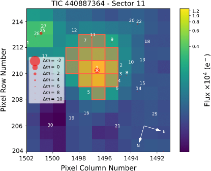
Figure 1: Target Pixel File (TPF) from TESS centered on TOI-836 from the Gaia catalog, with Gaia DR2 sources indicated by red circles with scaled magnitudes, where the numbers indicate ranked distance from the target represented by a white cross. The aperture mask is outlined in red.

For this work we use the Presearch Data Conditioning Simple Aperture Photometry (PDC-SAP) light-curve produced by the SPOC pipeline. The PDC-SAP light-curves have non-astrophysical trends removed from the raw Simple Aperture Photometry (SAP) light-curves using the PDC algorithm (Stumpe et al., 2012; Stumpe et al., 2014; Smith et al., 2012). The PDC-SAP light-curves for TOI-836 were retrieved from the Mikulski Archive for Space Telescopes (MAST) portal and used in our joint model in Section 3.

To mitigate for the effects of stellar variability on the transit lightcurves in the Sector 11 and Sector 38 TESS data, we apply a Gaussian Process (GP) model using the PyMC3 and celerite packages. We constrain this GP model for each sector using three hyperparameters as priors set up with log(s2) (a jitter term describing the excess white noise, Salvatier et al. 2016a) and log(Sw4) as normal distributions with a mean equal to the variance of the flux of each sector and a standard deviation of 0.1 for Sector 11 and 0.05 for Sector 38 (this is done to prevent overfitting of the GP); and the same is applied to log(w0). log(Sw4) and log(w0) both represent terms that describe the non-periodic variability of the light-curves (Salvatier et al., 2016a). These hyperparameter setups are identical to those described for TOI-431 in Osborn et al. (2021) and informed by the exoplanet and PyMC3 documentation. These hyperparameters are then incorporated into the SHOTerm kernel within the exoplanet framework, representing a stochastically-driven simple harmonic oscillator (Foreman-Mackey et al., 2021a). The GP model is then subtracted from the PDC-SAP flux to recover a flattened light curve from which transit models of TOI-836 b and TOI-836 c can be drawn. The effect of this can be seen in the first and second panels of Figure 3 for Sector 11 and Sector 38 of TESS respectively. We also plot the phase-folded TESS data for TOI-836 b and TOI-836 c in Figure 3 for both sectors.

For all follow-up photometry, we convert each time system to TBJD (TESS Barycentric Julian Date, BJD - 2457000) for consistency, and normalise each lightcurve by dividing by the median of the out-of-transit flux datapoints and subtracting the mean of the out-of-transit flux. The transits themselves are then modelled using a quadratic limb-darkened Keplerian orbit (with coefficients u₁ and u₂) according to Kipping (2013b), with parameters including stellar radius (R_∗) and mass (M_∗) in Solar units, planetary orbital period (P) in days, transit ephemeris (T_c) in TBJD, impact parameter (b), eccentricity (e) and argument of periastron ($\omega$) defined for each of TOI-836 b and TOI-836 c with priors informed by our spectral analysis and catalog data (see Appendices 10, 11 and 12 for details of the priors used). Transit models for each set of photometry time-series data are then created using the starry package within exoplanet, along with their corresponding planetary radii (R_p), time of the data (t) and exposure times for each instrument t_exp.

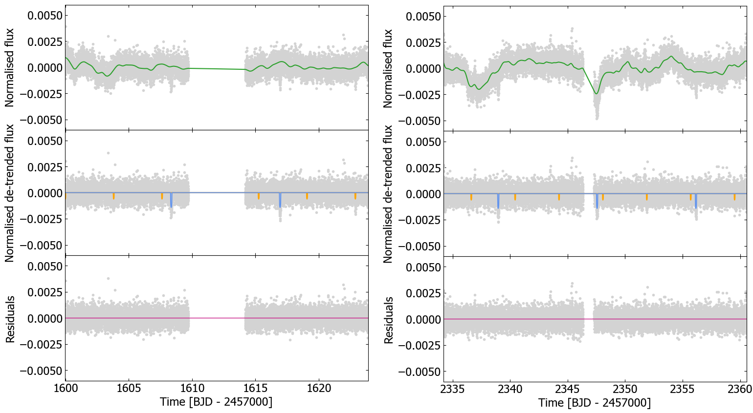
Figure 2: Top left panel: TESS PDC-SAP light curve from Sector 11 with the GP model plotted in green. Middle left panel: TESS PDC-SAP light curve data minus the GP model, with transits plotted for TOI-836 c (blue line) and TOI-836 b (orange line). Bottom left panel: Residuals between the best fit model and the TESS datapoints. Top right panel: TESS PDC-SAP light curve from Sector 38 with the GP model plotted in green. Middle right panel: TESS PDC-SAP light curve data minus the GP model, with transits plotted for TOI-836 c (blue line) and TOI-836 b (orange line). Bottom right panel: Residuals between the best fit model and the TESS datapoints.

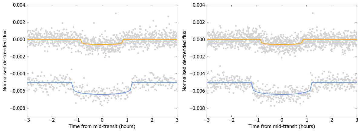
Figure 3: Left panel: TESS PDC-SAP light curve from Sector 11 minus the GP model, phase-folded to a period corresponding to that of TOI-836 b with the transit model shown in orange and phase-folded to a period corresponding to that of TOI-836 c with the transit model shown in blue. The data for TOI-836 c has been offset by -0.005 for clarity. Right panel: TESS PDC-SAP light curve from Sector 38 minus the GP model, phase folded and offset for each planet analogously to that of Sector 11.

2.2 CHEOPS photometry

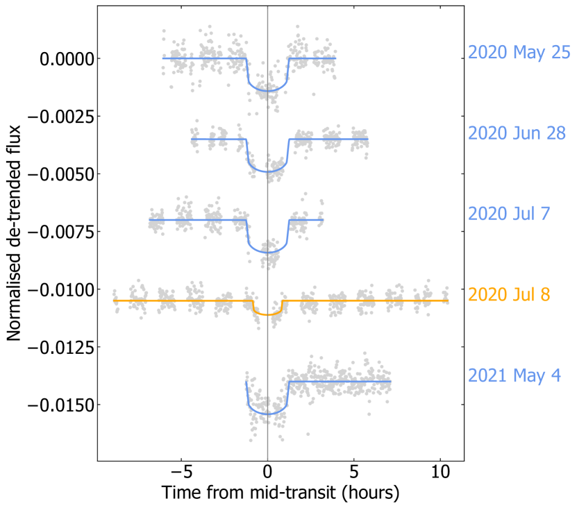
Figure 4: Light curves of TOI-836 b and TOI-836 c taken by the CHEOPS satellite as detailed in Table 2, plotted with our best fit exoplanet models for TOI-836 b in orange and TOI-836 c in blue, and offset for clarity.

The transit depths for TOI-836 b and TOI-836 c are $580$ ppm and $1140$ ppm respectively, making them challenging for photometric follow-up efforts. The CHEOPS mission is able to reach a precision of 15 ppm per 6 h for a star with V = 9 mag (Benz et al., 2021), and CHEOPS is therefore in a unique position to confirm and characterise shallow transit discoveries from TESS, as has been shown in recent publications (Bonfanti et al., 2021; Delrez et al., 2021; Leleu et al., 2021).

In order to better determine the planet radii and orbital ephemerides, and check for any TTVs, we observed TOI-836 with CHEOPS spacecraft between 2020 May 25 and 2021 May 4, as a part of the Guaranteed Time Observing programme, yielding a total of 57.81 h on target. Five observations of TOI-836 were taken by the CHEOPS satellite, resulting in the recovery of four transits of TOI-836 c, and one transit of TOI-836 b. For all visits, we use an exposure time of 60 s. See details set out in Table 2.

The CHEOPS spacecraft is in a low-Earth orbit and thus parts of the observations are unobtainable because the telescope passes through the South Atlantic Anomaly (SAA), and as the amount of stray-light entering the telescope becomes higher than the accepted threshold, our observations are interrupted by Earth occultations. These effects that occur on orbital timescales ($\sim$98.77 min) result in onboard rejections of images and manifest in a decrease in observational efficiency, corresponding to 72%, 55%, 56%, 54%, & 96% per visit, as can be seen in Figure 4.

For all visits, the data were automatically processed using the CHEOPS data reduction pipeline (DRP v13; Hoyer et al. 2020), that conducts image calibration, such as bias, gain, non-linearity, dark current, and flat fielding corrections, and performs rectifications of environmental and instrumental effects, for example cosmic-ray hits, smearing trails, and background variations. Aperture photometry is subsequently done on the corrected images using a set of standard apertures; $R$ = 22.5″ (RINF), 25.0″ (DEFAULT), and 30.0″ (RSUP), and an additional aperture that aims to optimise the radius based on contamination level and instrumental noise (ROPT). For the CHEOPS observations of TOI-836, this radius is either 29.0 or 29.5″. The DRP also computes a contamination estimate of background sources, as detailed in section 6.1 of Hoyer et al. (2020), that is subtracted from the light curves.

Due to the orbit of CHEOPS and thus the rotating field of view, CHEOPS data include short-term, non-astrophysical flux trends due to nearby contaminants, background variations, or changes in instrumental environment that vary on the timescale of the orbit of CHEOPS. Whilst previous works have used linear decorrelation with instrumental basis vectors (Bonfanti et al., 2021; Delrez et al., 2021; Leleu et al., 2021) or Gaussian process regression (Lendl et al., 2020), a recent study has shown that a novel PSF detrending method can also remove these roll angle trends (Wilson et al., 2022). In brief, this method assesses PSF shape changes over a visit by conducting a principal component analysis on the autocorrelation function of the CHEOPS subarray images, as it was found that a myriad of causes of systematic variation within CHEOPS data affects the PSF shape. A leave-one-out-cross-validation (Celisse, 2008) is used to select the most prominent components that are subsequently used to decorrelate the light curve produced by aperture photometry. We apply this method to the TOI-836 CHEOPS observations with fluxes obtained with the DEFAULT aperture. The decorrelated CHEOPS data are presented in Table 3, along with the resulting light-curves in Figure 4.

2.3 Ground-based Follow-up Photometry

Table 2: Photometric observations of TOI-836.

Instrument	Aperture	Filter	Exposure time (s)	No. of images	UT night	Planet	Epoch no.
TESS	0.105 m	TESS1	120	19527	2019 Apr 22 - 2019 May 20	TOI-836 b TOI-836 c	Epochs  1-7 Epochs  1-2
MEarth-South	0.4 m $\times$ 7	RG715	32	3054	2019 Jul 4	TOI-836 c	Epoch  8
LCOGT-SSO	1.0 m	Y	40	232	2020 Feb 29	TOI-836 c	Epoch  36
LCOGT-CTIOA	1.0 m	Y	100	138	2020 Mar 8	TOI-836 b	Epoch  83
LCOGT-SSOB	1.0 m	Y	100	109	2020 Mar 20	TOI-836 b	Epoch  86
LCOGT-SSO	1.0 m	zs	30	341	2020 Apr 12	TOI-836 c	Epoch  41
LCOGT-SSO	1.0 m	Y	100	260	2020 May 4	TOI-836 b	Epoch  98
LCOGT-SAAOC	1.0 m	zs	30	327	2020 May 16	TOI-836 c	Epoch  45
CHEOPS	0.32 m	CHEOPS2	60	398	2020 May 25	TOI-836 c	Epoch  46
CHEOPS	0.32 m	CHEOPS2	60	319	2020 Jun 28	TOI-836 c	Epoch  50
CHEOPS	0.32 m	CHEOPS2	60	318	2020 Jul 7	TOI-836 c	Epoch  51
CHEOPS	0.32 m	CHEOPS2	60	574	2020 Jul 8	TOI-836 b	Epoch  115
LCOGT-SSO	1.0 m	zs	30	345	2021 Apr 8	TOI-836 c	Epoch  83
ASTEP	0.4 m	Rc	25	370	2021 Apr 8	TOI-836 c (egress)	Epoch  83
NGTS	0.2 m $\times$ 3	NGTS3	10	5405	2021 Apr 16	TOI-836 c	Epoch  84
LCOGT-CTIO	1.0 m	zs	30	382	2021 Apr 16	TOI-836 c	Epoch  84
TESS	0.105 m	TESS1	120	19226	2021 Apr 29 - 2021 May 26	TOI-836 b TOI-836 c	Epochs  194-200   Epochs  86-88
CHEOPS	0.32 m	CHEOPS2	60	431	2021 May 4	TOI-836 c	Epoch 86
LCOGT-CTIO	1.0 m	zs	30	300	2021 Jun 24	TOI-836 c	Epoch  92

1TESS custom 600–1000 nm       2CHEOPS custom 350–1100 nm       3NGTS custom 520–890 nm

ACTIO - Cerro Tololo Inter-American Observatory     BSSO - Siding Spring Observatory     CSAAO - South Africa Astronomical Observatory

Table 3: CHEOPS photometric data for TOI-836. This table is available in its entirety online.

Time (BJD	Normalised flux	Flux uncertainty
-2457000)
1994.88704	0.99981	0.00025
1994.88773	0.99955	0.00026
1994.88843	1.00105	0.00027
1994.88912	1.00140	0.00030
1994.88982	1.00033	0.00035
1994.90649	0.99897	0.00027
1994.90718	0.99896	0.00026
1994.90788	1.00011	0.00025
1994.90857	1.00045	0.00025
…	…	…

2.3.1 MEarth-South photometry

A transit of TOI-836 c was observed using the MEarth-South telescope array (Irwin et al., 2015a) at Cerro Tololo Inter-American Observatory (CTIO), Chile on 2019 July 3-4. Seven telescopes were operated defocused to a half-flux diameter of 12 pixels (10.1 ″, given the pixel scale of 0.84 ″/pix), and an exposure time of 32 s, observing continuously starting from twilight until the target set below 2 airmasses. Observations were made using an RG715 filter. A meridian flip occurred during the transit and has been taken into account in the analysis by allowing for a separate magnitude zero-point on either side of the meridian to remove any residual flat fielding error.

Data were reduced following standard procedures for MEarth-South data (e.g. Irwin et al. 2007; Irwin et al. 2015a) with a photometric extraction aperture of radius 17 pixels (14.3 ″). To account for residual colour-dependent atmospheric extinction the transit model included linear decorrelation against airmass. The edge of the photometric aperture is slightly contaminated by fainter sources, the most significant being TIC 440887361, but we estimate that this source is approximately 10.6 TESS magnitudes fainter than the target star, so the resulting dilution of the measured transit depth should be negligible. The MEarth-South light curve is shown in Figure 5 and used in the joint modeling in Section 3.2.

2.3.2 ASTEP photometry

ASTEP (Antarctic Search for Transiting ExoPlanets) is a 40 cm Newtonian telescope designed to perform high precision photometry under the extreme conditions of the Antarctic winter (Fressin et al., 2005; Daban et al., 2010; Abe et al., 2013; Guillot et al., 2015; Mékarnia et al., 2016). It is installed at the French-Italian Concordia station at Dome C, Antarctica (75${}^{\circ}\,$06’ S, 123${}^{\circ}\,$21’ E) on a summit of the high Antarctic plateau, at an altitude of 3233 m, 1100 km inland. Dome C is an ideal location for time-series observations thanks to the 4-month continuous night during the Antarctic winter and favourable weather conditions (Crouzet et al., 2010, 2018). ASTEP is equipped with a FLI Proline KAF 16801 E $\rm 4096\times 4096$ pixel CCD camera observing in an $\rm R_{c}$ band-pass, the field of view is $1^{\circ}\times 1^{\circ}$ and the pixel size is 0.9 arcsec/pixel.

We observed TOI-836 on 2021 April 8, during 5 hours between BJD 2459313.20 and 2459313.41, and we detected the second half of the transit of TOI-836 c. We scheduled the observation using a custom scheduling tool that sends queries to the TESS Transit Finder. We set the exposure time to 25 s, the cadence was 50 s, and we collected 370 frames. The median Full Width Half Maximum (FWHM) was 4.06 ″ and the airmass varied between 1.57 and 1.94. The details of the ASTEP observations are set out in Table 2. We performed differential aperture photometry using a custom data reduction pipeline based on the pipeline described in Mékarnia et al. (2016) and adapted to TESS follow-up. We used an aperture radius of 10 pixels (9.3 ″) and 8 comparison stars. The light curve RMS is 1.43 ppt and decreases to 1.2 ppt after binning the light curve with a bin size of 3 points, for a predicted transit depth of 1.38 ppt. The transit appears clearly and is on target. The ASTEP light curve is shown in Figure 5 and used in the joint modelling in Section 3.2. The ASTEP telescope is now being upgraded with two new cameras that will observe simultaneously in two colors and will provide a much better throughput (Crouzet et al., 2020).

2.3.3 NGTS photometry

We monitored a full transit of TOI-836 c on the night of 2021 April 16 using three of the NGTS (Next Generation Transit Survey; Wheatley et al., 2018) telescopes at the ESO Paranal Observatory, Chile. The observations were performed using the NGTS multi-telescope observing method described in Bryant et al. (2020) and Smith et al. (2020). NGTS consists of an array of 0.2 m robotic telescopes, each with a wide field-of-view of 8 square degrees. A custom NGTS filter of 520–890 nm is used, and images are taken using Andor iKon-L 936 cameras, which deliver a plate-scale of $5\,\arcsec$ pix^-1. We use an exposure time of 10 s, and with readout time this translates to a cadence of approximately 13 s. The details of the NGTS observations are set out in Table 2.

The NGTS image reduction was performed using an adapted version of the standard NGTS pipeline (Wheatley et al., 2018), which has been updated to perform aperture photometry for a single star. Comparison stars which are isolated and similar to TOI-836 in brightness and CCD position were automatically identified by the pipeline using Gaia DR2 (Gaia Collaboration et al., 2018). The resultant flux from each telescope was detrended independently against airmass, and the photometry from the three telescopes is combined into a single light curve file, which is publicly available from the ExoFOP-TESS website. The NGTS light curve is shown in Figure 5 and used in the joint modeling in Section 3.2.

2.3.4 LCO photometry

We observed three full transits of TOI-836 b and six full transits of TOI-836 c from the Las Cumbres Observatory Global Telescope (LCOGT; Brown et al., 2013) 1.0 m network. The details of the LCOGT observations are set out in Table 2. We used the TESS Transit Finder, which is a customized version of the Tapir software package (Jensen, 2013), to schedule our transit observations. The telescopes are equipped with $4096\times 4096$ SINISTRO cameras having an image scale of 0.389″ per pixel, resulting in a $26\arcmin\times 26\arcmin$ field of view. The images were calibrated by the standard LCOGT BANZAI pipeline (McCully et al., 2018), and photometric data were extracted using AstroImageJ (Collins et al., 2017). The LCOGT light curves are shown in Figure 6 for TOI-836 b and TOI-836 c, and used in the joint modelling in Section 3.2.

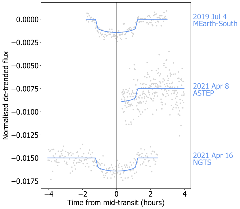
Figure 5: Lightcurves of TOI-836 c taken by the MEarth-South, NGTS and ASTEP facilities as detailed in Table 2, plotted with our best fit exoplanet models and offset for clarity.

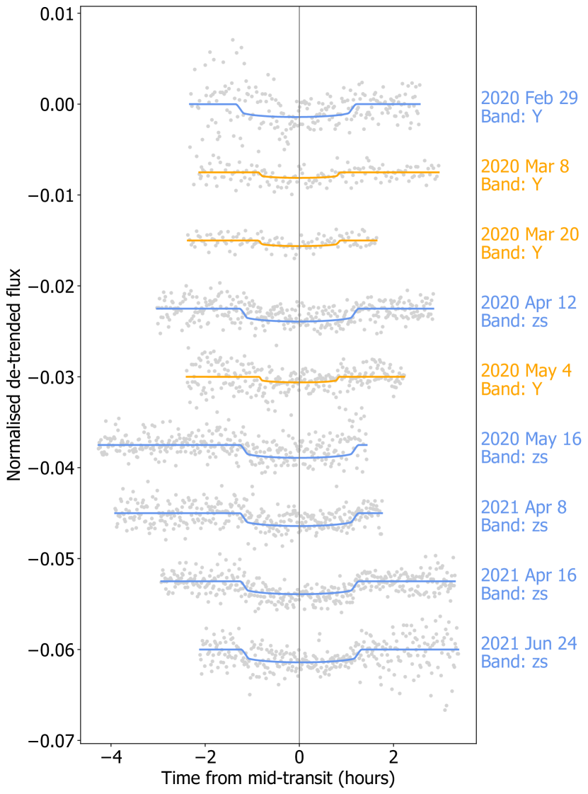
Figure 6: Light curves of TOI-836 b and TOI-836 c taken by the LCOGT network as detailed in Table 2, plotted with our best fit exoplanet models for TOI-836 b in orange and TOI-836 c in blue, and offset for clarity.

2.3.5 WASP-South photometry

The WASP-South array of 8 wide-field cameras was the Southern station of the WASP transit-search project (Pollacco et al., 2006). WASP-South observed the field of TOI-836 repeatedly over the years 2006 to 2014, observing with a broad-band filter, and accumulating a total of 93,000 photometric data points. While the precision of these observations is not sufficient to detect the transits, the long-duration monitoring is ideal for detecting photometric activity due to star spots. We thus searched the data for a rotational modulation using the methods discussed in Maxted et al. (2011). We find a persistent periodicity with a period of 22.0 $\pm$ 0.1 days, where the uncertainty estimate makes allowance for phase changes caused by changing star-spot patterns. The amplitude varies from 3 to 8 mmag and the false-alarm probability in each season’s dataset is typically $<$ 1%. In Figure 7 we show periodograms from two seasons of data, together with the resulting modulation profile from folding the data.

The 22 day period is consistent with activity seen in the TESS data, particularly in Sector 38 data (see Figure 3). We therefore adopt this as the likely spin period of the star and use it to inform our joint modelling in Section 3.2.

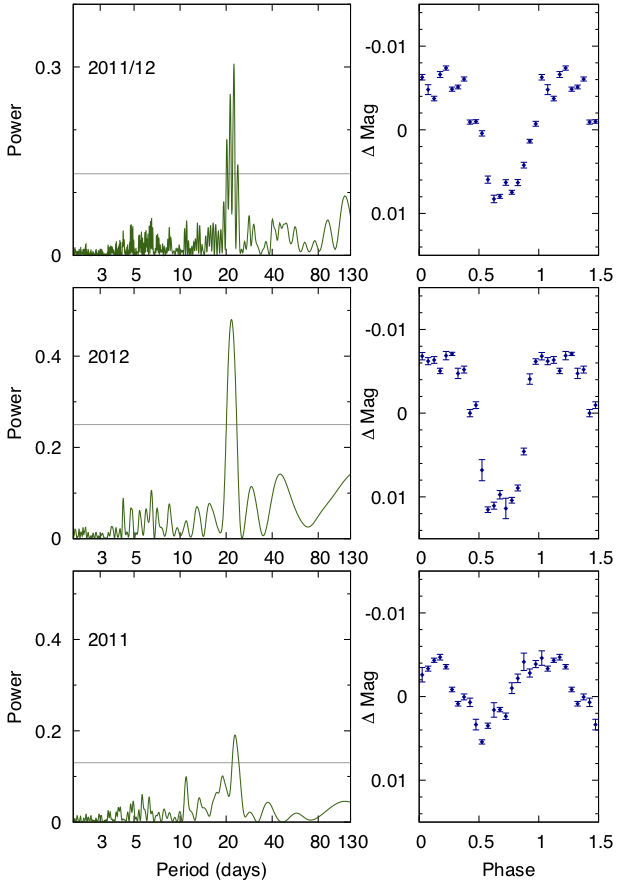
Figure 7: Left panels: Periodograms of the WASP-South lightcurves of TOI-836 from 2011 and 2012, and for 2011 & 2012 combined. The horizontal line is the estimated 1%-likelihood false-alarm level. Right panels: WASP-South photometry data, phase-folded to the best stellar rotation period estimate.

2.4 Follow-up Spectroscopy

In order to determine the stellar parameters and measure radial velocity variations, a number of spectrographs were used to observe TOI-836. Two reconnaissance spectra were taken on 2019 July 1 and 2021 May 28 with the Tillinghast Reflector Echelle Spectrograph (TRES) (Fűrész, 2008) on the 1.5 m telescope at the Fred Lawrence Whipple Observatory (FLWO). The spectra were used to derive stellar parameters using the Stellar Parameter Classification (SPC) tool (Buchhave et al., 2012, 2014). These spectra indicated that TOI-836 is a K-dwarf with a low $v\sin i_{*}$ that would be amenable to high-precision radial velocity follow-up. In this section we describe these high-precision radial velocity data, which are obtained using the HARPS and PFS spectrographs. We also obtain 11 spectra from the HIRES spectrograph (Vogt & Penrod, 1988), taken from 2009 April 6 to 2013 February 3, which we use to examine long-term radial velocity trends. The iSHELL radial velocities were taken at 2.3 microns, and as we do not implement a chromatic RV analysis as in Cale et al. (2021), we exclude them from our analysis. Additional radial velocity data from MINERVA-Australis also exist, but the lower precision of these data mean that we omit them from our analysis.

2.4.1 HARPS radial velocity observations

HARPS (High Accuracy Radial velocity Planet Searcher; Mayor et al., 2003) is an Echelle spectrograph mounted on the ESO 3.6 m telescope situated at La Silla Observatory, Chile. A total of 52 spectra of TOI-836 were obtained with HARPS as part of the NCORES program (PI D. Armstrong, 1102.C-0249). 15 of these spectra were obtained from 2020 March 16 to 2020 March 23 (7 nights), followed by a further 37 spectra from 2021 January 22 to 2021 March 2 (39 nights). These data were obtained in HARPS High-Accuracy Mode with a 1″ diameter fibre, standard resolution of R$\sim$115,000, and exposure times of approximately 1500 s. Raw data were reduced according to the standard HARPS data reduction software detailed in Lovis & Pepe (2007). The data table for these observations can be found in Table 4, which we use in our joint modelling (Section 3.2). The HARPS data are marked with an asterisk in Table 5.

Table 4: HARPS spectroscopic data for TOI-836. This table is available in its entirety online.

Time (BJD	RV	RV error	FWHM	Bisector	Contrast	S-indexMW
-2457000)	(m s-1)	(m s-1)	(m s-1)	(m s-1)
1924.744232	-26270.62	1.20	6479.82	59.29	42.086199	1.118916
1924.847515	-26272.89	1.13	6477.87	58.02	42.082108	1.088405
1925.765286	-26277.15	1.33	6483.37	54.98	42.104065	1.099795
1925.897310	-26278.60	1.42	6484.65	62.33	42.063377	1.035016
1926.748165	-26279.33	1.23	6481.65	63.03	42.111069	1.073716
1926.891093	-26276.88	1.25	6474.28	65.77	42.150971	1.039492
1927.807982	-26280.90	1.66	6472.36	61.35	42.201152	1.068344
1927.885303	-26283.22	1.24	6470.19	62.19	42.177954	1.035070
1928.764641	-26288.22	1.24	6465.28	65.38	42.164275	1.058810
1928.890901	-26289.86	1.37	6466.36	65.65	42.174431	1.042093
…	…	…	…	…	…	…

Table 5: Radial velocity follow-up details for TOI-836. Observations used in the joint model are marked with an asterisk.

Facility	Telescope aperture	No. of spectra	Resolution
HARPS *	3.6 m	52	115000
HIRES	10.0 m	11	60000
PFS *	6.5 m	30	130000
iSHELL	3.0 m	10	70000
MINERVA-Australis	0.7 m $\times$ 6	27	75000

• Sources: HARPS (Mayor et al., 2003), HIRES (Vogt & Penrod, 1988), PFS (Crane et al., 2006), iSHELL (Rayner et al., 2012), MINERVA-Australis (Wittenmyer et al., 2018; Addison et al., 2019, 2021)

2.4.2 PFS radial velocity observations

The Planet Finder Spectrograph (PFS) (Crane et al., 2006; Crane et al., 2008, 2010) is a high resolution optical Echelle spectrograph mounted on the 6.5 m Magellan II Telescope at Las Campanas Observatory, Chile. PFS is calibrated via an iodine-cell, and raw data are reduced to 1D spectra and relative radial velocities extracted using a custom pipeline based on Butler et al. (1996). The spectrograph was upgraded in 2018, and now operates with a default slit width of 0.3 ″, which delivers a resolving power of R$\sim$130,000.

TOI-836 was observed as part of the Magellan-TESS Survey (Teske et al., 2021) between 2019 July 10 to 2020 March 17. Exposure times were approximately 900-1200 s per individual observation, and usually two observations were taken per night (separated by $\sim$2 hours) and binned together. In total, 38 binned radial velocities were published in Teske et al. for TOI-836, and these are set out in table 4 of Teske et al. (2021). We use the PFS radial velocities in our joint modelling (Section 3.2). The PFS data are marked with an asterisk in Table 5.

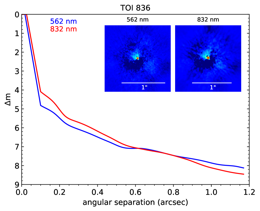
Figure 8: Reconstructed images and speckle sensitivity curves of TOI-836 taken on 2020 March 13 using Zorro on the Gemini-South 8.0 m telescope at Cerro Pachón, Chile, in each of the two bandpasses. No close companions are visible brighter than a contrast of 5 mag for separations between 0.2 and 1.2 ″. Other direct imaging data also place similar constraints on the presence of close companions.

2.4.3 HIRES radial velocity observations

HIRES (High Resolution Echelle Spectrometer; Vogt & Penrod, 1988) is an R$\sim$60,000 resolving power spectrograph mounted on the 10 m Keck Telescope at Mauna Kea Observatory, Hawaii. Like PFS, HIRES also operates with an iodine-cell wavelength calibration, and data are reduced using a custom pipeline based on Butler et al. (1996).

TOI-836 was observed as part of the Lick-Carnegie Exoplanet Survey (Butler et al., 2017) between 2009 April 6 to 2013 February 3. In total, 11 observations were made over this four year time period, with a typical exposure time of approximately 500 sec. These data are set out in table 1 of Butler et al. (2017). The observations were made prior to the discovery of the transiting planets TOI-836 b and TOI-836 c. The low cadence of these observations, coupled with the stellar activity of TOI-836, means that we decided not to use them in our GP-based joint model of Section 3.2 - however they do enable us to study any long-term radial velocity trends for the system (see Section 3.2.4).

2.5 Imaging

The large size of the TESS pixels (21$\arcsec$) necessitates a careful study of neighbouring regions in order to determine if there are stars blended in to the TESS photometric data. In such cases, planet transits can be mimicked by other stellar configurations (e.g., Lillo-Box et al. 2012; Howell et al. 2011; Lillo-Box et al. 2014; Furlan et al. 2017). Gaia shows TOI-836 to be a relatively isolated star, with no neighbours with $\Delta\,T_{mag}\,<\,6$ in the photometric aperture to within its sensitivity limits (see Figure 1). To probe regions very close to TOI-836 (< 1.5 ″), where Gaia is known to be incomplete, we use direct imaging from large ground-based telescopes.

TOI-836 was imaged by multiple telescopes and instruments in order to check for close companions. This imaging includes Gemini-Zorro and Gemini-’Alopeke (Scott et al., 2021), VLT-NaCo (Rousset et al., 2003), Keck-2-NIRC2 (Ciardi et al., 2015) and SOAR-HRCam (Ziegler et al., 2020). These imaging data are publicly available from the ExoFOP-TESS website. The conclusion from all of these imaging data is that TOI-836 has no close companions outside a separation of 0.2 ″.

As an example of this direct imaging data, Figure 8 shows the reconstructed images and speckle sensitivity curves from the observation taken using the Zorro instrument (Scott et al., 2021) on Gemini-South at Cerro Pachón Observatory, Chile. This imaging was taken on 2020 March 13 in two simultaneous passbands (562 nm and 832 nm), and like all the direct imaging, shows that TOI-836 is an isolated star to within the 5 $\sigma$ contrast limits.

3 Methods and Results

3.1 Stellar analysis

To determine the stellar parameters for TOI-836, we co-add the 52 HARPS spectra (Section 2.4.1) into a single combined spectrum with a signal-to-noise of $\sim$400 at 550 nm. We use the method described in Sousa (2014) and Santos et al. (2013) in order to derive the stellar atmospheric parameters including a trigonometric surface gravity $\log g$, effective temperature T_eff and metallicity [Fe/H]. This method measures the equivalent widths of iron lines in the combined HARPS spectrum via the ARES v2 code (Sousa et al., 2015). The abundances are then estimated using the MOOG code (Sneden, 1973) for radiative transfer, which includes a grid of model atmospheres from Kurucz (1993), and we find the best set of spectroscopic parameters by assuming equilibriums of ionization and excitation. Following the same methodology as described in Sousa et al. (2021), we use the Gaia EDR3 parallax and estimate the trigonometric surface gravity. This spectral analysis shows that TOI-836 is a K-dwarf with a $\log g$ = $4.743\pm 0.105$ dex and a T_eff = $4552\pm 154$ K. We find a metallicity of [Fe/H] = $-0.284\pm-0.067$ dex and a $v\sin i_{*}$ = $1.86\pm 0.50$ km s^-1.

To obtain the radius of TOI-836, we use a Markov-Chain Monte Carlo (MCMC) modified infrared flux method (IRFM; Blackwell & Shallis 1977; Schanche et al. 2020). This is done by building spectral energy distributions (SEDs) from atlas Catalogue stellar atmospheric models (Castelli & Kurucz, 2003) and stellar parameters derived via our spectral analysis, and calculating synthetic fluxes by integrating the SEDs over bandpasses of interest after attenuation to account for extinction. These fluxes are compared to observed broadband photometry retrieved from the most recent data releases for the following bandpasses; Gaia G, G_BP, and G_RP (Gaia Collaboration et al., 2021b), 2MASS J, H, and K (Skrutskie et al., 2006), and WISE W1 and W2 (Wright et al., 2010) to calculate the apparent bolometric flux, and hence the stellar angular diameter and effective temperature. By converting the angular diameter to the stellar radius using the offset-corrected Gaia EDR3 parallax (Lindegren et al., 2021), we obtain R_∗ = $0.666\pm 0.010$ R_⊙.

Starting from the basic input set given by (T_eff, [Fe/H], R_∗), we then derived the isochronal mass M_∗ and age $t_{*}$. To provide robust estimates, we employed two different evolutionary models, namely PARSEC v1.2S (Marigo et al., 2017) and CLES (Code Liègeois d’Évolution Stellaire, Scuflaire et al., 2008). In detail, we derived a first pair of mass and age values using the isochrone placement technique (Bonfanti et al., 2015, 2016), which we applied to pre-computed tables of PARSEC tracks and isochrones. Besides the basic input set, we further inputted the $v\sin{i_{*}}$ value to improve the convergence of the interpolating routine as detailed in Bonfanti et al. (2016). A second pair of mass and age estimates was instead retrieved through the CLES code, which generates the best stellar evolutionary track that reproduces the basic input set following the Levenberg-Marquadt minimisation scheme (Salmon et al., 2021). After carefully checking the mutual consistency of the two respective pairs of values through the $\chi^{2}$-based criterion outlined in Bonfanti et al. (2021), we finally merged the two output mass and age distributions and we obtained M_∗ = $0.678_{-0.041}^{+0.049}$ M_⊙  and $t_{*}=$$5.4^{+6.3}_{-5.0}$ Gyr. We use these values of the stellar mass and radius as priors within our exoplanet modelling (described in Section 3.2), which are then fit for in the code to produce the final values seen in Table 6.

Further to this, we derive stellar abundances using the curve-of-growth analysis method in local thermodynamic equilibrium, as employed in Adibekyan et al. (2012); Adibekyan et al. (2015). We are unable to derive reliable values for the abundances of C and O because the lines for those elements become very weak and blended with other species for cool dwarf stars, as it is in the case of TOI-836 (see eg. Delgado Mena et al. 2021). The values of [Mg/H] and [Si/H] are $-0.23\pm 0.17$ dex and $-0.29\pm 0.20$ dex respectively. These are typical values for a thin-disk star, which agrees with our calculated Galactic space velocity components and thin-disk membership probability as described in the next paragraph. There is no evidence in the stellar spectrum (such as a strong Li line) to suggest that TOI-836 is a young star. The full set of results from our spectral analysis are set out in Table 6.

Following the formulation of Johnson & Soderblom (1987), and using the values of proper motion and parallax from Gaia EDR3 (see Table 1) and a radial velocity from Gaia DR2 of $-26.603\pm 0.922$ km s^-1 (Gaia Collaboration et al., 2018), we calculate the values and uncertainties for $U$, $V$ and $W$, the heliocentric velocity components of the Galactic space velocities, in the direction of the galactic centre, rotation, and pole respectively, in Table 6. We should note that we do not subtract the Solar motion and compute the $U$, $V$ and $W$ values in the right-handed system.

We also use the approach of Reddy et al. (2006) in a Monte Carlo fashion with 100,000 samples to determine the probability that TOI-836 is in a given kinematic Galactic family, using a weighted average of the results obtained using the velocity dispersion standards of Bensby et al. (2003); Bensby et al. (2014), Reddy et al. (2006), and Chen et al. (2021). We find a Galactic thin disk membership probability for TOI-836 of 98.9%, thick disk membership probability of 1.1%, and halo membership probability of 0%. This agrees well with the Galactic eccentricity of TOI-836 of 0.08, and the high Galactic Z-component of the angular momentum of $Z$ $\approx$ 1770 kpc km s^-1. We compute these values using the galpy package after a Galactic orbit determination using the Gaia EDR3 position, proper motions, and parallax, and Gaia DR2 radial velocity integrating over 5 Gyr, as well as the typical values for [Mg/H] and [Si/H] from stellar analysis.

3.2 Exoplanet data analysis

We model the photometric and spectroscopic data presented in Section 2 using the exoplanet package (Foreman-Mackey et al., 2021a, c), which incorporates starry (Luger et al., 2019a), celerite (Foreman-Mackey et al., 2017) and PyMC3 (Salvatier et al., 2016b) within its framework. We have selected the high-quality follow-up light curves, which includes all observations from TESS and CHEOPS as our space-based photometry, one observation from NGTS, nine observations from LCOGT, one observation from ASTEP, and one observation from MEarth as our ground-based photometry sample (see Table 2). Our radial velocity modelling of short-term trends is comprised of data from HARPS and PFS.

3.2.1 Transit Timing Variations

In order to account for perceived transit timing variations (TTVs) on TOI-836 c in 2020 (year 2 of observation), we introduce an offset parameter T_c. This offset parameter is calculated by fitting each detrended, normalised dataset using the EXOFAST modelling tool (Eastman et al., 2013, 2019). The offset parameter represents the value of the central transit time found in EXOFAST, and $\delta$T_c  is the difference from the expected transit ephemeris. The corresponding $\delta$T_c  for each transit can be found in Table 7. We omit offset parameters for the transits of TOI-836 b taken by LCOGT, as these observations are not of sufficient precision to allow for suitably accurate determination of the offset parameter. We omit offset parameters for the LCOGT transit of TOI-836 c on 2020 February 29 and the ASTEP transit on 2021 April 8 for these same reasons. We also choose to omit transits of both planets in the TESS light-curves that occur very close to the start and end of sectors and close to the data download gap, as they are likely to be highly affected by systematics which may affect transit timings.

We plot the resulting offset for the central transit time T_c for each of TOI-836 b and TOI-836 c in Figure 9. We note that there appear to be no significant TTVs in the observed transits of TOI-836 b, however in TOI-836 c we detect an offset within the T_c values ranging from approximately 20 to 30 minutes. The presence of these TTVs is supported by observations from both the space-based CHEOPS satellite and multiple ground-based facilities. These TTV measurements alone are not enough to be able to put meaningful constraints on the mass of TOI-836 c, but with further TTV monitoring it may be possible.

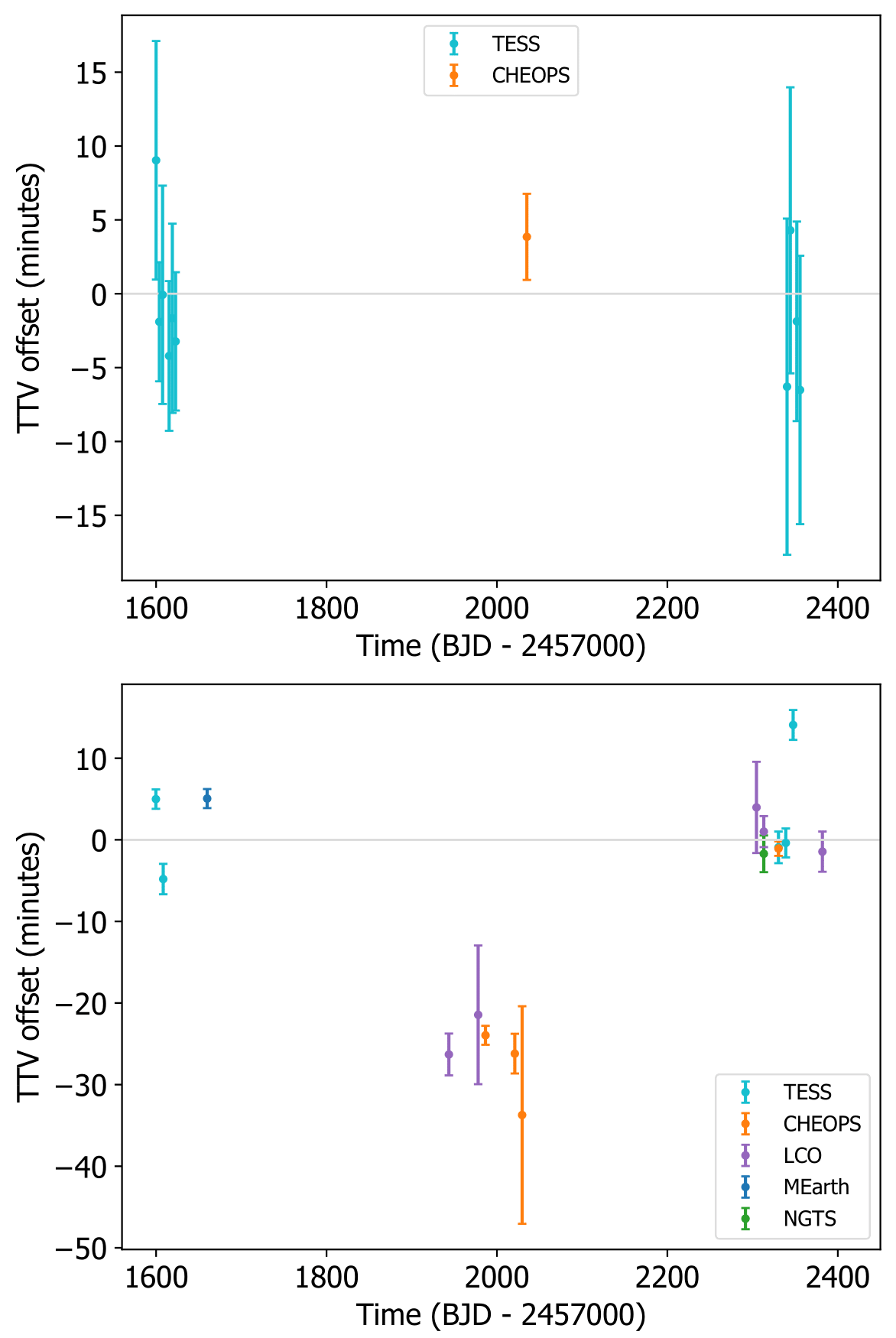
Figure 9: Top panel: Transit Timing Variations (TTVs) for each transit of TOI-836 b from the following photometry sources: TESS in turquoise and CHEOPS in yellow. Bottom panel: Transit Timing Variations (TTVs) for each transit of TOI-836 c from the following photometry sources: TESS in turquoise, CHEOPS in yellow, LCOGT in purple, MEarth-South in blue and NGTS in green.

3.2.2 Radial velocity (RV)

We model the radial velocity of TOI-836 using the HARPS and PFS data simultaneously, seen in Figure 10. We analysed these radial velocity data with various models, including linear and quadratic drift and a third planet. None of these were able to account for the large scatter in the radial velocity measurements, and therefore we find it necessary to apply a GP model for both of our chosen datasets in order to account for stellar variability. We apply a quasi-periodic kernel (commonly used in works with similar goals, such as Osborn et al. 2021), as implemented in celerite. We assign a prior probability distribution for the rotation period as a normal distribution centered around 22 days, with a standard deviation of 0.1 days, based on the results from the WASP-South periodogram. In completion, our kernel is a combination of two available kernels in the PyMC3 package (Salvatier et al., 2016b) - the Periodic and ExpQuad kernels are multiplied to create the final quasi-periodic kernel. As part of this analysis, we define a set of GP hyperparameters which are fit concurrently for both sets of radial velocity data: $\eta$ representing the GP amplitude, the stellar rotation period P, the smoothing parameter l_P and the timescale of active region evolution l_E. This has been shown to successfully model stellar activity in eg. Grunblatt et al. (2015), Santerne et al. (2018) and Osborn et al. (2021).

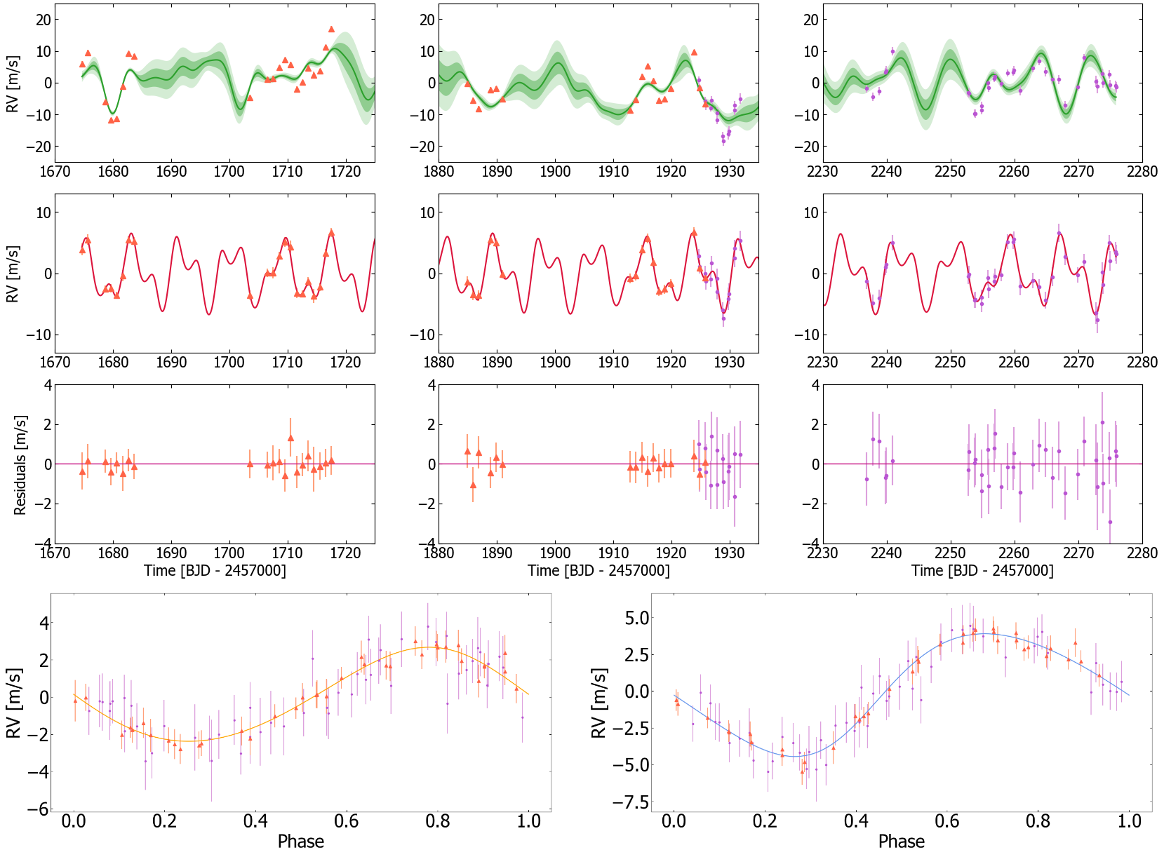
Figure 10: Top panels: HARPS (purple circles) and PFS (orange triangles) RV data with formal uncertainties with the GP model plotted as a solid green line, with 1 and 2 standard deviations in lighter shades. Second panels: Combined RV models of the two planets, with the GP subtracted, with HARPS and PFS RV datapoints. Third panels: Residuals for HARPS and PFS datapoints relative to a baseline RV of 0 m s^-1. Fourth panels (left): HARPS (purple circles) and PFS (orange triangles) RV data, phase-folded to a period corresponding to that of TOI-836 b with the RV model shown in orange. Fourth panels (right): HARPS and PFS data, phase-folded to a period corresponding to that of TOI-836 c with the RV model shown in blue.

When modelling the HARPS and PFS data, we utilise exoplanet to find values for the radial velocity semi-amplitude K with priors from 0 to 10  m s^-1. We also fit for values for the offsets as a normal distribution centered around the mean of the radial velocity of each dataset. We also fit for jitter terms centered around the minimum radial velocity error multiplied by 2, which represent other variability not accounted for in the HARPS and PFS formal uncertainties, and the application of the GP model to the data.

Modelled planetary reflex motions are subtracted from the radial velocities at each timestamp before being passed to the GP kernel, and we use the same time system for both the HARPS and PFS data sets (BJD - 2457000). The prior distributions for each of the parameters used in the code can be found in Appendices 10, 11 and 12 for the host star TOI-836, and the planets TOI-836 b and TOI-836 c respectively.

3.2.3 Joint fitting

To bring the two observational methods together, we utilise the exoplanet package to fit for our initial values from the maximum log probability, which are then passed into the PyMC3 sampler as a starting point in a No U-Turn Sampler (NUTS) variant of the Hamilton Monte Carlo (HMC) algorithm (Hoffman & Gelman, 2011). We set our run to have a burn-in of 4000 samples, 4000 steps and 10 chains, giving our modelling significant opportunity to explore the parameter spaces.

As a result of our joint fitting of transit and radial velocity data, we find that TOI-836 b is a super-Earth planet with a radius of $1.70\pm 0.07$ R_⊕ and mass of $4.5\pm 0.9$ M_⊕, on a period of $3.82$ days, and TOI-836 c is a sub-Neptune planet with a radius of $2.59\pm 0.09$ R_⊕ and mass of $9.6\pm{2.6}$ M_⊕  on a period of $8.60$ days. From this we can infer a bulk density of $5.02^{+0.36}_{-0.44}$ g cm^-3 for TOI-836 b, and $3.06^{+0.47}_{-0.54}$ g cm^-3 for TOI-836 c. A full set of parameters for TOI-836 can be found in Table 6, and parameters for each planet can be found in Table 8.

Table 6: Stellar parameters of TOI-836.

Property (unit)	Value	Source
Mass (M⊙)	$0.678_{-0.041}^{+0.049}$	exoplanet
Radius (R⊙)	$0.665\pm 0.010$	exoplanet
Density (g cm-3)	$3.294^{+0.079}_{-0.092}$	exoplanet
Prot (days)	$21.987\pm 0.097$	exoplanet
LD coefficient u1	$0.039\pm 0.235$	exoplanet
LD coefficient u2	$0.023\pm 0.335$	exoplanet
$\log g$	$4.743\pm 0.105$	ARES + MOOG + Gaia
Teff (K)	$4552\pm 154$	ARES + MOOG
$v\sin i_{*}$ (km s-1)	$1.86\pm 0.50$	ARES + MOOG
Age (Gyr)	$5.4^{+6.3}_{-5.0}$	Isochrones
Stellar abundances
[Fe/H] (dex)	$-0.284\pm-0.067$	ARES + MOOG
[Mg/H] (dex)	$-0.23\pm 0.17$	ARES + MOOG
[Si/H] (dex)	$-0.29\pm 0.20$	ARES + MOOG
Galactic space velocity components
$U$ (km s-1)	-35.6 $\pm$ 0.7	Gaia EDR3
$V$ (km s-1)	-10.7 $\pm$ 0.3	Gaia EDR3
$W$ (km s-1)	-3.50 $\pm$ 0.5	Gaia EDR3

• Sources: exoplanet (Foreman-Mackey et al., 2021a, c), ARES (Sousa et al., 2015), MOOG (Sneden, 1973; Kurucz, 1993), Gaia (Gaia Collaboration et al., 2021a)

Table 7: Timing offsets for observations of TOI-836 b and TOI-836 c.

Facility	UT night	$\delta$Tc (days)	$\delta$Tc error (days)
TOI-836 b
TESS S11	—	0.009757	0.005609
TESS S11	—	0.002165	0.002800
TESS S11	—	0.003431	0.005132
TESS S11	—	0.000558	0.003520
TESS S11	—	0.002330	0.004450
TESS S11	—	0.001242	0.003252
LCOGT-CTIO	2020 Mar 8	—	—
LCOGT-SSO	2020 Mar 20	—	—
LCOGT-SSO	2020 May 4	—	—
CHEOPS	2020 Jul 8	0.0061575	0.002024
TESS S38	—	—	—
TESS S38	—	-0.000887	0.007903
TESS S38	—	0.006464	0.006724
TESS S38	—	—	—
TESS S38	—	0.0021850	0.004691
TESS S38	—	-0.001041	0.006310
TESS S38	—	—	—
TOI-836 c
TESS S11	—	0.0034651	0.000826
TESS S11	—	0.0033399	0.001295
MEarth-South	2019 Jul 4	0.0035104	0.000811
LCOGT-SSO	2020 Feb 29	—	—
LCOGT-SSO	2020 Apr 12	0.0182677	0.001780
LCOGT-SAAO	2020 May 16	-0.0148950	0.005903
CHEOPS	2020 May 25	-0.0166364	0.000806
CHEOPS	2020 Jun 28	-0.0181972	0.001690
CHEOPS	2020 Jul 7	-0.0234211	0.000923
LCOGT-SSO	2021 Apr 8	0.0027583	0.003884
ASTEP	2021 Apr 8	—	—
NGTS	2021 Apr 16	-0.0011893	0.001562
LCOGT-CTIO	2021 Apr 16	0.0007001	0.001320
LCOGT-CTIO	2021 Jun 24	-0.0010068	0.001712
CHEOPS	2021 May 4	0.0007432	0.000622
TESS S38	—	-0.0006412	0.001347
TESS S38	—	-0.0002651	0.001231
TESS S38	—	0.0097779	0.001272

• Sources: LCOGT (Brown et al., 2013), CHEOPS (Benz et al., 2021), ASTEP (Daban et al., 2010), NGTS (Wheatley et al., 2018), MEarth-South (Irwin et al., 2015b), TESS (Ricker et al., 2015)

Table 8: Parameters of TOI-836 b  and TOI-836 c.

Property	Value
	TOI-836 b	TOI-836 c
Identifier	TOI-836.02	TOI-836.01
Period (days)	$3.81673\pm 0.00001$	$8.59545\pm 0.00001$
Mass (M⊕)	$4.53^{+0.92}_{-0.86}$	$9.6^{+2.7}_{-2.5}$
Radius (R⊕)	$1.704\pm 0.067$	$2.587\pm 0.088$
Density (gccc)	$5.02^{+0.36}_{-0.44}$	$3.06^{+0.48}_{-0.54}$
Rp/R*	$0.0235\pm 0.0013$	$0.0357\pm 0.0018$
Tc (TBJD)	$1599.9953\pm 0.0019$	$1599.7623\pm 0.0008$
T1-T4 duration (hours)	$1.805^{+0.222}_{-0.007}$	$2.486^{+0.161}_{-0.192}$
T2-T3 duration (hours)	$1.6823^{+0.0012}_{-0.3292}$	$2.256^{+0.144}_{-0.432}$
Impact parameter	$0.58\pm 0.11$	$0.53\pm 0.13$
K (m s-1)	$2.38\pm 0.35$	$3.86\pm 0.85$
Inclination (∘)	$87.57\pm{0.44}$	$88.7\pm{1.5}$
Semi-major axis (AU)	$0.04220\pm 0.00093$	$0.0750\pm 0.0016$
Temperature Teq (K) *	$871\pm 36$	$665\pm 27$
Insolation flux (S⊙)	$78.838\pm 0.015$	$26.707\pm 0.003$
Eccentricity	$0.053\pm 0.042$	$0.078\pm 0.056$
Argument of periastron (∘)	$9\pm 92$	$-28\pm 113$
TSM	$65.7\pm 5.8$	$82.4\pm 5.8$

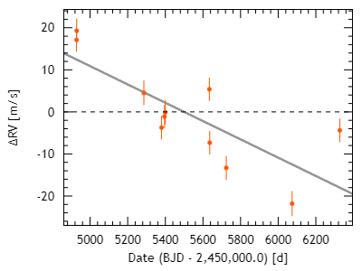
Figure 11: Radial velocity data of TOI-836 from the HIRES instrument on the Keck telescope from 2009 April 6 to 2013 February 3, and fit with a linear trend represented by the solid grey line.

3.2.4 Long-term trends

In addition to our short-term radial velocity analysis with data from HARPS and PFS, we also make use of HIRES data to constrain longer-term trends. We fit the data for a linear drift, and find a drift value of $-7.95\pm 2.14$ m s^-1 yr^-1. The fit is shown in Figure 11. The HIRES data is sparsely sampled over a duration of approximately four years. Therefore it is not possible to remove the stellar activity signal in the manner we did for the HARPS and PFS data, and so the marginally detected linear trend may not be real, and we do not use this trend when fitting the radial velocities in Section 3.2.2. However the HIRES data is able to rule out any radial velocity drift above the level of the stellar activity signal ($\sim$ 10 m s^-1) over a four year time period.

4 Discussion

In addition to the results from our joint modelling, we find that TOI-836 has a relatively low metallicity of [Fe/H] = $-0.284\pm-0.067$ dex. As was found in Adibekyan et al. (2021), there is a strong trend between host stellar metallicity and the iron component for low-mass exoplanets. This can be interpreted as systems that formed from metal-rich proto-stellar/planetary disks have stars with metal-rich photospheres and planets with large metallic cores. This is supported by the recent study of Wilson et al. (2022) that found a correlation between sub-Neptune planet densities and stellar metallicities across all stellar types that implies that sub-Neptunes around metal-rich stars have larger metallic cores that can retain a larger atmosphere and hence appear less dense. This effect has also been observed in radius valley trends with metallicity (Chen et al., 2022). As TOI-836 has a low-metallicity we reproduce Fig. 15 of Wilson et al. (2022) and plot the bulk densities of the two planets against the stellar metallicity in Figure 12, alongside a sample of planets orbiting K-dwarfs with a radius of $<$4 R_⊕ and a density of $<$15 g cm^-3 from the NASA Exoplanet Archive. This sample of all well-characterised super-Earths and sub-Neptunes around K-dwarfs supports previous findings and strengthens the evidence that stellar composition affects planetary internal structure.

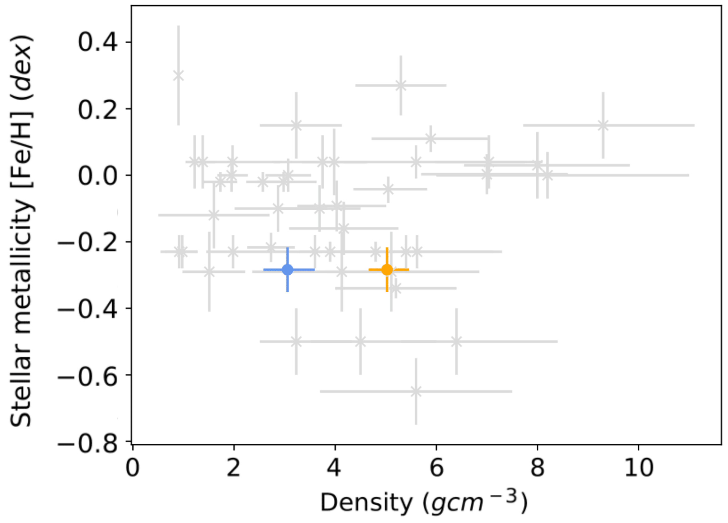
Figure 12: Bulk densities of TOI-836 b (orange) and TOI-836 c (blue) plotted against the stellar metallicity of TOI-836, along with a sample of planets orbiting K-dwarfs with R$<$4 R_⊕ and $\rho$ $<$15 g cm^-3.

4.1 Positions of the planets on the mass-radius (M-R) diagram

We plot TOI-836 b and TOI-836 c on the mass-radius (M-R) diagram in Figure 13, using fancy-massradius-plot, alongside a sample of exoplanets from the TEPCAT catalog (Southworth, 2011). It can be seen that TOI-836 b sits directly between the MgSiO₃ and 50% Fe–50% MgSiO₃ planetary composition models from Zeng et al. (2016), and TOI-836 c sits on the H₂O track. The masses and radii of TOI-836 b and TOI-836 c, along with their bulk densities, are consistent with the previously-determined populations of super-Earths and mini-Neptunes.

Figure 13: Mass-radius diagram plotted for TOI-836 b in orange and TOI-836 c  with exoplanets from the TEPCAT catalog (Southworth, 2011) in grey and composition models from Zeng et al. (2016).

4.2 Internal structure modelling

Using the planetary and stellar parameters derived above, we used a Bayesian analysis to infer the internal structure of both planets. The method we use is presented in detail in Leleu et al. (2021); we just recall here the main elements. The Bayesian analysis relies on two parts. The first one is the forward models which allows computing the planetary radius as a function of internal structure parameters, here the mass of the solid Fe/Si core, the fraction of Fe in the core, the mass of the silicate mantle and its composition (Si, Mg and Fe molar ratios), the mass of the water layer, the mass of the gas envelope (composed in this model of pure H/He), the equilibrium temperature of the planet, and its age. The second part is the Bayesian inference itself.

The details of the forward model are given in Leleu et al. (2021), we just emphasize the fact that the gaseous (H/He) part of the planet does not influence, in our model, the ‘non-gas’ part of the planet (core, mantle and water layer). The radius of the non-gas part is not influenced by the potential compression and thermal isolation effect from the gas envelope. The molar ratio of Fe, Si and Mg in the refractory parts of the two planets (core and mantle) are assumed to be identical and similar to the one of the star. Note, however, that Adibekyan et al. (2021) recently showed that the stellar and planetary abundances may not be always correlated in a one-to-one relation. The water and gas mass ratio, on the other hand, are not required to be similar between the two planets. In terms of priors, we assume that the core, mantle and water mass fraction (relative to the non-gas part) are uniform (subject to the constraint that they add up to one), whereas the mass fraction of the H/He layer is assumed to be uniform in log. We point out the fact that considering, instead, a uniform prior for the H/He gas layer would translate to more gas-rich planets, and consequently less water-rich planets.

The resulting internal structure of both planets presented are summarized in Table 9. TOI-836 b  is likely to contain a very small fraction of gas, and could have a non-negligible mass of water (although the solution with no water is also compatible with the data). TOI-836 c, on the other hand, has a much smaller density and is likely to contain more gas and/or water. We finally recall that the derived internal structure results from a Bayesian analysis, and that the distributions are of statistical nature and depend somewhat on the assumed priors.

The structure of TOI-836 b is somewhat analogous to that of TOI-1235 b (Cloutier et al., 2020), despite the difference in the host star’s spectral type, and the rocky composition of the planet may support a thermally-driven or core-powered mass loss scenario rather than a gas-poor formation scenario. TOI-836 c on the other hand is a little more ambiguous, but given its insolation flux of $26.707\pm 0.003$ S_⊙ and radius of $2.59\pm 0.09$ R_⊕, we expect a non-negligible fraction of its mass to be in gaseous form.

These two planets may also support the concept of intra-system uniformity reported by Millholland et al. (2017) and Millholland & Winn (2021), as the two planets lie close together within the mass-radius space than if two planets were to be drawn at random from the entire distribution of exoplanets according to their radii.

Table 9: Interior structure properties of TOI-836 b and TOI-836 c.

Property (unit)	Values
	TOI-836 b	TOI-836 c
Mcore/Mtotal	$0.12^{+0.16}_{-0.11}$	$0.10^{+0.15}_{-0.09}$
Mwater/Mtotal	$0.18^{+0.25}_{-0.16}$	$0.33^{+0.15}_{-0.28}$
log(Mgas)	$-8.33^{+3.95}_{-3.30}$	$-1.99^{+0.93}_{-6.77}$
Fecore	$0.90^{+0.09}_{-0.08}$	$0.90^{+0.09}_{-0.08}$
Simantle	$0.41^{+0.08}_{-0.07}$	$0.41^{+0.08}_{-0.07}$
Mgmantle	$0.45^{+0.15}_{-0.17}$	$0.44^{+0.15}_{-0.17}$

4.3 Positions of the planets compared to the radius valley

The radius valley is a bimodal distribution of planetary radii that separates super-Earths and sub-Neptunes either side of R_p $\approx$ 2 R_⊕ (Van Eylen et al., 2018; Fulton et al., 2017), from $\approx$ 1.3 R_⊕ and $\approx$ 2.6 R_⊕, respectively. The radius valley is important to examine on the basis of its implications for the formation and evolution of terrestrial planets (Giacalone et al., 2022). Some commonalities can be found within the population of super-Earths on the left side of the valley, consisting of atmosphere-stripped rocky cores, and the population of mini-Neptunes on the right hand side, consisting of rocky cores that have retained their atmospheres (Van Eylen et al., 2021). Many possibilities for the origin of the radius valley have been speculated, including the theory that terrestrial planets lose their atmospheres through photoevaporation (Owen & Wu, 2013; Jin & Mordasini, 2017; Van Eylen et al., 2021), mass loss due to core temperatures (Ginzburg et al., 2016), and the impacts of planetesimals (Schlichting et al., 2015).

In Figure 14 we plot a histogram of planets with orbital periods less than 100 days based on data from Fulton & Petigura (2018), along with the positions of TOI-836 b and TOI-836 c using the modelled values from exoplanet in Table 8. We also plot a diagram of planetary radius against the insolation fluxes in Figure 15, alongside a sample of the exoplanet population and the position of the radius valley as estimated by Martinez et al. (2019). TOI-836 b can be seen to sit directly within this valley, and TOI-836 c can be seen close to the peak on the higher radius side of the valley. TOI-836 b is set at a particularly interesting location, and there may be scope for further investigation of the extent and composition of its atmosphere, especially as the host star is suspected to not be young in age (see Section 3.1).

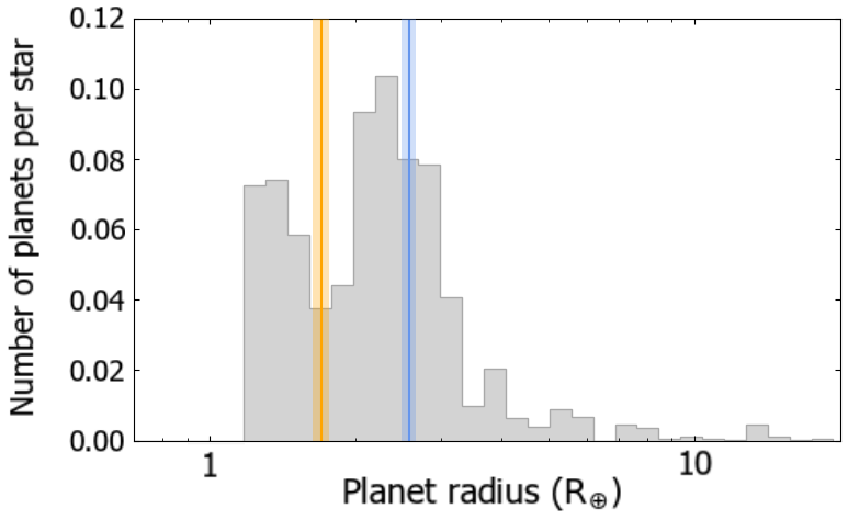
Figure 14: Histogram of confirmed planets with periods less than 100 days, using data from Fulton & Petigura (2018) represented in grey, overplotted with the radii of TOI-836 b in orange and TOI-836 c in blue, including 1$\sigma$ standard deviations according to Table 8.

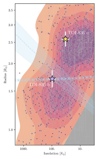
Figure 15: TOI-836 b and TOI-836 c (filled stars) as a function of planetary radius and insolation, compared with the population of exoplanets. Colours represent a kernel density estimation (KDE) applied to small (R_p $<$ 4 R_⊕), transiting planets retrieved from the NASA Exoplanet Archive (Akeson et al., 2013b). The dashed line (and associated 1-$\sigma$ error band) shows the estimate for the position of the evaporation valley from Martinez et al. (2019), while the dotted line shows a boundary due to gas-depleted formation derived from cool stars in Kepler and K2, converted to insolation using stellar parameters for TOI-836 (Cloutier & Menou, 2020).

In order to evaluate TOI-836 as a potential target for transmission spectroscopy follow-up in the era of JWST (James Webb Space Telescope; Gardner et al., 2006), we calculate a Transmission Spectroscopy Metric (TSM) for each of the planets based upon equation 1 in Kempton et al. (2018). This value is an estimate of the observed SNR of each planet as would be achieved by the NIRSPEC instrument on JWST. We find a TSM for TOI-836 b of $65.7$, and a TSM for TOI-836 c of $82.4$ (see Table 8). We also note that the system has been allocated time on JWST as can be seen in Batalha et al. (2021), with the intention of further examining the atmospheric characteristics of TOI-836 b and TOI-836 c through molecular abundances. The precise masses provided in this paper will greatly help in the characterisation of the atmospheres of these planets.

5 Conclusion

In this paper, we have presented the TOI-836 system and the discovery of its two planets, TOI-836 b and TOI-836 c. We base our discovery upon data from two sectors of TESS data (11 and 38 from year 1 and year 3 respectively) at 2-minute cadence, and a further five space-based observations ranging from 2020 to 2021 from CHEOPS, which are complemented by ground-based photometry from the NGTS, MEarth, LCOGT and ASTEP facilities, with supporting evidence for a stellar rotation period of $21.99\pm 0.097$ days supported by data from WASP-South. We model this photometry data jointly with radial velocity data from HARPS and PFS using the exoplanet package to constrain short-term trends, and HIRES data for long-term trends. We are also able to rule out the presence of blended stellar companions that may affect our photometry from an examination of the imaging from Gemini-Zorro. The planets orbit a K-type dwarf star with a mass of $0.68\pm 0.05$ M_⊙ and a radius of $0.67\pm 0.01$ R_⊙.

TOI-836 b is a super-Earth planet with a mass of $4.5\pm 0.9$ M_⊕ and a radius of $1.70\pm 0.07$ R_⊕, on an orbit of $3.82$ days. Our internal structure modelling indicates that this planet possesses a relatively small fraction of its mass in the form of gas.

TOI-836 c is a sub-Neptune with a mass of $9.6\pm{2.6}$ M_⊕and a radius of $2.59\pm 0.09$ R_⊕, on an orbit of $8.60$ days. Our structure modelling indicates that it contains a higher proportion of gas and/or water than TOI-836 b. We also find significant Transit Timing Variations within our observations of this planet, which may indicate the presence of a third non-transiting planet in the system - however we find no transits of a third planet within our current set of photometry data, or any indication of an additional periodic signal in our current radial velocity data.

TOI-836 b appears in the centre of the radius valley, and TOI-836 c appears to sit close to the peak on the right hand side of the valley, which is an area of interest in terms of the formation and structure of terrestrial planets and the dynamics of atmospheric loss and retention. The planets also contribute to the TESS Level 1 Mission requirement, and are particularly amenable to follow-up observations in the era of JWST.

Data Availability

The TESS data is accessible via the MAST (Mikulski Archive for Space Telescopes) portal at https://mast.stsci.edu/portal/Mashup/Clients/Mast/Portal.html. Photometry and imaging data from NGTS, MEarth, LCOGT, ASTEP and Gemini are accessible via the ExoFOP-TESS archive at https://exofop.ipac.caltech.edu/tess/target.php?id=440887364. The exoplanet modelling code and associated python scripts for parameter analysis and plotting are available upon reasonable request to the author. The posterior plots are available online as supplementary material to this publication.

Appendix A Priors

Table 10: Global fit parameter prior function type and prior limits for TOI-836.

Parameter	Prior	Value
Baseline flux	$\mathcal{N}$(0, 1)
M∗ (M⊙)	$\mathcal{N}$(0.678, 0.049, 0.65)	Table 6
R∗ (R⊙)	$\mathcal{N}$(0.666, 0.010, 0.56)	Table 6
Period (days)	$\mathcal{N}$(22, 0.1)	Table 6
LD coefficient u1	Kipping (2013b)	Table 6
LD coefficient u2	Kipping (2013b)	Table 6
TESS GP
Sector 11
Mean	$\mathcal{N}$(0, 1)	0.00006 $\pm$ 0.00021
log(s2)	$\mathcal{N}$(-14.704∗, 0.1)	-14.98064 $\pm$ 0.01205
log(w0)	$\mathcal{N}$(0, 0.1)	0.10400 $\pm$ 0.09697
log(Sw4)	$\mathcal{N}$(-14.704∗, 0.1)	-14.12245 $\pm$ 0.09004
Sector 38
Mean	$\mathcal{N}$(0, 1)	0.00008 $\pm$ 0.00031
log(s2)	$\mathcal{N}$(-13.903∗, 0.1)	-14.86420 $\pm$ 0.01063
log(w0)	$\mathcal{N}$(0, 0.05)	0.00736 $\pm$ 0.04815
log(Sw4)	$\mathcal{N}$(-13.903∗, 0.1)	-13.47408 $\pm$ 0.04995
RV GP
Amplitude	$\mathcal{C}$(5)	7.13782 $\pm$ 1.05463
lE	$\mathcal{T}$(22, 20, 20)	31.59616 $\pm$ 5.63098
lP	$\mathcal{T}$(0.1, 10, 0, 1)	0.21018 $\pm$ 0.02573
HARPS offset	$\mathcal{N}$(-26274.131†,10)	-26144.6 $\pm$ 2622.4
log(Jitter)HARPS	$\mathcal{N}$(0.247‡,5)	-3.01818 $\pm$ 3.12178
PFS offset	$\mathcal{N}$(0.403†,10)	-0.75678 $\pm$ 1.72435
log(Jitter)PFS	$\mathcal{N}$(-1.270‡,5)	-1.51981 $\pm$ 3.07024

• Prior distributions:

• (lower limit x, upper limit y) for uniform distribution $\mathcal{U}$(x,y)

• (mean $\mu$, standard deviation $\sigma$, test value $\alpha$) for normal distribution $\mathcal{N}$($\mu$,$\sigma$,$\alpha$)

• (mean $\mu$, standard deviation $\sigma$, lower limit x, upper limit y) for truncated normal distribution $\mathcal{T}$($\mu$,$\sigma$,x,y)

• (scale parameter $\beta$) for half-Cauchy distribution $\mathcal{C}$($\beta$)

• Prior values:

• ^∗ Equivalent to the log of the variance of the TESS flux from the corresponding sector

• ^† Equivalent to the mean of the radial velocity from the corresponding spectrographs

• ^‡ Equivalent to 2 times the log of the minimum radial velocity error from the corresponding spectrographs

Table 11: Global fit parameter prior function type and prior limits for TOI-836 b.

Parameter	Prior
TOI-836 b
Period (days)	$\mathcal{U}$(3.7, 3.9)
Transit ephemeris (TBJD)	$\mathcal{U}$(2458599.98, 2458600.03)
KRV (m s-1)	$\mathcal{U}$(0, 10)
log(Rp)	$\mathcal{N}$(-4.062§, 1)
b	$\mathcal{U}$(0, 1)
e	Kipping (2013a), $\mathcal{B}$(e, 0.867, 3.03)
$\omega$ (rad)	$\mathcal{U}$($-\pi,\pi$)

• Numbers in brackets represent:

• (lower limit x, upper limit y) for uniform distribution $\mathcal{U}$(x,y)

• (mean $\mu$, standard deviation $\sigma$, test value $\alpha$) for normal distribution $\mathcal{N}$($\mu$,$\sigma$,$\alpha$)

• Distributions for eccentricity e are built into the exoplanet package and based on Kipping (2013a) which includes the Beta distribution $\mathcal{B}$(e,a,b) (exponential e, shape parameter a, shape parameter b)

• § Equivalent to 0.5$\times$log($\delta$)+log(R_∗), $\delta$ represents transit depth (based on ExoFOP catalog values)

Table 12: Global fit parameter prior function type and prior limits for TOI-836 c.

Parameter	Prior
TOI-836 c
Period (days)	$\mathcal{U}$(8.5, 8.7)
Transit ephemeris (TBJD)	$\mathcal{U}$(2458599.74, 2458599.79)
KRV (m s-1)	$\mathcal{U}$(0, 10)
log(Rp)	$\mathcal{N}$(-3.701§, 1)
b	$\mathcal{U}$(0, 1)
e	Kipping (2013a), $\mathcal{B}$(e, 0.867, 3.03)
$\omega$ (rad)	$\mathcal{U}$($-\pi,\pi$)

• Numbers in brackets represent:

• (lower limit x, upper limit y) for uniform distribution $\mathcal{U}$(x,y)

• (mean $\mu$, standard deviation $\sigma$, test value $\alpha$) for normal distribution $\mathcal{N}$($\mu$,$\sigma$,$\alpha$)

• Distributions for eccentricity e are built into the exoplanet package and based on Kipping (2013a) which includes the Beta distribution $\mathcal{B}$(e,a,b) (exponential e, shape parameter a, shape parameter b)

• § Equivalent to 0.5$\times$log($\delta$)+log(R_∗), $\delta$ represents transit depth (based on ExoFOP catalog values)

Appendix B Author affiliations

¹ Department of Physics, University of Warwick, Gibbet Hill Road, Coventry CV4 7AL, UK
² Centre for Exoplanets and Habitability, University of Warwick, Gibbet Hill Road, Coventry CV4 7AL, UK
³ Centre for Exoplanet Science, SUPA School of Physics and Astronomy, University of St Andrews, North Haugh, St Andrews KY16 9SS, UK
⁴ Space Research Institute, Austrian Academy of Sciences, Schmiedlstrasse 6, A-8042 Graz, Austria
⁵ Instituto de Astrofísica e Ciências do Espaço, Universidade do Porto, CAUP, Rua das Estrelas, 4150-762 Porto, Portugal
⁶ Departamento de Física e Astronomia, Faculdade de Ciências, Universidade do Porto, Rua do Campo Alegre, 4169-007 Porto, Portugal
⁷ Physikalisches Institut, University of Bern, Gesellsschaftstrasse 6, 3012 Bern, Switzerland
⁸ Center for Astrophysics | Harvard & Smithsonian, 60 Garden St., Cambridge, MA 02138, USA
⁹ Université Côte d’Azur, Observatoire de la Côte d’Azur, CNRS, Laboratoire Lagrange, CS 34229, F-06304 Nice Cedex 4, France
¹⁰ School of Physics and Astronomy, University of Leicester, Leicester LE1 7RH, UK
¹¹ University of Southern Queensland, Centre for Astrophysics, USQ Toowoomba, West Street, QLD 4350 Australia
¹² Instituto de Astrofisica de Canarias, 38200 La Laguna, Tenerife, Spain
¹³ Departamento de Astrofisica, Universidad de La Laguna, 38206 La Laguna, Tenerife, Spain
¹⁴ Departamento de Astronomia, Universidad de Chile, Casilla 36-D, Santiago, Chile
¹⁵ Institut de Ciencies de l’Espai (ICE, CSIC), Campus UAB, Can Magrans s/n, 08193 Bellaterra, Spain
¹⁶ Institut d’Estudis Espacials de Catalunya (IEEC), 08034 Barcelona, Spain
¹⁷ Admatis, 5. Kandó Kálmán Street, 3534 Miskolc, Hungary
¹⁸ NASA Goddard Space Flight Center, 8800 Greenbelt Road, Greenbelt, MD 20771, USA
¹⁹ University of Maryland, Baltimore County, 1000 Hilltop Circle, Baltimore, MD 21250, USA
²⁰ Depto. de Astrofísica, Centro de Astrobiología (CSIC-INTA), ESAC campus, 28692 Villanueva de la Cañada (Madrid), Spain
²¹ Center for Space and Habitability, Gesellsschaftstrasse 6, 3012 Bern, Switzerland
²² Université Grenoble Alpes, CNRS, IPAG, 38000 Grenoble, France
²³ Observatoire de Genève, Université de Genève, Chemin de Pegasi, 51, 1290 Versoix, Switzerland
²⁴ Department of Astronomy, Stockholm University, AlbaNova University Center, 10691 Stockholm, Sweden
²⁵ Programma Nazionale di Ricerche in Antartide (PNRA), Concordia station, Antarctica
²⁶ Institute of Planetary Research, German Aerospace Center (DLR), Rutherfordstrasse 2, 12489 Berlin, Germany
²⁷ SETI Institute/NASA Ames Research Center, Moffett Field, CA 94035
²⁸ Université de Paris, Institut de physique du globe de Paris, CNRS, F-75005 Paris, France
²⁹ George Mason University, 4400 University Drive, Fairfax, VA 22030, USA
³⁰ American Association of Variable Star Observers, 49 Bay State Road, Cambridge, MA 02138, USA
³¹ European Space Agency (ESA), European Space Research and Technology Centre (ESTEC), Keplerlaan 1, 2201 AZ Noordwijk, The Netherlands
³² Centre for Mathematical Sciences, Lund University, Box 118, 221 00 Lund, Sweden
³³ Aix Marseille Univ, CNRS, CNES, LAM, 38 rue Frédéric Joliot-Curie, 13388 Marseille, France
³⁴ Astrobiology Research Unit, Université de Liège, Allée du 6 Août 19C, B-4000 Liège, Belgium
³⁵ Space sciences, Technologies and Astrophysics Research (STAR) Institute, Université de Liège, Allée du 6 Août 19C, 4000 Liège, Belgium
³⁶ School of Physics & Astronomy, University of Birmingham, Edgbaston, Birmingham B15 2TT, United Kingdom
³⁷ Department of Earth, Atmospheric and Planetary Sciences, Massachusetts Institute of Technology, Cambridge, MA 02139, USA
³⁸ Department of Physics and Kavli Institute for Astrophysics and Space Research, Massachusetts Institute of Technology, Cambridge, MA 02139, USA
³⁹ Leiden Observatory, University of Leiden, PO Box 9513, 2300 RA Leiden, The Netherlands
⁴⁰ Department of Space, Earth and Environment, Chalmers University of Technology, Onsala Space Observatory, 43992 Onsala, Sweden
⁴¹ University of Vienna, Department of Astrophysics, Türkenschanzstrasse 17, 1180 Vienna, Austria
⁴² Dipartimento di Fisica, Universita degli Studi di Torino, via Pietro Giuria 1, I-10125, Torino, Italy
⁴³ NASA Ames Research Center, Moffett Field, CA 94035, USA
⁴⁴ NASA Exoplanet Science Institute, Caltech/IPAC, Mail Code 100-22, 1200 E. California Blvd., Pasadena, CA 91125, USA
⁴⁵ Astrophysics Group, Keele University, Keele ST5 5BG, UK
⁴⁶ Cavendish Laboratory, JJ Thomson Avenue, Cambridge CB3 0HE, UK
⁴⁷ Núcleo de Astronomía, Facultad de Ingeniería y Ciencias, Universidad Diego Portales, Av. Ejército 441, Santiago, Chile
⁴⁸ Centro de Astrofísica y Tecnologías Afines (CATA), Casilla 36-D, Santiago, Chile
⁴⁹ Department of Physics & Astronomy, Swarthmore College, Swarthmore PA 19081, USA
⁵⁰ Department of Earth and Planetary Sciences, University of California, Riverside, CA 92521, USA ⁵¹ Department of Physics and Astronomy, University of Louisville, Louisville, KY 40292, USA ⁵² Konkoly Observatory, Research Centre for Astronomy and Earth Sciences, 1121 Budapest, Konkoly Thege Miklós út 15-17, Hungary
⁵³ ELTE Eötvös Loránd University, Institute of Physics, Pázmány Péter sétány 1/A, 1117 Budapest, Hungary ⁵⁴ INAF, Osservatorio Astronomico di Padova, Vicolo dell’Osservatorio 5, 35122 Padova, Italy
⁵⁵ IMCCE, UMR8028 CNRS, Observatoire de Paris, PSL Univ., Sorbonne Univ., 77 av. Denfert-Rochereau, 75014 Paris, France
⁵⁶ Institut d’astrophysique de Paris, UMR7095 CNRS, Université Pierre & Marie Curie, 98bis blvd. Arago, 75014 Paris, France
⁵⁷ Villa ’39 Observatory, Landers, CA 92285, USA
⁵⁸ European Southern Observatory, Karl-Schwarzschildstrasse 2, D-85748 Garching bei München, Germany
⁵⁹ Astrophysics Research Centre, School of Mathematics and Physics, Queen’s University Belfast, Belfast, BT7 1NN, UK
⁶⁰ INAF, Osservatorio Astrofisico di Catania, Via S. Sofia 78, 95123 Catania, Italy
⁶¹ Chalmers University of Technology, Chalmersplatsen 4, 412 96 Göteborg, Sweden
⁶² Dipartimento di Fisica e Astronomia "Galileo Galilei", Universita degli Studi di Padova, Vicolo dell’Osservatorio 3, 35122 Padova, Italy
⁶³ ETH Zurich, Department of Physics, Wolfgang-Pauli-Strasse 2, CH-8093 Zurich, Switzerland
⁶⁴ Cavendish Laboratory, JJ Thomson Avenue, Cambridge CB3 0HE, UK
⁶⁵ Center for Astronomy and Astrophysics, Technical University Berlin, Hardenberstrasse 36, 10623 Berlin, Germany
⁶⁶ Institut für Geologische Wissenschaften, Freie Universitãt Berlin, 12249 Berlin, Germany
⁶⁷ Patashnick Voorheesville Observatory, Voorheesville, NY 12186, USA
⁶⁸ Kotizarovci Observatory, Sarsoni 90, 51216 Viskovo, Croatia
⁶⁹ ELTE Eötvös Loránd University, Gothard Astrophysical Observatory, 9700 Szombathely, Szent Imre h. u. 112, Hungary
⁷⁰ MTA-ELTE Exoplanet Research Group, 9700 Szombathely, Szent Imre h. u. 112, Hungary
⁷¹ Earth and Planets Laboratory, Carnegie Institution for Science, 5241 Broad Branch Road NW, Washington, DC 20015
⁷² Institute of Astronomy, University of Cambridge, Madingley Road, Cambridge CB3 0HA, UK
⁷³ Department of Astronomy, Tsinghua University, Beijing 100084, People’s Republic of China
⁷⁴ Department of Astrophysical Sciences, Princeton University, Princeton, NJ 08544, USA
⁷⁵ Shanghai Astronomical Observatory, 80 Nandan Road, Shanghai, 200030, China

References

- Abe et al. (2013) Abe L., et al., 2013, A&A, 553, A49
- Addison et al. (2019) Addison B., et al., 2019, PASP, 131, 115003
- Addison et al. (2021) Addison B. C., et al., 2021, MNRAS, 502, 3704
- Adibekyan et al. (2012) Adibekyan V. Z., Sousa S. G., Santos N. C., Delgado Mena E., González Hernández J. I., Israelian G., Mayor M., Khachatryan G., 2012, A&A, 545, A32
- Adibekyan et al. (2015) Adibekyan V., et al., 2015, A&A, 583, A94
- Adibekyan et al. (2021) Adibekyan V., et al., 2021, Science, 374, 330
- Agol et al. (2020) Agol E., Luger R., Foreman-Mackey D., 2020, AJ, 159, 123
- Akeson et al. (2013b) Akeson R., et al., 2013b, Publications of the Astronomical Society of the Pacific, 125, 989
- Akeson et al. (2013a) Akeson R. L., et al., 2013a, PASP, 125, 989
- Aller et al. (2020) Aller A., Lillo-Box J., Jones D., Miranda L. F., Barceló Forteza S., 2020, A&A, 635, A128
- Astropy Collaboration et al. (2013) Astropy Collaboration et al., 2013, A&A, 558, A33
- Astropy Collaboration et al. (2018) Astropy Collaboration et al., 2018, AJ, 156, 123
- Auvergne et al. (2009) Auvergne M., et al., 2009, A&A, 506, 411
- Bakos et al. (2004) Bakos G., Noyes R. W., Kovács G., Stanek K. Z., Sasselov D. D., Domsa I., 2004, PASP, 116, 266
- Bakos et al. (2013) Bakos G. Á., et al., 2013, PASP, 125, 154
- Batalha et al. (2021) Batalha N., et al., 2021, Seeing the Forest and the Trees: Unveiling Small Planet Atmospheres with a Population-Level Framework, JWST Proposal. Cycle 1
- Bensby et al. (2003) Bensby T., Feltzing S., Lundström I., 2003, A&A, 410, 527
- Bensby et al. (2014) Bensby T., Feltzing S., Oey M. S., 2014, A&A, 562, A71
- Benz et al. (2021) Benz W., et al., 2021, Experimental Astronomy, 51, 109
- Blackwell & Shallis (1977) Blackwell D. E., Shallis M. J., 1977, MNRAS, 180, 177
- Bonfanti et al. (2015) Bonfanti A., Ortolani S., Piotto G., Nascimbeni V., 2015, A&A, 575, A18
- Bonfanti et al. (2016) Bonfanti A., Ortolani S., Nascimbeni V., 2016, A&A, 585, A5
- Bonfanti et al. (2021) Bonfanti A., et al., 2021, A&A, 646, A157
- Borucki et al. (2010) Borucki W. J., et al., 2010, Science, 327, 977
- Brown et al. (2013) Brown T. M., et al., 2013, PASP, 125, 1031
- Bryant et al. (2020) Bryant E. M., et al., 2020, MNRAS, 494, 5872
- Buchhave et al. (2012) Buchhave L. A., et al., 2012, Nature, 486, 375
- Buchhave et al. (2014) Buchhave L. A., et al., 2014, Nature, 509, 593
- Butler et al. (1996) Butler R. P., Marcy G. W., Williams E., McCarthy C., Dosanjh P., Vogt S. S., 1996, PASP, 108, 500
- Butler et al. (2017) Butler R. P., et al., 2017, AJ, 153, 208
- Cale et al. (2021) Cale B. L., et al., 2021, AJ, 162, 295
- Castelli & Kurucz (2003) Castelli F., Kurucz R. L., 2003, in Piskunov N., Weiss W. W., Gray D. F., eds, IAU Symposium Vol. 210, Modelling of Stellar Atmospheres. p. A20 (arXiv:astro-ph/0405087)
- Celisse (2008) Celisse A., 2008, arXiv e-prints, p. arXiv:0811.0802
- Chen et al. (2021) Chen D.-C., et al., 2021, ApJ, 909, 115
- Chen et al. (2022) Chen D.-C., et al., 2022, AJ, 163, 249
- Ciardi et al. (2015) Ciardi D. R., Beichman C. A., Horch E. P., Howell S. B., 2015, ApJ, 805, 16
- Cloutier & Menou (2020) Cloutier R., Menou K., 2020, AJ, 159, 211
- Cloutier et al. (2020) Cloutier R., et al., 2020, AJ, 160, 22
- Collins et al. (2017) Collins K. A., Kielkopf J. F., Stassun K. G., Hessman F. V., 2017, AJ, 153, 77
- Crane et al. (2006) Crane J. D., Shectman S. A., Butler R. P., 2006, in McLean I. S., Iye M., eds, Society of Photo-Optical Instrumentation Engineers (SPIE) Conference Series Vol. 6269, Society of Photo-Optical Instrumentation Engineers (SPIE) Conference Series. p. 626931, doi:10.1117/12.672339
- Crane et al. (2008) Crane J. D., Shectman S. A., Butler R. P., Thompson I. B., Burley G. S., 2008, in McLean I. S., Casali M. M., eds, Society of Photo-Optical Instrumentation Engineers (SPIE) Conference Series Vol. 7014, Ground-based and Airborne Instrumentation for Astronomy II. p. 701479, doi:10.1117/12.789637
- Crane et al. (2010) Crane J. D., Shectman S. A., Butler R. P., Thompson I. B., Birk C., Jones P., Burley G. S., 2010, in McLean I. S., Ramsay S. K., Takami H., eds, Society of Photo-Optical Instrumentation Engineers (SPIE) Conference Series Vol. 7735, Ground-based and Airborne Instrumentation for Astronomy III. p. 773553, doi:10.1117/12.857792
- Crouzet et al. (2010) Crouzet N., et al., 2010, A&A, 511, A36
- Crouzet et al. (2018) Crouzet N., et al., 2018, A&A, 619, A116
- Crouzet et al. (2020) Crouzet N., et al., 2020, in Society of Photo-Optical Instrumentation Engineers (SPIE) Conference Series. p. 114470O, doi:10.1117/12.2562550
- Daban et al. (2010) Daban J.-B., et al., 2010, in Ground-based and Airborne Telescopes III. p. 77334T, doi:10.1117/12.854946
- Delgado Mena et al. (2021) Delgado Mena E., Adibekyan V., Santos N. C., Tsantaki M., González Hernández J. I., Sousa S. G., Bertrán de Lis S., 2021, arXiv e-prints, p. arXiv:2109.04844
- Delrez et al. (2021) Delrez L., et al., 2021, Nature Astronomy, 5, 775
- Eastman et al. (2013) Eastman J., Gaudi B. S., Agol E., 2013, PASP, 125, 83
- Eastman et al. (2019) Eastman J. D., et al., 2019, arXiv e-prints, p. arXiv:1907.09480
- Fűrész (2008) Fűrész G., 2008, PhD thesis, University of Szeged, Hungary
- Fabrycky et al. (2014) Fabrycky D. C., et al., 2014, ApJ, 790, 146
- Fang & Margot (2012) Fang J., Margot J.-L., 2012, ApJ, 761, 92
- Figueira et al. (2012) Figueira P., et al., 2012, A&A, 541, A139
- Foreman-Mackey et al. (2017) Foreman-Mackey D., Agol E., Ambikasaran S., Angus R., 2017, celerite: Scalable 1D Gaussian Processes in C++, Python, and Julia (ascl:1709.008)
- Foreman-Mackey et al. (2021a) Foreman-Mackey D., et al., 2021a, exoplanet-dev/exoplanet: exoplanet v0.4.5, doi:10.5281/zenodo.4604868, %****␣paper.bbl␣Line␣325␣****https://doi.org/10.5281/zenodo.4604868
- Foreman-Mackey et al. (2021b) Foreman-Mackey D., et al., 2021b, exoplanet-dev/exoplanet v0.4.5, doi:10.5281/zenodo.1998447, https://doi.org/10.5281/zenodo.1998447
- Foreman-Mackey et al. (2021c) Foreman-Mackey D., et al., 2021c, arXiv e-prints, p. arXiv:2105.01994
- Fressin et al. (2005) Fressin F., et al., 2005, in M. Giard, F. Casoli, & F. Paletou ed., EAS Publications Series Vol. 14, EAS Publications Series. pp 309–312, doi:10.1051/eas:2005049
- Fulton & Petigura (2018) Fulton B. J., Petigura E. A., 2018, AJ, 156, 264
- Fulton et al. (2017) Fulton B. J., et al., 2017, AJ, 154, 109
- Furlan et al. (2017) Furlan E., et al., 2017, AJ, 153, 71
- Gaia Collaboration et al. (2018) Gaia Collaboration et al., 2018, A&A, 616, A1
- Gaia Collaboration et al. (2021a) Gaia Collaboration et al., 2021a, A&A, 649, A1
- Gaia Collaboration et al. (2021b) Gaia Collaboration et al., 2021b, A&A, 649, A1
- Gardner et al. (2006) Gardner J. P., et al., 2006, Space Sci. Rev., 123, 485
- Giacalone et al. (2022) Giacalone S., et al., 2022, arXiv e-prints, p. arXiv:2201.12661
- Ginzburg et al. (2016) Ginzburg S., Schlichting H. E., Sari R., 2016, ApJ, 825, 29
- Grunblatt et al. (2015) Grunblatt S. K., Howard A. W., Haywood R. D., 2015, ApJ, 808, 127
- Guerrero et al. (2021) Guerrero N. M., et al., 2021, ApJS, 254, 39
- Guillot et al. (2015) Guillot T., et al., 2015, Astronomische Nachrichten, 336, 638
- Henden et al. (2016) Henden A. A., Templeton M., Terrell D., Smith T. C., Levine S., Welch D., 2016, VizieR Online Data Catalog, p. II/336
- Hoffman & Gelman (2011) Hoffman M. D., Gelman A., 2011, arXiv e-prints, p. arXiv:1111.4246
- Howell et al. (2011) Howell S. B., Everett M. E., Sherry W., Horch E., Ciardi D. R., 2011, AJ, 142, 19
- Howell et al. (2014) Howell S. B., et al., 2014, PASP, 126, 398
- Hoyer et al. (2020) Hoyer S., Guterman P., Demangeon O., Sousa S. G., Deleuil M., Meunier J. C., Benz W., 2020, A&A, 635, A24
- Irwin et al. (2007) Irwin J., Irwin M., Aigrain S., Hodgkin S., Hebb L., Moraux E., 2007, MNRAS, 375, 1449
- Irwin et al. (2015a) Irwin J. M., Berta-Thompson Z. K., Charbonneau D., Dittmann J., Falco E. E., Newton E. R., Nutzman P., 2015a, in 18th Cambridge Workshop on Cool Stars, Stellar Systems, and the Sun. pp 767–772 (arXiv:1409.0891)
- Irwin et al. (2015b) Irwin J., Berta-Thompson Z. K., Charbonneau D., Dittmann J., Newton E. R., 2015b, in American Astronomical Society Meeting Abstracts #225. p. 258.01
- Jenkins (2002) Jenkins J. M., 2002, ApJ, 575, 493
- Jenkins et al. (2010) Jenkins J. M., et al., 2010, in Radziwill N. M., Bridger A., eds, Society of Photo-Optical Instrumentation Engineers (SPIE) Conference Series Vol. 7740, Software and Cyberinfrastructure for Astronomy. p. 77400D, doi:10.1117/12.856764
- Jenkins et al. (2016) Jenkins J. M., et al., 2016, in Software and Cyberinfrastructure for Astronomy IV. p. 99133E, doi:10.1117/12.2233418
- Jenkins et al. (2020) Jenkins J. M., Tenenbaum P., Seader S., Burke C. J., McCauliff S. D., Smith J. C., Twicken J. D., Chandrasekaran H., 2020, Kepler Data Processing Handbook: Transiting Planet Search, Kepler Science Document KSCI-19081-003
- Jensen (2013) Jensen E., 2013, Tapir: A web interface for transit/eclipse observability, Astrophysics Source Code Library (ascl:1306.007)
- Jin & Mordasini (2017) Jin S., Mordasini C., 2017, The Astrophysical Journal, 853
- Johansen et al. (2012) Johansen A., Davies M. B., Church R. P., Holmelin V., 2012, ApJ, 758, 39
- Johnson & Soderblom (1987) Johnson D. R. H., Soderblom D. R., 1987, AJ, 93, 864
- Kempton et al. (2018) Kempton E. M. R., et al., 2018, PASP, 130, 114401
- Kipping (2013a) Kipping D. M., 2013a, MNRAS, 434, L51
- Kipping (2013b) Kipping D. M., 2013b, MNRAS, 435, 2152
- Kumar et al. (2019) Kumar R., Carroll C., Hartikainen A., Martin O. A., 2019, The Journal of Open Source Software
- Kurucz (1993) Kurucz R. L., 1993, Physica Scripta Volume T, 47, 110
- Leleu et al. (2021) Leleu A., et al., 2021, A&A, 649, A26
- Lendl et al. (2020) Lendl M., et al., 2020, A&A, 643, A94
- Li et al. (2019) Li J., Tenenbaum P., Twicken J. D., Burke C. J., Jenkins J. M., Quintana E. V., Rowe J. F., Seader S. E., 2019, PASP, 131, 024506
- Lillo-Box et al. (2012) Lillo-Box J., Barrado D., Bouy H., 2012, A&A, 546, A10
- Lillo-Box et al. (2014) Lillo-Box J., Barrado D., Bouy H., 2014, A&A, 566, A103
- Lindegren et al. (2021) Lindegren L., et al., 2021, A&A, 649, A4
- Lissauer et al. (2011) Lissauer J. J., et al., 2011, ApJS, 197, 8
- Lissauer et al. (2012) Lissauer J. J., et al., 2012, ApJ, 750, 112
- Lovis & Pepe (2007) Lovis C., Pepe F., 2007, A&A, 468, 1115
- Luger et al. (2019a) Luger R., Agol E., Foreman-Mackey D., Fleming D. P., Lustig-Yaeger J., Deitrick R., 2019a, aj, 157, 64
- Luger et al. (2019b) Luger R., Agol E., Foreman-Mackey D., Fleming D. P., Lustig-Yaeger J., Deitrick R., 2019b, AJ, 157, 64
- Marigo et al. (2017) Marigo P., et al., 2017, ApJ, 835, 77
- Martinez et al. (2019) Martinez C. F., Cunha K., Ghezzi L., Smith V. V., 2019, The Astrophysical Journal, 875, 29
- Maxted et al. (2011) Maxted P. F. L., et al., 2011, PASP, 123, 547
- Mayor & Queloz (1995) Mayor M., Queloz D., 1995, Nature, 378, 355
- Mayor et al. (2003) Mayor M., et al., 2003, The Messenger, 114, 20
- McCully et al. (2018) McCully C., Volgenau N. H., Harbeck D.-R., Lister T. A., Saunders E. S., Turner M. L., Siiverd R. J., Bowman M., 2018, in Proc. SPIE. p. 107070K (arXiv:1811.04163), doi:10.1117/12.2314340
- Mékarnia et al. (2016) Mékarnia D., et al., 2016, MNRAS, 463, 45
- Millholland & Winn (2021) Millholland S. C., Winn J. N., 2021, ApJ, 920, L34
- Millholland et al. (2017) Millholland S., Wang S., Laughlin G., 2017, ApJ, 849, L33
- Nesvorný et al. (2014) Nesvorný D., Kipping D., Terrell D., Feroz F., 2014, ApJ, 790, 31
- Osborn et al. (2021) Osborn A., et al., 2021, MNRAS, 507, 2782
- Owen & Wu (2013) Owen J. E., Wu Y., 2013, ApJ, 775, 105
- Pepper et al. (2007) Pepper J., et al., 2007, PASP, 119, 923
- Pollacco et al. (2006) Pollacco D. L., et al., 2006, PASP, 118, 1407
- Rayner et al. (2012) Rayner J., Bond T., Bonnet M., Jaffe D., Muller G., Tokunaga A., 2012, in McLean I. S., Ramsay S. K., Takami H., eds, Society of Photo-Optical Instrumentation Engineers (SPIE) Conference Series Vol. 8446, Ground-based and Airborne Instrumentation for Astronomy IV. p. 84462C, doi:10.1117/12.925511
- Reddy et al. (2006) Reddy B. E., Lambert D. L., Allende Prieto C., 2006, MNRAS, 367, 1329
- Ricker et al. (2015) Ricker G. R., et al., 2015, Journal of Astronomical Telescopes, Instruments, and Systems, 1, 014003
- Rousset et al. (2003) Rousset G., et al., 2003, in Wizinowich P. L., Bonaccini D., eds, Society of Photo-Optical Instrumentation Engineers (SPIE) Conference Series Vol. 4839, Adaptive Optical System Technologies II. pp 140–149, doi:10.1117/12.459332
- Salmon et al. (2021) Salmon S. J. A. J., Van Grootel V., Buldgen G., Dupret M. A., Eggenberger P., 2021, A&A, 646, A7
- Salvatier et al. (2016a) Salvatier J., Wiecki T. V., Fonnesbeck C., 2016a, PeerJ Computer Science, 2, e55
- Salvatier et al. (2016b) Salvatier J., Wiecki T. V., Fonnesbeck C., 2016b, PeerJ Computer Science, 2, e55
- Santerne et al. (2018) Santerne A., et al., 2018, Nature Astronomy, 2, 393
- Santos et al. (2013) Santos N. C., et al., 2013, A&A, 556, A150
- Schanche et al. (2020) Schanche N., et al., 2020, MNRAS, 499, 428
- Schlichting et al. (2015) Schlichting H. E., Sari R., Yalinewich A., 2015, Icarus, 247, 81
- Scott et al. (2021) Scott N. J., et al., 2021, Frontiers in Astronomy and Space Sciences, 8, 138
- Scuflaire et al. (2008) Scuflaire R., Théado S., Montalbán J., Miglio A., Bourge P.-O., Godart M., Thoul A., Noels A., 2008, Ap&SS, 316, 83
- Skrutskie et al. (2006) Skrutskie M. F., et al., 2006, AJ, 131, 1163
- Smith et al. (2012) Smith J. C., et al., 2012, PASP, 124, 1000
- Smith et al. (2020) Smith A. M. S., et al., 2020, Astronomische Nachrichten, 341, 273
- Sneden (1973) Sneden C. A., 1973, PhD thesis, THE UNIVERSITY OF TEXAS AT AUSTIN.
- Sousa (2014) Sousa S. G., 2014, GeoPlanet: Earth and Planetary Sciences, p. 297–310
- Sousa et al. (2015) Sousa S. G., Santos N. C., Adibekyan V., Delgado-Mena E., Israelian G., 2015, A&A, 577, A67
- Sousa et al. (2021) Sousa S. G., et al., 2021, arXiv e-prints, p. arXiv:2109.04781
- Southworth (2011) Southworth J., 2011, MNRAS, 417, 2166
- Stassun et al. (2019) Stassun K. G., et al., 2019, AJ, 158, 138
- Stumpe et al. (2012) Stumpe M. C., et al., 2012, PASP, 124, 985
- Stumpe et al. (2014) Stumpe M. C., Smith J. C., Catanzarite J. H., Van Cleve J. E., Jenkins J. M., Twicken J. D., Girouard F. R., 2014, PASP, 126, 100
- Teske et al. (2021) Teske J., et al., 2021, ApJS, 256, 33
- Theano Development Team (2016) Theano Development Team 2016, arXiv e-prints, abs/1605.02688
- Tremaine & Dong (2012) Tremaine S., Dong S., 2012, AJ, 143, 94
- Twicken et al. (2018) Twicken J. D., et al., 2018, PASP, 130, 064502
- Van Eylen et al. (2018) Van Eylen V., Agentoft C., Lundkvist M. S., Kjeldsen H., Owen J. E., Fulton B. J., Petigura E., Snellen I., 2018, MNRAS, 479, 4786
- Van Eylen et al. (2021) Van Eylen V., et al., 2021, MNRAS, 507, 2154
- Vogt & Penrod (1988) Vogt S. S., Penrod G. D., 1988, in Instrumentation for Ground-Based Optical Astronomy. p. 68
- Wheatley et al. (2018) Wheatley P. J., et al., 2018, MNRAS, 475, 4476
- Wilson et al. (2022) Wilson T. G., et al., 2022, MNRAS,
- Wittenmyer et al. (2018) Wittenmyer R., et al., 2018, in American Astronomical Society Meeting Abstracts #231. p. 128.01
- Wright et al. (2010) Wright E. L., et al., 2010, AJ, 140, 1868
- Zeng et al. (2016) Zeng L., Sasselov D. D., Jacobsen S. B., 2016, ApJ, 819, 127
- Ziegler et al. (2020) Ziegler C., Tokovinin A., Briceño C., Mang J., Law N., Mann A. W., 2020, AJ, 159, 19