Nonlocality as the source of purely quantum dynamics of BCS superconductors

Abstract

We show that the classical (mean-field) description of far from equilibrium superconductivity is exact in the thermodynamic limit for local observables but breaks down for global quantities, such as the entanglement entropy or Loschmidt echo. We do this by solving for and comparing exact quantum and exact classical long-time dynamics of a BCS superconductor with interaction strength inversely proportional to time and evaluating local observables explicitly. Mean field is exact for both normal and anomalous averages (superconducting order) in the thermodynamic limit. However, for anomalous expectation values, this limit does not commute with adiabatic and strong coupling limits and, as a consequence, their quantum fluctuations can be unusually strong. The long-time steady state of the system is a gapless superconductor whose superfluid properties are only accessible through energy resolved measurements. This state is nonthermal but conforms to an emergent generalized Gibbs ensemble. Our study clarifies the nature of symmetry-broken many-body states in and out of equilibrium and fills a crucial gap in the theory of time-dependent quantum integrability.

I Introduction

Superconductivity is one of the best-known examples of quantum phenomena on the macroscopic scale that is conventionally understood in terms of a many-body wave function with a well-defined relative phase. But to what extent is quantum mechanics necessary to describe superconductivity? After all, the celebrated Bardeen-Cooper-Schrieffer (BCS) theory [1] is a mean-field theory where the wave function of a superconductor is a product state with no entanglement between Cooper pairs in momentum space. Within the mean-field framework, Cooper pairs are equivalent to classical Anderson pseudospins (i.e., classical angular momentum variables) and the BCS model can be mapped to a classical spin Hamiltonian [2, 3]. Physical properties of the superconductor can thus be explained in terms of classical spins, including the excitation spectrum and thermodynamics [2, 4, 5], Josephson effect [6], topological properties of $p$-wave superconductors [7], etc. Moreover, this BCS mean field is exact for the ground state and low energy excitations in bulk superconductors [8, 9, 10]. From this perspective, there are simply no observable quantum or non-mean-field effects in equilibrium superconductivity in the thermodynamic limit.

In the past two decades, there has been considerable theoretical and experimental interest in coherent far from equilibrium superconductivity [11, 12, 13, 14, 15, 16, 17, 18, 19, 20, 21, 22, 23, 24, 25, 26, 27, 28, 29, 30, 31, 32, 33, 35, 34, 36]. A natural question to ask therefore is, do superconductors exhibit any purely quantum, beyond mean-field effects in their far from equilibrium dynamics? This is the question we address in this paper. Nearly all studies of the BCS dynamics employ the mean-field approach, i.e., exclude quantum fluctuations from the beginning and investigate classical Hamiltonian spin dynamics. However, there is a priori no guarantee that mean field is accurate far from equilibrium because highly excited states contribute to the dynamics and their effect can accumulate in time. Numerical studies of the quantum BCS dynamics indeed suggest that there are deviations from mean field at long times [23, 24, 26]. Such studies, however, cannot conclusively determine the status of mean field in the thermodynamic limit as they are limited to small numbers of Cooper pairs – quantum dynamics is essentially impossible to simulate on a classical computer for a macroscopic number of interacting particles.

In this paper, we determine the exact quantum and exact classical long-time dynamics of the BCS Hamiltonian with interaction strength inversely proportional to time and compare them in the thermodynamic limit. We focus on superconductors smaller than the coherence length that are effectively zero-dimensional and whose dynamics is therefore spatially uniform [37]. We prepare the system in the ground state at $t=t_{0}\to 0^{+}$ and evolve it to $t\to+\infty$, i.e., the interaction strength, $g(t)\propto\frac{\eta}{t}$, decreases from infinity to zero. We show that the classical and quantum dynamics of local observables coincide exactly. Local observables are sums of quantum averages of operators that contain a finite (in the thermodynamic limit) number of fermion creation and annihilation operators, such as single-particle level occupancies, superconducting order parameter, and all other $n$-point normal and anomalous averages with finite $n$ and their sums [38]. The time-dependent mean field is exact for such observables in the thermodynamic limit. At the same time, for non-local measures, such as the von Neumann entanglement entropy and Loschmidt echo [39], the mean field breaks down both in and out of equilibrium.

For averages of local operators that commute with the total fermion number operator $\hat{N}_{\mathrm{f}}$, the mean field is exact regardless of whether the initial state is the true quantum ground state, which is an eigenstate of $\hat{N}_{\mathrm{f}}$, or the BCS (mean-field) ground state, which is not. The situation with observables that change the fermion number, such as the BCS order parameter and other anomalous averages, is more subtle and sensitive to the way in which the thermodynamic limit is taken. The BCS wave function is a sum over states with all possible $N_{\mathrm{f}}$, which makes the anomalous expectation values nonzero. For initial states of this type, we find that while quantum and classical dynamics of anomalous averages coincide when we take the thermodynamic limit first, if we instead take either the $t_{0}\to 0^{+}$ or $\eta\to+\infty$ (adiabatic) limit first, the anomalous averages do not agree (i.e., these limits do not commute). This is an inherently quantum mechanical effect (dephasing of sectors with different $N_{\mathrm{f}}$) that is noticeable in the far from equilibrium dynamics already for relatively large superconductors for a suitable choice of the parameters as we will see.

We believe our predictions can be tested in several experimental setups. Ultracold atoms or ions interacting via an optical cavity or lattice vibrational (phonon) mode seem particularly promising. Several studies explained how to simulate far from equilibrium quantum BCS dynamics similar to ours in these systems [40, 41, 42, 43]. In particular, it appears simple to prepare the system in the $t=0^{+}$ (infinite coupling) BCS ground state. Superconducting coupling inversely proportional to time is probably achievable as well but this requires further investigation. It is possible to realize the $\frac{1}{t}$ time dependence of the coupling in an ultracold atomic Fermi gas near a Feshbach resonance by varying the external magnetic field linearly in time, however, in this scenario our model kicks in not at $t=0^{+}$ but at a later time as we describe below. Also promising are various other quantum simulators and quantum computation devices.

Anomalous averages are matrix elements of operators that contain unequal numbers of fermion creation and annihilation operators. Consider, for example, the equal time anomalous Green’s function $\langle\hat{c}_{\downarrow}\hat{c}_{\uparrow}\rangle$, where $\hat{c}_{\downarrow}$ and $\hat{c}_{\uparrow}$ are two fermion annihilation operators. The expectation value of $\hat{c}_{\downarrow}\hat{c}_{\uparrow}$ is zero in any state with definite fermion number $N_{\mathrm{f}}$, such as the solution of the nonstationary Schrödinger equation that starts in the exact ground state at $t=0^{+}$. In this case, we interpret $\langle\hat{c}_{\downarrow}\hat{c}_{\uparrow}\rangle$ at time $t$ as the matrix element $\langle\Psi_{2}(t)|\hat{c}_{\downarrow}\hat{c}_{\uparrow}|\Psi_{1}(t)\rangle$ between two solutions $\Psi_{1}(t)$ and $\Psi_{2}(t)$, where $\Psi_{1}(t=0^{+})$ is the ground state with $N_{\mathrm{f}}$ fermions and $\Psi_{2}(t=0^{+})$ with $N_{\mathrm{f}}-2$. Throughout this paper we retain the standard notion of the “expectation value”, while using “average” in a more general sense as explained above. We show that averages of local operators obtained from the exact solutions for the quantum and mean-field (classical) dynamics coincide in the thermodynamic limit. The above adjustment of the initial condition is redundant when the initial state of the quantum dynamics is the BCS ground state. In this case, $\langle\hat{c}_{\downarrow}\hat{c}_{\uparrow}\rangle=\langle\Phi(t)|\hat{c}_{\downarrow}\hat{c}_{\uparrow}|\Phi(t)\rangle$, where $\Phi(t=0^{+})$ is the $t=0^{+}$ BCS ground state, i.e., averages are the same as expectation values. It is these anomalous expectation values that dephase and disagree with mean field for the “wrong” order of limits.

Our conclusions about the domain of applicability of the mean-field treatment have important implications for the nature of symmetry-broken many-body states. They hold in and out of equilibrium and we expect them to apply much more generally then to superconductivity alone. While mean-field wave functions are often able to capture the order parameter and other local observables, the entanglement properties and many-particle structure are out of reach. The success of mean-field theories to date has thus secretly relied on the symmetry breaking order parameter being a “classical” object and not caring about the nature of the entanglement of the state.

We will see that at long times our system enters a state where the BCS order parameter and superfluid density vanish due to dephasing, but energy-resolved anomalous correlation functions are nonzero for any finite $\eta$ – in the adiabatic limit ($\eta\to+\infty$) the system evolves to the zero temperature Fermi gas. More generally, the asymptotic state is a non-Fermi-liquid and best described as a gapless superconductor whose superfluid features can only be observed through energy resolved quantities such as the spectral supercurrent density [44, 45]. In addition, we will show that there is an emergent generalized Gibbs ensemble [46, 47] that reproduces exact time averaged values of local observables in the thermodynamic limit.

Solving for the far from equilibrium dynamics of a macroscopically large number of interacting quantum particles is normally an unrealistic task, both with numerical and analytical methods. Moreover, methods based on conventional integrability [48, 49, 50, 51], such as nonequilibrium Bethe ansatz, quench action, etc., do not work for nonautonomous (time-dependent) Hamiltonians such as the one considered in this work. Fortunately, building on a previous result [52], we were able to overcome this obstacle for a class of physically relevant nonautonomous Hamiltonians. The first important observation is that the nonstationary Schrödinger equation for the BCS Hamiltonian with coupling inversely proportional to time is integrable via the off-shell Bethe Ansatz [52], a technique [53] of solving Knizhnik-Zamolodchikov (KZ) equations [54] that describe correlation functions in the SU(2) Wess-Zumino-Witten model. However, the off-shell Bethe Ansatz produces an immensely complicated formal solution, much more complex than the regular Bethe Ansatz, that does not provide any explicit information about the physical observables or any obvious way to evaluate them. The major technical breakthrough of this work is in the development of a systematic method to extract the exact and explicit late-time wave function of the quantum problem and its semiclassical version from the formal solution. Our method is general and applies equally well to other integrable time-dependent Hamiltonians [58, 55, 56, 52, 57], e.g., to the problem of molecular production in an atomic Fermi gas swept through a Feshbach resonance.

The remaining content is organized as follows. Section II is a brief summary of the entire paper. In Sec. III we introduce the quantum and mean-field BCS models, equations of motion, and initial conditions. In Sec. IV we review the integral representation of solutions of the nonstationary Schrödinger equation for the BCS Hamiltonian with coupling $g(t)\propto\frac{\eta}{t}$. In Sec. V we obtain our first key result – exact late time wave function for the quantum BCS dynamics launched from the exact ground state at $t=0^{+}$. Section VI presents the exact late-time solution for the corresponding mean-field dynamics – our second key result. We demonstrate in Sec. VII that exact quantum and mean-field averages of arbitrary local operators coincide in the thermodynamic limit – the third key result. In Sec. VIII we discuss the physical properties of the steady state our system enters at long times and show that it conforms to an emergent generalized Gibbs ensemble. We establish in Sec. IX that various limits commute for dynamics with definite fermion number. However, they do not commute for anomalous expectation values when the initial state is not a fermion number eigenstate, such as the BCS (mean-field) ground state, as we show in Sec. X. In Sec. XI we analyze numerically the approach to the steady state and find that it is accessible in finite time in the thermodynamic limit. We study the early-time dynamics and the growth of the entanglement entropy in Sec. XII. We conclude and outline possible directions for future research in Sec. XIII.

II Summary of the paper

This section is a condensed version of the present paper. We first summarize our key results and then separately list several notable complementary findings. We obtain four key results in this paper.

1. The exact long-time solution of the nonstationary Schrödinger equation for the BCS Hamiltonian, see Eq. (11), with superconducting coupling $g(t)=\frac{1}{\nu t}$. The initial condition is the exact ground state at $t=0^{+}$.

2. Exact long-time solution of the mean-field equations of motion for the same time-dependence of the interaction.

3. We show that the far from equilibrium superconductivity is semiclassical for local observables. We prove this for $g(t)=\frac{1}{\nu t}$ but expect it to be valid much more generally. The semiclassical picture (mean field) breaks down for global measures, such as the entanglement entropy and Loschmidt echo.

4. We provide two crucial ingredients for the emergent theory of time-dependent quantum integrability. First, we show that the off-shell Bethe Ansatz [53] is the primary framework in which to study integrable nonautonomous Hamiltonians. We determine if a given time-dependent Hamiltonian is integrable by checking if it goes through this ansatz [52, 55, 56]. If yes, we derive an integral representation for solutions of its nonstationary Schrödinger equation, which is our main tool for answering physics questions. Second, we delineate a method based on the integral representation to evaluate the solution explicitly in relevant limits, such as $t\to 0$ and $t\to\pm\infty$. This also solves the many-body Landau-Zener problem for the Hamiltonian in question by determining transition probabilities between various asymptotic states.

Let us also overview the first three results quantitively including the main formulas. The first one is the exact $t\to+\infty$ asymptotic solution of the nonstationary Schrödinger equation for the BCS Hamiltonian (11) with superconducting coupling $g(t)=\frac{1}{\nu t}$,

$$|N_{\mathrm{f}}\rangle_{\infty}=C\!\sum_{\{\alpha\}}e^{i\Lambda_{\{\alpha\}}}\prod_{\alpha}\left[e^{-2it\varepsilon_{\alpha}}e^{-\frac{\pi\alpha}{\nu}}e^{-i\theta_{\alpha}}\right]|\{\alpha\}\rangle,$$ (1)

where $C$ is a normalization constant, $N_{\mathrm{f}}$ is the number of fermions, $\{\alpha\}$ is the set of doubly occupied single-fermion levels $\varepsilon_{\alpha}$ (remaining levels are empty), the summation is over all such states with given $N_{\mathrm{f}}$, and

$$\theta_{\alpha}=\frac{1}{\nu}\sum_{j\neq\alpha}\ln|\varepsilon_{j}-\varepsilon_{\alpha}|,\quad\Lambda_{\{\alpha\}}=\frac{1}{\nu}\sum_{\beta\neq\alpha}\ln|\varepsilon_{\beta}-\varepsilon_{\alpha}|.$$ (2)

Summation over $j$ is over all levels except $\varepsilon_{\alpha}$; $\Lambda_{\{\alpha\}}$ is a double sum over all $\alpha$ and $\beta$ from the set $\{\alpha\}$ such that $\alpha\neq\beta$. The initial condition is the exact ground state at $t=0^{+}$.

The second key result is an exact solution of the late-time mean-field dynamics [mean-field equations of motion (18)] in the thermodynamic limit. The initial state is the BCS (mean-field) ground state at $t=0^{+}$ for the same $g(t)$. The mean-field wave function at $t\to+\infty$ is

$$\Psi_{\mathrm{mf}}=\prod_{k=1}^{N}\left(u_{k}+v_{k}\hat{c}^{\dagger}_{k\uparrow}\hat{c}^{\dagger}_{k\downarrow}\right)|0\rangle.$$ (3)

Here $\hat{c}^{\dagger}_{k\sigma}(\hat{c}_{k\sigma})$ are the fermionic creation (annihilation) operators for spin projection $\sigma$ and single-particle level $\varepsilon_{k}$, $N$ is the number of $\varepsilon_{k}$,

$$u_{k}=\frac{e^{\frac{\zeta_{k}-i\varphi_{k}}{2}}}{\sqrt{2\cosh\zeta_{k}}},\quad v_{k}=\frac{e^{-2i\varepsilon_{k}t}e^{\frac{-\zeta_{k}+i\varphi_{k}}{2}}}{\sqrt{2\cosh\zeta_{k}}},$$ (4)

are the Bogoliubov amplitudes,

$$\varphi_{k}=-\frac{1}{\nu}\sum_{j\neq k}\tanh\zeta_{j}\ln|\varepsilon_{j}-\varepsilon_{k}|,\quad\zeta_{k}=\frac{\pi(k-\mu)}{\nu},$$ (5)

and

$$\mu=\frac{N+1}{2}+\frac{N}{2\pi\eta}\ln\left\{\frac{\sinh\left[\frac{\pi\eta N_{\mathrm{f}}}{2N}\right]}{\sinh\left[\pi\eta-\frac{\pi\eta N_{\mathrm{f}}}{2N}\right]}\right\}.$$ (6)

is the chemical potential.

The third key result is that the mean field is exact for local observables in the thermodynamic limit. Consider a product of $n$ operators

$$\hat{O}=\hat{o}_{k_{1}}\dots\hat{o}_{k_{n}},$$ (7)

where $k_{1},\dots,k_{n}$ are any $n$ distinct single-particle labels and each $\hat{o}_{k}$ is either of the following three operators: fermion pair creation ($\hat{c}^{\dagger}_{k\uparrow}\hat{c}^{\dagger}_{k\downarrow}$), annihilation ($\hat{c}_{k\downarrow}\hat{c}_{k\uparrow}$), or level occupancy ($\hat{n}_{k}=\hat{c}^{\dagger}_{k\uparrow}\hat{c}_{k\uparrow}+\hat{c}^{\dagger}_{k\downarrow}\hat{c}_{k\downarrow}$). We say that $\hat{O}$ is local if $\frac{n}{N}\to 0$ in the thermodynamic limit – the limit $N\to\infty$ keeping the fermion number density fixed [59].

Suppose $\hat{O}$ changes the fermion number by $2l$, e.g., $\hat{c}^{\dagger}_{k\uparrow}\hat{c}^{\dagger}_{k\downarrow}$ changes it by $+2$. We claim that the average of $\hat{O}$ in the exact asymptotic state (1) coincides with its expectation value in the mean-field wave function (3) in the thermodynamic limit, i.e.,

$$\langle N_{\mathrm{f}}+2l|\hat{O}|N_{\mathrm{f}}\rangle_{\infty}=\langle\hat{O}\rangle_{\mathrm{mf}}=\langle\hat{o}_{k_{1}}\rangle_{\mathrm{mf}}\dots\langle\hat{o}_{k_{n}}\rangle_{\mathrm{mf}},$$ (8)

where $\langle\dots\rangle_{\mathrm{mf}}\equiv\langle\Psi_{\mathrm{mf}}|\dots|\Psi_{\mathrm{mf}}\rangle$. The expectation value of a product in $\Psi_{\mathrm{mf}}$ is a product of the expectation values, since it is a product state. $\langle\hat{o}_{k}\rangle_{\mathrm{mf}}$, in turn, are straightforward to evaluate:

$$\langle\hat{c}^{\dagger}_{k\uparrow}\hat{c}^{\dagger}_{k\downarrow}\rangle_{\mathrm{mf}}=u_{k}v_{k}^{*},\\ \,\langle\hat{c}_{k\downarrow}\hat{c}_{k\uparrow}\rangle_{\mathrm{mf}}=u_{k}^{*}v_{k},\\ \,\langle\hat{n}_{k}\rangle_{\mathrm{mf}}=2|v_{k}|^{2}.$$

Therefore, not only do we show that the time-dependent BCS mean field is exact in the thermodynamic limit, but also evaluate quantum averages of arbitrary local operators in this limit.

II.1 Complementary results

In addition to the above key results, we obtain a number of other interesting results.

1. The steady state of the exact time evolution of the BCS Hamiltonian with coupling $g(t)=\frac{1}{\nu t}$ is a gapless superconductor similar to Phase I in interaction quenched superconductors [35]. Indicators of fermionic superfluidity integrated over the single-particle energy, such as the BCS order parameter, energy gap for pair-breaking excitations and superfluid density vanish in this state. Nevertheless, it is a superfluid state, which is seen in energy resolved measures, e.g., the spectral supercurrent density.

2. This steady state is nonthermal, but is described by an emergent generalized Gibbs ensemble (GGE) in the thermodynamic limit with level occupation numbers $\hat{n}_{k}$ emerging as the integrals of motion at $t\to+\infty$. This is a nontrivial property of the steady state as it means that expectation values of local operators can be expressed in terms of only $N$ GGE parameters as opposed to $2^{N}$ for a generic state.

3. We find through numerical analysis that a suitably defined distance to the steady state tends to zero as $\frac{R}{t^{3}}$, where $R$ is finite in the thermodynamic limit. Therefore, even in this limit the system is able to approach the steady state arbitrarily closely in finite time.

4. Consider the time evolution with the nonautonomous quantum BCS Hamiltonian launched from an initial state that is not an an eigenstate of the total fermion number operator $\hat{N}_{\mathrm{f}}$ at $t=t_{0}$ and a local operator $\hat{O}$ that does not commute with $\hat{N}_{\mathrm{f}}$. We find that the parameter that controls the ratio of the exact and mean-field expectation values of $\hat{O}$ at $t\to+\infty$ is

   $$\mathtt{Q}=\frac{\eta^{2}\ln^{2}\frac{t_{*}}{t_{0}}}{2N}$$ (9)

   as opposed to $\frac{1}{N}$, which controls other quantum fluctuations (finite size corrections) in and out of equilibrium. Here $\eta=\frac{N}{\nu}$ is the dimensionless coupling constant that remains finite in the thermodynamic limit, $t_{*}\sim\frac{1}{W}$, and $W$ is the bandwidth of $\varepsilon_{k}$. Eq. (9) shows that the thermodynamic limit $N\to\infty$ does not commute with the $t_{0}\to 0^{+}$ and adiabatic ($\eta\to+\infty$) limits. At the same time, these limits mutually commute for local operators that conserve $N_{\mathrm{f}}$ and initial states with definite $N_{\mathrm{f}}$.

5. We determine the short-time dynamics of the bipartite von Neumann entanglement entropy in the thermodynamic limit,

   $$\begin{gathered}\mathtt{S}_{\mathrm{ent}}=\sqrt{1+\frac{\tau^{2}}{4}}\coth^{-1}\left[\sqrt{1+\frac{\tau^{2}}{4}}\right]+\ln\frac{\tau}{4},\end{gathered}$$ (10)

   where $\tau=\eta\ln\frac{t}{t_{0}}$. This result is for the quantum evolution launched from the BCS product state at $t=t_{0}$. The entropy grows monotonically from $\mathtt{S}_{\mathrm{ent}}=0$ at $t=t_{0}$. It remains finite in the thermodynamic limit emphasizing once more the failure of mean field for global quantities such as $\mathtt{S}_{\mathrm{ent}}$ (within mean-field approach $\mathtt{S}_{\mathrm{ent}}=0$ at all times). Interestingly, the entire growth of $\mathtt{S}_{\mathrm{ent}}$ is due to the interaction part of the BCS Hamiltonian. For finite $N$, the monotonous growth stops at $\tau\sim\sqrt{N}$. After this the entropy shows recurrences with a maximum value $\mathtt{S}_{\mathrm{ent}}\sim\frac{1}{2}\ln N$.

III Quantum and classical BCS Models

We study two related models in this paper. One is the quantum BCS Hamiltonian with interaction strength inversely proportional to time and the other is its classical (mean-field) counterpart. We start with the quantum model, introduce Anderson pseudospin-$\frac{1}{2}$ operators, and review how the classical Hamiltonian arises in the $\hbar\to 0$ limit and, independently, in the mean-field approach.

The quantum BCS model describes pairing interactions between fermions moving in a given single-particle potential [60],

$$\hat{H}=\sum_{j,\sigma}2\varepsilon_{j}\hat{c}^{\dagger}_{j\sigma}\hat{c}_{j\sigma}-g(t)\sum_{j,k}\hat{c}^{\dagger}_{j\uparrow}\hat{c}^{\dagger}_{j\downarrow}\hat{c}_{k\downarrow}\hat{c}_{k\uparrow},$$ (11)

where $\hat{c}^{\dagger}_{j\sigma}(\hat{c}_{j\sigma})$ creates (annihilates) a fermion with spin projection $\sigma$ on the single-particle level $\varepsilon_{j}$. The superconducting coupling $g=g(t)$ has dimensions of energy and is usually a constant but will depend on time in the present paper. The pairing is between the states $\lvert j\!\uparrow\rangle$ and $\lvert j\!\downarrow\rangle=T_{R}\lvert j\!\uparrow\rangle$ of the same energy $\varepsilon_{j}$, where $T_{R}$ is the time reversal operation. When the single-particle potential is zero, the momentum $\bm{p}$ is a good quantum number and therefore $\lvert j\!\uparrow\rangle\to\lvert\bm{p}\!\uparrow\rangle$ and $\lvert j\!\downarrow\rangle\to\lvert-\bm{p}\!\downarrow\rangle$. With these replacements the more general Eq. (11) becomes the original BCS Hamiltonian [1].

We consider a nonautonomous (driven) BCS model where the coupling is inversely proportional to time,

$$g(t)=\frac{1}{\nu t}\equiv\frac{\eta}{Nt}.$$ (12)

Here $\hbar=1$ making both $\nu$ and $\eta=\frac{N}{\nu}$ dimensionless. The “rate” $\nu$ must be proportional to the number $N$ of single-particle levels $\varepsilon_{j}$, so that the kinetic and interaction terms in Eq. (11) both scale as $N$ in the thermodynamic limit.

The time dependence (12) can be realized in ultracold atomic Fermi gases at least for sufficiently small values of $\frac{\eta}{t}$. Most Feshbach resonances experimentally realized to date are broad. In the broad resonance limit and at sufficiently weak coupling, Eq. (11) is a good description of the gas [61]. The coupling constant $g$ is inversely proportional to a linear function of the detuning from the resonance, which, in turn, is linear in the external magnetic field. Varying the magnetic field linearly with time, we make $g\propto\frac{\eta}{t}$. The weak coupling condition means that $\frac{\eta}{t}$ has to be small, i.e., we have to start our dynamics at a sufficiently large $t_{0}$. Since the only energy scale not related to the interaction is the Fermi energy $\varepsilon_{F}$, the more precise condition is $\varepsilon_{F}t_{0}\gtrsim\eta$, see Ref. 61 for the relationship between $g$ and the magnetic field and criteria of applicability of the BCS model (11). In Introduction, we also mentioned other experimental platforms where our setup can potentially be realized.

Consider a quantum spin Hamiltonian

$$\hat{H}(t)=\sum_{j=1}^{N}2\varepsilon_{j}\hat{s}_{j}^{z}-g(t)\sum_{j,k=1}^{N}\hat{s}_{j}^{+}\hat{s}_{k}^{-}.$$ (13)

When the magnitude of spins is $s=\frac{1}{2}$ this is the BCS Hamiltonian (11) recast in terms of Anderson pseudospins [2]

$$\hat{s}_{j}^{z}=\frac{1}{2}\left(\hat{c}^{\dagger}_{j\uparrow}\hat{c}_{j\uparrow}+\hat{c}^{\dagger}_{j\downarrow}\hat{c}_{j\downarrow}-1\right),$$ (14a)

$$\hat{s}_{j}^{+}=\hat{c}^{\dagger}_{j\uparrow}\hat{c}^{\dagger}_{j\downarrow},\quad\hat{s}_{j}^{-}=\hat{c}_{j\downarrow}\hat{c}_{j\uparrow}.$$ (14b)

Pseudospin operators satisfy the usual SU(2) commutation relations. On the subspace of unoccupied and doubly occupied (unblocked) levels $\varepsilon_{j}$, the magnitude of spins $s=\frac{1}{2}$. Singly occupied (blocked) levels decouple and do not participate in the dynamics and we exclude them from Eq. (11). Sometimes, it is helpful to study the model (13) for general $s$. In such cases, we will often refer to it as the “generalized BCS Hamiltonian”.

We obtain the classical counterpart of the quantum Hamiltonian (13) by replacing quantum spins $\hat{\bm{s}}_{j}$ with classical angular momentum variables (classical spins) $\bm{S}_{j}$ of length $S$

$$H(t)=\sum_{j=1}^{N}2\varepsilon_{j}S_{j}^{z}-g(t)\sum_{j,k=1}^{N}S_{j}^{+}S_{k}^{-},$$ (15)

where $S_{j}^{\pm}=S_{j}^{x}\pm iS_{j}^{y}$. The variables $\bm{S}_{j}$ are equipped with the standard angular momentum Poisson brackets $\left\{S^{a}_{j},S^{b}_{k}\right\}=\delta_{j,k}\epsilon^{abc}S_{j}^{c}$. By the quantum-to-classical correspondence principle, the classical BCS Hamiltonian (15) is the $\hbar\to 0$ and $s\to\infty$ limit with $S=\hbar s=\mbox{fixed}$ of the quantum Hamiltonian (13). In this approach, the length $S$ of the classical spins is arbitrary.

III.1 Mean-field equations of motion

There is an alternative route leading from the quantum (13) to the classical (15) Hamiltonian that fixes the length $S$ of $\bm{S}_{j}$ – the mean-field approximation. Consider the Heisenberg equations of motion for $\hat{\bm{s}}_{j}$

$$\frac{d\hat{\bm{s}}_{j}}{dt}=i[\hat{H}(t),\hat{\bm{s}}_{j}]=2(\varepsilon_{j}\bm{z}-\hat{\bm{\Delta}})\times\hat{\bm{s}}_{j},$$ (16)

where $\hat{\bm{\Delta}}=\hat{\Delta}_{x}{\bm{x}}+\hat{\Delta}_{y}{\bm{y}}$,

$$\hat{\Delta}_{x}=g\sum_{k=1}^{N}\hat{s}_{k}^{x},\quad\hat{\Delta}_{y}=g\sum_{k=1}^{N}\hat{s}_{k}^{y},$$ (17)

and $\bm{x}$, $\bm{y}$, and $\bm{z}$ are unit vectors along the coordinate axes. Since $\hat{\bm{\Delta}}$ is a sum of a large number of spin-$\frac{1}{2}$ operators, it is natural to expect it to behave classically [2], $\hat{\bm{\Delta}}\approx\langle\hat{\bm{\Delta}}\rangle$, in the thermodynamic limit. The replacement of $\hat{\bm{\Delta}}$ with $\langle\hat{\bm{\Delta}}\rangle$ in Eq. (16) is the mean-field approximation. Note that this is the only approximation involved in deriving the classical Hamiltonian.

Making this replacement and then taking the quantum average with respect to the time-dependent state of the system, we obtain equations of motion for $\langle\hat{\bm{s}}_{j}\rangle$ identical to Hamilton’s equations of motion with the Hamiltonian (15) when we set $\langle\hat{\bm{s}}_{j}\rangle=\bm{S}_{j}$,

$$\frac{d\bm{S}_{j}}{dt}=\left\{\bm{S}_{j},H(t)\right\}=2(\varepsilon_{j}\bm{z}-\bm{\Delta})\times\bm{S}_{j},$$ (18)

where $\bm{\Delta}=\langle\hat{\bm{\Delta}}\rangle=\Delta_{x}\bm{x}+\Delta_{y}\bm{y}$,

$$\Delta_{x}=g\sum_{k=1}^{N}S_{k}^{x},\quad\Delta_{y}=g\sum_{k=1}^{N}S_{k}^{y},$$ (19)

and the usual BCS order parameter reads

$$\Delta=g\sum_{k=1}^{N}S_{k}^{-}=g\sum_{k=1}^{N}\langle\hat{s}_{k}^{-}\rangle=\Delta_{x}-i\Delta_{y}.$$ (20)

The length $S$ of $\langle\hat{\bm{s}}_{j}\rangle=\bm{S}_{j}$ is conserved by the mean-field time evolution.

III.2 BCS and projected BCS wave functions

Suppose we start the mean-field time evolution in a BCS-like product state

$$\Psi_{\mathrm{BCS}}=\prod_{k}(u_{k}+v_{k}\hat{s}_{k}^{+})|0\rangle=\prod_{k}\left(u_{k}|\!\downarrow\rangle+v_{k}|\!\uparrow\rangle\right).$$ (21)

Then, the wave function will remain a product state of this form at all times and

$$S=|{\bm{S}}_{j}|=\frac{1}{2}.$$ (22)

In Eq. (21) the vacuum $|0\rangle=|\!\downarrow\downarrow\downarrow\dots\rangle$ is the state with all spin-$\frac{1}{2}$ down (all levels $\varepsilon_{k}$ empty), $|\!\!\uparrow\rangle$ and $|\!\!\downarrow\rangle$ are the up and down states of spin $\hat{\bm{s}}_{k}$, and $(u_{k},v_{k})$ is a pair of complex numbers (Bogoliubov amplitudes). While the mean-field approximation generally appears very reasonable for large $N$, its validity is questionable, e.g., when $\langle\hat{\bm{\Delta}}(t)\rangle$ vanishes as in the normal state and for certain interaction quenches [17, 62]. In such cases, quantum fluctuations of $\hat{\bm{\Delta}}(t)$ can be important.

We will also need the projection

$$\Psi_{\mathrm{PBCS}}=P_{N_{\uparrow}}\Psi_{\mathrm{BCS}}=P_{N_{\uparrow}}\prod_{k}\left(u_{k}|\!\downarrow\rangle+v_{k}|\!\uparrow\rangle\right)$$ (23)

of the BCS wave function onto a fixed fermion number $N_{\mathrm{f}}=2N_{\uparrow}$ subspace, where $N_{\uparrow}$ is the number of up spins [see Eq. (14a)]. It is convenient to write $\Psi_{\mathrm{PBCS}}$ as

$$\Psi_{\mathrm{PBCS}}=\frac{1}{2\pi}\int_{0}^{2\pi}\!\!\!\!\!d\phi e^{i\phi N_{\uparrow}}\prod_{k}\left(u_{k}|\!\downarrow\rangle+e^{-i\phi}v_{k}|\!\uparrow\rangle\right).$$ (24)

Using $\Psi_{\mathrm{PBCS}}$ instead of $\Psi_{\mathrm{BCS}}$ produces corrections of order $N_{\uparrow}^{-1}$ for large $N_{\uparrow}$ to the low energy equilibrium properties [2].

We discussed above two ways to obtain the classical BCS Hamiltonian (15). One is to send the magnitude of the quantum spins $s\to\infty$ and the other is the mean-field approach. The end Hamiltonian and equations of motion are the same due to Ehrenfest’s theorem and the nature of mean-field approximation which replaces $\langle\hat{A}_{1}\hat{A}_{2}\rangle\to\langle\hat{A}_{1}\rangle\langle\hat{A}_{2}\rangle$. The difference is that in the large spin limit the lengths of the classical spin vectors are arbitrary, while in the mean-field approach they are determined by the initial quantum wave function. Another distinguishing feature of the mean-field approach is its connection to an approximate (mean-field) solution of the Schrödinger equation. Indeed, assuming a product initial state and given the solution ${\bm{S}}_{j}(t)=\langle\hat{\bm{s}}_{j}(t)\rangle$ of classical equations of motion, we can reconstruct the many-body product wave function at time $t$ because for spin-$\frac{1}{2}$ the average $\langle\hat{\bm{s}}_{j}(t)\rangle$ determines its wave function up to an overall phase. In what follows, we set $S=\frac{1}{2}$ and identify classical and mean-field dynamics, i.e., treating the classical variables as quantum averages of the corresponding operators we associate a product BCS wave function with the classical spin distribution.

III.3 Initial conditions

Both quantum and classical BCS Hamiltonians conserve the $z$-component of their total spins

$$\hat{\bm{\jmath}}=\sum_{k=1}^{N}\hat{\bm{s}}_{k},\quad\bm{J}=\sum_{k=1}^{N}\bm{S}_{k},$$ (25)

Eq. (14a) implies that the total fermion number operator $\hat{N}_{\mathrm{f}}=2\hat{N}_{\uparrow}$, where $\hat{N}_{\uparrow}$ counts the number of up pseudospins. In terms of $\hat{N}_{\mathrm{f}}$ and $\hat{N}_{\uparrow}$, the $z$-components of total quantum and classical spins read

$$\hat{\jmath}_{z}=\frac{\hat{N}_{\mathrm{f}}-N}{2}=\hat{N}_{\uparrow}-\frac{N}{2},$$ (26a)

$$J_{z}=\frac{\langle\hat{N}_{\mathrm{f}}\rangle-N}{2}=\langle\hat{N}_{\uparrow}\rangle-\frac{N}{2}=\langle\hat{\jmath}_{z}\rangle.$$ (26b)

We initiate the quantum evolution with fixed fermion number (fixed $\jmath_{z}$) in the ground state of the Hamiltonian (11), or equivalently Hamiltonian (13) for $s=\frac{1}{2}$, at $t=0^{+}$, which up to a diverging multiplicative constant takes the form

$$\hat{H}_{\mathrm{int}}\propto-\hat{\jmath}_{+}\hat{\jmath}_{-}=-\jmath(\jmath+1)+\hat{\jmath}_{z}^{2}-\hat{\jmath}_{z},$$ (27)

where $\jmath(\jmath+1)$ is the eigenvalue of $\bm{\jmath}^{2}$. The ground state of $\hat{H}_{\mathrm{int}}$ with $\jmath_{z}=N_{\uparrow}-\frac{N}{2}$ is a symmetric combination of all states with $N_{\uparrow}$ up and $N-N_{\uparrow}$ down spins

$$\Psi_{0}(N_{\uparrow})={\binom{N}{N_{\uparrow}}}^{-\frac{1}{2}}\sum_{\{\alpha\}}|\{\alpha\}\rangle\propto\hat{\jmath}_{+}^{N_{\uparrow}}|0\rangle,$$ (28)

where $|\{\alpha\}\rangle$ is a state with spins at positions $\{\alpha\}=\{\alpha_{1},\alpha_{2},\dots,\alpha_{N_{\uparrow}}\}$ up and the remaining spins down. The summation is over all such states, i.e., over all sets $\{\alpha\}$. The ground state maximizes the magnitude $\jmath$ of the total spin, $\jmath=\frac{N}{2}$. Note that $\Psi_{0}(N_{\uparrow})$ is a projected BCS state of the form

$$\Psi_{0}(N_{\uparrow})\propto P_{N_{\uparrow}}\prod_{k}\left(|\!\downarrow\rangle+|\!\uparrow\rangle\right).$$ (29)

The classical Hamiltonian (15) at $t=0^{+}$ is

$$H_{\mathrm{int}}\propto-J_{+}J_{-}=-\bm{J}^{2}+J_{z}^{2}.$$ (30)

In the minimum energy spin configuration, all spins are aligned in the same direction and $|\bm{J}|=\frac{N}{2}$. Up to a nonessential rotation around the $z$-axis, this spin configuration is

$$S_{j}^{z}=\frac{J_{z}}{N},\quad S_{j}^{x}=\frac{J_{\perp}}{N},\quad S_{j}^{y}=0,$$ (31)

where $J_{z}^{2}+J_{\perp}^{2}=\frac{N^{2}}{4}$. Eq. (31) is our initial condition for the classical dynamics.

Consider, in particular, the classical ground state (31) for $J_{z}=0$. In this state, all spins are along the $x$-axis, $\langle\hat{\bm{s}}_{j}\rangle=\bm{S}_{j}=\frac{\bm{x}}{2}$. The corresponding BCS wave function is

$$\Psi_{\mathrm{BCS}}(t=0^{+})=|\rightarrow\rightarrow\rightarrow\dots\rangle=\frac{1}{2^{\frac{N}{2}}}\prod_{k}\left(|\!\downarrow\rangle+|\!\uparrow\rangle\right),$$ (32)

where $\rightarrow$ indicates spin-$\frac{1}{2}$ pointing along the positive $x$-axis. This is the ground state predicted by the BCS theory at infinite coupling for $\langle\hat{N}_{\mathrm{f}}\rangle=N$ (number of fermion pairs is half the number of available single-particle states). We note that this value of $\langle\hat{N}_{\mathrm{f}}\rangle$ is most relevant and most frequently studied for $s$-wave superconductors, where the pairing interaction is between fermions in a narrow window around the Fermi level. Since the density of states is approximately constant and the window is centered at the Fermi energy, the number of fermion pairs is half the number of levels involved in superconductivity. The BCS state (32) corresponds to $u_{j}=v_{j}=1$ in Eq. (21). These are indeed the values of the Bogoliubov amplitudes in the BCS ground state for infinite coupling [$g(t)=+\infty$ for $t=0^{+}$]. It is not an eigenstate of the quantum Hamiltonian and does not possess a definite number of fermions. However, the average fermion number is equal to $N$ as in the exact ground state with $N$ fermions and, moreover, it reproduces the exact ground state energy to the leading order in $\frac{1}{N}$. We use $\Psi_{\mathrm{BCS}}$ as another choice of the initial condition at $t=t_{0}$, which is especially important for observables that do not conserve $N_{\mathrm{f}}$.

Throughout this paper we support the analytic calculations against exact numerical simulations of the classical and quantum models. The classical dynamics is obtained by directly solving Eq. (18) with the numerical ODE solver within MATLAB. Similarly, the quantum dynamics is obtained by direct simulation of the nonstationary Schrödinger equation for the Hamiltonian (13) with $s=\frac{1}{2}$ (i.e., the quantum BCS Hamiltonian) and $\hbar=1$. Working in the eigenbasis of $\hat{s}_{j}^{z}$ and identifying $\uparrow$ with $1$ and $\downarrow$ with $0$, we represent each basis vector as a binary number of digital size $N$, which we then convert to an integer index [63]. Employing this basis and a PDE solver, we compute the time-dependent components of $\Psi(t)$ and evaluate various expectation values and the entanglement entropy. We use the same initial conditions (28) and (31) for quantum and classical dynamics in numerical simulations and analytical calculations, except in simulations we set the initial $t$ to a very small nonzero value $t_{0}$ in the Hamiltonian and carefully handle the limit $t_{0}\to 0^{+}$.

IV Formal solution for quantum dynamics

In this section, we review the “formal” exact solution [52] of the nonstationary Schrödinger equation for the generalized BCS Hamiltonian (13) with $g(t)$ given by Eq. (12) and spins of arbitrary magnitude $s$. We dub this solution “formal” as it is extremely complicated, inexplicit, and superficially appears useless for obtaining concrete physical information. This superficial impression turns out to be incorrect, and, with some additional work, we will derive from this solution explicit answers for the late-time wave function and observables for the quantum BCS model ($s=\frac{1}{2}$) later in this paper. Furthermore, in Appendix A we derive the late-time classical (mean-field) BCS dynamics with this $g(t)$ by taking the $s\to\infty$ limit of the formal solution.

Amazingly, there are three different kinds of integrability of the BCS model: quantum, classical, and time-dependent. The first one is the regular Bethe Ansatz integrability that implicitly provides the exact many-body eigenstates and energies of the quantum BCS Hamiltonian at fixed value of the interaction constant $g$ [64, 65, 66, 67, 68, 69]. Classical integrability, also known as Liouville-Arnold integrability, guarantees an exact solution of the Hamilton’s equations of motion for the classical BCS model [14, 3], also at a fixed (time-independent) $g$. Most important for us here is the third kind – integrability of the nonstationary Schrödinger equation for the nonautonomous BCS Hamiltonian with $g=g(t)=\frac{1}{\nu t}$. We associated this type of integrability with the off-shell Bethe Ansatz in the Introduction. Here it is worthwhile to emphasize that the name “off-shell Bethe Ansatz” is somewhat misleading because, unlike the usual Bethe Ansatz, this is not as of now a general technique applicable to many different models, but a sequence of steps that work only for the BCS and closely related models that originate from the Gaudin algebra [52, 69, 53]. It is not unusual when both quantum and classical versions of a model are integrable or even superintegrable, such as the harmonic oscillator or the Coulomb potential. However, it is much more rare when in addition there is an integrable nonautonomous version of the same model.

The general solution $\Psi(t)$ [52] of the nonstationary Schrödinger equation for the nonautonomous generalized BCS Hamiltonian (13) with spins of magnitude $s$ and $z$-projection of the total spin $\jmath_{z}=N_{\uparrow}-\frac{N}{2}$ (when $s=\frac{1}{2}$, this value of $\jmath_{z}$ corresponds to $N_{\uparrow}$ up spins and $2N_{\uparrow}$ fermions) is an $N_{\uparrow}$–fold contour integral over variables $\lambda_{1},\dots,\lambda_{N_{\uparrow}}$,

$$\Psi(t)=\oint_{\gamma}d\bm{\lambda}\exp\left[{-\frac{i{\cal S}(\bm{\lambda},\bm{\varepsilon},t)}{\nu}}\right]\Xi(\bm{\lambda},\bm{\varepsilon}),$$ (33)

where $\bm{\varepsilon}=(\varepsilon_{1},\dots,\varepsilon_{N})$, $\bm{\lambda}=(\lambda_{1},\dots,\lambda_{N_{\uparrow}})$, $d\bm{\lambda}=d\lambda_{1}\dots d\lambda_{N_{\uparrow}}$, and

$$\Xi(\bm{\lambda},\bm{\varepsilon})=\prod_{\alpha=1}^{N_{\uparrow}}\hat{L}^{+}(\lambda_{\alpha})|0\rangle,\quad\hat{L}^{+}(\lambda)=\sum_{j=1}^{N}\frac{\hat{s}_{j}^{+}}{\lambda-\varepsilon_{j}}.$$ (34)

The quantity ${\cal S}(\bm{\lambda},\bm{\varepsilon},t)$ is known as the Yang-Yang action,

$$\begin{split}{\cal S}(\bm{\lambda},\bm{\varepsilon},t)=2\nu t&\sum_{\alpha}\lambda_{\alpha}+2s\sum_{j}\sum_{\alpha}\ln(\varepsilon_{j}-\lambda_{\alpha})\\ &-\sum_{\alpha}\sum_{\beta\neq\alpha}\ln(\lambda_{\beta}-\lambda_{\alpha}),\end{split}$$ (35)

where we dropped the terms that contribute only to the time-independent overall (global) phase of $\Psi(t)$. The choice of the contour $\gamma$ in Eq. (33) must be such that the integrand is single-valued and $\Psi(t)$ satisfies the initial condition.

V Exact late-time quantum BCS dynamics

Here we use the formal solution from the previous section to evaluate the late-time wave function $\Psi_{\infty}(N_{\uparrow})$ and observables $\langle\hat{s}_{k}^{+}\hat{s}_{j}^{-}\rangle$ and $\langle\hat{s}_{j}^{z}\rangle$ for the quantum BCS dynamics with the time-dependent Hamiltonian (13) with spins of magnitude $s=\frac{1}{2}$ and $\jmath_{z}=N_{\uparrow}-\frac{N}{2}$ [or equivalently the time-dependent BCS Hamiltonian (11) with $N_{\mathrm{f}}=2N_{\uparrow}$ fermions]. We check our analytical answers against direct numerical simulations. In Sec. VII, we will obtain the late-time asymptotic behavior of general $n$-point quantum averages in the thermodynamic limit.

At large $t$ the integrand in Eq. (33) is highly oscillatory. The integral therefore localizes to the vicinity of the stationary points of the Yang-Yang action. The stationary point equations $\frac{\partial\mathcal{S}}{\partial\lambda_{\alpha}}=0$ read

$$2\nu t+\sum_{j}\frac{1}{\lambda_{\alpha}-\varepsilon_{j}}=\sum_{\beta\neq\alpha}\frac{2}{\lambda_{\alpha}-\lambda_{\beta}},\quad\alpha=1,\dots,N_{\uparrow}.$$ (36)

These are the well-known Richardson equations that determine the exact spectrum of the BCS Hamiltonian [64, 65, 66, 67, 68, 69]. In our context, they provide the instantaneous spectrum at time $t$. In the instantaneous ground state at $t=0^{+}$ all $\lambda_{\alpha}$ diverge as $(\nu t)^{-1}$, see Ref. 70. This implies that we must choose integration contours $\gamma$ in Eq. (33) so that the contour for each $\lambda_{\alpha}$ can be deformed to infinity without encountering essential singularities, i.e., $\gamma$ must enclose all $\varepsilon_{j}$.

When $t\to+\infty$, each $\lambda_{\alpha}$ approaches one of the $\varepsilon_{j}$ to keep the left hand side of Eq. (36) finite. This means that the instantaneous spectrum approaches that of the noninteracting Fermi gas. Let $\lambda_{\alpha}\to\varepsilon_{\alpha}$. The set of $N_{\uparrow}$ integers $\{\alpha\}$ specifies which spins are flipped (up). Eq. (36) implies that for large $t$

$$\lambda_{\alpha}=\varepsilon_{\alpha}+\frac{1}{2\nu t}.$$ (37)

It now follows from Eq. (34) that at the stationary point for $t\to+\infty$

$$\Xi(\bm{\lambda},\bm{\varepsilon})\to|\{\alpha\}\rangle,$$ (38)

up to an overall constant. Here $|\{\alpha\}\rangle$ is the state obtained from the vacuum by flipping $N_{\uparrow}$ spins at positions $\{\alpha\}$, i.e., the same state as in Eq. (28). For example, for $N=4$ and $\{\alpha\}=\{2,4\}$, we have $|\{2,4\}\rangle=|\downarrow\uparrow\downarrow\uparrow\rangle$.

Now let us evaluate the Yang-Yang action on the stationary points. Substituting Eq. (37) into Eq. (35) and neglecting terms of order $t^{-1}$, we find

$${\cal S}_{\{\alpha\}}=\sum_{\alpha}\sum_{j\neq\alpha}\ln(\varepsilon_{j}-\varepsilon_{\alpha})-2\sum_{\beta>\alpha}\ln|\varepsilon_{\beta}-\varepsilon_{\alpha}|+2\nu t\sum_{\alpha}\varepsilon_{\alpha},$$

where we also dropped a constant that is the same for all $\{\alpha\}$ and therefore only contributes to the global phase of the wave function, which we do not seek to determine. Greek indices $\alpha$ and $\beta$ here and below are from the set $\{\alpha\}$ and $j$ takes all values from $1$ to $N$. We rewrite the first term on the right hand side as

$$\sum_{\alpha}\sum_{j\neq\alpha}\ln(\varepsilon_{j}-\varepsilon_{\alpha})=\sum_{\alpha}\Bigl{[}-i\pi\alpha+\sum_{j\neq\alpha}\ln|\varepsilon_{j}-\varepsilon_{\alpha}|\Bigr{]}.$$

Here we used $\ln(-1)=\ln e^{-i\pi}=-i\pi$. This choice of the branch of the logarithm is dictated by the physical requirement that in the adiabatic limit $\nu\to 0^{+}$ the system stays in the ground state at $t\to+\infty$. The $-i\pi\alpha$ in the above equation arises from counting the number of $\varepsilon_{j}$ smaller than $\varepsilon_{\alpha}$. Each such term contributes $\ln(-1)$. There are $\alpha-1$ terms and replacing $\alpha-1\to\alpha$ here only changes the norm of the wave function. Therefore,

$$\begin{split}{\cal S}_{\{\alpha\}}=&2\nu t\sum_{\alpha}\varepsilon_{\alpha}-i\pi\sum_{\alpha}\alpha\\ +&\sum_{\alpha}\sum_{j\neq\alpha}\ln|\varepsilon_{j}-\varepsilon_{\alpha}|-2\sum_{\beta>\alpha}\ln|\varepsilon_{\beta}-\varepsilon_{\alpha}|.\end{split}$$ (39)

A compact and useful way to write this expression is

$${\cal S}_{\{\alpha\}}=2\nu t\sum_{\alpha}\varepsilon_{\alpha}-i\pi\sum_{\alpha}\alpha-2\sum_{k>j}\hat{s}_{j}^{z}\hat{s}_{k}^{z}\ln|\varepsilon_{j}-\varepsilon_{k}|.$$ (40)

This ${\cal S}_{\{\alpha\}}$ is equivalent to Eq. (39) when applied to the state $|\{\alpha\}\rangle$, up to a constant that is independent of $\{\alpha\}$.

The asymptotic wave function is a sum over all stationary points

$$\Psi_{\infty}(N_{\uparrow})\equiv\Psi(t\to+\infty)=\!\sum_{\{\alpha\}}e^{-\frac{i{\cal S}_{\{\alpha\}}}{\nu}}|{\{\alpha\}}\rangle.$$ (41)

Using Eq. (39), we obtain up to an overall complex constant (normalization and the global phase of the wave function)

$$\Psi_{\infty}(N_{\uparrow})=\sum_{\{\alpha\}}e^{i\Lambda_{\{\alpha\}}}\!\prod_{\alpha}\left[e^{-2it\varepsilon_{\alpha}}e^{-\frac{\pi\alpha}{\nu}}e^{-i\theta_{\alpha}}\right]|\{\alpha\}\rangle,$$ (42)

where

$$\theta_{\alpha}=\frac{1}{\nu}\sum_{j\neq\alpha}\ln|\varepsilon_{j}-\varepsilon_{\alpha}|,\quad\Lambda_{\{\alpha\}}=\frac{1}{\nu}\sum_{\beta\neq\alpha}\ln|\varepsilon_{\beta}-\varepsilon_{\alpha}|.$$ (43)

The Hessian arising from integrating over the vicinity of stationary points goes into this constant as well. Note that $\Lambda_{\{\alpha\}}$ is a double sum over all $\alpha$ and $\beta$ from the set $\{\alpha\}$ such that $\alpha\neq\beta$. This phase is one of the two sources of quantumness in the late-time dynamics, the other source being the difference between the BCS and projected BCS wave functions, Eq. (21) and Eq. (24), respectively. Without $\Lambda_{\{\alpha\}}$, the late-time wave function $\Psi_{\infty}$ is of the form of a projected BCS state.

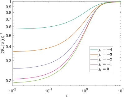
Figure 1: The absolute square of the overlap $\langle\Psi_{\infty}|\Psi(t)\rangle$ between the asymptotically exact analytical answer $\Psi_{\infty}$ and direct numerical solution $\Psi(t)$ of the nonstationary Schrödinger equation for the BCS Hamiltonian with time-dependent coupling constant $g(t)=\frac{\eta}{Nt}$. The number of energy levels $\varepsilon_{j}=\frac{j}{N}$ is $N=10$, $\eta=1$, and $\jmath_{z}$ is the $z$-component of the total spin ($2\jmath_{z}+N$ is the total number of fermions). Here and in all remaining figures we start the evolution from the ground state at $t=0^{+}$, but set the initial value of $t$ in the Hamiltonian to $t_{0}$. By default $t_{0}=10^{-5}$ in all figures. We see that $|\langle\Psi_{\infty}|\Psi(t)\rangle|\to 1$ at large $t$ confirming the exact answer (42).

We double check our result numerically by evaluating the absolute square of the overlap, $|\langle\Psi_{\infty}|\Psi(t)\rangle|^{2}$, where we compute $\Psi_{\infty}$ using Eq. (42) and $\Psi(t)$ via a direct numerical simulation of the nonstationary Schrödinger equation. If Eq. (42) is valid, we must have $|\langle\Psi_{\infty}|\Psi(t)\rangle|^{2}\to 1$ as $t\to+\infty$, which is what we indeed observe in Fig. 1. See also Figs. 3 and 4 for further confirmation of Eq. (42).

V.1 Observables

We first use the late-time wave function (42) to evaluate several basic observables for finite $N$ before turning our attention to the thermodynamic limit of general $n$-point equal time correlation functions in Sec. VII. We also compare these asymptotically exact finite $N$ results with direct numerical simulations and mean-field answers.

Easiest to write is the probability distribution $P(\{s^{z}\})$ of finding the configuration $\lvert\{s^{z}\}\rangle=\lvert s_{1}^{z}s_{2}^{z}\ldots\rangle$. This distribution does not depend on the phases $\theta_{\alpha}$ and $\Lambda_{\{\alpha\}}$ and therefore is independent of $\varepsilon_{j}$ and insensitive to the entanglement due to $\Lambda_{\{\alpha\}}$. In fact, $P(\{s^{z}\})$ has already been found in Ref. 36 via a different approach [58], namely, by exploiting commuting multi-time Hamiltonian flows. In time-dependent integrability, such commuting flows play a role similar to integrals of motion for autonomous quantum integrable systems [58, 52, 57]. We observe from Eq. (42) that the ratio of the probability of the spin at $\varepsilon_{\alpha}$ being up to the probability of it being down is $e^{\frac{-2\pi\alpha}{\nu}}$. Equivalently, we can say that the probabilities of $s_{\alpha}^{z}=\pm\frac{1}{2}$ are proportional to $e^{\frac{-2\pi\alpha s_{\alpha}^{z}}{\nu}}$ and therefore

$$P(\{s^{z}\})=Z^{-1}e^{-\frac{2\pi}{\nu}\sum_{k}ks_{k}^{z}}\delta\Bigl{[}{\textstyle\sum_{k}\!s_{k}^{z}},\jmath_{z}\Bigr{]},$$ (44)

where $\jmath_{z}$ is the $z$-component of the total spin as before, $\delta[a,b]\equiv\delta_{ab}$ is the Kronecker delta, and $Z^{-1}$ is the normalization constant. The independence of $P(\{s^{z}\})$ from the distribution of the single-particle energies $\varepsilon_{j}$ is a distinguishing characteristic of time-dependent integrability [58]. We confirm this in Fig. 2 where we plot the late-time $\langle\hat{s}_{j}^{z}\rangle$ as a function of $j$ for $g(t)\propto t^{-a}$ with $a=0.9$ and $a=1$. Notice that $\langle\hat{s}_{j}^{z}\rangle$ does not change with the distribution of $\varepsilon_{j}$ for $a=1$ and does for $a=0.9$.

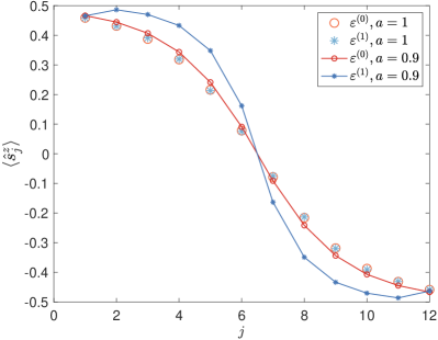
Figure 2: The effect of breaking the time-dependent integrability. Here we compare $\langle\hat{s}_{j}^{z}\rangle$ (equivalent to fermion occupation numbers) at $t\to+\infty$ for two single-particle level distributions and different $g(t)$. The system evolves with the quantum BCS Hamiltonian with coupling $g(t)\propto\frac{\eta}{t^{a}}$ starting from the ground state at $t=0^{+}$. The number of levels and fermions is $N=12$, $\eta=1$, and the two level distributions are: $\varepsilon^{(0)}_{j}=\frac{j}{N}$ and $\varepsilon^{(1)}_{j}=0.49+0.002j$ for all $j\neq 1$ and $\varepsilon^{(1)}_{1}=0.1$. The case $a=1$ is integrable and we see that $\langle\hat{s}_{j}^{z}\rangle$ does not depend on the level distribution (unlike for $a=0.9$), which is characteristic of time-dependent integrability.

The expectation value of the $z$-component of a spin in the state $\Psi_{\infty}$ is

$$\langle\hat{s}_{j}^{z}\rangle_{\Psi_{\infty}}=C_{\infty}\sum_{\{\alpha\}}\left[I_{\{\alpha\}}(j)-\frac{1}{2}\right]\prod_{\alpha}e^{-\frac{2\pi\alpha}{\nu}},$$ (45)

where the indicator function $I_{\{\alpha\}}(j)$ is 1 if $j$ belongs to the set $\{\alpha\}$ and zero otherwise, and $C_{\infty}$ is the inverse norm of the late-time wave function squared,

$$\frac{1}{C_{\infty}}=\sum_{\left\{\alpha\right\}}\prod_{\alpha}e^{{-\frac{2\pi\alpha}{\nu}}}.$$ (46)

Similarly, we evaluate the correlation function

$$\langle\hat{s}_{k}^{+}\hat{s}_{j}^{-}\rangle_{\Psi_{\infty}}=C_{\infty}e^{-2it(\epsilon_{j}-\epsilon_{k})}e^{-\frac{\pi(j+k)}{\nu}}\prod_{q\neq j,k}\biggr{\lvert}\frac{\epsilon_{q}-\epsilon_{j}}{\epsilon_{q}-\epsilon_{k}}\biggr{\rvert}^{-\frac{i}{\nu}}$$

$$\times\sum_{\begin{subarray}{c}\left\{\beta\right\}\\ \beta\neq j,k\end{subarray}}\prod_{\beta}e^{-\frac{2\pi\beta}{\nu}}\biggr{\lvert}\frac{\epsilon_{\beta}-\epsilon_{j}}{\epsilon_{\beta}-\epsilon_{k}}\biggr{\rvert}^{\frac{2i}{\nu}}.$$ (47)

Here, the set $\{\beta\}$ corresponds to all configurations with $N_{\uparrow}-1$ up spins. Importantly, the correlation function $\langle\hat{s}_{k}^{+}\hat{s}_{j}^{-}\rangle$ depends on $\varepsilon_{j}$, unlike $\langle\hat{s}_{j}^{z}\rangle$ and $P(\{s^{z}\})$. In Figs. 3 and 4 we compare Eqs. (45) and (47) with direct numerical simulations of the nonstationary Schrödinger equation and the corresponding late-time dynamical variables in the BCS mean-field (classical) dynamics that we obtain in the next section.

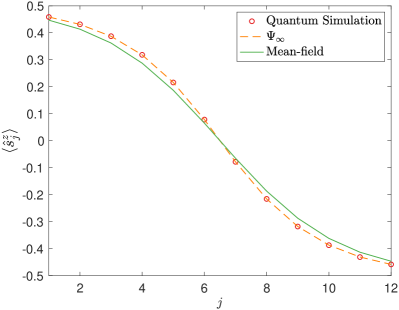
Figure 3: Comparison of three answers for the late-time distribution of $\langle\hat{s}_{j}^{z}\rangle$ for the time-dependent quantum BCS Hamiltonian for $N=12$ energy levels $\varepsilon_{j}$ and 6 fermion pairs. Other parameters are as in Fig. 1. One answer is from a direct numerical simulation of the quantum dynamics. The other is the average $\langle\hat{s}_{j}^{z}\rangle_{\Psi_{\infty}}$ evaluated using the exact analytical late-time wave function $\Psi_{\infty}$ in Eq. (42). These two answers are indistinguishable. The third is the exact analytical answer for the mean-field dynamics in the thermodynamic limit.

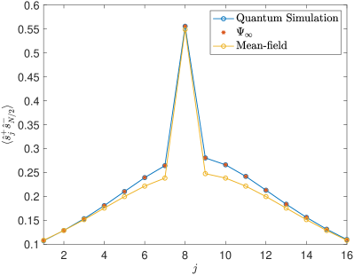
Figure 4: Same as Fig. 3 but for the average $\langle\hat{s}^{+}_{j}\hat{s}^{-}_{N/2}\rangle$ for $N=16$ levels and eight fermion pairs. To evaluate the same-level value $\langle\hat{s}^{+}_{N/2}\hat{s}^{-}_{N/2}\rangle$, we use the spin-$1/2$ identity $\langle\hat{s}^{+}_{N/2}\hat{s}^{-}_{N/2}\rangle=1/2+\langle\hat{s}_{N/2}^{z}\rangle$ as explained below Eq. (55).

VI Exact classical BCS dynamics

We saw above that in the BCS mean-field approximation the averages $\bm{S}_{k}=\langle\hat{\bm{s}}_{k}\rangle$ evolve according to Hamilton’s equations of motion for the classical counterpart of the BCS Hamiltonian,

$$H(t)=\sum_{j=1}^{N}2\varepsilon_{j}S_{j}^{z}-\frac{\eta}{Nt}\sum_{j,k=1}^{N}S_{j}^{+}S_{k}^{-},$$ (48)

with standard angular momentum Poisson brackets for components of $\bm{S}_{j}$. Launched from a BCS product state, the mean-field time evolution keeps the system in a product state at all times, the length of vectors $\bm{S}_{j}$ is $S=\frac{1}{2}$, and knowing $\langle\hat{\bm{s}}_{j}\rangle$ at time $t$, we also know the corresponding BCS product wave function up to a global phase.

Here we present the exact solution for the long time dynamics of the classical Hamiltonian (48). We derive this from the formal solution of Sec. IV by taking the classical limit, where $\hbar\to 0$ and the magnitude of quantum spins $s\to\infty$ in the generalized BCS Hamiltonian (13) so that $\hbar s=S=\frac{1}{2}$. Before the classical limit, we take the long time limit where the multivariable contour integral (33) localizes to its stationary points. Our treatment is similar to that in Sec. V but now solutions of the stationary point equations are highly degenerate and as a result the calculations are more complicated.

We relegate the details of the derivation to Appendix A and just state the answer here: the $t\to+\infty$ asymptote of classical spins $\bm{S}_{j}$ for $N\to\infty$ is

$$S_{j}^{-}=\frac{e^{-2i\varepsilon_{j}t+i\varphi_{j}}}{2\cosh\zeta_{j}},\quad S_{j}^{z}=-\frac{1}{2}\tanh\zeta_{j},$$ (49a)

$$\varphi_{j}=-\frac{\eta}{N}\sum_{k\neq j}\tanh\zeta_{k}\ln|\varepsilon_{k}-\varepsilon_{j}|,$$ (49b)

$$\zeta_{j}=\frac{\pi\eta(j-\mu)}{N},$$ (49c)

where $\mu$ is a Lagrange multiplier (chemical potential) given by Eq. (51) below. We check the analytical results (49) against direct numerical simulation of Hamilton’s (mean-field) equations of motion (18) for $N=10^{3}$ and $N=20$ classical spins in Figs. 5 and 6 and find excellent agreement.

The chemical potential $\mu$ is set by the condition that the conserved $z$-component of the total spin $\bm{J}$ be equal to its initial value,

$$J_{z}=\sum_{k=1}^{N}S_{k}^{z}=-\frac{1}{2}\sum_{k=1}^{N}\tanh\left[\frac{\pi\eta(k-\mu)}{N}\right].$$ (50)

In the thermodynamic limit $N\to\infty$, the sum turns into an integral. Integrating and solving for $\mu$, we find

$$\mu=\frac{N+1}{2}+\frac{N}{2\pi\eta}\ln\left\{\frac{\sinh\left[\pi\eta\left(\frac{1}{2}+\frac{J_{z}}{N}\right)\right]}{\sinh\left[\pi\eta\left(\frac{1}{2}-\frac{J_{z}}{N}\right)\right]}\right\}.$$ (51)

We kept the subleading correction ($N+1$ instead of simply $N$ in the first term on the r.h.s.) because it reproduces $\mu=\frac{N+1}{2}$ for $J_{z}=0$ which is exact for any even $N$ and significantly improves the agreement with finite $N$ numerics.

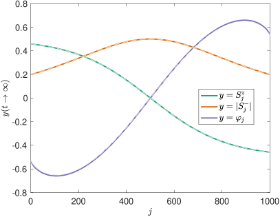
Figure 5: Classical (mean-field) dynamics of the BCS Hamiltonian with coupling $g(t)\propto\frac{\eta}{t}$ asymptotes to a state $S_{j}^{z}=\text{const}$ and $S_{j}^{-}=|S_{j}^{-}|e^{-2i\varepsilon_{j}t}e^{i\varphi_{j}}$ at late times. In the text, we derived exact analytic expressions for $S_{j}^{z}$, $|S_{j}^{-}|$, and $\varphi_{j}$ in the limit $N\to\infty$ [dashed curves, see Eq. (49)]. Here we compare them with direct numerical simulation of the mean-field equations of motion [solid curves] for $N=10^{3}$ classical spins $\bm{S}_{j}$ and $z$-component of the total spin $J_{z}=0$. Maximum relative errors for $S_{j}^{z}$, $|S_{j}^{-}|$, and $\varphi_{j}$ are $0.1\%,0.4\%$, and $2\%$, respectively. Other parameters are as in Fig. 1.

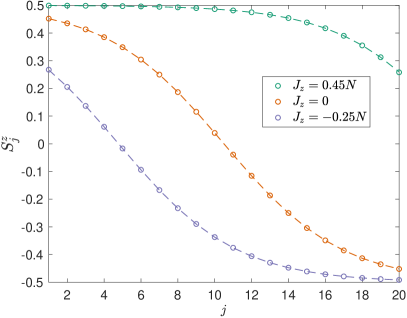
Figure 6: Comparison of our analytic answer (dashed curves) for $S_{j}^{z}=\langle\hat{s}_{j}^{z}\rangle$ in the late-time asymptotic state of the mean-field BCS dynamics with coupling $g(t)\propto\frac{\eta}{t}$ and direct numerical simulations (circles) of the equations of motion for $N=20$ classical spins and three different values of $J_{z}=\sum_{k}S_{k}^{z}$. The significance of $S_{j}^{z}$ is in its relation to the average fermion occupation number for level $\varepsilon_{j}$, $\langle\hat{n}_{j}\rangle=2S_{j}^{z}+1$. Other parameters are the same as in Fig. 1. Note how close our $N\to\infty$ answer is to the results of simulations with only 20 spins. This is consistent with our numerical observation in Sec. XI that the corrections to this limit within mean-field scale as $N^{-\frac{3}{2}}$ rather than $N^{-1}$.

Within the mean-field treatment, each quantum spin $\hat{\bm{s}}_{j}$ evolves individually in an effective magnetic field $2(\varepsilon_{j}\bm{z}-\bm{\Delta})$. The wave function of the system is thus of the BCS product form

$$\Psi_{\mathrm{mf}}=\prod_{k=1}^{N}\left(u_{k}|\!\downarrow\rangle+v_{k}|\!\uparrow\rangle\right).$$ (52)

at all times provided it was of this form at $t=0$. Normalization requires $|u_{k}|^{2}+|v_{k}|^{2}=1$ and Eqs. (52) and (49) together with $\bm{S}_{k}=\langle\hat{\bm{s}}_{k}\rangle$ imply

$$\langle\hat{s}_{k}^{+}\rangle_{\mathrm{mf}}=u_{k}v_{k}^{*}=\frac{e^{2i\varepsilon_{k}t}e^{-i\varphi_{k}}}{2\cosh\zeta_{k}},$$ (53a)

$$\langle\hat{s}_{k}^{-}\rangle_{\mathrm{mf}}=u_{k}^{*}v_{k}=\frac{e^{-2i\varepsilon_{k}t}e^{i\varphi_{k}}}{2\cosh\zeta_{k}},$$ (53b)

$$\langle\hat{s}_{k}^{z}\rangle_{\mathrm{mf}}=\frac{|v_{k}|^{2}-|u_{k}|^{2}}{2}=-\frac{1}{2}\tanh\zeta_{k}.$$ (53c)

The subscript “mf” indicates the expectation values in the late-time mean-field wave function (52). Using these equations, we reconstruct the Bogoliubov amplitudes

$$u_{k}=\frac{e^{\frac{\zeta_{k}-i\varphi_{k}}{2}}}{\sqrt{2\cosh\zeta_{k}}},\quad v_{k}=\frac{e^{-2i\varepsilon_{k}t}e^{\frac{-\zeta_{k}+i\varphi_{k}}{2}}}{\sqrt{2\cosh\zeta_{k}}},$$ (54)

up to a common phase which only affects the global phase of $\Psi_{\mathrm{mf}}$. Equations (52) and (54) provide the exact late-time mean-field wave function for the time evolution with the BCS Hamiltonian with interaction strength inversely proportional to time starting from the mean-field ground state at $t=0^{+}$ in the thermodynamic limit.

Due to the product form of the mean-field wave function, it is simple to determine the expectation value of an arbitrary product of spin operators

$$\biggl{\langle}\prod_{m=1}^{n}\hat{s}_{j_{m}}^{r_{m}}\biggr{\rangle}_{\mathrm{mf}}=\prod_{k=1}^{n}\bigl{\langle}\hat{s}_{j_{m}}^{r_{m}}\bigr{\rangle}_{\mathrm{mf}},$$ (55)

where the upper indices $r_{m}$ take values $+,-$, or $z$ and individual spin averages $\bigl{\langle}\hat{s}_{j_{m}}^{r_{m}}\bigr{\rangle}_{\mathrm{mf}}$ are given by Eq. (53). It is understood that there is only one spin operator per energy level $\varepsilon_{j}$ in Eq. (55). In other words, any operator nonlinear in the components of $\bm{s}_{j}$ must be reduced to a linear one before comparing the averages. This can always be done for spin-$\frac{1}{2}$, e.g., $\hat{s}_{j}^{+}\hat{s}_{j}^{-}=\frac{1}{2}+\hat{s}_{j}^{z}$, $(\hat{s}_{j}^{z})^{2}=\frac{1}{4}$, etc. Otherwise, Eq. (55) may not hold because, for example, $\langle(\hat{s}_{j}^{z})^{2}\rangle_{\mathrm{mf}}=\frac{1}{4}\neq(\langle\hat{s}_{j}^{z}\rangle_{\mathrm{mf}})^{2}$.

VII Thermodynamic limit of quantum dynamics

In this section, we show how a BCS product state emerges in the thermodynamic limit from the entangled finite $N$ wave function $\Psi_{\infty}$ – the late-time asymptotic solution (42) of the nonstationary Schrödinger equation for the quantum BCS Hamiltonian (11) with interaction strength inversely proportional to time. The precise statement is that any local equal time correlation function of fermionic or spin operators evaluated in the exact asymptotic state $\Psi_{\infty}$ is identical to that in the product state $\Psi_{\mathrm{mf}}$ of the mean-field (classical) dynamics in this limit. Recall that we say a quantity is local if the number $n$ of single-particle levels $\varepsilon_{k}$ (“points”) it involves is such that $\frac{n}{N}\to 0$ when $N\to\infty$ [59]. All correlators of this type will be straightforward to evaluate once we establish this correspondence between quantum and classical dynamics.

However, $\Psi_{\infty}\neq\Psi_{\mathrm{mf}}$ even in the thermodynamic limit. This manifests itself in non-local quantities involving an infinite number of points in the thermodynamic limit, such as, e.g., $\langle\hat{s}_{1}^{-}\dots\hat{s}_{N_{\uparrow}}^{-}s_{N_{\uparrow}+1}^{+}\dots\hat{s}_{2N_{\uparrow}}^{+}\rangle$, where $N_{\uparrow}$ is the number of up spins, or the von Neumann entanglement entropy. The values of quantities of this type are generally different for $\Psi_{\infty}$ and $\Psi_{\mathrm{mf}}$. This is not specific to the nonautonomous setup as these quantities similarly disagree between the exact and BCS ground states for the time-independent BCS Hamiltonian. An even more interesting example of the breakdown of the classical picture for global observables is the Loschmidt echo [39]. Within mean-field approach we obtain the classical Loschmidt echo, i.e., the echo of the classical spin Hamiltonian (15), which is qualitatively different from the true quantum echo, see Ref. 39 for further details.

The crucial step in deriving the thermodynamic limit of the late-time quantum dynamics is to notice by inspecting Eqs. (40) and (41) that we can write $\Psi_{\infty}$ in the form of a generalized projected BCS state [cf. Eq. (23)]

$$\Psi_{\infty}=P_{N_{\uparrow}}\prod_{k=1}^{N}\left(\hat{U}_{k}|\!\downarrow\rangle+\hat{V}_{k}|\!\uparrow\rangle\right),$$ (56)

where $P_{N_{\uparrow}}$ is the projector onto the subspace with $N_{\uparrow}$ up spins and

$$\hat{U}_{k}=e^{-\frac{i\hat{\varphi}_{k}}{2}},\quad\hat{V}_{k}=e^{\frac{i\hat{\varphi}_{k}}{2}-2i\varepsilon_{k}t-\frac{\pi k}{\nu}},$$ (57a)

$$\hat{\varphi}_{k}=\frac{2}{\nu}\sum_{j\neq k}\hat{s}_{j}^{z}\ln|\varepsilon_{j}-\varepsilon_{k}|.$$ (57b)

It is understood that when the product (56) is expanded, all ket vectors are placed to the right of the operators $e^{\mp\frac{i\hat{\varphi}_{k}}{2}}$. The projector ensures that we end up with the summation over the same basis states $|\{\alpha\}\rangle$ with $N_{\uparrow}$ up spins as in Eq. (41). The terms $-2i\varepsilon_{k}t-\frac{\pi k}{\nu}$ then add up to the first two sums in Eq. (40) multiplied by $-\frac{i}{\nu}$. Similarly, $\hat{\varphi}_{k}$ correspond to the last sum in Eq. (40). States $|\!\downarrow\rangle$ and $|\!\uparrow\rangle$ come with $e^{\mp i\frac{\hat{\varphi}_{k}}{2}}$ in Eq. (56) because for them $\hat{s}_{k}^{z}\to\mp\frac{1}{2}$ in Eq. (40).

VII.1 Local operators

First, we study local operators in the thermodynamic limit. As usual in the theory of superconductivity, we understand the thermodynamic limit as $N\to\infty$ so that the single-particle levels $\varepsilon_{j}$ fill a finite energy interval with a piecewise continuous density of states and the number of fermions per level $\frac{N_{\mathrm{f}}}{N}=\frac{2N_{\uparrow}}{N}$ stays finite. The latter condition is equivalent to a finite density of fermions.

We start with $\langle\hat{s}_{k}^{+}\hat{s}_{j}^{-}\rangle_{\Psi_{\infty}}$ for $j\neq k$ and then generalize to arbitrary products. It is helpful to rewrite Eq. (56) as an integral [cf. Eq. (24)]

$$\Psi_{\infty}=\frac{1}{2\pi}\int_{0}^{2\pi}\!\!\!\!\!d\phi e^{i\phi N_{\uparrow}}\prod_{k}\left(\hat{U}_{k}|\!\downarrow\rangle+e^{-i\phi}\hat{V}_{k}|\!\uparrow\rangle\right).$$ (58)

Consider $\langle\Psi_{\infty}|\Psi_{\infty}\rangle$. This is a double integral over $\phi$ and $\phi^{\prime}$. The integrand depends only on $\xi=\phi-\phi^{\prime}$, so one integration simply gives $2\pi$. Taking this overlap converts $\hat{s}_{j}^{z}\to\langle\hat{s}_{j}^{z}\rangle_{\Psi_{\infty}}$ because $e^{c\hat{s}_{z}}$ is linear in $\hat{s}_{z}$ for spin-$\frac{1}{2}$ and $\hat{s}_{j}^{z}$ mutually commute. We find

$$\langle\Psi_{\infty}|\Psi_{\infty}\rangle=\frac{1}{2\pi}\int_{-2\pi}^{2\pi}d\xi e^{G(\xi)},$$ (59)

where

$$G(\xi)=i\xi N_{\uparrow}+\sum_{k}\ln\left(|U_{k}|^{2}+e^{-i\xi}|V_{k}|^{2}\right),$$ (60)

and

$$U_{k}=e^{-\frac{i\varphi_{k}}{2}},\quad V_{k}=e^{\frac{i\varphi_{k}}{2}-2i\varepsilon_{k}t-\frac{\pi k}{\nu}},$$ (61a)

$$\varphi_{k}=\frac{2}{\nu}\sum_{j\neq k}\langle\hat{s}_{j}^{z}\rangle_{\Psi_{\infty}}\ln|\varepsilon_{j}-\varepsilon_{k}|.$$ (61b)

Similarly, we can evaluate various matrix elements. Take, for example, $\langle\Psi_{\infty}|\hat{s}_{k}^{+}\hat{s}_{j}^{-}|{\Psi_{\infty}}\rangle$. Here it is important to realize that operators $\hat{s}_{k}^{+}$ and $\hat{s}_{j}^{-}$ commute with $\hat{U}_{l}$ and $\hat{V}_{l}$ up to terms of order $\frac{1}{N}$. Keeping this in mind, we go through the same steps as for $\langle\Psi_{\infty}|\Psi_{\infty}\rangle$ and obtain

$$\begin{split}\langle\Psi_{\infty}|&\hat{s}_{k}^{+}\hat{s}_{j}^{-}|{\Psi_{\infty}}\rangle=\\ =&\frac{1}{2\pi}\!\!\!\int\limits_{-2\pi}^{2\pi}\frac{U_{k}V_{k}^{*}U_{j}^{*}V_{j}e^{-i\xi}e^{G(\xi)}d\xi}{\left(|U_{k}|^{2}+e^{-i\xi}|V_{k}|^{2}\right)\left(|U_{j}|^{2}+e^{-i\xi}|V_{j}|^{2}\right)}.\end{split}$$ (62)

The additional factors in this equation as compared to Eq. (59) result from the action of $\hat{s}_{j}^{-}$ on the state $U_{j}|\!\downarrow\rangle+e^{-i\phi}V_{j}|\!\uparrow\rangle$ and the analogous action of $\hat{s}_{k}^{+}$. Eq. (62) is only valid when $j\neq k$ and only up to terms of order $\frac{1}{N}$.

Integrals of the form (59) and (62) have been analyzed extensively in studies of the equilibrium projected BCS wave function and its equivalence to the regular BCS product state in the thermodynamic limit [71, 72]. It is known that the saddle point method becomes exact in the thermodynamic limit because $G(\xi)$ is of order $N$. For the same reason, the saddle point $\xi_{0}$ is the same for both integrals (59) and (62). Evaluating the integrals with this method, we find that $\langle\hat{s}_{k}^{+}\hat{s}_{j}^{-}\rangle_{\Psi_{\infty}}$ is identical to the average of the same operator $\hat{s}_{k}^{+}\hat{s}_{j}^{-}$ in a product state

$$\Psi_{\mathrm{thd}}=C_{\mathrm{n}}\prod_{k=1}^{N}\left(U_{k}|\!\downarrow\rangle+e^{\frac{\pi\mu}{\nu}}V_{k}|\!\uparrow\rangle\right),$$ (63)

where $\mu=-\frac{i\nu\xi_{0}}{\pi}$ and $C_{\mathrm{n}}$ is a normalization constant. The subscript “thd” stands for “thermodynamic” indicating that this wave function is exact for evaluating certain correlation functions in the thermodynamic limit. Evaluating $C_{\mathrm{n}}$ and recalling that $\nu=\frac{\eta}{N}$ [see Eq. (12)], we see that $\Psi_{\mathrm{thd}}$ is identical to the late-time mean-field wave function (52),

$$\Psi_{\mathrm{thd}}=\Psi_{\mathrm{mf}}=\prod_{k=1}^{N}\left(u_{k}|\!\downarrow\rangle+v_{k}|\!\uparrow\rangle\right),$$ (64)

where $u_{k}$ and $v_{k}$ are given by Eq. (54).

There is nothing special about $\hat{s}_{k}^{+}\hat{s}_{j}^{-}$. The same logic applies to general products of $\hat{s}^{+},\hat{s}^{-},$ and $\hat{s}^{z}$,

$$\hat{O}=\prod_{m=1}^{n}\hat{s}_{j_{m}}^{r_{m}},$$ (65)

where $r_{m}=+,-$, or $z$ and as before there is no more than one spin operator for each $j_{m}$. The number of operators $n$ must be such that $\frac{n}{N}\to 0$ when $N\to\infty$, i.e. $\hat{O}$ must be local. Otherwise, terms of the order $N^{-1}$ of the type we neglected in deriving Eq. (63) can add up to a contribution of order one. Nonzero matrix elements of $\hat{O}$ between states $\Psi_{\infty}(N_{\uparrow}+\Delta N_{\uparrow})$ and $\Psi_{\infty}(N_{\uparrow})$ coincide with its expectation value in the product state (52) in the thermodynamic limit ($\Delta N_{\uparrow}$ is the number of $\hat{s}^{+}$ minus number of $\hat{s}^{-}$ in $\hat{O}$, i.e., the amount by which it increases the number of up spins). Therefore, using Eq. (55) we have to the leading order in $\frac{n}{N}$,

$$\Bigl{\langle}\widetilde{N}_{\uparrow}\Bigl{|}\prod_{m=1}^{n}\hat{s}_{j_{m}}^{r_{m}}\Bigr{|}N_{\uparrow}\Bigr{\rangle}_{\infty}=\prod_{k=1}^{n}\bigl{\langle}\hat{s}_{j_{m}}^{r_{m}}\bigr{\rangle}_{\mathrm{mf}}.$$ (66)

Here $|N_{\uparrow}\rangle_{\infty}$ is the normalized version of $\Psi_{\infty}(N_{\uparrow})$,

$$|N_{\uparrow}\rangle_{\infty}=\frac{\Psi_{\infty}(N_{\uparrow})}{{\left\lVert\Psi_{\infty}(N_{\uparrow})\right\rVert}},$$ (67)

and $\widetilde{N}_{\uparrow}=N_{\uparrow}+\Delta N_{\uparrow}$. Note also that the matrix elements of arbitrary products of fermionic creation $\hat{c}^{\dagger}_{j\sigma}$ and annihilation $\hat{c}_{k\sigma^{\prime}}$ operators are either zero or reduce to matrix elements of the form (66).

The quantity $\mu$ in Eq. (63) is determined by the equation $N_{\uparrow}-\frac{N}{2}=\jmath_{z}=\sum_{k=1}^{N}\langle\hat{s}_{k}^{z}\rangle_{\mathrm{mf}}$, which is a consequence of the conservation of the $z$-projection of the total spin $\hat{\bm{\jmath}}$. Simultaneously it is the equation for the stationary point $\xi_{0}$ of $G(\xi)$ defined in Eq. (60) as it should be because we defined $\mu$ in this section as $\mu=-\frac{i\nu\xi_{0}}{\pi}$. Since $J_{z}=\langle\hat{\jmath}_{z}\rangle=\jmath_{z}$ and $S_{k}^{z}=\langle\hat{s}_{k}^{z}\rangle_{\mathrm{mf}}$, this equation is equivalent to Eq. (50) and $\mu$ in Eq. (63) is therefore the same as the chemical potential (51) of the mean-field dynamics.

Equations (66, 53, 49b), and (49c) determine explicitly the exact thermodynamic limit of any matrix element on the left hand side of Eq. (66). In particular,

$$\langle\hat{s}_{k}^{+}\hat{s}_{j}^{-}\rangle_{\Psi_{\infty}}=\frac{e^{2i(\varepsilon_{k}-\varepsilon_{j})t}e^{i(\varphi_{j}-\varphi_{k})}}{2\cosh\zeta_{k}\cosh\zeta_{j}},\quad j\neq k,$$ (68a)

$$\langle\hat{s}_{k}^{+}\hat{s}_{k}^{-}\rangle_{\Psi_{\infty}}=\frac{1}{2}-\frac{1}{2}\tanh\zeta_{k},$$ (68b)

$$\langle\hat{s}_{k}^{z}\rangle_{\Psi_{\infty}}=-\frac{1}{2}\tanh\zeta_{k}.$$ (68c)

$$\langle N_{\uparrow}-1|\hat{s}_{k}^{-}|N_{\uparrow}\rangle_{\infty}=\frac{e^{-2i\varepsilon_{k}t}e^{i\varphi_{k}}}{2\cosh\zeta_{k}}.$$ (68d)

Note that $\langle\dots\rangle_{\Psi_{\infty}}\equiv\langle N_{\uparrow}|\dots|N_{\uparrow}\rangle_{\infty}$. As a check on our results, we also derived the thermodynamic limit of $\langle\hat{s}_{k}^{z}\rangle_{\Psi_{\infty}}$ and $\langle\hat{s}_{k}^{+}\hat{s}_{j}^{-}\rangle_{\Psi_{\infty}}$ directly from Eqs. (45) and (47) by writing them as integrals and using the saddle point method, which is exact in this limit. The answers are precisely Eqs. (68c) and (68a). Instead of the BCS-like product $\Psi_{\mathrm{mf}}$ we can equally well employ the projected version of this state

$$\Psi_{\mathrm{pmf}}=P_{N_{\uparrow}}\Psi_{\mathrm{mf}}=P_{N_{\uparrow}}\prod_{k=1}^{N}\left(u_{k}|\!\downarrow\rangle+v_{k}|\!\uparrow\rangle\right).$$ (69)

We see this in the same way as we showed the equivalence of $\Psi_{\mathrm{mf}}$ and $\Psi_{\infty}$ only without the complication of $\hat{U}_{k}$ and $\hat{V}_{k}$ being operators, see also Refs. 71, 72.

We conclude that the thermodynamic limits of averages of local operators $\hat{O}$ in the late-time asymptotic state of the exact quantum BCS dynamics and in the late-time asymptotic state of mean-field (classical) BCS dynamics coincide exactly . Let us emphasize once more that when $\hat{O}$ does not conserve the total fermion number, we define its average in the asymptotic solution of quantum dynamics with definite fermion number as the nonzero matrix element between solutions with different fermion numbers. Its expectation value in the state $\Psi_{\infty}$ is zero and not useful for comparison to mean field. When $\hat{O}$ commutes with $N_{\mathrm{f}}$, its average and expectation value in any state are the same.

Note that local correlators are the ones most readily accessible in experiment. In this sense, BCS mean field is exact far from equilibrium for the evolution launched from the exact quantum ground state with a definitive number of fermions. This is true despite the fact that the BCS order parameter vanishes at late times, see the discussion below Eq. (22). However, the status of mean-field changes when: (1) the initial state of the quantum BCS evolution is not a particle number eigenstate and $\hat{O}$ does not commute with the total fermion number operator or (2) for non-local quantiles, as we will see shortly.

VII.2 Entanglement entropy and other non-local quantities

Even though matrix elements of local operators in the exact late-time state $\Psi_{\infty}$ of quantum time evolution from the exact ground state and in the BCS product state $\Psi_{\mathrm{mf}}$ of the mean-field (classical) evolution as well as in the projected BCS state $\Psi_{\mathrm{pmf}}$ are identical in the thermodynamic limit, $\Psi_{\infty}\neq\Psi_{\mathrm{mf}}$ and $\Psi_{\infty}\neq\Psi_{\mathrm{pmf}}$. We see this by comparing coefficients at basis states in Eqs. (69) and (42). The von Neumann entanglement entropy $\mathtt{S}_{\mathrm{ent}}$ is zero for $\Psi_{\mathrm{mf}}$ and of order $\ln N$ for both $\Psi_{\infty}$ and $\Psi_{\mathrm{pmf}}$, as we will see below. Moreover, we observe numerically that $\mathtt{S}_{\mathrm{ent}}(\Psi_{\mathrm{pmf}})\approx\mathtt{S}_{\mathrm{ent}}(\Psi_{\infty})$.

It is not difficult to write an operator whose quantum average is different in $\Psi_{\infty}$ and in $\Psi_{\mathrm{mf}}$ or $\Psi_{\mathrm{pmf}}$. The number of spins involved in such an operator is necessarily proportional to $N$ in the thermodynamic limit. Consider, for example, operators $|\bm{e}_{2}\rangle\langle\bm{e}_{1}|$ that convert a basis state $|\bm{e}_{1}\rangle$ into a basis state $|\bm{e}_{2}\rangle$. One of these operators is

$$\hat{s}_{1}^{-}\dots\hat{s}_{N_{\uparrow}}^{-}s_{N_{\uparrow}+1}^{+}\dots\hat{s}_{2N_{\uparrow}}^{+}.$$ (70)

Evaluating its expectation value in the state $\Psi_{\infty}$ using Eq. (41) or Eq. (42) and in the state $\Psi_{\mathrm{mf}}$ (or equivalently in $\Psi_{\mathrm{pmf}}$) using Eqs. (52) or (54), we see that they generally do not agree even in the thermodynamic limit $N\to\infty$ keeping $\frac{N_{\mathrm{f}}}{N}=\frac{2N_{\uparrow}}{N}$ constant.

A popular example of a non-local quantity is the bipartite von Neumann entanglement entropy

$$\mathtt{S}_{\mathrm{ent}}=-\mathrm{Tr}\,[\rho_{A}\ln\rho_{A}],$$ (71)

where $\rho_{A}=\mathrm{Tr}\,_{\!\!\bar{A}}\,\rho$ is the reduced density matrix of the subsystem $A$: the trace of the system density matrix over the complement of $A$. Suppose $N$ is even and consider the most interesting case $N_{\uparrow}=\frac{N}{2}$. Our choice of $A$ is the spins $\hat{\bm{s}}_{j}$ corresponding to the bottom half of the energies $\varepsilon_{j}$. We find that the entanglement entropy for the nonautonomous quantum BCS dynamics plateaus at late times and for large $N$ at

$$\mathtt{S}_{\mathrm{ent}}=c(\eta)\ln N,$$ (72)

where $c(\eta)$ is a function of $\eta$ of order one. This formula holds for both initial conditions we analyzed: the exact and the BCS ground states at $t=0^{+}$. We consider the latter initial condition in Sec. XII.1. The asymptotic state of the quantum dynamics launched from the exact ground state at $t=0^{+}$ is $\Psi_{\infty}$. We plot $\mathtt{S}_{\mathrm{ent}}$ versus $\ln N$ for $\Psi_{\infty}$ for a range of $N$ and $\eta=1$ in Fig. 7. A linear fit to this plot gives $c(\eta=1)=0.441$. Remarkably, the entanglement entropy of the projected mean-field state $\Psi_{\mathrm{pmf}}$ closely matches that of the exact asymptotic state $\Psi_{\infty}$.

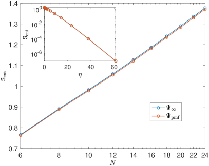
Figure 7: Entanglement entropies $\mathtt{S}_{\mathrm{ent}}$ for the states $\Psi_{\infty}$ and $\Psi_{\mathrm{pmf}}$ vs. $\ln N$, where $N$ is the number of the energy levels $\varepsilon_{k}$, $\Psi_{\infty}$ is the exact solution of the nonstationary Schrödinger equation at $t\to+\infty$ for the quantum BCS Hamiltonian with coupling strength $g(t)\propto\frac{\eta}{t}$ starting from the exact ground state at $t=0^{+}$ and $\Psi_{\mathrm{pmf}}$ is the exact solution of the mean-field version of the same problem projected onto a fixed particle number subspace. Here the number of fermion pairs (number of up pseudospins) is $N_{\uparrow}=\frac{N}{2}$, $\eta=1$, and $\varepsilon_{k}=\frac{k}{N}$. Inset: $\mathtt{S}_{\mathrm{ent}}$ for the same two states as functions of $\eta$; the two curves are indistinguishable on this scale. $\mathtt{S}_{\mathrm{ent}}(\Psi_{\mathrm{pmf}})$ and $\mathtt{S}_{\mathrm{ent}}(\Psi_{\infty})$ agree well already for small $N$ and are approximately linear in $\ln N$ with slopes 0.438 and 0.441, respectively. Note also that $\mathtt{S}_{\mathrm{ent}}$ rapidly decreases with $\eta$ consistent with $\mathtt{S}_{\mathrm{ent}}\to 0$ in the adiabatic limit $\eta\to+\infty$.

We do not prove Eq. (72) for $\Psi_{\infty}$ and $\Psi_{\mathrm{pmf}}$ in general but restrict ourselves to the diabatic, $\eta\to 0$, limit. We see from Eqs. (54, 69), and (42) that in this limit $\Psi_{\mathrm{pmf}}=\Psi_{\infty}=\Psi_{0}$, where $\Psi_{0}$ is the exact $t=0^{+}$ ground state given by Eq. (29). To determine the entanglement entropy for $\Psi_{0}$, we employ the Schmidt decomposition $\Psi_{0}=\sum_{i=1}^{m}w_{i}|p_{i}\rangle_{A}\otimes|q_{i}\rangle_{\bar{A}}$, where $|p_{i}\rangle_{A}$ and $|q_{i}\rangle_{\bar{A}}$ are orthonormal vectors in $A$ and $\bar{A}$. The entanglement entropy can be expressed in terms of the coefficients $w_{i}$ as

$$\mathtt{S}_{\mathrm{ent}}=-\sum_{i=1}^{m}|w_{i}|^{2}\ln|w_{i}|^{2}.$$ (73)

We have

$$\Psi_{0}(N_{\uparrow})=\sum_{N_{\uparrow}^{A}=N_{\mathrm{m}}}^{N_{\uparrow}-N_{\mathrm{m}}}\frac{\mbinom{\frac{N}{2}}{N_{\uparrow}^{A}}}{\sqrt{\vphantom{\prod}\smash[b]{\mbinom{N}{N_{\uparrow}}}}}\left|N_{\uparrow}^{A}\right\rangle_{A}\otimes\left|N_{\uparrow}-N_{\uparrow}^{A}\right\rangle_{\bar{A}},$$ (74)

where $N_{\mathrm{m}}=N_{\uparrow}-\min(\frac{N}{2},N_{\uparrow})$ and $|N_{\uparrow}^{A}\rangle_{A}$ is the state of the subsystem $A$ with a definite number $N_{\uparrow}^{A}$ of up spins and symmetric with respect to an arbitrary permutation of spins. In other words, the subsystem $A$ has the maximum total spin $\frac{N}{4}$ and a definite $z$-projection $N_{\uparrow}^{A}-\frac{N}{4}$ of the total spin. Similarly, $|N_{\uparrow}^{\bar{A}}\rangle$ is the state of the subsystem $\bar{A}$ with the maximum total spin and $N_{\uparrow}^{\bar{A}}$ up spins. In our case $N_{\uparrow}=\frac{N}{2}$, but we wrote Eq. (74) for arbitrary $N_{\uparrow}$ for later use.

Reading off $w_{i}$ from this equation and substituting them into Eq. (73), we see that the values of $N_{\uparrow}^{A}$ close to $\frac{N_{\uparrow}}{2}=\frac{N}{4}$ dominate the summation. Now using the following precise asymptotic expression [73] valid for large $N_{1}$ and $\left|N_{2}-\frac{N_{1}}{2}\right|=o(N_{1}^{\frac{2}{3}})$:

$$2^{-N_{1}}\binom{N_{1}}{N_{2}}=\sqrt{\frac{2}{\pi N_{1}}}e^{-2N_{1}x^{2}},\quad x=\frac{N_{2}}{N_{1}}-\frac{1}{2},$$ (75)

and converting the summation in Eq. (73) into an integration, we obtain the leading large $N$ asymptotic behavior of $\mathtt{S}_{\mathrm{ent}}$,

$$\mathtt{S}_{\mathrm{ent}}=\frac{1}{2}\ln N.$$ (76)

Therefore, $\lim_{\eta\to 0}c(\eta)=\frac{1}{2}$. In the opposite (adiabatic) limit $\eta\to+\infty$, the late-time asymptotic state is the ground state of a noninteracting Fermi gas with no entanglement, i.e., $\lim_{\eta\to+\infty}c(\eta)=0$. Generally, we expect $c(\eta)$ in Eq. (73) to decrease monotonically from $\frac{1}{2}$ to 0 as $\eta$ increases from 0 to $+\infty$, see also the inset in Fig. 7.

Entanglement entropy that scales as $\ln N$ (see also the end of Sec. XII.1) is a purely quantum phenomenon that survives the thermodynamic limit. Indeed, the asymptotic state of the mean-field (classical) dynamics is the product state $\Psi_{\mathrm{mf}}$ with zero entanglement, $\mathtt{S}_{\mathrm{ent}}=0$. However, the projected mean-field state $\Psi_{\mathrm{pmf}}$ appears to match $\mathtt{S}_{\mathrm{ent}}$ of the exact $t\to+\infty$ asymptotic state $\Psi_{\infty}$. Note also that $N\propto V$ and $N\propto N_{\mathrm{f}}$, where $V$ is the system volume and $N_{\mathrm{f}}$ is the fermion number. Therefore, we can equally well say that $\mathtt{S}_{\mathrm{ent}}$ scales as $\ln V$ or $\ln N_{\mathrm{f}}$ in the thermodynamic limit.

We see again that the mean-field approximation breaks down for non-local measures, even though it is exact for local observables in the thermodynamic limit even for far from equilibrium dynamics that involves highly excited states. Note that the many-body wave function of the system is itself non-local and therefore cannot be reproduced by mean field precisely. It is important to emphasize that this obvious breakdown of the BCS mean-field theory for global quantities is not in any way specific to the nonautonomous BCS Hamiltonian. For example, we similarly expect the entanglement entropy of the exact ground state of the quantum BCS Hamiltonian (11) to be proportional to $\ln N$ at $N_{\uparrow}=\frac{N}{2}$ etc.

VIII Steady State Properties

Before comparing quantum and mean-field dynamics for initial states that are not particle number eigenstates, let us discuss several physical properties of the steady state. Two main results of this section are: (1) the late-time steady state is a gapless superconductor whose superconducting properties can only be revealed through energy resolved measurements and (2) it conforms to the generalized Gibbs ensemble. The first result holds for a general protocol of turning off the superconducting coupling $g(t)$. The second one is similarly general as long as the mean field remains exact in the thermodynamic limit (we established this above for dynamics with $g(t)\propto\frac{\eta}{t}$ starting in the $t=0^{+}$ ground state, but it is reasonable to assume the scope of validity of mean field is much broader).

Suppose the interaction vanishes at $t\to+\infty$, such as our $g(t)\propto\frac{\eta}{t}$. Then, at long times the system evolves with the noninteracting part of the Hamiltonian,

$$\hat{H}(t\to+\infty)=\hat{H}_{0}=\sum_{j=1}^{N}2\varepsilon_{j}\hat{s}_{j}^{z}.$$ (77)

Regardless of the history, expectation values of spin components at late times are of the form

$$\langle\hat{s}_{k}^{z}\rangle=\ell_{k},\quad\langle\hat{s}_{k}^{-}\rangle=b_{k}e^{-2i\varepsilon_{k}t},$$ (78a)

$$\langle\hat{s}_{k}^{+}s_{j}^{-}\rangle=B_{kj}e^{2i(\varepsilon_{k}-\varepsilon_{j})t}.$$ (78b)

For $\Psi_{\mathrm{mf}}$, we have $B_{kj}=b_{k}^{*}b_{j}$, $b_{k}=e^{i\varphi_{k}}\sqrt{\vphantom{\sum}\smash[b]{\frac{1}{4}-\ell_{k}^{2}}}$, where $\ell_{k}$ and $\varphi_{k}$ are given by Eqs. (53c) and (49b), respectively. In the thermodynamic limit, $\ell_{k}$ and $B_{kj}$ for $\Psi_{\infty}$ are the same as for $\Psi_{\mathrm{mf}}$ but $b_{k}=0$ , since $\Psi_{\infty}$ is an eigenstate of the total fermion number operator. However, the average of $\hat{s}_{k}^{-}$ in the state $\Psi_{\infty}$ [the l.h.s. of Eq. (68d)] is the same as its expectation value in $\Psi_{\mathrm{mf}}$.

The conventionally defined superconducting order parameter is zero in the steady state because it is proportional to the coupling $g=g(t)$, which vanishes as $t\to+\infty$. Consider instead

$$\Delta_{1}=\frac{1}{N}\sum_{k=1}^{N}\langle\hat{s}_{k}^{-}\rangle,\quad\Delta_{2}=\frac{1}{N}\sqrt{\vphantom{\sum}\smash[b]{\sum\nolimits_{k\neq j}}\langle\hat{s}_{k}^{+}s_{j}^{-}\rangle}.$$ (79)

The first of these quantities is the usual BCS order parameter (20) divided by $gN$. The second is useful for the description of off-diagonal long-range order in states with definite particle number [24, 74] as for them $\Delta_{1}=0$. For a BCS-like product state such as $\Psi_{\mathrm{mf}}$, $\Delta_{2}=\Delta_{1}$ in the thermodynamic limit. Even though we stripped $\Delta_{1}$ and $\Delta_{2}$ of the coupling, they still decay to zero at large times in the continuous limit due to dephasing. Indeed, in this limit sums in Eq. (79) become integrals that tend to zero as $\frac{1}{t}$ when $t\to+\infty$ by the Riemann-Lebesgue lemma.

We can learn more about the properties of asymptotic states $\Psi_{\infty}$ and $\Psi_{\mathrm{mf}}$ from the mean-field dynamics of BCS superconductors quenched via a sudden change of the coupling $g_{i}\to g_{f}$. For sufficiently small but generally nonzero $g_{f}$ [17], these systems too go into a steady state of the form (78a) at long times, which is known as phase I in this context and is one of the three asymptotic states (nonequilibrium phases) that the superconductor can end up in depending on $g_{i}$ and $g_{f}$ [35]. Energy averaged indicators of fermionic superfluidity, such as the superconducting order parameter, energy gap for pair-breaking excitations [17], and superfluid density [34], vanish in this state due to dephasing (anomalous averages at different energies in Eq. (78a) oscillate with different frequencies). These conclusions rely on the general form of the steady state (78a) only and are therefore valid in our case as well.

Nevertheless, exact asymptotic states $\Psi_{\infty}$ and $\Psi_{\mathrm{mf}}$ we derived above for quantum and mean-field dynamics for $g(t)\propto\frac{\eta}{t}$ do exhibit superconducting correlations, e.g., the equal time anomalous Green’s functions $\langle\hat{s}_{k}^{-}\rangle$ for $\Psi_{\mathrm{mf}}$ and $\langle\hat{s}_{k}^{+}s_{j}^{-}\rangle$ for $\Psi_{\infty}$ are nonzero. However, to reveal these correlations, we need energy resolved measures, such as the spectral supercurrent density [44, 45]. Any complete discussion of prospects of experimental observation and characterization of these asymptotic states is beyond the scope of this paper. At this point, it suffices to say that physically our system is a gapless fermionic superfluid with vanishing energy averaged superfluid characteristics at long times.

Time averaged expectation values of observables in asymptotic states $\Psi_{\infty}$ and $\Psi_{\mathrm{mf}}$ and, in particular, the distribution $P(\{s^{z}\})$ of $z$-components of spins are nonthermal, and there is no reason to expect isolated systems with infinite range interactions such as ours to thermalize [77, 75, 76]. Instead, these states are described by the generalized Gibbs ensemble [46, 47], as we now show.

Since at $t\to+\infty$ the system evolves with $\hat{H}_{0}$, its wave function is of the form [78]

$$\Psi(t)=\sum_{\{s^{z}\}}C_{\{s^{z}\}}e^{-iE\left(\{s^{z}\}\right)t}|\{s^{z}\}\rangle,$$ (80)

where $\{s^{z}\}=\{s_{1}^{z},\dots,s_{N}^{z}\}$ is a set of eigenvalues of $\hat{s}_{k}^{z}$, the sum is over all such sets, and $|\{s^{z}\}\rangle$ are simultaneous eigenstates of all $\hat{s}_{k}^{z}$. The eigenergies $E\left(\{s^{z}\}\right)$ of $\hat{H}_{0}$ are generally nondegenerate and as a result the time averaged expectation values of observables are given by the diagonal ensemble [79],

$$\langle\Psi(t)|\hat{O}|\Psi(t)\rangle=\sum_{\{s^{z}\}}\left|C_{\{s^{z}\}}\right|^{2}\left\langle\{s^{z}\}|\hat{O}|\{s^{z}\}\right\rangle.$$ (81)

In the present case,

$$\left|C_{\{s^{z}\}}\right|^{2}=P(\{s^{z}\}),$$ (82)

i.e., the diagonal ensemble $\left|C_{\{s^{z}\}}\right|^{2}$ is the same as the distribution $P(\{s^{z}\})$ of $s_{k}^{z}$ – the probability of finding the system in the state $|\{s^{z}\}\rangle$. Therefore, to demonstrate that GGE describes our asymptotic states, it is enough to prove that it is equivalent to $P(\{s^{z}\})$.

No constants of motion are known for the Hamiltonian (13) with $g(t)\propto\frac{\eta}{t}$ at finite $t$. However, a set of local integrals of motion obviously emerges at $t\to+\infty$, namely, $\hat{s}_{k}^{z}$ that commute with $\hat{H}_{0}$ and among themselves. GGE by definition is the density matrix $\hat{\rho}_{\mathrm{GGE}}=e^{-\sum_{k}\vartheta_{k}\hat{s}_{k}^{z}}$. In the $|\{s^{z}\}\rangle$ basis $\hat{\rho}_{\mathrm{GGE}}$ is diagonal with diagonal matrix elements,

$$\rho_{\mathrm{GGE}}(\{s^{z}\})=C_{\rho}e^{-\sum_{k}\vartheta_{k}s_{k}^{z}},$$ (83)

i.e., $\mathrm{Tr}\,(\hat{\rho}_{\mathrm{GGE}}\hat{O})$ is given by Eq. (81) with $\rho_{\mathrm{GGE}}(\{s^{z}\})$ in place of $\left|C_{\{s^{z}\}}\right|^{2}$. Crucially, we need only $N$ parameters $\vartheta_{k}$ to specify the GGE, while for the diagonal ensemble we need to specify every $\left|C_{\{s^{z}\}}\right|^{2}$, which is $2^{N}$ parameters. Furthermore, the general belief that GGE should be a valid description of the long-time dynamics in the thermodynamic limit extends only to Hamiltonian systems with local interactions. We see that whether or not GGE reproduces the diagonal ensemble is a nontrivial question.

We already know the distribution $P(\{s^{z}\})$ for $\Psi_{\infty}$, see Eq. (44). The distribution for $\Psi_{\mathrm{mf}}$ is the same but without the Kronecker delta because $\Psi_{\mathrm{mf}}$ is a product state, see Eq. (64). Further, it is not difficult to show that fixing the average $z$-projection of the total spin $\langle\hat{\jmath}_{z}\rangle$ instead of its eigenvalue $\jmath_{z}$ introduces corrections of order $\frac{1}{N}$ to the expectation values of local operators in the thermodynamic limit. It follows that in this limit we have for both $\Psi_{\infty}$ and $\Psi_{\mathrm{mf}}$

$$P(\{s^{z}\})=C_{P}e^{-\frac{2\pi}{\nu}\sum_{k}(k-\mu)s_{k}^{z}},$$ (84)

where $\mu$ is the chemical potential that determines $\langle\hat{\jmath}_{z}\rangle$ as we already discussed in the previous two sections. Comparing Eqs. (84) and (83), we see that in the thermodynamic limit the GGE with

$$\vartheta_{k}=\frac{2\pi}{\nu}(k-\mu)=2\pi\eta\frac{k-\mu}{N}.$$ (85)

is an exact description of the steady states of quantum and classical dynamics of the BCS model with interaction inversely proportional to time. Usually, we determine the parameters $\vartheta_{k}$ in $\rho_{\mathrm{GGE}}$ from the expectation values of the integrals of motion in the initial state [46, 79]. This is impossible in our case as $\hat{s}_{k}^{z}$ are conserved only at $t\to+\infty$.

Let us also comment on the relevance of the thermal distribution $\hat{\rho}_{T}=e^{-\beta_{T}(\hat{H}_{0}-\tilde{\mu}\hat{N}_{\mathrm{f}})}=e^{-\sum_{k}2\beta_{T}(\varepsilon_{k}-\tilde{\mu})\hat{s}_{k}^{z}}$ for our steady states. We observe with the help of Eq. (85) that the GGE is identical to the thermal distribution for certain $\beta_{T}$ and $\tilde{\mu}$ when and only when the single-fermion levels $\varepsilon_{k}$ are equidistant. Such an exceptional point always exists in the multi-dimensional parameter space of a general integrable system [80] and should be regarded as a degenerate instance of GGE rather than a case of thermalization.

We expect the GGE description to be valid for nonautonomous BCS Hamiltonians more generally, including for nonintegrable time dependence and a broad class of initial conditions. Note that GGE is valid whenever the mean field is, since the mean-field wave function is a product state. Then, $P(\{s^{z}\})$ is a product of individual spin distributions and the distribution for an unentangled spin-$\frac{1}{2}$ can always be written as $e^{-\vartheta\hat{s}^{z}}$. Nevertheless, it is interesting to investigate the relationship between the emergent GGE and time-dependent integrability as well as the scope of the validity of GGE for nonautonomous BCS dynamics more thoroughly.

IX Order of limits

Let us discuss various limits of the quantum BCS dynamics with time-dependent coupling $g(t)=\frac{\eta}{Nt}$. Above we worked out the late-time asymptotic behavior followed by the large $N$ behavior at fixed fermion density. We launched the time evolution from the exact $t=0^{+}$ ground state with definite fermion number $N_{\mathrm{f}}$. Since the interaction diverges at $t=0$, we interpreted this as starting in the ground state at $t=t_{0}$ and then taking the limit $t_{0}\to 0^{+}$. In this section, we show that the three limits: $t\to+\infty$, thermodynamic, and $t_{0}\to 0^{+}$ mutually commute as long as our time evolving state is a particle (fermion) number eigenstate. Of interest is also the adiabatic limit $\eta\to+\infty$ and we show that it commutes with the thermodynamic and $t_{0}\to 0^{+}$ limits. In stark contrast, we will see in Sec. X that several of these commutativity properties do not hold for observables that do not conserve the total fermion number, such as the Cooper pair annihilation operator $\hat{s}_{k}^{-}$, when the time-dependent wave function is not a particle number eigenstate.

The time enters the Hamiltonian (13) in the combination $\frac{t}{\eta}$. The limit $\eta\to 0^{+}$ (taken after $t_{0}\to 0^{+}$) is the diabatic (quantum quench) limit. In this limit, the Hamiltonian changes instantaneously from

$$\hat{H}_{\mathrm{int}}=-\frac{\eta}{Nt}\sum_{j,k=1}^{N}\hat{s}_{j}^{+}\hat{s}_{k}^{-}.$$ (86)

with infinite coupling to the noninteracting Hamiltonian $\hat{H}_{0}$. The opposite limit $\eta\to+\infty$ is the adiabatic limit where the Hamiltonian changes infinitely slowly. First, let us take this limit before the thermodynamic one. The ground state of the BCS Hamiltonian is nondegenerate, therefore the system stays in it at all times in the adiabatic limit for any finite $N$ by the adiabatic theorem. The late-time wave function $\Psi_{\infty}$ we derived above confirms this. Recall that the fermion number is $N_{\mathrm{f}}=2N_{\uparrow}$, i.e., twice the number of up pseudospins. The Hamiltonian at $t\to+\infty$ is $\hat{H}_{0}$: the Hamiltonian of noninteracting fermions. In its ground state, the first $N_{\uparrow}$ spins are up and the rest are down ($\varepsilon_{j}$ are arranged in ascending order). Eq. (44) shows that $\lim_{\eta\to+\infty}\Psi_{\infty}$ is indeed the noninteracting ground state for any $N$, including $N\to\infty$, because the probability of any other spin configuration relative to the ground state vanishes.

Now let us take the thermodynamic limit before the adiabatic one. The quantum average of $\hat{s}_{k}^{z}$ in the thermodynamic limit is given by Eq. (68c) and it is not difficult to see that taking the adiabatic limit next we end up in the same noninteracting ground state again. Therefore, the thermodynamic and adiabatic limits commute. This makes sense physically as our instantaneous energy spectrum is that of the BCS superconductor and there is a finite (in the thermodynamic limit) gap between the ground state and the first excited state at any finite $t$.

The dependence of the wave function on $t_{0}$ (at any $t$) follows from elementary quantum mechanics. At early times the system evolves adiabatically with $\hat{H}_{\mathrm{int}}$ because there is a diverging gap between the ground state and the first excited state [81]. In the adiabatic evolution, the wave function merely accumulates an overall phase. As a result, the entire dependence on $t_{0}$ comes from early times and is confined to the global phase. This can be seen from the exact solution (33) as well. A small change in $t_{0}$ is a small change in the initial condition. This translates into a small deformation of the contour $\gamma$, which has no affect on the saddle-point calculation in Sec. V. As a result, the late-time wave function $\Psi_{\infty}$ in Eq. (42) is valid for any sufficiently small $t_{0}$. Moreover, $\Psi_{\infty}$ being defined up to a global phase only does not depend on $t_{0}$ at all.

Solving the nonstationary Schrödinger equation for $\hat{H}_{\mathrm{int}}$ at small $t$ (see also Sec. XII), we determine the $t_{0}$-dependence of the solution $\Psi(t)$ of the nonstationary Schrödinger equation for the BCS Hamiltonian (11) [equivalently Eq. (13) for $s=\frac{1}{2}$] at any $t\gg t_{0}$,

$$\Psi(t)=e^{-iE_{0}(N_{\uparrow})\tau_{*}}F(t),$$ (87)

where $F(t)$ is independent of $t_{0}$, $E_{0}(N_{\uparrow})$ is the rescaled ground state energy at $t=0^{+}$,

$$E_{0}(N_{\uparrow})=\frac{N_{\uparrow}^{2}-N_{\uparrow}N-N_{\uparrow}}{N},\quad\tau_{*}=\eta\ln\frac{t_{*}}{t_{0}},$$ (88)

and $t_{*}$ is a function of $\eta$, $N$, and $N_{\uparrow}$ only (see below).

In Sec. V we worked out the exact late-time asymptotic solution $\Psi_{\infty}(N_{\uparrow})$ for the quantum BCS time evolution up to a global phase. Eq. (87) provides this phase. In other words,

$$\widetilde{\Psi}_{\infty}(N_{\uparrow})=e^{-iE_{0}(N_{\uparrow})\tau_{*}}\Psi_{\infty}(N_{\uparrow})$$ (89)

is the late-time asymptotic solution including the full overall phase. $\Psi_{\infty}(N_{\uparrow})$ captures the time dependence of the global phase at large $t$ as it solves the nonstationary Schrödinger equation in this limit [83]. Therefore, $t_{*}$ is independent of $t$. We do not attempt to determine $t_{*}$ exactly but provide an order of magnitude estimate in the thermodynamic limit. Physically, $t_{*}$ is the time until which $\hat{H}_{0}$ is negligible and the system evolves adiabatically with $\hat{H}_{\mathrm{int}}$. It separates the strong coupling (early-time) regime where the dimensionless BCS coupling $\frac{g(t)}{\delta_{1}}\gg 1$ from the weak coupling (late-time) regime where $\frac{g(t)}{\delta_{1}}\ll 1$. Here $\delta_{1}\approx\frac{W}{N}$ is the mean spacing between single-particle energy levels $\varepsilon_{j}$ and $W$ is the bandwidth. The dimensionless coupling is equal to 1 at $t=\frac{\eta}{W}$. Therefore, we expect $t_{*}\sim\frac{\eta}{W}$. In Sec. XII we estimate $t_{*}$ for equally spaced $\varepsilon_{j}$ more accurately as

$$t_{*}\approx\frac{0.1\eta}{W}.$$ (90)

Note that $t\sim t_{*}$ is also the time when the global phase stops accumulating. The precise form of $t_{*}$ is unimportant for our purposes. The only assumption we will be making is that the variation in $t_{*}$ due to changing $N_{\uparrow}$ by a finite integer is negligible in the thermodynamic limit.

Consider the expectation value in the state $\widetilde{\Psi}_{\infty}(N_{\uparrow})$ of a product $\hat{O}$ of spin operators that commutes with the total fermion number operator. First, we see from Eq. (87) that $\langle\hat{O}\rangle_{\widetilde{\Psi}_{\infty}}$ is independent of $t_{0}$. Therefore, the limit $t_{0}\to 0^{+}$ commutes with all the other limits. Further, regardless of the order in which we calculate the large $t$ and large $N$ asymptotic behaviors of $\langle\hat{O}\rangle_{\widetilde{\Psi}_{\infty}}$, the answer is an $N$-dependent number of order one, which has a definite $N\to\infty$ value, times a set of exponents $e^{\pm 2i\varepsilon_{k}t}$. It is clear from the derivation of Sec. V that we obtain the same value regardless of whether we take the thermodynamic limit before or after the stationary point calculation. We see that $t\to+\infty$ and thermodynamic limits also commute. To summarize the results of this section, $t\to+\infty$ (late-time), $N\to\infty$ (thermodynamic), $\eta\to+\infty$ (adiabatic), and $t_{0}\to 0^{+}$ limits mutually commute when we launch the evolution from a state with a definite total fermion number $N_{\mathrm{f}}$, with the exception of the late-time and adiabatic limits which of course do not commute.

X Quantum evolution from BCS ground state

Above we examined the time evolution with the quantum BCS Hamiltonian (11) with coupling $g(t)=\frac{\eta}{Nt}$ starting from the exact $t=0^{+}$ ground state, which is an eigenstate of the total fermion number operator $\hat{N}_{\mathrm{f}}$. We saw that averages of local operators coincide with those in the time-dependent mean-field state supplied by the classical BCS dynamics. This is equally true for operators that conserve the fermion number and those that do not, such as the pair annihilation operator $\hat{s}_{k}^{-}$. In the latter case, the average is defined as the matrix element between two solutions of the nonstationary Schrödinger equation with different $N_{\mathrm{f}}(=2N_{\uparrow})$, see Eq. (66).

Now let us investigate the evolution from the $t=0^{+}$ (infinite superconducting coupling) mean-field BCS ground state, which is a superposition of states with all possible $N_{\mathrm{f}}$. Even though it is distinct from the exact ground state, the thermodynamic limits of various observables are the same [71, 72]. However, the status of the BCS mean field changes in the course of evolution. Phases of components of the many-body wave function corresponding to different $N_{\mathrm{f}}$ evolve at different rates. As a result, the entanglement entropy grows and expectation values of operators that do not commute with the total fermion number, e.g., the equal time anomalous Green’s function $\langle\hat{s}_{k}^{-}\rangle$, dephase at late times as their nonzero matrix elements are between sectors with different $N_{\mathrm{f}}$. We will see that the agreement of such expectation values with their mean-field counterparts is more fragile than that of particle-number-conserving observables and depends on $\eta$ and $t_{0}$ in addition to $N$.

For simplicity, we focus on the most interesting case when the average $z$-component of the total spin $\langle\hat{\jmath}_{z}\rangle=0$. This corresponds to half of the spins being up on average, $\langle\hat{N}_{\uparrow}\rangle=\frac{N}{2}$, and average fermion number $\langle\hat{N}_{\mathrm{f}}\rangle=N$. The BCS ground state in this case is [see Eq. (32)]

$$\Psi_{\mathrm{BCS}}=|\rightarrow\rightarrow\rightarrow\dots\rangle=2^{-\frac{N}{2}}\prod_{k}\left(|\!\downarrow\rangle+|\!\uparrow\rangle\right).$$ (91)

As discussed in Sec. III.3, in mean-field approach this state corresponds to the lowest energy classical spin configuration for $J_{z}=0$ where all classical spin vectors are along the $x$-axis.

To obtain the quantum evolution launched from $\Psi_{\mathrm{BCS}}$, we decompose this state into exact $t=0^{+}$ ground states (28) with varying number of up spins (fermions),

$$\Psi_{\mathrm{BCS}}=2^{-\frac{N}{2}}\sum_{N_{\uparrow}=0}^{N}{\binom{N}{N_{\uparrow}}}^{\frac{1}{2}}\Psi_{0}(N_{\uparrow}).$$ (92)

In Sec. V, we derived the $t\to+\infty$ asymptotic solution $\Psi_{\infty}(N_{\uparrow})$ [Eq. (42)] of the nonstationary Schrödinger equation with the initial condition $\Psi(t=0)=\Psi_{0}(N_{\uparrow})$ up to an overall phase. In the previous section, we obtained the dependence of the overall phase on $t_{0}$, see Eq. (89). By linearity of the Schrödinger equation, the asymptotic solution for the quantum evolution with the time-dependent BCS Hamiltonian starting from $\Psi_{\mathrm{BCS}}$ is

$$\Phi_{\mathrm{\infty}}=2^{-\frac{N}{2}}\sum_{N_{\uparrow}=0}^{N}{\binom{N}{N_{\uparrow}}}^{\frac{1}{2}}e^{-iE_{0}(N_{\uparrow})\tau_{*}}|N_{\uparrow}\rangle_{\infty},$$ (93)

where $|N_{\uparrow}\rangle_{\infty}$ is the normalized version of $\Psi_{\infty}(N_{\uparrow})$ defined in Eq. (67).

Consider an arbitrary product $\hat{O}_{\mathrm{con}}$ of $n$ spin operators that conserves the number $2N_{\uparrow}$ of fermions or, equivalently, the number $N_{\uparrow}$ of up spins, i.e., commutes with the $z$-projection of the total spin $\hat{\jmath}_{z}$. As before, we assume that $\frac{n}{N}\to 0$ when $N\to\infty$. Matrix elements of $\hat{O}_{\mathrm{con}}$ between states with different $N_{\uparrow}$ are zero and therefore its quantum average in the evolved BCS state is

$$\langle\hat{O}_{\mathrm{con}}\rangle_{\Phi_{\infty}}=2^{-N}\sum_{N_{\uparrow}=0}^{N}\binom{N}{N_{\uparrow}}\langle\hat{O}_{\mathrm{con}}\rangle_{\Psi_{\infty}(N_{\uparrow})}.$$ (94)

This summation localizes at $N_{\uparrow}\approx\frac{N}{2}$ for large $N$. We see this with the help of Eq. (75) with $N_{1}=N$, $N_{2}=N_{\uparrow}$, and $x=\frac{N_{\uparrow}}{N}-\frac{1}{2}$. In the thermodynamic limit, the average $\langle\hat{O}_{\mathrm{con}}\rangle_{\Psi_{\infty}(N_{\uparrow})}$ is of the form (66). It depends on $x$ through the chemical potential $\mu$ and is generally a smooth function of $x$ of order one. Equation (94) becomes

$$\langle\hat{O}_{\mathrm{con}}\rangle_{\Phi_{\infty}}=\sqrt{\frac{2N}{\pi}}\int_{-\frac{1}{2}}^{\frac{1}{2}}dxe^{-2Nx^{2}}\left[\langle\hat{O}_{\mathrm{con}}\rangle_{\Psi_{\infty}(N_{\uparrow})}\right],$$

where $N_{\uparrow}=xN+\frac{N}{2}$. In the limit $N\to\infty$, the weight function tends to the Dirac delta function, $\sqrt{\frac{2N}{\pi}}e^{-2Nx^{2}}\to\delta(x),$ and we have

$$\langle\hat{O}_{\mathrm{con}}\rangle_{\Phi_{\infty}}=\left.\langle\hat{O}_{\mathrm{con}}\rangle_{\Psi_{\infty}}\right|_{N_{\uparrow}=\frac{N}{2}\displaystyle.}$$ (95)

Therefore, expectation values of observables conserving the total fermion number for the evolution from the BCS ground state with average fermion number $\langle\hat{N}_{\mathrm{f}}\rangle$ and from the exact ground state with definite $N_{\mathrm{f}}$ coincide when $\frac{N_{\mathrm{f}}}{N}\to\frac{\langle\hat{N}_{\mathrm{f}}\rangle}{N}$ as $N\to\infty$.

The behavior of observables $\hat{O}_{\mathrm{nc}}$ that do not commute with $\hat{N}_{\mathrm{f}}$ is different. Consider, for example, $\hat{s}_{k}^{-}=\hat{c}_{k\uparrow}\hat{c}_{k\downarrow}$. Note that the expectation value of $\hat{s}_{k}^{-}$ in the state $\Phi_{\infty}$ is the equal time anomalous Green’s function at $t\to+\infty$. Going through the same steps as for $\hat{O}_{\mathrm{con}}$, we find

$$\langle\hat{s}_{k}^{-}\rangle_{\Phi_{\infty}}=\sqrt{\frac{2N}{\pi}}\int_{-\frac{1}{2}}^{\frac{1}{2}}dxe^{2i\tau_{*}x-2Nx^{2}}\langle\hat{s}_{k}^{-}\rangle_{\mathrm{mf}},$$ (96)

where we used Eqs. (68d) and (53b). Applying the steepest descent method or simply completing the square in the exponent, we obtain

$$\langle\hat{s}_{k}^{-}\rangle_{\Phi_{\infty}}=\left.e^{-\frac{\tau_{*}^{2}}{2N}}\langle\hat{s}_{k}^{-}\rangle_{\mathrm{mf}}\right|_{N_{\uparrow}=\frac{N}{2}\displaystyle.}$$ (97)

Recall that $\tau_{*}=\eta\ln\frac{t_{*}}{t_{0}}$ and $\langle\hat{s}_{k}^{-}\rangle_{\mathrm{mf}}$ is the expectation of $\hat{s}_{k}^{-}$ in the late-time asymptotic wave function (52) for the mean-field time evolution. We see immediately that the thermodynamic limit $N\to\infty$ does not commute with the $t_{0}\to 0^{+}$ limit. Indeed, in the former limit $\langle\hat{s}_{k}^{-}\rangle_{\Phi_{\infty}}=\langle\hat{s}_{k}^{-}\rangle_{\mathrm{mf}}$, while in the latter limit $\langle\hat{s}_{k}^{-}\rangle_{\Phi_{\infty}}=0\neq\langle\hat{s}_{k}^{-}\rangle_{\mathrm{mf}}$.

Similarly, the prefactor $e^{-\frac{\tau_{*}^{2}}{2N}}$ in Eq. (97) vanishes if we take the $\eta\to+\infty$ (adiabatic) limit before the thermodynamic one and is equal to 1 if we take these limits in the reverse order. However, in the adiabatic limit $\langle\hat{s}_{k}^{-}\rangle_{\mathrm{mf}}=0$, i.e., both $\langle\hat{s}_{k}^{-}\rangle_{\Phi_{\infty}}$ and $\langle\hat{s}_{k}^{-}\rangle_{\mathrm{mf}}$ vanish. Nevertheless, these two limits do not commute for anomalous averages as we will see more clearly in Sec. XII where we obtain an expression very similar to Eq. (97) but for the early-time quantum dynamics of the BCS Hamiltonian.

The non-commutation of the thermodynamic with adiabatic and $t_{0}\to 0^{+}$ limits is a purely quantum effect because in classical (mean-field) dynamics with the same initial condition [Eqs. (31) and (91)] we by definition obtain $\langle\hat{s}_{k}^{-}\rangle=\langle\hat{s}_{k}^{-}\rangle_{\mathrm{mf}}$ at $t\to+\infty$, where $\langle\hat{s}_{k}^{-}\rangle_{\mathrm{mf}}$ is given by Eq. (53b) regardless of the order in which we take these limits. The effect comes from the global phase of the wave function in Eq. (89): amplitudes of states with different $N_{\uparrow}$ (different fermion numbers $N_{\mathrm{f}}$) are periodic in $\tau_{*}$ with a frequency $E_{0}(N_{\uparrow})$ that disperses with respect to $N_{\uparrow}$ resulting in dephasing for observables that do not commute with $\hat{N}_{\mathrm{f}}$.

This is analogous to free particle wave packet spreading. Indeed, using Eq. (75) in Eq. (93), we see that $\Phi_{\infty}$ is of the form of the time-dependent wave function of a free particle initially prepared in a Gaussian wave packet (in momentum representation). The variable $x=\frac{N_{\uparrow}}{N}-\frac{1}{2}$ plays the role of particle’s momentum and $\tau_{*}$ the role of time. The transverse part of the total spin $\hat{\jmath}_{\pm}=\sum_{k}\hat{s}_{k}^{\pm}$ is roughly analogous to particle’s position and the uncertainty in it similarly grows. Indeed, it is straightforward to show that $\langle\hat{\jmath}_{+}\hat{\jmath}_{-}\rangle-\langle\hat{\jmath}_{+}\rangle\langle\hat{\jmath}_{-}\rangle$ is zero at $t=0$, because all spins are along the $x$-axis, and is equal to $N$ in the state $\Phi_{\infty}$ for large $N$ due to dephasing.

Notice that the drastic difference in the late-time values of the anomalous average $\langle\hat{s}_{k}^{-}\rangle=\langle\hat{c}_{k\uparrow}\hat{c}_{k\downarrow}\rangle$ for quantum and mean-field time evolution is also a dynamical effect but is unrelated to the time dependence of the BCS coupling constant. It only requires an initial state that is a superposition of a large number of the eigenstates of the Hamiltonian. In the present case, the magnitude of this quantum dynamical effect (dephasing) is controlled by the parameter

$$\mathtt{Q}=\frac{\eta^{2}\ln^{2}\frac{t_{*}}{t_{0}}}{2N}$$ (98)

in contrast to the parameter $\frac{1}{N}$ that controls other quantum fluctuations (finite size corrections) of local observables [59] in far from equilibrium dynamics as we saw above. Similarly, $\frac{1}{N}$ is the parameter that ensures the smallness of quantum fluctuations in equilibrium [8, 9, 10]. Dephasing is the dominant quantum effect for anomalous averages when $\eta^{2}\ln^{2}\frac{t_{*}}{t_{0}}\gg 1$. For example, for $\eta=20$, $\frac{t_{*}}{t_{0}}=10^{3}$, and $N=10^{4}$ usual finite size corrections are of order $0.01\%$ and are negligible compared to dephasing, which is no longer a small correction as $\mathtt{Q}\approx 1$.

XI Approach to the steady state

So far we focused on the $t\to+\infty$ asymptotic state. It is also important to understand how quickly the system reaches this state. Here we analyze this issue numerically for the classical time evolution, i.e., for the dynamics generated by the mean-field BCS Hamiltonian (15) with interaction strength $g(t)\propto\frac{\eta}{t}$.

Consider the average squared deviation of the $z$-components of classical spins from their $t\to+\infty$ asymptote in the thermodynamic limit $S_{k}^{z}(\infty)$ given by Eq. (49a)

$$\text{Dev}(t,\eta,N)=\frac{1}{N}\sum_{k=1}^{N}\left[S_{k}^{z}(t)-S_{k}^{z}(\infty)\right]^{2}.$$ (99)

In Fig. 8, we plot this deviation as a function of $t$ for a range of $\eta$ at a large fixed $N$ (upper panel) and as a function of $\eta$ for a range of $N$ at fixed large $t=T=1.57N$ (lower panel). Units of time in our simulation are set by our choice of single-particle energies $\varepsilon_{k}=\frac{k}{N}$ with $k=1,\dots,N$. Therefore, the bandwidth $W\approx 1$ and the units of time are approximately $W^{-1}$.

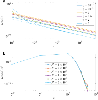
Figure 8: Deviation (99) from the asymptotic state of the mean-field dynamics of the BCS Hamiltonian with coupling $g(t)=\frac{\eta}{Nt}$ starting at $t=t_{0}=10^{-17}$ from the $t=0^{+}$ ground state. $N$ is the number of energy levels $\varepsilon_{k}=\frac{k}{N}$ and the number of fermions. Top panel: the deviation as a function of time for various values of $\eta$, $N=5\times 10^{4}$, and tolerance $2.22\times 10^{-14}$. The time dependence at $1\ll t\lesssim N$ fits a power law with exponent $-3.2$, which is somewhat overestimated due to faster decay at earlier times. At larger $t$ the deviation saturates. Bottom panel: deviation scaled by $N^{3}$ at $t=T=1.57N$ as a function of $\eta$ for various $N$. The dependence on $N$ is $\text{Dev}\propto N^{-3.0\pm 0.1}.$ We conclude from these data that the system can get arbitrarily close to the asymptotic state in a finite time in the $N\to\infty$ limit.

Analysis of results of simulations presented in Fig. 8 shows that at times $1\ll t\lesssim N$ the deviation decays as

$$\text{Dev}\approx\frac{R(\eta)}{t^{3.0}},$$ (100)

where $R(\eta)$ is a positive function of $\eta$ that is independent of $N$ for large $N$ as is evident from the lower panel of Fig. 8. At earlier times the decay of the deviation is even faster. For this reason, inclusion of earlier times in the analysis of $\text{Dev}(t)$ shown in the top panel of Fig. 8 produces higher powers of $t$, namely, $\text{Dev}\propto t^{-3.2}$. At $t\approx N$ the deviation saturates to a constant proportional to $N^{-3.0\pm 0.1}$. This result provides a more reliable way to determine the power law dependence of the deviation. Substituting $t=N$ into $\text{Dev}\propto t^{-y}$, we find $y=3.0$ as in Eq. (100).

Most importantly, we see that the system can get arbitrarily close to the late-time asymptotic state in finite time in the thermodynamic limit, i.e., the properties of $\Psi_{\infty}$ in this limit that we established above are accessible. Note that because the interaction vanishes at $t\to+\infty$, the system goes into an asymptotic state with $S_{k}^{z}=\text{const}$ for any $N$. Moreover, the thermodynamic and $t\to+\infty$ limits commute [84]. This implies independently of the numerical evidence that the system reaches an arbitrarily small vicinity of the asymptotic state in finite time. Separately, we observe that the deviation vanishes in the diabatic (noninteracting), $\eta\to 0$, and adiabatic, $\eta\to+\infty$ limits as expected.

We mentioned above that the deviation saturates at $t\propto N$ at which point $\text{Dev}\propto N^{-3.0}$. This along with Eq. (99) implies that corrections to our $N\to\infty$ analytic results in Sec. VI for $S_{k}^{z}$ and other spin components are of order $N^{-\frac{3}{2}}$. It is interesting to understand this scaling with $N$ as naively we would expect $N^{-1}$ scaling. These corrections to the $N\to\infty$ limit within mean field are not to be confused with the corrections to mean field due to quantum fluctuations. The latter corrections to $S_{k}^{z}$ are indeed of order $N^{-1}$, see Sec. VII.

XII Early-time quantum dynamics

Now let us investigate quantum effects at early times where the interaction part of the Hamiltonian dominates the dynamics being proportional to $\frac{1}{t}$ and the kinetic term $\hat{H}_{0}=\sum_{j}2\epsilon_{j}\hat{s}_{j}^{z}$ is negligible. Of special interest is the evolution starting from the BCS ground state at $t=0^{+}$ and observables that do not commute with the total fermion number operator, e.g., $\hat{s}_{k}^{-}$. We already saw in Sec. X, that such observables dephase with time. The magnitude of this quantum effect is controlled by a parameter distinct from the one that controls quantum fluctuations (corrections to mean field) in equilibrium. In this section, we illustrate this in a much simpler setting of the early-time dynamics. Then, we derive the von Neumann entanglement entropy $\mathtt{S}_{\mathrm{ent}}$ at early times and show that it monotonically increases with time and is $N$-independent in the thermodynamic limit. On the other hand, at finite but large $N$ we argue that $\mathtt{S}_{\mathrm{ent}}$ saturates at $\mathtt{S}_{\mathrm{ent}}=c(\eta)\ln N$, where $c(\eta)$ is a function of $\eta$ of order one. Dephasing and the growth of entanglement are two sides of the same coin. With time the phases of components of the many-body wave function with different particle numbers randomize, so that they no longer combine into a BCS product state and eventually saturate the entanglement entropy.

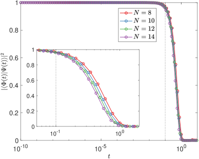
Figure 9: The absolute square of the overlap $\langle\Phi(t)|\Psi(t)\rangle$ between the early-time wave function $\Phi(t)$ [Eq. (103)] obtained by neglecting the non-interacting part of the BCS Hamiltonian and the result of the direct simulation of the nonstationary Schrödinger equation for the full BCS Hamiltonian with coupling $g(t)\propto\frac{\eta}{t}$, $N$ energy levels $\varepsilon_{k}=\frac{k}{N}$, and $\eta=1$. The initial condition is $\Phi(t_{0})=\Psi(t_{0})=\Psi_{\mathrm{BCS}}$, where $\Psi_{\mathrm{BCS}}$ is the infinite coupling mean-field ground state and $t_{0}=10^{-10}$. The doted vertical line marks $t=0.1$ below which the overlap is close to 1. This plot supports our estimate that the early-time approximation is valid for $t<t_{*}\approx\frac{0.1\eta}{W}$, where $W$ is the bandwidth of $\varepsilon_{k}$.

The Hamiltonian at early times approximately is

$$\hat{H}(t\to 0)\approx\hat{H}_{\mathrm{int}}=-\frac{\eta}{Nt}\hat{\jmath}_{+}\hat{\jmath}_{-},$$ (101)

where $\hat{\bm{\jmath}}=\sum_{k=1}^{N}\hat{\bm{s}}_{k}$ is the total spin, see the forth paragraph in Sec. IX for a brief discussion of the validity of this approximation. We rewrite the Schrödinger equation for $\hat{H}_{\mathrm{int}}$ as

$$i\frac{\partial\Psi}{\partial\tau}=-\frac{\hat{\jmath}_{+}\hat{\jmath}_{-}}{N}\Psi,\quad\tau=\eta\ln\frac{t}{t_{0}}.$$ (102)

Eigenvalues of $\hat{\jmath}_{+}\hat{\jmath}_{-}$ are $\jmath(\jmath+1)-\jmath_{z}^{2}+\jmath_{z}$. The ground state of $\hat{H}_{\mathrm{int}}$ with $\jmath_{z}=N_{\uparrow}-\frac{N}{2}$ and $\jmath=\frac{N}{2}$ is $\Psi_{0}(N_{\uparrow})$ in Eq. (28). The corresponding eigenvalue of $-\frac{\hat{\jmath}_{+}\hat{\jmath}_{-}}{N}$ is $E_{0}(N_{\uparrow})$ in Eq. (88). The infinite coupling BCS ground state (91) also has $\jmath=\frac{N}{2}$, but is not an eigenstate of $\hat{\jmath}_{z}$ (and fermion number operator). It follows from Eq. (92) that the solution of the nonstationary Schröndiner equation at early times that starts in the BCS ground state at $t=t_{0}$ is

$$\Phi(t)=2^{-\frac{N}{2}}\sum_{N_{\uparrow}=0}^{N}{\binom{N}{N_{\uparrow}}}^{\frac{1}{2}}e^{-iE_{0}(N_{\uparrow})\tau}\Psi_{0}(N_{\uparrow}).$$ (103)

We compare this early-time wave function, which we derived by neglecting the kinetic term $\hat{H}_{0}$, with the direct numerical solution of the nonstationary Schrödinger equation for the full quantum Hamiltonian $\hat{H}=\hat{H}_{0}+\hat{H}_{\mathrm{int}}$, same initial condition, for several $N$ in Fig. 9. Repeating the procedure that took us from Eq. (93) to Eq. (97), we obtain

$$\langle\hat{s}_{k}^{-}\rangle_{\Phi(t)}=\frac{1}{2}e^{-\frac{\tau^{2}}{2N}}$$ (104)

for the expectation value of the spin lowering operator $\hat{s}_{k}^{-}$ (equal time anomalous Green’s function) in the state $\Phi(t)$ in the thermodynamic limit.

The corresponding early-time classical motion is trivial. In the strong coupling limit $t\to 0^{+}$, we neglect $\varepsilon_{j}$ in Eq. (18). Spins in the classical ground state (31) with $J_{z}=0$ are along the $x$-axis, $\bm{S}_{j}=\langle\hat{\bm{s}}_{j}\rangle_{\mathrm{mf}}=\frac{\bm{x}}{2}$. Since the spins and the effective magnetic field $-2\bm{\Delta}$ are both parallel to the $x$-axis, the spins are stationary, i.e., $\langle\hat{s}_{k}^{-}\rangle_{\mathrm{mf}}=\frac{1}{2}$. We see that Eq. (104) is the early-time version of Eq. (97). At later times the Gaussian stops decaying as a function of $t$ and saturates at $t=t_{*}$. Therefore, the conclusion below Eq. (97) that the thermodynamic ($N\to\infty$) and $t_{0}\to 0^{+}$ limits do not commute applies here as well. In addition, we see that the $N\to\infty$ and $\eta\to+\infty$ (adiabatic) limits of the quantum solution do not commute as well, while taken in any order in the classical case they give $\langle\hat{s}_{k}^{-}\rangle_{\mathrm{mf}}=\frac{1}{2}$.

Let us also provide a simple estimate of the characteristic time $t_{*}$ until which the early-time approximation, i.e., the neglect of $\hat{H}_{0}$ compared to $\hat{H}_{\mathrm{int}}$ is reliable. The estimate is based on the mean-field (classical) equations of motion (18). We neglected $|\varepsilon_{j}|$ compared to $|\bm{\Delta}|$ in these equations. At short times the classical spins remain close to the $x$-axis and therefore $|\bm{\Delta}|\approx\frac{\eta}{2t}$. We require $|\varepsilon_{j}|\ll\frac{\eta}{2t_{*}}$. Replacing $|\varepsilon_{j}|$ with $\frac{W}{2}$, where $W$ is the bandwidth, we obtain $t_{*}\ll\frac{\eta}{W}$. Numerically, we find that

$$t_{*}\approx\frac{0.1\eta}{W}$$ (105)

is a reasonable estimate, see Figs. 9 and 10. Note that in these figures $\eta=1$ and $W=1-\frac{1}{N}$, so $t_{*}$ is about 10% larger than $t=0.1$, which is is hardly noticeable on the logarithmic scale.

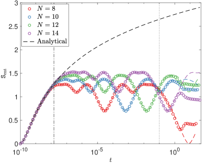
Figure 10: Entanglement entropy $\mathtt{S}_{\mathrm{ent}}$ at short times for the quantum BCS dynamics with time-dependent interaction strength $g(t)\propto\frac{\eta}{t}$. The initial state is the infinite coupling BCS ground state at $t=t_{0}$. System parameters are the same as in Fig. 9. Circles represent direct simulation of the dynamics with the full quantum BCS Hamiltonian, the corresponding colored dashed curves are $\mathtt{S}_{\mathrm{ent}}$ for the wave function (103) with a given $N$. Note that the early-time approximation (neglecting the kinetic term in the Hamiltonian) accurately captures all the structures in $\mathtt{S}_{\mathrm{ent}}$ to the left of dotted vertical line at $t=0.1$. Black dashed curve is the analytic answer (110) obtained by taking the $N\to\infty$ limit on top of the early-time approximation. It agrees with the numerically exact finite $N$ simulations until $\mathtt{S}_{\mathrm{ent}}$ stops growing at the Ehrenfest time $t_{E}$ [shown as a dash-dotted vertical line and given by Eq. (112) with $c_{E}=1.12$ and $N=10$] and finite size oscillations (partial recurrences) begin.

XII.1 Von Neumann entanglement entropy

We found in Sec. VII.2 that $\ln N$ scaling of the von Neumann entanglement entropy $\mathtt{S}_{\mathrm{ent}}$ for large $N$ is generic for the quantum BCS model. In particular, it holds for the late-time asymptotic state $\Psi_{\infty}$, projected BCS states, and exact infinite coupling ground state. We considered the case when the ratio of the number of fermion pairs $N_{\uparrow}$ (equivalently, the number of up pseudospins) to the number $N$ of single-particle energy levels $\frac{N_{\uparrow}}{N}=\frac{1}{2}$, but we expect the $\ln N$ scaling to be valid in the thermodynamic limit for other finite ratios as well. Next, we determine the early-time $\mathtt{S}_{\mathrm{ent}}$ for the quantum BCS time evolution with coupling $g(t)\propto\frac{\eta}{t}$ starting from the BCS ground state at $t=0^{+}$. We will find that $\mathtt{S}_{\mathrm{ent}}$ grows monotonically from zero with $\mathtt{S}_{\mathrm{ent}}\approx\ln\tau$ at large $\tau$. For finite $N$, the growth saturates at $\mathtt{S}_{\mathrm{ent}}\propto\ln N$ as before.

We postpone derivations to Appendix B and present only the main results and conclusions here. Let $N$ be even. Our first step is to calculate the reduced density matrix $\rho_{A}$ for the subsystem $A$ consisting of $\frac{N}{2}$ spins for the early-time many-body wave function (103),

$$\rho_{A}=2^{-\frac{N}{2}}\sum_{K,K^{\prime}=0}^{\frac{N}{2}}\Gamma_{K}\Gamma^{*}_{K^{\prime}}e^{-\frac{\tau^{2}}{4N}(K-K^{\prime})^{2}}\lvert K\rangle\langle K^{\prime}\rvert_{A},$$ (106)

where

$$\Gamma_{K}=\mbinom{\frac{N}{2}}{K}^{\frac{1}{2}}e^{-\frac{i\tau}{N}\left[K^{2}-K\left(\frac{3N}{2}+1\right)\right]}$$ (107)

and $|K\rangle_{A}$ is the state of the subsystem $A$ with a definite number $K$ of up spins that is symmetric with respect to arbitrary permutations of spins, i.e., with the maximum possible total spin $\frac{N}{4}$ and a definite value $K-\frac{N}{4}$ of its $z$-projection. Using this result, we evaluate $\mathrm{Tr}\left[\rho_{A}^{n}\right]$ in the limit $N\to\infty$ by replacing the sums with integrals and employing the multi-dimensional saddle point method,

$$\mathrm{Tr}\left[\rho_{A}^{n}\right]=\prod_{j=0}^{n-1}\left[1+\frac{\tau^{2}}{4}\sin^{2}\left(\frac{\pi j}{n}\right)\right]^{-\frac{1}{2}}.$$ (108)

Now consider the Rényi entanglement entropies for integer $n$ defined as

$$\mathtt{S}^{\mathrm{R}}_{n}=\frac{\ln\mathrm{Tr}\left[\rho_{A}^{n}\right]}{1-n}.$$ (109)

Treating $n$ as a replica index that can be analytically continued [85], we obtain the von Neumann entanglement entropy in the $n\to 1$ limit as

$$\begin{gathered}\mathtt{S}_{\mathrm{ent}}=\sqrt{1+\frac{\tau^{2}}{4}}\coth^{-1}\left[\sqrt{1+\frac{\tau^{2}}{4}}\right]+\ln\frac{\tau}{4}.\end{gathered}$$ (110)

We see that $\mathtt{S}_{\mathrm{ent}}$ is intensive in the thermodynamic limit. It monotonically grows from zero at $\tau=0$ $(t=t_{0})$ behaving as $\mathtt{S}_{\mathrm{ent}}\approx\ln\tau$ at large $\tau$.

There is a simple picture of the early-time dynamics that explains Eq. (110) and describes the saturation and subsequent oscillations of the entanglement entropy for finite $N$ seen in Fig. 10. First of all it is not difficult to see that $\mathtt{S}_{\mathrm{ent}}$ is bounded from above by $\ln\left(\frac{N}{2}+1\right)$. To show this, observe that the Hamiltonian with which the system evolves with respect to $\tau$ is $\hat{\jmath}_{+}\hat{\jmath}_{-}$ up to a multiplicative constant, see Eq. (102). The collective spin $\hat{\bm{\jmath}}=\hat{\bm{\jmath}}_{A}+\hat{\bm{\jmath}}_{\bar{A}}$, where $\hat{\bm{\jmath}}_{A}$ and $\hat{\bm{\jmath}}_{\bar{A}}$ are the total spins of subsystems $A$ and $\bar{A}$. Initially all spins-$\frac{1}{2}$ are along the $x$-axis and therefore the magnitudes of $\hat{\bm{\jmath}}$, $\hat{\bm{\jmath}}_{A}$, and $\hat{\bm{\jmath}}_{\bar{A}}$ are $\jmath=\frac{N}{2}$, $\jmath_{A}=\frac{N}{4}$, and $\jmath_{\bar{A}}=\frac{N}{4}$. These magnitudes are conserved. As a result the dynamics of subsystem $A$ is confined to a Hilbert space of dimension $\mathrm{dim}\mathcal{H}_{A}=2\jmath_{A}+1=\frac{N}{2}+1$. It is well-known [86] that the entanglement entropy is bounded from above by $\ln(\mathrm{dim}\mathcal{H}_{A})$, i.e., $\mathtt{S}_{\mathrm{ent}}\leq\ln\left(\frac{N}{2}+1\right)$.

We see that the $\ln N$ scaling of the entanglement entropy in the BCS theory (see also Sec. VII.2) is due to all to all interactions, which give rise to the collective spin $\hat{\bm{\jmath}}$. Note also that the BCS order parameter is related to the collective spin as $\Delta=g\langle\hat{\jmath}_{-}\rangle$. The $\ln N$ behavior of $\mathtt{S}_{\mathrm{ent}}$ is a general feature of late-time asymptotic states of the BCS dynamics as well as the ground state and other low energy stationary states unrelated to the nonautonomous character of the Hamiltonian we study in this paper. We nevertheless discuss it for completeness.

A useful general result [87] for the von Neumann entanglement entropy in collective spin models, such as the early-time Hamiltonian (101), is

$$\mathtt{S}_{\mathrm{ent}}=\sqrt{1+\langle\hat{n}_{\mathrm{ex}}\rangle}\coth^{-1}\!\left[\sqrt{1+\langle\hat{n}_{\mathrm{ex}}\rangle}\,\right]+\frac{1}{2}\ln\frac{\langle\hat{n}_{\mathrm{ex}}\rangle}{4},$$ (111)

where $\langle\hat{n}_{\mathrm{ex}}\rangle=\langle\hat{b}^{\dagger}\hat{b}\rangle$ is the number of excitations – the number of Holstein-Primakoff bosons for the collective spin $\hat{\bm{\jmath}}$ bosonized via a Holstein-Primakoff transformation around the direction of $\langle\hat{\bm{\jmath}}(\tau)\rangle$. To gain further insight into various features of $\mathtt{S}_{\mathrm{ent}}$, consider the semiclassical motion of this bosonic mode. This motion is one-dimensional and Hamiltonian. Nearby trajectories separate linearly in time, i.e., the growth of the momentum and position with $\tau$ is linear. Since $\langle\hat{n}_{\mathrm{ex}}\rangle$ is quadratic in the momentum and position, we expect $\langle\hat{n}_{\mathrm{ex}}\rangle\sim\tau^{2}$. Indeed, comparing Eqs. (111) and (110), we see that $\langle\hat{n}_{\mathrm{ex}}\rangle=\frac{\tau^{2}}{4}$.

Bounded one-dimensional Hamiltonian motion is periodic, which explains the post-saturation oscillations of $\mathtt{S}_{\mathrm{ent}}$ (see Fig. 10) approximately with the period of the underlying classical trajectory [87]. The time at which quantum fluctuations of the collective spin $\hat{\bm{\jmath}}$ become comparable to its magnitude, i.e., $\langle\hat{n}_{\mathrm{ex}}\rangle\sim\frac{N}{2}$, is the Ehrenfest time $\tau_{E}$. Using $\langle\hat{n}_{\mathrm{ex}}\rangle=\frac{\tau^{2}}{4}$ and $\tau=\eta\ln\frac{t}{t_{0}}$, we obtain

$$\tau_{E}=c_{E}\sqrt{2N},\quad t_{E}=t_{0}e^{c_{E}\frac{\sqrt{2N}}{\eta}},$$ (112)

where $c_{E}$ is a coefficient of order one. Recall that the entanglement entropy in the thermodynamic limit (110) grows as $\ln\tau$ for large $\tau$. This growth stops and finite size effects kick in at the Ehrenfest time scale as at this point the number of bosonic excitations reaches its maximum possible value. Note also that $t_{E}$ is the time when the argument of the exponential function in Eq. (104) becomes of order one, i.e., the quantum dephasing effect becomes appreciable. Numerically, we observe that Eq. (112) provides a reasonable estimate of the time when the finite $N$ entanglement entropy deviates from the $N\to\infty$ result (110), see, e.g., the $t=t_{E}$ line for $N=10$ and $c_{E}=1.12$ in Fig. 10 (dash-dotted vertical line). We can also estimate the saturation value of the von Neumann entanglement entropy for large $N$ as $\mathtt{S}_{\mathrm{ent}}\sim\ln\tau_{E}\sim\frac{1}{2}\ln N$, cf. Eqs. (72) and (76).

XIII Conclusion

In this paper, we demonstrated that the far from equilibrium dynamics of BCS superconductors is classical in the thermodynamic limit under certain conditions. Specifically, we obtained exact solutions for the quantum and classical (mean-field) dynamics of the BCS Hamiltonian with time-dependent coupling, $g(t)=\frac{1}{\nu t}$ launched from the ground state at $t=t_{0}\to 0^{+}$. We explicitly determined exact quantum and mean-field wave functions at long times, evaluated quantum averages of a generic local observable in them, and proved that they coincide in the thermodynamic limit. It is clear that this must remain true for a broad class of $g(t)$ and initial conditions. Nevertheless, it is worthwhile to verify that the mean field is similarly exact when $g(t)$ does not vanish at $t\to+\infty$. This can be done, for example, by solving for the backward time evolution from $t=+\infty$ to $t=0^{+}$ of our model using the method we developed in this paper.

On the other hand, the classical picture breaks down dramatically for global quantities, such as the bipartite von Neumann entanglement entropy as we saw above and the Loschmidt echo as shown in Ref. 39. Also noteworthy is the behavior of anomalous averages – expectation values of operators that do not conserve the total fermion number, such as the equal time anomalous Green’s function. For these kinds of observables, the thermodynamic limit does not commute with the adiabatic ($\nu\to 0^{+}$) and $t_{0}\to 0^{+}$ limits due to quantum dephasing. Their quantum fluctuations are controlled by a new parameter that can be much larger than the inverse particle number – the parameter controlling the magnitude of equilibrium quantum fluctuations (finite size corrections).

These results provide a deeper understanding of the reasons behind the success of mean-field theories in general, beyond our focus on far from equilibrium superconductivity. In situations where they are believed to be accurate (e.g., above a certain dimension), we expect the mean-field wave function to capture the order parameter and other local observables, but not the entanglement and other global properties of the true many-particle state. A fascinating project is to investigate the interplay between quantumness and nonlocality in other “mean-field” models, such as topological $p$-wave superconductors [7, 61], infinite-dimensional Hubbard model [88], and magnon Bose-Einstein condensates [89, 90]. In particular, an interesting question to ask in this connection is how well the mean-field approximation describes non-trivial topological properties, which are inherently non-local.

We saw that the unitary time evolution brings our system into a steady state similar to one of the nonequilibrium phases in interaction quenched BCS superfluids [35]. This state is a gapless superconductor with vanishing superfluid density, order parameter, and pair-breaking excitation gap. As a consequence, its superfluid properties can only be revealed in energy resolved observables, such as the spectral supercurrent density. The steady state is nonthermal but is described by a nontrivial emergent generalized Gibbs ensemble, where the emergent integrals of motion are the single-particle level occupancy operators. We only touched on the prospects of realizing our model and testing our predictions in experiment in Introduction and Sec. III, so this remains an important topic for future research.

We determined the dynamics of the von Neumann entanglement entropy $\mathtt{S}_{\mathrm{ent}}$ starting from the unentangled BCS (mean-field) ground state. Interestingly, the growth of the entanglement is entirely due to the interaction part of the quantum BCS Hamiltonian. The entanglement entropy is finite in the thermodynamic limit and grows monotonically as a function of time. Note that within the mean-field treatment $\mathtt{S}_{\mathrm{ent}}=0$ at all times. In a finite system, $\mathtt{S}_{\mathrm{ent}}$ saturates at a value that scales as $\ln V$ with the system volume $V$.

This paper paves the way to a comprehensive theory of integrability of nonautonomous quantum Hamiltonians. We demonstrated that the off-shell Bethe Ansatz [53, 52, 55, 56], which provides an integral representation of solutions of the nonstationary Schrödinger equation, is a key ingredient of this theory. Another key ingredient is the systematic method we developed here to obtain explicit physical results, such as the ones listed above in this section, from the integral representation. Our method should work equally well for other models that go through the off-shell Bethe Ansatz, e.g., the problem of molecular production in an atomic Fermi gas swept through a Feshbach resonance and Demkov-Osherov, bow-tie, and generalized bow-tie multi-level Landau-Zener models [52]. It is interesting to apply our approach to these models and even more important to generalize and broaden the scope of the off-shell Bethe Ansatz to include time-dependent models unrelated to the Gaudin algebra.

Appendix A Solution of the classical equations of motion

As discussed in the main text, there are two ways to make Anderson pseudospins classical. One option is to replace spin-$\frac{1}{2}$ with spin-$s$ and take the limit $s\to\infty$. The other option is to perform mean-field decoupling, $\langle\hat{A}_{1}\hat{A}_{2}\rangle\to\langle\hat{A}_{1}\rangle\langle\hat{A}_{2}\rangle$, in the Heisenberg equations of motion for Anderson pseudospins. Both approaches result in the same equations of motion (18). Here we solve these classical equations of motion exactly and determine classical spins $\bm{S}_{j}$ explicitly at long times. In the main text, we compare this answer with the thermodynamic limit of the exact quantum (spin-$\frac{1}{2}$) solution. We note that our result in this appendix also solves the generalized SU(2) Knizhnik-Zamolodchikov equations in the limit of classical spins and the boundary field $B\equiv\nu t\to+\infty$ [52, 55, 56]. Because we expect classical (mean-field) dynamics to be able to reproduce quantum dynamics only for $N\to\infty$, we primarily focus on this limit, even though our method is suitable for finite $N$ as well.

Equation (33) is an exact integral representation for the solution of the nonstationary Schrödinger equation for spins of arbitrary magnitudes. Let magnitudes of all spins be $s$. Our aim is to take the classical limit $s\to\infty$ and $\hbar\to 0$ of the solution keeping $\hbar s=S$ fixed. The first step is to restore $\hbar$ in the Schrödinger equation,

$$i\hbar\frac{d\Psi}{dt}=\Biggl{[}\sum_{j=1}^{N}2\varepsilon_{j}(\hbar\hat{s}_{j}^{z})-\frac{1}{\nu t}\sum_{j,k=1}^{N}(\hbar\hat{s}_{j}^{+})(\hbar\hat{s}_{k}^{-})\Biggr{]}\Psi.$$ (113)

Note that $\hbar$ is dimensionless in our units. Canceling one factor of $\hbar$ on both sides and comparing to Eq. (13) with $g(t)=\frac{1}{\nu t}$, we see that the restoration of $\hbar$ amounts to the replacement $\nu\to\frac{\nu}{\hbar}$. Making this replacement in Eq. (33), we further observe that the Yang-Yang action becomes,

$${\cal S}(\bm{\lambda},\bm{\varepsilon},t)=2\nu t\sum_{\alpha}\lambda_{\alpha}+2S\sum_{j}\sum_{\alpha}\ln(\varepsilon_{j}-\lambda_{\alpha})-\hbar\sum_{\alpha}\sum_{\beta\neq\alpha}\ln(\lambda_{\beta}-\lambda_{\alpha}),$$ (114)

where

$$S=\hbar s.$$ (115)

Expressions for $\Psi(t)$, $\Xi(\bm{\lambda},\varepsilon)$, and $\hat{L}^{+}(\lambda)$ stay the same.

Similar to the spin-$\frac{1}{2}$ case in Sec. V, the integral in Eq. (33) localizes to the vicinities of the stationary points. The stationary point equations $\frac{\partial\mathcal{S}}{\partial{\lambda_{\alpha}}}=0$ now are

$$\nu t+S\sum_{j}\frac{1}{\lambda_{\alpha}-\varepsilon_{j}}=\hbar\sum_{\beta\neq\alpha}\frac{1}{\lambda_{\alpha}-\lambda_{\beta}},\quad\alpha=1,\dots,N_{\uparrow}.$$ (116)

The difference with Eq. (36) is in the number $N_{\uparrow}$ of rapidities $\lambda_{\alpha}$. In Eq. (36), $N_{\uparrow}$ is the number of up spins which is smaller than the number $N$ of $\varepsilon_{j}$. In Eq. (116), $N_{\uparrow}$ is the amount by which the $z$-component $\jmath_{z}$ of the total spin is raised, $\jmath_{z}=N_{\uparrow}-Ns$. Since the magnitude $s$ of spins diverges, $N_{\uparrow}$ also diverges and there are many more $\lambda_{\alpha}$ than $\varepsilon_{j}$.

As before, each $\lambda_{\alpha}$ must tend to one of $\varepsilon_{j}$ as $t\to+\infty$. Suppose $n_{j}$ of $\lambda_{\alpha}$ tend to $\varepsilon_{j}$. We denote the elements of this $j^{\mathrm{th}}$ degenerate subset of $\lambda_{\alpha}$ as $\lambda_{k}^{j}$, where $k=1,\dots,n_{j}$. Note that $\sum_{j=1}^{N}n_{j}=N_{\uparrow}$. Let

$$\lambda_{k}^{j}=\varepsilon_{j}+\chi_{k}^{j},\quad\chi_{k}^{j}=\frac{\hbar z_{k}^{j}}{2\nu t}.$$ (117)

We will see shortly that the new variables $z_{k}^{j}$ are independent of $t$ to the leading order in $t^{-1}$. All terms in Eq. (116) that contain $\lambda_{\alpha}-\varepsilon_{j}$ with $\lambda_{\alpha}$ not in the degenerate subset corresponding to $\varepsilon_{j}$ or terms that contain $\lambda_{\alpha}-\lambda_{\beta}$ with $\lambda_{\alpha}$ and $\lambda_{\beta}$ not in the same degenerate subset are negligible. Therefore, to the leading order in $t^{-1}$, Eq. (116) splits into $N$ decoupled sets of equations for $z_{k}^{j}$,

$$1+\frac{2s}{z_{k}^{j}}=\sum_{k^{\prime}\neq k}\frac{2}{z_{k}^{j}-z_{k^{\prime}}^{j}},\quad k=1,\dots,n_{j}.$$ (118)

This is a set of $n_{j}$ equations for $n_{j}$ variables for each $j=1,\dots,N$. It is clear from Eq. (118) that $z_{k}^{j}$ are $t$-independent. In fact, $z_{k}^{j}$ are the roots of the associated Laguerre polynomial $L^{-2s-1}_{n_{j}}(z)$ [70]. We will not need this property below as we will not evaluate integrals over $\chi_{k}^{j}$ by the steepest descent method.

Let us see how the vector $\Xi(\bm{\lambda},\bm{\varepsilon})$ given by Eq. (34) behaves near stationary points. Observe that $\hat{L}^{+}(\lambda_{\alpha})\to\frac{\hat{s}_{j}^{+}}{\chi_{k}^{r}}$ when $\lambda_{\alpha}\to\varepsilon_{r}$. Therefore,

$$\Xi(\bm{\lambda},\bm{\varepsilon})\to\sum_{\{n_{j}\}}\left[\frac{N_{\uparrow}!}{\prod_{j}n_{j}!}\prod_{j}\frac{(\hat{s}_{j}^{+})^{n_{j}}}{\prod_{k}\chi_{k}^{j}}\right]|0\rangle.$$ (119)

The summation here is over all sets $\{n_{j}\}$ of $N$ positive integers such that

$$\sum_{j=1}^{N}n_{j}=N_{\uparrow}.$$ (120)

This corresponds to summing over all stationary points. The combinatorial factor in Eq. (119) is the number of ways to choose $N$ groups of variables out of $N_{\uparrow}$ variables with $n_{j}$ elements in the $j^{\mathrm{th}}$ group. The action of powers of spin-$s$ raising operators $s_{r}^{+}$ on the state $|0\rangle$ where all spins point in the negative $z$-direction is

$$\prod_{r=1}^{N}(\hat{s}_{r}^{+})^{n_{r}}|0\rangle=|n_{1}\dots n_{N}\rangle\prod_{r=1}^{N}\sqrt{\frac{(2s)!n_{r}!}{(2s-n_{r})!}},$$ (121)

where $|n_{1}\dots n_{N}\rangle$ is a normalized eigenstate of all $\hat{s}_{r}^{z}$ with eigenvalues $m_{r}=n_{r}-s$. Eq. (119) becomes

$$\Xi(\bm{\lambda},\bm{\varepsilon})\to\sum_{\{n_{j}\}}\prod_{j=1}^{N}\sqrt{\frac{(2s)!}{(2s-n_{j})!n_{j}!}}\,\,\frac{|n_{1}\dots n_{N}\rangle}{\prod_{k}\chi_{k}^{j}}.$$ (122)

We manipulate the Yang-Yang action (114) similarly to how we manipulated the stationary point equations (116) neglecting $\chi_{k}^{l}$ in $\varepsilon_{j}-\lambda_{\alpha}$ when $\lambda_{\alpha}$ does not belong to the $j^{\mathrm{th}}$ degenerate subset and in $\lambda_{\alpha}-\lambda_{\beta}$ when $\lambda_{\alpha}$ and $\lambda_{\beta}$ are not in the same degenerate subset. We find

$${\cal S}(\bm{\chi},\bm{\varepsilon},t)=2\nu t\sum_{j}n_{j}\varepsilon_{j}+2S\sum_{j}\sum_{k\neq j}n_{k}\ln(\varepsilon_{j}-\varepsilon_{k})-\hbar\sum_{j}\sum_{k\neq j}n_{j}n_{k}\ln(\varepsilon_{j}-\varepsilon_{k})+\sum_{j}\mathcal{S}^{j}_{\mathrm{deg}},$$ (123)

where

$$\mathcal{S}^{j}_{\mathrm{deg}}=\hbar\sum_{k}z_{k}^{j}+2S\sum_{k}\ln(-\chi_{k}^{j})-\hbar\sum_{k}\sum_{k^{\prime}\neq k}\ln(\chi_{k}^{j}-\chi_{k^{\prime}}^{j}).$$ (124)

Recall that $\nu$ is of order $N$ and therefore the first three terms in ${\cal S}(\bm{\chi},\bm{\varepsilon},t)$ are of order $N^{2}$ because each summation over the single-particle level index gives a factor of $N$. On the other hand, sums over the degenerate subspace in $\mathcal{S}^{j}_{\mathrm{deg}}$ are of order $s$ and consequently $\sum_{j}\mathcal{S}^{j}_{\mathrm{deg}}$ is of order $Ns$. Take the limits $N\to\infty$ and $s\to\infty$ so that $\frac{s}{N}\to 0$. The last term in Eq. (123) is then negligible when $N\to\infty$. As for the case of spin-$\frac{1}{2}$ in Sec. V, we need to choose the branch of the logarithm so that $\ln(-1)=-i\pi$. It is not difficult to show that to order $N^{2}$ the imaginary part of the third term on the right hand side of Eq. (123) contributes only to the overall normalization constant. Together these observations allow us to rewrite Eq. (123) as

$$\hbar{\cal S}(\bm{\chi},\bm{\varepsilon},t)=2\nu t\sum_{j}S_{j}^{z}\varepsilon_{j}-2\sum_{k>j}S_{j}^{z}S_{k}^{z}\ln|\varepsilon_{j}-\varepsilon_{k}|-2i\pi S\sum_{j}jS_{j}^{z},$$ (125)

where $S_{j}^{z}=\hbar m_{j}$ are the $z$-components of the classical spins in the limit $\hbar\to 0$.

We also need to express the square root of the binomial coefficient in Eq. (122) in terms of $S_{j}^{z}=\hbar m_{j}=\hbar n_{j}-S$. Using Stirling’s approximation, we obtain

$$\sqrt{\frac{(2s)!}{(2s-n_{j})!n_{j}!}}=\exp\left[-\frac{(S+S_{j}^{z})\ln(S+S_{j}^{z})+(S-S_{j}^{z})\ln(S-S_{j}^{z})}{2\hbar}\right].$$ (126)

Let us summarize what we did so far. We evaluated the ingredients in the general expression (33) for $\Psi(t)$ in the vicinity of the stationary points of the Yang-Yang action $\mathcal{S}(\bm{\lambda},\bm{\varepsilon},t)$ since at large $t$ the integral localizes to these vicinities. In Eq. (126), we took advantage of the fact that in the classical limit $\hbar\to 0$ the magnitude of the quantum spin $\hat{\bm{s}}^{z}_{j}$ diverges, $s\to\infty$, while the magnitude $S=\hbar s$ and components, e.g., $S_{j}^{z}=\hbar m_{j}$, of the classical spin $\bm{S}_{j}$ remain finite. Substituting Eqs. (122) and (125) into Eq. (33) and using Eq. (126), we find

$$\Psi(t)=\sum_{\{m_{j}\}}e^{-\frac{iEt}{\hbar}}e^{\frac{i\Omega}{\hbar\nu}}e^{-\frac{A}{2\hbar}}|m_{1}\dots m_{N}\rangle,$$ (127)

where the sum is over all $z$-projections $m_{j}$ such that $\sum_{j}m_{j}=\jmath_{z}$ and we integrated over all $\chi_{k}^{j}$ to derive Eq. (127) . Since we neglected $\mathcal{S}^{j}_{\mathrm{deg}}$, these integrals are $\oint\frac{d\chi_{k}^{j}}{\chi_{k}^{j}}=2\pi i$ and contribute only to the overall multiplicative constant. The contours of integration over $\chi_{k}^{j}$ are guaranteed to enclose the origin as we start the time evolution in the instantaneous ground state at $t=0^{+}$, see the discussion below Eq. (36). Quantities $A$, $E$, and $\Omega$ are

$$E =\sum_{j}2\varepsilon_{j}S_{j}^{z},$$ (128a)

$$\Omega =2\sum_{k>j}S_{j}^{z}S_{k}^{z}\ln|\varepsilon_{j}-\varepsilon_{k}|,$$ (128b)

$$A =(S+S_{j}^{z})\ln(S+S_{j}^{z})+(S-S_{j}^{z})\ln(S-S_{j}^{z})+\frac{4\pi jSS_{j}^{z}}{\nu}.$$ (128c)

In the limit $\hbar\to 0$ only terms that minimize $A$ survive in Eq. (127). Minimizing Eq. (128c) with respect to $S_{j}^{z}$ at fixed $\sum_{j}S_{j}^{z}$, we obtain

$$S_{j}^{z}=-S\tanh(2Sa_{j}),\quad a_{j}\equiv\frac{\pi(j-\mu)}{\nu},$$ (129)

where $\mu$ is the Lagrange multiplier (chemical potential) corresponding to $\sum_{j}S_{j}^{z}$ and we used $\tanh^{-1}z=\frac{1}{2}\ln\left(\frac{1+z}{1-z}\right)$.

The state of the system (127) is now a sum over only $m_{j}$ such that $\hbar m_{j}\to S_{j}^{z}$ with $S_{j}^{z}$ given by Eq. (129). Note that this is more than one value of $m_{j}$, because, for example, $m_{j}$ and $m_{j}+1$ correspond to the same $S_{j}^{z}$ in the limit $\hbar\to 0$. This allows us to also evaluate the $x$ and $y$ components of classical spins by taking the expectation value $\langle\hat{s}_{j}^{-}\rangle$ of the quantum spin in this state. We have

$$S_{j}^{x}-iS_{j}^{y}\equiv S_{j}^{-}=|S_{j}^{-}|e^{-\frac{i\Delta Et}{\hbar}}e^{\frac{i\Delta\Omega}{\hbar\nu}},$$ (130)

where $\Delta E=E(m_{j}+1)-E(m_{j})$ and $\Delta\Omega=\Omega(m_{j}+1)-\Omega(m_{j})$ are the amounts by which $E$ and $\Omega$ change when we increase $m_{j}$ by 1 or, equivalently, increase $S_{j}^{z}$ by $\hbar$. We have

$$S_{j}^{-}=\frac{Se^{-2i\varepsilon_{j}t+i\varphi_{j}}}{\cosh(2S\zeta_{j})},\quad\varphi_{j}=\frac{2\eta}{N}\sum_{k\neq j}S_{k}^{z}\ln|\varepsilon_{k}-\varepsilon_{j}|,\quad S_{j}^{z}=-S\tanh(2S\zeta_{j}),\quad\zeta_{j}\equiv\frac{\pi\eta(j-\mu)}{N}.$$ (131)

Here we traded $\nu$ for $\frac{N}{\eta}$. This is the exact solutions of the Hamilton’s equations of motion (18) for the classical time-dependent BCS Hamiltonian (15) for $t\to+\infty$ and $N\to\infty$ (these two limits commute as we discuss in Sec. IX for the quantum and at the end of Sec. XI for the classical dynamics). As noted below Eq. (21), to compare to mean-field dynamics starting from the BCS product state, we need to set the spin length $S=\frac{1}{2}$ in Eq. (131).

Appendix B Rényi entanglement entropy

One of the key differences between quantum and classical systems is the presence of entanglement in the quantum case, i.e., of statistical correlations between subsystems that prevent the system from being in a state that is a product of the states of the individual subsystems. The degree of quantum entanglement between two subsystems $(A,\bar{A})$ is quantified by the von Neumann entanglement entropy defined as $\mathtt{S}_{\mathrm{ent}}=\mathrm{Tr}\rho_{A}\ln\rho_{A}$ where $\rho_{A}=\mathrm{Tr}_{\bar{A}}\rho$ is the reduced density matrix of $A$ and $\rho$ is the density matrix of the combined system. Rather than computing $\mathtt{S}_{\mathrm{ent}}$ directly, it is more convenient to work with the Rényi entanglement entropy $\mathtt{S}^{\mathrm{R}}_{n}$ defined in Eq. (109). Its usefulness lies in the index $n$ which can be treated as a replica index to evaluate the von Neumann entropy in the limit $n\to 1$. The Rényi entropy also encodes other entanglement measures such as the Hartley entropy for $n=0$ and the purity for $n=2$. In what follows, we derive an expression for the Rényi entanglement entropy for arbitrary $n$ (and the von Neumann entanglement entropy by analytic continuation) for a bipartition of the early-time wave function (103) for the dynamics with the quantum BCS Hamiltonian (11) [or equivalently with Hamiltonian (13) for $s=\frac{1}{2}$] with $g(t)=\frac{\eta}{Nt}$ starting from the infinite coupling BCS ground state (91) at $t=t_{0}\to 0^{+}$.

B.1 Reduced density matrix

In order to determine the Rényi entropy $\mathtt{S}^{\mathrm{R}}_{n}$, we require the reduced density matrix $\rho_{A}$ for a bipartition of the system. As in Sec. VII.2, we choose $A$ to be the set of spins $\hat{\bm{s}}_{j}$ that correspond the lower half of the single-particle energy spectrum $\varepsilon_{j}$. We need to evaluate $\rho_{A}$ for the state (103). To do so, we first rewrite Eq. (103) in a more convenient form by substituting Eq. (74) into it and rearranging the coefficients by first splitting the sum into two terms ($N_{\uparrow}\leq\frac{N}{2}$ and $N_{\uparrow}>\frac{N}{2}$) and then recombining it,

$$\Phi(t)=2^{-\frac{N}{2}}\sum_{N_{\uparrow}^{A}=0}^{\frac{N}{2}}\binom{\frac{N}{2}}{N_{\uparrow}^{A}}^{\frac{1}{2}}\left|N_{\uparrow}^{A}\right\rangle_{A}\otimes\sum_{N_{\uparrow}^{\bar{A}}=0}^{\frac{N}{2}}e^{-iE_{0}(N_{\uparrow})\tau}\binom{\frac{N}{2}}{N_{\uparrow}^{\bar{A}}}^{\frac{1}{2}}\left|N_{\uparrow}^{\bar{A}}\right\rangle_{\bar{A}},$$ (132)

where $N_{\uparrow}=N_{\uparrow}^{A}+N_{\uparrow}^{\bar{A}}$ and $\tau=\eta\ln\frac{t}{t_{0}}$. At $\tau=0$ the system is in the product state (91) [all spins point along $x$] and we see that the two sums decouple in this case as they should. The density matrix of the system is then

$$\rho(t)=2^{-N}\sum_{K,K^{\prime}=0}^{\frac{N}{2}}\binom{\frac{N}{2}}{K}^{\frac{1}{2}}\binom{\frac{N}{2}}{K^{\prime}}^{\frac{1}{2}}\lvert K\rangle\langle K^{\prime}\rvert_{A}\otimes\sum_{Q,Q^{\prime}=0}^{\frac{N}{2}}e^{-i\left[E_{0}(K+Q)-E_{0}(K^{\prime}+Q^{\prime})\right]\tau}\binom{\frac{N}{2}}{Q}^{\frac{1}{2}}\binom{\frac{N}{2}}{Q^{\prime}}^{\frac{1}{2}}\lvert Q\rangle\langle Q^{\prime}\rvert_{\bar{A}},$$ (133)

where we renamed the summation indices $N_{\uparrow}^{A}\to K$ and $N_{\uparrow}^{\bar{A}}\to Q$ for simplicity. It remains to trace over $\bar{A}$ to find the reduced density matrix of $A$. Performing the trace yields a factor of $\delta_{Q,Q^{\prime}}$ which consumes the sum over $Q^{\prime}$. In the large $N$ limit, we replace the remaining sum over $Q$ with an integral over $z=\frac{2Q}{N}$ and evaluate it using the saddle point method to arrive at

$$\rho_{A}(t)=2^{-\frac{N}{2}}\sum_{K,K^{\prime}=0}^{\frac{N}{2}}\sqrt{\binom{\frac{N}{2}}{K}}e^{-\frac{i\tau}{N}\left[K^{2}-K(\frac{3N}{2}+1)\right]}\sqrt{\binom{\frac{N}{2}}{K^{\prime}}}e^{\frac{i\tau}{N}\left[K^{\prime 2}-K^{\prime}(\frac{3N}{2}+1)\right]}e^{-\frac{\tau^{2}}{4N}(K-K^{\prime})^{2}}\lvert K\rangle\langle K^{\prime}\rvert_{A}.$$ (134)

B.2 Rényi entropy

Having determined $\rho_{A}(t)$, we now turn to calculating the Rényi entanglement entropy defined by Eq. (109). When taking the trace of powers of $\rho_{A}$ the phases cancel so that

$$\mathrm{Tr}\left[\rho_{A}^{n}\right]=2^{-n\frac{N}{2}}\sum_{x_{1},\ldots,x_{n}}^{\frac{N}{2}}\binom{\frac{N}{2}}{x_{1}}\ldots\binom{\frac{N}{2}}{x_{n}}\exp\left[-\frac{\tau^{2}}{4N}\left[(x_{1}-x_{2})^{2}+\ldots+(x_{n}-x_{1})^{2}\right]\right].$$ (135)

As before, in the large $N$ limit we replace the sums with integrals and evaluate them using the multi-dimensional saddle point method. The stationary point occurs at $x_{1}=x_{2}=\ldots=x_{n}=\frac{1}{2}$ and the matrix elements of the Hessian matrix are

$$\mathrm{Hess}_{ij}=-\left(4+\frac{\tau^{2}}{2}\right)\delta_{i,j}+\frac{\tau^{2}}{4}\delta_{i+1,j}+\frac{\tau^{2}}{4}\delta_{i-1,j}$$ (136)

with eigenvalues given by [91]

$$\kappa_{j}=-\left(4+\frac{\tau^{2}}{2}\right)+\frac{\tau^{2}}{4}\omega^{j}+\frac{\tau^{2}}{4}\omega^{(n-1)j}$$ (137)

where $\omega=e^{\frac{2\pi i}{n}}$ is a primitive $n^{\text{th}}$ root of unity. Substituting $\prod_{j}\kappa_{j}$ for the determinant into the saddle point formula and simplifying we have

$$\mathrm{Tr}\left[\rho_{A}^{n}\right]=\prod_{j=0}^{n-1}\left[1+\frac{\tau^{2}}{16}\left(2-e^{i\frac{2\pi j}{n}}-e^{-i\frac{2\pi j}{n}}\right)\right]^{-\frac{1}{2}}$$ (138)

from which the Rényi entanglement entropy follows

$$\mathtt{S}^{\mathrm{R}}_{n}(\tau)=\frac{-1}{2(1-n)}\sum_{j=0}^{n-1}\ln\left[1+\frac{\tau^{2}}{16}\left(2-e^{i\frac{2\pi j}{n}}-e^{-i\frac{2\pi j}{n}}\right)\right].$$ (139)

To evaluate the von Neumann entanglement entropy we analytically continue to $n=1$ by writing the sum as a contour integral [85]

$$\mathtt{S}^{\mathrm{R}}_{n}(\tau)=\frac{-1}{2(1-n)}\sum_{j=0}^{n-1}\oint\frac{\mathrm{d}u}{2\pi i}\frac{\ln\left[1+\frac{\tau^{2}}{16}\left(2-u-u^{-1}\right)\right]}{u-e^{i2\pi j/n}}=\frac{-1}{2(1-n)}\oint\frac{\mathrm{d}u}{2\pi i}\left(\frac{nu^{n-1}}{u^{n}-1}\right)\ln\left[1+\frac{\tau^{2}}{16}\left(2-u-u^{-1}\right)\right].$$ (140)

In the limit $n\to 1$ [85]

$$\mathtt{S}^{\mathrm{R}}_{n\to 1}(\tau)\to-\frac{1}{2}\oint\frac{\mathrm{d}u}{2\pi i}\left(\frac{n}{n-1}\frac{1}{1-u}+\frac{\ln u}{(u-1)^{2}}+\mathcal{O}(n-1)\right)\ln\left[1+\frac{\tau^{2}}{16}\left(2-u-u^{-1}\right)\right],$$ (141)

which becomes

$$\mathtt{S}^{\mathrm{R}}_{n\to 1}(\tau)=\mathtt{S}_{\mathrm{ent}}(\tau)=\int_{1}^{\infty}\mathrm{d}\lambda\frac{\ln\left[1+\frac{\tau^{2}}{16}\left(2+\lambda+\lambda^{-1}\right)\right]}{(\lambda+1)^{2}}=\sqrt{1+\frac{\tau^{2}}{4}}\coth^{-1}\sqrt{1+\frac{\tau^{2}}{4}}+\ln\frac{\tau}{4}.$$ (142)

An immediate observation is that $\mathtt{S}_{\mathrm{ent}}(\tau)$ is finite in the thermodynamic limit. In the main text we provide a thorough qualitative explanation of Eq. (142) and use it together with other considerations to understand the behavior of $\mathtt{S}_{\mathrm{ent}}(\tau)$ for finite $N$ as well, namely, its saturation at $\mathtt{S}_{\mathrm{ent}}\sim\frac{1}{2}\ln N$ at $\tau\sim\sqrt{N}$ and subsequent oscillations as a function of $\tau$.

References

- [1] J. Bardeen, L. N. Cooper, and J. R. Schrieffer, Theory of Superconductivity, Phys. Rev. 108, 1175 (1957).
- [2] P. W. Anderson, Random-Phase Approximation in the Theory of Superconductivity, Phys. Rev. 112, 1900 (1958).
- [3] E. A. Yuzbashyan, B. L. Altshuler, V. B. Kuznetsov, and V. Z. Enolskii, Nonequilibrium Cooper pairing in the nonadiabatic regime, Phys. Rev. B 72, 220503(R) (2005).
- [4] P. Coleman, Introduction to Many-Body Physics (Cambridge University Press, 1st ed., 2016).
- [5] The mean-field ground state and excited states of the condensate correspond to equilibria of the classical spins. Removing or adding a fermion corresponds to removing a classical spin.
- [6] A. L. DiRienzo and R. A. Young, A coupled angular momentum model for the Josephson junction, Am. J. Phys. 51, 587 (1983).
- [7] N. Read and D. Green, Paired states of fermions in two dimensions with breaking of parity and time-reversal symmetries and the fractional quantum Hall effect, Phys. Rev. B 61, 10267 (2000).
- [8] R. W. Richardson, Pairing in the limit of a large number of particles, J. Math. Phys. 18, 1802 (1977).
- [9] J. Roman, G. Sierra, and J. Dukelsky, Large N limit of the exactly solvable BCS model: Analytics versus numerics, Nucl. Phys. B 634, 483 (2002).
- [10] E. A. Yuzbashyan, A. A. Baytin, and B. L. Altshuler, Finite-size corrections for the pairing Hamiltonian, Phys. Rev. B 71, 094505 (2005).
- [11] R. A. Barankov, L. S. Levitov, and B. Z. Spivak, Collective Rabi Oscillations and Solitons in a Time-Dependent BCS Pairing Problem, Phys. Rev. Lett. 93, 160401 (2004).
- [12] A. V. Andreev, V. Gurarie, and L. Radzihovsky, Nonequilibrium Dynamics and Thermodynamics of a Degenerate Fermi Gas Across a Feshbach Resonance, Phys. Rev. Lett. , 130402 (2004).
- [13] M. H. Szymanska, B. D. Simons, and K. Burnett, Dynamics of the BCS-BEC Crossover in a Degenerate Fermi Gas, Phys. Rev. Lett. 94, 170402 (2005).
- [14] E. A. Yuzbashyan, B. L. Altshuler, V. B. Kuznetsov, and V. Z. Enolskii, Solution for the dynamics of the BCS and central spin problems, J. Phys. A 38, 7831 (2005).
- [15] E. A. Yuzbashyan, O. Tsyplyatyev, and B. L. Altshuler, Relaxation and Persistent Oscillations of the Order Parameter in Fermionic Condensates, Phys. Rev. Lett. 96, 097005 (2006).
- [16] R. A. Barankov and L. S. Levitov, Synchronization in the BCS Pairing Dynamics as a Critical Phenomenon, Phys. Rev. Lett. 96, 230403 (2006).
- [17] E. A. Yuzbashyan and M. Dzero, Dynamical Vanishing of the Order Parameter in a Fermionic Condensate, Phys. Rev. Lett. 96, 230404 (2006).
- [18] M. Dzero, E. A. Yuzbashyan, B. L. Altshuler, and P. Coleman, Spectroscopic Signatures of Nonequilibrium Pairing in Atomic Fermi Gases, Phys. Rev. Lett. 99, 160402 (2007).
- [19] T. Papenkort, V. M. Axt, and T. Kuhn, Coherent dynamics and pump-probe spectra of BCS superconductors, Phys. Rev. B 76 (2007).
- [20] A. Tomadin, M. Polini, M. P. Tosi, and R. Fazio, Nonequilibrium pairing instability in ultracold Fermi gases with population imbalance, Phys. Rev. A 77, 033605 (2008).
- [21] A. Nahum and E. Bettelheim, Dissipationless BCS dynamics with large branch imbalance, Phys. Rev. B 78, 184510 (2008).
- [22] V. Gurarie, Nonequilibrium Dynamics of Weakly and Strongly Paired Superconductors, Phys. Rev. Lett. 103, 075301 (2009).
- [23] A. Faribault, P. Calabrese, and J.-S. Caux, Bethe ansatz approach to quench dynamics in the Richardson model, J. Math. Phys. 50, 095212 (2009).
- [24] A. Faribault, P. Calabrese, and J.-S. Caux, Quantum quenches from integrability: the fermionic pairing model, J. Stat. Mech. P03018 (2009).
- [25] R. Matsunaga and R. Shimano, Nonequilibrium BCS State Dynamics Induced by Intense Terahertz Pulses in a Superconducting NbN Film, Phys. Rev. Lett. 109, 187002 (2012).
- [26] C. Sträter, O. Tsyplyatyev, A. Faribault, Nonequilibrum dynamics in the strongly excited inhomogeneous Dicke model, Phys. Rev. B 86, 195101 (2012).
- [27] M. Beck, I. Rousseau, M. Klammer, P. Leiderer, M. Mittendorff, S. Winnerl, M. Helm, G. N. Gol’tsman, and J. Demsar, Transient Increase of the Energy Gap of Superconducting NbN Thin Films Excited by Resonant Narrow-Band Terahertz Pulses, Phys. Rev. Lett. 110, 267003 (2013).
- [28] R. Matsunaga, Y. I. Hamada, K. Makise, Y. Uzawa, H. Terai, Z. Wang, and R. Shimano, Higgs Amplitude Mode in the BCS Superconductors Nb1-xTixN Induced by Terahertz Pulse Excitation, Phys. Rev. Lett. 111, 057002 (2013).
- [29] M. S. Foster, M. Dzero, V. Gurarie, and E. A. Yuzbashyan, Quantum quench in a superfluid: Winding numbers and topological states far from equilibrium, Phys. Rev. B 88, 104511 (2013).
- [30] R. Matsunaga, N. Tsuji, H. Fujita, A. Sugioka, K. Makise, Y. Uzawa, H. Terai, Z. Wang, H. Aoki, and R. Shimano, Light-induced collective pseudospin precession resonating with Higgs mode in a superconductor, Science 345, 1145 (2014).
- [31] H. Krull, D. Manske, G. S. Uhrig, and A. P. Schnyder, Signatures of nonadiabatic BCS state dynamics in pump-probe conductivity, Phys. Rev. B 90, 014515 (2014).
- [32] M. S. Foster, V. Gurarie, M. Dzero, and E. A. Yuzbashyan, Quench-Induced Floquet Topological -Wave Superfluids, Phys. Rev. Lett. 113, 076403 (2014).
- [33] N. Tsuji and H. Aoki, Theory of Anderson pseudospin resonance with Higgs mode in superconductors, Phys. Rev. B 92, 064508 (2015).
- [34] Y.-Z. Chou, Y. Liao, and M. S. Foster, Twisting Anderson pseudospins with light: Quench dynamics in terahertz-pumped BCS superconductors, Phys. Rev. B 95, 104507 (2017).
- [35] E. A. Yuzbashyan, M. Dzero, V. Gurarie, and M. S. Foster, Quantum quench phase diagrams of an s-wave BCS-BEC condensate, Phys. Rev. A 91, 033628 (2015).
- [36] F. Li, V. Y. Chernyak, and N. A. Sinitsyn, Quantum annealing and thermalization: insights from integrability, Phys. Rev. Lett. 121, 190601 (2018).
- [37] M. Dzero, E. A. Yuzbashyan and B. L. Altshuler, Cooper pair turbulence in atomic Fermi gases, EPL 85, 20004 (2009).
- [38] More precisely, must be such that in the thermodynamic limit, where is the total number of fermions.
- [39] S. Gaur, V. Gurarie, E. A. Yuzbashyan, Singularities in the Loschmidt echo of quenched topological superconductors, arXiv:2207.08131.
- [40] S. Smale, P. He, B. A. Olsen, K. G. Jackson, H. Sharum, S. Trotzky, J. Marino, A. M. Rey, and J. H. Thywissen, Observation of a transition between dynamical phases in a quantum degenerate Fermi gas, Science Advances 5, 10.1126/sciadv.aax1568 (2019).
- [41] J. A. Muniz, D. Barberena, R. J. Lewis-Swan, D. J. Young, J. R. K. Cline, A. M. Rey, and J. K. Thompson, Exploring dynamical phase transitions with cold atoms in an optical cavity, Nature 580, 602 (2020).
- [42] R. J. Lewis-Swan, D. Barberena, J. R. K. Cline, D. J. Young, J. K. Thompson, and A. M. Rey, Cavity-QED Quantum Simulator of Dynamical Phases of a Bardeen-Cooper-Schrieffer Superconductor, Phys. Rev. Lett. 126, 173601 (2021).
- [43] A. Shankar, E. A. Yuzbashyan, V. Gurarie, P. Zoller, J. J. Bollinger, and A. M. Rey, Simulating dynamical phases of chiral superconductors with a trapped ion magnet, arXiv:2204.05671.
- [44] D. Rainer, J. A. Sauls, and D. Waxman, Current carried by bound states of a superconducting vortex, Phys. Rev. B 54, 10094 (1996).
- [45] S.-K. Yip, Energy-resolved supercurrent between two superconductors, Phys. Rev. B 58, 5803 (1998).
- [46] M. Rigol, V. Dunjko, V. Yurovsky, and M. Olshanii, Relaxation in a Completely Integrable Many-Body Quantum System: An Ab Initio Study of the Dynamics of the Highly Excited States of 1D Lattice Hard-Core Bosons Phys. Rev. Lett. 98, 050405 (2007).
- [47] M. Rigol, A. Muramatsu, and M. Olshanii, Hard-core bosons on optical superlattices: Dynamics and relaxation in the superfluid and insulating regimes, Phys. Rev. A 74, 053616 (2006).
- [48] P. Mehta and N. Andrei, Nonequilibrium Transport in Quantum Impurity Models: The Bethe Ansatz for Open Systems, Phys. Rev. Lett. 96, 216802 (2006).
- [49] E. Bettelheim, Towards a Non-equilibrium Bethe ansatz for the Kondo Model, J. Phys. A 48, 165003 (2015).
- [50] J.-S. Caux and F. H. L. Essler, Time Evolution of Local Observables After Quenching to an Integrable Model, Phys. Rev. Lett. 110, 257203 (2013).
- [51] B. Wouters, J. De Nardis, M. Brockmann, D. Fioretto, M. Rigol, and J.-S. Caux, Quenching the Anisotropic Heisenberg Chain: Exact Solution and Generalized Gibbs Ensemble Predictions, Phys. Rev. Lett. 113, 117202 (2014).
- [52] E. A. Yuzbashyan, Integrable time-dependent Hamiltonians, solvable Landau-Zener models and Gaudin magnets, Ann. Phys. 392, 323 (2018).
- [53] H. M. Babujian, Off-shell Bethe ansatz equations and N-point correlators in the SU(2) WZNW theory, J. Phys. A 26, 6981 (1993).
- [54] V. G. Knizhnik and A. B. Zamolodchikov, Current algebra and Wess-Zumino model in two dimensions, Nucl. Phys. B 247, 83 (1984).
- [55] H. M. Babujian and A. V. Kitaev, Generalized Knizhnik-Zamolodchikov equations and isomonodromy quantization of the equations integrable via the Inverse Scattering Transform: Maxwell-Bloch system with pumping, J. Math. Phys. 39, 2499 (1998).
- [56] D. Fioretto, J.-S. Caux, and V. Gritsev, Exact out-of-equilibrium central spin dynamics from integrability, New J. Phys. 16, 043024 (2014).
- [57] A. Patra and E. A. Yuzbashyan, Quantum integrability in the multistate Landau-Zener problem, J. Phys. A 48, 245303 (2015).
- [58] N. A. Sinitsyn, E. A. Yuzbashyan, V. Y. Chernyak, A. Patra, C. Sun, Integrable time-dependent quantum Hamiltonians, Phys. Rev. Lett. 120, 190402 (2018).
- [59] Since the BCS interaction is all to all, we can order on a chain (or arbitrary lattice) so that the levels involved are consecutive. Then, the relative length of the segment contracts to a point in the limit justifying the term “local”. This definition admits with . In all our examples of local operators and we therefore often assume without loss of generality. Let us also emphasize that our notion of locality is unrelated to the property of being local in the real space.
- [60] P. W. Anderson, Theory of dirty superconductors, J. Phys. Chem. Solids 11, 26 (1959).
- [61] V. Gurarie and L. Radzihovsky, Resonantly paired fermionic superfluids, Ann. Phys. 322, 2 (2007).
- [62] E. A. Yuzbashyan and O. Tsyplyatyev, Dynamics of emergent Cooper pairing at finite temperatures, Phys. Rev. B 79, 132504 (2009).
- [63] J. M. Zhang and R. X. Dong, Exact diagonalization: the Bose-Hubbard model as an example, Eur. J. Phys. 31 591 (2010).
- [64] R. W. Richardson and N. Sherman, Exact eigenstates of the pairing-force Hamiltonian, Nucl. Phys. 52, 221 (1964).
- [65] R. W. Richardson, Exact Eigenstates of the Pairing-Force Hamiltonian. II, J. Math. Phys. 6, 1034 (1965).
- [66] M. Gaudin, Diagonalisation d’une classe d’hamiltoniens de spin, J. Phys. France 37, 1087 (1976).
- [67] M. Gaudin, The Bethe Wavefunction (Cambridge University Press, 2014).
- [68] E. K. Sklyanin, Separation of variables in the Gaudin model, J. Sov. Math. 47, 2473 (1989).
- [69] G. Ortiz, R. Somma, J. Dukelsky, S. Rombouts, Exactly-solvable models derived from a generalized Gaudin algebra, Nucl. Phys. B 707, 421 (2005).
- [70] E. A. Yuzbashyan, A. A. Baytin, and B. L. Altshuler, Strong-coupling expansion for the pairing Hamiltonian for small superconducting metallic grains, Phys. Rev. B 68, 214509 (2003).
- [71] B. F. Bayman, A derivation of the pairing-correlation method, Nucl. Phys. 15, 33 (1960).
- [72] K. Dietrich, H. J. Mang, and J. H. Pradal, Conservation of Particle Number in the Nuclear Pairing Model, Phys. Rev. 135, B22 (1964).
- [73] J. H. Spencer, L. Florescu, Asymptopia (American Mathematical Society, Providence, Rhode Island, 2014).
- [74] J. von Delft and D. C. Ralph, Spectroscopy of discrete energy levels in ultrasmall metallic grains, Phys. Rep. 345, 61 (2001).
- [75] B. Sciolla and G. Biroli, Quantum quenches, dynamical transitions, and off-equilibrium quantum criticality, Phys. Rev. B 88, 201110(R) (2013).
- [76] P. de Buyl, G. De Ninno, D. Fanelli, C. Nardini, A. Patelli, F. Piazza, and Y. Y. Yamaguchi, Absence of thermalization for systems with long-range interactions coupled to a thermal bath, Phys. Rev. E 87, 042110 (2013).
- [77] M. P. Müler, E. Adlam, L. Masanes, and N. Wiebe, Thermalization and Canonical Typicality in Translation-Invariant Quantum Lattice Systems, Commun. Math. Phys. 340, 499 (2015).
- [78] There is also a global phase proportional to (see note [83] below) and more generally to , which cancels in .
- [79] A. Polkovnikov, K. Sengupta, A. Silva, M. Vengalattore, Colloquium: Nonequilibrium dynamics of closed interacting quantum systems, Rev. Mod. Phys. 83, 863 (2011).
- [80] E. A. Yuzbashyan, Generalized microcanonical and Gibbs ensembles in classical and quantum integrable dynamics, Ann. Phys. 367, 288 (2016).
- [81] More rigorously, we verified that the term neglected in making the adiabatic approximation (see p. 330 of Ref. 82) is of higher order in at small .
- [82] J. Sakurai and J. Napolitano, Modern Quantum Mechanics, 3rd ed. (Cambridge University Press, 2020).
- [83] Let us mention for completeness a nonessential overall factor in that we omitted in Eq. (42) for simplicity. We obtain this factor using Eq. (37), which includes the correction, as the saddle point value of instead of . An alternative route is the standard time-dependent perturbation theory in the limit treating as a perturbation to . The same term is present in the classical solution. To incorporate it into our answers for the late-time quantum and classical (mean-field) asymptotic states, simply replace in the expressions for , , , and .
- [84] We showed this for the quantum BCS time evolution with a definite particle number in Sec. IX. Similar arguments apply to the classical BCS dynamics considered in this section.
- [85] H. Casini and M. Huerta, Entanglement entropy in free quantum field theory, J. Phys. A: Math. Theor. 42 504007
- [86] E. Witten, A mini-introduction to information theory, Riv. Nuovo Cim. 43, 187 (2020).
- [87] A. Lerose and S. Pappalardi, Origin of the slow growth of entanglement entropy in long-range interacting spin systems, Phys. Rev. Research 2, 012041(R).
- [88] A. Georges and G. Kotliar, Hubbard model in infinite dimensions, Phys. Rev. B 45, 6479 (1992).
- [89] Y. M. Bunkov and G. E. Volovik, Magnon Bose-Einstein condensation and spin superfluidity, J. Phys.: Condens. Matter 22 164210 (2010).
- [90] M. R. Schweizer, A. J.E. Kreil, G. von Freymann, B. Hillebrands, A. A. Serga, Confinement of Bose-Einstein magnon condensates in adjustable complex magnetization landscapes, arXiv:2208.13507
- [91] R. M. Gray, Toeplitz and Circulant Matrices: A Review, Found. Trends Commun. Inf. Theory 2(3), 155-239