First Search for Axion-Like Particles in a Storage Ring
Using a Polarized Deuteron Beam

Abstract

Based on the notion that the local dark-matter field of axions or axion-like particles (ALPs) in our Galaxy induces oscillating couplings to the spins of nucleons and nuclei (via the electric dipole moment of the latter and/or the paramagnetic axion-wind effect), we establish the feasibility of a new method to search for ALPs in storage rings. Based on previous work that allows us to maintain the in-plane polarization of a stored deuteron beam for a few hundred seconds, we performed a first proof-of-principle experiment at the Cooler Synchrotron COSY to scan momenta near 970 MeV/c. This entailed a scan of the spin precession frequency. At resonance between the spin precession frequency of deuterons and the ALP-induced EDM oscillation frequency there will be an accumulation of the polarization component out of the ring plane. Since the axion frequency is unknown, the momentum of the beam and consequently the spin precession frequency were ramped to search for a vertical polarization change that would occur when the resonance is crossed. At COSY, four beam bunches with different polarization directions were used to make sure that no resonance was missed because of the unknown relative phase between the polarization precession and the axion/ALP field. A frequency window of 1.5–kHz width around the spin precession frequency of 121 kHz was scanned. We describe the experimental procedure and a test of the methodology with the help of a radiofrequency Wien filter located on the COSY ring. No ALP resonance was observed. As a consequence an upper limit of the oscillating EDM component of the deuteron as well as its axion coupling constants are provided.

I Introduction

In 1977, Peccei and Quinn proposed an extension of the Standard Model (SM) of particle physics to include a global chiral symmetry in order to explain the small if not vanishing magnitude of the CP violation in quantum chromodynamics (QCD) [1, 2]. Since this so-called Peccei-Quinn (PQ) symmetry is necessarily spontaneously broken, the existence of the associated Nambu-Goldstone boson was conjectured by Weinberg [3] and Wilczek [4] – the latter coining the name axion for this pseudoscalar particle which acquires a small mass term via non-perturbative QCD effects. Since it was initially assumed that the order parameters of the spontaneous breaking of the PQ symmetry, $f_{a}$, would be the electroweak (Fermi) vacuum expectation value $v_{\text{F}}$ [5], the original axion model by Peccei and Quinn could be rather quickly ruled out by beam-dump experiments, see, e.g., Ref. [6]. The focus then changed to the class of the so-called invisible axions with $f_{a}\gg v_{\text{F}}$, which are limited by two types of models, the KSVZ-model due to Kim [7] and Shifmann, Vainshtein and Zakharov [8], and the DFSZ-model due to Dine, Fischler and Srednicki [9] and Zhitnisky [10]. For the canonical QCD axion, which solves the strong CP problem, a relation between its mass $m_{a}$ and the order parameter $f_{a}$ can be determined [11], which to leading order reads

$$m_{a}=\frac{\sqrt{z}}{1+z}m_{\pi}f_{\pi}\frac{1}{f_{a}}\,.$$ (1)

Here $m_{\pi}$ and $f_{\pi}$ are the mass and axial decay constant (chiral order parameter) of the pion, while $z=m_{u}/m_{d}\approx 0.474$, see Ref. [12], is the ratio of the $u$- and $d$-quark masses. For the so-called axion-like particles (ALPs) which are not related to the strong CP problem, there is not such a relation. Rather for a given value of the decay constant $f_{a}$ any value of the mass $m_{a}$, in particular, a smaller one than that determined by the relation (1) is possible, see e.g., Chapter 90 “Axions and Other Similar Particles” of Ref. [12].

Recently, however, a lighter type of axion field than the canonical one was proposed [13, 14] that is based on the discrete $Z_{\mathcal{N}}$ shift symmetry suggested by Hook [13] for a dark world extension with $\mathcal{N}$ mirror and degenerate worlds – one of which is ours. These worlds are linked by the so-called $Z_{\mathcal{N}}$ axion field. The latter still solves the strong CP problem if the integer $\mathcal{N}$ is an odd positive number, but has a ($\sim 2^{-\mathcal{N}/2}$) smaller mass $m_{a}$ versus $1/f_{a}$ relation than the canonical QCD axion, i.e.,

$$m_{a}\simeq\left(\frac{1-z}{\pi(1+z)}\right)^{{1}/{4}}m_{\pi}f_{\pi}\,\mathcal{N}^{\,{3}/{4}}\,z^{{\mathcal{N}}/{2}}\,\frac{1}{f_{a}}\,,$$ (2)

which in principle can be justified for $\mathcal{N}\gg 1$, but in practice already works for $\mathcal{N}\geq 3$ [14, 15].

If sufficiently abundant, the canonical QCD axion, ALPs or $Z_{\mathcal{N}}$ axions might be candidates for cold dark matter in the universe, see e.g., Refs. [12, 16] for recent reviews. In Refs. [17, 18, 19, 20] it has been suggested that even axions and/or ALPs of mass from $10^{-7}\,$\text{\,}\mathrm{e}\mathrm{V}\mathrm{/}\mathrm{c}^{2}$$ down to $10^{-22}\,$\text{\,}\mathrm{e}\mathrm{V}\mathrm{/}\mathrm{c}^{2}$$ could be such candidates. This mass range is very challenging to reach with any established technique. For instance, the cavities of the microwave (haloscope) method, scanning for resonance frequencies due to the inverse Primakoff effect in strong magnetic fields, as suggested by Sikivie [21, 22], would have to be unwieldy large [23]. Still, axions/ALPs of this mass range could be associated with cosmic dark matter created in the Big Bang via the so-called pre-inflationary PQ symmetry breaking scenario [12]. In this case these particles would be present now in sufficient concentrations to be regarded as an oscillating classical field that, established primordially, would still exist without losing most of its coherence. Locally within the Milky Way galaxy, the population of axions/ALPs would be dominated by those bound gravitationally to the galaxy. Their speed is limited by the virial velocity of the stellar ensemble, or roughly $v=10^{-3}\,c$ (cf. chapter 27 “Dark Matter” of Ref. [12]), which is similar to the orbital speed of the solar system containing the Earth with respect to the center of the galaxy. This would result in a non-relativistic distribution of the axion/ALP velocities, producing spatially coherent, but time-dependent oscillations summarized by the classical axion/ALP field

$$a(t)=a_{0}\cos\big{(}\omega_{a}(t-t_{0})+\phi_{a}(t_{0})\big{)}\,.\,$$ (3)

Here $a_{0}$ is the amplitude of the field, while $\omega_{a}$ is the pertinent angular frequency which, up to $\mathcal{O}\big{(}\{v/c\}^{2}\big{)}\sim 10^{-6}$ dispersive corrections, is determined by the axion/ALP mass $m_{a}$,

$$\hbar\omega_{a}=m_{a}c^{2}\,.$$ (4)

Finally, $\phi_{a}(t_{0})$ is the local phase of the axion/ALP field, which is not only unknown but even changes depending on the respective starting point $t_{0}$ of any new measurement. The lifetime of validity of this phase can be deduced by the simple quantum estimate

$$\tau_{a}=\frac{h}{m_{a}v^{2}}\,,$$ (5)

while the spatial extent of the phase coherence is given by the length

$$l_{a}=\frac{h}{m_{a}v}\,.$$ (6)

Therefore, for axions/ALPs with mass less than $10^{-7}\,$\text{\,}\mathrm{e}\mathrm{V}\mathrm{/}\mathrm{c}^{2}$$ considered here, any additional spatial dependence on the right-hand side of Eq. (3) can be safely neglected in laboratory experiments, e.g., also in axion searches in storage rings, since according to Eq. (6) and $v\approx 10^{-3}c$ the pertinent coherence length would be about $12\text{\,}\mathrm{k}\mathrm{m}$ and even proportionally larger for smaller masses.

Detection in the laboratory of the oscillating dark-matter field of axions/ALPs given in Eq. (3) has to overcome the extremely weak nature of the axion/ALP interactions with each other and other subatomic particles. Since their gravitational component can be safely neglected, these interactions scale with the inverse of the PQ order parameter $f_{a}$ that empirically has to be much larger than the electroweak vacuum expectation value, as mentioned above. Nevertheless, the pseudoscalar nature of axions/ALPs allows – in accordance with the Wigner-Eckart theorem – for potential couplings to the total angular momentum (spin) of nucleons and nuclei and therefore opens up further avenues for the detection of the oscillating dark matter field from Eq. (3) – in addition to utilizing the inverse Primakoff effect, astrophysical constraints etc. as specified, e.g., in Refs. [12, 16]. This holds especially for the mass region specified above as the Primakoff-based methods do not apply there. In fact, these spin couplings can occur in two different ways, either by a coupling to the electric dipole moment (EDM) of a non-selfconjugate matter particle carrying nonzero spin, see, e.g., Ref. [24], or via the pseudomagnetic direct coupling of the gradient of the axion field to the spin of the matter particle, the so-called axion-wind effect. There can be further CP-allowed and even CP-violating couplings of axions/ALPs to nucleons (or nuclei), see, e.g., the second term in Eq. (8) and the first and third terms in Eq. (9) of [16]. These interactions will not be discussed here, since they are either only sensitive to the (in the considered mass region) suppressed spatial variation of the axion field (3) or they only couple to scalar nucleon or nuclear densities which are spin-independent to leading order.

The first of these couplings to the nucleon or nuclear spin, see Refs. [17, 18], is based on the introduction of an oscillating component $d_{\mathrm{AC}}$ to the total EDM of the pertinent matter particle,

$$d(t)=d_{\mathrm{DC}}+d_{\mathrm{AC}}\cos\big{(}\omega_{a}(t-t_{0})+\phi_{a}(t_{0})\big{)}\,,$$ (7)

pointing parallel to the spin direction, by the oscillating axion/ALP field $a(t)$. Here $d_{\mathrm{DC}}$ is the permanent (static) component of the pertinent EDM, while the other parameters follow from Eq. (3). In addition to astrophysical constraints, see Ref. [12], there are first limits reported in Ref. [25] based on the upper bounds on the neutron EDM measurements (see also Ref. [26]). These limits, however, only apply to oscillations of frequency $f_{\mathrm{AC}}$ below $10^{-2}\,$\text{\,}\mathrm{Hz}\text{/}$$, i.e., axion/ALP masses below $10^{-17}\,$\text{\,}\mathrm{e}\mathrm{V}\mathrm{/}\mathrm{c}^{2}$$ (below $10^{-15}\,$\text{\,}\mathrm{e}\mathrm{V}\mathrm{/}\mathrm{c}^{2}$$ in the case of Ref. [26]). To search for oscillating EDM components of higher frequency other methods have to be utilized.

It has been proposed to search for oscillating EDMs with the help of electric, hybrid or magnetic storage rings [27, 28, 29, 30]. Especially in the latter case, the charged particles in the comoving beam frame are subject to a large electric field ($c\vec{\beta}\times\vec{B}$) due to their relativistic motion $c\vec{\beta}$ in the magnetic field $\vec{B}$ in the laboratory system. This (effective) electric field closes the orbit such that the resulting force always points toward the center of the ring. The EDM of the charged particle, which is aligned with the spin, feels a torque from this electric field. This causes the spin to rotate about the electric field direction. If the EDM is static, this rotation only wobbles the polarization about its starting point as the polarization precession in the ring plane continually reverses the torque. If, however, the EDM oscillates at the same rate as the torque reversal, then the rotations accumulate, eventually creating a measurable polarization component perpendicular to the ring plane. Note that the action of an oscillating EDM on the spin can be mimicked by a radiofrequency (RF) Wien filter when its magnetic field, pointing horizontally, acts on the corresponding magnetic dipole moment, cf. Eq. (13).

The second coupling of the axion/ALP field to matter particles is based on the “axion-wind” or “pseudomagnetic” effect [3, 31, 32, 33, 34, 35, 36, 37, 38], causing a rotation of the spin of a nucleon or nucleus around the gradient of the axion field which acts analogously to a magnetic field [31, 37, 38, 39]. The term “axion wind” was coined in Ref. [39] (see Ref. [18] for the extension to “ALP dark matter wind” and, e.g., Refs. [40, 41, 42]) for the same pseudomagnetic field – this time manifestly proportional to the velocity of the Earth-bound spins with respect to the galactic axion/ALP field. In that case the actual velocity is a superposition of the motion of the solar system with respect to the axion field plus the rotation of the Earth around the Sun plus the rotation of the Earth around its axis plus the movement of the particle inside the pertinent sample or experiment in the laboratory. All the above complexity with the time-dependent orientation of the pseudomagnetic field becomes entirely irrelevant to the in-flight spins of the beam particles in a storage ring when the velocity is close to the speed of light. Most remarkably, the corresponding pseudomagnetic field is then always tangential to the beam orbit [43, 44], i.e., it plays the role of an RF solenoid uniformly distributed along the ring circumference [44, 45].

The two spin-dependent axion/ALP couplings (EDM and axion wind) can be expressed in the Langrangian formalism. The Lagrangian for the EDM coupling to nucleons is given by the generic expression of Ref. [12] in terms of the axion coupling $g_{aN\gamma}$ to the EDM operator,

$$\mathcal{L}_{aN\gamma} = -\frac{i}{2}g_{aN\gamma}\,a\,\bar{\Psi}_{N}\sigma_{\mu\nu}\gamma_{5}\Psi_{N}F^{\mu\nu}$$ (8)

$$= -\frac{i}{2}\frac{d_{\mathrm{AC}}}{a_{0}}\,a\,\bar{\Psi}_{N}\sigma_{\mu\nu}\gamma_{5}\Psi_{N}F^{\mu\nu}\,,$$

where $N$ = $n$, $p$ denotes neutron or proton, respectively. Note that the first line of Eq. (8) refers to $\hbar=c=1$ units, while the second line is given in SI units. After the Dirac spinors $\Psi_{N}$ are reduced to standard spinors, $\chi_{N}$, and $a(t)$ of Eq. (3) is inserted for the generic ALP field $a(t,\vec{x})$, the pertinent Hamiltonian assumes the structure

$$H_{aN\gamma} = -\frac{d_{\mathrm{AC}}}{a_{0}}\,a(t)\left(\chi_{N}^{\dagger}\frac{1}{S}\,\vec{S}\,\chi_{N}\right)\cdot\vec{E}$$ (9)

$$\equiv \vec{\Omega}_{\mathrm{EDM}}\cdot\left(\chi_{N}^{\dagger}\hbar\vec{S}\chi_{N}\right)\,,$$

defining the angular velocity $\vec{\Omega}_{\mathrm{EDM}}$ for the axion-EDM coupling. In fact, $\chi_{N}$ can be extended to apply even for the ($2S{+}1$)–dimensional representations of nuclei, especially for the 3-dimensional one of the deuteron $d$, cf. Refs. [46, 47, 44]. In the following the electric field will be interpreted as the effective field $\vec{E}=c\vec{\beta}\times\vec{B}$.

The axion wind case can be derived from the generic interaction Lagrangian of the pseudomagnetic coupling of an axion/ALP field $a(t,\vec{x})$ to an arbitrary fermion field $\Psi_{f}$ (where $f$ can stand for the nucleon $N$, proton $p$, neutron $n$, etc.). In the notation of reference [12], this Lagrangian reads

$$\mathcal{L}_{aff}=\frac{C_{f}}{2f_{a}}\partial_{\mu}a\bar{\Psi}_{f}\gamma^{\mu}\gamma_{5}\Psi_{f}\,$$ (10)

in terms of the dimensionless coupling constant $C_{f}$ and the generic axion/ALP decay constant $f_{a}$ which is independent of the fermion (Dirac) field $\Psi_{f}$. If the latter is reduced to standard spinors, cf. Ref. [44], and the ALP field $a(t)$ of Eq. (3) is inserted for the generic field $a(t,\vec{x})$, the corresponding Hamiltonian in SI units has the structure

$$H_{aNN} = -\frac{C_{N}}{2f_{a}}\,\hbar\partial_{0}a(t)\left(\chi_{N}^{\dagger}\frac{1}{S}\vec{S}\,\chi_{N}\right)\cdot\vec{\beta}$$ (11)

$$\equiv \vec{\Omega}_{\mathrm{wind}}\cdot\left(\chi_{N}^{\dagger}\hbar\vec{S}\chi_{N}\right)\,,$$

which is the axion-wind analog of the axion-EDM Hamiltonian (9).

Quantitatively the spin motion relative to the momentum vector in purely magnetic fields is governed by the subtracted, EDM- and axion-wind extended Thomas-BMT equation of Refs. [48], [49] and [44], respectively:

$$\frac{d\vec{S}}{dt}=(\vec{\Omega}_{\mathrm{MDM}}-\vec{\Omega}_{\mathrm{rev}}+\vec{\Omega}_{\mathrm{EDM}}+\vec{\Omega}_{\mathrm{wind}})\times\vec{S},$$ (12)

defined in terms of the angular velocities for the magnetic dipole moment (MDM) including the Thomas precession, the revolution of the beam (rev), the electric dipole moment (EDM) and the axion wind effect (wind):

$$\vec{\Omega}_{\mathrm{MDM}} = -\frac{q}{m}~{}\left(G+\frac{1}{\gamma}\right)\vec{B},$$ (13)

$$\vec{\Omega}_{\mathrm{rev}} = -\frac{q}{\gamma m}\vec{B},$$ (14)

$$\vec{\Omega}_{\mathrm{EDM}} = -\frac{1}{S\hbar}d(t)\,c\vec{\beta}\times\vec{B},$$ (15)

$$\vec{\Omega}_{\mathrm{wind}} = -\frac{1}{S\hbar}\,\frac{C_{N}}{2f_{a}}\,\big{(}\hbar\partial_{0}a(t)\big{)}\,\vec{\beta}\,,$$ (16)

where, to simplify the notation, terms including $\vec{\beta}\cdot\vec{B}$ were omitted. $\vec{S}$ in the above equations denotes the spin vector in the particle rest frame, $t$ the time in the laboratory system, $\beta$ and $\gamma$ the relativistic Lorentz factors of a particle of rest mass $m$, and $\vec{B}$ the magnetic field in the laboratory system pointing perpendicular to the ring plane. The magnetic dipole moment $\vec{\mu}$ and electric dipole moment $\vec{d}$ are both pointing along the axis of the particle’s spin $\vec{S}$. The dimensionless quantity $G$ (magnetic anomaly) is related to the magnetic moment as follows:

$$\vec{\mu}=g\frac{q\hbar}{2m}\vec{S}=(1+G)\frac{q\hbar}{m}\vec{S}\,.$$ (17)

The oscillating axion or ALP field $a(t)$, see Eq. (3), generates the oscillating (AC) term in the electric dipole moment $d(t)$, cf. Eqs. (7) and (9). Through the time derivative $\partial_{0}a(t)$ a second oscillating contribution in the term $\vec{\Omega}_{\mathrm{wind}}$ [43, 44, 45] is present, cf. Eq. (11). It depends on the specific coupling strength $C_{N}$, while $f_{a}$ is the generic axion or ALP decay constant, namely the order parameter of PQ breaking mentioned above. By just measuring a vertical build-up of a polarization component perpendicular to the ring plane, the EDM-induced axion coupling and the axion-wind pseudomagnetic coupling cannot be distinguished, since they have the same effect on vertical polarization. Moreover, for axion/ALP masses below $10^{-7}\,$\text{\,}\mathrm{eV}\text{/}{\mathrm{\text{$c$}}}^{2}$$ the sensitivity in any foreseeable search is not expected to extend to the scale where the pseudoscalar bosons determining the $a(t)$ field would appear as a result of known QCD processes; thus, if the possibility of $Z_{\mathcal{N}}$ axions is ignored here, these particles should be referred to as ALPs rather than axions.

At COSY, which belongs to the class of purely magnetic storage rings, we have stored in-plane beams of deuterons of approximately $970\text{\,}\mathrm{M}\mathrm{e}\mathrm{V}\mathrm{/}\mathrm{c}$ beam momenta with a spin precession frequency of $f_{\mathrm{spin}}=f_{\mathrm{rev}}|G\gamma|\approx 120\,\mathrm{kHz}$ (where $G=-0.1429875424$ is the deuteron magnetic anomaly, and $f_{\mathrm{rev}}$ and $\gamma$ the revolution frequency and the relativistic factor of the circulating deuterons, respectively) [50]. This corresponds to an ALP mass of about $5\text{\times}{10}^{-10}\text{\,}\mathrm{eV}\text{/}{\mathrm{\text{$c$}}}^{2}$. Then the simple quantum estimate of the lifetime in Eq. (5) gives $\tau_{a}\approx$8\text{\,}\mathrm{s}\text{/}$$. The time for the frequency scan to cross the ALP resonance should not be much greater than this or else the size of the polarization jump will be attenuated. In fact, the crossing times are less in this experiment. At the same time, the ALP field must be able to act on all the particles in the beam simultaneously. A similar estimate of the spatial extent of phase coherence as in Eq. (6) gives the length $l_{a}\approx$2500\text{\,}\mathrm{km}\text{/}$$. This coherence length well exceeds the size of the storage ring ($183.6\text{\,}\mathrm{m}\text{/}$ circumference). All parts of the beam and their particles should therefore be exposed to the same ALP field as given in Eq. (3).

Since the ALP oscillation frequency $\omega_{a}$ in Eq. (3) is unknown, it was necessary to slowly ramp the beam energy and thus the spin precession rate while continually monitoring the vertical polarization with the hope of detecting its sudden change (to which we refer as a polarization jump in the following) as the resonance was crossed. For this, it was crucial to be able to maintain the in-plane polarization over the entire measurement cycle [51] and to continuously monitor the spin-precession frequency with high precision [52].The phase of the EDM oscillation relative to the polarization precession was also unknown, cf. $\phi_{a}(t_{0})$ in Eqs. (3) and (7), so four beam bunches were stored simultaneously in the ring with different polarization directions in order that all possible phases were adequately sampled. A novel waveguide RF Wien filter designed for EDM searches at COSY was successfully used to generate a test signal in the beam polarization as a confirmation of the method.

This paper describes the details of the first search for ALPs using a storage ring. Section II provides a description of the experiment with polarized beam. This includes the properties of the beam and the requirements for the search. Subsections deal with the problem of using multiple beam bunches to ensure that all phase possibilities are covered and describe the management of the scanning process in detail. Section II.3 describes how the RF Wien filter installed in the COSY ring was used to create a resonance that confirmed our model for the process of generating a polarization jump. The analysis of the data is covered in Section III, and Section III.5 discusses how we handled a systematic problem with false positive signals. There is also a description of the model used for the calibration of any polarization jump in terms of an oscillating EDM. The various upper limits of the ALP-deuteron couplings are discussed in Section IV. Conclusions and an outlook are pursued in Section V. Details about the four-bunch procedure and the calibration of the sensitivity of the measurement are relegated to the Appendices A and B.

II The Experiment

The search for ALPs was performed at the Cooler Synchrotron (COSY) located at Forschungszentrum Jülich, Germany [53] in the spring of 2019 [50]. The polarized deuteron beam (${\vec{D}}^{-}$) was generated in an atomic beam polarized ion source [54]. A single polarized state was made using a weak field transition unit. The beam was then pre-accelerated in the JULIC cyclotron. The beam polarization was measured in the transfer line between the cyclotron and the COSY ring using a dedicated low energy polarimeter (LEP, see Ref. [55]). Deuterons were scattered from a carbon target at a kinetic energy of $75.6\text{\,}\mathrm{MeV}\text{/}$ [55]. The quantization axis for the spins of the beam particles was vertical, a direction imposed by the cyclotron fields. Elastically scattered deuterons were detected at $40\mathrm{°}$ in the lab on either side of the beam using plastic scintillator detectors. A description of deuteron spin polarization is given by Tanifuji [56] and is consistent with the Madison Convention [57]. The analyzing power in this configuration is $A_{y}=0.61\pm 0.04$ [55]. A left-right asymmetry $(L-R)/(L+R)=(3p_{y}A_{y}/2)$ of $-0.508\pm 0.007$ was recorded. Repeating this measurement with the polarized source RF transition turned off produced an asymmetry of $-0.159\pm 0.008$. This is a measure of the geometrical errors in the detector and data acquisition setup. The difference, $-0.349\pm 0.011$, results in a polarization of $p_{y}=-0.38\pm 0.03$.

The deuteron beam was injected into the COSY synchrotron at $75.6\text{\,}\mathrm{MeV}\text{/}$ by stripping off the electrons in a thin foil, and ramped to an energy of $236\text{\,}\mathrm{MeV}\text{/}$ ($0.97\text{\,}\mathrm{GeV}\text{/}\mathrm{\text{$c$}}$ momentum). At this energy, the polarization of the stored beam was measured using the Forward Detector from the WASA (Wide Angle Shower Apparatus) facility [58], as shown in Fig. 1.

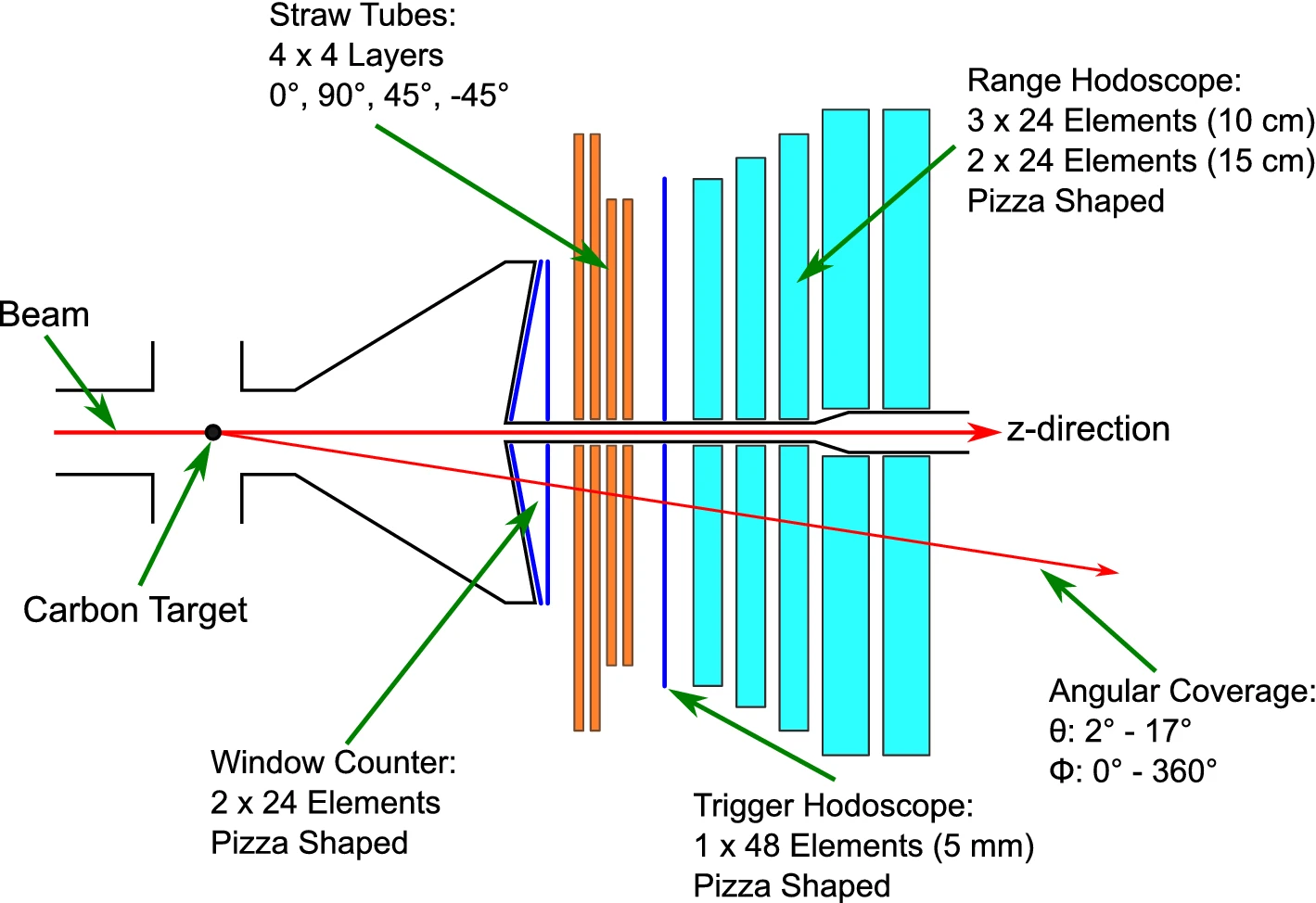
Figure 1: Cross sectional diagram showing the layout of the WASA Forward Detector, reprinted from [58]. The beam travels from left to right (horizontal red arrow), closely passing a 2-cm thick carbon block target along the way. The beam is heated vertically to bring beam particles to the front face of the target. Scattered particles moving forward exit the vacuum through a stainless steel window at angles between $2\mathrm{°}$ and $17\mathrm{°}$. They then pass through two plastic scintillator window counters cut into pie-shaped segments, an array of straw tubes for position and angle tracking, a segmented trigger hodoscope, and five layers (light blue) of plastic scintillator calorimeter detectors. The trigger counter and calorimeter detectors are also divided into pie-shaped segments. All the scintillator counters are read out using photomultiplier tubes mounted at the outer edge of each pie segment.

A 2-cm thick carbon block was inserted from above the beam and brought into position with the bottom edge aligned along the center of the WASA detector. This required that the beam be locally lowered by about 3 mm as it passed the carbon target. At the start of data acquisition, the beam was heated vertically using RF white noise generated in a band about one of the harmonics of the vertical tune. This brought beam particles to the front face of the target. From there, deuterons passed through the target. Some were scattered into the WASA detector system. The observed event rate was dominated by elastic scattering which has a forward-peaked angular distribution. The relevant analyzing powers for elastic scattering are shown in Ref. [58]. The detector acceptance was divided by software into four quadrants (left, right, down, and up). The sum of these four detector rates was fed back to control the power level of the white noise and maintain a constant event rate. Left-right and down-up asymmetries were computed in real time in four-second time intervals and made available for inspection as each beam store progressed. The down-up data stream was unfolded [59] based on the spin tune frequency in order to generate a value of the magnitude of the rotating in-plane component of the beam polarization.

A typical left-right asymmetry with the vertically polarized beam running was $0.12\pm 0.02$, where the error indicates the variation in this value during the experiment. This means that the cross section weighted average of the analyzing power over the WASA detector acceptance was $0.210\pm 0.035$.

The beam was accelerated in less than a second to full energy. Then electron cooling was applied for $71\text{\,}\mathrm{s}\text{/}$. This reduced the phase space of the beam to a point where the polarization lifetime in the horizontal plane could become long [51]. Once electron cooling was complete, the operating conditions for the beam were set. This required minimizing orbit deviations that would take the beam away from the centers of quadrupole lenses or having other unnecessary deviations. Finally, the polarization, which begins in the vertical direction, was rotated into the horizontal plane using an RF solenoid.

The timing list for a machine beam cycle is given in Table 1.

Table 1: Times for various COSY operations during the beam cycle

Event in the cycle	Time [s]
Acceleration off	0.674
E-cooling on	$4-75$
Carbon target moved in	75
White noise extraction on	77
WASA flag (DAQ on)	78
RF Solenoid on (rotate $p_{y}$)	$83-86$
Quick ramp to start of scan	$90.0-90.1$
Constant frequency hold	$90.1-120.1$
Ramp to search for ALP	$120.1-255.1$
Constant frequency hold	$255.1-285.1$
COSY RF stop	287
End of data taking	288

In order to precess the deuteron polarization into the ring plane, the RF solenoid was operated for $3\text{\,}\mathrm{s}$ on the $(1+G\gamma)f_{\mathrm{rev}}$ harmonic where $G=-0.1429873$ is the magnetic anomaly of the deuteron and $f_{\mathrm{rev}}=$750\,602.6\text{\,}\mathrm{Hz}\text{/}$$. At this frequency, the relativistic factor is $\gamma=1.126$. A search, made either as a scan or in fine steps, showed that the $(1+G\gamma)$ resonance for the RF solenoid occurred at $f_{\mathrm{sol}}=$629\,755.3\text{\,}\mathrm{Hz}\text{/}$$. The difference of these two frequencies, $f_{\mathrm{rev}}-f_{\mathrm{sol}}=$120\,847.3\text{\,}\mathrm{Hz}\text{/}$$, is the spin tune frequency, $f_{\mathrm{spin}}$. The frequency generators were synchronized with the $10\text{\,}\mathrm{MHz}\text{/}$ signal from GPS (Global Positioning System), thus the set values are precise and stable out to several mHz. From these two frequencies and the assumption that the COSY ring is purely magnetic, it is possible to deduce the kinematic parameters of the beam given in Table 2. This parameter list is shown without errors since they lie beyond the range shown in the table. The values are typical of the initial conditions of the deuteron beam in the storage ring before ramping. The setup of the Wien filter in Section II.3 contains the results of the scan used to determine the $(1-G\gamma)f_{\mathrm{rev}}$ spin resonance frequency. In that case the resonance shape was measured as part of the matching process and found to have a fractional full width of about $2\times 10^{-9}$ which represents one estimate of its precision.

Table 2: Beam parameters

Parameter	Symbol [Unit]	Value
Revolution frequency	$f_{\mathrm{rev}}$ [Hz]	$750602.6$
Spin resonance frequency	$f_{\mathrm{sol}}$ [Hz]	$629755.3$
Spin tune frequency	$f_{\mathrm{spin}}$ [Hz]	$120847.3$
Lorentz factor	$\gamma$ [1]	$1.126$
Beam velocity	$\beta$ [$c$]	$0.460$
Orbit circumference	$l$ [m]	$183.57$
Number of deuterons per cycle	$N_{d}$ [1]	$\approx 10^{9}$

As for the spin tune frequency $f_{\mathrm{spin}}$, the analysis of the polarization data allows us to measure it with a $10^{-10}$ precision [52], and the cycle-to-cycle variations are driven by the stability of the power supplies and the resulting orbit variations rather than by the precision of frequency setting.

It was important that the orbit does not deviate during the course of a ramp. This requirement was tracked with the use of beam position monitors (BPM).

The strategy for making the ALP search contained the steps shown in Fig. 2. Because of the necessity to maintain reproducible conditions for the rotation of the polarization from the vertical into the horizontal plane, all machine cycles began at the same beam energy or revolution frequency, as indicated by the blue horizontal axis in the figure. Once the polarization rotation was complete, a quick ramp was made to take the machine to the starting point for the scan. This removed the necessity to search for a new resonance frequency before every new scan. The scans, indicated by the long sloping lines in Fig. 2, lasted for $135\text{\,}\mathrm{s}\text{/}$. Before and after, there was a $30\text{\,}\mathrm{s}\text{/}$ period with no ramp. This was meant to provide extra data to characterize the starting and ending points under stable conditions. The ramps were planned to overlap at the ends, as shown in the figure. Since it was possible that an ALP-induced resonance might occur near the start or end, the overlap with the neighboring ramp was planned so that the resonance could be correctly characterized.

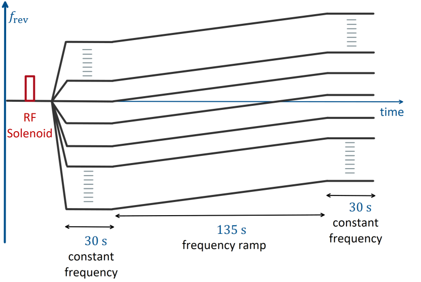
Figure 2: Diagram of revolution frequency as a function of time (black lines) showing how scans for axions were organized. The diagram includes an early time (marked in red) when the RF solenoid rotated the polarization into the horizontal plane. Then quick ramps took the machine to the start point for each ramp. Flat parts were included at the beginning and end of each scanning ramp to allow checks of the polarization with enhanced statistical precision. The resonance jump was expected to appear at some time during the frequency ramp.

Altogether, there were 103 ramps covering a range from $119.997\text{\,}\mathrm{kHz}\text{/}$ to $121.457\text{\,}\mathrm{kHz}\text{/}$, or an axion mass range of $4.955.02\text{\,}\mathrm{neV}\text{/}{\mathrm{\text{$c$}}}^{2}$.

In detail, after completing the initial preparatory phase of the machine cycle, the beam was brought to an interaction with the polarimeter target by moving the target into the correct position, turning on the RF white noise, and initiating the feedback used to maintain the polarimeter count rate. At this stage the data acquisition was turned on. After a short period that was used to check the vertical polarization, the RF solenoid was activated to rotate the polarization into the horizontal plane. For each scan, the machine was first set to the starting conditions. Then the first 30-s holding time took place, followed by the ramp and the second 30-s holding time.

The RF solenoid, whose magnetic axis is along the beam axis, operates by giving a series of small kicks to the rotation of the polarization. The magnetic field, except for some mild focusing effects, does not steer the beam. It thus maintains the constant orbit length constraint. The RF solenoid was kept running for $3\text{\,}\mathrm{s}\text{/}$. If allowed to continue, it would drive the vertical polarization into an oscillating pattern [60, 61]. The solenoid strength was adjusted until the vertical polarization component observed after the rotation was brought to zero. See the beginning of Appendix A for more details.

If the beam, once in the plane of the ring, remains polarized, then the down-up asymmetry in the WASA Forward Detector will oscillate with the precession frequency. However, this frequency is much too large to be able to observe even a single polarimeter event per oscillation, thus a different technique has been developed [52]. Namely, a value of the spin tune ($\nu=G\gamma$) was assumed and the data sorted among nine bins according to where the spin tune would predict it would lie along a single oscillation of the asymmetry. At the end of a preset time interval of $4\text{\,}\mathrm{s}$, the data accumulated in each of the time bins was used to calculate a down-up asymmetry for that bin. These asymmetries were reproduced with a sinusoidal curve from which the magnitude and phase of the oscillating horizontal asymmetry was obtained. The value of the spin tune was varied in small steps until a maximum in the amplitude of the sine wave was found [59]. The resulting magnitude and phase were recorded for that time bin. Data from the in-plane polarization measurement was recorded every $4\text{\,}\mathrm{s}$ in order to provide the statistics to complete this search. The processing time was quick enough that values of the horizontal asymmetry were made available in real time during the experiment.

The horizontal polarization is subject to depolarization because betatron oscillations of the beam particles lead to variations in their spin tunes. It has been shown that the addition of sextupole fields to the ring allow for the compensation of this depolarizing effect [51, 62]. Thus a part of the setup for this search involved optimizing these fields for the particular running conditions present in COSY at the time of this search. Online data was used to determine the horizontal polarization loss. Values for the strength of the three families of sextupole magnets were adjusted until the maximum polarization lifetime was obtained. During this experiment, the lifetime continued to vary because it was very sensitive to running conditions. At all times the slope of the horizontal polarization with time was maintained with a half-life greater than $300\text{\,}\mathrm{s}\text{/}$. Thus no more than a quarter of the polarization was lost during a typical scan.

II.1 Dealing with ALP Phase

During the scan, the phase of the oscillating EDM with respect to the rotating in-plane polarization (with reference to the beam-frame electric field) is not known. With only a single beam bunch in the machine at one time, the amplitude of a jump is modulated by a sine function of this relative phase. This situation could easily allow an ALP to be missed during a single scan. To avoid this, our strategy was to use more than one beam bunch at the same time since the same ALP phase is shared among all of these bunches. With the equipment available at COSY, bunching the beam up through harmonic 4 was already available.

A model study was performed to see if this change would satisfy the requirement with no further additions to the COSY ring. The details of this calculation are described in Appendix A. Assuming a round rather than a race-track shaped ring, it was found that four equally spaced bunches offered four mutually perpendicular orientations of the polarization direction relative to the beam-frame electric field (see Fig. 23). As the beam circulates in the ring, these four polarization directions rotate synchronously.

The COSY ring is race-track shaped, with arcs and straight sections of approximately the same length. This breaks the simple rotation pattern. Two bunches on opposite sides of the ring will have a rotating polarization while the two bunches in between will have a stationary phase without any electric field. This pattern swaps four times during each beam rotation. The sensitivity to all possible ALP phases comes from the comparison between neighboring bunches. During a single turn, the angle between polarization vectors of two subsequent bunches oscillates from $90\mathrm{°}$ to $61.2\mathrm{°}$ and back again. In this case, the actual sensitivity must be averaged over the range of angles covered in this oscillation. This results in a reduction of the signal by 4.2%, and the presented results have been corrected for this effect.

II.2 Scan Management

The approach to managing the scanning process was described in Section II above and is shown in Fig. 2. In preparing this scheme, one of the most crucial parts was the precession of the polarization from the vertical to the horizontal. To do this, the resonant frequency for the RF solenoid on a harmonic of the revolution frequency must be located experimentally to within about $0.1\text{\,}\mathrm{Hz}\text{/}$. This level of precision requires several tests that demonstrate an efficient precession process and the vanishing of the vertical polarization component at the end. This procedure is usually time consuming, taking longer than the series of scans themselves at one frequency setting. It was decided to separate the RF-solenoid-driven spin rotation from the rest of the scan procedure in order to save time and effort. After the RF-solenoid-driven spin precession was complete, the COSY operating frequency was ramped to the starting point for the scan and the scanning process began. In this way, the same resonance frequency is kept for all scans.

The ramping process itself must obey the constraint of preserving the orbit circumference while maintaining the optical properties of the beam. Even small variations can alter the way that sextupole corrections affect the beam. The resulting changes in the cancellation of depolarizing effects would make the lifetime of the horizontal polarization significantly smaller. For ramping, the two adjustable parameters on the machine are the magnetic field in the arcs and the frequency of the RF cavity that bunches (and accelerates) the beam. We chose to create a linear ramp in momentum. The field of the ring magnets is usually characterized by rigidity $B\rho$ which itself is proportional to the momentum. Thus, this requirement for the magnetic field is met straightforwardly using

$$B\rho=\frac{pc}{q},$$ (18)

where $\rho$ is the curvature radius of a particle track in field $B$, $c$ is the speed of light and $q$ is the electric charge of the nucleus. The bunching/accelerating cavity frequency must obey the same constraints and should follow

$$f_{\mathrm{rev}}=\frac{p}{\sqrt{m^{2}c^{4}+p^{2}c^{2}}}\frac{c}{\Lambda}\,,$$ (19)

where $m$ is the deuteron mass and $\Lambda$ is the orbit circumference. The value of $f_{\mathrm{rev}}$ used in the scan must be recalculated at each step of the ramp. The quality of the orbit control was checked by computing the RMS (Root Mean Square) deviation of the orbit summed over all of the beam position monitors in the ring. Control was adequate when this deviation was less than $1\text{\,}\mathrm{mm}\text{/}$.

The ramps were controlled by providing continuously changing momentum values to the COSY control system. The ramps were calculated from a common starting point of $970\text{\,}\mathrm{MeV}\text{/}\mathrm{\text{$c$}}$, the same momentum used for the RF solenoid on resonance. Then the machine settings were moved to the starting point for an ALP scan. Two speeds were employed during the experiment. For the faster ramps, the initial and final momenta were calculated according to

$$p_{0} = 970(1+1.173\times 10^{-4}n)\,$\text{\,}\mathrm{MeV}\text{/}\mathrm{\text{$c$}}$,$$ (20)

$$p_{f} = p_{0}+\Delta p,$$ (21)

where $n$ is the number of the scan (see Fig. 2), either positive or negative, away from $970\text{\,}\mathrm{MeV}\text{/}\mathrm{\text{$c$}}$ and $\Delta p$ is the momentum change in $135\text{\,}\mathrm{s}$. Table 3 gives the momentum change $\Delta p$ which was entered into the COSY control system and the corresponding change in $f_{\mathrm{spin}}$ and $f_{\mathrm{rev}}$ calculated from the read back from the RF cavity frequency. For the faster of the two ramps, the overlap between ramps was about $2.6\text{\,}\mathrm{Hz}\text{/}$.

For the slower ramps (second row), the same formula was used for $p_{0}$, but $\Delta p$ was decreased. In this case, there was a small coverage gap between adjacent ramps. The original plan was to have the ramps overlap so that resonances near the beginning or end of a scan would not be missed because of reduced time near the center of the resonance. As it is, they barely touched for the slow scans. There were 85 of the faster scans made with $n$ ranging from $-42$ to 42. For the 18 slow scans, $n$ ranged from $-60$ to $-43$.

Table 3: Change in beam parameters during the ramp

$\Delta p$ [$\text{\,}\mathrm{MeV}\text{/}\mathrm{\text{$c$}}$]	$\Delta f_{\mathrm{rev}}$ [$\text{\,}\mathrm{Hz}\text{/}$]	$\Delta\dot{f}_{\mathrm{rev}}$ [$\text{\,}\mathrm{Hz}\text{/}\mathrm{s}$]	$\Delta f_{\mathrm{spin}}$ [$\text{\,}\mathrm{Hz}\text{/}$]	$\Delta\dot{f}_{\mathrm{spin}}$ [$\text{\,}\mathrm{Hz}\text{/}\mathrm{s}$]
0.138	81.0	0.600	16.8	0.124
0.112	66.15	0.490	13.5	0.100

Each run usually consisted of ten separate beam fills. One out of five of the fills was deliberately unpolarized in order to provide a baseline for no polarization effect. Thus, each run usually consisted of eight polarized fills. The results from these fills were combined, as will be explained in more detail in the analysis section below, to yield sensitivity results for the range of the scan.

The goal for each fill was to begin with $10^{9}$ polarized deuterons. Due to changes in source and machine operation efficiency over time, this value could vary up or down by a factor of two. These changes are reflected in the final sensitivity as a function of ALP frequency.

The calibration of the jump size in terms of the size of the oscillating EDM is presented in Appendix B. Here in the description of the experiment, it is useful to illustrate an example of the signal as it might appear for one bunch during the experiment. This is shown in Fig. 3.

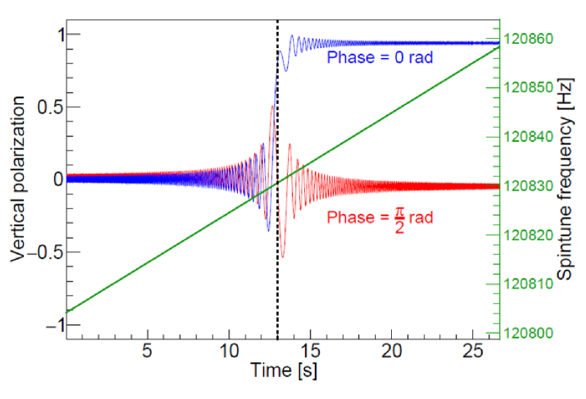
Figure 3: Graph of the vertical component of the polarization for a hypothetical resonance between the polarization rotation and the frequency of the ALP. Three quantities are shown as a function of time during a scan. The green line illustrates the changing spin precession frequency as time passes and the momentum of the beam is ramped up. At $13\text{\,}\mathrm{s}\text{/}$ the spin tune frequency and the ALP frequency in this model are the same. The blue and red curves show the time dependence of the vertical polarization component for two different choices of the ALP phase. In this case, initial conditions are such that a large jump is seen for a phase of zero and a much smaller, negative jump is seen for a phase of $\pi/2$. These two cases would sample the ALP phase along perpendicular axes, thus the sum in quadrature of the jumps would represent the strength of the ALP coupling to the deuteron.

In the analysis of the scans, the data were re-binned into 2-second bins, but the details of the resonance crossing as shown in Fig. 3, will not be apparent in the data. This same feature also applies to the Wien filter test described in the next Section. If the scanning speed is slower, then more time is available to make a polarization jump. Calibration calculations discussed in Appendix B show that the jump size scales as the square root of the reciprocal of the ramp rate.

II.3 Wien Filter Test

The COSY ring has been recently equipped with a spin manipulation tool that allows for spin rotations with minimal orbit disturbance, namely a waveguide RF Wien filter [63, 64, 65, 66]. It was especially designed for precision experiments including the measurements of permanent EDMs in a magnetic storage ring, which are performed at COSY in the framework of the JEDI collaboration. The electric field is generated in sync with a perpendicular magnetic field so that the beam orbit is not perturbed. The Wien filter can be rotated $90\mathrm{°}$ around the beam axis without breaking the vacuum to adjust the field directions to the experimental needs. We chose to use this device to test the ability of our system to detect a vertical polarization jump when passing a resonance. For this it was operated at a fixed frequency on the $(1-G\gamma)f_{\mathrm{rev}}$ resonance with the magnetic field horizontal, such that the polarization is rotated about a sideways axis. By scanning the Wien filter frequency in small steps, the resonant frequency was found to be $871450.039\pm 0.002$ Hz. The scan of the RF frequency was done in the way established for the ALP scans. In this setup, the phase between the Wien filter oscillation and the rotation of the in-plane polarization was arbitrary for each fill of the machine. Thus jumps were expected to be of variable sign and magnitude in consecutive cycles. Nevertheless, the result of a random distribution of phases should be a series of jumps between a positive and negative limit of the same size with more cases located near the limits (projection of a sinusoidal function on the $y$ axis). As was the case for the ALP scans, the ramp operated between $120\text{\,}\mathrm{s}\text{/}$ and $255\text{\,}\mathrm{s}\text{/}$ in the machine cycle, producing a ramping time of $135\text{\,}\mathrm{s}\text{/}$. Ramps were made with the resonance in the middle of the ramp. The ramps went in both directions. There were two different ramp speeds, based on a total momentum change of either 0.056 or $0.112\text{\,}\mathrm{MeV}\text{/}\mathrm{\text{$c$}}$ during the ramp.

As an initial calibration of the strength of the Wien filter magnetic field, beam injected with a vertical polarization (no RF solenoid) was subjected to continuous operation of the Wien filter from $88\text{\,}\mathrm{s}\text{/}$ to $285\text{\,}\mathrm{s}\text{/}$ in the machine cycle. Thus time that was normally not a part of the scan in the machine cycle was added to the time to observe oscillations. This extra time came mostly from the two 30-second periods used previously for the non-ramp data. This setup should produce a continuous oscillation of the vertical polarization component. Four different power levels were used for the Wien filter, each differing from the previous by a factor of two in magnetic field. In Fig. 4, data is shown between $81\text{\,}\mathrm{s}\text{/}$ and $287\text{\,}\mathrm{s}\text{/}$. The Wien filter is turned on at $t_{0}=$88\text{\,}\mathrm{s}\text{/}$$.

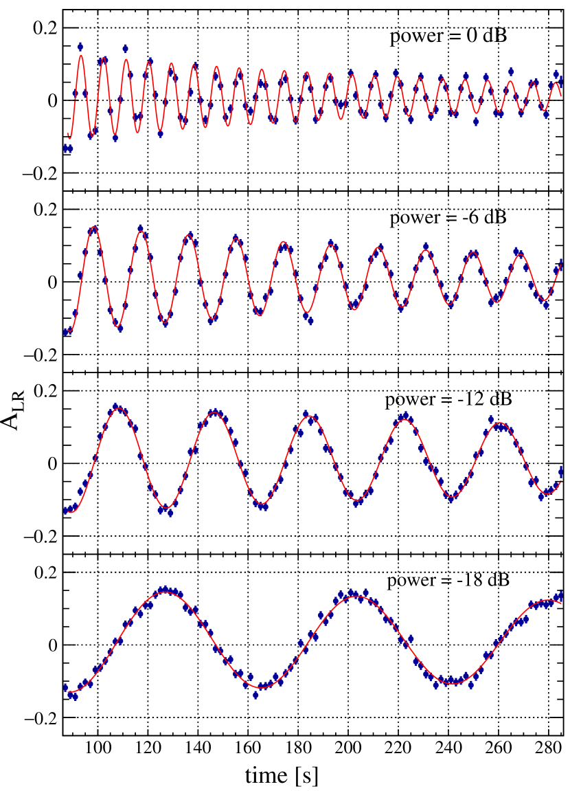
Figure 4: Measurements of the oscillating left-right asymmetry proportional to the vertical polarization produced by the continuous operation of the Wien filter at various power levels (noted in figure). The horizontal axis is time in seconds. The Wien filter was on continuously. Data from all four bunches were combined into a single asymmetry.

For the fits to the driven oscillations, the raw asymmetry data from the measurements were averaged across all four bunches and rebinned in 1-second intervals. Due to a slow depolarization arising from synchrotron oscillations [60], the oscillations are damped with time. These patterns were reproduced using the function

$$A_{\mathrm{LR}}(t)=A\left[e^{-\frac{t-t_{0}}{\tau}}\cos(2\pi f_{\mathrm{drv}}(t-t_{0})+\phi)\right]+k,$$ (22)

where $A_{\mathrm{LR}}(t)$ is the shape of the data, $A$ is the amplitude, $\tau$ is the decay constant, $f_{\mathrm{drv}}$ is the driven oscillation frequency, $\phi$ is the phase, and $k$ is the zero offset of the asymmetry data. The results for the frequency $f_{\mathrm{drv}}$, which is a measure of the strength of the Wien filter magnetic field, are given in Table 4. The right-hand column shows the ratio between the frequency on that row and the previous row. Given the power settings, this ratio should be two. Within a few percent, this ratio is realized. Variations are due to the properties of the control system of the Wien filter. When scans were recorded for the size of their jumps, a power level of 0 db was used.

Table 4: Driven oscillation frequencies. The third column contains the ratio of the current row frequency to the one of the preceding row.

Power (db)	Frequency (Hz)	Ratio
-18	0.013084(19)
-12	0.026326(21)	2.0122(33)
-6	0.052816(25)	2.0062(19)
0	0.110848(345)	2.0988(66)

III Data Analysis

The data available from each run consisted of the left-right asymmetry and the unfolded down-up asymmetry as functions of time before, during, and after each scan. These measurements were available from each of the four beam bunches. Since the initial vertical polarization has already been precessed into the ring plane, the left-right asymmetry where the jump may appear is initially close to zero. Meanwhile, the down-up asymmetry, which is subject to depolarization due to spin tune spread, declines slowly with time. This behavior was usually linear. For each fill and bunch, a linear fit to these data provided values of the in-plane asymmetry ($A_{\mathrm{IP}}$) as a function of time during the scan. Results from different bunches in the same fill were consistent. Jumps were observed only for the test case using the Wien filter to rotate the spins of the deuterons.

In line with the open science policy, the collected semi-raw experimental data have been made available in the Jülich DATA repository [67]. Two independent analyses have been performed using somewhat different analysis algorithms to define confidence intervals. As they yielded consistent results, in the following we present only one of the approaches based on the well-known Feldman-Cousins [68] procedure while the other can be found in [69].

Models, as described in the appendices, were used to relate the sizes of the jumps to the case where the beam polarization was unity and the effects were generated by the presence of an oscillating EDM. Subsequent examples of left-right asymmetries in this Section show the original measurements; any jumps recorded were then normalized by dividing by the linear fit to $A_{\mathrm{IP}}(t)$ appropriate for the time of the observation.

This Section addresses in turn the calculation of $A_{\mathrm{IP}}$ in the presence of ramping, the general treatment of possible jumps, and results for the Wien filter scans and the ALP scans. The jumps for the four bunches were then combined into a single result by fitting them to a sinusoid as a function of the relative phase between the beam rotation and the ALP oscillation. This process produces non-vanishing amplitudes for the sine wave even in cases where no effect is expected. This leads to a more complicated interpretation, as will be explained in Section III.5.

III.1 Calculation of the In-Plane Polarization

The analysis of the down-up in-plane asymmetry $A_{\mathrm{IP}}$ was described in Ref. [59]. Data consisting of down-up events were gathered into 2-second time bins. As a function of time the angle of the polarization $\alpha$ is given by

$$\alpha=\omega t=2\pi\nu f_{\mathrm{rev}}(t-t_{0})\,,$$ (23)

where the spin tune $\nu=G\gamma$ and the revolution frequency $f_{\mathrm{rev}}$ are assumed to be constant and $t$ is measured relative to $t_{0}$ at the beginning of the time bin. The events are divided into 12 angular bins according to the value of $\alpha$ modulo $2\pi$. The down-up asymmetry $A_{\rm DU}$ is calculated for the events in each bin. Finally, a sinusoidal curve is fit to $A_{\rm DU}(\alpha)$. The amplitude of the sine curve becomes the measure of $A_{\mathrm{IP}}$, the in-plane asymmetry. The phase of the fit is tracked as a function of time bin. A constant value is interpreted as a validation that the initial choice of spin tune is correct.

In the case of a scan, the spin tune undergoes a linear ramp from time $t_{1}$ to $t_{2}$, as depicted in Fig. 3. At the same time the machine revolution frequency also ramps. This gives

$$\centering\omega(t)=\begin{cases}2\pi\nu_{0}f_{\mathrm{rev,0}}\ \ \ \ \ \mathrm{for}\ t_{0}<t<t_{1},\\ 2\pi[\nu_{0}+\dot{\nu}(t-t_{1})][f_{\mathrm{rev,0}}+\dot{f}_{\mathrm{rev}}(t-t_{1})]\\ \ \ \ \ \ \ \ \ \ \ \ \ \ \ \ \ \ \ \mathrm{for}\ t_{1}<t<t_{2},\\ 2\pi\nu_{f}f_{\mathrm{rev,}f}\ \ \ \ \ \mathrm{for}\ t>t_{2},\end{cases}\@add@centering$$ (24)

$$\alpha(t)=\int_{t_{0}}^{t}\omega(t^{\prime})\mathrm{dt^{\prime}}$$ (25)

where the subscripts 0 and $f$ correspond to the initial and final values. Dotted symbols denote time derivatives. Once the spin phase $\alpha(t)$ is known, the calculation of $A_{\mathrm{IP}}$ proceeds as in the no-ramp case mentioned above.

III.2 Calculation of Polarization Jump

The data to be used in the analysis come from the left-right asymmetries recorded during the scanning process as a function of time. An illustration based on data taken with the Wien filter is shown in Fig. 5. With the level of time binning used in this experiment, the jump appears to be instantaneous. We represent this process using the step function:

$$f(t)=\begin{cases}{A_{\mathrm{LR}}}_{,0}&\mathrm{if}\ t<t_{\mathrm{step}},\\ {A_{\mathrm{LR}}}_{,0}+\Delta A_{\mathrm{LR}}&\mathrm{if}\ t\geq t_{\mathrm{step}}.\end{cases}$$ (26)

In this equation, ${A_{\mathrm{LR}}}_{,0}$ represents the left-right asymmetry before the scan as well as the asymmetry before the jump. The jump value, $\Delta A_{\mathrm{LR}}$, is the size of the change in the asymmetry. In Fig. 5, the black curve uses $t_{\mathrm{step}}$ = 187 s, the time when the in-plane polarization rotation frequency and the Wien filter frequency were the same. The step function is a good representation of these data.

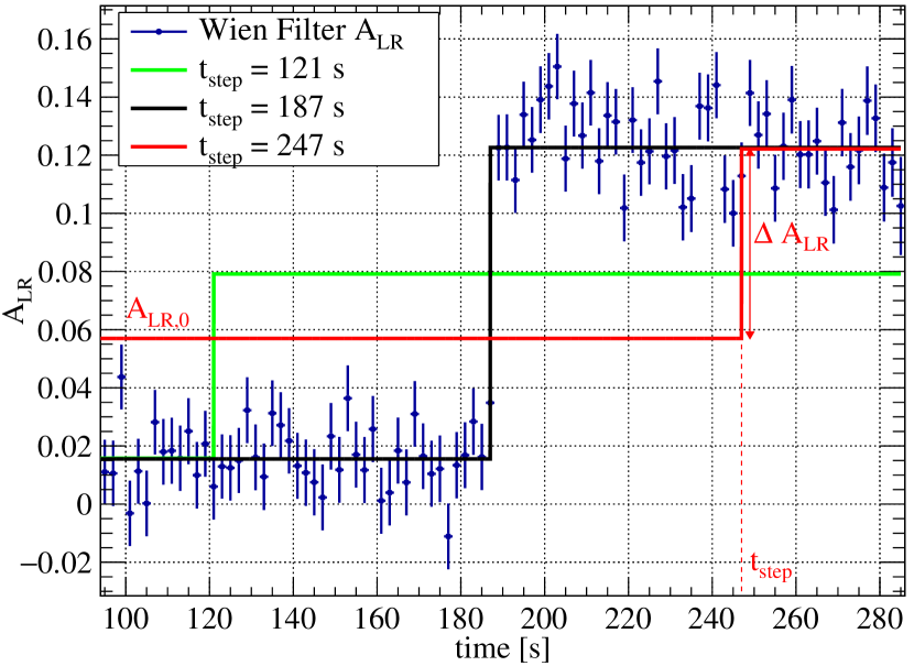
Figure 5: Examples of step function fits for the Wien filter scan data for a single bunch from one cycle. The black line is fit with the jump ($t_{\mathrm{step}}$) at the resonance crossing. The red and green curves show the results for other choices of the jump time. In both cases, the jump size is smaller and the reduced chi-square of the fit is increased (see Fig. 6).

In the case of normal scans for an ALP, we do not know a priori when the jump may have occurred, if at all. In this case, the fit is repeated as $t_{\mathrm{step}}$ is given the time of each bin from 121 to 257 s. When this is done for the Wien filter data of Fig. 5, the fits away from the resonance, as shown by sample red and green curves, display a smaller value of $\Delta A_{\mathrm{LR}}$. There is also a larger value of the fit $\chi^{2}$, as seen in Fig. 6 when $t_{\mathrm{step}}$ is away from the resonant frequency. Each cycle and bunch of the ALP search data was scanned for such a feature. The results will be discussed in Section III.4.

III.3 Wien Filter Scan Analysis

The Wien filter scan data consisted of 48 separate machine cycles. The four bunches within each cycle displayed oscillating jumps of the opposite sign. In each different cycle, the phase between the Wien filter and the rotating in-plane polarization was random. This resulted in variations in the jump size from cycle to cycle that spanned the range of possibilities. Statistical variations in the recorded asymmetries lead to errors in the jump of about 2%. In addition, the phase uncertainty multiplies this size by the cosine of the unknown relative phase. This acts to reduce all jump sizes. But the peak of the distribution should be close to the maximum value of one for the cosine.

To get a better estimate of the maximum, the absolute values of the jumps for the two ramp speeds were placed into separate distributions. In each case, there was a clear maximum. The jump amplitude was found by interpolating half way between the bin with the maximum number of cases in the upper 20% of the distribution and the maximum in the distribution. This in part allows the downward bias of the cosine effect to be corrected by the possible upward bias of the jump statistical distribution. An evaluation of this procedure using a Monte-Carlo model showed that the scatter of the answers was 2% given the number of jumps recorded, roughly the same as the statistical error in the jump size. The 2% error overlapped with the model value of the maximum jump.

The experimental values obtained using this procedure are presented in Table 5 along with the values from a dedicated simulation. This simulation was performed similarly to the one for the sensitivity calibration presented in Appendix B, only using the actual working parameters of the Wien filter and probing various relative phases. In addition, as the Wien filter is a localized device, the rotations have not been combined but executed subsequently as described for the RF solenoid simulation in Appendix A. The resonance strength of the Wien filter was derived from the ratio of the driven oscillation frequency (see Sect. II.3) to the revolution frequency in the storage ring at resonance

$$\epsilon_{\mathrm{WF}}=\frac{$0.110\,848\text{\,}\mathrm{Hz}\text{/}$}{$750\,602.6\text{\,}\mathrm{Hz}\text{/}$}=1.4768\times 10^{-7}\ .$$ (27)

This converts to an oscillation amplitude of the spin rotation per turn by the Wien filter of $\psi_{\mathrm{WF}}=4\pi\epsilon_{\mathrm{WF}}$ (see, e.g., Ref. [65]). Note that at this large resonance strength the linear dependence between rotation amplitude and polarization jump (see Appendix B) no longer holds and, thus, the ratio of the polarization signals for the two ramp rates does not reflect the discussed scaling behavior.

While neither pair of values agrees within errors, taken together there is a confirmation that the simulation program correctly models the sensitivity of the experiment. We will therefore assume that the calibration described in Appendix B may be used to determine our sensitivity to ALPs.

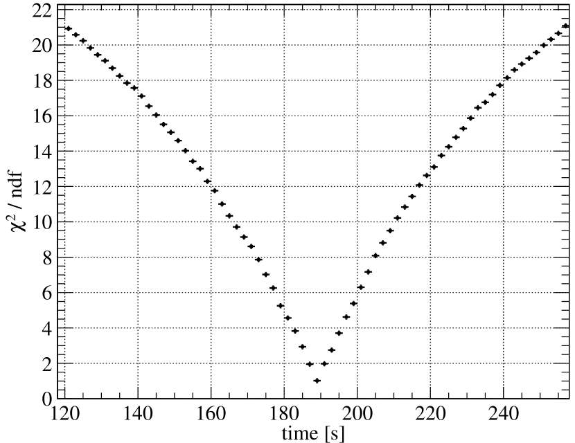
Figure 6: Reduced chi-squared plot of the step function fits for a Wien filter scan from one cycle as a function of the time assumed for the jump. The calculations are based on the data from Fig. 5. The minimum corresponds to the time when the resonance takes place.

Table 5: Comparison of the maximum polarization jump $\Delta p_{y}$ from simulation and experiment for the Wien filter test.

$\Delta p$ [$\text{\,}\mathrm{MeV}\text{/}\mathrm{\text{$c$}}$]	Simulation	Experiment
0.112	0.75	0.796(15)
0.056	0.93	0.892(18)

III.4 ALP Scan Analysis

For the data generated during scanning for an ALP, the process just described to locate the most probable time and size for a jump was repeated for each machine cycle and bunch. A typical example is shown in Fig. 7. Unlike the Wien filter case, there is no apparent jump. The red curve shows the largest possible jump found. This result is consistent with the lack of a minimum in the associated chi-square versus time plot presented in Fig. 8. Together, these results point to the absence of a resonance between the spin tune frequency and any ALP frequency within the range of the scan. The vertical bars in Fig. 8 indicate the standard deviation of the reduced $\chi^{2}$ distribution given by $\sqrt{2/\mbox{ndf}}$, where ndf indicates the number of degrees of freedom in the fit with ndf = $2\times 15$ flat region points + 68 scan region points $-$ 3 fit variables = 95. (This corresponds to a standard deviation of 0.145). Figs. 7 and 8 are for the scan data what Figs. 5 and 6 were for the Wien filter data.

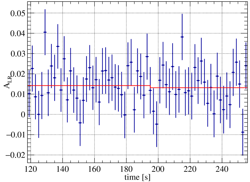
Figure 7: Example step function fit for an axion scan for a single bunch from one cycle. There is no jump in asymmetry since $\Delta{A_{\mathrm{LR}}}=-0.00105(233)$ is consistent with zero.

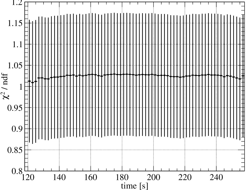
Figure 8: Reduced chi-squared plot of the step function fits for an axion scan from one cycle. The absence of a minimum indicates no resonance. The vertical bar shows the standard deviation of the chi square values based on the number of degrees of freedom.

To avoid missing an ALP due to a phase mismatch, the search results from all four bunches in each time bin of a scan were combined to produce a single sinusoidal curve as a function of possible phase using the formula

$$f(\phi_{m}) = C_{1}\sin{\phi_{m}}+C_{2}\cos{\phi_{m}},$$ (28)

$$\hat{A} = \sqrt{C_{1}^{2}+C_{2}^{2}},$$ (29)

where $m$ denotes the bunch number. The $y$-axis has been renormalized and shows the amplitude of each jump analysis divided by the in-plane asymmetry $A_{\mathrm{IP}}$ at the time of the tentative jump. The amplitude of the sinusoidal fit is given by Eq. (29). The spacing between the bunches on the $\phi_{m}$ axis is $\pi/2$ in Fig. 9. As was discussed at the end of Section II.1, the spacing is not always equal but oscillates between two extreme values. A correction is made for this effect.

The jump amplitude $\hat{A}$ (29) from the sinusoidal fit is calculated for each time bin and Fig. 10 shows the time distribution of that amplitude for one cycle. For multiple cycles covering the same frequency region, the mean amplitude is calculated for each time bin as a weighted average of amplitudes from the individual cycles. That mean and its uncertainty enter the next stage of the calculation of the confidence limit.

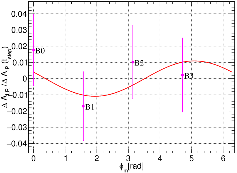
Figure 9: Left-right asymmetry jump for all four bunches, from one cycle, as a function of the angle between the bunch polarization and the axion phase $\phi_{m}$ for a single time bin. The red curve is the sinusoidal fit from which the jump amplitude $\hat{A}$ is calculated.

Figure 10: Amplitude $\hat{A}$ from sinusoidal fit for a single cycle.

III.5 Construction of Confidence Interval

The use of Eqs. (28) and (29) is designed to capture any possible ALP regardless of the ALP phase at the time of resonance crossing. The cost of using these equations is that near zero amplitude where most of the results will be, there is a systematic tendency to overestimate the size of the jump. Eq. (29) always generates a positive definite value. There is no distribution about zero that would allow zero as a mean. If $\hat{A}$ would happen to be large compared to its error, this effect would fade. To account for this positive bias and calculate a meaningful upper limit, the Feldman-Cousins procedure [68] will be used to construct the confidence interval. Refs. [70, 71] contain a detailed discussion on how the procedure is used for these cases.

In these references, the discussion describes how to interpret the estimated amplitude ($\hat{A}$) in terms of a true amplitude ($A$). In order to facilitate the application to a large number of time bins as a function of ALP frequency, we will switch to the amplitude normalized by the statistical error. This gives the normalized estimated value ($\hat{P}=\hat{A}/\sigma_{\mathrm{exp}}$) and true value ($P=A/\sigma_{\mathrm{exp}}$). The advantage is that we do not need to regenerate the interpretation for each time bin.

The probability density function (PDF) for data distributed according to $\hat{A}=\sqrt{{C}_{1}^{2}+{C}_{2}^{2}}$ is given in Eq. (2.2) of [71]. Modifying this for the $P$ quantity we obtain:

$$f(\hat{P}|P)\,\mathrm{d}\hat{P}=e^{-\frac{\hat{P}^{2}+P^{2}}{2}}\hat{P}I_{0}(\hat{P}P)\,\mathrm{d}\hat{P},$$ (30)

where $I_{0}$ is the modified Bessel function of the first kind. Equation (30) is called the Rice distribution. A 2-dimensional graphical representation of this distribution for $0\leq P\leq 6$ is shown in Fig. 11. The red line denotes $P_{\mathrm{best}}$, which is the value of $P$ for which $f(\hat{P}|P)$ has the maximum probability in the physically allowed region for $P$.

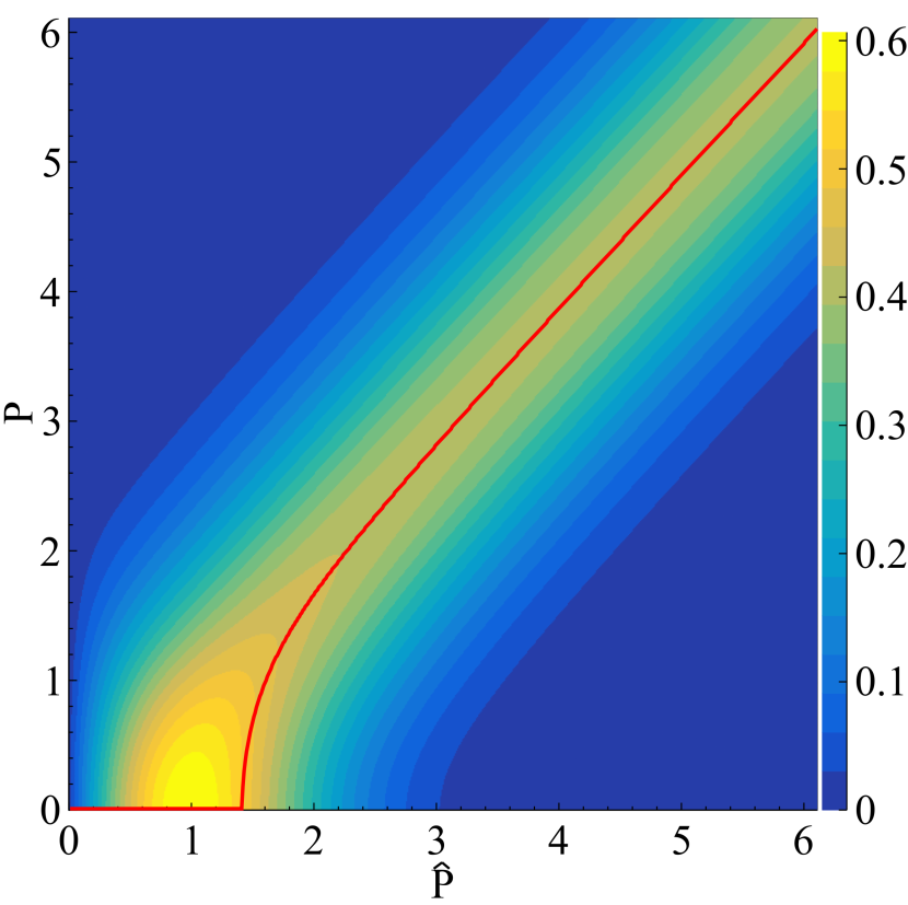
Figure 11: A 2-dimensional Rice plot for one cycle. The red line represents the value of $P$ for which the Eq. (30) is maximum for a given value of $\hat{P}$.

The distortion of the distribution away from a typical Gaussian shape where $P\approx\hat{P}$ becomes clear below $\hat{P}=2.5$. For quantities that are near zero, the estimated or experimental value is about one. This means that the experiment seems to produce evidence of an effect even though it is only significant at the one standard deviation statistical level.

Next a likelihood ratio $R$ is calculated using the following definition,

$$R=\frac{f(\hat{P}|P)}{f(\hat{P}|P_{\mathrm{best}})}.$$ (31)

Two examples of the likelihood curve for $P=1.0$ and 2.8 are shown, in blue, in the top row of Fig. 12. The Feldman-Cousins confidence interval is constructed by determining the bounds within which the integral of $f(\hat{P}|P)$ reaches the desired confidence interval, e.g., 90%. The bottom row of Fig. 12 shows the PDF for $P=1.0$ and 2.8 along with the gray shaded region denoting the 90% confidence limit for the two cases above.

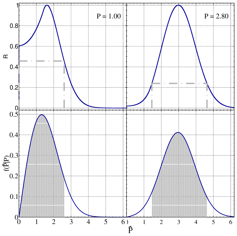
Figure 12: Two examples, left $P=1.0$ and right $P=2.8$, for the calculation of 90% confidence limits using the likelihood ratio given by Eq. (31) (top row) and PDF given by Eq. (30) (bottom row). The gray horizontal dashed line in the likelihood ratio curves denote the $R$ value for which the corresponding $\hat{P}$ values (gray vertical dashed lines) forms the 90% integral in the PDF curves. The gray shaded region marks the 90% integral region.

The confidence limit bounds on $\hat{P}$ are determined by starting with the largest value of $R$ where it is one and following the two limit points given by the intersection of a straight horizontal line with the likelihood ratio curve as the line moves down the plot. In the upper left case where the curve ends at $\hat{P}=0$ as the horizontal line crosses $R=0.6$, the left axis where $\hat{P}=0$ replaces the lower limit of the $R$ curve. This process continues until the integral (gray shading) of the lower curve between the two limits reaches the desired confidence level. For the right-hand “Gaussian” case, both limits are still on the $R$ curve and are roughly symmetric about the peak of $R$. The lower and upper limits of $\sim\!1.5$ and $\sim\!4.6$ represent the bounds of the 90% confidence interval. For the “left-hand” case there is only an upper limit at $\sim\!2.6$. Most of the data points in this experiment follow this example.

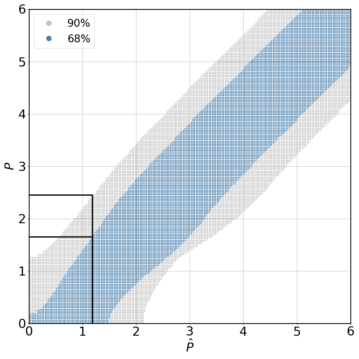
Figure 13: A 68% (blue) and 90% (gray) confidence interval for one cycle analysis. On the $x$-axis we have the estimated value $\hat{P}$ and on the $y$-axis is the true value $P$.

A summary of all of the limits for $P$ may be found in Fig. 13. Inside the blue band the confidence is 68%. The gray band outside the blue band shows the edges for the 90% limit. For a given value of $\hat{P}$ trace a line upward until it crosses the appropriate boundary. The case shown is for an upper limit only where there is no lower limit other than zero. These limits correspond to a single beam fill in the experiment with only one scan.

Since most scans comprise 8 cycles the confidence interval needs to be constructed taking this into account. A few scans comprised 7, 9, or 16 cycles. According to the central limit theorem, for $n$ cycles $\hat{P}$ follows a Gaussian distribution, the mean amplitude remains at the same $A$ value and the uncertainty is $\sigma_{n}=\sigma_{\mathrm{exp}}/\sqrt{n}$. It is assumed that this is approximately true since, once set up, the beam current reproduced well from cycle to cycle for any particular scan. All $\sigma_{\mathrm{exp}}$ are the same for cycles being averaged this way. The PDF for $n$ cycles is a Gaussian with $P=A/\sigma_{n}$:

$$f(\hat{P}|P) = \frac{1}{\sqrt{2\pi}\sigma_{\mathrm{Rice}}}e^{\frac{(\hat{P}-\mu_{\mathrm{Rice}})^{2}}{2\sigma^{2}_{\mathrm{Rice}}}},$$ (32)

$$\mu_{\mathrm{Rice}} = \sqrt{\frac{\pi}{2}}\sqrt{n}L_{1/2}\left(-\frac{1}{2}\frac{P^{2}}{n}\right),$$ (33)

$$\sigma^{2}_{\mathrm{Rice}} = 2+\frac{P^{2}}{n}-\frac{\pi}{2}L^{2}_{1/2}\left(-\frac{1}{2}\frac{P^{2}}{n}\right),$$ (34)

where $L_{1/2}$ is the Laguerre polynomial.

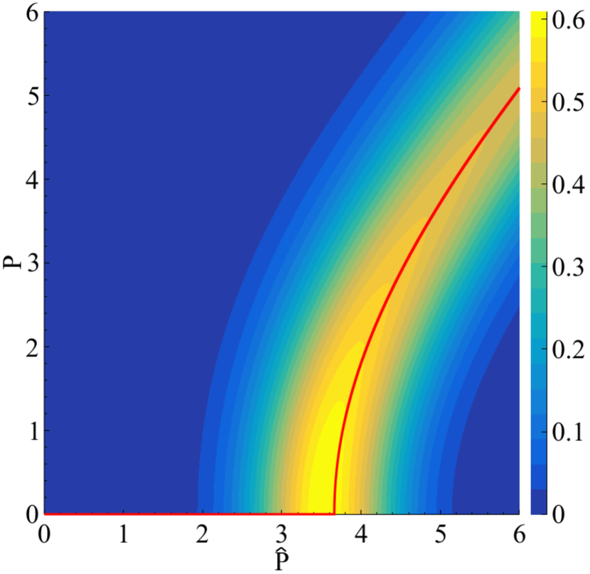
Figure 14: A 2-dimensional Rice plot for 8 cycles. The red line represents the value of $P$ for which the Eq. (32) is maximum for a given value of $\hat{P}$.

Figure 14 is the 2-dimensional plot for $n=8$ calculated using Eq. (32). The construction of confidence interval follows the 1 cycle case. The confidence interval for $n=8$ is shown in Fig. 15. The edges of the blue and gray bands represent the 68% and 90% confidence levels, respectively.

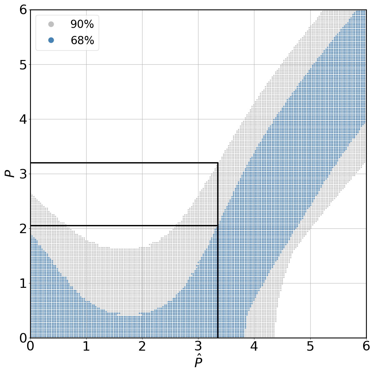
Figure 15: A 68% (blue) and 90% (gray) confidence interval for the multi-cycle analysis $(n=8)$. On the $x$-axis we have the estimated experimental value $\hat{P}$ and on $y$-axis is the true value $P$. For an experimental value of $\hat{P}=3.3$, the true value $P$ can be found between 0 and 3.15 with a confidence of 90%.

Care must be taken if the observed $\hat{P}$ is less than the expected value $\mu_{\mathrm{Rice}}$. These are considered to be from downward statistical fluctuations and $P$ is calculated at $\mu_{\mathrm{Rice}}$ as explained in [68]. For each experimentally obtained value of $\hat{P}$ the corresponding boundary values of $P$ are determined. This value is multiplied by the experimental uncertainty $\sigma_{n}$ to give the true amplitude $A$. In the frequency range or axion mass range covered by the experiment, no signal was observed that could not be explained by a statistical fluctuation. Note that in setting a 90% confidence interval, one expects that in 10% of the cases a lower limit larger than zero even if no signal is present. This corresponds to our observation, as shown in Fig. 16. From this we also conclude that at this level of precision there is no systematic effect resulting in a fake signal.

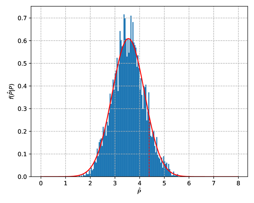
Figure 16: The blue histogram is the distribution of $\hat{P}$, normalized such that the integral is one. The experimental data is in good agreement with the probability density function for $P=0$ (Eq. (32)) drawn in red. In both cases there are $n=8$ cycles. The vertical red line at $\hat{P}=4.38$ corresponds to the lower limit of the 90% confidence interval being greater than zero. This is the case for 9.63% of the contributing data points.

The conversion into a limit of the oscillating EDM of the deuteron is done through the equation:

$$|d_{\mathrm{AC}}^{d}|=\lambda A\times 10^{-23}~{}\!$\text{\,}\mathrm{\text{{\hbox{e}}}}\text{\,}\mathrm{cm}\text{/}$,$$ (35)

where here and in the following we use the convention that the unit of electric charge $e$ is defined to be positive. The coefficient $\lambda=316$ for the fast ramps and $286$ for the slow ramps, respectively. $\lambda$ is based on a model of the polarization jump size for a particular ramp rate. The derivation of Eq. (35) is given in Appendix B, see Eq. (53).

IV Result and Discussion

IV.1 Limits of ALPs signals

According to references [44, 45] the angular velocity $\vec{\Omega}$ of the extended Thomas-BMT equation (12) of a beam with particles of mass $m$, charge $q$, spin $S$, Lorentz factor $\gamma$ and velocity $\vec{v}=c\vec{\beta}$ acquires the following oscillating term

$$\vec{\Omega}_{a(t)} = -\frac{1}{S\hbar}\,\frac{d_{\mathrm{AC}}}{a_{0}}\,a(t)\,c\vec{\beta}\times\vec{B}-\frac{1}{S\hbar}\,\frac{C_{N}}{2f_{a}}\,\hbar\partial_{0}a(t)\,\vec{\beta}$$ (36)

$$= \phantom{-}d_{\mathrm{AC}}\frac{c\gamma m}{q\hbar S}\cos\big{(}\omega_{a}(t-t_{0})+\phi_{a}(t_{0})\big{)}\,\vec{\beta}\times\vec{\Omega}_{\mathrm{rev}}$$

$$\mbox{}+\frac{C_{N}}{2f_{a}S}\omega_{a}a_{0}\sin\big{(}\omega_{a}(t-t_{0})+\phi_{a}(t_{0})\big{)}\,\vec{\beta}\,,$$

whenever a classical ALP field, as in Eq. (3), couples to the particles stored in the beam, cf. Eqs. (8) to (11). Note that the magnetic field in the laboratory system can be expressed as $\vec{B}=(-m\gamma/q)\vec{\Omega}_{\mathrm{rev}}$ in terms of the angular revolution velocity of the particle beam, $\vec{\Omega}_{\mathrm{rev}}$, as shown in Eq. (14).

According to Eq. (36) the spin rotation around the axis $\vec{\beta}\times\vec{\Omega}_{\mathrm{rev}}$ (the latter always points radially outward, regardless of whether the beam is rotating clockwise or counterclockwise) is generated by the AC part of the electric dipole moment of the beam particle (see Eq. (7)) which in turn is induced by the ALP field, while the spin rotation with respect to the longitudinal axis $\vec{\beta}$ of the beam, see [44, 45], follows from the pseudomagnetic (axion-wind) effect [39, 18] of strength $C_{N}/f_{a}$ in terms of the axion decay constant $f_{a}$ [12]. In the experiment we cannot distinguish these two rotation types around two orthogonal axes which both induce – on resonance – a polarization shift in the vertical direction but are $\pi/2$ out of phase with each other, so that the two rotation amplitudes add up coherently.

Thus, to obtain an upper limit on $d_{\mathrm{AC}}$ or $C_{N}/f_{a}$ one has to assume that the other term vanishes, such that the bound is saturated by one term only.

First we assume that only the EDM-term is present, i.e., $C_{N}/f_{a}=0$. Figure 17 provides the 90% confidence level sensitivity for excluding the ALPs induced oscillating EDM of the deuteron, $d_{\mathrm{AC}}^{d}$, in the frequency range of $120.0121.4\text{\,}\mathrm{kHz}\text{/}$ and the corresponding axion mass range of $0.4950.502\text{\,}\mathrm{neV}\text{/}{\mathrm{\text{$c$}}}^{2}$ represented on the upper axis. The darker lines indicate the upper limit of the oscillating EDM and the lighter filled region above is the exclusion region. The green and blue colors differentiate the two different ramp rates mentioned in Section II.2. The green indicates a momentum change $\Delta p=$0.112\text{\,}\mathrm{MeV}\text{/}\mathrm{\text{$c$}}$$ and the blue $\Delta p=$0.138\text{\,}\mathrm{MeV}\text{/}\mathrm{\text{$c$}}$$.

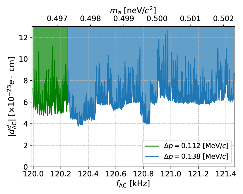
Figure 17: 90% confidence level sensitivity for excluding the ALPs induced oscillating EDM ($\text{\,}\mathrm{\text{$e$}}\text{\,}\mathrm{cm}\text{/}$) in the frequency range $120.0121.4\text{\,}\mathrm{kHz}\text{/}$ ($m_{a}=$ $0.4950.502\text{\,}\mathrm{neV}\text{/}{\mathrm{\text{$c$}}}^{2}$). More explanation may be found in the text.

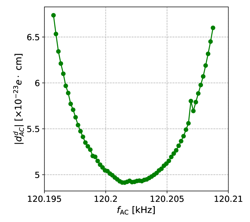
Figure 18: Sensitivity of a single scan including 8 cycles. The sensitivity decreases and the curve gets larger as one moves away from the center of the scan. There is no overlap between the scans in this example.

The fluctuations in the exclusion plot result mainly from two beam properties, intensity and polarization, as well as the clock time during the scan. Good beam properties mean better sensitivity. The dependency of intensity is seen in a larger scale over multiple scans. If for a particular frequency range, a larger number of scans were performed, the obtained sensitivity is better. This can be observed in Fig. 17 around frequency $120.8\text{\,}\mathrm{kHz}\text{/}$, for example. The decline in sensitivity within a cycle is mainly due to beam depolarization.

A small contribution to these fluctuations arises from the way $\Delta{A_{\mathrm{LR}}}$ is calculated in Eq. (26). As a consequence, the sensitivity becomes worse as one moves further from the middle of the scan because the imbalance in the number of points on both sides of the anticipated jump in the calculation of $\Delta{A_{\mathrm{LR}}}$ leads to a larger uncertainty in the jump. An example of how this sensitivity appears for a single scan region comprising 8 cycles is shown in Fig. 18. However, the intensity of the beam and the polarization have the greatest influence and their combination is the reason for the higher values ($|d_{\mathrm{AC}}^{d}|>$8\text{\times}{10}^{-23}\text{\,}\mathrm{\text{$e$}}\text{\,}\mathrm{cm}\text{/}$$).

This experiment to search for ALPs in the storage ring provides a 90% confidence level upper bound of

$$|d_{\mathrm{AC}}^{d}|<$6.4\text{\times}{10}^{-23}\text{\,}\mathrm{\text{{\hbox{e}}}}\text{\,}\mathrm{cm}\text{/}$.$$ (37)

This value is used to calculate ALP coupling constants in the next subsection and is based on the average of the individual limit points in Fig. 17.

IV.2 Limits of Various ALP Couplings

In this paper, we focus on the coupling of ALPs to the deuteron spin via the oscillating part of the deuteron EDM $d_{\mathrm{AC}}^{d}$ and/or via the axion wind effect proportional to $C_{d}/f_{a}$. For all these calculations, it is assumed that the local dark-matter density $\rho_{\mathrm{LDM}}=(0.55\pm 0.17)\,$\text{\,}\mathrm{GeV}\text{/}{\mathrm{cm}}^{3}$$ (see, e.g., Chapter 27 “Dark Matter” of Ref. [12]) contains only ALPs.

The bound on the amplitude of the oscillating deuteron EDM $d_{\mathrm{AC}}^{d}$, cf. Eq. (37), can be interpreted as a bound on the axion coupling to the deuteron EDM operator (in analogy to the axion coupling to the nucleon EDM operator, $g_{aN\gamma}$, of [12, Eq. 90.38], see also Eqs. (8) and (9)) in terms of the electromagnetic fine-structure constant $\alpha$:

$$|g_{ad\gamma}|=\frac{|d_{\mathrm{AC}}^{d}|}{a_{0}}\,\frac{\sqrt{4\pi\alpha}}{e\hbar c}<$1.7\text{\times}{10}^{-7}\text{\,}{\mathrm{GeV}}^{-2}$.$$ (38)

Here we assume that $a_{0}=\sqrt{2\rho_{\mathrm{LDM}}(\hbar c)^{3}}/(m_{a}c^{2})=$5.8\text{\,}\mathrm{M}\mathrm{e}\mathrm{V}$$. The occurrence of the axion/ALP amplitude $a_{0}$ in the denominator of Eq. (38) is typical when the calculation is based on axion/ALPs as candidates for (local) dark matter particles. The inverse proportionality of $a_{0}$ and $m_{a}$ implies that the exclusion limits derived from oscillating EDM measurements at similar experimental sensitivity have to be linearly increasing functions of the ALP mass $m_{a}$.

Figure 19 shows the limit on |$g_{ad\gamma}$| from this experiment in cyan along with bounds for $|g_{aN\gamma}|$ from the nEDM [25], CASPEr-electric [72], and Beam EDM [73] experiments. In addition, the figure presents the $|g_{aN\gamma}|$ exclusion region as tabulated in [74] via reformulating the limits of the electron-EDM HfF⁺ experiment [26, Fig. 3]. Furthermore, a constraint on $|g_{aN\gamma}|$ is shown that is derived in Ref. [18] from assuming $N+\gamma\to N+a$ cooling in SN1987A. Thus the latter bound is based on the strength of the coupling constant in the axion/ALP interaction with the nucleon EDM and is therefore independent of $m_{a}$. Note, however, that Ref. [75] suggests an alternative collapse mechanism for supernovae SN1987A that would not place limits on the emission of ALPs or axions. Moreover, following Ref. [74], an exclusion region is shown that is based on a new constraint on the coupling of thermally-produced ALPs as calculated in Ref. [76] from combined data of cosmic microwave background spectra and baryon acoustic oscillations. However, according to [76] these bounds were only derived for the mass range $10^{-4}$\text{\,}\mathrm{e}\mathrm{V}\mathrm{/}\mathrm{c}^{2}$\lesssim m_{a}\lesssim$100\text{\,}\mathrm{e}\mathrm{V}\mathrm{/}\mathrm{c}^{2}$$. Our directly measured upper bound (38) at $m_{a}=$0.5\text{\,}\mathrm{neV}\text{/}{\mathrm{\text{$c$}}}^{2}$$ falls within the model-dependent constraint obtained from SN1987A, but is stronger than the CASPEr-electric result at $m_{a}\approx$100\text{\,}\mathrm{neV}\text{/}{\mathrm{\text{$c$}}}^{2}$$.

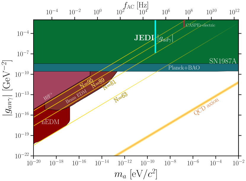
Figure 19: The 90% upper bound on |$g_{ad\gamma}$| from this experiment (in cyan) is shown along with the bound on |$g_{an\gamma}$| from experiments such as nEDM [25], CASPEr-electric [72], HfF⁺ [26], and Beam EDM [73] (as presented in Ref. [74]), in different shades of red. Also, seen in green is the constraint, calculated in [18] from the SN1987A supernova energy loss, which might be model-dependent [75]. In blue a further constraint calculated in [76] from the combined Planck 2018 and BAO (baryon acoustic oscillation) cosmological data is displayed (as presented in Ref. [74]). Finally, the yellow lines $\mathcal{N}=n$, parallel to the QCD axion band and plotted according to Eq. (2) and Eq. (90.5) of [12], indicate that $Z_{\mathcal{N}}$ axions with $\mathcal{N}>n$ are excluded by the above-mentioned measured bounds in their respective mass ranges. Figure courtesy [74, 12].

Finally, in Figure 19, $|g_{an\gamma}(m_{a})|_{\mathcal{N}}$ lines of the $Z_{\mathcal{N}}$-axion model are plotted which follow from the exclusion limits of the presented EDM-based experiments and which run parallel to the displayed QCD axion band. Each $\mathcal{N}$ must be an odd-valued positive integer as otherwise the pertinent model would not solve the strong CP problem, see [13, 14], and one would be back at the ALP case. In detail, according to Eq. (2) combined with Eq. (90.5) of [12], i.e.,

$$g_{an\gamma}=(3.7\pm 1.5)\times 10^{-3}\,{\rm GeV}\,\frac{1}{f_{a}(m_{a})|_{\mathcal{N}}}\,,$$ (39)

$Z_{\mathcal{N}}$ axions with $\mathcal{N}>81$ are excluded by our bound (38) at $m_{a}\simeq$5\text{\times}{10}^{-10}\text{\,}\mathrm{e}\mathrm{V}\mathrm{/}\mathrm{c}^{2}$$. Even if the canonical QCD axion/ALPs scenario prevails, the straight lines (proportional to $m_{a}$) that can be derived from Eq. (39) can still serve as excellent guides for “extrapolating” exclusion limits to different ALP masses and therefore comparing the experimental sensitivities of the underlying measurements of hadron (neutron, proton, deuteron, etc.) electric dipole moments. For instance, the line $\mathcal{N}=63$ shows that the pertinent experimental sensitivity of the nEDM limits is approximately a factor $10^{3}$ better than in our experiment. This is compatible with a factor $\sim 10^{-3}$ between the oscillating neutron EDM bounds between $5.0\text{\times}{10}^{-26}\text{\,}\mathrm{\text{$e$}}\text{\,}\mathrm{cm}\text{/}$ to $7.0\text{\times}{10}^{-26}\text{\,}\mathrm{\text{$e$}}\text{\,}\mathrm{cm}\text{/}$ as shown in [25, Fig. 2] and our upper bound $|d_{\mathrm{AC}}^{d}|<$6.4\text{\times}{10}^{-23}\text{\,}\mathrm{\text{$e$}}\text{\,}\mathrm{cm}\text{/}$$, see Eq. (37). The line $\mathcal{N}=89$ indicates that the CASPEr-electric limit [72] is roughly a factor 20 less sensitive than that of our experiment, while the sensitivity of the Beam EDM experiment [73] is slightly better than ours. Finally the HfF⁺ limits [26] exclude $Z_{\mathcal{N}}$ axions with $\mathcal{N}>95$ in the specified mass range. The corresponding $\mathcal{N}=95$ line implies that the sensitivity of this electron-EDM based experiment to constrain oscillating hadronic EDMs is about $10^{2}$ times worse than in our case.

The second coupling we considered is the ALP-gluon coupling $C_{G}/f_{a}$, generated from the $\bar{\Theta}$ term for the permanent EDM case, where the use of $C_{G}/f_{a}$ instead of just $1/f_{a}$ takes into account that the ALP coupling strength might differ from the axion one. The coupling is given by [17, 77, 25]

$$d_{\mathrm{AC}}^{N}(t)=S\cdot\kappa_{a}\frac{e\hbar c}{2mc^{2}}\cdot\frac{C_{G}}{f_{a}}\cdot a_{0}\cos\left(\omega_{a}(t-t_{0})+\phi_{a}(t_{0})\right)$$

$$\approx$2.4\text{\times}{10}^{-16}\text{\,}\mathrm{\text{$e$}}\text{\,}\mathrm{cm}\text{/}$\cdot\frac{C_{G}}{f_{a}}\cdot a_{0}\cos\left(\omega_{a}(t-t_{0})+\phi_{a}(t_{0})\right),$$

where $S$ and $m$ are the spin and mass of the nucleon, respectively, and $\kappa_{a}$ is the chiral suppression factor of the $\bar{\Theta}$-term. Here the loop-enhanced value $\kappa_{a}\approx 0.046$ of [77, 12, 25] was used. Note that the numerical factor $2.4\text{\times}{10}^{-16}\text{\,}\mathrm{\text{$e$}}\text{\,}\mathrm{cm}\text{/}$ is the same for proton (or neutron) and deuteron because the ratio $S/m=(1/2)/m_{p}\approx 1/m_{d}$ is approximately the same for these particle species. Compared to the direct determination of $C_{G}/f_{a}$ in the case of the nucleon, however, corrections are expected in the deuteron scenario. From the isoscalar nature of the deuteron nucleus and the isovector nature of the leading low-energy pion-loop contribution to the nucleon EDM [78, 79, 80], a severe cancellation between the contributions of its proton and neutron components is anticipated, see e.g., Ref. [12]. Moreover, the small $D$-wave admixture of the deuteron wave function affects the weights of these individual nucleon components [81, 82]. Finally $P$- and $T$-breaking meson-exchange terms contribute already at leading tree-level order [83, 84]. The latter contributions to the permanent EDM of the deuteron, induced by the QCD-theta term or more generalized chromo-electric EDMs of quarks, are shown to be of similar magnitude as the single nucleon ones, see, e.g., [81, 82, 83, 84, 85, 86, 87, 88, 89, 90]. The ALP-gluon coupling in the deuteron case is therefore denoted in the following by an upper index $d$, i.e., $C_{G}^{d}$, to signal that this coefficient is likely to contain corrections of order one relative to the coupling $C_{G}$ in the nucleon scenario.

So substituting $S=1$ and $m_{d}$ for the deuteron, we get the bound on the coupling constant,

$$\left|\frac{C_{G}^{d}}{f_{a}}\right| = \left|\frac{d_{\mathrm{AC}}^{d}}{$2.4\text{\times}{10}^{-16}\text{\,}\mathrm{\text{$e$}}\text{\,}\mathrm{cm}\text{/}$\times a_{0}}\right|$$ (41)

$$< $0.46\text{\times}{10}^{-4}\text{\,}{\mathrm{GeV}}^{-1}$.$$

Note again the $a_{0}$ dependence in the denominator which implies a linear dependence of the bound on ALP mass $m_{a}$ and is a signal that the calculation is based on axions/ALPs as dark-matter candidates.

Figure 20 shows the upper bound on $|\frac{C_{G}^{d}}{f_{a}}|$ in comparison with the results on $|\frac{C_{G}}{f_{a}}|$ from the nEDM experiment [25], the HfF⁺ electron EDM [26] and the Beam EDM [73] experiments as well as the limits obtained from astrophysical calculations such as Big Bang nucleosynthesis, solar core, and supernova SN1987A [18] – the latter based on the $N+\gamma\to N+a$ cooling mechanism. Details can be found in [12, 74]. Our result is within the limits obtained from the supernova emission. In addition, three $Z_{\mathcal{N}}$ lines are plotted, given directly by $1/f_{a}(m_{a},\mathcal{N})$, as calculated in Eq. (2). They show that $Z_{\mathcal{N}}$ axions with $\mathcal{N}>81$ and $\mathcal{N}>63$ are again excluded by the JEDI and nEDM [25] experiments in their respective mass regions, while the eEDM-based HfF⁺ exclusion region, see Ref. [26], vetoes $Z_{\mathcal{N}}$ axions with $N>95$ in the specified mass range. Note that the apparently better fitting line $\mathcal{N}=96$ can be excluded for another reason, since $Z_{\mathcal{N}}$ axions with even $\mathcal{N}$ do not solve the strong CP problem.

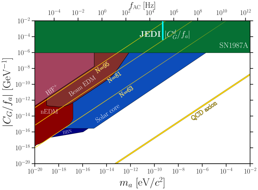
Figure 20: Figure showing the 90% upper bound on $|{C_{G}^{d}}/{f_{a}}|$, in cyan, in comparison with the $|C_{G}/f_{a}|$ nEDM [25], HfF⁺ [26], Beam EDM [73] results in various shades of red. Also shown are the limits from supernova SN1987A, as calculated in [18] in green, solar core [91, 14] in lighter blue and big bang nucleosynthesis [92] in darker blue. The three yellow lines $\mathcal{Z}=n$, which are parallel to the QCD axion band, have been calculated directly from Eq. (2) and indicate that $Z_{\mathcal{N}}$ axions with $\mathcal{N}>n$ are excluded by the above-mentioned measured bounds in their respective mass regions. Figure courtesy [74, 12].

Next we consider the axion wind case. By ignoring the EDM-term in Eq. (36) we can provide a bound on the ALP (pseudo-magnetic) coupling to the deuteron spin, $|C_{d}/f_{a}|$. On resonance and using Eq. (36), this limit can simply be expressed in terms of the limit on the oscillating EDM (37), |$d_{\mathrm{AC}}^{d}|<$6.4\text{\times}{10}^{-23}\text{\,}\mathrm{\text{$e$}}\text{\,}\mathrm{cm}\text{/}$$, as

$$\left|\frac{C_{d}}{f_{a}}\right| = \left|\frac{2\gamma m_{d}c}{e\hbar\omega_{a}a_{0}}\right|\cdot\left|\vec{\Omega}_{\mathrm{rev}}\right|\cdot\left|{d_{\mathrm{AC}}^{d}}\right|$$ (42)

$$= \left|\frac{2m_{d}c}{e\hbar Ga_{0}}\right|\cdot\left|d_{\mathrm{AC}}^{d}\right|<1.5\cdot 10^{-5}\,$\mathrm{G}\mathrm{e}\mathrm{V}$^{-1}\ .$$

In the second line the ALP-resonance condition was applied, i.e., $\omega_{a}=\gamma|G\vec{\Omega}_{\mathrm{rev}}|$, where $G$ is here the magnetic anomaly of the deuteron. Thus, this limit also shows a linear dependence on the ALP mass $m_{a}$ indicating axions/ALPs as dark-matter candidates.

The bound on the ALP-deuteron coupling $|\frac{C_{d}}{f_{a}}|$ is shown in Fig. 21. Other limits shown in this figure are bounds on ALP-neutron coupling.

Moreover, constraints from supernova SN1987A on $|C_{n}/f_{a}|$ are shown in green that were calculated in Ref. [93] and recently updated in Ref. [94]. Here the underlying cooling mechanism is assumed to be of bremsstrahlung type, i.e. $NN\to NNa$. The result is therefore based on the strength of the coupling constant in the axion/ALP wind effect and is independent of $m_{a}$. Remember, however, that Ref. [75] suggests an alternative collapse mechanism for supernova SN1987A that would not place limits on the emission of ALPs or axions.

In addition, the displayed $Z_{\mathcal{N}}=81$ line indicates that $Z_{\mathcal{N}}$ axions with $\mathcal{N}>81$ at $m_{a}\simeq$5\text{\times}{10}^{-10}\text{\,}\mathrm{e}\mathrm{V}\mathrm{/}\mathrm{c}^{2}$$ are excluded. Here $1/f_{a}(m_{a},\mathcal{N})$ of Eq. (2) is now rescaled by a factor of $\sim 1/3$ in order to follow the KSVZ axion line. The $\mathcal{N}=81$ line shows that the underlying experimental sensitivity of the JEDI measurement is compatible with, if not better than, that of the old comagnetometers [95] and NASDUCK [96] experiments.

This underlines the statement made earlier that the axion wind effect in storage ring experiments is greatly enhanced relative to other laboratory measurements because it depends on the relative velocity of the axions with respect to the particle under study (see Eq. (36)). In storage rings one has $v\approx c$, whereas for particles at rest in the laboratory system [25, 72], the relative velocity is given by the velocity of the Earth with respect to the center of our Galaxy, i.e., $v\approx$250\text{\,}\mathrm{k}\mathrm{m}\mathrm{/}\mathrm{s}$\sim 10^{-3}c$. Since the latter contribution can be safely neglected in relativistic storage rings, the pertinent pseudomagnetic field of the axion wind always points tangentially to the beam trajectory. Therefore, the direction of $\vec{v}$ is uniquely determined, while in laboratory experiments it depends in a complicated way on a time-dependent superposition of a considerable number of non-negligible motions.

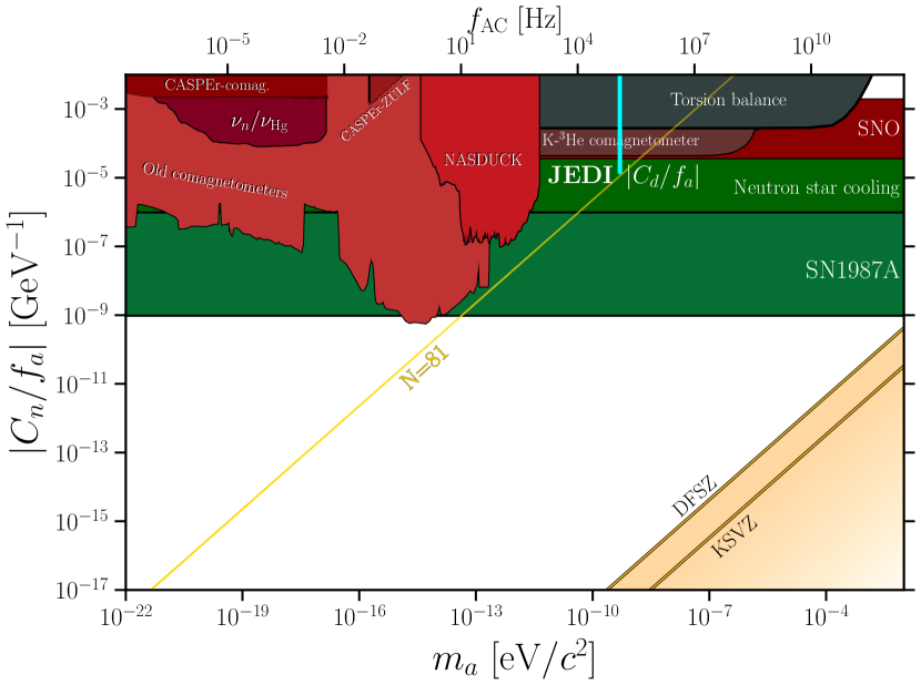
Figure 21: Figure displaying the ALP-neutron coupling $|C_{n}/f_{a}|$ from various experimental results (CASPEr-comag. [97], $\nu_{n}/\nu_{Hg}$ [25], CASPEr-Zulf [98], Old comagnetometers [95], NASDUCK [96], Torsion balance [99], K³He comagnetometer [100], SNO [101], Neutron star cooling [102], SN1987A [94]). The 90% upper bound on the ALP-deuteron coupling, $|C_{d}/f_{a}|$ from the JEDI experiment, is shown in cyan, and the corresponding $Z_{\mathcal{N}}$ axion line, labelled $\mathcal{N}=81$ and parallel to the DFSZ and KSVZ axion lines, is displayed in yellow. The limits from supernova SN1987A, as calculated in [94] (see also [93]), are presented in green. Figure courtesy [74, 12].

It should be noted that [25] has assumed $\rho_{\mathrm{LDM}}=$0.4\text{\,}\mathrm{GeV}\text{/}{\mathrm{cm}}^{3}$$ in contrast to $\rho_{\mathrm{LDM}}=$0.55\text{\,}\mathrm{GeV}\text{/}{\mathrm{cm}}^{3}$$ assumed in this paper. Thus, quoted coupling constants in this paper are $\approx 0.85$ times smaller compared to [25].

V Conclusions and Outlook

This paper presents an experiment conducted to demonstrate a new method to search for ALPs using an in-plane polarized deuteron beam in a storage ring. The polarization vector of the deuteron beam is influenced by ALPs due to two effects. First ALPs introduce an oscillating electric dipole moment (EDM) causing a spin rotation around a radial axis in the storage ring and second, the so-called axion wind or pseudomagnetic effect resulting in a spin rotation around the longitudinal axis. Storage ring experiments are specifically sensitive to the second effect because it scales with the velocity of the particles with respect to the axion field which moreover always points tangentially to the beam, i.e., in the same direction in the comoving (rest) frame of the beam particle.

The experiment did not see any ALP signal within the achieved sensitivity. An upper limit on the deuteron oscillating EDM is quoted for the first time. In the mass range $m_{a}=$ $0.4950.502\text{\,}\mathrm{neV}\text{/}{\mathrm{\text{$c$}}}^{2}$ oscillating EDM values above $\sim 10^{-22}\,$\text{\,}\mathrm{\text{$e$}}\text{\,}\mathrm{cm}\text{/}$$ are excluded by this experiment at least at a 90% level, assuming a direct EDM coupling. Constraints on other axion/ALP coupling strengths, like the ALP coupling to the EDM operator of the deuteron, $g_{ad\gamma}$, the ALP-gluon coupling of the deuteron, $C_{G}^{d}/f_{a}$ and the ALP (pseudo-magnetic) coupling to the deuteron spin $C_{d}/f_{a}$ were estimated as well.

As a proof of principle for ALP searches in storage rings, this experiment was just an exploratory study where the actual data taking period for the axion search was only four days. In future experiments with extended beam times and higher beam intensities, the sensitivity can be increased by at least an order of magnitude. Systematic effects are not expected to play an important role since one is looking for an AC effect at a particular frequency.

In the future, new type of storage rings to measure the permanent EDM of charged hadrons are planned [29]. This would allow the search for axions essentially in the whole mass range displayed in Figures 19-21. For this kind of storage rings it is proposed to use a combination of radial electric and vertical magnetic bending fields. In this case the spin precession frequency $\vec{\Omega}_{\mathrm{MDM}}-\vec{\Omega}_{\mathrm{rev}}$ is given by

$$\vec{\Omega}_{\mathrm{MDM}}-\vec{\Omega}_{\mathrm{rev}}=$$ (43)

$$-\frac{q}{m}~{}\left[G\vec{B}-\left(G-\frac{1}{\gamma^{2}-1}\right)\frac{\vec{\beta}\times\vec{E}}{c}\right]\,.$$

By using appropriate combinations of the electric and magnetic field, the amplitude of $\vec{\Omega}_{\mathrm{MDM}}-\vec{\Omega}_{\mathrm{rev}}$ can be varied from 0 to the values corresponding to $\omega_{a}=m_{a}c^{2}/\hbar\simeq 10^{-9}\,$\text{\,}\mathrm{e}\mathrm{V}\mathrm{/}\hbar$$ as described in  [103]. In that case, the relation of the EDM angular velocity (cf. Eq. (15)) becomes

$$\vec{\Omega}_{\mathrm{EDM}}=-\frac{1}{S\hbar}d(t)\left(\vec{E}+c\vec{\beta}\times\vec{B}\right)\,,$$ (44)

but still agrees with the second line of Eq. (36) when expressed as a function of the angular velocity of beam revolution. Also the relation of the axion-wind angular velocity remains unchanged, see Eq. (16) and the third line of Eq. (36).

Recently, various ideas have been discussed in the literature to extend the here presented and established storage ring searches for axions/ALPs: namely, by applying, e.g., static Wien filters or modulating radio-frequency cavities, see [44], or by using radio-frequency Wien filters operating at the sidebands of the axion frequency $\omega_{a}$ and $\Omega_{\mathrm{MDM}}$ as discussed in [30].

This kind of experiments can be further explored at facilities like RHIC, NICA or GSI/FAIR where polarized hadrons beams are either available, planned or could be added to the physics program. Using different particles (protons, deuterons, nuclei and even leptons) would allow to study the influence of spin and isospin on various couplings. Moreover, it offers the possibility to perform measurements with different $G$-factors.

Appendix A Calculation of the Relative In-Plane Polarization Directions Using Four Bunches

The signal of an ALP in a storage ring requires that the oscillation of the EDM be in phase with the rotation of the deuteron polarization in the ring plane. Specifically, the maximum value of the EDM must occur when the polarization is oriented perpendicular to the direction of the electric field in the particle frame of reference. During the search, the phase of the ALP is unknown. In order to make the effect visible for any phase, we chose to operate the COSY RF on the fourth harmonic $(h=4)$ of the revolution frequency and store four beam bunches. This appendix will demonstrate that this choice provides beams with different phases between the oscillating EDM and the direction of the rotating beam polarization. Since the wavelength of the axion field is much larger than the physical size of the COSY ring, this allows the ALP signal to be observed regardless of the ALP phase.

The beam is loaded into COSY with the polarization oriented in the vertical direction. Rotation of the polarization into the ring plane is accomplished by operating an RF solenoid for a brief period of time. If the solenoid RF operates at the same frequency as the in-plane rotation of the polarization, then the small rotation induced by the solenoid will accumulate. Continuous running of the solenoid produces an oscillation of the vertical polarization component. If the solenoid is stopped when the polarization reaches the in-plane orientation, then the beam is prepared for the experiment.

This result may be calculated using a simple series of classical rotations, each associated with one turn of the beam around COSY. For this a comoving coordinate system is used with the $z$-axis pointing in momentum direction, the $y$-axis upwards parallel to the magnetic field, and, consequently, the $x$-axis from the center of the ring outwards as the beam is rotating clockwise. In the model, the polarization is described by a vector, $[p_{x},\,p_{y},\,p_{z}]$ with the initial polarization $[0,1,0]$. One turn around the ring is described by two rotations, one ($\theta$) for the precession in the ring magnets and another ($\alpha$) for the precession in the RF solenoid, as shown in Eq. (45):

$$\!\begin{bmatrix}p^{\prime}_{x}\\ p^{\prime}_{y}\\ p^{\prime}_{z}\\ \end{bmatrix}\!=\!\begin{bmatrix}\cos\alpha&-\sin\alpha&0\\ \sin\alpha&\cos\alpha&0\\ 0&0&1\\ \end{bmatrix}\!\!\begin{bmatrix}\cos\theta&0&\sin\theta\\ 0&1&0\\ -\sin\theta&0&\cos\theta\\ \end{bmatrix}\!\!\begin{bmatrix}p_{x}\\ p_{y}\\ p_{z}\\ \end{bmatrix}.$$ (45)

The primed spin vector is the result of one revolution of the beam around the ring. The rotations may be treated separately since the length of the RF solenoid is very short compared with the circumference of the ring. For the purposes of a computer-based calculation, the precession of the spins about the $y$-axis in the ring magnets per turn is given by $\theta=-2\pi G\gamma$, where $G=-0.1429875424$ is the deuteron magnetic anomaly and $\gamma=1.1259762$ is the relativistic factor at the initial beam energy. This rotation is the same for every turn. The RF solenoid operates on a harmonic of the revolution frequency and with an adjustable strength $4\pi\epsilon_{\mathrm{sol}}$, such that $\epsilon_{\mathrm{sol}}=f_{\mathrm{sol}}/f_{\mathrm{rev}}$ with $f_{\mathrm{sol}}$ being the frequency of the resulting driven spin oscillations. Thus $\alpha=4\pi\epsilon_{\mathrm{sol}}\cos[2\pi n(1+G\gamma)+\phi]$ where $n$ is the turn count (or the number of times the two rotations have been applied) and $\phi$ is a phase that will be described later. For each turn of the beam, the operation shown in Eq. (45) is repeated based on the result of the previous series of rotations. The solenoid rotation $\alpha$ is cumulative, adding another $4\pi\epsilon_{\mathrm{sol}}\cos[2\pi n(1+G\gamma)]$ to the previous value on each turn.

A program was written to complete the numerical sum of all rotations. In the model, $2\times 10^{6}$ turns were used, and a value of $4\pi\epsilon_{\mathrm{sol}}=1.5708\times 10^{-6}$ brought the vertical polarization very close to zero.

To simulate what happens for each of the four beam bunches, we need to repeat the calculation described above, but with an initial phase added to the RF solenoid angle $\alpha$ to describe the delay in the phase for each bunch. For the first bunch, denoted as B0, $\phi=0$. For the three subsequent bunches, the starting phase is $U(1+G\gamma)$ where $U=\pi/2,\ \pi,\ \textrm{and}\ 3\pi/2$ for bunches B1, B2, and B3 respectively.

The orientation of the polarization at the end of this process can be described using the $x$ and $z$ coordinates as follows:

Table 6: Model calculation of bunch spin directions as measured at a fixed point in the ring, e.g., at the polarimeter.

Bunch	$x$	$z$	Angle [rad]	Angle B(n-1)-B(n)
B0	-0.639562	0.768740	-0.693928
B1	-0.904313	-0.426870	-2.011825	1.317897
B2	0.187022	-0.982356	-3.328722	1.317897
B3	0.997903	-0.064724	-4.647619	1.317897
B0 (again)				2.329493

The angle starts at the $z$ axis. The first four columns of Table 6 show the results at the end of $2\times 10^{6}$ turns. The last column shows the differences in the polarization directions between adjacent bunches, as predicted by the rotation model. The phase angles in the next to last column apply at the time that the bunch lands in the ring plane, which is different for each bunch. There is also a polarimeter in the COSY ring that is capable of measuring the phase at the beginning of each 4-second time interval. It is worth noting that the spacing between the bunches is not equal across the break from B3 to B0. Thus, we should be able to tell from the relative phases which bunch is the first. Sample results are given in Fig. 22.

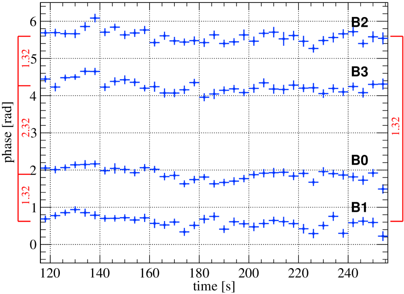
Figure 22: Measurements of the phase of the in-plane polarization of a four-bunch beam as a function of the time in the store after the RF solenoid is turned off. The four bunches are B0, B1, B2, and B3. The differences in phase angle are indicated by the red diagram that includes the relative bunch angles in radians. A fixed value of the spin tune $G\gamma$ is assumed during the analysis in order to freeze any phase drift with time.

The match of the phase differences in Fig. 22 with the predictions in Table 6 (column 5) shows that the process of using an RF solenoid to rotate the spins into the horizontal plane matches the model.

Using the model results as a starting point, we can extrapolate forward in the calculation to the same point in time for each bunch. If we choose the moment when the rotation of B3 to the horizontal plane is complete, then the in-plane rotation of bunches B0, B1, and B2 move forward by $3\pi/2$, $\pi$, and $\pi/2$, respectively. This produces a final orientation of the polarization given by Table 7.

Table 7: Model calculation of bunch spin directions as measured at a fixed point in time, i.e, when the bunch B3 is completely rotated into the horizontal plane.

Bunch	$x$	$z$
B0	0.064724	0.997903
B1	-0.997903	0.064724
B2	-0.064724	-0.997903
B3 (no change)	0.997903	-0.064724

An inspection of the $x$ and $z$ columns shows that these four polarization directions form right angles to each other in the beam coordinate system, thus mapping out a space in all directions. The rotation of the ALP EDM is generated by the presence of an electric field in the rest frame of the deuterons as they pass through the ring magnets and are subject to a vertical lab magnetic field. This induces a force on the deuterons, $\vec{F}=e\,c\vec{\beta}\times\vec{B}$, that bends them into the closed orbit around the ring. The resulting electric field in the comoving frame also creates a torque on the oscillating EDM to the extent that the latter is perpendicular to the field at the time that the EDM is at an extreme point in its oscillation. Note that the electric field points toward the center of the ring. With this assortment of polarization directions, all phases (represented by sine and cosine functions) will generate a measurable change in the vertical polarization and no ALP field will go undetected due to phase mismatch. In addition, the presence of polarizations of opposite sign ensures that any non-zero offset in the polarimeter that measures the size of the resonant jump will be offset by a jump on the opposite bunch that is of equal and opposite sign.

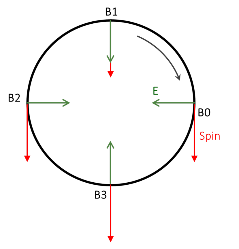
Figure 23: Diagram showing the orientations of the polarization relative to the electric field for the four bunches circulating in the storage ring, as given in Table 7. The black arrow shows the direction of the clockwise rotating beam while the rotation of the spins of the deuterons in the comoving frame and the order of the bunches on the ring (B$i$, $i=0,1,2,3$) are counterclockwise (all viewed from above).

The orientations of the polarization relative to the electric field are illustrated by the diagram in Fig. 23. It then becomes clear that the polarization directions for each of the bunches relative to the local electric field is perpendicular to the bunch preceeding it. All the polarizations are either parallel to or perpendicular to their respective electric fields. This figure assumes a circular ring without straight sections and a clockwise rotating beam viewed from above.

These calculations may be repeated for the case of the $1-G\gamma$ harmonic. Here, the resulting phase gaps have a different pattern, which was also confirmed experimentally using the phase measurements. The modeling shows that a good polarization distribution among the four bunches is possible using either harmonic for the RF solenoid. There is a sort of symmetry between the two possibilities. The sets of phases as measured by a fixed polarimeter looking at the bunches one at a time are distinctive and allow one to pick out the “first” bunch in each group from its location next to the single gap that is different from all the rest. This result is impervious to a number of potential issues, including whether or not the RF solenoid switching time is gradual (as is the case experimentally) or instantaneous (as it is in the model).

Appendix B Calculation of the Sensitivity Calibration

Previous calculations of the response of the COSY storage ring have been made using a “no-lattice” model [60, 61] of successive rotations without a breakdown for each element of the ring. While the rotations in the bending magnets are continuous in this model, other devices such as the RF solenoid (see Appendix A) and the Wien filter are relatively short and may be treated as having zero length. The spin rotation per turn due to the bending magnet is about the vertical axis and given by the rotation vector $\vec{\theta}=-2\pi G\gamma\vec{e}_{y}$ $(=\theta\vec{e}_{y})$. When we include the EDM, this introduces another continuous effect with a rotation about the radial (pointing outward from the center of the bend assuming $d>0$ in Eq. (15)) axis given by $\vec{\psi}=2\pi\vec{\Omega}_{\mathrm{EDM}}/|\vec{\Omega}_{\mathrm{rev}}|$ $(=\psi\vec{e}_{x})$. As a result, one gets a new, combined rotation about a new axis $\vec{\chi}$:

$$\vec{\chi}=\vec{\theta}+\vec{\psi}.$$ (46)

The situation is depicted in Fig. 24.

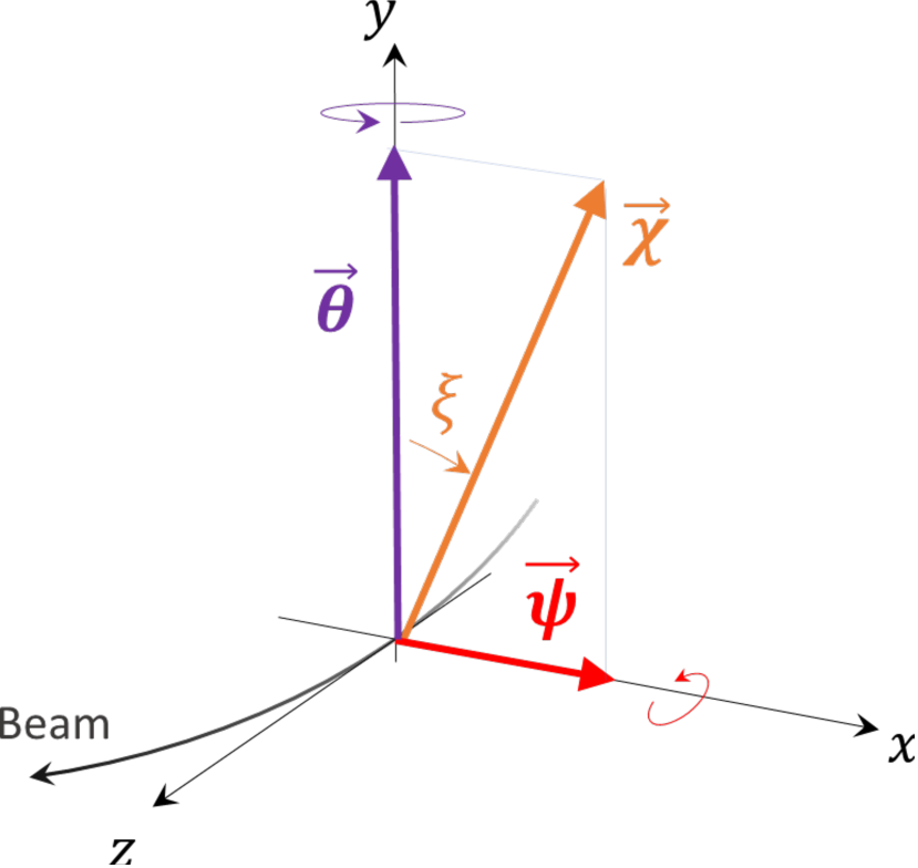
Figure 24: Diagram showing the orientation of the rotation vectors associated with an EDM precession in the presence of bending in a storage ring. Coordinates and the bent particle path are shown. The total rotation $\vec{\chi}$ is the vector sum of $\vec{\theta}$ and $\vec{\psi}$. The angle between $\vec{\theta}$ and $\vec{\chi}$, denoted by $\xi$, is the angle of the coordinate system rotation (see text). The size of $\vec{\psi}$ in this figure is exaggerated to make it visible to the reader.

To calculate the result within the no-lattice model, we chose to tilt the reference frame about the $z$-axis so that the new $y$-axis lies along the total rotation vector $\vec{\chi}$. The angle of tilt becomes

$$\xi=\arctan\frac{\psi}{\theta}$$ (47)

One turn through the storage ring is represented by

$$\!\begin{bmatrix}p^{\prime}_{x}\\ p^{\prime}_{y}\\ p^{\prime}_{z}\\ \end{bmatrix}=\begin{bmatrix}\cos\xi&-\sin\xi&0\\ \sin\xi&\cos\xi&0\\ 0&0&1\\ \end{bmatrix}\begin{bmatrix}\cos\chi&0&\sin\chi\\ 0&1&0\\ -\sin\chi&0&\cos\chi\\ \end{bmatrix}$$ (48)

$$\times\begin{bmatrix}\cos\xi&\sin\xi&0\\ -\sin\xi&\cos\xi&0\\ 0&0&1\\ \end{bmatrix}\begin{bmatrix}p_{x}\\ p_{y}\\ p_{z}\\ \end{bmatrix}\\$$ (49)

where the vector $[p_{x},p_{y},p_{z}]$ represents the initial projection of the polarization along the axes shown in Fig. 24, and $[p^{\prime}_{x},p^{\prime}_{y},p^{\prime}_{z}]$ represents the resulting polarization. The first and third square matrices handle the transformation of the coordinate system while the main rotation is described by the middle matrix.

In the simulation used to calibrate the response of the system to an axion, the revolution frequency of the deuteron was ramped. The ramp was centered at the nominal beam frequency of $f_{\mathrm{rev}}=$$750\,602.6\text{\,}\mathrm{Hz}\text{/}$, with a $100\text{\,}\mathrm{H}\mathrm{z}$ scanning range. The ramp rate for $f_{\mathrm{rev}}$ in the calculation was $1\text{\,}\mathrm{Hz}\text{/}\mathrm{s}$. As the ramp was followed, the small changes to the relativistic factor $\gamma$ and the elapsed time of a single turn 1/$f_{\mathrm{rev}}$, were followed as discussed in the main text.

In Eq. (7) the oscillating part of the EDM is described by

$$d_{\mathrm{osc}}(t)=d_{\mathrm{AC}}\cos\big{(}\omega_{a}(t-t_{0})+\phi_{a}(t_{0})\big{)}.$$ (50)

This can be expressed in terms of the EDM rotation angle $\psi_{\mathrm{osc}}(t)$ as

$$\psi_{\mathrm{osc}}(t)=\psi_{\mathrm{AC}}\cos\big{(}\omega_{a}(t-t_{0})+\phi_{a}(t_{0})\big{)}.$$ (51)

In this equation, $t_{0}$ was assumed to be the time at the start of the scan. Thus, time accumulated with an ever-decreasing time step for each turn as the scan slowly ramped up the revolution frequency. This caused the EDM oscillation, initially out of step with the polarization rotation, to fall in step and then out of step as the scan proceeded. Depending on the exact conditions at the beginning, the individual accumulation of the vertical polarization $y^{\prime}$ as the resonance is crossed may be any value between its positive and negative limits. Thus, the size of the calculated jump will vary similarly. In order to know the maximum jump possible, the calculation must be run with two orthogonal phases such as $\phi_{a}=0$ and $\pi/2$. Then the sizes of the jumps are added in quadrature to obtain the final value of the jump size.

The numerical simulation used in the calibration of the sensitivity began with a particular size of the oscillating EDM and scanning rate to calculate the expected polarization jump. For jumps that are much less than one (assuming complete polarization), the relationship between the EDM size and the jump is nearly linear. This allows us to use just the slope given by the calibration. One example of such a calculation begins with an EDM rotation of $\psi_{\mathrm{AC}}=$8\text{\times}{10}^{-9}$$ rad/turn and a scanning rate of 1 Hz/s. After calculating the jump for two orthogonal choices of the axion phase, the results were combined and gave a jump of $\Delta p_{y}=0.0066$, which is normalized to a beam polarization of one. Tests with the calibration program demonstrate that the jump scales with the reciprocal of the square root of the ramping rate in the linear region. The ratio of EDM rotation to total polarization jump must be scaled by $w=\sqrt{\text{ramp(actual)}/\text{ramp(calib.)}}=0.775$ for the faster scans and 0.700 for the slower scans.

The value of ramp(calib.) is 1.00 and the values of ramp(actual) are found in column 3 of Table 3 where the rates are 0.600 Hz/s for the fast scans and 0.490 Hz/s for the slow scans. The ratio or slope between $\psi_{\mathrm{AC}}$ and $\Delta p_{y}$ then becomes $9.35\text{\times}{10}^{-7}$ rad/turn for the fast scans and $8.48\text{\times}{10}^{-7}$ rad/turn for the slow scans.

Using the first (radially pointing) term of Eq. (36) we can describe the amplitude of the contribution to the determination of the oscillating EDM in terms of $\psi_{\mathrm{AC}}=2\pi\Omega_{a}/|\vec{\Omega}_{\mathrm{rev}}|$ where $\Omega_{a}$ is the amplitude of the oscillating angular velocity $\vec{\Omega}_{a(t)}$, by

$$d_{\mathrm{AC}}=\frac{1}{2\pi}\frac{S\hbar q}{\beta\gamma m_{d}c}\,\frac{w}{0.958}\,\psi_{\mathrm{AC}}\,,$$ (52)

where the spin $S$ is equal to one. The factor $w$ corrects for the ramp rate and 0.958 corrects for the alternating straight and curves sections in the COSY ring (see end of Section II.1). For ease of connecting with the parameters of the COSY ring, the charge $q$ and the denominator of the first fraction may be swapped for the beam momentum expressed as $(B\rho)$. Then, in the usual EDM units of $\text{\,}\mathrm{\text{$e$}}\text{\,}\mathrm{cm}\text{/}$ and expressed in terms of the above quoted slope between $\psi_{\mathrm{AC}}$ and the jump $\Delta p_{y}$ we have

$$|d_{\mathrm{AC}}|=\frac{1}{2\pi}\frac{\hbar}{B\rho}\,\frac{w}{0.958}\,\left|\frac{\psi_{\mathrm{AC}}}{\Delta p_{y}}\right|_{\mathrm{calib.}}A\,,$$ (53)

where $A$ is the true value of the upper limit on the magnitude of the jump. The second fraction in this expression has the value of $\hbar/B\rho=$3.26\text{\times}{10}^{-35}$$ J$\cdot$s$\cdot($T$\cdot$m$)^{-1}=$2.03\text{\times}{10}^{-14}\text{\,}\mathrm{\text{$e$}}\text{\,}\mathrm{cm}\text{/}$$ while the rest of the expression is dimensionless. In this way, Eq. (35) was derived – including the values $316$ and $286$, respectively, of the coefficient $\lambda$. For typical values of the true $A$, values for $d_{\mathrm{AC}}$ usually lie below $10^{-22}\,$\text{\,}\mathrm{\text{$e$}}\text{\,}\mathrm{cm}\text{/}$$.

The oscillating EDM has a period that is comparable in size to the revolution frequency. We made the approximation that the size of the EDM could be represented at any moment by its average value during a time interval that was chosen to be a fraction of a turn as the beam circulated in the storage ring. The 3-matrix formula shown above in Eq. (48) was repeated $N$ times during each turn. For the calculations reported here, we chose $N=15$ for which the calculations had converged to a precision of $0.1\%$.

The calculations were repeated for spin rotation with respect to the longitudinal axis of the beam arising from axion-wind effect and the calibration matched the rotation along radial axis as explained in this appendix.

References

- [1] R. D. Peccei and H. R. Quinn. “CP Conservation in the Presence of Instantons”. Phys. Rev. Lett., 38, 1440 (1977). doi:10.1103/PhysRevLett.38.1440.
- [2] R. D. Peccei and H. R. Quinn. “Constraints Imposed by CP Conservation in the Presence of Instantons”. Phys. Rev. D, 16, 1791 (1977). doi:10.1103/PhysRevD.16.1791.
- [3] S. Weinberg. “A New Light Boson?” Phys. Rev. Lett., 40, 223 (1978). doi:10.1103/PhysRevLett.40.223.
- [4] F. Wilczek. “Problem of Strong and Invariance in the Presence of Instantons”. Phys. Rev. Lett., 40, 279 (1978). doi:10.1103/PhysRevLett.40.279.
- [5] R. D. Peccei. “The Strong CP problem and axions”. Lect. Notes Phys., 741, 3 (2008). doi:10.1007/978-3-540-73518-2_1. eprint hep-ph/0607268.
- [6] Y. Asano et al. “Search for a Rare Decay Mode K+ — pi+ Neutrino anti-neutrino and Axion”. Phys. Lett. B, 107, 159 (1981). doi:10.1016/0370-2693(81)91172-2.
- [7] J. E. Kim. “Weak Interaction Singlet and Strong CP Invariance”. Phys. Rev. Lett., 43, 103 (1979). doi:10.1103/PhysRevLett.43.103.
- [8] M. A. Shifman, A. I. Vainshtein, and V. I. Zakharov. “Can Confinement Ensure Natural CP Invariance of Strong Interactions?” Nucl. Phys. B, 166, 493 (1980). doi:10.1016/0550-3213(80)90209-6.
- [9] M. Dine, W. Fischler, and M. Srednicki. “A Simple Solution to the Strong CP Problem with a Harmless Axion”. Phys. Lett. B, 104, 199 (1981). doi:10.1016/0370-2693(81)90590-6.
- [10] A. R. Zhitnitsky. “On Possible Suppression of the Axion Hadron Interactions. (In Russian)”. Sov. J. Nucl. Phys., 31, 260 (1980).
- [11] M. Gorghetto and G. Villadoro. “Topological Susceptibility and QCD Axion Mass: QED and NNLO corrections”. JHEP, 2019(03), 033 (2019). doi:10.1007/JHEP03(2019)033. eprint 1812.01008.
- [12] R. L. Workman and Others. “Review of Particle Physics”. PTEP, 2022, 083C01 (2022). doi:10.1093/ptep/ptac097.
- [13] A. Hook. “Solving the Hierarchy Problem Discretely”. Phys. Rev. Lett., 120(26), 261802 (2018). doi:10.1103/PhysRevLett.120.261802. eprint 1802.10093.
- [14] L. Di Luzio et al. “An even lighter QCD axion”. JHEP, 2021(05), 184 (2021). doi:10.1007/JHEP05(2021)184. eprint 2102.00012.
- [15] L. Di Luzio et al. “Dark matter from an even lighter QCD axion: trapped misalignment”. JCAP, 2021(10), 001 (2021). doi:10.1088/1475-7516/2021/10/001. eprint 2102.01082.
- [16] P. Sikivie. “Invisible Axion Search Methods”. Rev. Mod. Phys., 93(1), 015004 (2021). doi:10.1103/RevModPhys.93.015004. eprint 2003.02206.
- [17] P. W. Graham and S. Rajendran. “Axion dark matter detection with cold molecules”. Phys. Rev. D, 84, 055013 (2011). doi:10.1103/PhysRevD.84.055013.
- [18] P. W. Graham and S. Rajendran. “New observables for direct detection of axion dark matter”. Phys. Rev. D, 88, 035023 (2013). doi:10.1103/PhysRevD.88.035023.
- [19] Y. V. Stadnik and V. V. Flambaum. “Axion-induced effects in atoms, molecules, and nuclei: Parity nonconservation, anapole moments, electric dipole moments, and spin-gravity and spin-axion momentum couplings”. Phys. Rev. D, 89(4), 043522 (2014). doi:10.1103/PhysRevD.89.043522. eprint 1312.6667.
- [20] D. Budker et al. “Proposal for a Cosmic Axion Spin Precession Experiment (CASPEr)”. Phys. Rev. X, 4(2), 021030 (2014). doi:10.1103/PhysRevX.4.021030. eprint 1306.6089.
- [21] P. Sikivie. “Experimental Tests of the Invisible Axion”. Phys. Rev. Lett., 51, 1415 (1983). doi:10.1103/PhysRevLett.51.1415. [Erratum: Phys.Rev.Lett. 52, 695 (1984)].
- [22] P. Sikivie. “Detection Rates for ’Invisible’ Axion Searches”. Phys. Rev. D, 32, 2988 (1985). doi:10.1103/PhysRevD.36.974. [Erratum: Phys.Rev.D 36, 974 (1987)].
- [23] P. W. Graham et al. “Experimental Searches for the Axion and Axion-Like Particles”. Ann. Rev. Nucl. Part. Sci., 65, 485 (2015). doi:10.1146/annurev-nucl-102014-022120. eprint 1602.00039.
- [24] W. Bernreuther. “The Electric dipole moment of the muon”. Z. Phys. C, 56, S97 (1992). doi:10.1007/BF02426781.
- [25] C. Abel et al. “Search for axionlike dark matter through nuclear spin precession in electric and magnetic fields”. Physical Review X, 7, 041034 (2017). ISSN 2160-3308. doi:10.1103/PhysRevX.7.041034.
- [26] T. S. Roussy et al. “Experimental Constraint on Axionlike Particles over Seven Orders of Magnitude in Mass”. Phys. Rev. Lett., 126, 171301 (2021). doi:10.1103/PhysRevLett.126.171301. eprint 2006.15787.
- [27] S. P. Chang et al. “Axion dark matter search using the storage ring EDM method”. PoS, PSTP2017, 036 (2018). doi:10.22323/1.324.0036.
- [28] S. P. Chang et al. “Axionlike dark matter search using the storage ring EDM method”. Phys. Rev. D, 99, 083002 (2019). doi:10.1103/PhysRevD.99.083002.
- [29] F. Abusaif et al. Storage ring to search for electric dipole moments of charged particles : feasibility study. CERN Yellow Reports. Monographs, ISSN 2519-8068, eISSN 2519-8076; 3. CERN, Geneva (2021). ISBN 978-92-9083-607-0. doi:10.23731/CYRM-2021-003.
- [30] O. Kim and Y. K. Semertzidis. “New method of probing an oscillating EDM induced by axionlike dark matter using an RF Wien filter in storage rings”. Phys. Rev. D, 104(9), 096006 (2021). doi:10.1103/PhysRevD.104.096006. eprint 2105.06655.
- [31] L. Krauss et al. “Calculations for Cosmic Axion Detection”. Phys. Rev. Lett., 55, 1797 (1985). doi:10.1103/PhysRevLett.55.1797.
- [32] H. Georgi, D. B. Kaplan, and L. Randall. “Manifesting the Invisible Axion at Low-energies”. Phys. Lett. B, 169, 73 (1986). doi:10.1016/0370-2693(86)90688-X.
- [33] G. Raffelt and D. Seckel. “Bounds on Exotic Particle Interactions from SN 1987a”. Phys. Rev. Lett., 60, 1793 (1988). doi:10.1103/PhysRevLett.60.1793.
- [34] K. Choi, K. Kang, and J. E. Kim. “Invisible Axion Emissions From SN1987A”. Phys. Rev. Lett., 62, 849 (1989). doi:10.1103/PhysRevLett.62.849.
- [35] M. Carena and R. D. Peccei. “The Effective Lagrangian for Axion Emission From SN1987A”. Phys. Rev. D, 40, 652 (1989). doi:10.1103/PhysRevD.40.652.
- [36] R. Barbieri et al. “Axion to magnon conversion: a scheme for the detection of galactic axions”. Phys. Lett. B, 226, 357 (1989). doi:10.1016/0370-2693(89)91209-4.
- [37] P. V. Vorob’ev, I. V. Kolokolov, and V. F. Fogel. “Ferromagnetic detector of (pseudo)Goldstone bosons”. JETP Lett., 50, 65 (1989). http://jetpletters.ru/ps/1125/article_17041.shtml.
- [38] A. I. Kakhidze and I. V. Kolokolov. “Antiferromagnetic axions detector”. Sov. Phys. JETP, 72, 598 (1991).
- [39] P. V. Vorob’ev, A. I. Kakhidze, and I. V. Kolokolov. “Axion wind: A Search for cosmological axion condensate”. Phys. Atom. Nucl., 58, 959 (1995).
- [40] P. W. Graham et al. “Spin Precession Experiments for Light Axionic Dark Matter”. Phys. Rev. D, 97(5), 055006 (2018). doi:10.1103/PhysRevD.97.055006. eprint 1709.07852.
- [41] Y. Stadnik. Manifestations of Dark Matter and Variations of the Fundamental Constants of Nature in Atoms and Astrophysical Phenomena. Ph.D. thesis, New South Wales U. (2017). doi:10.1007/978-3-319-63417-3.
- [42] C. Smorra et al. “Direct limits on the interaction of antiprotons with axion-like dark matter”. Nature, 575(7782), 310 (2019). doi:10.1038/s41586-019-1727-9. eprint 2006.00255.
- [43] P. W. Graham et al. “Storage ring probes of dark matter and dark energy”. Phys. Rev. D, 103(5), 055010 (2021). doi:10.1103/PhysRevD.103.055010. eprint 2005.11867.
- [44] A. J. Silenko. “Relativistic spin dynamics conditioned by dark matter axions”. Eur. Phys. J. C, 82(10), 856 (2022). doi:10.1140/epjc/s10052-022-10827-7. eprint 2109.05576.
- [45] N. N. Nikolaev. “Spin of protons in NICA and PTR storage rings as an axion antenna”. Pisma Zh. Eksp. Teor. Fiz., 115(11), 683 (2022). doi:10.1134/S0021364022600653.
- [46] A. J. Silenko. “High precision description and new properties of a spin-1 particle in a magnetic field”. Phys. Rev. D, 89(12), 121701 (2014). doi:10.1103/PhysRevD.89.121701. eprint 1404.4953.
- [47] A. J. Silenko. “General description of spin motion in storage rings in the presence of oscillating horizontal fields”. EPL, 118(6), 61003 (2017). doi:10.1209/0295-5075/118/61003. eprint 1706.02065.
- [48] V. Bargmann, L. Michel, and V. L. Telegdi. “Precession of the polarization of particles moving in a homogeneous electromagnetic field”. Phys. Rev. Lett., 2, 435 (1959). doi:10.1103/PhysRevLett.2.435.
- [49] T. Fukuyama and A. J. Silenko. “Derivation of Generalized Thomas-Bargmann-Michel-Telegdi Equation for a Particle with Electric Dipole Moment”. Int. J. Mod. Phys., A28, 1350147 (2013). doi:10.1142/S0217751X13501479. eprint 1308.1580.
- [50] E. Stephenson. “A Search for Axion-like Particles with a Horizontally Polarized Beam In a Storage Ring”. PoS, PSTP2019, 018 (2020). doi:10.22323/1.379.0018.
- [51] G. Guidoboni et al. “How to reach a thousand-second in-plane polarization lifetime with deuterons in a storage ring”. Phys. Rev. Lett., 117, 054801 (2016). doi:10.1103/PhysRevLett.117.054801.
- [52] D. Eversmann et al. “New method for a continuous determination of the spin tune in storage rings and implications for precision experiments”. Phys. Rev. Lett., 115, 094801 (2015). doi:10.1103/PhysRevLett.115.094801.
- [53] R. Maier. “Cooler synchrotron COSY: Performance and perspectives”. Nucl. Instrum. Meth. A, 390, 1 (1997). doi:10.1016/S0168-9002(97)00324-0.
- [54] W. Haeberli. “Sources of polarized ions”. Annual Review of Nuclear Science, 17(1), 373 (1967). doi:10.1146/annurev.ns.17.120167.002105.
- [55] D. Chiladze et al. “Determination of deuteron beam polarizations at COSY”. Phys. Rev. ST Accel. Beams, 9, 050101 (2006). doi:10.1103/PhysRevSTAB.9.050101.
- [56] M. Tanifuji. Polarization Phenomena in Physics: Applications to Nuclear Reactions. World Scientific, Singapore (2018). ISBN 987-981-3230-88-0. doi:10.1142/10731.
- [57] H. H. Barschall and W. Haeberli (eds.). The Madison Convention, Polarization Phenomena in Nuclear Reactions. University of Wisconsin Press, Madison, WI (1971). https://www.osti.gov/biblio/4726823.
- [58] F. Müller et al. “Measurement of deuteron carbon vector analyzing powers in the kinetic energy range 170–380 MeV”. Eur. Phys. J. A, 56, 1 (2020). ISSN 1434-601X. doi:10.1140/EPJA/S10050-020-00215-8.
- [59] Z. Bagdasarian et al. “Measuring the polarization of a rapidly precessing deuteron beam”. Phys. Rev. Accel. Beams, 17, 052803 (2014). doi:10.1103/PhysRevSTAB.17.052803.
- [60] P. Benati et al. “Synchrotron oscillation effects on an rf-solenoid spin resonance”. Phys. Rev. Accel. Beams, 15, 124202 (2012). doi:10.1103/PhysRevSTAB.15.124202.
- [61] P. Benati et al. “Erratum: Synchrotron oscillation effects on an rf-solenoid spin resonance [Phys. Rev. ST Accel. Beams 15, 124202 (2012)]”. Phys. Rev. Accel. Beams, 16, 049901 (2013). doi:10.1103/PhysRevSTAB.16.049901.
- [62] G. Guidoboni et al. “Connection between zero chromaticity and long in-plane polarization lifetime in a magnetic storage ring”. Phys. Rev. Accel. Beams, 21, 024201 (2018). doi:10.1103/PhysRevAccelBeams.21.024201.
- [63] J. Slim et al. “Electromagnetic Simulation and Design of a Novel Waveguide RF Wien Filter for Electric Dipole Moment Measurements of Protons and Deuterons”. Nuclear Instruments and Methods in Physics Research Section A: Accelerators, Spectrometers, Detectors and Associated Equipment, 828, 116 (2016). doi:10.1016/j.nima.2016.05.012.
- [64] J. Slim et al. “The driving circuit of the waveguide RF Wien filter for the deuteron EDM precursor experiment at COSY”. Journal of Instrumentation, 15(03), P03021 (2020). doi:10.1088/1748-0221/15/03/p03021.
- [65] F. Rathmann, N. N. Nikolaev, and J. Slim. “Spin dynamics investigations for the electric dipole moment experiment”. Phys. Rev. Accel. Beams, 23, 024601 (2020). doi:10.1103/PhysRevAccelBeams.23.024601.
- [66] J. Slim et al. “First detection of collective oscillations of a stored deuteron beam with an amplitude close to the quantum limit”. Phys. Rev. Accel. Beams, 24(12), 124601 (2021). doi:10.1103/PhysRevAccelBeams.24.124601. eprint 2101.07582.
- [67] JEDI Collaboration. “Replication Data for: First Search for Axion-Like Particles in a Storage Ring Using a Polarized Deuteron Beam” (2022). doi:10.26165/JUELICH-DATA/HHNVQ3.
- [68] G. J. Feldman and R. D. Cousins. “Unified approach to the classical statistical analysis of small signals”. Phys. Rev. D, 57, 3873 (1998). doi:10.1103/PhysRevD.57.3873.
- [69] S. P. Chang. Studies on Axion-EDM experiment using the storage ring method. Ph.D. dissertation, https://library.kaist.ac.kr/search/ctlgSearch/posesn/view.do?bibctrlno=996474&se=t0&ty=B&_csrf=cdfcdff0-c27d-4b60-9bef-cbb0967f7d6d, The Korea Advanced Institute of Science and Technology (KAIST), Daedeok Innopolis, Daejeon, South Korea (2022).
- [70] S. Plaszczynski et al. “A novel estimator of the polarization amplitude from normally distributed Stokes parameters”. Monthly Notices of the Royal Astronomical Society, 439(4), 4048 (2014). ISSN 0035-8711. doi:10.1093/mnras/stu270.
- [71] D. Eversmann, J. Pretz, and M. Rosenthal. “Amplitude estimation of a sine function based on confidence intervals and Bayes' theorem”. Journal of Instrumentation, 2016(11), P05003 (2016). doi:10.1088/1748-0221/11/05/p05003.
- [72] D. Aybas et al. “Search for axionlike dark matter using solid-state nuclear magnetic resonance”. Phys. Rev. Lett., 126, 141802 (2021). doi:10.1103/PhysRevLett.126.141802.
- [73] I. Schulthess et al. “New Limit on Axionlike Dark Matter Using Cold Neutrons”. Phys. Rev. Lett., 129(19), 191801 (2022). doi:10.1103/PhysRevLett.129.191801. eprint 2204.01454.
- [74] C. O’Hare. “cajohare/axionlimits: Axionlimits”. https://cajohare.github.io/AxionLimits/ (2020). doi:10.5281/zenodo.3932430.
- [75] N. Bar, K. Blum, and G. D’Amico. “Is there a supernova bound on axions?” Phys. Rev. D, 101(12), 123025 (2020). doi:10.1103/PhysRevD.101.123025. eprint 1907.05020.
- [76] L. Caloni et al. “Novel cosmological bounds on thermally-produced axion-like particles”. Journal of Cosmology and Astroparticle Physics, 2022(09), 021 (2022). doi:10.1088/1475-7516/2022/09/021.
- [77] M. Pospelov and A. Ritz. “Theta induced electric dipole moment of the neutron via QCD sum rules”. Phys. Rev. Lett., 83, 2526 (1999). doi:10.1103/PhysRevLett.83.2526. eprint hep-ph/9904483.
- [78] R. J. Crewther et al. “Chiral Estimate of the Electric Dipole Moment of the Neutron in Quantum Chromodynamics”. Phys. Lett. B, 88, 123 (1979). doi:10.1016/0370-2693(79)90128-X. [Erratum: Phys.Lett.B 91, 487 (1980)].
- [79] V. Baluni. “CP-nonconserving effects in quantum chromodynamics”. Phys. Rev. D, 19, 2227 (1979). doi:10.1103/PhysRevD.19.2227.
- [80] K. Ottnad et al. “New insights into the neutron electric dipole moment”. Phys. Lett. B, 687, 42 (2010). doi:10.1016/j.physletb.2010.03.005. eprint 0911.3981.
- [81] N. Yamanaka and E. Hiyama. “Enhancement of the CP-odd effect in the nuclear electric dipole moment of 6Li”. Phys. Rev. C, 91(5), 054005 (2015). doi:10.1103/PhysRevC.91.054005. eprint 1503.04446.
- [82] J. Bsaisou et al. “Nuclear Electric Dipole Moments in Chiral Effective Field Theory”. JHEP, 2015(03), 104 (2015). doi:10.1007/JHEP03(2015)104. [Erratum: JHEP 05, 083 (2015).], eprint 1411.5804.
- [83] I. B. Khriplovich and R. A. Korkin. “P and T odd electromagnetic moments of deuteron in chiral limit”. Nucl. Phys. A, 665, 365 (2000). doi:10.1016/S0375-9474(99)00403-0. eprint nucl-th/9904081.
- [84] O. Lebedev et al. “Probing CP violation with the deuteron electric dipole moment”. Phys. Rev. D, 70, 016003 (2004). doi:10.1103/PhysRevD.70.016003. eprint hep-ph/0402023.
- [85] C. P. Liu and R. G. E. Timmermans. “P- and T-odd two-nucleon interaction and the deuteron electric dipole moment”. Phys. Rev. C, 70, 055501 (2004). doi:10.1103/PhysRevC.70.055501. eprint nucl-th/0408060.
- [86] I. R. Afnan and B. F. Gibson. “Model Dependence of the 2H Electric Dipole Moment”. Phys. Rev. C, 82, 064002 (2010). doi:10.1103/PhysRevC.82.064002. eprint 1011.4968.
- [87] J. de Vries et al. “Parity- and Time-Reversal-Violating Form Factors of the Deuteron”. Phys. Rev. Lett., 107, 091804 (2011). doi:10.1103/PhysRevLett.107.091804. eprint 1102.4068.
- [88] J. Bsaisou et al. “The electric dipole moment of the deuteron from the QCD -term”. Eur. Phys. J. A, 49, 31 (2013). doi:10.1140/epja/i2013-13031-x. eprint 1209.6306.
- [89] J. Bsaisou et al. “P- and T-Violating Lagrangians in Chiral Effective Field Theory and Nuclear Electric Dipole Moments”. Annals Phys., 359, 317 (2015). doi:10.1016/j.aop.2015.04.031. eprint 1412.5471.
- [90] A. Wirzba, J. Bsaisou, and A. Nogga. “Permanent Electric Dipole Moments of Single-, Two-, and Three-Nucleon Systems”. Int. J. Mod. Phys. E, 26(01n02), 1740031 (2017). doi:10.1142/S0218301317400316. eprint 1610.00794.
- [91] A. Hook and J. Huang. “Probing axions with neutron star inspirals and other stellar processes”. JHEP, 2018(06), 036 (2018). doi:10.1007/JHEP06(2018)036. eprint 1708.08464.
- [92] K. Blum et al. “Constraining Axion Dark Matter with Big Bang Nucleosynthesis”. Phys. Lett. B, 737, 30 (2014). doi:10.1016/j.physletb.2014.07.059. eprint 1401.6460.
- [93] G. G. Raffelt. “Astrophysical axion bounds”. Lect. Notes Phys., 741, 51 (2008). doi:10.1007/978-3-540-73518-2_3. eprint hep-ph/0611350.
- [94] P. Carenza et al. “Improved axion emissivity from a supernova via nucleon-nucleon bremsstrahlung”. JCAP, 2019(10), 016 (2019). doi:10.1088/1475-7516/2019/10/016. [Erratum: JCAP 05, E01 (2020)], eprint 1906.11844.
- [95] I. M. Bloch et al. “Axion-like Relics: New Constraints from Old Comagnetometer Data”. JHEP, 2020(01), 167 (2020). doi:10.1007/JHEP01(2020)167. eprint 1907.03767.
- [96] I. M. Bloch et al. “New constraints on axion-like dark matter using a Floquet quantum detector”. Sci. Adv., 8(5), abl8919 (2022). doi:10.1126/sciadv.abl8919. eprint 2105.04603.
- [97] D. F. Jackson Kimball et al. “Overview of the Cosmic Axion Spin Precession Experiment (CASPEr)”. Springer Proc. Phys., 245, 105 (2020). doi:10.1007/978-3-030-43761-9_13. eprint 1711.08999.
- [98] A. Garcon et al. “Constraints on bosonic dark matter from ultralow-field nuclear magnetic resonance”. Sci. Adv., 5(10), eaax4539 (2019). doi:10.1126/sciadv.aax4539. eprint 1902.04644.
- [99] E. G. Adelberger et al. “Particle Physics Implications of a Recent Test of the Gravitational Inverse Sqaure Law”. Phys. Rev. Lett., 98, 131104 (2007). doi:10.1103/PhysRevLett.98.131104. eprint hep-ph/0611223.
- [100] G. Vasilakis et al. “Limits on New Long Range Nuclear Spin-Dependent Forces Set with a K-He3 Comagnetometer”. Phys. Rev. Lett., 103(26), 261801 (2009). doi:10.1103/PhysRevLett.103.261801. eprint 0809.4700.
- [101] A. Bhusal, N. Houston, and T. Li. “Searching for Solar Axions Using Data from the Sudbury Neutrino Observatory”. Phys. Rev. Lett., 126(9), 091601 (2021). doi:10.1103/PhysRevLett.126.091601. eprint 2004.02733.
- [102] M. Buschmann et al. “Upper Limit on the QCD Axion Mass from Isolated Neutron Star Cooling”. Phys. Rev. Lett., 128(9), 091102 (2022). doi:10.1103/PhysRevLett.128.091102. eprint 2111.09892.
- [103] J. Pretz et al. “Statistical sensitivity estimates for oscillating electric dipole moment measurements in storage rings”. Eur. Phys. J. C, 80(2), 107 (2020). doi:10.1140/epjc/s10052-020-7664-9. eprint 1908.09678.