Signature-based validation of real-world economic scenarios

Abstract

We propose a new approach for the validation of real-world economic scenarios motivated by insurance applications. This approach is based on the statistical test developed by Chevyrev and Oberhauser (2022) and relies on the notions of signature and maximum mean distance. This test allows to check whether two samples of stochastic processes paths come from the same distribution. Our contribution is to apply this test to a variety of one-dimensional stochastic processes relevant for the modelling of equity stock price and volatility as well as inflation in view of actuarial applications. At first, we present a numerical analysis with synthetic data in order to measure the statistical power of the test and then, we work with historical data to study the ability of the test to discriminate between several models in practice. These numerical experiments are conducted under two constraints:

1. we consider an asymmetric setting in which we compare a large sample of simulated real-world scenarios and a small sample that consists of (or represents in the synthetic data case) historical data, both with a monthly time step as often considered in practice and

2. we make the two samples identical from the perspective of validation methods used in practice, i.e. we impose that the marginal distributions of the two samples are the same or very close at a given one-year horizon.

By performing specific transformations of the signature, we obtain statistical powers close to 1 in this framework. Moreover, we show that some models are rejected and others are not when applying the test against historical data. These numerical results demonstrate the potential of this validation approach for real-world economic scenarios and more generally for any application requiring to exhibit the consistency of a stochastic model with historical paths. We also discuss several challenges related to the numerical implementation of this approach, and highlight its domain of validity in terms of the distance between models and the volume of data at hand.

Keywords: real-world economic scenarios, economic scenarios validation, insurance, signature, maximum mean distance.

1 Introduction

Real-world economic scenarios provide stochastic forecasts of economic variables like interest rates, equity stocks or indices, inflation, etc. and are widely used in the insurance sector for a variety of applications including asset and liability management (ALM) studies, strategic asset allocation, computing the Solvency Capital Requirement (SCR) within an Internal Model or pricing assets or liabilities including a risk premium. Unlike risk-neutral economic scenarios that aim at capturing market expectations about future evolutions at some point in time, real-world economic scenarios aim at being realistic in view of the historical data and/or expert expectations about future outcomes. In the literature, many real-world models have been studied for applications in insurance. Those applications relate to (i) valuation of insurance products, (ii) hedging strategies for annuity portfolios and (iii) risk calculation for economic capital assessment. On item (i), we can mention the work of Boudreault and Panneton (2009) who study the impact on Conditional Tail Expectation provision of GARCH and regime-switching models calibrated on historical data, and the work of Graf et al. (2014) who perform simulations under the real-world probability measure to estimate the risk-return profile of various old-age provision products. On item (ii), Zhu et al. (2019) measure the hedging error of several dynamic hedging strategies along real-world scenarios for cash balance pension plans while Lin and Yang (2020) calculate the value of a large variable annuity portfolio and its hedge using nested simulations (real-world scenarios for the outer simulations and risk-neutral scenarios for the inner simulations). Finally, on item (iii), Hardy et al. (2006) compare several real-world models for the equity return process in terms of fitting quality and resulting capital requirements and discuss the problem of the validation of real-world scenarios. Similarly, Otero et al. (2012) measure the impact on the Solvency II capital requirements (SCR) of the use of a regime-switching model in comparison to lognormal, GARCH and E-GARCH models. Floryszczak et al. (2019) introduce a simple model for equity returns allowing to avoid over-assessment of the SCR specifically after market disruptions. On the other hand, Asadi et al. (2020) propose a more complex model for stocks based on ARMA and GARCH processes that results in a higher SCR than in the Solvency II standard model. This literature shows the importance of real-world economic scenarios in various applications in insurance. We observe that the question of the consistency of the generated real-world scenarios is barely discussed or only from a specific angle such as the model likelihood or the ability of the model to reproduce the 1 in 200 worst shock observed on the market.

In the insurance industry, the assessment of the realism of real-world economic scenarios is often referred to as scenario validation. It allows to verify a posteriori the consistency of a given set of real-world economic scenarios with historical data and/or expert views. As such, it also guides which models can better be used to generate real-world economic scenarios. In the risk-neutral framework, the validation step consists for example in verifying the martingality of the discounted values along each scenario. In the real-world framework, the most widespread practice is to perform a so-called point-in-time validation. It consists in analyzing the distribution of some variables derived from the generated scenarios (for example annual log-returns for equity stocks or relative variation for an inflation index) at some specific horizons like one year which is the horizon considered in the Solvency II directive. Generally, this analysis only focuses on the first moments of the one year distribution as real-world models are often calibrated by a moment-matching approach. The main drawback of this approach is that it only allows to capture properties of the simulated scenarios at some point in time. In particular, the consistency of the paths between $t=0$ and $t=1$ year is not studied so that properties like clustering, smoothness, high-order autocorrelation, etc. are not captured. Capturing these properties has its importance as their presence or absence in the economic scenarios can have an impact for the above-mentioned applications, for example on a strategic asset allocation having a monthly rebalancing frequency or on the SCR calculation when a daily hedging strategy is involved, since the yearly loss distribution will be path-dependent. In this paper, we propose to address this drawback by comparing the distribution of the stochastic process underlying the simulated paths to the distribution of the historical paths. This can be done using a distance between probability measures, called the Maximum Mean Distance (MMD), and a mathematical object, called the signature, allowing to encode a continuous path in an efficient and parsimonious way. Based on these tools, Chevyrev and Oberhauser (2022) designed a statistical test allowing to accept or reject the hypothesis that the distributions of two samples of paths are equal. This test has already been used by Buehler et al. (2020) to test whether financial paths generated by a Conditional Variational Auto Encoder (CVAE) are close to the historical paths being used to train the CVAE. An alternative way to compare the distributions of two sample of paths is to flatten each sequence of observations into a long vector of length $d\times L$, where $L$ is the length of the sequence of observations and $d$ is the dimension of each observation, and to apply a multi-variate statistical test. However, Chevyrev and Oberhauser have shown that their signature-based test performs overall better (both in terms of statistical power and in terms of computational cost) than standard multi-variate tests on a collection of multidimensional time series data sets. Moreover, this alternative approach requires that each sequence of observations is of the same length which is not a prerequisite in the case of the signature-based test.

Our contribution is to study more deeply this statistical test from a numerical point of view on a variety of one-dimensional stochastic models and to show its practical interest for the validation of real-world stochastic scenarios when this validation is specified as an hypothesis testing problem. Moreover, two constraints are considered in the numerical experiments. The first one is to impose that the distributions of the annual increments are the same in the two compared samples, which implies that the current validation procedures cannot distinguish the two samples. Secondly, in order to mimic the operational process of real-world scenarios validation in insurance, we consider samples of different sizes: the first sample consisting of synthetic or real historical paths is of small size (typically below 50) while the second sample consisting of the simulated scenarios is of greater size (typically around 1000). Our aim is to demonstrate the high statistical power of the test under these constraints. Numerical results are presented for three risk drivers, namely the price and the volatility of an equity stock as well as inflation. For the price of an equity stock, the two samples of paths are generated using two specifications of the volatility in the widespread Black-Scholes dynamics. For the volatility, the two samples are generated using fractional Brownian motions with different Hurst parameters. Note that the model for the volatility is inspired by the work of Gatheral et al. (2018) who show that the fractional Brownian motion is consistent with historical volatility. For the inflation, one sample is generated using a regime-switching $AR(1)$ process and the other sample is generated using a random walk with i.i.d. Gamma noises. Besides these numerical results on simulated paths, we also provide numerical results on real historical data. More specifically, we test historical paths of S&P 500 realized volatility (used as a proxy of spot volatility) against sample paths from a standard Ornstein-Uhlenbeck model on the one hand and against sample paths from a fractional Ornstein-Uhlenbeck model on the other hand. We show that the test allows to reject the former model while the latter is not rejected. Similarly, it allows to reject a random walk model with i.i.d. Gamma noises when applied to US inflation data while a regime-switching $AR(1)$ process is not rejected. A summary of the studied risk factors and associated models is provided in Table 1.

	Risk factor	Models
Synthetic data	Stock price	Black-Scholes dynamics
	Stock volatility	Fractional Brownian motion
	Inflation	Regime-switching AR(1) process and Gamma random walk
Historical data	Stock volatility	Ordinary and fractional Ornstein-Uhlenbeck processes
	Inflation	Regime-switching AR(1) process and Gamma random walk

Table 1: Summary of the studied risk factors and associated models in each framework (synthetic data and real historical data)

The objective of the present article is also to provide a concise introduction to the signature theory that does not require any prerequisite for insurance practitioners. Introduced for the first time by Chen (1957) in the late 50s and then rediscovered in the 90s in the context of rough path theory (Lyons, 1998), the signature is a mapping that allows to characterize deterministic paths up to some equivalence relation (see Theorem 4.2 in Section 4.2). Chevyrev and Oberhauser (2022) have extended this result to stochastic processes as they have shown that the expected signature of a stochastic process characterizes its law. The idea to use the signature to address problems in finance is not new although it is quite recent. To our knowledge, Gyurkó and Lyons (2010) are the first in this area. They present a general framework for deriving high order, stable and tractable pathwise approximations of stochastic differential equations relying on the signature and apply their results to the simulation of the Cox-Ingersoll-Ross process. Then, Gyurkó et al. (2013) introduced the signature as a way to obtain a faithful transform of financial data streams that is used as a feature of a classification method. Levin et al. (2013) use the signature to study the problem of regression where the input and the output variables are paths and illustrate their results by considering the prediction task for AR and ARCH time series models. Ni et al. (2021) develop a GAN based on the signature allowing to generate time series that capture the temporal dependence in the training and validation data set both for synthetic and real data. In his PhD thesis, Perez Arribas (2020) shows several applications of the signature in finance including the pricing and hedging of exotic derivatives or optimal execution problems. Finally, Cuchiero et al. (2022) extend the work of Perez Arribas and develop a new class of asset price models based on the signature of semimartingales allowing to approximate arbitrarily well classical models such as the SABR and the Heston models.

The present article is organized as follows: as a preliminary, we introduce in Section 2 the Maximum Mean Distance and the signature before describing the statistical test proposed by Chevyrev and Oberhauser (2022). This test is based on these two notions and allows to assess whether two stochastic processes have the same law using finite numbers of their sample paths. Then in Section 3, we study this test from a numerical point of view. We start by studying its power using synthetic data in settings that are realistic in view of insurance applications and then, we apply it to real historical data. Finally, Section 4 is dedicated to a more thorough presentation of the signature and its properties.

2 From the MMD and the signature to a two-sample test for stochastic processes

In this section, we start by introducing the Maximum Mean Distance (MMD), which allows to measure how similar two probability measures are. Secondly, Reproducing Kernel Hilbert Spaces (RKHS) are presented as they are key to obtain a simple formula for the MMD. Then, we briefly introduce the signature and we show how it allows to construct a RKHS that we can use to make the MMD a metric able to discriminate two probability measures defined on the bounded variation paths quotiented by some equivalence relation. Finally, the statistical test underlying the signature-based validation is introduced. In what follows, $\mathcal{X}$ is a metric space.

2.1 The Maximum Mean Distance

Definition 2.1 (Maximum Mean Distance).

Let $\mathcal{G}$ be a class of functions $f:\mathcal{X}\rightarrow\mathbb{R}$ and $\mu$, $\nu$ two Borel probability measures defined on $\mathcal{X}$. The Maximum Mean Distance (MMD) is defined as:

$$MMD_{\mathcal{G}}(\mu,\nu)=\sup_{f\in\mathcal{G}}\left|\int_{\mathcal{X}}f(x)\mu(dx)-\int_{\mathcal{X}}f(x)\nu(dx)\right|.$$ (2.1)

Depending on $\mathcal{G}$, the MMD is not necessarily a metric (actually, it is a pseudo-metric, that is a metric without the property that two points with zero distance are identical), i.e. we could have $MMD_{\mathcal{G}}(\mu,\nu)=0$ for some $\mu\neq\nu$ if the class of functions $\mathcal{G}$ is not rich enough. A sufficiently rich class of functions that makes $MMD_{\mathcal{G}}$ a metric is for example the space of bounded continuous functions on $\mathcal{X}$ equipped with a metric $d$ (Lemma 9.3.2 of Dudley, 2022). A sufficient condition on $\mathcal{G}$ for $MMD_{\mathcal{G}}$ to be a metric is given in Appendix A.

As presented in Definition 2.1, the MMD appears more as a theoretical tool than a practical one since computing this distance seems impossible in practice due to the supremum over a class of functions. However, if this class of function is the unit ball in a reproducing kernel Hilbert space (RKHS), the MMD is much simpler to estimate. Before setting out this result precisely, let us make a quick reminder about Mercer kernels and RKHSs.

Definition 2.2 (Mercer kernel).

A mapping $K:\mathcal{X}\times\mathcal{X}\rightarrow\mathbb{R}$ is called a Mercer kernel if it is continuous, symmetric and positive semi-definite i.e. for all finite sets $\{x_{1},\dots,x_{k}\}\subset\mathcal{X}$ and for all $(\alpha_{1},\dots,\alpha_{k})\in\mathbb{R}^{k}$, the kernel $K$ satisfies:

$$\sum_{i=1}^{k}\sum_{j=1}^{k}\alpha_{i}\alpha_{j}K(x_{i},x_{j})\geq 0.$$ (2.2)

Remark 2.1.

In the kernel learning litterature, it is common to use the terminology "positive definite" instead of "semi-positive definite" but we prefer the latter one in order to be consistent with the linear algebra standard terminology.

We set:

$$\mathcal{H}_{0}=\operatorname{span}\{K_{x}:=K(x,\cdot)\mid x\in\mathcal{X}\}.$$ (2.3)

With these notations, we have the following theorem due to Moore-Aronszajn (see Theorem 2 of Chapter III in Cucker and Smale, 2002):

Theorem 2.1 (Moore-Aronszajn).

Let $K$ be a Mercer kernel. Then, there exists a unique Hilbert space $\mathcal{H}\subset\mathbb{R}^{\mathcal{X}}$ with scalar product $\langle\cdot,\cdot\rangle_{\mathcal{H}}$ satisfying the following conditions:

1. $\mathcal{H}_{0}$ is dense in $\mathcal{H}$

2. For all $f\in\mathcal{H}$, $f(x)=\langle K_{x},f\rangle_{\mathcal{H}}$ (reproducing property).

Remark 2.2.

The obtained Hilbert space $\mathcal{H}$ is said to be a reproducing kernel Hilbert space (RKHS) whose reproducing kernel is $K$.

We may now state the main theorem about the MMD.

Theorem 2.2.

Let $(\mathcal{H},K)$ be a reproducing kernel Hilbert space and let $\mathcal{G}:=\{f\in\mathcal{H}\mid\|f\|_{\mathcal{H}}\leq 1\}$. If $\int_{\mathcal{X}}\sqrt{K(x,x)}\mu(dx)<\infty$ and $\int_{\mathcal{X}}\sqrt{K(x,x)}\nu(dx)<\infty$, then for $X$, $X^{\prime}$ independent random variables distributed according to $\mu$ and $Y$, $Y^{\prime}$ independent random variables distributed according to $\nu$ and such that $X$ and $Y$ are independent, $K(X,X^{\prime})$, $K(Y,Y^{\prime})$ and $K(X,Y)$ are integrable and:

$$MMD^{2}_{\mathcal{G}}(\mu,\nu)=\mathbb{E}[K(X,X^{\prime})]+\mathbb{E}[K(Y,Y^{\prime})]-2\mathbb{E}[K(X,Y)].$$ (2.4)

The proof of this theorem is provided in Appendix B. A natural question at this stage is that of the choice of the Mercer kernel in order to obtain a metric on the space of probability measures defined on the space of continuous mappings from $[0,T]$ to a finite dimensional vector space or at least on a non-trivial subspace of this space. Chevyrev and Oberhauser (2022) constructed such a Mercer kernel using the signature, which we will now define.

2.2 The signature

This subsection aims at providing a short overview of the signature, more details are given in Section 4. We call "path" any continuous mapping from some time interval $[0,T]$ to a finite dimensional vector space $E$ which we equip with a norm $\|\cdot\|_{E}$. We denote by $\otimes$ the tensor product defined on $E\times E$ and by $E^{\otimes n}$ the tensor space obtained by taking the tensor product of $E$ with itself $n$ times:

$$E^{\otimes n}=\underbrace{E\otimes\dots\otimes E}_{n\text{ times}}.$$ (2.5)

The space in which the signature takes its values is called the space of formal series of tensors. It can be defined as:

$$T(E)=\left\{(\mathbf{t}^{n})_{n\geq 0}\mid\forall n\geq 0,\mathbf{t}^{n}\in E^{\otimes n}\right\}$$ (2.6)

with the convention $E^{\otimes 0}=\mathbb{R}$.

In a nutshell, the signature of a path $X$ is the collection of all iterated integrals of $X$ against itself. In order to be able to define these iterated integrals of $X$, one needs to make some assumptions about the regularity of $X$. The simplest framework is to assume that $X$ is of bounded variation.

Definition 2.3 (Bounded variation path).

We say that a path $X:[0,T]\rightarrow E$ is of bounded variation on $[0,T]$ if its total variation

$$\|X\|_{1,[0,T]}:=\sup_{(t_{0},\dots,t_{r})\in\mathcal{D}}\sum_{i=0}^{r-1}\|X_{t_{i+1}}-X_{t_{i}}\|_{E}$$ (2.7)

is finite with $\mathcal{D}=\{(t_{0},\dots,t_{r})\mid r\in\mathbb{N}^{*},t_{0}=0<t_{1}<\dots<t_{r}=T\}$ the set of all subdivisions of $[0,T]$.

Notation 2.1.

We denote by $\mathcal{C}^{1}([0,T],E)$ the set of bounded variation paths from $[0,T]$ to $E$.

Remark 2.3.

Intuitively, a bounded variation path on $[0,T]$ is a path whose graph vertical arc length is finite. In fact, if $X$ is a real-valued continuously differentiable path on $[0,T]$, then

$$\|X\|_{1,[0,T]}=\int_{0}^{T}|X^{\prime}_{t}|dt.$$ (2.8)

We can now define the signature of a bounded variation path.

Definition 2.4 (Signature).

Let $X:[0,T]\rightarrow E$ be a bounded variation path. The signature of $X$ on $[0,T]$ is defined as $S_{[0,T]}(X)=(\mathbf{X}^{n})_{n\geq 0}$ where by convention $\mathbf{X}^{0}=1$ and

$$\mathbf{X}^{n}=\int_{0\leq u_{1}<u_{2}<\dots<u_{n}\leq T}dX_{u_{1}}\otimes\dots\otimes dX_{u_{n}}\in E^{\otimes n}.$$ (2.9)

where the integrals must be understood in the sense of Riemann-Stieljes. We call $\mathbf{X}^{n}$ the term of order $n$ of the signature and $S^{N}_{[0,T]}(X)=(\mathbf{X}^{n})_{0\leq n\leq N}$ the truncated signature at order $N$. Note that when the time interval is clear from the context, we will omit the subscript of $S$.

Example 2.1.

If $X$ is a one-dimensional bounded variation path, then its signature over $[0,T]$ is very simple as it reduces to the powers of the increment $X_{T}-X_{0}$, i.e. for any $n\geq 0$:

$$\mathbf{X}^{n}=\frac{1}{n!}(X_{T}-X_{0})^{n}.$$ (2.10)

The above definition could be extended to less regular paths, namely to paths of finite $p$-variation with $p<2$. In this case, the integrals can be defined in the sense of Young (1936). However, if $p\geq 2$, it is no longer possible to define the iterated integrals. Still, it is possible to give a sense to the signature but the definition is much more involved and relies on the rough path theory so we refer the interested reader to Lyons et al. (2007).

In this work, we will focus on bounded variation paths where the signature takes its values in the space of finite formal series (as a consequence of Proposition 2.2 of Lyons et al., 2007):

$$T^{*}(E):=\left\{\mathbf{t}\in T(E)\mid\|\mathbf{t}\|:=\sqrt{\sum_{n\geq 0}\|\mathbf{t}^{n}\|_{E^{\otimes n}}^{2}}<\infty\right\}$$ (2.11)

where $\|\cdot\|_{E^{\otimes n}}$ is the norm induced by the scalar product $\langle\cdot,\cdot\rangle_{E^{\otimes n}}$ defined on $E^{\otimes n}$ by:

$$\langle x,y\rangle_{E^{\otimes n}}=\sqrt{\sum_{I=(i_{1},\dots,i_{n})\in\{1,\dots,d\}^{n}}x_{I}y_{I}}\quad\text{for }x,y\in E^{\otimes n}$$ (2.12)

with $d$ the dimension of $E$ and $x_{I}$ (resp. $y_{I}$) the coefficient at position $I$ of $x$ (resp. $y$).

The signature is a powerful tool allowing to encode a path in a hierarchical and efficient manner. In fact, two bounded variation paths having the same signature are equal up to an equivalence relation (the so-called tree-like equivalence, denoted by $\sim_{t}$, and defined in Section 4.2). In other words, the signature is one-to-one on the space $\mathcal{P}^{1}([0,T],E):=\mathcal{C}^{1}([0,T],E)/\sim_{t}$ of bounded variation paths quotiented by the tree-like equivalence relation. This is presented in a more comprehensive manner in Section 4. Now, we would like to characterize the law of stochastic processes with bounded variation sample paths using the expected signature, that is the expectation of the signature taken component-wise. In a way, the expected signature is to stochastic processes what the sequence of moments is to random vectors. Thus, in the same way that the sequence of moments characterizes the law of random vectors only if the moments do not grow too fast, we need that the terms of the expected signature do not grow too fast in order to be able to characterize the law of stochastic processes. In order to avoid to have to restrict the study to laws with compact support (as assumed by Fawcett, 2002), Chevyrev and Oberhauser (2022) propose to apply a normalization mapping to the signature ensuring that the norm of the normalized signature is bounded. This property allows them to prove the characterization of the law of a stochastic process by its expected normalized signature (Theorem 4.3 in Section 4). One of the consequences of this result is the following theorem, which makes the connection between the MMD and the signature and represents the main theoretical result underlying the signature-based validation. Its proof can be found in Appendix C.

Theorem 2.3.

Let $E$ be a Hilbert space and $\langle\cdot,\cdot\rangle$ the scalar product on $T^{*}(E)$ defined by:

$$\langle\mathbf{x},\mathbf{y}\rangle=\sum_{n\geq 0}\langle\mathbf{x}^{n},\mathbf{y}^{n}\rangle_{E^{\otimes n}}$$ (2.13)

for all $\mathbf{x}$ and $\mathbf{y}$ in $T^{*}(E)$. Then the signature kernel defined on $\mathcal{P}^{1}([0,T],E)$ by:

$$K^{sig}(x,y)=\left\langle\Phi(x),\Phi(y)\right\rangle,$$ (2.14)

where $\Phi$ is the normalized signature (see Theorem 4.3 in Section 4), is a Mercer kernel and we denote by $\mathcal{H}^{sig}$ the associated RKHS. Moreover, $MMD_{\mathcal{G}}$ where $\mathcal{G}$ is the unit ball of $\mathcal{H}^{sig}$ is a metric on the space $\mathcal{M}$ defined as:

$$\mathcal{M}=\left\{\mu\text{ Borel probability measure defined on }\mathcal{P}^{1}([0,T],E)\middle|\int_{\mathcal{P}^{1}}\sqrt{K^{sig}(x,x)}\mu(dx)<\infty\right\}$$ (2.15)

and we have:

$$MMD_{\mathcal{G}}(\mu,\nu)=\mathbb{E}[K^{sig}(X,X^{\prime})]+\mathbb{E}[K^{sig}(Y,Y^{\prime})]-2\mathbb{E}[K^{sig}(X,Y)]$$ (2.16)

where $X$,$X^{\prime}$ are independent random variables distributed according to $\mu$ and $Y$,$Y^{\prime}$ are independent random variables distributed according to $\nu$ such that $Y$ is independent from $X$.

Based on this theorem, Chevyrev and Oberhauser propose a two-sample statistical test that allows to test whether two samples of paths come from the same distribution and that we now introduce.

2.3 A two-sample test for stochastic processes

Assume that we are given a sample $(X_{1},\dots,X_{m})$ consisting of $m$ independent realizations of a stochastic process of unknown law $\mathbb{P}_{X}$ and an independent sample $(Y_{1},\dots,Y_{n})$ consisting of $n$ independent realizations of a stochastic process of unknown law $\mathbb{P}_{Y}$. We assume that both processes are in $\mathcal{X}=\mathcal{P}^{1}([0,T],E)$ almost surely. A natural question is whether $\mathbb{P}_{X}=\mathbb{P}_{Y}$. Let us consider the following null and alternative hypotheses:

$$\begin{array}[]{rl}H_{0}:&\mathbb{P}_{X}=\mathbb{P}_{Y}\\ H_{1}:&\mathbb{P}_{X}\neq\mathbb{P}_{Y}.\end{array}$$ (2.17)

According to Theorem 2.3, we have $MMD_{\mathcal{G}}(\mathbb{P}_{X},\mathbb{P}_{Y})\neq 0$ under $H_{1}$ while $MMD_{\mathcal{G}}(\mathbb{P}_{X},\mathbb{P}_{Y})=0$ under $H_{0}$ when $\mathcal{G}$ is the unit ball of the reproducing Hilbert space associated to the signature kernel (note that we use the notation $K$ instead of $K^{sig}$ for the signature kernel in this section as there is no ambiguity). Moreover,

$$MMD^{2}_{\mathcal{G}}(\mathbb{P}_{X},\mathbb{P}_{Y})=\mathbb{E}[K(X,X^{\prime})]+\mathbb{E}[K(Y,Y^{\prime})]-2\mathbb{E}[K(X,Y)]$$ (2.18)

where $X$,$X^{\prime}$ are two random variables of law $\mathbb{P}_{X}$ and $Y$, $Y^{\prime}$ are two random variables of law $\mathbb{P}_{Y}$ with $X,Y$ independent. This suggests to consider the following test statistic:

$$MMD^{2}_{m,n}(X_{1},\dots,X_{m},Y_{1},\dots,Y_{n}):= \frac{1}{m(m-1)}\sum_{1\leq i\neq j\leq m}K(X_{i},X_{j})+\frac{1}{n(n-1)}\sum_{1\leq i\neq j\leq n}K(Y_{i},Y_{j})$$ (2.19)

$$-\frac{2}{mn}\sum_{\begin{subarray}{c}1\leq i\leq m\\ 1\leq j\leq n\end{subarray}}K(X_{i},Y_{j})$$

as it is an unbiased estimator of $MMD^{2}_{\mathcal{G}}(\mathbb{P}_{X},\mathbb{P}_{Y})$. In the sequel, we omit the dependency on $X_{1},\dots,X_{m}$ and $Y_{1},\dots,Y_{n}$ for notational simplicity. This estimator is even strongly consistent as stated by the following theorem which is an application of the strong law of large numbers for two-sample $U$-statistics (Sen, 1977).

Theorem 2.4.

Assuming that

1. $\mathbb{E}\left[\sqrt{K(X,X)}\right]<\infty$ with $X$ distributed according to $\mathbb{P}_{X}$ and $\mathbb{E}\left[\sqrt{K(Y,Y)}\right]<\infty$ with $Y$ distributed according to $\mathbb{P}_{Y}$

2. $\mathbb{E}[|h|\log^{+}|h|]<\infty$ where $\log^{+}$ is the positive part of the logarithm and

   $$h=K(X,X^{\prime})+K(Y,Y^{\prime})-\frac{1}{2}\left(K(X,Y)+K(X,Y^{\prime})+K(X^{\prime},Y)+K(X^{\prime},Y^{\prime})\right)$$ (2.20)

   with $X,X^{\prime}$ distributed according to $\mathbb{P}_{X}$, $Y,Y^{\prime}$ distributed according to $\mathbb{P}_{Y}$ and $X,X^{\prime},Y,Y^{\prime}$ independent

then:

$$MMD^{2}_{m,n}\underset{m,n\to+\infty}{\overset{a.s.}{\rightarrow}}MMD^{2}_{\mathcal{G}}(\mathbb{P}_{X},\mathbb{P}_{Y}).$$ (2.21)

Under $H_{1}$, $MMD^{2}_{\mathcal{G}}(\mathbb{P}_{X},\mathbb{P}_{Y})>0$ so that $N\times MMD^{2}_{m,n}\underset{m,n\to+\infty}{\rightarrow}+\infty$ for $N=m+n$. Thus, we reject the null hypothesis at level $\alpha$ if $MMD^{2}_{m,n}$ is greater than some threshold $c_{\alpha}$. Chevyrev and Oberhauser (2022) compute this threshold by sampling uniformly at random from the $(m+n)!$ permutations $\pi$ of $\{1,\dots,m+n\}$ and by evaluating

$$MMD^{2}_{m,n}(Z_{\pi(1)},\dots,Z_{\pi(m)},Z_{\pi(m+1)},\dots,Z_{\pi(m+n)})$$ (2.22)

where $Z=(X_{1},\dots,X_{m},Y_{1},\dots,Y_{n})$ with $X_{1},\dots,X_{m}$ and $Y_{1},\dots,Y_{n}$ two samples of paths under $H_{0}$. The threshold is obtained as the $1-\alpha$ empirical quantile of the obtained distribution of $MMD_{m,n}^{2}$. In this paper, we will present a different threshold based on the asymptotic distribution of $MMD^{2}_{m,n}$ under $H_{0}$ which is due to Gretton et al (Theorem 12 in Gretton et al., 2012). This choice is motivated by the fact that this approach is faster in practice without loss of accuracy.

Theorem 2.5.

Let us define the kernel $\tilde{K}$ by:

$$\tilde{K}(x,y)=K(x,y)-\mathbb{E}[K(x,X)]-\mathbb{E}[K(X,y)]-\mathbb{E}[K(X,X^{\prime})]$$ (2.23)

where $X$ and $X^{\prime}$ are i.i.d. samples drawn from $\mathbb{P}_{X}$. Assume that:

1. $\mathbb{E}[\tilde{K}(X,X^{\prime})^{2}]<+\infty$

2. $m/N\rightarrow\rho\in(0,1)$ as $N=m+n\rightarrow+\infty$.

Under these assumptions, we have:

1. under $H_{0}$:

   $$N\times MMD^{2}_{m,n}\underset{N\to+\infty}{\overset{\mathcal{L}}{\rightarrow}}\frac{1}{\rho(1-\rho)}\sum_{\ell=1}^{+\infty}\lambda_{\ell}\left(G_{\ell}^{2}-1\right)$$ (2.24)

   where $(G_{\ell})_{\ell\geq 1}$ is an infinite sequence of independent standard normal random variables and the $\lambda_{\ell}$’s are the eigenvalues of the operator $S_{\tilde{K}}$ defined as:

   $$\begin{array}[]{rrcl}S_{\tilde{K}}:&L_{2}(\mathbb{P}_{X})&\rightarrow&L_{2}(\mathbb{P}_{X})\\ &g&\mapsto&\mathbb{E}[\tilde{K}(\cdot,X)g(X)]\end{array}$$ (2.25)

   with $L_{2}(\mathbb{P}_{X}):=\{g:\mathcal{X}\rightarrow\mathbb{R}\mid\mathbb{E}[g(X)^{2}]<\infty\}$.

2. under $H_{1}$:

   $$N\times MMD^{2}_{m,n}\underset{N\to+\infty}{\rightarrow}+\infty$$ (2.26)

This theorem indicates that if one wants to have a test with level $\alpha$, one should take the $1-\alpha$ quantile of the above asymptotic distribution as rejection threshold. In order to approximate this quantile, Gretton et al. (2009) suggest four approaches:

1. Approximate the asymptotic distribution using a Gamma distribution

2. Approximate the asymptotic distribution using a Pearson distribution

3. Estimate the eigenvalues using the empirical Gram matrix spectrum

4. Use a resampling/bootstrap procedure

In our numerical experiments, we only investigated the third approach as the two first are only developed in the case $m=n$ and the fourth approach is time-consuming. The third approach relies on the following theorem (Theorem 1 of Gretton et al., 2009).

Theorem 2.6.

Let $(\lambda_{\ell})_{\ell\geq 1}$ be the eigenvalues defined in Theorem 2.5 and $(G_{\ell})_{\ell\geq 1}$ be a sequence of i.i.d. standard normal variables. For $N=m+n$, we define the centered Gram matrix $\hat{A}$ as:

$$\hat{A}=HAH$$ (2.27)

where $A=(K(Z_{i},Z_{j}))_{1\leq i,j\leq N}$ ($Z_{i}=X_{i}$ if $i\leq m$ and $Z_{i}=Y_{i-m}$ if $i>m$) and $H=I_{N}-\frac{1}{N}\mathbf{1}\mathbf{1}^{T}$. If $\sum_{l=1}^{+\infty}\sqrt{\lambda_{l}}<\infty$ and $m/N\rightarrow\rho\in(0,1)$ as $N\rightarrow+\infty$, then under $H_{0}$:

$$\frac{1}{\hat{\rho}(1-\hat{\rho})}\sum_{\ell=1}^{+\infty}\frac{\nu_{\ell}}{N}\left(G_{\ell}^{2}-1\right)\underset{N\to+\infty}{\overset{\mathcal{L}}{\rightarrow}}\frac{1}{\rho(1-\rho)}\sum_{\ell=1}^{+\infty}\lambda_{\ell}\left(G_{\ell}^{2}-1\right)$$ (2.28)

where $\hat{\rho}=m/N$ and the $\nu_{\ell}$’s are the eigenvalues of $\hat{A}$.

Therefore, we can approximate the asymptotic distribution in Theorem 2.5 by:

$$\frac{1}{\hat{\rho}(1-\hat{\rho})}\sum_{\ell=1}^{R}\frac{\nu_{\ell}}{N}\left(G_{l}^{2}-1\right)$$ (2.29)

with $R$ the truncation order and $\nu_{1}>\nu_{2}>\dots>\nu_{R}$ are the $R$ first eigenvalues of $\hat{A}$ in decreasing order. A rejection threshold is then obtained by simulating several realizations of the above random variable and then computing their empirical quantile at level $1-\alpha$.

3 Implementation and numerical results

The objective of this section is to show the practical interest of the two-sample test described in the previous section for the validation of real-world economic scenarios. In the sequel, we refer to the two-sample test as the signature-based validation test. As a preliminary, we discuss the challenges implied by the practical implementation of the signature-based validation test.

3.1 Practical implementation of the signature-based validation test

3.1.1 Signature of a finite number of observations

In practice, only a finite number of observations of the stochastic processes under study are available and one has to embed these observations into a continuous path in order to be able to compute the signature and a fortiori the MMD. The two most popular embeddings in the literature are the linear and the rectilinear embeddings. The former one consists in a plain linear interpolation of the observations, while the latter consists in an interpolation using only parallel shifts with respect to the $x$ and $y$-axis as illustrated in Figure 1.

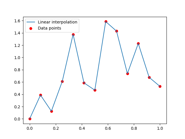
(a) Linear interpolation illustration

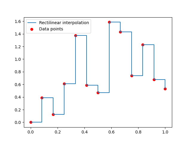
(b) Rectilinear interpolation illustration

Figure 1: Common embeddings

In the sequel, we will only use the linear embedding as this choice doesn’t seem to have a material impact on the information contained in the obtained signature as shown by the comparative study led by Fermanian (section 4.2 of Fermanian, 2021).

3.1.2 Extracting information of a one-dimensional process

Remember that if $X$ is a one-dimensional bounded variation path, then its signature over $[0,T]$ is equal to the powers of the increment $X_{T}-X_{0}$. As a consequence, finer information than the global increment about the evolution of $X$ on $[0,T]$ is lost. In our applications, $X$ represents an economic quantity like the level of an equity index so in most cases it is a one-dimensional stochastic process. In order to nonetheless be able to capture finer information about the evolution of $X$ on $[0,T]$, one can apply a transformation to $X$ to recover a multi-dimensional path. The two most widely used transformations are the time transformation and the lead-lag transformation. The time transformation consists in considering the two-dimensional path $\hat{X}_{t}:t\mapsto(t,X_{t})$ instead of $t\mapsto X_{t}$. The lead-lag transformation has been introduced by Gyurkó et al. (2013) in order to capture the quadratic variation of a path in the signature. Let $X$ be a real-valued stochastic process and $0=t_{0}<t_{1/2}<t_{1}<\dots<t_{N-1/2}<t_{N}=T$ be a partition of $[0,T]$. The lead-lag transformation of $X$ on the partition $(t_{i/2})_{i=0,\dots,2N}$ is the two-dimensional path $t\mapsto(X_{t}^{lead},X_{t}^{lag})$ defined on $[0,T]$ where:

1. the lead process $t\mapsto X_{t}^{lead}$ is the linear interpolation of the points $(X^{lead}_{t_{i/2}})_{i=0,\dots,2N}$ with:

   $$X^{lead}_{t_{i/2}}=\left\{\begin{array}[]{ll}X_{t_{j}}&\text{if }i=2j\\ X_{t_{j+1}}&\text{if }i=2j+1\end{array}\right.$$ (3.1)

2. the lag process $t\mapsto X_{t}^{lag}$ is the linear interpolation of the points $(X^{lag}_{t_{i/2}})_{i=0,\dots,2N}$ with:

   $$X^{lag}_{t_{i/2}}=\left\{\begin{array}[]{ll}X_{t_{j}}&\text{if }i=2j\\ X_{t_{j}}&\text{if }i=2j+1\end{array}\right.$$ (3.2)

Illustrations of the lead and lag paths as well as the lead-lag transformation are provided in Figure 2.

Remark 3.1.

The choice of the dates $(t_{i+1/2})_{i=0,\dots,N-1}$ such that $t_{i}<t_{i+1/2}<t_{i+1}$ can be arbitrary since the signature is invariant by time reparametrization (see Proposition 4.3 in Section 4.2).

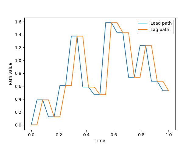
(a) Lead and lag paths

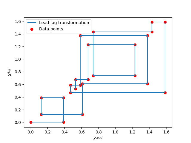
(b) Lead-lag transformation

Figure 2: Lead-lag illustrations

A third transformation can be constructed from the time and the lead-lag transformations. Indeed, given a finite set of observations $(X_{t_{i}})_{i=0,\dots,N}$, one can consider the three-dimensional path $t\mapsto(t,X_{t}^{lead},X_{t}^{lag})$. We call this transformation the time lead-lag transformation. Finally, the cumulative lead-lag transformation is the two-dimensional path $t\mapsto(\tilde{X}_{t}^{lead},\tilde{X}_{t}^{lag})$ where $\tilde{X}_{t}^{lead}$ (resp. $\tilde{X}_{t}^{lag}$) is the lead (resp. lag) transformation of the points $(\tilde{X}_{t_{i}})_{i=0,\dots,N+1}$ with:

$$\tilde{X}_{t_{i}}=\left\{\begin{array}[]{ll}0&\text{for $i=0$}\\ \sum_{k=0}^{i-1}X_{t_{k}}&\text{for $i=1,\dots,N+1$}.\end{array}\right.$$ (3.3)

This transformation has been introduced by Chevyrev and Kormilitzin (2016) because its signature is related to the statistical moments of the initial path $X$. More details on this point are provided in Remark 4.1 of Section 4.1.

3.1.3 Numerical computation of the signature and the MMD

The numerical computation of the signature is performed using the eSig Python package (version 0.9.8.3). Because the signature is an infinite object, we compute in practice only the truncated signature up to some specified order $R$. The influence of the truncation order on the statistical power of the test will be discussed in Section 3.2. Note that we will focus on truncation orders below 8 as there is not much information beyond this order given that we work with a limited number of observations of each path which implies that the approximation of high order iterated integrals will rely on very few points.

3.2 Analysis of the statistical power on synthetic data

In this subsection, we apply the signature-based validation on simulated data, i.e. the two samples of stochastic processes are numerically simulated. Keeping in mind insurance applications, the two-sample test is structured as follows:

• Each path is obtained by a linear interpolation from a set of 13 equally-spaced observations of the stochastic process under study. The first observation (i.e. the initial value of each path) is the same across all paths. These 13 observations represent monthly observations over a period of one year. In insurance practice, computational time constraints around the asset and liability models generally limit the simulation frequency to a monthly time step. The period of one year is justified by the fact that one needs to split the historical path under study into several shorter paths to get a test sample of size greater than 1. Because the number of historical data points is limited (about 30 years of data for the major equity indices), a split frequency of one year appears reasonable given the monthly observation frequency.

• The two samples are assumed to be of different sizes (i.e. $m\neq n$ with the notations of section 2.3). Several sizes $m$ of the first sample will be tested while the size $n$ of the second sample is always set to 1000. The first sample representing historical paths, we will mainly consider small values of $m$ as $m$ will in practice be equal to the number of years of available data (considering a split of the historical path in 1-year length paths as discussed above). For the second sample which consists in simulated paths (for example by an Economic Scenario Generator), we take 1000 simulated paths as it corresponds to a lower bound of the number of scenarios typically used by insurers. Numerical tests (not presented here) have also been performed with a sample size of 5000 instead of 1000 but the results were essentially the same.

• As we aim to explore the capability of the two-sample test to capture properties of the paths that cannot be captured by looking at their marginal distribution at some dates, we impose that the distributions of the increment over $[0,T]$ of the two compared stochastic processes are the same. In other words, we only compare stochastic processes $(X_{t})_{0\leq t\leq T}$ and $(Y_{t})_{0\leq t\leq T}$ satisfying $X_{T}-X_{0}\overset{\mathcal{L}}{=}Y_{T}-Y_{0}$ with $T=1$ year. This constraint is motivated by the fact that two models that do not have the same marginal one-year distribution are already discriminated by the current point-in-time validation methods. Moreover, it is a common practice in the insurance industry to calibrate the real-world models by minimizing the distance between model and historical moments so that the model marginal distribution is often close to the historical marginal distribution. Because of this constraint, we will remove the first order term of the signature in our estimation of the MMD because it is equal to the global increment $X_{T}-X_{0}$ and it does not provide useful statistical information.

In order to measure the ability of the signature-based validation to distinguish two different samples of paths, we compute the statistical power of the underlying test, which is the probability to correctly reject the null hypothesis under $H_{1}$, by simulating 1000 times two samples of sizes $m$ and $n$ respectively and counting the number of times that the null hypothesis (the stochastic processes underlying the two samples are the same) is rejected. The rejection threshold is obtained using the empirical Gram matrix spectrum as described in Section 2.3. First, we generate a sample of size $m$ and a sample of size $n$ under $H_{0}$ to compute the eigenvalues of the matrix $\hat{A}$ in Theorem 2.6. Then, we keep the 20 first eigenvalues in decreasing order and we perform 10000 simulations of the random variable in Equation (2.29) whose distribution approximates the MMD asymptotic distribution under $H_{0}$. The rejection threshold is obtained as the empirical quantile of level $99$% of these samples. For each experiment presented in the sequel, we also simulate 1000 times two samples of sizes $m$ and $n$ under $H_{0}$ and we count the number of times that the null hypothesis is rejected with this rejection threshold, which gives us the type I error. This step allows us to verify that the computed rejection threshold provides indeed a test of level $99$% in all experiments. As we obtain a type I error around 1% in all numerical experiments, we conclude to the accuracy of the computed rejection threshold.

We will now present numerical results for two stochastic processes: the fractional Brownian motion and the Black-Scholes dynamics as well as two time series models: an regime-switching $AR(1)$ process and a random walk with i.i.d. Gamma noises.

3.2.1 The fractional Brownian motion

The fractional Brownian motion (fBm) is a generalization of the standard Brownian motion that, outside this standard case, is neither a semimartingale nor a Markov process and whose sample paths can be more or less regular than those of the standard Brownian motion. More precisely, it is the unique centered Gaussian process $(B_{t}^{H})_{t\geq 0}$ whose covariance function is given by:

$$\mathbb{E}[B_{s}^{H}B_{t}^{H}]=\frac{1}{2}\left(s^{2H}+t^{2H}-(s-t)^{2H}\right)\quad\forall s,t\geq 0$$ (3.4)

where $H\in]0,1[$ is called the Hurst parameter. Taking $H=1/2$, we recover the standard Brownian motion. The fBm exhibits two interesting pathwise properties:

1. the fBm sample paths are $H-\epsilon$ Hölder for all $\epsilon>0$, that is

   $$\mathbb{P}\left(\sup_{s\neq t}\frac{\left|B_{t}^{H}-B_{s}^{H}\right|}{|t-s|^{H-\epsilon}}<\infty\right)=1\quad\forall\epsilon>0.$$ (3.5)

   Thus, when $H<1/2$, the fractional Brownian motion sample paths are rougher than those of the standard Brownian motion and when $H>1/2$, they are smoother.

2. the increments are correlated:

   $$\mathbb{E}[(B_{t}^{H}-B_{s}^{H})(B_{v}^{H}-B_{u}^{H})]=\frac{1}{2}\left(|s-v|^{2H}+|t-u|^{2H}-|t-v|^{2H}-|s-u|^{2H}\right)\quad\forall s,t,u,v\geq 0.$$ (3.6)

   In particular, if $s<t<u<v$, then $\mathbb{E}[(B_{t}^{H}-B_{s}^{H})(B_{v}^{H}-B_{u}^{H})]$ is positive if $H>1/2$ and negative if $H<1/2$ since $x\mapsto x^{2H}$ is convex if $H>1/2$ and concave otherwise.

One of the main motivations for studying this process is the work of Gatheral et al. (2018) which shows that the historical volatility of many financial indices essentially behaves as a fBm with a Hurst parameter around 10%.

In the following numerical experiments, we will compare samples from a fBm with Hurst parameter $H$ and samples from a fBm with a different Hurst parameter $H^{\prime}$. One can easily check that $B_{1}^{H}$ has the same distribution than $B_{1}^{H^{\prime}}$ since $B_{1}^{H}$ and $B_{1}^{H^{\prime}}$ are both standard normal variables. Thus, the constraint that both samples have the same one year marginal distribution (see the introduction of Section 3.2) is satisfied. Note that a variance rescaling should be performed if one considers a horizon that is different from 1 year. We start with a comparison of fBm paths having a Hurst parameter $H=0.1$ with fBm paths having a Hurst parameter $H=0.2$ using the lead-lag transformation. In Figure 3, we plot the statistical power as a function of the truncation order $R$ for different values of the first sample size $m$ (we recall that the size of the second sample is fixed to 1000).

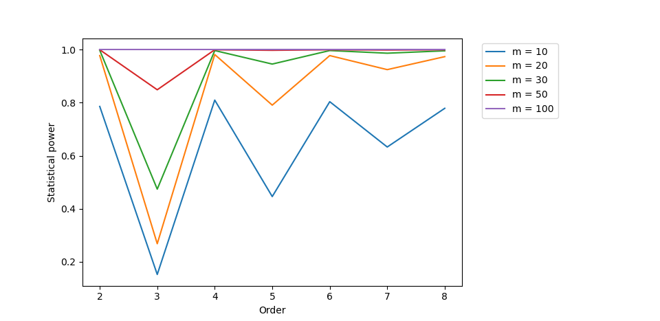
Figure 3: Statistical power of the signature-based validation test ($H=0.1$ versus $H^{\prime}=0.2$) as a function of the truncation order

We observe that even with small sample sizes, we already obtain a power close to 1 at order 2. Note that the power does not increase with the order but decreases at odd orders when the sample size is smaller than 50. This can be explained by the fact that the odd-order terms of the signature of the lead-lagged fBm are linear combinations of monomials in $B_{t_{1}}^{H},\dots,B^{H}_{t_{N}}$ that are of odd degree. Since $(B_{t}^{H})$ is a centered Gaussian process, the expectation of these terms are zero no matter the value of $H$. As a consequence, the contribution of odd-order terms of the signature to the MMD is the same under $H_{0}$ and under $H_{1}$. This is formalized in Proposition E.1 of Appendix E. Moreover, if we compute $MMD_{m,n}$ by keeping only one specific order of the signature and we estimate the power of the associated test, we obtain Table 2 which is consistent with the above explanation.

m \Order	2	3	4	5	6	7	8
10	79.4%	9.9%	81.5%	15.3%	80.4%	23.0%	78.1%
20	97.7%	9.8%	98.1%	18.7%	98.0%	28.8%	97.5%
30	99.7%	10.7%	99.7%	20.8%	99.7%	29.8%	99.6%
50	100.0%	9.7%	100.0%	20.7%	100.0%	33.4%	100.0%
100	100.0%	8.4%	100.0%	20.6%	100.0%	34.7%	100.0%
150	100.0%	9.6%	100.0%	21.8%	100.0%	33.4%	100.0%

Table 2: Statistical power of the signature-based validation test ($H=0.1$ versus $H^{\prime}=0.2$) restricted to one order.

If we conduct the same experiment for $H=0.1$ versus $H^{\prime}=0.5$ (corresponding to the standard Brownian motion), we obtain cumulated powers greater than 99% for all tested orders and sample sizes (even $m=10$) even if the power of the odd orders is small (below 45%). This is very promising as it shows that the signature-based validation allows to distinguish very accurately rough fBm paths (with a Hurst parameter in the range of those estimated by Gatheral et al., 2018) from standard Brownian motion paths even with small sample sizes.

Note that in these numerical experiments, we have not used any tensor normalization while it is a key ingredient in Theorem 2.3. This is motivated by the fact that the power is much worse when we use Chevyrev and Oberhauser’s normalization (described in Appendix D.1) as one can see on Figure 4. These lower powers can be understood as a consequence of the fact that the normalization is specific to each path. So the normalization can bring the distribution of $S(\hat{B}^{H^{\prime}})$ closer to the one of $S(\hat{B}^{H})$ than without normalization so that it is harder to distinguish them at fixed sample size. Moreover, if the normalization constant $\lambda$ is smaller than 1 (which we observe numerically), the high-order terms of the signature become close to zero and their contribution to the MMD is not material. For $H=0.1$ versus $H^{\prime}=0.5$, we observed that the powers remain very close to 100%.

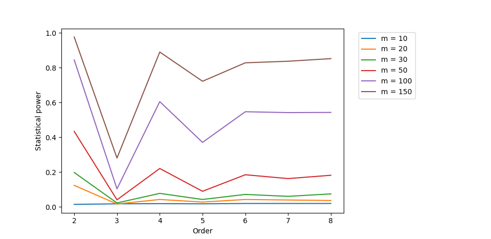
Figure 4: Statistical power of the normalized signature-based validation test ($H=0.1$ versus $H^{\prime}=0.2$) as a function of the truncation order

Also note that the lead-lag transformation is key for this model as replacing it by the time transformation (see Section 3.1.2) results in much lower statistical powers, see Figure 5. This observation is consistent with the previous study from Fermanian (2021) which concluded that the lead-lag transformation is the best choice in a learning context.

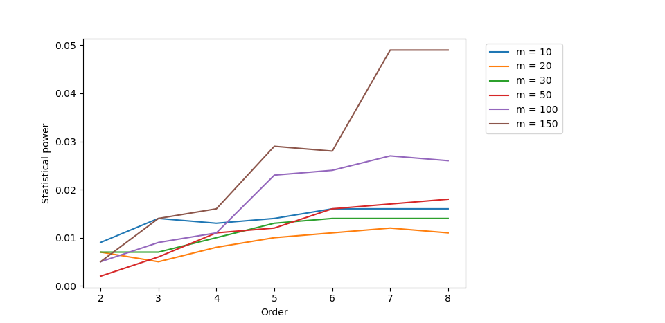
Figure 5: Statistical power of the signature-based validation test ($H=0.1$ versus $H^{\prime}=0.2$) as a function of the truncation order when using the time transformation

Before moving to the Black-Scholes dynamics, we present results of the test when the signature is replaced by the log-signature. The log-signature is a more parsimonious - though equivalent - representation of paths than the signature as it contains more zeros. A formal definition of the log-signature and more insights can be found in Section 4. Although no information is lost by the log-signature, it is not clear whether the MMD is still a metric when the signature is replaced by the log-signature in the kernel (see Remark 4.5 in Section 4). Numerically, the log-signature shows satisfying powers for $H=0.1$ versus $H^{\prime}=0.2$, especially when the truncation order is 2 (see Figure 6). One can remark in particular that the power decreases with the order. This observation likely results from the $1/n$ factor appearing in the log-signature formula (equation (4.22) in Section 4) which makes high-order terms of the log-signature small so that the even-order terms no longer compensate the odd-order terms. Note that in terms of CPU time, the log-signature is approximately 2.5 times faster to compute than the signature (0.35 ms to compute the log-signature of one path and 0.9 ms for the signature with a standard laptop with a 1.8 GHz processor) because of the fact that they are less coefficients to compute in the log-signature than in the signature. Therefore, the log-signature could be preferred to the signature if the CPU time is a constraint in practical applications.

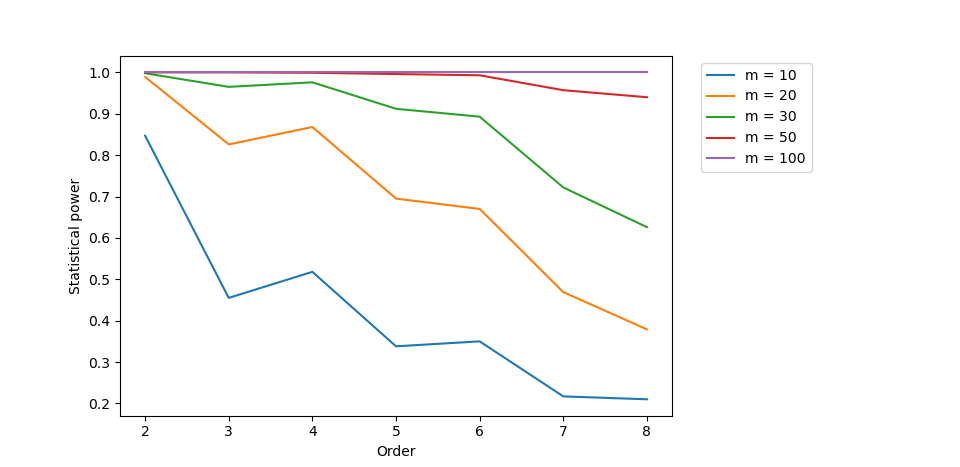
Figure 6: Statistical power of the log-signature-based validation test ($H=0.1$ versus $H^{\prime}=0.2$) as a function of the truncation order

3.2.2 The Black-Scholes dynamics

In the well-known Black-Scholes model (Black and Scholes, 1973), the evolution of the stock price $(S_{t})_{t\geq 0}$ is modelled using the following dynamics:

$$dS_{t}=\mu S_{t}dt+\sigma_{t}S_{t}dW_{t},\quad S_{0}=s_{0}$$ (3.7)

where $\mu\in\mathbb{R}$, $\sigma$ is a deterministic function of time and $(W_{t})_{t\geq 0}$ is a standard Brownian motion. Because of its simplicity, this model is still widespread in the insurance industry, in particular for the modelling of equity and real estate indices.

As for the fractional Brownian motion, we want to compare two parametrizations of this model that share the same one year marginal distribution. For this purpose, we consider a Black-Scholes dynamics (BSd) with drift $\mu$ and constant volatility $\sigma$ and a BSd with the same drift $\mu$ but with a deterministic volatility $\gamma(t)$ satisfying $\int_{0}^{1}\gamma^{2}(s)ds=\sigma^{2}$ which guarantees that the one-year marginal distribution constraint is met. For the sake of simplicity, we take a piecewise constant volatility with $\gamma(t)=\gamma_{1}$ if $t\in[0,1/2)$ and $\gamma(t)=\gamma_{2}$ if $t\in[1/2,1]$. In this setting, the objective of the test is no longer to distinguish two stochastic processes with different regularity but two stochastic processes with different volatility which is a priori more difficult since the volatility is not directly observable in practice. When $\mu=0$, the first two terms of the signature of the lead-lag transformation have the same asymptotic distribution in the two parametrizations as the time step converges to 0. This is explained in Example 4.3 in Section 4.1. We conjecture that this result extends to the full signature so that the two models cannot be distinguished using the signature.

We start by comparing BSd paths with $\mu=0.05$ and $\sigma=0.2$ and BSd paths with $\mu=0.05$, $\gamma_{1}=0$ and $\gamma_{2}=\sqrt{2}\sigma$ using the lead-lag transformation. We consider a zero volatility on half of the time interval in order to obtain very different paths in the two samples. Despite this extreme parametrization, we obtain very low powers as shown in Figure 7, even for larger sample sizes. It seems that the constraint of same quadratic variation in both samples makes the signatures from sample 1 too close from those of sample 2.

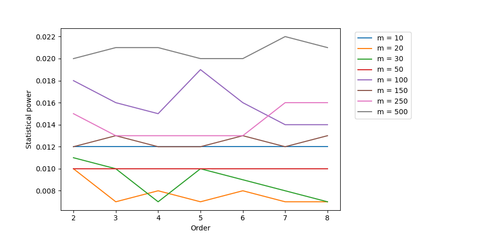
Figure 7: Statistical power of the signature-based validation test (constant volatility BSd versus piecewise constant volatility BSd) as a function of the truncation order.

In order to improve the power of the test, we can consider another data transformation which allows to capture information about the initial one-dimensional path in a different manner. We observed that the time lead-lag transformation (see Section 3.1.2) allowed to better distinguish the signatures from the two parametrizations given above. However, the order of magnitude of the differentiating coefficients of the signature (i.e. the coefficients of the signature that are materially different between the two samples) was significantly smaller than the one of non-differentiating coefficients so that the former were hidden by the latter when computing $MMD_{m,n}$. To address this issue, we applied a rescaling to all coefficients of the signature to make sure they are all of the same order of magnitude. Concretely, given two samples $\mathcal{S}_{1}=\{X_{1},\dots,X_{m}\}$ and $\mathcal{S}_{2}=\{Y_{1},\dots,Y_{n}\}$ of $d$-dimensional paths, the rescaling is performed as follows:

1. for all $i\in\{1,\dots,m\}$ and for all $j\in\{1,\dots,n\}$, compute $S(X_{i})$ and $S(Y_{j})$

2. for all $\ell\in\{1,\dots,R\}$ and for all $I=(i_{1},\dots,i_{\ell})\in\{1,\dots,d\}^{\ell}$, compute

   $$M_{I}^{\ell}=\max\left(\max_{i=1,\dots,m}\left|\mathbf{X}^{\ell}_{i,I}\right|,\max_{j=1,\dots,n}\left|\mathbf{Y}^{\ell}_{j,I}\right|\right)$$ (3.8)

   where $\mathbf{X}^{\ell}_{i,I}$ (resp. $\mathbf{Y}^{\ell}_{j,I}$) is the coefficient at position $I$ of the $\ell$-th term of the signature of $X_{i}$ (resp. $Y_{j}$).

3. for all $i\in\{1,\dots,m\}$, for all $j\in\{1,\dots,n\}$, for all $\ell\in\{1,\dots,R\}$ and for all $I=(i_{1},\dots,i_{\ell})\in\{1,\dots,d\}^{\ell}$, compute the rescaled signature as:

   $$\mathbf{\hat{X}}^{\ell}_{i,I}=\frac{\mathbf{X}^{\ell}_{i,I}}{M_{I}^{\ell}}\quad\text{and}\quad\mathbf{\hat{Y}}^{\ell}_{j,I}=\frac{\mathbf{Y}^{\ell}_{j,I}}{M_{I}^{\ell}}.$$ (3.9)

This procedure guarantees that all coefficients of the signature lie within $[-1,1]$. Using this normalization for the time lead-lag rescaling, the power of the test is significantly better than with the plain lead-lag transformation, as shown in Figure 8(a). In Figure 8(b), we show that the power can be further improved by considering the log-signature instead of the signature. Note that the increase of the power starts at order 3 which makes sense since order 2 only allows to capture the quadratic variation over $[0,T]$ (which is the same in the two parametrizations) while order 3 allows to capture the evolution of the quadratic variation over time. Alternatively, one can consider, instead of the time lead-lag transformation, the cumulative lead-lag transformation (see Equation (3.3) which provides even better statistical powers as shown in Figure 9.

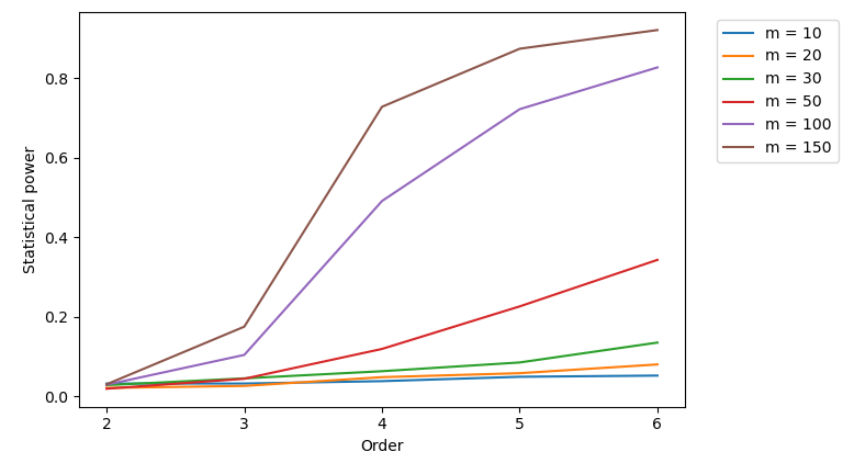
(a) With the signature

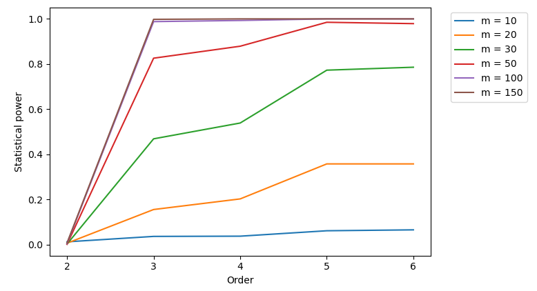
(b) With the log-signature

Figure 8: Statistical power of the validation test (constant volatility BSd versus piecewise constant volatility BSd) as a function of the truncation order when using the time lead-lag transformation with the rescaling procedure.

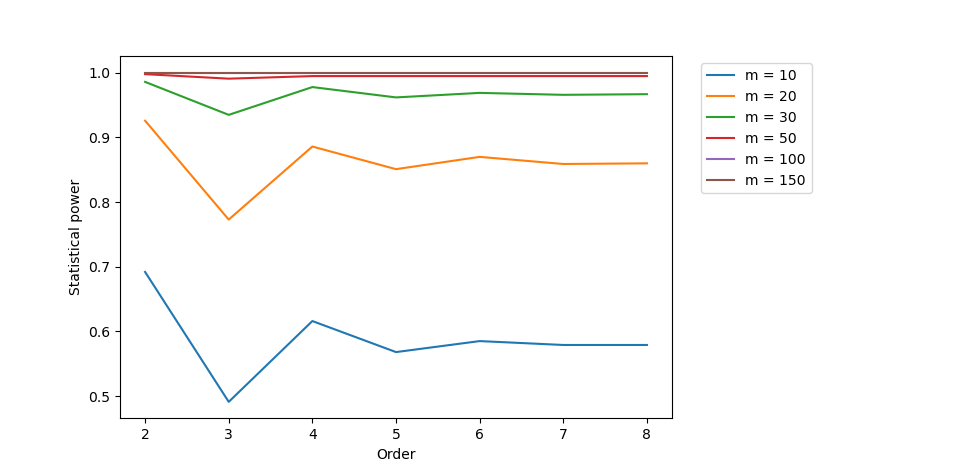
Figure 9: Statistical power of the signature-based validation test (constant volatility BSd versus piecewise constant volatility BSd) as a function of the truncation order using the cumulative lead-lag transformation on the log-paths.

We also considered a slight variation of the BSd that has autocorrelation. Let $(t_{i})_{0\leq i\leq N}$ be an equally-spaced partition of $[0,1]$ with $\Delta t=t_{i+1}-t_{i}=1/N$. The autocorrelated discretized BSd $(S^{C}_{t_{i}})_{0\leq i\leq N}$ is defined as follows:

$$\left\{\begin{array}[]{rcll}S^{C}_{t_{i+1}}&=&S^{C}_{t_{i}}\exp\left((\mu^{C}-\frac{\gamma_{t_{i}}^{2}}{2})\Delta t+\gamma_{t_{i}}\sqrt{\Delta t}G_{i+1}\right),&i\in\{0,\dots,N-1\}\\ S^{C}_{t_{0}}&=&s_{0}&\end{array}\right.$$ (3.10)

where $(G_{i})_{1\leq i\leq N}$ is a sequence of standard normal random variables satisfying:

$$Cov(G_{i},G_{j})=\left\{\begin{array}[]{ll}1&\text{if }i=j\\ \rho&\text{if }|i-j|=1\\ 0&\text{otherwise.}\end{array}\right.$$ (3.11)

The covariance matrix of $(G_{1},\dots,G_{N})$ is positive definite when $\rho\in\left(-\frac{1}{2\cos\left(\frac{\pi}{N+1}\right)},\frac{1}{2\cos\left(\frac{\pi}{N+1}\right)}\right)$. Indeed, the covariance matrix is a tridiagonal Toepliz matrix so its eigenvalues are given by (page 59 in Smith, 1985):

$$\lambda_{k}=1+2\rho\cos\left(\frac{k\pi}{N+1}\right),\quad k=1,\dots,N.$$ (3.12)

In our framework, we have $N=12$ and we can check that $[-0.5,0.5]\subset\left(-\frac{1}{2\cos\left(\frac{\pi}{N+1}\right)},\frac{1}{2\cos\left(\frac{\pi}{N+1}\right)}\right)$. In Figure 10, we compare BSd paths with $\mu=0.05$ and $\sigma=0.2$ and autocorrelated BSd paths with correlation $\rho\in\{-0.5,-0.4,\dots,0.5\}$ and a piecewise constant volatility like in the previous setting but with $\gamma_{1}=\sigma/\sqrt{2}$ and $(\gamma_{2},\mu^{C})$ chosen such that $S^{C}_{1}$ has the same distribution as $s_{0}e^{\mu-\sigma^{2}/2+\sigma W_{1}}$. Here, the first sample size is fixed to $m=30$. While it was not possible to distinguish BSd paths with different volatility functions using the lead-lag transformation, we observe that the introduction of autocorrelation makes the distinction again possible even with a small sample size. More precisely, except if $\rho\in\{-0.1,0,0.1,0.2\}$, we obtain a power greater than 90% at order 2. We note however a decrease of the power with the truncation order as it appears that apart from the term of order 2, all the other terms of the signature are very close between the two samples.

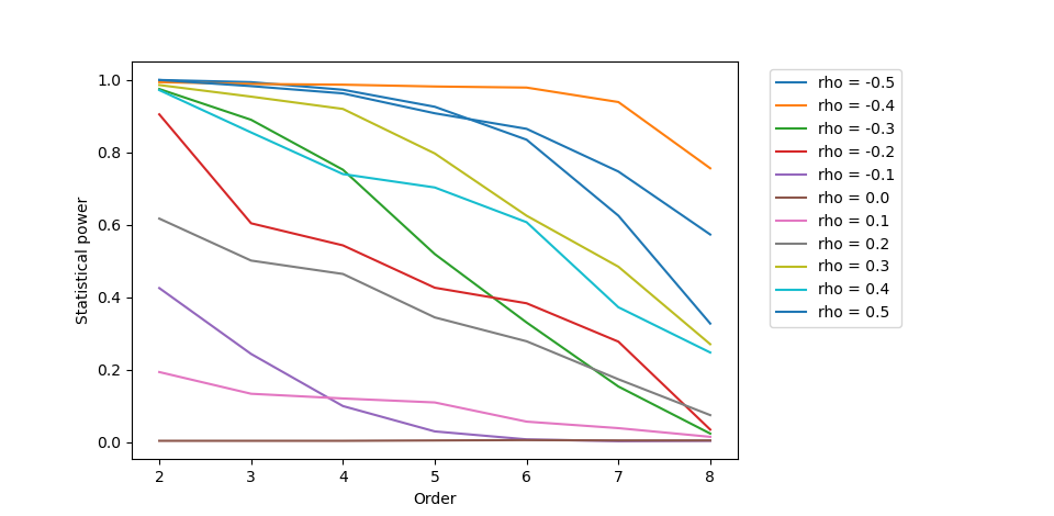
Figure 10: Statistical power of the log-signature-based validation test (constant volatility BSd versus autocorrelated BSd) as a function of the truncation order when using the lead-lag transformation with the rescaling procedure.

3.2.3 Time series models

The models presented in this section are inspired by models being used in the insurance industry to model inflation. Let us denote by $I_{t}$ the value of an inflation index (e.g. the Consumer Price Index) at time $t$ and by $X_{t}=\log\frac{I_{t}}{I_{t-\Delta}}$ the log-return of this index over a time interval of size $\Delta$. The first model under study assumes that the log-returns evolve as a regime-switching $AR(1)$ process:

$$X_{t+\Delta}=\mu_{S_{t+\Delta}}+\phi_{S_{t+\Delta}}(X_{t}-\mu_{S_{t+\Delta}})+\sigma_{S_{t+\Delta}}\epsilon_{t+\Delta}$$ (3.13)

where $X_{0}$ is fixed and $S$ is a time-homogeneous discrete Markov chain with $K\geq 2$ states and whose transition matrix is denoted by $P$. The noises $(\epsilon_{t})_{t\geq 0}$ are assumed to be i.i.d. standard normal variables. The second model under study assumes that the log-returns are i.i.d. non-centered Gamma noises whose shift, shape and scale parameters are respectively denoted by $\gamma$, $\alpha$ and $\beta$. In the following, we refer to this model as the Gamma random walk.

Note that for the regime-switching $AR(1)$ process, the annual log-return $\log\frac{I_{1}}{I_{0}}$ is distributed according to a Gaussian mixture while for the Gamma random walk, the annual log-return is Gamma distributed. Therefore, in order to still have close distributions for the annual log-return between the two models, we choose the parameters of the models so that the three first moments of the annual log-return are the same in both models. This is made possible by the fact that we can compute all moments in both cases and the fact that the parameters $\gamma$, $\alpha$ and $\beta$ of the Gamma noises $\epsilon_{t}$ can be explicitly written as a function of the three first moments of $\epsilon_{t}$ (see section 17.7 of Johnson et al., 1994). Therefore, given $X_{0}$, $(\mu_{i})_{1\leq i\leq K}$,$(\phi_{i})_{1\leq i\leq K}$, $(\sigma_{i})_{1\leq i\leq K}$ and $P$, we can find $\gamma$, $\alpha$ and $\beta$ such that the three first moments of the annual log-return are matched. In Figure 11, the distributions of the annual log-return are compared for the parameters reported in Table 3. We observe that they are close which is confirmed by a two-sample Kolmogorov-Smirnov test (applied on 1000 simulated one-year monthly paths of each model) yielding a $p$-value of 0.50.

	$X_{0}$	$\mu_{1}$	$\mu_{2}$	$\phi_{1}$	$\phi_{2}$	$\sigma_{1}$	$\sigma_{2}$	$P$
Regime-switching $AR(1)$	0	0.002	0.006	0.45	0.6	0.0025	0.004	$\begin{pmatrix}0.95&0.05\\ 0.1&0.9\end{pmatrix}.$
	$\gamma$	$\alpha$	$\beta$
Gamma random walk	-0.6880	0.4734	1.4534

Table 3: Parameters of the two models. The parameters of the regime-switching $AR(1)$ process are inspired from parameters calibrated on real inflation data that we present later while the parameters of the Gamma random walk are obtained by moment-matching as described above.

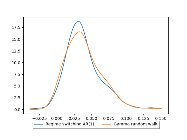
Figure 11: Kernel-density estimates of annual log-returns using Gaussian kernels. The annual log-returns are obtained by simulating 1000 one-year monthly paths of each model.

In Figure 12, we plot the statistical power of the two-sample test using the lead-lag transformation and the log-signature for an $AR(1)$ process with two regimes and for a Gamma random walk. The parameters of both models are given in Table 3. Note that the regime at $t=0$ is sampled from the stationary distribution of the Markov chain. We obtain statistical powers that are very close to 1 at any order for a sample size greater than $m=30$. This third case shows that the signature-based validation test is still powerful when working with time series models and allows to distinguish between paths exhibiting changes of regimes over time and first-order autocorrelation from paths with i.i.d. log-returns. Note that we have performed the same experiment with a regime-switching random walk (i.e. $\phi_{1}=\phi_{2}=0$) instead of a regime-switching $AR(1)$ process and we obtained statistical powers above 88% for a sample size greater than $m=50$ which shows that the first-order autocorrelation component is not necessary to distinguish the two models.

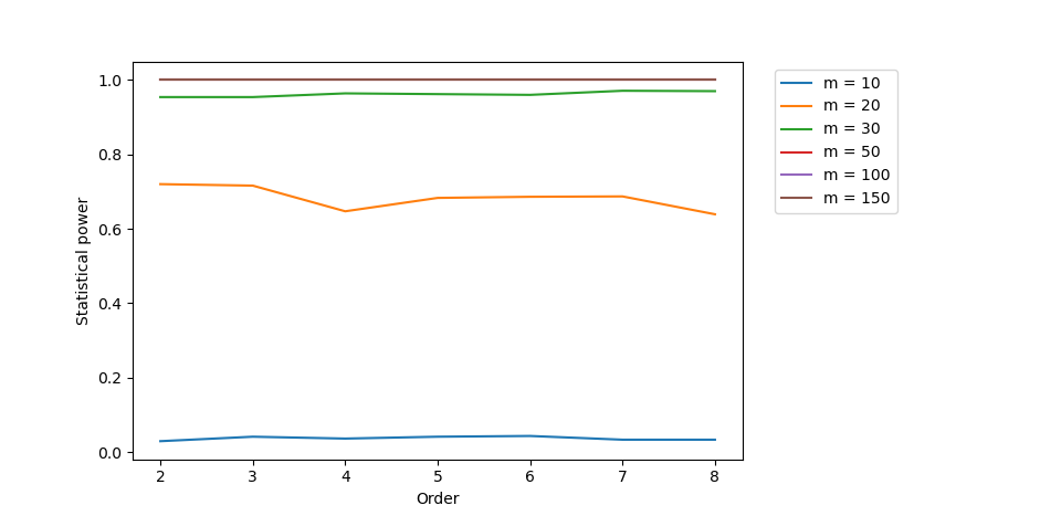
Figure 12: Statistical power of the log-signature-based validation test (regime-switching $AR(1)$ versus Gamma random walk) as a function of the truncation order when using the lead-lag transformation.

3.3 Application to historical data

The purpose of this subsection is to show that the signature-based validation test is able to discriminate between stochastic models calibrated on historical data. This is of practical interest for the validation task of real-world economic scenarios but more generally it is of interest for academics or practitioners that would like to compare a new model to existing ones based on a criteria of consistency with historical data. We consider two data sets (illustrated in Figure 13):

1. Daily realized variance estimates of the S&P 500 from January 2000 to January 2022 obtained from the Oxford-Man Institute of Quantitative Finance (2023).

2. Monthly observations of the Consumer Price Index for All Urban Consumers (CPI-U) in the United States from January 1950 to November 2022 obtained from the U.S. Bureau of Labor Statistics (2023).

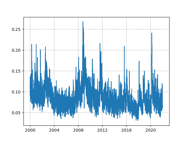
(a) Daily log-volatility of the the S&P 500 from January 2000 to January 2022.

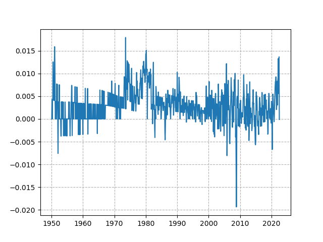
(b) Monthly log-returns of the Consumer Price Index for All Urban Consumers (CPI-U) in the United States from January 1950 to November 2022. Note that between 1950 and the beginning of 70s, the smaller precision in the measurement of the inflation index leads to monthly log-returns that seem to oscillate between some fixed values.

Figure 13: Data sets illustrations.

On the log-volatilities derived from the first data set, we calibrate an ordinary Ornstein-Uhlenbeck process and a fractional Ornstein-Uhlenbeck process whose dynamics is recalled below:

$$dY_{t}=\alpha(\theta-Y_{t})dt+\sigma dW_{t}^{H}$$ (3.14)

where $(W_{t}^{H})_{t\geq 0}$ is a fractional Brownian motion with Hurst parameter $H$. The ordinary Ornstein-Uhlenbeck process (corresponding to $H=1/2$ in Equation 3.14) is calibrated using the maximum likelihood estimators while the fractional Ornstein-Uhlenbeck process is calibrated using a two-step method. First, the Hurst parameter and the volatility parameter are estimated using the approach of Gatheral et al. (2018). Second, the mean-reversion speed and level are estimated using the method-of-moments estimators from Wang et al. (2019).

	$\theta$	$\alpha$	$\sigma$
Ornstein-Uhlenbeck	-5.0132	90.7993	8.2209
	$H$	$\theta$	$\alpha$	$\sigma$
Fractional Ornstein-Uhlenbeck	0.0916	-5.0131	0.2383	0.7876
	$\gamma$	$\alpha$	$\beta$
Gamma random walk	-0.00047	0.18208	0.01832
	$\mu_{1}$	$\mu_{2}$	$\phi_{1}$	$\phi_{2}$	$\sigma_{1}$	$\sigma_{2}$	$P$
Regime-switching AR(1)	0.0022	0.0062	0.4622	0.5774	0.0025	0.0042	$\begin{pmatrix}0.987&0.013\\ 0.0637&0.9363\end{pmatrix}$

Table 4: Calibrated parameters.

On the second data set, we calibrate a Gamma random walk and a regime-switching AR(1) process. The Gamma random walk is calibrated by matching the three first moments of the historical annual log-returns while the regime-switching AR(1) process is calibrated by log-likelihood maximization. The calibrated parameters are reported in Table 4. Note that the decrease in the $\alpha$ value between the ordinary and the fractional Ornstein-Uhlenbeck models results from the rough noise in latter model ($H<1/2$) that already captures a part of the negative autocorrelation.

For all models, we simulate 10000 one-year paths with a monthly frequency and we check that the simulated annual log-returns are close to the historical ones both graphically and using the two-sample Kolmogorov-Smirnov test. The plotted densities in Figure 14 appear reasonably close and the hypothesis of same distribution is not rejected by the Kolmogorov-Smirnov test for all models (see Table 5).

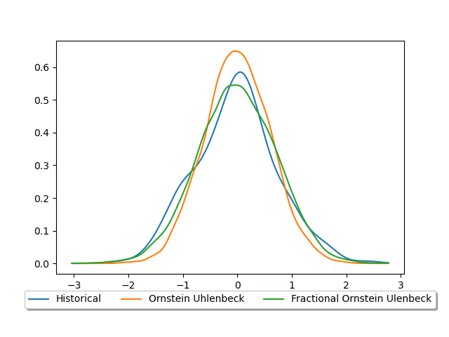
(a) First data set.

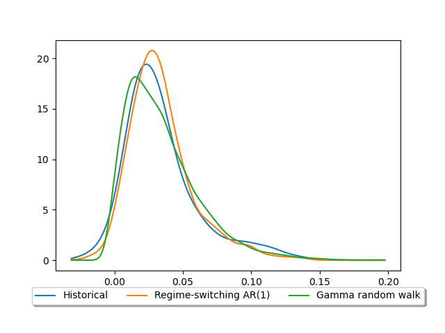
(b) Second data set.

Figure 14: Kernel-density estimates of annual log-returns using Gaussian kernels. The historical annual log-returns are computed using a one-year window which is moved with a monthly step for the first data set and with a quarterly step for the second data set.

First data set
	Ornstein-Uhlenbeck	Fractional Ornstein-Uhlenbeck
KS test $p$-value	0.09654	0.6544
Second data set
	Gamma random walk	Regime-switching AR(1)
KS test $p$-value	0.1302	0.1227

Table 5: $p$-value of the two-sample Kolmogorov-Smirnov test applied to historical annual log-returns and simulated annual log-returns for each model. The historical annual log-returns are computed using a one-year window which is moved with a monthly step for the first data set and with a quarterly step for the second data set.

In order to be able to apply the signature-based validation test, we construct one-year "historical paths" with a monthly frequency from the monthly observations $(X_{t_{i}})_{0\leq i\leq N}$ of each data set (for the first data set with a daily frequency, we keep the last value of each month) as follows: we split the observations $(X_{t_{i}})_{0\leq i\leq N}$ into $m=\lfloor N/12\rfloor$ groups of length 13 where the $k$-th group for $k\in\{0,\dots,m-1\}$ consists of $X_{t_{12k}}$, $X_{t_{12k+1}}$, $\dots$, $X_{t_{12(k+1)}}$. For the first data set, we have $m=22$ while for the second we have $m=72$, note that both lie in the range studied in the previous subsection. Moreover, we take the logarithm of the observations to be consistent with the models that work on the log-volatilities for the first data set and the log-returns for the second data set. Then, for each model, we compare 1000 simulated sample paths to these historical paths using the signature-based validation. The simulated paths start from $\theta$ for the ordinary and the fractional Ornstein-Uhlenbeck models and from 0 for the Gamma random walk and the regime-switching $AR(1)$ process. The initial regime for the regime-switching $AR(1)$ process is sampled from the stationary distribution of the Markov chain. The $p$-value of each test, obtained by computing $1-\hat{F}_{H_{0}}(\hat{MMD}^{2}_{m,n})$ where $\hat{F}_{H_{0}}$ is the empirical cumulative distribution function of $MMD_{m,n}^{2}$ under $H_{0}$ and $\hat{MMD}^{2}_{m,n}$ is the test statistic value, is reported in Table 6.

First data set
	Ornstein-Uhlenbeck	Fractional Ornstein-Uhlenbeck
Signature-based validation test $p$-value	0.0000	0.2362
Second data set
	Gamma random walk	Regime-switching AR(1)
Signature-based validation test $p$-value	0.0000	0.6956

Table 6: $p$-value of the signature-based validation test applied to historical paths and simulated paths for each model. For the first data set, the signature is truncated at order 4 and the lead-lag transformation is applied. For the second data set, the log-signature is truncated at order 4 and the lead-lag transformation is applied. In both cases, the term of order 1 of the signature/log-signature is removed because it is not very informative given that the increments in both models have close distributions.

We observe on the first data set that the ordinary Ornstein-Uhlenbeck model is rejected at any level while the fractional Ornstein-Uhlenbeck is not. This result shows using a different method than Gatheral et al. (2018) that volatility is rough. On the second data set, we observe that the Gamma random walk is rejected at any level while the regime-switching $AR(1)$ process is not. This is particularly interesting given that the $p$-values of the two-sample Kolmogorov-Smirnov test reported in Table 5 are very close. Moreover, this result is in line with the empirical observation that the inflation dynamics exhibits roughly two regimes in the second data set (see Figure 13): a regime of low inflation (e.g. between 1982 and 2021) and a regime of high inflation (e.g. between 1972 and 1982).

3.4 Numerical results summary

In this section, we have first presented the statistical power of the signature-based validation test in three different settings. In each of these settings, we have shown that high statistical powers can be achieved even in a small sample configuration and with a constraint on the closeness of the compared paths by using the following levers:

1. a transformation (lead-lag, time lead-lag, cumulative lead-lag) is applied to the path before taking the signature;

2. several truncation orders are tested;

3. the signature and the log-signature are compared;

4. a rescaling of the terms of the signature can be applied.

The combinations of these levers resulting in the highest statistical power over the tested sample sizes in the three settings are presented in Table 7.

Setting	Transformation	Order	Signature type	Rescaling
Fractional Brownian motion (Section 3.2.1)	Lead-lag	2	Log-signature	No
Black-Scholes dynamics (Section 3.2.2)	Cumulative lead-lag	2	Signature	No
Time series models (Section 3.2.3)	Lead-lag	No material influence	Log-signature	No

Table 7: Configurations of the two-sample test leading to the best statistical power.

Note that items 1, 3 and 4 are part of the generalized signature method introduced by Morrill et al. (2020) that aim at providing a unifying framework for the use of the signature as a feature in machine learning. A natural question at this stage is how to choose the transformation, truncation order, whether to use the signature or log-signature and whether to use a rescaling or not in a new setting that is not studied here. Unfortunately, we have not being able to find a general rule to make these choices especially because it does not seem possible to relate these choices to the properties of the models under study except in some cases we have exhibited above (e.g. even truncation order should be used for centered Gaussian processes). Therefore, we could suggest the following strategy to practitioners that would like to implement this validation test: use the test for every combination of the levers above and reject the null hypothesis if a majority of the tests is rejected. Applying this strategy for the two historical data sets leads to the same conclusions about the four studied models: the ordinary Ornstein-Uhlenbeck and the Gamma random walk are rejected while the fractional Ornstein-Uhlenbeck and the regime-switching $AR(1)$ process are not.

Second, we have shown that the signature-based validation test allows to reject some models while others are not rejected despite the fact that all produce annual log-returns that are reasonably close to the historical ones. This demonstrates that the signature is a promising tool to validate real-world models.

4 Examples and properties of the signature

The signature being already defined in Section 2.2, the purpose of this section is to provide more insights on the signature thanks to examples and a brief overview of its main properties.

4.1 Some examples

First, we present several examples that allow to better understand the signature and the log-signature.

Example 4.1.

If $X:[0,T]\rightarrow E$ is a linear path , i.e. $X_{t}=X_{0}+(X_{T}-X_{0})\frac{t}{T}$, then for any $n\geq 0$:

$$\mathbf{X}^{n}=\frac{1}{n!}(X_{T}-X_{0})^{\otimes n}.$$ (4.1)

Example 4.2.

If $E$ is a vector space of dimension 2, the second order term of the signature is given by:

$$\mathbf{X}^{2}=\int_{0}^{T}\int_{0}^{t}dX_{s}\otimes dX_{t}=\begin{pmatrix}\int_{0}^{T}\int_{0}^{t}dX_{s}^{(1)}dX_{t}^{(1)}&\int_{0}^{T}\int_{0}^{t}dX_{s}^{(1)}dX_{t}^{(2)}\\ \int_{0}^{T}\int_{0}^{t}dX_{s}^{(2)}dX_{t}^{(1)}&\int_{0}^{T}\int_{0}^{t}dX_{s}^{(2)}dX_{t}^{(2)}\end{pmatrix}.$$ (4.2)

Note that the difference of the anti-diagonal coefficients of $\mathbf{X}^{2}$ corresponds, up to a factor $1/2$, to the Lévy area of the curve $t\mapsto(X_{t}^{1},X_{t}^{2})$ which is defined as:

$$\mathcal{A}^{Levy}=\frac{1}{2}\left(\int_{0}^{T}(X_{t}^{1}-X_{0}^{1})dX_{t}^{2}-\int_{0}^{T}(X_{t}^{2}-X_{0}^{2})dX_{t}^{1}\right).$$ (4.3)

It is the signed area between the curve and the chord connecting the two endpoints (see Figure 15).

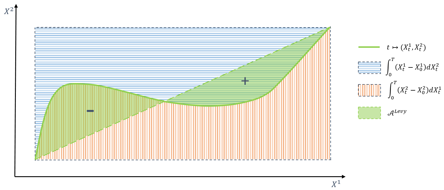
Figure 15: Illustration of the Lévy area. The blue dashed area corresponds to the integral $\int_{0}^{T}(X_{t}^{1}-X_{0}^{1})dX_{t}^{2}$ while the red dashed area corresponds to the integral $\int_{0}^{T}(X_{t}^{2}-X_{0}^{2})dX_{t}^{1}$. Taking the difference between these two areas yields the Levy area (represented in green transparent) up to a factor 2 because of a double counting. The ’$+$’ (resp. ’$-$’) sign indicates that the surrounding area is counted positively (resp. negatively).

In Section 3.1.2, we mentioned that the lead-lag transformation allows to capture the quadratic variation of a path in the signature. More precisely, the Levy area of the lead-lag transformation is the quadratic variation up to a factor $1/2$ as stated by the following proposition.

Proposition 4.1.

Let $t_{0}=0<t_{1}<\dots<t_{N}=T$ be a partition of $[0,T]$ and $(X_{t_{i}})_{i=0,\dots,N}$ be the vector of observations of a real-valued process $X$ on this partition. The Levy area of the lead-lag transformation of $(X_{t_{i}})_{i=0,\dots,N}$ is equal to the quadratic variation of $X$ on the partition $(t_{i})_{i=0,\dots,N}$ up to a factor $1/2$, i.e.

$$\frac{1}{2}\left(\int_{0}^{T}(X_{t}^{lead}-X_{0}^{lead})dX_{t}^{lag}-\int_{0}^{T}(X_{t}^{lag}-X_{0}^{lag})dX_{t}^{lead}\right)=\frac{1}{2}\sum_{i=0}^{N-1}(X_{t_{i+1}}-X_{t_{i}})^{2}.$$ (4.4)

Proof.

Using the notations introduced above, we have:

$$X_{t}^{lead}=\left\{\begin{array}[]{ll}X_{t_{i}}+\frac{X_{t_{i+1}}-X_{t_{i}}}{t_{i+1/2}-t_{i}}(t-t_{i})&\text{if }t\in[t_{i},t_{i+1/2}]\\ X_{t_{i+1}}&\text{if }t\in[t_{i+1/2},t_{i+1}]\end{array}\right.$$ (4.5)

and

$$X_{t}^{lag}=\left\{\begin{array}[]{ll}X_{t_{i}}&\text{if }t\in[t_{i},t_{i+1/2}]\\ X_{t_{i}}+\frac{X_{t_{i+1}}-X_{t_{i}}}{t_{i+1}-t_{i+1/2}}(t-t_{i+1/2})&\text{if }t\in[t_{i+1/2},t_{i+1}].\end{array}\right.$$ (4.6)

We deduce that,

$$\int_{0}^{T}(X_{t}^{lead}-X_{0}^{lead})dX_{t}^{lag} =\sum_{i=0}^{N-1}\int_{t_{i+1/2}}^{t_{i+1}}(X_{t_{i+1}}-X_{0})\frac{X_{t_{i+1}}-X_{t_{i}}}{t_{i+1}-t_{i+1/2}}dt$$

$$=\sum_{i=0}^{N-1}(X_{t_{i+1}}-X_{0})(X_{t_{i+1}}-X_{t_{i}})$$

$$=\sum_{i=0}^{N-1}\left[(X_{t_{i+1}}-X_{t_{i}})^{2}+(X_{t_{i}}-X_{0})(X_{t_{i+1}}-X_{t_{i}})\right].$$

A similar calculation yields

$$\int_{0}^{T}(X_{t}^{lag}-X_{0}^{lag})dX_{t}^{lead}=\sum_{i=0}^{N-1}(X_{t_{i}}-X_{0})(X_{t_{i+1}}-X_{t_{i}}).$$ (4.7)

Hence,

$$\int_{0}^{T}(X_{t}^{lead}-X_{0}^{lead})dX_{t}^{lag}-\int_{0}^{T}(X_{t}^{lag}-X_{0}^{lag})dX_{t}^{lead}=\sum_{i=0}^{N-1}(X_{t_{i+1}}-X_{t_{i}})^{2}.$$ (4.8)

∎

Remark 4.1.

We also mentioned in Section 3.1.2 that the cumulative lead-lag transformation $\tilde{X}$ of a sequence of observations $(X_{t_{i}})_{i=0,\dots,N}$ on $[0,T]$ can be related to the statistical moments of $X$. Indeed, the term of order 1 of the signature of $\tilde{X}$ is given by:

$$\tilde{\mathbf{X}}^{1}=\begin{pmatrix}\tilde{X}_{T}-\tilde{X}_{0}\\ \tilde{X}_{T}-\tilde{X}_{0}\\ \end{pmatrix}=\begin{pmatrix}\sum_{i=0}^{N}X_{t_{i}}\\ \sum_{i=0}^{N}X_{t_{i}}\\ \end{pmatrix}$$ (4.9)

which is the empirical mean of $X$ up to a factor $1/(N+1)$. From Proposition 4.1, we also deduce that the Levy area of the cumulative lead-lag transformation is given by:

$$\frac{1}{2}\sum_{i=0}^{N}(\tilde{X}_{t_{i+1}}-\tilde{X}_{t_{i}})^{2}=\frac{1}{2}\sum_{i=0}^{N}X_{t_{i}}^{2}$$ (4.10)

which is the empirical second order (non-central) moment of $X$ up to a factor $1/(N+1)$. More generally, the $n$-th (non-central) moment of $X$ can be obtained from the term of order $n$ of the signature of the cumulative lead-lag transformation.

We have seen in our numerical experiments in Section 3.2.2 that the lead-lag transformation is not always sufficient to distinguish models that are too close from a statistical perspective. In the following example, we show that, as the time step converges to 0, the first two terms of the signature of the lead-lag transformation of a driftless Black-Scholes dynamics with constant volatility have the same distributions as the first two terms of the signature of the lead-lag transformation of a driftless Black-Scholes dynamics with a time-dependent deterministic volatility if the total variances at time $T$ of both models are the same.

Example 4.3.

Consider $X$ and $Y$ the solutions of the following SDE’s

$$\begin{array}[]{rll}dX_{t}&=\sigma X_{t}dW_{t}&,X_{0}=1\\ dY_{t}&=\gamma(t)Y_{t}dW_{t}&,Y_{0}=1\end{array}$$ (4.11)

where $(W_{t})_{t\geq 0}$ is a Brownian motion and $\gamma$ is a deterministic function satisfying $\int_{0}^{T}\gamma(t)^{2}dt=\sigma^{2}T$. The explicit formulas of $X$ and $Y$ write:

$$X_{t} =\exp\left(\sigma W_{t}-\frac{1}{2}\sigma^{2}t\right)$$ (4.12)

$$Y_{t} =\exp\left(\int_{0}^{t}\gamma(s)dW_{s}-\frac{1}{2}\int_{0}^{t}\gamma(s)^{2}ds\right).$$

Let us denote by $\hat{X}_{N}$ (resp. $\hat{Y}_{N}$) the lead-lag transformation of $X$ (resp. $Y$) on a partition $(t_{i})_{i=0,\dots,N}$ of $[0,T]$ such that $t_{i}=iT/N$. The constraint $\int_{0}^{T}\gamma(t)^{2}dt=\sigma^{2}T$ implies that $X_{T}\overset{d}{=}Y_{T}$ so the first order terms of the signatures of $\hat{X}_{N}$ and $\hat{Y}_{N}$ (which reduce to the increments of $X$ and $Y$ over $[0,T]$) have the same distribution for all $N\geq 1$. The second order term of the signature of $\hat{Y}_{N}$ is given by (see the proof of the above proposition):

$$\hat{\mathbf{Y}}_{N}^{2}=\begin{pmatrix}\frac{1}{2}(Y_{T}-Y_{0})^{2}&\sum_{i=0}^{N-1}\left[(Y_{t_{i+1}}-Y_{t_{i}})^{2}+(Y_{t_{i}}-Y_{0})(Y_{t_{i+1}}-Y_{t_{i}})\right]\\ \sum_{i=0}^{N-1}(Y_{t_{i}}-Y_{0})(Y_{t_{i+1}}-Y_{t_{i}})&\frac{1}{2}(Y_{T}-Y_{0})^{2}\end{pmatrix}$$ (4.13)

Now, given that $Y$ is a square-integrable continuous martingale, the coefficient at position $(1,2)$ of $\hat{\mathbf{Y}}_{N}$ converges in probability as $N\to+\infty$ to:

$$\langle Y\rangle_{T}+\int_{0}^{T}(Y_{t}-Y_{0})dY_{t}=\frac{1}{2}\left[(Y_{T}-Y_{0})^{2}+\langle Y\rangle_{T}\right]$$ (4.14)

where $\langle Y\rangle$ denotes the quadratic variation process of $Y$ and the equality is obtained using the integration by parts formula. Similarly, the coefficient at position $(2,1)$ of $\hat{\mathbf{Y}}_{N}$ converges in probability as $N\to+\infty$ to:

$$\int_{0}^{T}(Y_{t}-Y_{0})dY_{t}=\frac{1}{2}\left[(Y_{T}-Y_{0})^{2}-\langle Y\rangle_{T}\right].$$ (4.15)

The same convergences hold for $\hat{\mathbf{X}}_{N}$. Now remark that the processes $\left(\int_{0}^{t}\gamma(s)dW_{s}\right)_{t\geq 0}$ and $\left(W_{\int_{0}^{t}\gamma(s)^{2}ds}\right)_{t\geq 0}$ are both Gaussian processes with the same mean and the same covariance function, we deduce that they have the same distribution. Analogously, $(\sigma W_{t})_{t\geq 0}$ has the same distribution as $(W_{\sigma^{2}t})$. We deduce that:

$$(X_{t})_{t\geq 0} \overset{d}{=}\left(\exp\left(W_{\sigma^{2}t}-\frac{1}{2}\sigma^{2}t\right)\right)_{t\geq 0}$$ (4.16)

$$(Y_{t})_{t\geq 0} \overset{d}{=}\left(\exp\left(W_{\int_{0}^{t}\gamma(s)^{2}ds}-\frac{1}{2}\int_{0}^{t}\gamma(s)^{2}ds\right)\right)_{t\geq 0}.$$

Setting $\varphi(t)=\frac{1}{\sigma^{2}}\int_{0}^{t}\gamma(s)^{2}ds$, we deduce that $(Y_{t})_{0\leq t\leq T}\overset{d}{=}(X_{\varphi(t)})_{0\leq t\leq T}$. As a consequence, $(Y_{t},\langle Y\rangle_{t})_{0\leq t\leq T}$ has the same distribution as $(X_{\varphi(t)},\langle X\rangle_{\varphi(t)}-\langle X\rangle_{\varphi(0)})_{0\leq t\leq T}$. Since $\varphi(0)=0$ and $\varphi(T)=T$, we conclude that the limit of $\hat{\mathbf{Y}}_{N}$ has the same distribution as the limit of $\hat{\mathbf{X}}_{N}$.

The log-signature

We now introduce more formally the log-signature. We recall that the space of formal series of tensors is defined as:

$$T(E)=\left\{(\mathbf{t}^{n})_{n\geq 0}\mid\forall n\geq 0,\mathbf{t}^{n}\in E^{\otimes n}\right\}$$ (4.17)

with the convention $E^{\otimes 0}=\mathbb{R}$. This space can be equipped with the following operations: for $\mathbf{t}$, $\mathbf{u}\in T(E)$, $\lambda\in\mathbb{R}$,

$$\begin{array}[]{rcl}\mathbf{t}+\mathbf{u}&=&(\mathbf{t}^{n}+\mathbf{u}^{n})_{n\geq 0}\\ \lambda\mathbf{t}&=&(\lambda\mathbf{t}^{n})_{n\geq 0}\\ \mathbf{t}\otimes\mathbf{u}&=&\left(\mathbf{v}^{n}=\sum_{k=0}^{n}\mathbf{t}^{k}\otimes\mathbf{u}^{n-k}\right)_{n\geq 0}.\end{array}$$ (4.18)

Since by convention the term of order 0 of the signature is set to 1, the signature takes its values in the following affine subspace of $T(E)$:

$$T_{1}(E)=\left\{\mathbf{t}\in T(E)\mid\mathbf{t}^{0}=1\right\}.$$ (4.19)

A closely related subspace of $T(E)$ is the following:

$$T_{0}(E)=\left\{\mathbf{t}\in T(E)\mid\mathbf{t}^{0}=0\right\}.$$ (4.20)

In fact, there is a bijection between $T_{1}(E)$ and $T_{0}(E)$ (Lemma 2.21 in Lyons et al., 2007):

Proposition 4.2.

Let us define the exponential mapping as:

$$\begin{array}[]{rcl}T_{0}(E)&\rightarrow&T_{1}(E)\\ \mathbf{t}&\mapsto&\exp(\mathbf{t}):=\displaystyle\sum_{n\geq 0}\frac{\mathbf{t}^{\otimes n}}{n!}\end{array}$$ (4.21)

with the convention $t^{\otimes 0}=1$ and the logarithm mapping as:

$$\begin{array}[]{rcl}T_{1}(E)&\rightarrow&T_{0}(E)\\ \mathbf{t}&\mapsto&\log(\mathbf{t}):=\displaystyle\sum_{n\geq 1}\frac{(-1)^{n-1}}{n}(\mathbf{t}-\mathbf{1})^{\otimes n}\end{array}$$ (4.22)

where $\mathbf{1}=(1,0,\dots,0,\dots)\in T_{1}(E)$. The exponential mapping is bijective from $T_{0}(E)$ to $T_{1}(E)$ and its inverse is the logarithm mapping.

Example 4.1 (continued).

Using the exponential and the logarithm mappings, we can rewrite the signature in Example 4.1 in the following way:

$$S(X)=\exp(X_{T}-X_{0})$$ (4.23)

where $X_{T}-X_{0}$ should be interpreted as the element $(0,X_{T}-X_{0},0,\dots,0,\dots)$ of $T_{0}(E)$. Moreover,

$$\log(S(X))=X_{T}-X_{0}.$$ (4.24)

Using the logarithm, it is therefore possible to define the log-signature of a path $X$ as $\log(S(X))$. Although there is a one-to-one correspondence between the signature and the log-signature, the log-signature is a more parsimonious representation of the path than the signature in the sense that it removes the redundancies. This can be seen in Example 4.1: the only non-zero term of the log-signature of a linear path is the term of order 1 which contains the increments of the path. In comparison to the signature, all the powers of the increments have disappeared. However, no information is lost. More generally, it can be shown (see for example Liao et al., 2019) that the log-signature has more zeros than the signature. As such, it represents a useful object for applications as it allows to avoid the exponential increase of the size of the truncated signature with the order. Indeed, if $E$ is a vector space of dimension $d$, the term of order $n$ of the signature has $d^{n}$ elements.

Example 4.4.

Let us consider $X\in\mathcal{C}^{1}([0,T],\mathbb{R}^{2})$. The second order term of the log-signature writes:

$$\mathbf{lX}^{2}=\mathbf{X}^{2}-\frac{1}{2}\mathbf{X}^{1}\otimes\mathbf{X}^{1}$$ (4.25)

where $\mathbf{X}^{2}$ comes from the first term ($n=1$) of the log series in Equation (4.22) and $\mathbf{X}^{1}\otimes\mathbf{X}^{1}$ comes from the second term ($n=2$). We have:

$$\mathbf{X}^{2}=\begin{pmatrix}\frac{(X_{T}^{1}-X_{0}^{1})^{2}}{2}&\int_{0}^{T}(X_{t}^{1}-X_{0}^{1})dX_{t}^{2}\\ \int_{0}^{T}(X_{t}^{2}-X_{0}^{2})dX_{t}^{1}&\frac{(X_{T}^{2}-X_{0}^{2})^{2}}{2}\end{pmatrix}$$ (4.26)

and

$$\mathbf{X}^{1}\otimes\mathbf{X}^{1}=\begin{pmatrix}(X_{T}^{1}-X_{0}^{1})^{2}&(X_{T}^{1}-X_{0}^{1})(X_{T}^{2}-X_{0}^{2})\\ (X_{T}^{1}-X_{0}^{1})(X_{T}^{2}-X_{0}^{2})&(X_{T}^{2}-X_{0}^{2})^{2}\end{pmatrix}.$$ (4.27)

Using the integration by part formula, we obtain:

$$\mathbf{lX}^{2}=\underbrace{\frac{1}{2}\left(\int_{0}^{T}(X_{t}^{1}-X_{0}^{1})dX_{t}^{2}-\int_{0}^{T}(X_{t}^{2}-X_{0}^{2})dX_{t}^{1}\right)}_{\text{L\'{e}vy area of $X$}}\begin{pmatrix}0&1\\ -1&0\end{pmatrix}$$ (4.28)

Hence, the second order term of the log-signature reduces to the Lévy area.

Remark 4.2.

Note that only the $N$ first terms of the logarithm series (4.22) contribute to the $N$-th term of the log-signature. Indeed, for $n>N$, the contributions to $E^{\otimes N}$ of $(\mathbf{t}-\mathbf{1})^{\otimes n}$ always involve some product by $(\mathbf{t}-\mathbf{1})^{0}=0$.

4.2 Properties

We have seen in the first subsection that the signature allows to capture some information about the path. A natural question at this stage is how much information about $X$ does the signature of $X$ contain. This subsection aims at answering this question.

Proposition 4.3 (Invariance under time reparametrization).

Let $X\in\mathcal{C}^{1}([0,T],E)$ and consider $\varphi:[0,T]\rightarrow[0,T]$ a non-decreasing surjection. If we set $\tilde{X}_{t}=X_{\varphi(t)}$, then:

$$S(\tilde{X})=S(X).$$ (4.29)

This first property (see Proposition 7.10 in Friz and Victoir, 2010 for a proof) means that the speed at which the path is traversed is not captured by the signature. The signature is also invariant by translation. Indeed, if we define $\bar{X}_{t}=x+X_{t}$, then $d\bar{X}_{t}=dX_{t}$ and by definition of the signature we have $S(\bar{X})=S(X)$. The next property we will outline is Chen’s identity. Before introducing it, we need the following definition.

Definition 4.1 (Concatenation).

Let $X\in\mathcal{C}^{1}([0,t],E)$ and $Y\in\mathcal{C}^{1}([t,T],E)$. The concatenation of $X$ and $Y$ is the path in $\mathcal{C}^{1}([0,T],E)$ defined as:

$$(X*Y)_{s}=\left\{\begin{array}[]{ll}X_{s}&\text{if }s\in[0,t]\\ X_{t}+Y_{s}-Y_{t}&\text{if }s\in[t,T].\end{array}\right.$$ (4.30)

Theorem 4.1 (Chen’s identity).

Let $X\in\mathcal{C}^{1}([0,t],E)$ and $Y\in\mathcal{C}^{1}([t,T],E)$. Then,

$$S_{[0,T]}(X*Y)=S_{[0,t]}(X)\otimes S_{[t,T]}(Y).$$ (4.31)

A proof can be found in Theorem 2.9 of Lyons et al. (2007). A useful application of Chen’s identity is the computation of the signature of a piecewise linear path. Let $(t_{i})_{0\leq i\leq n}$ be a subdivision of $[0,T]$ and $X:[0,T]\rightarrow E$ be a path such that for $t\in[t_{i},t_{i+1}]$ with $0\leq i\leq n-1$,

$$X_{t}=X_{t_{i}}+\frac{X_{t_{i+1}}-X_{t_{i}}}{t_{i+1}-t_{i}}(t-t_{i}).$$ (4.32)

Then by Chen’s identity,

$$S_{[0,T]}(X)=\bigotimes_{i=0}^{n-1}S_{[t_{i},t_{i+1}]}(X).$$ (4.33)

Given that $X$ is linear on each $[t_{i},t_{i+1}]$, then $S_{[t_{i},t_{i+1}]}(X)=\exp(X_{t_{i+1}}-X_{t_{i}})$ and

$$S_{[0,T]}(X)=\bigotimes_{i=0}^{n-1}\exp(X_{t_{i+1}}-X_{t_{i}}).$$ (4.34)

In general, the right hand side cannot be simplified to $\exp(X_{T}-X_{0})$ because the tensor product $\otimes$ is not commutative. Another consequence of Chen’s identity is the following proposition (Proposition 2.14 in Lyons et al., 2007).

Proposition 4.4 (Time-reversal).

Let $X\in\mathcal{C}^{1}([0,T],E)$. Define $\overleftarrow{X}$ as $\overleftarrow{X}_{t}=X_{2T-t}$ for $t\in[T,2T]$. Then,

$$S_{[0,2T]}(X*\overleftarrow{X})=S_{[0,T]}(X)\otimes S_{[T,2T]}(\overleftarrow{X})=\mathbf{1}$$ (4.35)

where we recall that $\mathbf{1}=(1,0,\dots,0,\dots)\in T_{1}(E)$.

Because constant paths also have $\mathbf{1}$ as signature, the above proposition implies that $X*\overleftarrow{X}$ has the same signature as constant paths.

Due to the invariance by reparametrisation and by translation and the time-reversal property, it is clear that if two paths have the same signature, then they are not necessarily equal. In other words, the signature mapping is not injective. Fortunately, the presented invariances and the time-reversal property are essentially the only cases when paths can differ but have the same signature. To make this precise, we need the notion of tree-like paths.

Definition 4.2 (Tree-like path).

A path $X:[0,T]\rightarrow E$ is tree-like if there exists a continuous function $h:[0,T]\rightarrow[0,+\infty[$ such that $h(0)=h(T)=0$ and for all $s,t\in[0,T]$ with $s\leq t$:

$$\|X_{t}-X_{s}\|_{E}\leq h(s)+h(t)-2\inf_{u\in[s,t]}h(u).$$ (4.36)

This function is called a height function for the path $X$.

Remark 4.3.

Note that a tree-like path necessarily satisfies $X_{0}=X_{T}$. Indeed, by Definition 4.2:

$$\|X_{T}-X_{0}\|_{E}\leq h(0)+h(T)-2\inf_{u\in[0,T]}h(u)=0$$ (4.37)

because $h(0)=h(T)=0$ and $h$ is non-negative. Therefore, one way to turn a tree-like path into a path that is not tree-like is to consider the path $t\mapsto(t,X_{t})$ obtained as the time transformation of $X$.

As suggested by their name, tree-like paths are paths whose graph looks like a tree (see Figure 16), i.e. an acyclic and connected graph in graph theory and the height function $h$ corresponds to the depth of each node of the tree in a depth-first search. Another equivalent way to see tree-like paths is to see them as paths that can be reduced to a constant path by removing pieces of the form $W*\overleftarrow{W}$. For example, if $X$ and $Y$ are non-constant paths, $X*Y*\overleftarrow{Y}*\overleftarrow{X}$ is an example of tree-like path.

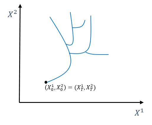
Figure 16: Example of a tree like path.

This notion of tree-like paths is crucial to understand the information that is not captured by the signature as Hambly and Lyons (2010) showed that the signature determines the path up to tree-like equivalence, which we will now define.

Definition 4.3 (Tree-like equivalence).

For $X$ and $Y$ two paths, we say that $X$ and $Y$ are tree-like equivalent if $X*\overleftarrow{Y}$ is a tree-like path. This relation is denoted by $X\sim_{t}Y$.

We can now state Hambly and Lyons’s theorem.

Theorem 4.2.

Let $X\in\mathcal{C}^{1}([0,T],E)$. Then $S(X)=\mathbf{1}$ if and only if $X$ is a tree-like path. Moreover, if $Y\in\mathcal{C}^{1}([0,T],E)$ is another bounded variation path, then $S(X)=S(Y)$ if and only if $X\sim_{t}Y$.

This theorem can be understood as follows: two paths will have the same signature if and only if one can be obtained from the second by using translations, by changing the traversal speeds and by removing parts of the form $W*\overleftarrow{W}$. This uniqueness result has then been extended to a more general class of paths (namely weakly geometric rough paths) by Boedihardjo et al. (2016).

Remark 4.4.

The conclusion of Theorem 4.2 still holds if the signature is replaced by the log-signature since the log mapping is a bijection. Note however that the first statement of the theorem should be modified as follows: $\log(S(X))=\mathbf{0}$ if and only if $X$ is a tree-like path where $\mathbf{0}=(0,\dots,0,\dots)\in T_{0}(E)$.

We have seen that in dimension 1, the signature only captures the path increment between 0 and $T$ (see Example 2.1 in Section 2.2) so that the signature will only allow to distinguish paths $X$ and $Y$ such that $X_{T}-X_{0}\neq Y_{T}-Y_{0}$. This result is actually a consequence of the following proposition and Theorem 4.2.

Proposition 4.5.

If $E$ is a one-dimensional real vector space and $X$, $Y$ are $E$-valued paths such that $X_{T}-X_{0}=Y_{T}-Y_{0}$, then $X$ and $Y$ are tree-like equivalent.

Proof.

Since any one-dimensional real vector space is isometrically isomorph to $\mathbb{R}$, we can assume that $E=\mathbb{R}$. Let $X$ and $Y$ be two paths from $[0,T]$ to $\mathbb{R}$ such that $X_{T}-X_{0}=Y_{T}-Y_{0}$. Let us set $Z=X*\overleftarrow{Y}$ and $h(t)=|Z_{t}-Z_{0}|$ for $t\in[0,2T]$. Using the definition of concatenation operator and the fact that $X_{T}-X_{0}=Y_{T}-Y_{0}$, we have $Z_{0}=X_{0}$ and $Z_{2T}=X_{T}+Y_{0}-Y_{T}=X_{0}$ so that $h(0)=h(2T)=0$. The non-negativity of $h$ results from the non-negativity of the absolute value. Moreover, the continuity of $X$ and $Y$ imply the continuity of $Z$ by definition of the concatenation operator, so $h$ is continuous as well. The only remaining property to show is inequality (4.36). Let $s,t\in[0,2T]$ with $s\leq t$. Let us assume that $Z_{s}\leq Z_{t}$ (the proof in the case $Z_{t}\leq Z_{s}$ is similar) so that $|Z_{t}-Z_{s}|=Z_{t}-Z_{s}=Z_{t}-Z_{0}-(Z_{s}-Z_{0})$. We distinguish three cases:

• If $Z_{0}\leq Z_{s}\leq Z_{t}$, then $h(t)=Z_{t}-Z_{0}$ and $h(s)=Z_{s}-Z_{0}$. Thus,

  $$|Z_{t}-Z_{s}|=h(t)-h(s)\leq h(t)-\inf_{u\in[s,t]}h(u)\leq h(t)+h(s)-2\inf_{u\in[s,t]}h(u).$$ (4.38)

• If $Z_{s}\leq Z_{0}\leq Z_{t}$, then $h(t)=Z_{t}-Z_{0}$ and $h(s)=Z_{0}-Z_{s}$. Thus,

  $$|Z_{t}-Z_{s}|=h(t)+h(s)=h(t)+h(s)-2\inf_{u\in[s,t]}h(u)$$ (4.39)

  because by the intermediate value theorem, there exists $v\in[s,t]$ such that $Z_{v}=Z_{0}$ which implies $\inf_{u\in[s,t]}h(u)=0$.

• If $Z_{s}\leq Z_{t}\leq Z_{0}$, then $h(t)=Z_{0}-Z_{t}$ and $h(s)=Z_{0}-Z_{s}$. Thus,

  $$|Z_{t}-Z_{s}|=h(s)-h(t)\leq h(s)-\inf_{u\in[s,t]}h(u)\leq h(t)+h(s)-2\inf_{u\in[s,t]}h(u).$$ (4.40)

Hence, $h$ is a height function of $Z$ and $Z$ is tree-like. ∎

4.3 Signature and stochastic processes

In the last two subsections, the signature has been presented in a deterministic setting. However, it is clear that the stated results in the previous subsection remain true for stochastic processes by defining the signature as a random variable. In view of the uniqueness theorem from Hambly and Lyons, a natural question at this stage is whether the signature allows to characterize the law of stochastic processes. A first positive answer has been provided by Chevyrev and Lyons (2016). They succeeded to construct a characteristic function for the signature of stochastic processes and they proved that it characterizes the law of stochastic processes in the same way as the traditional characteristic function does for random variables. However, this construction is quite abstract and as such is not suitable for applications so far. They also gave some technical conditions under which the expected signature (defined as $\mathbb{E}[S(X)]$ where $X$ is a stochastic process) characterizes the law.

These results have then been extended by Chevyrev and Oberhauser (2022). They showed that by considering a normalization of the signature, the expected normalized signature characterizes the law of stochastic processes under mild regularity assumptions. This result is stronger than the one from Chevyrev and Lyons as it requires less assumptions. We now provide a brief description of their main result. More details can be found in Appendix D.

Let us denote by $T_{1}^{*}(E)$ the subset of $T^{*}(E)$ (see equation (2.11)) defined by:

$$T^{*}_{1}(E):=\left\{\mathbf{t}\in T^{*}(E)\mid\mathbf{t}^{0}=1\right\}.$$ (4.41)

We define a tensor normalization as follows:

Definition 4.4 (Tensor normalization).

A tensor normalization is a continuous injective map of the form

$$\begin{array}[]{rcl}\Lambda:T_{1}^{*}(E)&\rightarrow&\{\mathbf{t}\in T^{*}_{1}(E)\mid\|\mathbf{t}\|\leq K\}\\ \mathbf{t}&\mapsto&(\mathbf{t}^{0},\lambda(\mathbf{t})\mathbf{t}^{1},\lambda(\mathbf{t})^{2}\mathbf{t}^{2},\dots,\lambda(\mathbf{t})^{n}\mathbf{t}^{n},\dots).\end{array}$$ (4.42)

where $K>0$ is a constant and $\lambda:T^{*}_{1}(E)\rightarrow(0,+\infty)$ is a positive function.

The existence of such object is stated in D.1. We can now state a simplified version of Chevyrev and Oberhauser’s main theorem:

Theorem 4.3.

Let $X=(X_{t})_{t\in[0,T]}$ and $Y=(Y_{t})_{t\in[0,T]}$ be two stochastic processes defined on a probability space $(\Omega,\mathcal{A},\mathbb{P})$ such that $X$ and $Y$ are in $\mathcal{P}^{1}([0,T],E)$ almost surely where $\mathcal{P}^{1}([0,T],E)=\mathcal{C}^{1}([0,T],E)/\sim_{t}$ is the space of bounded variation paths quotiented by the tree-like equivalence relation. Let $\Lambda$ be a tensor normalization and define the normalized signature as $\Phi=\Lambda\circ S$. Then,

$$\mathbb{E}[\Phi(X)]=\mathbb{E}[\Phi(Y)]\text{ iff }X\overset{d}{=}Y.$$ (4.43)

Of course, stochastic processes of interest for financial applications do not have bounded variation. However, as in practice we only consider the values of stochastic processes over a finite grid and we interpolate them linearly, the bounded variation assumption is verified.

Remark 4.5.

The proof of this theorem does not work anymore if we replace the signature by the log-signature. Indeed, one of the key ingredients of the proof is the shuffle product identity (stated below and proved in Theorem 2.15 of Lyons et al., 2007) which holds for the signature but not for the log-signature. If $X:[0,T]\rightarrow E$ with $E$ of dimension $d$, then:

$$\int_{0\leq u_{1}<u_{2}\leq\dots<u_{m}\leq T}dX_{u_{1}}^{i_{1}}\dots dX_{u_{m}}^{i_{m}}\int_{0\leq v_{1}<v_{2}\leq\dots<v_{n}\leq T}dX_{v_{1}}^{i_{1}}\dots dX_{v_{n}}^{i_{n}}$$ (4.44)

$$=\sum_{\sigma\in Shuffles(m,n)}\int_{0\leq w_{1}<w_{2}\dots<w_{m+n}\leq T}dX_{w_{1}}^{k_{\sigma(1)}}\dots dX_{w_{m+n}}^{k_{\sigma(m+n)}}$$

for $(i_{1},\dots,i_{m})\in\{1,\dots,d\}^{m}$, $(j_{1},\dots,j_{n})\in\{1,\dots,d\}^{n}$, $(k_{1},\dots,k_{m+n})=(i_{1},\dots,i_{m},j_{1},\dots,j_{n})$ and

$$Shuffles(m,n)=\left\{\sigma\in\mathfrak{S}_{m+n}\mid\sigma(1)<\dots<\sigma(m)\text{ and }\sigma(m+1)<\dots<\sigma(m+n)\right\}$$ (4.45)

with $\mathfrak{S}_{m+n}$ the permutation group of $\{1,\dots,m+n\}$.

5 Concluding remarks

We propose a new approach for the validation of real-world economic scenarios motivated by insurance applications. This approach relies on the formulation of the problem of validating real-world economic scenarios as a two-sample hypothesis testing problem where the first sample consists of historical paths, the second sample consists of simulated paths of a given real-world stochastic model and the null hypothesis is that the two samples come from the same distribution. For this purpose, we use the statistical test developed by Chevyrev and Oberhauser (2022) which precisely allows to check whether two samples of stochastic processes paths come from the same distribution. It relies on the notions of signature and maximum mean distance which are presented in this article. Our contribution is to study this test from a numerical point of view in settings that are relevant for applications. More specifically, we start by measuring the statistical power of the test on synthetic data under two practical constraints: first, the marginal one-year distributions of the compared samples are equal or very close so that point-in-time validation methods are unable to distinguish the two samples and second, one sample is assumed to be of small size (below 50) while the other is of larger size (1000). To this end, we apply the test to two one-dimensional stochastic processes in continuous time, namely the fractional Brownian motion (fBm) and the Black-Scholes dynamics (BSd) and two time series models, namely a regime-switching $AR(1)$ process and a random walk with i.i.d. Gamma increments. The numerical experiments have highlighted the need to configure the test specifically for each stochastic process to achieve a good statistical power. In particular the truncation order, the path transformation (lead-lag, time lead-lag or cumulative lead-lag), the signature type (signature or log-signature) and the rescaling are key ingredients to be adjusted for each model. For example, the test achieves statistical powers that are close to one in the following settings which illustrate three different risk factors (stock volatility, stock price and inflation respectively):

• fBm paths with Hurst parameter $H=0.1$ against fBm paths with Hurst parameter $H^{\prime}=0.2$ using the lead-lag transformation and the log-signature;

• BSd paths with constant volatility against BSd paths with piecewise constant volatility using the time lead-lag transformation and the log-signature with a proper rescaling or using the cumulative lead-lag transformation along with the signature;

• paths of a regime-switching $AR(1)$ process against paths of a random walk with i.i.d. Gamma increments using the lead-lag transformation along with the log-signature.

In addition to these numerical experiments on synthetic data, we show that the test also performs well on historical data since it rejects some models whereas others are not rejected even if the distributions of the annual log-increments are very close in all the models. For example, we show that the fractional Ornstein-Uhlenbeck model with Hurst parameter around 0.1 is consistent with historical log-volatility of the S&P 500 while the ordinary Ornstein-Uhlenbeck model is not, which is another piece of evidence that volatility is rough (Gatheral et al., 2018). These results indicate that this test represents a promising validation tool for real-world scenarios in a practical framework motivated by insurance applications. More broadly, the test appears as a universal tool for academics and practitioners that would like to challenge a new model against historical data.

Appendix A Sufficient condition for the MMD to be a metric

In this section, we provide a sufficient condition on the Mercer kernel $K$ for the MMD to be a metric. For this purpose, we start by introducing the notions of universality and characteristicness.

Let $\mathcal{X}$ be a topological space and $\mathcal{F}\subset\mathbb{R}^{\mathcal{X}}$ be a topological vector space (TVS). For a TVS $E$, we call any map:

$$\Phi:\mathcal{X}\rightarrow E$$ (A.1)

a feature map for which $E$ is the feature space.

Notation:

we will denote by $E^{\prime}$ the dual of $E$, that is the space of all continuous linear forms on $E$, and by $E^{*}$ the algebraic dual of $E$, that is the space of all linear forms on $E$ (not necessarily continuous).

Definition A.1 (Universality and characteristicness).

Suppose that $\langle l,\Phi(\cdot)\rangle\in\mathcal{F}$ for all $l\in E^{\prime}$. We say that $\Phi$ is

• universal to $\mathcal{F}$ if the map

  $$\begin{array}[]{rrcl}\iota:&E^{\prime}&\rightarrow&\mathbb{R}^{\mathcal{X}}\\ &l&\mapsto&\langle l,\Phi(\cdot)\rangle\end{array}$$ (A.2)

  has a dense image in $\mathcal{F}$, i.e. $\overline{\iota(E^{\prime})}=\mathcal{F}$.

• characteristic to a subset $\mathcal{P}\subset\mathcal{F}^{\prime}$ if the map

  $$\begin{array}[]{rrcl}\kappa:&\mathcal{P}&\rightarrow&(E^{\prime})^{*}\\ &D&\mapsto&\left[l\mapsto D(\langle l,\Phi(\cdot)\rangle)\right]\end{array}$$ (A.3)

  is one-to-one.

These two notions are actually equivalent under mild assumptions. We refer to Trèves (1967) for a definition of a locally convex topological vector space.

Theorem A.1.

Suppose that $\mathcal{F}$ is a locally convex TVS. Then, a feature map $\Phi$ is universal to $\mathcal{F}$ iff $\Phi$ is characteristic to $\mathcal{F}^{\prime}$.

Proof.

Let us first assume that $\Phi$ is universal to $\mathcal{F}$. Let $D_{1},D_{2}\in\mathcal{F}^{\prime}$ such that $\kappa(D_{1})=\kappa(D_{2})$. Then, for all $l\in E^{\prime}$, we have $\kappa(D_{1})(l)=\kappa(D_{2})(l)$, that is $D_{1}(\langle l,\Phi(\cdot)\rangle)=D_{2}(\langle l,\Phi(\cdot)\rangle)$, which rewrites $D_{1}(\iota(l))=D_{2}(\iota(l))$. Therefore, $D_{1}$ and $D_{2}$ coincide on $\iota(E^{\prime})$. Since $\iota(E^{\prime})$ is dense in $\mathcal{F}$ by hypothesis and $D_{1}$ and $D_{2}$ are continuous, we have $D_{1}=D_{2}$ on $\mathcal{F}$. Hence, $\kappa$ is one-to-one and $\Phi$ is characteristic to $\mathcal{F}^{\prime}$.
Now assume that $\Phi$ is not universal to $\mathcal{F}$, i.e. $\iota(E^{\prime})$ is not dense in $\mathcal{F}$. By assumption, we have $\iota(E^{\prime})\subset\mathcal{F}$, $\overline{\iota(E^{\prime})}\neq\mathcal{F}$ and $\mathcal{F}$ is a locally convex TVS. According to a corollary of the Hahn-Banach theorem (see corollary 3 of theorem 18.1 in Trèves, 1967), there exists under these assumptions $f\in\mathcal{F}^{\prime}$ such that $f\neq 0$ but $f|_{\iota(E^{\prime})}=0$. As a consequence, $\kappa(f)(l)=f(\iota(l))=0$ for all $l\in E^{\prime}$, so we have $\kappa(f)=\kappa(0)$ but $f\neq 0$. Hence, $\kappa$ is not one-to-one and $\Phi$ is not characteristic to $\mathcal{F}^{\prime}$. ∎

These notions of universality and characteristicness can also be defined for Mercer kernels.

Definition A.2.

Let $K$ be a Mercer kernel and denote by $\mathcal{H}$ the associated RKHS. Let $\mathcal{F}\subset\mathbb{R}^{\mathcal{X}}$ be a TVS such that $\mathcal{H}\subset\mathcal{F}$. We say that $K$ is:

• universal to $\mathcal{F}$ if the RKHS $\mathcal{H}$ of $K$ is dense in $\mathcal{F}$

• characteristic to $\mathcal{F}^{\prime}$ if the map:

  $$\begin{array}[]{rrcl}\kappa:&\mathcal{F}^{\prime}&\rightarrow&\mathcal{H}^{\prime}\\ &D&\mapsto&D_{|\mathcal{H}}\end{array}$$ (A.4)

  is one-to-one.

We have a similar theorem to Theorem A.1 (the proof is similar as well).

Theorem A.2.

Suppose that $\mathcal{F}$ is a locally convex TVS. Then a kernel $K$ is universal to $\mathcal{F}$ iff $K$ is characteristic to $\mathcal{F}^{\prime}$.

The link between the universality/characteristicness of a feature map $\Psi$ and the universality/characteristicness of the associated kernel $K(x,y):=\langle\Psi(x),\Psi(y)\rangle$ is stated in the following lemma due to Chevyrev and Oberhauser (2022).

Lemma A.1.

Consider a map $\Psi:\mathcal{X}\rightarrow E$ where $E$ is equipped with a scalar product $\langle\cdot,\cdot\rangle$ and define $K(x,y)=\langle\Psi(x),\Psi(y)\rangle$. If $\mathcal{F}$ is a locally convex TVS such that $\mathcal{H}_{0}:=\operatorname{span}\left\{K_{x}:=K(x,\cdot)\mid x\in\mathcal{X}\right\}$ continuously embeds into $\mathcal{F}$, then $\Psi$ is universal to $\mathcal{F}$ iff $K$ is universal to $\mathcal{F}$.

We state now a sufficient condition on the kernel $K$ for the MMD to be a metric.

Theorem A.3.

Let $K$ be a Mercer kernel and $\mathcal{F}$ be the space of bounded continuous functions on $\mathcal{X}$. If $K$ is universal to $\mathcal{F}$ and $\mathcal{G}$ is the unit ball of the RKHS $\mathcal{H}$ associated to $K$, then $MMD_{\mathcal{G}}$ is a metric on the space $\mathcal{M}$ defined as:

$$\mathcal{M}=\left\{\mu\text{ Borel probability measure defined on }\mathcal{X}\middle|\int_{\mathcal{X}}\sqrt{K(x,x)}\mu(dx)<\infty\right\}.$$ (A.5)

Proof.

Since the MMD is a pseudo-metric, we only have to prove that $MMD_{\mathcal{G}}(\mu,\nu)=0$ implies $\mu=\nu$. Assume that $MMD_{\mathcal{G}}(\mu,\nu)=0$. According to Lemma B.2 in Appendix B, we therefore have $\|\varphi_{\mu}-\varphi_{\nu}\|_{\mathcal{H}}=0$, i.e. $\varphi_{\mu}=\varphi_{\nu}$. As a consequence, we have for all $f\in\mathcal{H}$:

$$\int_{\mathcal{X}}f(x)\mu(dx)=\langle f,\varphi_{\mu}\rangle_{\mathcal{H}}=\langle f,\varphi_{\nu}\rangle_{\mathcal{H}}=\int_{\mathcal{X}}f(x)\nu(dx).$$ (A.6)

Thus, $\mu$ and $\nu$ (seen as linear forms) are equal on $\mathcal{H}$. Since $K$ is universal to $\mathcal{F}$, it is characteristic to $\mathcal{F}^{\prime}$ which is the space of finite regular Borel measures on $\mathcal{X}$ (see Giles, 1971 for a proof). The definition of characteristicness allows to conclude that $\mu=\nu$. ∎

Remark A.1.

Since universality is equivalent to characteristicness, the previous theorem can be stated using one or the other assumption. We prefer the assumption of universality as it is easier to prove in practice.

Appendix B Proof of Theorem 2.2

As a preliminary to the proof, we give some definitions and lemmas.

Definition B.1 (Mean embedding).

Let $\mathcal{H}\subset\mathbb{R}^{\mathcal{X}}$ be a RKHS and $\mu$ be a probability measure on $\mathcal{X}$. When it exists, the mean embedding of $\mu$ is defined as the element $\varphi_{\mu}\in\mathcal{H}$ satisfying $\int_{\mathcal{X}}f(x)\mu(dx)=\langle f,\varphi_{\mu}\rangle_{\mathcal{H}}$ for all $f\in\mathcal{H}$.

The mean embedding doesn’t always exist. The following lemma ensures that under the assumptions of Theorem 2.2 the mean embedding exists.

Lemma B.1.

If $\int_{\mathcal{X}}\sqrt{K(x,x)}\mu(dx)<\infty$, then the mean embedding of $\mu$ exists and we have:

$$\varphi_{\mu}(x)=\int_{\mathcal{X}}K(x,y)\mu(dy).$$ (B.1)

Proof.

The idea is simply to apply Riesz representation theorem. We define the linear form $T_{\mu}$ on $\mathcal{H}$ as $T_{\mu}(f)=\int_{\mathcal{X}}f(x)\mu(dx)$ for all $f\in\mathcal{H}$ and we show that is is continuous. Let $f\in\mathcal{H}$, then $f$ is integrable with respect to $\mu$ since for all $x\in\mathcal{X}$,

$$|f(x)|=|\langle f,K_{x}\rangle_{\mathcal{H}}|\leq\|f\|_{\mathcal{H}}\|K_{x}\|_{\mathcal{H}}=\|f\|_{\mathcal{H}}\sqrt{\langle K_{x},K_{x}\rangle_{\mathcal{H}}}=\|f\|_{\mathcal{H}}\sqrt{K(x,x)}$$ (B.2)

where the first and last equalities are obtained using the reproducing property. By hypothesis $\sqrt{K(x,x)}$ is integrable with respect to $\mu$, so

$$|T_{\mu}(f)|\leq\int_{\mathcal{X}}|f(x)|\mu(dx)\leq\|f\|_{\mathcal{H}}\int_{\mathcal{X}}\sqrt{K(x,x)}\mu(dx).$$ (B.3)

Thus, $T_{\mu}$ is continuous and by Riesz representation theorem, there exists $\varphi_{\mu}\in\mathcal{H}$ such that $T_{\mu}(f)=\langle f,\varphi_{\mu}\rangle_{\mathcal{H}}$ for all $f\in\mathcal{H}$. In particular, we have for all $x\in\mathcal{X}$:

$$\varphi_{\mu}(x)=\langle\varphi_{\mu},K_{x}\rangle_{\mathcal{H}}=T_{\mu}(K_{x})=\int_{\mathcal{X}}K(x,y)\mu(dy).$$ (B.4)

∎

The mean embedding allows to rewrite the MMD in a very simple form when $\mathcal{G}$ is the unit ball in a reproducing kernel Hilbert space.

Lemma B.2.

Under the assumptions of Lemma B.1, for two probability measures $\mu$ and $\nu$, we have:

$$MMD^{2}_{\mathcal{G}}(\mu,\nu)=\|\varphi_{\mu}-\varphi_{\nu}\|_{\mathcal{H}}^{2}$$ (B.5)

when $\mathcal{G}=\{f\in\mathcal{H}\mid\|f\|_{\mathcal{H}}\leq 1\}$

Proof.

$$MMD^{2}_{\mathcal{G}}(\mu,\nu) =\left[\sup_{\|f\|_{\mathcal{H}}\leq 1}\left|\int_{\mathcal{X}}f(x)\mu(dx)-\int_{\mathcal{X}}f(x)\nu(dx)\right|\right]^{2}$$ (B.6)

$$=\left[\sup_{\|f\|_{\mathcal{H}}\leq 1}\left|\langle\varphi_{\mu}-\varphi_{\nu},f\rangle_{\mathcal{H}}\right|\right]^{2}$$

$$=\|\varphi_{\mu}-\varphi_{\nu}\|_{\mathcal{H}}^{2}.$$

∎

The proof of Theorem 2.2 is now straightforward:

Proof of Theorem 2.2.

According to Lemma B.2, we have:

$$MMD^{2}_{\mathcal{G}}(\mu,\nu) =\|\varphi_{\mu}-\varphi_{\nu}\|_{\mathcal{H}}^{2}$$ (B.7)

$$=\langle\varphi_{\mu},\varphi_{\mu}\rangle_{\mathcal{H}}+\langle\varphi_{\nu},\varphi_{\nu}\rangle_{\mathcal{H}}-2\langle\varphi_{\mu},\varphi_{\nu}\rangle_{\mathcal{H}}$$

$$=\int_{\mathcal{X}}\varphi_{\mu}(x)\mu(dx)+\int_{\mathcal{X}}\varphi_{\nu}(x)\nu(dx)-2\int_{\mathcal{X}}\varphi_{\nu}(x)\mu(dx)$$

$$=\int_{\mathcal{X}\times\mathcal{X}}K(x,y)\mu(dx)\mu(dy)+\int_{\mathcal{X}\times\mathcal{X}}K(x,y)\nu(dx)\nu(dy)-2\int_{\mathcal{X}\times\mathcal{X}}K(x,y)\mu(dx)\nu(dy),$$

where the third equality comes from the definition of the mean embeddings and the fourth equality comes from Lemma B.1. ∎

Appendix C Proof of Theorem 2.3

We start by proving the continuity of the signature map. For this purpose, we first introduce the definition of the total variation norm.

Definition C.1 (Total variation norm).

Let $E$ be a vector space endowed with a norm $\|\cdot\|_{E}$. The total variation norm on the set $\mathcal{C}^{1}([0,T],E)$ of bounded variation paths is defined as:

$$\|X\|_{\mathcal{C}^{1}([0,T],E)}=\|X\|_{1,[0,T]}+\sup_{t\in[0,T]}\|X_{t}\|_{E}$$ (C.1)

where we recall that $\|\cdot\|_{1,[0,T]}$ is the total variation (see Definition 2.3).

Lemma C.1.

The signature map defined on bounded variation paths:

$$\begin{array}[]{rcl}S:\left(\mathcal{C}^{1}([0,T],E),\|\cdot\|_{\mathcal{C}^{1}([0,T],E)}\right)&\rightarrow&\left(T_{1}^{*}(E),\|\cdot\|\right)\\ X&\mapsto&S(X)\end{array}$$ (C.2)

is continuous (we recall that $\|\cdot\|$ is the norm defined in equation (2.11)).

Proof.

Consider a sequence of bounded variation paths $(X_{n})_{n\geq 0}$ converging to some $X\in\mathcal{C}^{1}([0,T],E)$ in total variation norm. We have:

$$\|S(X_{n})-S(X)\| =\sum_{k\geq 0}\|\mathbf{X}_{n}^{k}-\mathbf{X}^{k}\|_{E^{\otimes k}}$$ (C.3)

$$=\sum_{k=0}^{N}\|\mathbf{X}_{n}^{k}-\mathbf{X}^{k}\|_{E^{\otimes k}}+\sum_{k\geq N+1}\|\mathbf{X}_{n}^{k}-\mathbf{X}^{k}\|_{E^{\otimes k}}$$

for some $N\geq 0$. First, note that we have:

$$\|\mathbf{X}_{n}^{k}-\mathbf{X}^{k}\|_{E^{\otimes k}} \leq\|\mathbf{X}_{n}^{k}\|_{E^{\otimes k}}+\|\mathbf{X}^{k}\|_{E^{\otimes k}}$$ (C.4)

$$\leq\frac{1}{k!}\left(\|X_{n}\|^{k}_{1,[0,T]}+\|X\|^{k}_{1,[0,T]}\right)$$

$$\leq\frac{1}{k!}\left(\|X_{n}\|^{k}_{\mathcal{C}^{1}([0,T],E)}+\|X\|^{k}_{\mathcal{C}^{1}([0,T],E)}\right)$$

$$\leq\frac{1}{k!}\left(\|X_{n}\|^{k}_{\mathcal{C}^{1}([0,T],E)}+\|X\|^{k}_{\mathcal{C}^{1}([0,T],E)}\right)$$

$$\leq\frac{1}{k!}\left(M^{k}+\|X\|^{k}_{\mathcal{C}^{1}([0,T],E)}\right)$$

where the second inequality results from Proposition 2.2 in Lyons et al. (2007) and $M=\sup_{n\geq 0}\|X_{n}\|_{\mathcal{C}^{1}([0,T],E)}$ which is finite since $(X_{n})_{n\geq 0}$ is convergent in total variation norm. We deduce that $\sup_{n\geq 0}\sum_{k\geq N+1}\|\mathbf{X}_{n}^{k}-\mathbf{X}^{k}\|_{E^{\otimes k}}\underset{N\to+\infty}{\rightarrow}0$. Moreover, we have:

$$\sum_{k=0}^{N}\|\mathbf{X}_{n}^{k}-\mathbf{X}^{k}\|_{E^{\otimes k}} =\|S^{N}_{[0,T]}(X_{n})-S^{N}_{[0,T]}(X)\|$$ (C.5)

$$\leq\sup_{t\in[0,T]}\|S^{N}_{[0,t]}(X_{n})-S^{N}_{[0,t]}(X)\|$$

$$\leq\|S^{N}_{[0,\cdot]}(X_{n})-S^{N}_{[0,\cdot]}(X)\|_{\mathcal{C}^{1}([0,T],T^{N}(E))}.$$

According to Corollary 2.11 in Lyons et al. (2007), the truncated signature

$$\begin{array}[]{rcl}S^{N}_{[0,\cdot]}:\mathcal{C}^{1}([0,T],E)&\rightarrow&\mathcal{C}^{1}([0,T],T^{N}(E))\\ X&\mapsto&t\mapsto S^{N}_{[0,t]}(X)\end{array}$$ (C.6)

where $T^{N}(E)$ is the space of truncated formal series of tensors of order $N$, is continuous in total variation norm. Thus, $\sum_{k=0}^{N}\|\mathbf{X}_{n}^{k}-\mathbf{X}^{k}\|_{E^{\otimes k}}\underset{n\to+\infty}{\rightarrow}0$. Hence $\|S(X_{n})-S(X)\|\underset{n\to+\infty}{\rightarrow}0$. ∎

We can now prove Theorem 2.3.

Proof of Theorem 2.3.

We start by showing that $K^{sig}$ is a Mercer kernel. The symmetry of $K^{sig}$ is deduced from the symmetry of $\langle\cdot,\cdot\rangle$. The continuity arises from the continuity of the signature (Lemma C.1), which is preserved by the tensor normalization, and of $\langle\cdot,\cdot\rangle$. Finally, for $\alpha_{1},\dots,\alpha_{n}\in\mathbb{R}$ and $x_{1},\dots,x_{n}\in\mathcal{P}^{1}([0,T],E)$, we have:

$$\sum_{i=1}^{n}\sum_{j=1}^{n}\alpha_{i}\alpha_{j}K^{sig}(x_{i},x_{j})=\sum_{i=1}^{n}\sum_{j=1}^{n}\alpha_{i}\alpha_{j}\left\langle\Phi(x_{i}),\Phi(x_{j})\right\rangle=\left\|\sum_{i=1}^{n}\alpha_{i}\Phi(x_{i})\right\|^{2}\geq 0.$$ (C.7)

Thus, $K^{sig}$ is also positive semi-definite and thereby $K^{sig}$ is a Mercer kernel. As such, Moore-Aronszajn’s theorem can be applied and we can associate a RKHS $\mathcal{H}^{sig}$ to the kernel $K^{sig}$. A direct application of Theorem 2.2 yields equation (2.16).
The only remaining point to show is that $MMD_{\mathcal{G}}$ is a metric. Let $\mathcal{F}$ be the space of bounded continuous functions on $\mathcal{P}^{1}([0,T],E)$. According to Theorem D.1 in Appendix D.2, $\Phi$ is universal to $\mathcal{F}$. Next, we show that $\mathcal{H}_{0}:=\operatorname{span}\left\{K^{sig}_{x}:=K^{sig}(x,\cdot)\mid x\in\mathcal{P}^{1}([0,T],E)\right\}$ continuously embeds into $\mathcal{F}$. Let us equip $\mathcal{H}_{0}$ with the scalar product $\langle\cdot,\cdot\rangle_{\mathcal{H}_{0}}$ defined by:

$$\langle f,g\rangle_{\mathcal{H}_{0}}:=\sum_{i=1}^{r}\sum_{j=1}^{s}\alpha_{i}\beta_{j}K^{sig}(x_{i},y_{j})\quad\text{for }f=\sum_{i=1}^{r}\alpha_{i}K^{sig}_{x_{i}}\text{ and }g=\sum_{i=1}^{s}\beta_{i}K^{sig}_{y_{i}}.$$ (C.8)

It is clear that $\mathcal{H}_{0}$ satisfies the reproducing property. Therefore, if $f\in\mathcal{H}_{0}$, then for all $x\in\mathcal{P}^{1}([0,T],E)$,

$$f(x)=\langle f,K_{x}^{sig}\rangle_{\mathcal{H}_{0}}\leq\|f\|_{\mathcal{H}_{0}}\|K_{x}^{sig}\|_{\mathcal{H}_{0}}$$ (C.9)

using the Cauchy-Schwarz inequality. By definition of $\|\cdot\|_{\mathcal{H}_{0}}$, we have

$$\|K_{x}^{sig}\|_{\mathcal{H}_{0}}=\sqrt{K^{sig}(x,x)}=\sqrt{\langle\Phi(x),\Phi(x)\rangle_{T(E)}}=\|\Phi(x)\|_{T(E)}\leq K$$ (C.10)

where the last inequality comes from the definition of the tensor normalization. We deduce that:

$$\|f\|_{\infty}=\sup_{x\in\mathcal{X}}|f(x)|\leq K\|f\|_{\mathcal{H}_{0}}$$ (C.11)

i.e. $\mathcal{H}_{0}$ continuously embeds into $\mathcal{F}$ endowed with the uniform norm $\|\cdot\|_{\infty}$. Thus, according to Lemma A.1, $K^{sig}$ is universal to $\mathcal{F}$. Finally, using Theorem A.3, we conclude that $MMD_{\mathcal{G}}$ is a metric. ∎

Remark C.1.

A natural question is whether Theorem 2.3 can be extended to $K^{sig}(x,y)=K(\Phi(x),\Phi(y))$ where $K$ is a Mercer kernel on $T(E)\times T(E)$. It is easy to show that in this case, $K^{sig}$ is still a Mercer kernel. However, we don’t know if the conclusion of Lemma A.1 still holds with this definition.

Appendix D Characterization of stochastic processes law by the expected normalized signature

D.1 Normalization existence

In this subsection, we discuss the existence of tensor normalizations. The following proposition is proved in Proposition 14 of Chevyrev and Oberhauser (2022).

Proposition D.1.

Let $\psi:[1,+\infty)\rightarrow[1,+\infty)$ with $\psi(1)=1$. For $\mathbf{t}\in T^{*}_{1}(E)$, let $\lambda(\mathbf{t})\geq 0$ denote the unique $\lambda$ such that:

$$\sum_{n\geq 0}\lambda^{2n}\|\mathbf{t}^{n}\|^{2}_{E^{\otimes n}}=\psi(\|\mathbf{t}\|)$$ (D.1)

and define $\Lambda$ as in Definition 4.4 with $\lambda(\mathbf{t})$ as specified above. Denote further $\|\psi\|_{\infty}=\sup_{x\geq 1}\psi(x)$. Under the following assumptions on $\psi$:

1. $\psi$ is one-to-one,

2. $\|\psi\|_{\infty}<\infty$,

3. $\sup_{x\geq 1}\frac{\psi(x)}{x^{2}}\leq 1$,

4. $\psi$ is $K$-Lipschitz for some $K>0$,

then $\Lambda$ is a tensor normalization.

Remark D.1.

Although it is not discussed by Chevyrev and Oberhauser, a solution to equation (D.1) a priori doesn’t always exist. Indeed, the left-hand term can be seen as a power series in $\lambda$ (with only even terms):

$$P(\lambda)=\sum_{n\geq 0}\lambda^{2n}\|\mathbf{t}^{n}\|^{2}_{E^{\otimes n}}.$$ (D.2)

Its radius of convergence is greater or equal to 1 since by definition of $T^{*}(E)$, we have $\|\mathbf{t}\|<\infty$. Thus, on $[0,1]$, $P$ is continuous and strictly increasing with $P(0)=1$ and $P(1)=\|\mathbf{t}\|$. As such, if $\psi(\|t\|)$ is greater than $\|\mathbf{t}\|$, there is a priori no reason for the existence of a solution to (D.1) without further assumption on the rate of decay of the sequence $(\|\mathbf{t}^{n}\|_{E^{\otimes n}})_{n\geq 0}$. However, if we choose $\mathbf{t}$ as the signature of some path $X$, we know that (see Lyons et al., 2007) $\|\mathbf{t}^{n}\|_{E^{\otimes n}}$ decays as $\frac{\|X\|_{1,[0,T]}^{n}}{n!}$ if $X$ is of bounded variation. As a consequence, if $\mathbf{t}$ is the signature of some path with bounded variation, the radius of convergence of $P$ is infinite and equation (D.1) indeed has a unique solution. Anyway, in practice the power series is truncated and there is always a unique solution belonging to $\mathbb{R}_{+}$.

In their numerical experiments, Chevyrev and Oberhauser consider the following form for $\psi$:

$$\psi(x)=\left\{\begin{array}[]{ll}x^{2}&\text{if }x\leq\sqrt{M}\\ M+M^{1+a}(M^{-a}-x^{-2a})/a&\text{if }x>\sqrt{M}\end{array}\right.$$ (D.3)

with $M=4$ and $a=1$. This function clearly satisfies the hypotheses of Proposition D.1 so $\Lambda$ constructed from $\psi$ is a tensor normalization.

D.2 General version of Theorem 4.3

In this section, we present a more general version of Theorem 4.3.

We recall that $\mathcal{C}^{1}([0,T],E)$ is the set of bounded variation paths from $[0,T]$ to $E$ and $\mathcal{P}^{1}([0,T],E)$ is the set of bounded variation paths quotiented by the tree-like equivalence relation. As there is no ambiguity here, we juste write $\mathcal{C}^{1}$ and $\mathcal{P}^{1}$. We denote by $C_{b}(\mathcal{P}^{1},\mathbb{R})$ the space of continuous bounded functions from $\mathcal{P}^{1}$ to $\mathbb{R}$. This space can be equipped with the strict topology which is for example defined by Giles (1971). With these notations, we have the following theorem due to Chevyrev and Oberhauser (Theorem 21 in Chevyrev and Oberhauser, 2022).

Theorem D.1.

Let $\Lambda$ be a tensor normalization. Then the map

$$\begin{array}[]{rcl}\Phi:\mathcal{P}^{1}&\rightarrow&T^{*}_{1}(E)\\ X&\mapsto&\Lambda\circ S(X)\end{array}$$ (D.4)

1. is a continuous injection from $\mathcal{P}^{1}$ into a bounded subset of $T^{*}_{1}(E)$,

2. is universal to $\mathcal{F}:=C_{b}(\mathcal{P}^{1},\mathbb{R})$ equipped with the strict topology,

3. is characteristic to the space of finite regular Borel measures on $\mathcal{P}^{1}$.

The same statement holds when $\mathcal{P}^{1}$ is replaced by $\mathcal{C}^{1}$ and $\Phi$ is replaced by $\bar{\Phi}:=\Lambda\circ S(\bar{X})$ where $\bar{X}(t)=(X(t),t)$.

Remark D.2.

Theorem 4.3 follows from (iii) and Lemma D.1.

The following lemma combined with Theorem A.1 shows that Theorem 4.3 is a consequence of the theorem above.

Lemma D.1.

Under the assumptions:

1. $(E,\langle\cdot,\cdot\rangle_{E})$ is a Hilbert space,

2. $\mathcal{F}^{\prime}$ consists of finite measures on $\mathcal{X}$,

3. $\|\Phi\|_{\infty}=\sup_{x\in\mathcal{X}}\|\Phi(x)\|_{E}<\infty$,

then the characteristicness of the feature map $\Phi$ (i.e. the injectivity of $\kappa$ defined in (A.3)) implies the injectivity of the mapping $\tilde{\kappa}$ defined as:

$$\begin{array}[]{rrcl}\tilde{\kappa}:&\mathcal{F}^{\prime}&\rightarrow&E\\ &\mu&\mapsto&\int_{\mathcal{X}}\Phi(x)\mu(dx)\end{array}$$ (D.5)

Proof.

Let $\mu_{1}$ and $\mu_{2}$ in $\mathcal{F}^{\prime}$ such that $\tilde{\kappa}(\mu_{1})=\tilde{\kappa}(\mu_{2})$. This can be rewritted:

$$\int_{\mathcal{X}}\Phi(x)\mu_{1}(dx)=\int_{\mathcal{X}}\Phi(x)\mu_{2}(dx).$$ (D.6)

Let $l\in E^{\prime}$, we have:

$$\left\langle l,\int_{\mathcal{X}}\Phi(x)\mu_{1}(dx)\right\rangle=\left\langle l,\int_{\mathcal{X}}\Phi(x)\mu_{2}(dx)\right\rangle$$ (D.7)

Identifying $l$ with its Riesz representation, we have:

$$|\langle l,\Phi(x)\rangle_{E}|\leq\|l\|_{E}\|\Phi(x)\|_{E}\leq\|l\|_{E}\|\Phi\|_{\infty}$$ (D.8)

Since $\mu_{1}$ is a finite measure, we deduce that $\int_{\mathcal{X}}\left|\langle l,\Phi(x)\rangle_{E}\right|\mu_{1}(dx)<\infty$. Thus, we can interchange the integral and the scalar product, which yields:

$$\int_{\mathcal{X}}\langle l,\Phi(x)\rangle\mu_{1}(dx)=\int_{\mathcal{X}}\langle l,\Phi(x)\rangle\mu_{2}(dx),$$ (D.9)

which is exactly $\kappa(\mu_{1})(l)=\kappa(\mu_{2})(l)$. Thus $\mu_{1}=\mu_{2}$ by injectivity of $\kappa$. ∎

Appendix E Zero odd-order restricted MMD between centered Gaussian processes

In this section, we justify theoretically why the MMD restricted to odd orders doesn’t allow to distinguish fBm’s with different Hurst parameters. We first need the following lemma.

Lemma E.1.

Let $X$ be a real-valued stochastic process. We consider a partition $0=t_{0}<t_{1/2}<t_{1}<\dots<t_{N-1/2}<t_{N}=T$ of $[0,T]$ and we denote by $\hat{X}$ the lead-lag transformation of $X$ on this partition. Then, for all $k\in\mathbb{N}$, for all $I=(i_{1},\dots,i_{k})\in\{1,2\}^{k}$ (with the convention $I=1$ if $k=0$) and for all $s\in[0,T]$, we have:

$$\mathbf{\hat{X}}^{k}_{I,[0,s]}=\sum_{\alpha\in\mathcal{J}_{k}(\tau(s)+1)}P_{\alpha,\tau(s)}(s)X_{t_{0}}^{\alpha_{0}}X_{t_{1}}^{\alpha_{1}}\dots X_{t_{\tau(s)+1}}^{\alpha_{\tau(s)+1}}$$ (E.1)

where

• $\mathbf{\hat{X}}^{k}_{I,[0,s]}$ is the coefficient at position $I$ of the $k$-th term of the signature of $\hat{X}$ on $[0,s]$

• $\tau(s)\in\{0,\dots,N-1\}$ is such that $t_{\tau(s)}\leq s<t_{\tau(s)+1}$

• $\mathcal{J}_{k}(l)=\left\{\alpha=(\alpha_{0},\dots,\alpha_{l})\in\{0,\dots,k\}^{l}\mid\sum_{i=0}^{l}\alpha_{i}=k\right\}$

• $P_{\alpha,i}(s)$ is a polynomial in $s$ that depends on $\alpha$ and $t_{0},t_{1/2},\dots,t_{i+1/2},t_{i+1}$ but not on $X$.

Proof.

We proceed by induction on $k$. If $k=0$, then by definition of the signature, $\mathbf{\hat{X}}^{0}_{1,[0,s]}=1$ for all $s\in[0,T]$ so (E.1) is verified. Let us assume that (E.1) is verified for some $k\geq 0$. Let $I=(i_{1},\dots,i_{k+1})\in\{1,2\}^{k+1}$ and $s\in[0,T]$. We set $I^{\prime}=(i_{1},\dots,i_{k})$. By definition of the signature, we have:

$$\begin{array}[]{rl}\mathbf{\hat{X}}^{k+1}_{I,[0,s]}&=\displaystyle\int_{0<u_{1}<\dots<u_{k+1}<s}d\hat{X}_{u_{1}}^{i_{1}}\times\dots\times d\hat{X}_{u_{k+1}}^{i_{k+1}}\\ &=\displaystyle\int_{0}^{s}\mathbf{\hat{X}}^{k}_{I^{\prime},[0,u]}d\hat{X}^{i_{k}+1}_{u}\\ &=\displaystyle\sum_{i=0}^{\tau(s)-1}\int_{t_{i}}^{t_{i+1}}\mathbf{\hat{X}}^{k}_{I^{\prime},[0,u]}d\hat{X}^{i_{k}+1}_{u}+\int_{\tau(s)}^{s}\mathbf{\hat{X}}^{k}_{I^{\prime},[0,u]}d\hat{X}^{i_{k}+1}_{u}\\ &=\displaystyle\sum_{i=0}^{\tau(s)-1}\int_{t_{i}}^{t_{i+1}}\left(\sum_{\alpha\in\mathcal{J}_{k}(\tau(u)+1)}P_{\alpha,\tau(u)}(u)X_{t_{0}}^{\alpha_{0}}\dots X_{\tau(u)+1}^{\alpha_{\tau(u)+1}}\right)d\hat{X}^{i_{k}+1}_{u}\\ &+\displaystyle\int_{\tau(s)}^{s}\left(\sum_{\alpha\in\mathcal{J}_{k}(\tau(u)+1)}P_{\alpha,\tau(s)}(u)X_{t_{0}}^{\alpha_{0}}\dots X_{\tau(s)+1}^{\alpha_{\tau(s)+1}}\right)d\hat{X}^{i_{k}+1}_{u}\\ &=\displaystyle\sum_{i=0}^{\tau(s)-1}\sum_{\alpha\in\mathcal{J}_{k}(i+1)}X_{t_{0}}^{\alpha_{0}}\dots X_{t_{i+1}}^{\alpha_{i+1}}\int_{t_{i}}^{t_{i+1}}P_{\alpha,\tau(u)}(u)d\hat{X}^{i_{k}+1}_{u}\\ &+\displaystyle\sum_{\alpha\in\mathcal{J}_{k}(\tau(s)+1)}X_{t_{0}}^{\alpha_{0}}\dots X_{\tau(s)+1}^{\alpha_{\tau(s)+1}}\displaystyle\int_{\tau(s)}^{s}P_{\alpha,\tau(s)}(u)d\hat{X}^{i_{k}+1}_{u}\end{array}$$ (E.2)

Using the definition of the lead-lag transformation, it is easy to see that if $i_{k+1}=1$ (corresponding to the lead component) and $u\in[t_{i},t_{i+1}]$:

$$d\hat{X}_{u}^{i_{k+1}}=\frac{X_{t_{i+1}}-X_{t_{i}}}{t_{i+1/2}-t_{i}}\mathbb{1}_{[t_{i},t_{i+1/2}]}(u)du$$ (E.3)

with the notations introduced in subsection 3.1.2. Similarly, if $i_{k+1}=2$ (corresponding to the lag component) and $u\in[t_{i},t_{i+1}]$:

$$d\hat{X}_{u}^{i_{k+1}}=\frac{X_{t_{i+1}}-X_{t_{i}}}{t_{i+1}-t_{i+1/2}}\mathbb{1}_{[t_{i+1/2},t_{i+1}]}(u)du.$$ (E.4)

Since the integral of a polynomial is still a polynomial and for $i\in\{0,\dots,\tau(s)-1\}$, $\mathcal{J}_{k}(i+1)$ can be seen as a subset of $\mathcal{J}_{k}(\tau(s)+1)$ by adding zero entries at the end, we finally get

$$\mathbf{\hat{X}}^{k+1}_{I,[0,s]}=\sum_{\alpha\in\mathcal{J}_{k+1}(\tau(s)+1)}\tilde{P}_{\alpha,\tau(s)}(s)X_{t_{0}}^{\alpha_{0}}X_{t_{1}}^{\alpha_{1}}\dots X_{t_{\tau(s)+1}}^{\alpha_{\tau(s)+1}}.$$ (E.5)

On the one hand, the integration of each term of the sum in equation (E.1) on $[0,\tau(s)]$ does not increase the degree of the polynomial in $s$ and yields two polynomials in $X_{t_{0}},\dots,X_{t_{\tau(s)}}$ whose sum of degrees (given by the $\alpha_{i}$’s) equals $k+1$ because of the multiplication by the increment $X_{t_{i+1}}-X_{t_{i}}$ on $[t_{i},t_{i+1}]$ with $i\leq\tau(s)-1$. On the other hand, the integration on $[\tau(s),s]$ increases by one the degree of the polynomial in $s$ and yields two polynomials in $X_{t_{0}},\dots,X_{t_{\tau(s)+1}}$ whose sum of degrees also equals $k+1$. ∎

We recall that the signature kernel is defined by $K^{sig}(X,Y)=\langle S(X),S(Y)\rangle$ where $\langle\cdot,\cdot\rangle$ is the scalar product on $T^{*}(E)$ defined by:

$$\langle\mathbf{x},\mathbf{y}\rangle=\sum_{n\geq 0}\langle\mathbf{x}^{n},\mathbf{y}^{n}\rangle_{E^{\otimes n}}$$ (E.6)

for $\mathbf{x}$ and $\mathbf{y}$ in $T^{*}(E)$. We now define the signature kernel restricted at order $l$ as:

$$K^{sig}_{\ell}(X,Y)=\langle\mathbf{X}^{\ell},\mathbf{Y}^{\ell}\rangle_{E^{\otimes\ell}}$$ (E.7)

as well as the MMD restricted at order $\ell$ as:

$$MMD^{\ell}_{\mathcal{G}}(\mathbb{P}_{X},\mathbb{P}_{Y})=\mathbb{E}[K^{sig}_{\ell}(X_{1},X_{2})]+\mathbb{E}[K^{sig}_{\ell}(Y_{1},Y_{2})]-2\mathbb{E}[K^{sig}_{\ell}(X_{1},Y_{1})]$$ (E.8)

where $\mathcal{G}$ is the unit ball of the RKHS associated to the signature kernel, $X_{1}$,$X_{2}$ are two independent random variables of law $\mathbb{P}_{X}$ and $Y_{1}$,$Y_{2}$ are two independent random variables of law $\mathbb{P}_{Y}$.

Proposition E.1.

Let $X$ and $Y$ be two independent centered unidimensional Gaussian processes and let us denote by $\hat{X}$ and $\hat{Y}$ the lead-lag transformation of $X$ and $Y$ respectively. Then, if $\ell$ is odd:

$$MMD_{\mathcal{G}}^{\ell}(\mathbb{P}_{\hat{X}},\mathbb{P}_{\hat{Y}})=0$$ (E.9)

Proof.

We have:

$$MMD_{\mathcal{G}}^{\ell}(\mathbb{P}_{\hat{X}},\mathbb{P}_{\hat{Y}}) =\mathbb{E}[K^{sig}_{\ell}(\hat{X}_{1},\hat{X}_{2})]+\mathbb{E}[K^{sig}_{\ell}(\hat{Y}_{1},\hat{Y}_{2})]-2\mathbb{E}[K^{sig}_{\ell}(\hat{X}_{1},\hat{Y}_{1})]$$ (E.10)

$$=\mathbb{E}[\langle\mathbf{\hat{X}}^{\ell}_{1},\mathbf{\hat{X}}^{\ell}_{2}\rangle_{E^{\otimes\ell}}]+\mathbb{E}[\langle\mathbf{\hat{Y}}^{\ell}_{1},\mathbf{\hat{Y}}^{\ell}_{2}\rangle_{E^{\otimes\ell}}]-2\mathbb{E}[\langle\mathbf{\hat{X}}^{\ell}_{1},\mathbf{\hat{Y}}^{\ell}_{1}\rangle_{E^{\otimes\ell}}].$$

By definition of the scalar product $\langle\cdot,\cdot\rangle_{E^{\otimes\ell}}$:

$$\langle\mathbf{\hat{X}}^{\ell}_{1},\mathbf{\hat{X}}^{\ell}_{2}\rangle_{E^{\otimes\ell}}=\sum_{I=(i_{1},\dots,i_{\ell})\in\{1,2\}^{\ell}}\mathbf{\hat{X}}^{\ell}_{1,I}\mathbf{\hat{X}}^{\ell}_{2,I}.$$ (E.11)

Thus, by independence of $X_{1}$ and $X_{2}$, we get:

$$\mathbb{E}[\langle\mathbf{\hat{X}}^{\ell}_{1},\mathbf{\hat{X}}^{\ell}_{2}\rangle_{E^{\otimes\ell}}]=\sum_{I=(i_{1},\dots,i_{\ell})\in\{1,2\}^{\ell}}\mathbb{E}[\mathbf{\hat{X}}^{\ell}_{1,I}]\mathbb{E}[\mathbf{\hat{X}}^{\ell}_{2,I}]$$ (E.12)

According to Lemma E.1, $\mathbf{\hat{X}}^{\ell}_{1,I}$ is a linear combination of monomials in $X_{1,t_{0}},\dots,X_{1,t_{N}}$ of degree $\ell$. Given that $\ell$ is odd and $X_{1}$ is a centered Gaussian process, we obtain that $\mathbb{E}[\mathbf{\hat{X}}^{\ell}_{1,I}]=0$ for all $I\in\{1,2\}^{\ell}$. So $\mathbb{E}[\langle\mathbf{\hat{X}}^{\ell}_{1},\mathbf{\hat{X}}^{\ell}_{2}\rangle_{E^{\otimes\ell}}]=0$. The same reasoning based on the independence between $Y_{1}$ and $Y_{2}$ and between $X_{1}$ and $Y_{1}$ yields $\mathbb{E}[\langle\mathbf{\hat{Y}}^{\ell}_{1},\mathbf{\hat{Y}}^{\ell}_{2}\rangle_{E^{\otimes\ell}}]=0$ and $\mathbb{E}[\langle\mathbf{\hat{X}}^{\ell}_{1},\mathbf{\hat{Y}}^{\ell}_{1}\rangle_{E^{\otimes\ell}}]=0$, so that $MMD_{\mathcal{G}}^{\ell}(\mathbb{P}_{\hat{X}},\mathbb{P}_{\hat{Y}})=0$. ∎

References

- Asadi et al. (2020) Asadi, S. and Al Janabi, M. A. M. (2020). Measuring market and credit risk under Solvency II: evaluation of the standard technique versus internal models for stock and bond markets. In: Eur. Actuar. J. 10.2, pp. 425-456.
- Black and Scholes (1973) Black, F. and Scholes, M. (1973). The pricing of options and corporate liabilities. In: J. Polit. Econ. 81.3, pp. 637-654.
- Boedihardjo et al. (2016) Boedihardjo, H., Geng, X., Lyons, T., and Yang, D. (2016). The signature of a rough path: uniqueness. In: Adv. Math. 293, pp. 720-737.
- Boudreault and Panneton (2009) Boudreault, M. and Panneton, C.-M. (2009). Multivariate models of equity returns for investment guarantees valuation. In: N. Am. Actuar. J. 13.1, pp. 36-53.
- Buehler et al. (2020) Buehler, H., Horvath, B., Lyons, T., Perez Arribas, I., and Wood, B. (2020). Generating financial markets with signatures. In: Available at SSRN 3657366.
- Chen (1957) Chen, K.-T. (1957). Integration of paths, geometric invariants and a generalized Baker-Hausdorff formula. In: Ann. of Math. (2) 65, pp. 163-178.
- Chevyrev and Kormilitzin (2016) Chevyrev, I. and Kormilitzin, A. (2016). A primer on the signature method in machine learning. In: arXiv preprint arXiv:1603.03788.
- Chevyrev and Lyons (2016) Chevyrev, I. and Lyons, T. (2016). Characteristic functions of measures on geometric rough paths. In: Ann. Probab. 44.6, pp. 4049-4082.
- Chevyrev and Oberhauser (2022) Chevyrev, I. and Oberhauser, H. (2022). Signature moments to characterize laws of stochastic processes. In: Journal of Machine Learning Research 23.176, pp. 1-42.
- Cuchiero et al. (2022) Cuchiero, C., Gazzani, G., and Svaluto-Ferro, S. (2022). Signature-based models: theory and calibration. In: arXiv preprint arXiv:2207.13136.
- Cucker and Smale (2002) Cucker, F. and Smale, S. (2002). On the mathematical foundations of learning. In: Bull. Amer. Math. Soc. (N.S.) 39.1, pp. 1-49.
- Dudley (2022) Dudley, R. M. (2002). Real analysis and probability. Vol. 74. Cambridge Studies in Advanced Mathematics. Revised reprint of the 1989 original. Cambridge University Press, Cambridge, pp. x+555.
- Fawcett (2002) Fawcett, T. (2002). Problems in stochastic analysis: Connections between rough paths and non-commutative harmonic analysis. PhD thesis. University of Oxford.
- Fermanian (2021) Fermanian, A. (2021). Embedding and learning with signatures. In: Comput. Statist. Data Anal. 157, Paper No. 107148, 23.
- Floryszczak et al. (2019) Floryszczak, A., Lévy Véhel, J., and Majri, M. (2019). A conditional equity risk model for regulatory assessment. In: Astin Bull. 49.1, pp. 217-242.
- Friz and Victoir (2010) Friz, P. K. and Victoir, N. B. (2010). Multidimensional stochastic processes as rough paths. Vol. 120. Cambridge Studies in Advanced Mathematics. Theory and applications. Cambridge University Press, Cambridge, pp. xiv+656.
- Gatheral et al. (2018) Gatheral, J., Jaisson, T., and Rosenbaum, M. (2018). Volatility is rough. In: Quant. Finance 18.6, pp. 933-949.
- Graf et al. (2014) Graf, S., Haertel, L., Kling, A., and Ruÿ, J. (2014). The impact of inflation risk on financial planning and risk-return profiles. In: Astin Bull. 44.2, pp. 335-365.
- Gretton et al. (2012) Gretton, A., Borgwardt, K. M., Rasch, M. J., Schölkopf, B., and Smola, A. (2012). A kernel two-sample test. In: J. Mach. Learn. Res. 13, pp. 723-773.
- Gretton et al. (2009) Gretton, A., Fukumizu, K., Harchaoui, Z., and Sriperumbudur, B. K. (2009). A fast, consistent kernel two-sample test. In: Advances in neural information processing systems 22.
- Gyurkó and Lyons (2010) Gyurkó, L. G. and Lyons, T. (2010). Rough paths based numerical algorithms in computational finance. In: Mathematics in finance. Vol. 515. Contemp. Math. Amer. Math. Soc., Providence, RI, pp. 17-46.
- Gyurkó et al. (2013) Gyurkó, L. G., Lyons, T., Kontkowski, M., and Field, J. (2013). Extracting information from the signature of a financial data stream. In: arXiv preprint arXiv:1307.7244.
- Hambly and Lyons (2010) Hambly, B. and Lyons, T. (2010). Uniqueness for the signature of a path of bounded variation and the reduced path group. In: Ann. of Math. (2) 171.1, pp. 109-167.
- Hardy et al. (2006) Hardy, M. R., Freeland, R. K., and Till, M. C. (2006). Validation of long-term equity return models for equity-linked guarantees. In: N. Am. Actuar. J. 10.4, pp. 28-47.
- Johnson et al. (1994) Johnson, N. L., Kotz, S., and Balakrishnan, N. (1994). Continuous univariate distributions. Vol. 1. Second. Wiley Series in Probability and Mathematical Statistics: Applied Probability and Statistics. A Wiley-Interscience Publication. John Wiley & Sons, Inc., New York, pp. xxii+756.
- Levin et al. (2013) Levin, D., Lyons, T., and Ni, H. (2013). Learning from the past, predicting the statistics for the future, learning an evolving system. In: arXiv preprint arXiv:1309.0260.
- Liao et al. (2019) Liao, S., Lyons, T., Yang, W., and Ni, H. (2019). Learning stochastic differential equations using RNN with log signature features. In: arXiv preprint arXiv:1908.08286.
- Lin and Yang (2020) Lin, X. S. and Yang, S. (2020). Efficient dynamic hedging for large variable annuity portfolios with multiple underlying assets. In: Astin Bull. 50.3, pp. 913-957.
- Lyons (1998) Lyons, T. (1998). Differential equations driven by rough signals. In: Rev. Mat. Iberoamericana 14.2, pp. 215-310.
- Lyons et al. (2007) Lyons, T., Caruana, M., and Lévy, T. (2007). Differential equations driven by rough paths. Vol. 1908. Lecture Notes in Mathematics. Lectures from the 34th Summer School on Probability Theory held in Saint-Flour, July 6-24, 2004, With an introduction concerning the Summer School by Jean Picard. Springer, Berlin, pp. xviii+109.
- Morrill et al. (2020) Morrill, J., Fermanian, A., Kidger, P., and Lyons, T. (2020). A generalised signature method for multivariate time series feature extraction. In: arXiv preprint arXiv:2006.00873.
- Ni et al. (2021) Ni, H., Szpruch, L., Sabate-Vidales, M., Xiao, B., Wiese, M., and Liao, S. (2021). Sig-Wasserstein GANs for time series generation. In: Proceedings of the Second ACM International Conference on AI in Finance, pp. 1-8.
- Otero et al. (2012) Otero, L., Durán, P., Fernández, S., and Vivel, M. (2012). Estimating insurers capital requirements through Markov switching models in the Solvency II framework. In: International Research Journal of Finance and Economics 86, pp. 20-38.
- Oxford-Man Institute of Quantitative Finance (2023) Oxford-Man Institute of Quantitative Finance (2023). Realized Library. https://www.oxford-man.ox.ac.uk/research/realized-library/. Accessed on: 2023-01-27.
- Perez Arribas (2020) Perez Arribas, I. (2020). Signatures in machine learning and finance. PhD thesis. University of Oxford.
- Sen (1977) Sen, P. K. (1977). Almost sure convergence of generalized -statistics. In: Ann. Probability 5.2, pp. 287-290.
- Smith (1985) Smith, G. D. (1985). Numerical solution of partial differential equations. Third. Oxford Applied Mathematics and Computing Science Series. Finite difference methods. The Clarendon Press, Oxford University Press, New York, pp. xiv+337.
- U.S. Bureau of Labor Statistics (2023) U.S. Bureau of Labor Statistics (2023). Consumer Price Index for All Urban Consumers, U.S. city average, All items. https://www.bls.gov/cpi/data.htm. Accessed on: 2023-01-27.
- Wang et al. (2019) Wang, X., Xiao, W., and Jun, Y. (2019). Estimation and Inference of fractional continuous-time model with discrete-sampled data. In: SMU Economics and Statistics Working Paper Series, Paper No. 17-2019.
- Young (1936) Young, L. C. (1936). An inequality of the Hölder type, connected with Stieltjes integration. In: Acta Math. 67.1, pp. 251-282.
- Zhu et al. (2019) Zhu, X., Hardy, M. R., and Saunders, D. (2018). Dynamic hedging strategies for cash balance pension plans. In: Astin Bull. 48.3, pp. 1245-1275.
- Giles (1971) Giles, R. (1971). A generalization of the strict topology. In: Trans. Amer. Math. Soc. 161, pp. 467-474.
- Trèves (1967) Trèves, F. (1967). Topological vector spaces, distributions and kernels. Academic Press, New York-London, pp. xvi+624.