Exponential Concentration of Stochastic Approximation with Non-vanishing Gradient

Abstract

We analyze the behavior of stochastic approximation algorithms where iterates, in expectation, make progress towards an objective at each step. When progress is proportional to the step size of the algorithm, we prove exponential concentration bounds. These tail-bounds contrast asymptotic normality results which are more frequently associated with stochastic approximation. The methods that we develop rely on a geometric ergodicity proof. This extends a result on Markov chains due to Hajek (1982) to the area of stochastic approximation algorithms. For Projected Stochastic Gradient Descent with a non-vanishing gradient, our results can be used to prove $O(1/t)$ and linear convergence rates.

1 Introduction

We consider stochastic approximation algorithms where the expected progress toward the optimum is proportional to the algorithm’s step size. For instance, a stochastic gradient descent algorithm applied to a convex function will satisfy this property when bounded away from the optimum. This property can continue to hold when the optimum is on the corner of a convex constraint set or when the function is not smooth at the optimum or when the objective function lies within a cone. In such settings, we will show that a projected stochastic gradient descent algorithm can have a different rate of convergence than would be anticipated by standard results for stochastic gradient descent with a smooth objective and smooth constraints. We develop new results whose methods are typically used in probability to analyze random walks or in applied probability to analyze queueing networks. For stochastic approximation, our results establish new exponential concentration bounds.

We now summarize the background and problems where our results apply.

Stochastic Gradient Descent: Standard Asymptotic Results. Due to its applicability in machine learning, there is now a vast literature on stochastic gradient descent (Bottou et al., 2018). The rate of convergence found to the optimal point for a (projected) stochastic gradient descent procedure on a convex objective has order $O({1}/{\sqrt{t}})$ of the optimum after $t$-iterations of the algorithm (Nemirovski et al., 2009; Moulines and Bach, 2011; Bottou et al., 2018). In the paper, we find conditions under which the improved $O(1/t)$ convergence rate holds, and developing on the work of Davis et al. (2019), we also find linear convergence results. Our results apply to optimization problems where the gradient does not vanish as we approach the optimum. A key feature of our analysis is an exponential concentration bound.

Asymptotic Normality, Exponential Bounds, and Reflected Random Walks. For stochastic approximation, the normal distribution has long been known to characterize the limiting behavior of a stochastic approximation procedure. See Fabian (1968) and Chapter 10 of Kushner and Yin (2003). Such theories are statistically efficient for smooth optimization problems with and without constraints. See Duchi and Ruan (2021) and Moulines and Bach (2011) respectively. However, when the objective or constraints are not smooth at the optimum, then, in general, the normal approximation will not hold for stochastic gradient descent.

In our analysis, we instead look to construct exponential concentration bounds. We establish these bounds using a geometric Lyapunov bound. These arguments are commonly employed to establish the exponential ergodicity of Markov chains. See Kendall’s Renewal Theorem in Chapter 15 of Meyn and Tweedie (2012). Hajek (1982), in particular, provides proof that converts a linear drift condition into an exponential Martingale that establishes fast convergence rates for ergodic Markov chains. A key contribution of this paper is to extend this argument to stochastic approximation.

These bounds are typically applied to queueing networks (Kingman, 1964; Bertsimas et al., 2001) because many queueing processes are random walks with constraints and non-zero drift. These conditions lead to exponential distribution bounds (Harrison and Williams, 1987). Kushner and Yin (2003) discusses these connections when analyzing the diffusion approximation of stochastic approximation procedures with constraints. Nonetheless, as we will discuss, diffusion analysis does not fully recover the required exponential concentration. The concentration results proven here are, to the best of our knowledge, new in the context of stochastic approximation.

Constrained Stochastic Gradient Descent, Sharp Functions, and Geometric Convergence. Our results are applicable when the gradient of the function does not vanish. In particular, our results can be applied to constrained stochastic approximation when the optimum lies on the boundary. The text Kushner and Clark (1978) analyses the convergence of stochastic approximation algorithms on constrained regions. Buche and Kushner (2002) prove convergence rates. These authors observe that analysis typically applied to analyze unconstrained stochastic approximation does not readily apply to the constrained case.

Boundary constraints are not a requirement of our analysis. Objective functions with non-vanishing gradients are called sharp functions. Davis et al. (2019) presents a variety of machine learning tasks for which the objective is sharp. Our exponential concentration bounds establish improved linear convergence rates for projected stochastic gradient descent.

The results as a whole establish a sequence of connections between stochastic modeling bounds used in queueing and stochastic approximation. Such results apply to examples such as stochastic linear programming and Markov decision processes. These exponential tail bounds differ from Gaussian concentration bounds typically analyzed in unconstrained stochastic approximation. Moreover, these results lead to faster convergence rates that differ from those predicted by standard stochastic approximation results.

1.1 Organization.

This article is structured as follows. Section 2 gives initial notation. (Further notation will be introduced as we present each of our results.) Section 3 presents the main results of the paper. Section 3.1 provides intuition on exponential concentration. Section 3.2 presents a generic Lyapunov function result for exponential concentration. Section 3.3 applies our results to Projected Stochastic Gradient Descent (PSGD). A linear convergence result for PSGD is presented in Section 3.4. In Section 3.5, we show that, although exponential concentration holds, the exponential distribution is not, in general, the limiting distribution when gradients do not vanish. Proofs for the results are given in Section 4. Linear Programming and Markov Decision Processes are two applications of our results which are presented with numerical experiments in Section 5.

2 Initial Notation

Basic Notation. We apply the convention that $\mathbb{Z}_{+}=\{n:n=0,1,2,...\}$ and $\mathbb{R}_{+}=\{x:x\geq 0\}$. Implied multiplication has precedence over division, i.e. $2a/3bc=(2\times a)/(3\times b\times c)$.

Optimization Notation. We let $\mathcal{X}$ denote a nonempty closed bounded convex subset of $\mathbb{R}^{d}$. For a continuous function $f:\mathcal{X}\rightarrow\mathbb{R}$, we consider the minimization

$$\min_{\bm{x}\in\mathcal{X}}\,f(\bm{x})\,.$$ (1)

We let $\mathcal{X}^{\star}$ be the set of minimizers of the above optimization problem. We let $\Pi_{\mathcal{X}}(\bm{x})$ denote the projection of $x$ onto the set $\mathcal{X}$. That is $\Pi_{\mathcal{X}}(\bm{x}):=\operatorname*{argmin}_{\bm{y}\in\mathcal{X}}||\bm{x}-\bm{y}||^{2}$, where $||\cdot||$ denotes the Euclidean norm. We let $d(\bm{x},\mathcal{X})$ denote the distance from the point to its projection. That is $d(\bm{x},\mathcal{X}):=\min_{\bm{y}\in\mathcal{X}}||\bm{x}-\bm{y}||$. We let $F$ be the gap between the maximum and minimum of $f(\bm{x})$ on $\mathcal{X}$, that is $F:=\max_{\bm{x}\in\mathcal{X}}f(\bm{x})-\min_{\bm{x}\in\mathcal{X}}f(\bm{x})\,.$

Stochastic Iterations. We consider a generic stochastic iterative procedure for solving the optimization problem (1). Consider a random sequence $\{\bm{x}_{t}\}_{t=0}^{\infty}$ adapted to a filtration $\{\mathcal{F}_{t}\}_{t=0}^{\infty}$ with $\bm{x}_{t}\in\mathcal{X}$ for each $t\in\mathbb{Z}_{+}$. The distance between successive terms is determined by the sequence $\{\alpha_{t}\}_{t=0}^{\infty}$. We define $\bm{c}_{t}:={(\bm{x}_{t}-\bm{x}_{t+1})}/{\alpha_{t}}$ and thus $\bm{x}_{t+1}=\bm{x}_{t}-\alpha_{t}\bm{c}_{t}\,$.

3 Main Results

In this section, we present our main results, as well as intuition and counter-examples.

3.1 Informal description of the main result

The normal distribution is typically associated with the dispersion of a random walk. However, when a random walk is constrained, the exponential distribution is the limiting stationary distribution. So while the normal approximation is applied in the analysis of smooth stochastic approximation algorithms, for non-smooth problems and for constrained problems the exponential approximation is correct.

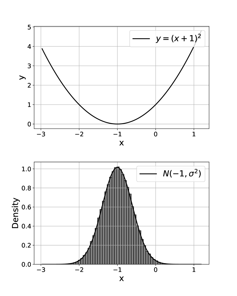
(a) Unconstrained Stochastic Gradient Descent

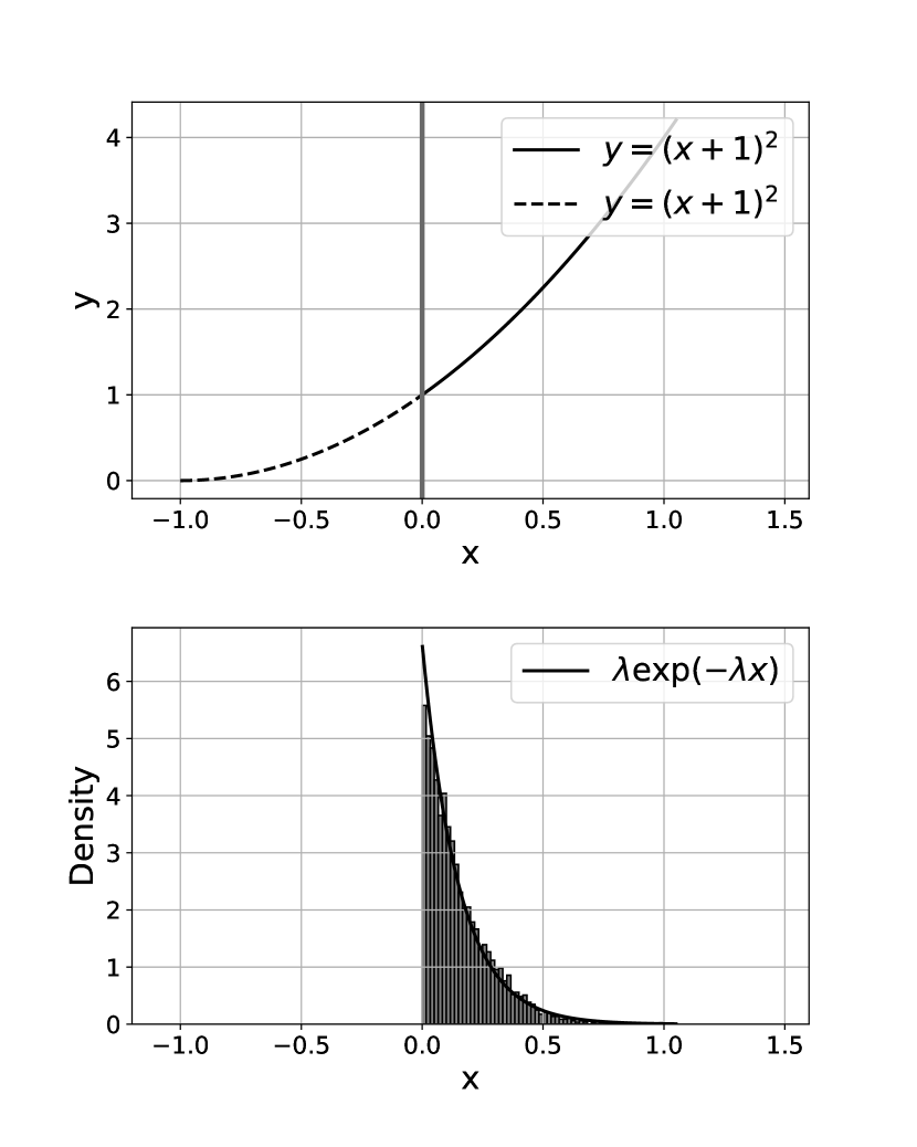
(b) Constrained Stochastic Gradient Descent

Figure 1: The above plots a simulation of a stochastic gradient descent algorithm with a constant step size on the function $f(x)=(x+1)^{2}$. Figure 2(a): When the objective is unconstrained the density of the location of iterates is well approximated by a normal distribution with variance $\sigma^{2}=O(\alpha)$, where $\alpha$ is the step size of the algorithm. The distance to the optimum is $O(\alpha^{1/2})$. Figure 2(b): When the value of $x$ is constrained to the positive orthant the gradient no longer vanishes. The distribution of iterates away from zero now has an exponential decay with rate $\lambda=O(\alpha^{-1})$. So for step size, $\alpha$, the distance to the optimum is $O(\alpha)$. This paper proves that exponential concentration holds more generally for stochastic approximation procedures with non-vanishing gradients.

With reference to Figure 1, the high-level intuition for this behavior in a stochastic gradient algorithm is as follows. Consider a projected stochastic gradient descent algorithm with a small but fixed learning rate. When the optimum is in the interior of the constraint set and the objective is smooth, the progress of the algorithm will slow as the iterates approach the minimizer in a manner that is roughly proportional to the distance to the optimum. In this regime, the process behaves is approximated by an Ornstein-Uhlenbeck (OU) process, for instance, see Chapter 10 of Kushner and Yin (2003). An OU process is known to have a normal distribution as its limiting stationary distribution. This stationary distribution determines the rate of convergence to the optimum, see Chen et al. (2022). If we consider the same iterates but instead these are now projected to belong to a constraint set (such as polytope) then, assuming that the optimum is on the boundary, the resulting process behaves in a manner that is approximated by a reflected Brownian motion. When the gradient is non-zero on the boundary, it is well known that a reflected Brownian motion with negative drift has an exponential distribution as its stationary distribution, see Harrison and Williams (1987). We seek to establish bounds that exhibit this exponential stationary behavior while allowing for time-dependent step sizes. This provides intuition for the exponential concentration results found in this paper.

3.2 An Exponential Lyapunov Bound

We state our first result below. When the slope of the objective function is bounded away from zero, a stochastic gradient descent algorithm will expect to always make progress towards minimizing its objective proportional to the learning rate $\alpha_{t}$. This leads to the following two conditions.

Drift Condition. The sequence $\{\bm{x}_{t}\}_{t=0}^{\infty}$ satisfies

$$\mathbb{E}[f(\bm{x}_{t+1})-f(\bm{x}_{t})|\mathcal{F}_{t}]\leq-2\alpha_{t}\kappa$$ (C1)

whenever $f(\bm{x}_{t})-f(\bm{x}^{\star})\geq\alpha_{t}B$ for some $\kappa>0$ and some $B>0$.

Moment Condition. There exists a constant $\eta>0$ and a random variable $Y$ such that

$$\big{[}|f(\bm{x}_{t+1})-f(\bm{x}_{t})|\big{|}\mathcal{F}_{t}\big{]}\leq\alpha_{t}Y\quad\text{and}\quad\mathbb{E}[e^{\alpha_{0}\eta Y}]<\infty\,.$$ (C2)

Condition (C1) states that the stochastic iterates will make progress against its objective when away from the optimum. The Condition (C2) is a mild noise condition. For example, if $f(X)$ is Lipschitz continuous then it is sufficient that $||\bm{c}_{t}||$ has a sub-exponential tail. (See Lemma 5 in Section A.1 for verification of this claim.) Shortly we will establish the Conditions (C1) and (C2) when applying projected stochastic gradient descent. However, for now, we leave (C1) and (C2) as general conditions that can be satisfied by a stochastic approximation algorithm.

The main result of this section is as follows.

Theorem 1.

For learning rates of the form $\alpha_{t}={a}/{(u+t)^{\gamma}}$ with $a,u>0$ and $\gamma\in[0,1]$, if Conditions (C1) and (C2) are satisfied by a stochastic approximation algorithm, then

$$\mathbb{P}(f(\bm{x}_{t+1})-f(\bm{x}^{\star})\geq z)\leq I{e^{-t^{\gamma}{J}z}}\,$$ (2)

and

$$\mathbb{E}[f(\bm{x}_{t+1})-f(\bm{x}^{\star})]\leq\frac{K}{t^{\gamma}}\,$$ (3)

for time independent constants $I$, $J$ and $K$.

What we see in these results is that once the dependence on the initial state of the system has been accounted for then the process $f(\bm{x}_{t})$ has an exponential concentration and will be within a factor of $\alpha_{t}$ of the optimum. This is proved in a more general form in Proposition 1 in Section 4.1.

It is worth remarking that Theorem 1 (and Proposition 1) hold for any algorithm for which the generic Conditions (C1) and (C2) hold. Thus the results are not intended to be applicable to any one particular stochastic gradient descent algorithm, nor do we place specific design restrictions on the algorithm. The result emphasizes that a convergence rate may differ depending on the geometry of the problem at hand, and this convergence may well be faster than that anticipated.

3.3 Projected Stochastic Gradient Descent

In the proof of Proposition 1 and Theorem 1, we did not specify the stochastic approximation procedure used nor did we explore settings where the key Conditions (C1) and (C2) hold. The purpose of this section is to provide a standard setting that allows for the application of our results. We consider projected stochastic gradient descent on the Lipschitz continuous function $l:\mathcal{\mathcal{missing}}X\rightarrow\mathbb{R}$. That is we wish to solve the optimization problem:

$$\text{minimize}\qquad l(\bm{x})\qquad\text{over}\quad x\in\mathcal{X}\,,$$ (4)

and we consider the Project Stochastic Gradient Descent (PSGD) algorithm:

$${\bm{y}}_{t+1} =\bm{x}_{t}-\alpha_{t}\bm{c}_{t}\,$$ (5a)

$$\bm{x}_{t+1} =\Pi_{\mathcal{X}}({\bm{y}}_{t+1})$$ (5b)

where $\mathbb{E}\big{[}\bm{c}_{t}\big{|}\mathcal{F}_{t}\big{]}=\nabla l(\bm{x}_{t})\,\text{and}\,\alpha_{t}=\frac{a}{(u+t)^{\gamma}}$ for $a>0$, $u\in\mathbb{R}_{+}$, $\gamma\in[0,1]$. Above $\nabla l(\bm{x})$ can be either the gradient or a sub-gradient of $l$. We let $\mathcal{X}^{\star}=\operatorname*{argmin}_{\bm{x}\in\mathcal{X}}l(\bm{x})$ be the set of optimizers.

Previously, we required Conditions (C1) and (C2) which place assumptions on the iterates and objective jointly. Now that we have specified the iterative procedure, we can decouple to give conditions that only depend on the properties of the objective function.
 Gradient Condition. There exists a positive constant $\kappa>0$ such that for all $\bm{x}\in\mathcal{X}$

$$\nabla l(\bm{x})^{\top}(\bm{x}-\bm{x}^{\star})\geq\kappa\|\bm{x}-\bm{x}^{\star}\|,\qquad$$ (D1)

where $\bm{x}^{\star}\in\Pi_{\mathcal{X}^{\star}}(\bm{x})$ and $\mathcal{X}^{\star}=\operatorname*{argmin}_{\bm{x}\in\mathcal{X}}l(\bm{x})$ .

Sub-Exponential Noise. There exists a $\lambda>0$ such that

$$\sup_{t\in\mathbb{N}}\mathbb{E}[e^{\lambda||\bm{c}_{t}||}|\mathcal{F}_{t}]<\infty\,.$$ (D2)

Conditions (D1) and (D2) replace Conditions (C1) and (C2). Let’s interpret these new conditions. Firstly, (D1) states that the (unit) directional derivative in the direction from $\bm{x}$ to $\bm{x}^{\star}$ is bounded above by $-\kappa$. (See Figure 2.) Condition (D2) assumes that the tail behavior of the gradient estimates is sub-exponential. (See Lemma 5.)

Remark 1.

(Convexity and Sharpness.) We don’t assume that $l(\bm{x})$ is convex but if it is then

$$\nabla l(\bm{x})^{\top}(\bm{x}-\bm{x}^{\star})= (\nabla l(\bm{x})-\nabla l(\bm{x}^{\star}))^{\top}(\bm{x}-\bm{x}^{\star})+\nabla l(\bm{x}^{\star})^{\top}(\bm{x}-\bm{x}^{\star})\,\geq\,\nabla l(\bm{x}^{\star})^{\top}(\bm{x}-\bm{x}^{\star})\,.$$

Thus assuming convexity a sufficient condition for (D1) to hold is that for all $\bm{x}\in\mathcal{X}$ there exists a sub-gradient $\nabla l(\bm{x}^{\star})$ at $\bm{x}^{\star}$ such that

$$\nabla l(\bm{x}^{\star})^{\top}(\bm{x}-\bm{x}^{\star})\geq\kappa||\bm{x}^{\star}-\bm{x}||\,.$$ (D1^′)

This implies that there is a non-vanishing slope away from the optimum. I.e. the function $l(\bm{x})$ belongs to a cone emanating from the set of optimal points. This condition is sometimes referred to as the sharp condition. So convexity and sharpness imply the gradient condition (D1).

Remark 2 (Projection).

PSGD requires a stochastic gradient descent step (5a) and a projection step (5b). We discuss the projection step. Projection is a common requirement in gradient descent algorithms, indeed almost all results on online convex optimization require some form of projection (see Hazan et al. (2016)). Nonetheless, it can present some computational overhead, so we discuss that here. First, results such as the Robbins-Sigmund Theorem ensure almost sure convergence of $\bm{x}_{t}$ to the set $\mathcal{X}^{*}$ (Robbins and Siegmund (1971)). Thus if $\mathcal{X}^{\star}$ belongs to the interior of $\mathcal{X}$ then eventually the algorithm does not require projection.

It is a common device that iterates are bounded to a set $\mathcal{X}$ that allows simple projection e.g. a box or circle containing $\mathcal{X}^{\star}$. In instances where the optimum belongs to the boundary of $\mathcal{X}$ projection cannot be avoided; however, we note that a number of common constraint sets have simple projections. For $\bm{g}:\mathbb{R}^{p}\rightarrow\mathbb{R}^{d}$, the dual of a constrain set $\{\bm{z}:\bm{g}(\bm{z})\leq 0\}$ is $\mathbb{R}^{d}_{+}=\{\bm{x}:\bm{x}\geq 0\}$ and thus allows for simple constraints that require projection and thus readily leads to the use of projected stochastic gradient descent on the dual. Thus for linear constraints $\{\bm{z}:A\bm{z}\leq\bm{b}\}$ linear programming (on the dual LP) is an important case for the application of our results. Low complexity projections exist of single constraint problems such as projection onto the probability simplex (Michelot (1986); Duchi et al. (2008)). Chapter 7 gives a number of examples of fast projection available with conditional gradient algorithms Hazan et al. (2016). See also Bertsekas (2015) for further examples of low complexity projection.

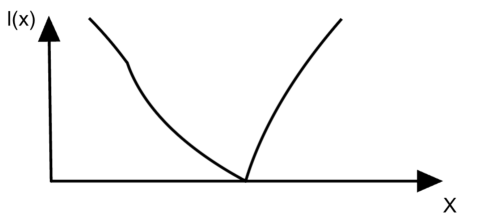
(a) Gradient Condition (D1).

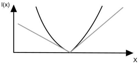
(b) Convexity and Sharpness (D1^′)

Figure 2: Under the gradient condition (D1), the objective need not be convex nor continuously differentiable. We require the derivative in the direction of the optimum to be non-zero. Under convexity and sharpness (D1^′), there is a cone around the optimum, and condition (D1) is satisfied.

We can prove the following result that holds as a consequence of Theorem 1.

Theorem 2.

If condition (D1) and (D2) hold then projected stochastic gradient descent satisfies

$$\mathbb{P}\left(\min_{\bm{x}\in\mathcal{X}}\left\|\bm{x}_{t+1}-\bm{x}\right\|\geq z\right)\leq Je^{-It^{\gamma}z},\quad\mathbb{E}\left[\min_{\bm{x}\in\mathcal{X}}\left\|\bm{x}_{t+1}-\bm{x}\right\|\right]\leq\frac{K}{t^{\gamma}},\quad and\quad\mathbb{E}\left[l(\bm{x}_{t+1})-\min_{\bm{x}\in\mathcal{X}}l(\bm{x})\right]\leq\frac{L}{t^{\gamma}}\,$$

where above $J,I,K,L$ are positive constants.

For Stochastic Gradient Descent (SGD), the expected distance from $\bm{x}_{t}$ to the set of optima $\mathcal{X}^{\star}$ is known to converge at rate $\Omega(1/\sqrt{t})$ (both with and without strong convexity and with and without Polyak-Ruppert averaging). Thus the rate of convergence found in Theorem 2 is faster than that typically assumed for SGD. Thus we see that a tight concentration occurs around the optimum in such cases. Although the Gaussian concentration around the optimum for strongly convex objectives is well understood, to the best of our knowledge the exponential concentration found here does not appear in prior work on PSGD.

3.4 Linear Convergence of PSGD with Non-vanishing Gradient.

The linear convergence of Projected Stochastic Gradient Descent (PSGD) on convex objectives is established in Theorem 3.2 of Davis et al. (2019). This result relies on a general concentration result (Davis and Drusvyatskiy, 2019, Theorem 4.1) which is not as tight as Theorem 2 above. Thus below in Theorem 3, we provide improvements to some results in Davis et al. (2019).

We wish to solve the optimization problem (4). We consider the PSGD algorithm (5) implemented over a number of stages, $s=1,...,S$. We let $t_{s}$ be the number of iterations in the $s$th stage. The idea is that within each stage $s$ the learning rate $\hat{\alpha}_{s}$ is fixed, and is chosen so that the error of the stochastic approximation algorithm should be halved by the end of each stage. Specifically, we let $\hat{\bm{x}}_{s}$ be the state at the end of stage $s$. For $s=1,...,S$ , we take $\alpha_{s}>0$ and $t_{s}\in\mathbb{N}$ and we define $T_{s}=\sum_{s^{\prime}=1}^{s}t_{s^{\prime}}$. For $t$ and $s$, we define

$$\hat{\bm{x}}_{s} =\bm{x}_{T_{s}},\qquad\text{and}\qquad\alpha_{t}=\hat{\alpha}_{s},\qquad T_{s-1}\leq t<T_{s}\,.$$ (6a)

The following theorem gives choices for $\hat{\alpha}_{s}$ and $t_{s}$ to ensure a linear rate of convergence.

Theorem 3.

Assume Conditions (D1) and (D2) hold. For PSGD, (5), with rates given in (6):

a) If, for $\hat{\epsilon}>0$ and $\hat{\delta}\in(0,1)$, we set

$$S=\log\left(\frac{F}{\hat{\epsilon}}\right),\quad\hat{\alpha}_{s}=\frac{2^{-s}F\kappa}{E\log\Big{(}\frac{GS}{\hat{\delta}}\Big{)}},\quad\text{and}\quad t_{s}=\left\lceil\frac{2}{\kappa^{2}}\log\left(\frac{GS}{\hat{\delta}}\right)\right\rceil$$

then with probability greater than $1-\hat{\delta}$ it holds that $\min_{\bm{x}\in\mathcal{X}^{\star}}\left\|\hat{\bm{x}}_{S}-\bm{x}\right\|\leq\hat{\epsilon}\,.$ Moreover the number of iterations (6) required to achieve this bound is

$$\Big{\lceil}\log_{2}\Big{(}\frac{F}{\hat{\epsilon}}\Big{)}\Big{\rceil}\left\lceil\frac{2}{\kappa^{2}}\log\left(\frac{G}{\hat{\delta}}\right)+\log\Big{(}\Big{\lceil}\log_{2}\Big{(}\frac{F}{\hat{\epsilon}}\Big{)}\Big{\rceil}\Big{)}\right\rceil\,.$$

b) For $\hat{\alpha}_{s}=\frac{a}{2^{s}\log(s+1)}$ and $t_{s}=\log^{2}(s+1)$, there exists positive constants $A$ and $M$ such that $\forall\hat{\delta}\in(0,1)$ if $a\geq A/\hat{\delta}$ then

$$\mathbb{P}\left(\min_{\bm{x}\in\mathcal{X}^{\star}}\|\hat{\bm{x}}_{s}-\bm{x}\|\leq 2^{-s}M,\quad\forall s\in\mathbb{N}\right)\geq 1-\hat{\delta}\,.$$

The bound in Theorem 3a) above has an order $O(\log\hat{\epsilon}^{-1}\big{[}\log\log\hat{\epsilon}^{-1}+\log\hat{\delta}^{-1}\big{]})$. The above bound is the same order as the best bound found in Davis et al. (2019), namely Theorem 3.8, which holds for an ensemble method consisting of three adaptively regularized gradient descent algorithms.

Unlike Theorem 2, Theorem 3a) suggests that we require a refined understanding to calibrate parameters to improve convergence. The implementation of Theorem 3b) only requires one parameter, $a$, which needs to chosen sufficiently large. (For instance, experiments could increase the parameter $a$ until convergence is observed.) Thus, although the complexity of part b) is worse than a), we do not require detailed knowledge of the problem at hand to implement a geometrically convergent algorithm. Further, Theorem 3b) holds for a stronger mode of convergence, in that the geometric convergence holds for all time with arbitrarily high probability.

3.5 The Exponential Approximation

The limit distribution of stochastic approximation is normal when the shape of the objective around the optimum is approximately quadratic. In our case, the curvature is linear, and our analysis proves exponential tail behavior. A natural question is if the limiting distribution of iterates away from the optimum are exponentially distributed under the constant drift condition? That is do we have convergence in distribution ${x_{t}}/{\alpha_{t}}\xrightarrow[]{\mathcal{D}}X,$ as $t\rightarrow\infty$ where $X$ is exponentially distributed? The short answer is no. In general, the limit distribution is not exponential.

For a simple counter-example, consider projected stochastic gradient descent where $\mathcal{X}=\mathbb{R}_{+}$ and $c_{t}$ are i.i.d. random variables with $c_{t}=-1$ with probability $p$ and $c_{t}=1$ with probability $1-p$. If we fix $\alpha$, we can already see that an exponential distribution limit is not possible, since the process $x_{t}/\alpha$ belongs to the set $\mathbb{Z}_{+}$. If $p>1/2$, then the limit distribution is geometrically distributed, not exponential. For general distributions of $c_{t}$, the limit distribution is given by an integral equation. (See Lindley’s Integral Equation (Asmussen, 2003, Corollary 6.6).) However, the resulting distributions all exhibit exponential tail bounds. (See Kingman’s Bound c.f. Kingman (1964))

Convergence in distribution likely holds. However, the limit $X$ is unlikely to be exponential, and it is unlikely to have a simple form. We cannot expect a simple statistic like the Fisher Information to determine the directions of statistical error because the stochastic approximation process is much more concentrated. Thus we can not aggregate fluctuations in the same manner as found in the normal approximation. Errors and stepsizes are of the same order of magnitude, which is one reason why exponential tail bounds are not commonplace in prior literature on stochastic approximation. However, as we see in this article, we can understand convergence behavior by constructing these exponential concentration bounds.

4 Proofs

4.1 Proof of Theorem 1

The proof of Theorem 1 relies on the following proposition. This result establishes that once the sum $\sum_{s=1}^{t}\alpha_{s}$ is sufficiently large, the error of stochastic iterations is of the order of $\alpha_{t}$. For the stochastic iterates described in Section 2, we will assume that $\{\alpha_{t}\}_{t\geq 0}$ is a deterministic non-increasing sequence such that

$$\sum_{t=0}^{\infty}\alpha_{t}=\infty,\qquad\liminf_{t\rightarrow\infty}\,\frac{\alpha_{2t}}{\alpha_{t}}>0\qquad\text{and }\qquad\lim_{t\rightarrow\infty}\frac{\alpha_{t}-\alpha_{t+1}}{\alpha_{t}}=0\,.$$ (7)

We do not need to assume that $\alpha_{t}\rightarrow 0$. Later we consider small but constant step sizes. This condition is satisfied by any sequence of the form $\alpha_{t}=a/(b+t)^{\gamma}$ for $a,b>0$ and $\gamma\in[0,1]$.

Proposition 1.

When Conditions (C1) and (C2) are satisfied, there exist positive constants $E,G,H$ such that

$$\mathbb{P}(f(\bm{x}_{t+1})-f(\bm{x}^{\star})\geq z)\leq e^{-\frac{\kappa G^{n}}{2E\alpha_{t}}(z-\alpha_{t}B-F-\alpha_{0}B+\sum_{s=\lfloor t/2^{n}\rfloor}^{t}\alpha_{s}\frac{\kappa}{2})}+H{e^{-\frac{\kappa G^{n}}{2E\alpha_{t}}(z-\alpha_{t}B)}}\,.$$ (8)

for any $n$ with $t/2^{n}>1$. Further, for any $t$ such that $\sum_{s=\lfloor t/2^{n}\rfloor}^{t}\alpha_{s}\kappa\geq 2(F+\alpha_{0}B)$ there exists a constant $C$ such that

$$\mathbb{E}[f(\bm{x}_{t+1})-f(\bm{x}^{\star})]\leq C\alpha_{t}\,.$$ (9)

4.1.1 Proof of Proposition 1

Let’s briefly outline the proof of Proposition 1. The proof uses Lemma 1, Lemma 2, Lemma 3, and Proposition 2, which are stated below. Lemma 1, although not critical to our analysis, simplifies the drift Condition (C1) by eliminating some terms and boundary effects. Lemma 2, on the other hand, is a critical component of our proof. It converts the linear drift Condition (C1) into an exponential bound which we then iteratively expand. The lemma extends Theorem 2.3 from Hajek (1982) by allowing for adaptive time-dependent step sizes. Proposition 2 applies standard moment generating function inequalities to the results found in Lemma 2. Lemma 3 is a technical lemma used in the proof of Proposition 2. After Proposition 2 is proven, the proof of Proposition 1 follows.

We now proceed with the steps outlined above. We let

$$L_{t}:=f(\bm{x}_{t})-f(\bm{x}^{\star})-\alpha_{t}B$$ (10)

where $\alpha_{t}$ satisfies (7). First, we simplify the above Conditions (C1) and (C2) to give the Lyapunov conditions (11) and (12) stated below. The following is a technical lemma.

Lemma 1.

Given Conditions (C1) and (C2) hold, there exists a constant deterministic constant $t_{0}$ such that the sequence of random variables $(L_{t}:t\geq t_{0})$ satisfies

$$\mathbb{E}\big{[}L_{t+1}-L_{t}\big{|}\mathcal{F}_{t}\big{]}\mathbb{I}[L_{t}\geq 0]<-\alpha_{t}\kappa,$$ (11)

and

$$[|L_{t+1}-L_{t}||\mathcal{F}_{t}]\leq\alpha_{t}Z\quad\text{where}\quad D:=\mathbb{E}[e^{\alpha_{0}\eta Z}]<\infty\,.$$ (12)

The proof is in Section A.2.

Now given (12) holds, we will convert the drift condition (11) into an exponential bound and then iterate to give the bound below.

Lemma 2.

$$\mathbb{E}[e^{\eta L_{t+1}}]\leq\mathbb{E}[e^{\eta L_{t_{1}}}]\prod_{k=t_{1}}^{t}\rho_{t}+D\sum_{\tau=t_{1}+1}^{t+1}\prod_{k=\tau}^{t}\rho_{k}\,,$$

for $t\geq t_{1}\geq t_{0}$ where $\rho_{t}=e^{-\alpha_{t}\eta\kappa+\alpha_{t}^{2}\eta^{2}E}$, and $E=\mathbb{E}\left[({e^{\eta\alpha_{0}Z}-1-\alpha_{0}\eta Z})/{\eta^{2}}\right]<\infty$.

Proof.

(Proof of Lemma 2). Let $Z_{t}=(L_{t+1}-L_{t})/\alpha_{t}$. From (12), we have $[|Z_{t}||\mathcal{F}_{t}]\leq Z$ where $\mathbb{E}[e^{\eta\alpha_{0}Z}]<\infty$. From (11), we have $\mathbb{E}[Z_{t}|\mathcal{F}_{t}]\leq-\kappa$ on the event $\{L_{t}\geq 0\}$. Thus, on the event $\{L_{t}\geq 0\}$ the following holds:

$$\mathbb{E}[e^{\eta(L_{t+1}-L_{t})}|\mathcal{F}_{t}]=\mathbb{E}[e^{\alpha_{t}\eta Z_{t}}|\mathcal{F}_{t}] =1+\alpha_{t}\eta\mathbb{E}[Z_{t}|\mathcal{F}_{t}]+\alpha_{t}^{2}\eta^{2}\mathbb{E}\left[\frac{e^{\alpha_{t}\eta Z_{t}}-1-\alpha_{t}\eta Z_{t}}{\alpha_{t}^{2}\eta^{2}}\Big{|}\mathcal{F}_{t}\right]$$

$$=1+\alpha_{t}\eta\mathbb{E}[Z_{t}|\mathcal{F}_{t}]+\alpha_{t}^{2}\eta^{2}\sum_{k=2}^{\infty}\frac{1}{k!}\mathbb{E}[Z_{t}^{k}|\mathcal{F}_{t}]\eta^{k-2}\alpha_{t}^{k-2}$$

$$\leq 1-\alpha_{t}\eta\kappa+\alpha_{t}^{2}\eta^{2}\sum_{k=2}^{\infty}\frac{1}{k!}\mathbb{E}[Z^{k}]\eta^{k-2}\alpha_{0}^{k-2}$$

$$=1-\alpha_{t}\eta\kappa+\alpha_{t}^{2}\eta^{2}\mathbb{E}\left[\frac{e^{\eta\alpha_{0}Z}-1-\alpha_{0}\eta Z}{\eta^{2}}\right]$$ (13)

$$=1-\alpha_{t}\eta\kappa+\alpha_{t}^{2}\eta^{2}E$$

$$\leq e^{-\alpha_{t}\eta\kappa+\alpha_{t}^{2}\eta^{2}E}=:\rho_{t}\,.$$ (14)

In the first equality above, we apply a Taylor expansion. In the first inequality, we apply (11) and (12) above, and also recall that $\alpha_{t}$ is decreasing. In the final inequality, we applied the standard bound $1+x\leq e^{x}$. We note that $\rho_{t}$ as define above satisfies $\rho_{t}<1$ whenever $\alpha_{t}<{\kappa}/{\eta E}$. We note that $E$ is finite since by assumption $\mathbb{E}[e^{\eta\alpha_{0}Z}]<\infty$. Also from the expansion given in (13), it is clear that $E$ is positive.

The bound (14) holds on the event $\{L_{t}\geq 0\}$. Now notice

$$\mathbb{E}[e^{\eta L_{t+1}}|\mathcal{F}_{t}] =\mathbb{E}[e^{\eta(L_{t+1}-L_{t})}|\mathcal{F}_{t}]e^{\eta L_{t}}\mathbb{I}[L_{t}\geq 0]+\mathbb{E}[e^{\eta(L_{t+1}-L_{t})}|\mathcal{F}_{t}]e^{\eta L_{t}}\mathbb{I}[L_{t}<0]$$

$$\leq\rho_{t}e^{\eta L_{t}}\mathbb{I}[L_{t}\geq 0]+\mathbb{E}[e^{\alpha_{0}Z}]e^{\eta L_{t}}\mathbb{I}[L_{t}<0]$$

$$\leq\rho_{t}e^{\eta L_{t}}\mathbb{I}[L_{t}\geq 0]+D\mathbb{I}[L_{t}<0]$$

$$\leq\,\rho_{t}e^{\eta L_{t}}+D\,.$$

The first inequality applies the above bound (14) and the second inequality applies the boundedness condition (12). Taking expectations above gives

$$\mathbb{E}[e^{\eta L_{t+1}}]\leq\rho_{t}\mathbb{E}[e^{\eta L_{t}}]+D.$$

By induction, we have

$$\mathbb{E}[e^{\eta L_{t+1}}]\leq\mathbb{E}[e^{\eta L_{t_{1}}}]\prod_{k=t_{1}}^{t}\rho_{t}+D\sum_{\tau=t_{1}+1}^{t+1}\prod_{k=\tau}^{t}\rho_{k}\,,$$

as required. ∎

The following is a technical lemma.

Lemma 3.

If $\alpha_{t}$, $t\in\mathbb{Z}_{+}$, is a decreasing positive sequence, then

$$\min_{s=t_{1},...,t}\left\{\frac{\sum_{k=s}^{t}\alpha_{k}}{\sum_{k=s}^{t}\alpha_{k}^{2}}\right\}=\frac{\sum_{k=t_{1}}^{t}\alpha_{k}}{\sum_{k=t_{1}}^{t}\alpha_{k}^{2}}\,.$$ (15)

Moreover, if $\alpha_{t}$, $t\in\mathbb{Z}_{+}$ satisfies the learning rate condition (7) then

$$\min_{s=\lfloor t/2^{n}\rfloor,...,t}\left\{\frac{\sum_{k=s}^{t}\alpha_{k}}{\sum_{k=s}^{t}\alpha_{k}^{2}}\right\}\geq\frac{G^{n}}{\alpha_{t}}$$ (16)

for some positive constant $G$ and for $n\in\mathbb{N}$ such that $t/2^{n}>1$.

The proof is in Section A.2.

With the moment generating function bound in Lemma 2 and the bound in Lemma 3, we can bound the tail probabilities and expectation of $L_{t}$.

Proposition 2.

For any sequence satisfying (7), there exists a constant $H$ such that

$$\mathbb{P}(L_{t+1}\geq z)\leq \ e^{-\frac{\kappa G^{n}}{2E\alpha_{t}}(z-F-\alpha_{0}B+\sum_{s=\lfloor t/2^{n}\rfloor}^{t}{\alpha}_{s}\frac{\kappa}{2})}+H{e^{-\frac{\kappa G^{n}}{2E\alpha_{t}}z}}\$$ (17)

for $z\geq 0$. Further, for $t$ is such that $\sum_{s=1}^{t}{\alpha}_{s}\frac{\kappa}{2}\geq F+\alpha_{0}B$, then

$$\mathbb{E}[L_{t+1}]\leq\frac{2\left(1+H\right)E}{G^{n}\kappa}\alpha_{t}\,.$$

Proof.

(Proof of Proposition 2). We apply Lemma 2 with $t_{1}=\lfloor t/2^{n}\rfloor$ which gives

$$\mathbb{P}(L_{t+1}\geq z) \leq e^{-\eta z}\mathbb{E}[e^{\eta L_{t+1}}]$$

$$\leq e^{-\eta z}\mathbb{E}[e^{\eta L_{t_{1}}}]\prod_{k=t_{1}}^{t}\rho_{t}+e^{-\eta z}D\sum_{\tau=t_{1}+1}^{t+1}\prod_{k=\tau}^{t}\rho_{k}$$

$$=e^{-\eta z}\mathbb{E}[e^{\eta L_{t_{1}}}]e^{\sum_{k=t_{1}}^{t}-\alpha_{k}\eta\kappa+\alpha_{k}^{2}\eta^{2}E}+e^{-\eta z}D\sum_{\tau=t_{1}+1}^{t+1}e^{\sum_{k=\tau}^{t}-\alpha_{t}\eta\kappa+\alpha_{t}^{2}\eta^{2}E}\ .$$ (18)

We let $\eta$ be such that $0\leq\eta\leq\min_{t_{1}\leq s\leq t}\left\{\frac{\sum_{k=s}^{t}\alpha_{k}\kappa}{2\sum_{k=s}^{t}\alpha_{k}^{2}E}\right\}$. Notice, for such $\eta$, it holds that

$$\sum_{k=\tau}^{t}-\alpha_{k}\eta\kappa+\alpha_{k}^{2}\eta^{2}E\leq-\frac{1}{2}\sum_{k=\tau}^{t}\alpha_{k}\eta\kappa\leq-\frac{1}{2}(t-\tau)\alpha_{\tau},\qquad\forall\tau=t_{1},...,t\ .$$

Applying this to (18) gives

$$\mathbb{P}(L_{t+1}\geq z) \leq e^{-\eta z}\mathbb{E}[e^{\eta L_{t_{1}}}]e^{\sum_{k=t_{1}}^{t}-\alpha_{k}\eta\frac{\kappa}{2}}+e^{-\eta z}D\sum_{\tau=t_{1}+1}^{t+1}e^{-(t-\tau)\alpha_{k}\eta\frac{\kappa}{2}}$$

$$\leq e^{-\eta z}\mathbb{E}[e^{\eta L_{t_{1}}}]e^{\sum_{k=t_{1}}^{t}-\alpha_{k}\eta\frac{\kappa}{2}}+e^{-\eta z}D\frac{e^{\alpha_{t}\eta\frac{\kappa}{2}}}{1-e^{-\alpha_{t}\eta\frac{\kappa}{2}}}$$ (19)

In the 2nd inequality above we note that $\alpha_{k}\geq\alpha_{t}$ for all $k\leq t$. In the 3rd inequality, we note that the summation over $\tau$ are terms from a geometric series, so we upper bound this by the appropriate infinite sum.

By Lemma 3, we see that

$$\min_{t_{1}\leq s\leq t}\left\{\frac{\sum_{k=s}^{t}\alpha_{k}\kappa}{2\sum_{k=s}^{t}\alpha_{k}^{2}E}\right\}=\frac{\kappa}{2E}\frac{\sum_{k=t_{1}}^{t}\alpha_{k}}{\sum_{k=t_{1}}^{t}\alpha_{k}^{2}}\geq\frac{\kappa G^{n}}{2\alpha_{t}E}$$

for a constant $G>0$. In particular, we take $\eta=\kappa G^{n}/2E\alpha_{t}$. Thus, the bound (19) becomes

$$\mathbb{P}(L_{t+1}\geq z)\leq\mathbb{E}\Big{[}e^{\frac{\kappa G^{n}L_{t_{1}}}{2E\alpha_{t}}}\Big{]}e^{-\frac{\kappa G^{n}}{2E\alpha_{t}}(z+\sum_{s=t_{1}}^{t}{\alpha}_{s}\frac{\kappa}{2})}+e^{-\frac{\kappa G^{n}}{2E\alpha_{t}}z}D\frac{e^{\frac{\kappa^{2}G^{n}}{4E}}}{1-e^{-\frac{\kappa^{2}G^{n}}{4E}}}\ .$$

Noting that $L_{t_{1}}\leq\max_{x\in\mathcal{X}}f(x)-\min_{x\in\mathcal{X}}f(x)+\alpha_{0}B=F+\alpha_{0}B$, by the definition of $F$. We simplify the above expression as follows

$$\mathbb{P}(L_{t+1}\geq z)\leq \,e^{\frac{\kappa G^{n}}{2E\alpha_{t}}[F+\alpha_{0}B-z-\sum_{s=\lfloor t/2^{n}\rfloor}^{t}{\alpha}_{s}\frac{\kappa}{2}]}+e^{-\frac{\kappa G^{n}}{2E\alpha_{t}}z}D\frac{e^{\frac{\kappa^{2}G^{n}}{4E}}}{1-e^{-\frac{\kappa^{2}G^{n}}{4E}}}$$

$$\leq \ e^{-\frac{\kappa G^{n}}{2E\alpha_{t}}(z+\sum_{s=\lfloor t/2^{n}\rfloor}^{t}{\alpha}_{s}\frac{\kappa}{2}-F-\alpha_{0}B)}+H{e^{-\frac{\kappa G^{n}}{2E\alpha_{t}}z}}\ .$$ (20)

Above we define $H:=D{e^{\frac{\kappa^{2}G^{n}}{4E}}}/{(1-e^{-\frac{\kappa^{2}G^{n}}{4E}})}$. This gives (17).

Notice if $t$ is such that $F+\alpha_{0}B-\sum_{s=\lfloor t/2^{n}\rfloor}^{t}\hat{\alpha}_{s}\frac{\kappa}{2}\leq 0$, then the above inequality (20) can be bounded by

$$\mathbb{P}(L_{t+1}\geq z)\leq\left(1+H\right)e^{-\frac{\kappa G^{n}}{2E\alpha_{t}}z}.$$

Thus

$$\mathbb{E}[L_{t+1}] \leq\mathbb{E}[L_{t+1}\vee 0]=\int_{0}^{\infty}\mathbb{P}(L_{t+1}\geq z)dz\leq(1+H)\int_{0}^{\infty}e^{-\frac{\kappa G^{n}}{2E\alpha_{t}}z}\,dz=2\left(1+H\right)\frac{\alpha_{t}E}{\kappa G^{n}}\ ,$$

as required. ∎

With Proposition 2 in place we can prove Proposition 1.

Proof.

(Proof of Proposition 1). From Proposition 2

$$\mathbb{P}(L_{t+1}\geq z^{\prime})\leq \ e^{-\frac{\kappa G^{n}}{2E\alpha_{t}}(z^{\prime}-F-\alpha_{0}B+\sum_{s=\lfloor t/2^{n}\rfloor}^{t}\alpha_{s}\frac{\kappa}{2})}+H{e^{-\frac{\kappa G^{n}}{2E\alpha_{t}}z^{\prime}}}\$$

for $z^{\prime}\geq 0$ where $f(\bm{x}_{t+1})=L_{t+1}+\alpha_{t+1}B+f(\bm{x}^{\star})$. Taking $z^{\prime}=z-\alpha_{t+1}B$, gives

$$\mathbb{P}(f(\bm{x}_{t+1})-f(\bm{x}^{\star})\geq z) =\mathbb{P}(L_{t+1}\geq z-\alpha_{t+1}B)$$

$$\leq e^{-\frac{\kappa G^{n}}{2E\alpha_{t}}(z-\alpha_{t}B-F-\alpha_{0}B+\sum_{s=\lfloor t/2^{n}\rfloor}^{t}\alpha_{s}\frac{\kappa}{2})}+H{e^{-\frac{\kappa G^{n}}{2E\alpha_{t}}(z-\alpha_{t}B)}}\,,$$

which gives (8) as required. Also by Proposition 2, we have

$$\mathbb{E}[f(\bm{x}_{t+1})-f(\bm{x}^{\star})]=\mathbb{E}[L_{t+1}]+\alpha_{t+1}B\; \leq\;2\left(1+H\right)\frac{\alpha_{t}E}{\kappa G^{n}}+\alpha_{t+1}B\leq\left[2\left(1+H\right)\frac{E}{\kappa G^{n}}+B\right]\alpha_{t}.$$

Thus taking $C=\left[2\left(1+H\right){E}/{2\kappa G^{n}}+B\right]$, the required bound (9) holds. ∎

4.1.2 Proof of Theorem 1

We consider the case $\gamma\in[0,1)$. The proof for $\gamma=1$ is very similar to avoid repetition we present its proof in the Section A.3.

Proof.

(Proof of Theorem 1 for $\gamma\in[0,1)$). When $\gamma\in[0,1)$ we take $n=1$ in Proposition 1. We first focus on achieving the bound $\sum^{t}_{s=\lfloor t/2^{n}\rfloor}\alpha_{s}\frac{\kappa}{2}\geq\alpha_{0}B+F\,.$. As this corresponds to the time period for the process to reach equilibrium behavior. Notice that

$$\sum_{s=\lfloor(v-u)/2^{n}\rfloor}^{v-u}\alpha_{s}= \sum_{s=\lfloor(v-u)/2^{n}\rfloor}^{v-u}\frac{a}{(u+s)^{\gamma}}\geq\,\int_{v/2-u}^{v-u}\frac{a}{(u+s)^{\gamma}}ds=\frac{a}{1-\gamma}\left[1-\frac{1}{2^{1-\gamma}}\right]v^{1-\gamma}\,.$$ (21)

When $t=v-u$ is such that

$$t\geq b+\frac{\alpha_{0}B+F}{\frac{a}{1-\gamma}\left[1-\frac{1}{2^{1-\gamma}}\right]}=:t_{1}\,,$$

then applied to the above bound, we have that $\sum^{t}_{s=\lfloor t/2^{n}\rfloor}\alpha_{s}\frac{\kappa}{2}\geq\alpha_{0}B+F\,.$ Thus applying bound (8) from Proposition 1 with $t_{2}=\max\{t_{0},t_{1}\}$, we see that

$$\mathbb{P}(f(\bm{x}_{t+1})-f(\bm{x}^{\star})\geq z)\leq(1+H){e^{-\frac{\kappa G}{2E\alpha_{t}}(z-\alpha_{t}B)}}\,\qquad\text{ for }t\geq t_{2}\,.$$

Thus we see that (2) holds for $t\geq 0$ with suitable choice of $I$ (e.g. $I=(1+H)e^{KG/2E(F/\alpha_{t_{2}}-B)}$). Integrating the bound (2) then gives

$$\mathbb{E}[f(\bm{x}_{t+1})-f(\bm{x}^{\star})]\leq\left[\frac{2EI}{\kappa G}+B\right]\alpha_{t}\,.$$

∎

4.2 Proof of Theorem 2

Proof.

(Proof of Theorem 2). In this proof, we will apply Proposition 1 with the choice $f(\bm{x}):=\min_{\bm{x}^{\star}\in\mathcal{X}^{\star}}\|\bm{x}-\bm{x}^{\star}\|\,.$ We also define $\bm{x}_{t}^{\star}:=\operatorname*{argmin}_{\bm{x}\in\mathcal{X}^{\star}}\|\bm{x}_{t}-\bm{x}\|$. Now observe that

$$f(\bm{x}_{t+1})^{2}=\left\|\bm{x}_{t+1}-\bm{x}_{t+1}^{\star}\right\|^{2}\leq\, \left\|\bm{x}_{t+1}-\bm{x}_{t}^{\star}\right\|^{2}=\,\left\|\Pi_{\mathcal{X}}(\bm{x}_{t}-\alpha_{t}\bm{c}_{t})-\Pi_{\mathcal{X}}(\bm{x}^{\star}_{t})\right\|^{2}$$

$$\leq\, \left\|\bm{x}_{t}-\alpha_{t}\bm{c}_{t}-\bm{x}^{\star}_{t}\right\|^{2}=\,\left\|\bm{x}_{t}-\bm{x}_{t}^{\star}\right\|^{2}-2\alpha_{t}\bm{c}_{t}^{\top}\left(\bm{x}_{t}-\bm{x}_{t}^{\star}\right)+\alpha_{t}^{2}\left\|\bm{c}_{t}\right\|^{2}\,.$$ (22)

The bound (D2) implies all moments of $\|\bm{c}_{t}\|$ are uniformly bounded. In particular, suppose $\sigma$ is such that $\mathbb{E}[\|\bm{c}_{t}\|^{2}|\mathcal{F}_{t}]<\sigma^{2}$. If $\bm{x}_{t}$ is such that $\|\bm{x}_{t}-\bm{x}^{\star}\|\geq\alpha_{t}\frac{\sigma^{2}}{\kappa}>0$ then

$$f(\bm{x}_{t+1})\leq\, \left\|\bm{x}_{t}-\bm{x}_{t}^{\star}\right\|\sqrt{1-2\alpha_{t}\bm{c}_{t}^{\top}\frac{\left(\bm{x}_{t}-\bm{x}_{t}^{\star}\right)}{\left\|\bm{x}_{t}-\bm{x}_{t}^{\star}\right\|^{2}}+\alpha_{t}^{2}\frac{\left\|\bm{c}_{t}\right\|^{2}}{\left\|\bm{x}_{t}-\bm{x}_{t}^{\star}\right\|^{2}}}$$

$$\leq\, \left\|\bm{x}_{t}-\bm{x}_{t}^{\star}\right\|\left(1-\alpha_{t}\bm{c}_{t}^{\top}\frac{\left(\bm{x}_{t}-\bm{x}_{t}^{\star}\right)}{\left\|\bm{x}_{t}-\bm{x}_{t}^{\star}\right\|^{2}}+\frac{\alpha_{t}^{2}}{2}\frac{\left\|\bm{c}_{t}\right\|^{2}}{\left\|\bm{x}_{t}-\bm{x}_{t}^{\star}\right\|^{2}}\right)\,.$$

Above the first inequality follows from (22) and in the second inequality we note that $\sqrt{1+x}\leq 1+\frac{x}{2}$. Taking expectations on both sides shows that, on the event $\{\|\bm{x}_{t}-\bm{x}^{\star}\|\geq\alpha_{t}\frac{\sigma^{2}}{\kappa}\}$, it holds that

$$\mathbb{E}\left[\left\|\bm{x}_{t+1}-\bm{x}_{t+1}^{\star}\right\||\mathcal{F}_{t}\right]\leq\, \left\|\bm{x}_{t}-\bm{x}_{t}^{\star}\right\|-\alpha_{t}\frac{\nabla l(\bm{x}_{t})^{\top}\left(\bm{x}_{t}-\bm{x}_{t}^{\star}\right)}{\left\|\bm{x}_{t}-\bm{x}_{t}^{\star}\right\|}+\frac{\alpha_{t}^{2}}{2}\frac{\mathbb{E}[\left\|\bm{c}_{t}\right\|^{2}|\mathcal{F}_{t}]}{\left\|\bm{x}_{t}-\bm{x}_{t}^{\star}\right\|}\leq\,\left\|\bm{x}_{t}-\bm{x}_{t}^{\star}\right\|-\alpha_{t}\kappa+\alpha_{t}\frac{\kappa}{2}$$

Or in other words $\mathbb{E}[f(\bm{x}_{t+1})-f(\bm{x}_{t})|\mathcal{F}_{t}]\leq-\alpha_{t}\frac{\kappa}{2}$ whenever $f(\bm{x}_{t})-f(\bm{x}^{\star})\geq\alpha_{t}\frac{\sigma^{2}}{\kappa}$. Thus we see that Condition (C1) holds.

We now verify Condition (C2). Since $\alpha_{t}$ is non-increasing and since projections reduce distances:

$$\mathbb{E}\left[\exp\left\{\frac{\eta}{\alpha_{1}}\left|f(\bm{x}_{t+1})-f(\bm{x}_{t})\right|\right\}\Big{|}\mathcal{F}_{t}\right]\leq\,\mathbb{E}\left[e^{\frac{\eta}{\alpha_{1}}\left\|\bm{x}_{t+1}-\bm{x}_{t}\right\|}\Big{|}\mathcal{F}_{t}\right]\leq\,\mathbb{E}\left[e^{\frac{\eta\alpha_{t}}{\alpha_{1}}\left\|\bm{c}_{t}\right\|}\Big{|}\mathcal{F}_{t}\right]\leq\mathbb{E}\left[e^{\eta\left\|\bm{c}_{t}\right\|}\big{|}\mathcal{F}_{t}\right]\,.$$

From the inequality above we see that Condition (C2) follows from Condition (D2).

We can now apply Theorem 1 which gives:

$$\mathbb{P}\Big{(}\min_{\bm{x}\in\mathcal{X}^{\star}}\left\|\bm{x}_{t+1}-\bm{x}\right\|\geq z\Big{)}\leq Ie^{-Jtz^{\gamma}}\quad\text{and}\quad\mathbb{E}\left[\min_{\bm{x}\in\mathcal{X}^{\star}}\left\|\bm{x}_{t+1}-\bm{x}\right\|\right]\leq\frac{K}{t^{\gamma}}$$

for constants $I$, $J$ and $K$. Since we also assume in addition that $l:\mathcal{X}\rightarrow\mathbb{R}$ is Lispchitz continuous (with Lipschitz constant $L/K$) we have, as required,

$$\mathbb{E}\left[l(\bm{x}_{t+1})-\min_{\bm{x}\in\mathcal{X}}l(\bm{x})\right]\leq\frac{L}{K}\mathbb{E}\left[\min_{\bm{x}\in\mathcal{X}^{\star}}\left\|\bm{x}_{t+1}-\bm{x}\right\|\right]\leq\frac{L}{t^{\gamma}}\,.$$

∎

4.3 Proof of Theorem 3

Proof.

(Proof of Theorem 3). As discussed, our proof follows the main argument of Theorem 3.2 of Davis et al. (2019). We divide the procedure into $S$ stages. We consider PSGD with constant step size within each stage, as defined in (6). The task of each stage is to half the error with the optimum. We apply our bound Lemma 2, which is a stronger concentration bound than, Theorem 4.1, applied in Davis et al. (2019). This leads to some improvements in the bounds found there.

First, we recall some notation: $f(\hat{\bm{x}}_{s}):=\min_{\bm{x}\in\mathcal{X}^{\star}}\|\hat{\bm{x}}_{s}-\bm{x}\|$ and $F=\max_{x\in\mathcal{X}}f(x)\,.$ The constants $D$ and $E$ are the moment generating function constants as defined in Lemma 1 and Lemma 2, respectively. Second, we recall that Theorem 2 proves that Conditions (D1) and (D2) imply that Conditions (C1) and (C2) hold for the function $f(x)$ with PSGD applied to the function $l(x)$. Since Conditions (C1) and (C2) hold, the moment generating function bound, Lemma 2, can be applied to our results.

We define the event $\mathcal{E}_{s}:=\left\{f(\hat{\bm{x}}_{s})\leq 2^{-s}F\right\}\,.$ So $\mathbb{P}(\mathcal{E}_{0})=1$. We inductively analyze $\mathbb{P}(\mathcal{E}_{s})$. Notice

$$\mathbb{P}(\mathcal{E}_{s})\geq\,\mathbb{P}(\mathcal{E}_{s}|\mathcal{E}_{s-1})\mathbb{P}(\mathcal{E}_{s-1})=\,\left(1-\mathbb{P}(\mathcal{E}_{s}^{c}|\mathcal{E}_{s-1}^{c})\right)\mathbb{P}\left(\mathcal{E}_{s-1}\right)\geq\,\mathbb{P}(\mathcal{E}_{s-1})-\mathbb{P}\left(\mathcal{E}_{s}^{c}|\mathcal{E}_{s-1}\right)\,.$$ (23)

From Lemma 2, we have:

$$\mathbb{E}\left[e^{\eta f(\hat{\bm{x}}_{s})-\hat{\alpha}\eta B}|\hat{\bm{x}}_{s-1}\right]\leq\, e^{\eta f(\hat{\bm{x}}_{s-1})-\eta\hat{\alpha}B}e^{-t(\hat{\alpha}\eta-\hat{\alpha}^{2}\eta^{2})E}+D\sum_{\tau=1}^{t+1}e^{-t(\hat{\alpha}\kappa+\hat{\alpha}^{2}\eta^{2}E)}\,.$$

If we choose $\hat{\alpha}\eta=\frac{\kappa}{2E}$ then $\hat{\alpha}\eta\kappa-\hat{\alpha}^{2}\eta^{2}E=\frac{\kappa^{2}}{2E}$ and thus

$$\mathbb{E}\left[e^{\eta f(\hat{\bm{x}}_{s})}|\hat{\bm{x}}_{s-1}\right]\leq\, e^{\eta f(\hat{\bm{x}}_{s-1})}e^{-t\frac{\kappa^{2}}{2E}}+De^{\eta\hat{\alpha}B}\sum_{\tau=1}^{t+1}e^{-t\frac{\kappa^{2}}{2E}}\leq\,e^{\eta f(\hat{\bm{x}}_{s-1})}e^{-t\frac{\kappa^{2}}{2E}}+De^{\kappa B/2E}\frac{e^{\kappa^{2}/2E}}{1-e^{\frac{\kappa^{2}}{2E}}}\,.$$

Thus

$$\mathbb{P}\left(\mathcal{E}_{s}^{c}|\hat{\bm{x}}_{s-1}\right)=\,\mathbb{P}\left(f(\hat{\bm{x}}_{s})\geq 2^{-s}F|\hat{\bm{x}}_{s-1}\right)\leq \,e^{-2^{-s}F\eta}\mathbb{E}\left[e^{\eta f(\hat{\bm{x}}_{s})}|\hat{\bm{x}}_{s-1}\right]$$

$$=\, e^{-2^{-s}F\eta}\left[e^{\eta f(\hat{\bm{x}}_{s-1})}e^{-t\frac{\kappa^{2}}{2E}}+De^{\kappa B/2E}\frac{e^{\frac{\kappa^{2}}{2E}}}{1-e^{-\frac{\kappa^{2}}{2E}}}\right]\,.$$

Since $f(\hat{\bm{x}}_{s-1})\leq 2^{-s+1}F$ on the event $\mathcal{E}_{s-1}$ and since $\eta=\kappa/2E\hat{\alpha}$, we have

$$\mathbb{P}\left(\mathcal{E}^{c}_{s}|\mathcal{E}_{s-1}\right)\leq\,e^{-2^{-s}F\frac{\kappa}{2E\hat{\alpha}_{s}}}\left[\exp\left\{\frac{\kappa}{2E\hat{\alpha}_{s}}2^{-s+1}F-t\frac{\kappa^{2}}{2E}\right\}+De^{\kappa B/2E}\frac{e^{{\kappa^{2}}/{2E}}}{1-e^{-\kappa^{2}/2E}}\right]$$

Notice that the term in curly brackets above is negative iff $t\geq{2^{-s+1}F}/{\kappa\hat{\alpha}_{s}}$. If this holds then

$$\mathbb{P}\left(\mathcal{E}_{s}^{c}|\mathcal{E}_{s-1}\right)\leq\, Ge^{-2^{-s}F\kappa/2E\hat{\alpha}}\qquad\text{where}\quad G:=1+De^{\kappa B/2E}\frac{e^{{\kappa^{2}}/{2E}}}{1-e^{-\kappa^{2}/2E}}\,.$$

Applying this to (23), $\mathbb{P}\left(\mathcal{E}_{s}\right)\geq\,\mathbb{P}\left(\mathcal{E}_{s-1}\right)-\mathbb{P}\left(\mathcal{E}_{s}^{c}|\mathcal{E}_{s-1}\right)\geq\mathbb{P}\left(\mathcal{E}_{s-1}\right)-Ge^{-2^{-s}F\kappa/2E\hat{\alpha}}$ . So we have

$$\mathbb{P}\left(\mathcal{E}_{S}\right)\geq 1-\sum_{s=1}^{S}Ge^{-2^{-s}F\kappa/2E\hat{\alpha}}\,.$$ (24)

The total number of computations/samples required is $\sum_{s=1}^{S}t_{s}\geq\sum_{s=1}^{S}2^{-s}F/\kappa\hat{\alpha}_{s}\,.$

We now prove part a). Given the bounds above, we can optimize the number of samples to achieve a probability $1-\hat{\delta}$. That is we solve

$$\text{minimize}\quad\sum_{s=1}^{S}\frac{2^{-s+1}F}{\kappa\hat{\alpha}_{s}}\quad\text{such that}\quad\sum_{s=1}^{S}Ge^{-2^{-s+1}F\kappa/2E\hat{\alpha}_{s}}\leq\hat{\delta}\quad\text{over}\quad\hat{\alpha}_{s}>0\,.$$

A short calculation shows that this is minimized by $\hat{\alpha}_{s}=2^{-s}F\kappa/E\log(GS/\hat{\delta})$ and thus since $t_{s}\geq 2^{-s+1}F/\kappa\hat{\alpha}_{s}$ we define $t_{s}=\left\lceil\frac{2}{\kappa^{2}}\log\left(\frac{GS}{\hat{\delta}}\right)\right\rceil$ and the number of samples required here is $S\times t_{s}$ which equals $S\left\lceil\frac{2}{\kappa^{2}}\log\left(\frac{GS}{\hat{\delta}}\right)\right\rceil.$ Since for an $\hat{\epsilon}$ approximation, we require $S$ to be such that $\hat{\epsilon}\geq 2^{-S}F$, we take $S=\lceil\log_{2}(F/\hat{\epsilon})\rceil$. Thus we see that an $\hat{\epsilon}$ approximation can be achieved with a probability greater than $1-\hat{\delta}$ in several samples given by

$$\Big{\lceil}\log_{2}\Big{(}\frac{F}{\hat{\epsilon}}\Big{)}\Big{\rceil}\left\lceil\frac{2}{\kappa^{2}}\log\left(\frac{G}{\hat{\delta}}\right)+\log\Big{(}\Big{\lceil}\log_{2}\Big{(}\frac{F}{\hat{\epsilon}}\Big{)}\Big{\rceil}\Big{)}\right\rceil\,.$$

This gives the part a) of Theorem 3.

Notice, we can make the sum (24) finite for $S=\infty$. Specifically if we take $\hat{\alpha}_{s}=a/2^{s}\log(s+1)$ and $t_{s}=(\log(s+1))^{2}$ then the condition (C1) holds $\forall s\geq s_{0}$ for $s_{0}=\lceil e^{2F/\kappa}\rceil+1$ and thus

$$\sum_{s=s_{0}}^{\infty}Ge^{-2^{-s+1}F\kappa/2E\hat{\alpha}_{s}}=\sum_{s=s_{0}}^{\infty}G\frac{1}{(s+1)^{aF\kappa/2E}}\leq G\int_{s_{0}}^{\infty}\frac{1}{s^{aF\kappa/2E}}ds\leq\frac{2GE}{aF\kappa}\cdot\frac{1}{s_{0}^{aF\kappa/2E}}\leq\frac{2GE}{aF\kappa}.$$

The above sum is less than $\hat{\delta}$ for $a\geq GE/2\hat{\delta}F\kappa$. Letting $A=2GE/F\kappa$ and $M=2^{s_{0}}F\,,$ we see that for $a\geq A/\hat{\kappa}$ gives

$$\mathbb{P}\left(\exists s\in\mathbb{N}\text{ s.t. }\min_{x\in\mathcal{X}^{\star}}\|x_{s}-x\|\geq 2^{-s}F\right)\leq\, \sum_{s=1}^{\infty}\mathbb{P}\left(\mathcal{E}_{s}^{c}\right)\leq\sum_{s=1}^{\infty}\mathbb{P}\left(\mathcal{E}_{s}^{c}|\mathcal{E}_{s-1}\right)\leq\sum_{s=1}^{\infty}Ge^{-2^{s}F\kappa/2E\hat{\alpha}}\leq\hat{\delta}$$

Thus for learning rates $\hat{\alpha}_{s}=a/2^{s}\log(s+1)$ with $a\geq M/\hat{\delta}$ if holds that $\mathbb{P}\left(\forall s,\min_{x\in\mathcal{X}^{\star}}\|x_{s}-x\|\leq 2^{-s}M\right)\geq 1-\hat{\delta}\,.$ This gives the 2nd part of Theorem 3. ∎

5 Numerics in Application to Linear Programming and MDPs

This section aims to provide a simple application of the main results of Theorem 1 and Theorem 2. Given the importance of Linear Programming (LP) and Markov Decision Processes (MDP) in operations research, we briefly explore these problem settings. However, we emphasize that linear objectives are a special case of the results proven in Theorem 1 and Theorem 2. The results are proved under conditions that apply to non-smooth, non-convex objectives and general convex constraints. We refer to Birge and Louveaux (2011) and Shapiro et al. (2021) as standard texts on stochastic linear programming. For the linear programming formulation of MDPs, we refer to Schweitzer and Seidmann (1985).

5.1 Linear Programming

Here we consider a linear program where the cost function that we wish to minimize must be sampled and where the constraints of the optimization are deterministic. We are interested in solving a linear program of the form

$$\textrm{minimize}\;\;\bar{\bm{c}}^{\top}\bm{x}\;\;\ \textrm{subject to}\;\;H\bm{x}\leq\bm{b}\;\;\textrm{over}\;\;\bm{x}\in\mathbb{R}^{d}\,,$$ (25)

where $\bar{\bm{c}}\in\mathbb{R}^{d}\backslash\{\bm{0}\}$, $H\in\mathbb{R}^{p\times d}$ and $\bm{b}\in\mathbb{R}^{p}$. We assume $\mathcal{X}=\{\bm{x}\in\mathbb{R}^{d}:H\bm{x}\leq\bm{b}\}$ is a bounded polytope.

We suppose that the constraint set $\mathcal{X}$ is deterministic and known, however, the cost vector $\bar{\bm{c}}$ is unknown but can be sampled.

Specifically, we let $\bm{c}_{t}$, $t\in\mathbb{Z}_{+}$, be an independent, mean $\bar{\bm{c}}$, sub-exponential random vectors in $\mathbb{R}^{d}$. That is

$$\mathbb{E}[\bm{c}_{t}|\mathcal{F}_{t}]=\bar{\bm{c}}\qquad\text{and}\qquad\sup_{t\in\mathbb{Z}_{+}}\mathbb{E}\left[e^{\eta\|\bm{c}_{t}\|}\big{|}\mathcal{F}_{t}\right]<\infty$$ (26)

for some $\lambda>0$. We then apply projected stochastic gradient descent (5). Notice that Condition (D1) is satisfied by (26). Further Condition (D2) holds for any linear program. This is a consequence of the following technical lemma.

Lemma 4.

If $\mathcal{X}$ is a bounded polytope and $\mathcal{X}^{\star}=\text{argmin}_{\bm{x}\in\mathcal{X}}\bar{\bm{c}}^{\top}\bm{x}.$, then there exists a constant $K>0$ such that

$${\frac{\bar{\bm{c}}^{\top}(\bm{x}-\bm{x}^{\star})}{||\bar{\bm{c}}||||\bm{x}-\bm{x}^{\star}||}}\geq K,$$

for $\bm{x}^{\star}$ the projection of $\bm{x}$ onto $\mathcal{X}^{\star}$. Thus Condition (D2) holds for PSGD applied to the LP (25).

The proof is in Section A.2.

Thus from this, we see that both Theorem 2 and Theorem 3 hold in the context of linear programming problems with an unknown objective function.

5.2 Markov Decision Processes

We now optimize a discounted Markov decision process (MDP) using the results from the last section. Here we use a linear programming approach to give the convergence of a simple policy gradient algorithm for an MDP where the dynamics of the system are known but the costs are unknown.

An MDP can be formulated as a linear program, where the primal form of this linear program solves for the optimal value function, and the dual form finds the optimal occupancy measure. In this linear programming formulation, the dual problem takes the form:

minimize $$\sum_{s\in\mathcal{S}}\sum_{a\in\mathcal{A}}\bar{c}(s,a)x(s,a)$$ (Dual)

subject to $$\sum_{a\in\mathcal{A}}x(s^{\prime},a)=\xi(s^{\prime})+\beta\sum_{s\in\mathcal{S}}\sum_{a\in\mathcal{A}}x(s,a)P(s^{\prime}|s,a),\qquad\forall s^{\prime}\in\mathcal{S}$$

over $$(x(s,a):s\in\mathcal{S},a\in\mathcal{A})\in\mathbb{R}_{+}^{\mathcal{S}\times\mathcal{A}}.$$

Here $(\xi(s):s\in\mathcal{S})$ is a positive vector. We assume that the dynamics as given by $(P(s^{\prime}|s,a):a\in\mathcal{A},\,s,s^{\prime}\in\mathcal{S})$ are known but costs $(\bar{c}(s,a):a\in\mathcal{A},s\in\mathcal{S})$ are unknown and must be sampled, then above we have a linear program with an unknown objective and known constraints. For this reason, we can apply the analysis developed in the last section.

Here we assume that we can sample costs $\hat{\bm{c}}=(\hat{c}(s,a):s\in\mathcal{S},a\in\mathcal{A})$ where the states and actions are distributed according to some predetermined probability distribution $\bm{\pi}=(\pi(s,a):a\in\mathcal{A},s\in\mathcal{S})$. There are several ways of sampling the cost vector $\bm{c}_{t}$ for each $t$. The most straightforward one is as follows. For each $t$, the cost ${\bm{c}}_{t}=(c_{t}(s,a):s\in\mathcal{S},\,a\in\mathcal{A})$ is sampled by first taking IID sample $(s_{t},a_{t})$, with distribution $\bm{\pi}=(\pi(s,a):s\in\mathcal{S},a\in\mathcal{A})$ where $\pi(s,a)>0$ for all $s\in\mathcal{S}$ and $a\in\mathcal{A}$, and then defining

$$c_{t}(s,a)=\frac{\hat{c}(s_{t},a_{t})}{\pi(s_{t},a_{t})}\mathbb{I}[(s_{t},a_{t})=(s,a)]\,.$$ (27)

We allow for the possibility of averaging batches of costs of the form (27). We then consider the projected gradient descent algorithm $\bm{x}_{t+1}=\Pi_{\mathcal{X}}\big{(}\bm{x}_{t}-\alpha_{t}\bm{c}_{t}\big{)}\,.$ Here the projection above is onto the constraint set of the dual problem (Dual). Our above observation on Linear Programs holds here. Specifically Theorem 2 and Theorem 3 hold for this PSGD algorithm.

5.3 Linear Program

We now confirm numerically the findings of Theorem 1. We consider the problem with two variables with the constraints being the polytope in Figure 3(a). We assume that the cost vector $\bm{\bar{c}}=[4,6]^{\top}$ is unknown but can be sampled from a joint Gaussian distribution of independent random variables with mean vector $\bm{\bar{c}}$ and variance $1$. This problem is analytically tractable. Given the costs, we can calculate the reference solution to be $x^{\star}=[2,1]^{T}$. The projected stochastic gradient descent is applied with the settings discussed in Section 5. (A full description of the linear program considered is given in Section B.1.)

The convergence rate for the projected stochastic gradient descent should be $O(1/t^{\gamma})$ in expectation when the error is measured by the $L^{1}-$norm. Evidence for the convergence rate is shown in Figure 3(b). We note that if we increase the batch size above 50. This substantially reduces the noise of sampling the costs, and the algorithm then may perform better than $O(1/t)$. In this case, the algorithm converges reaching the optimum solution after 7 iterations. This occurs because the chance of observing any sample perturbing the stochastic gradient descent algorithm away from the optimal point is a rare event. However, when there is a non-negligible probability of an iteration leaving the optimal point then the $O(1/t)$ is found as anticipated.

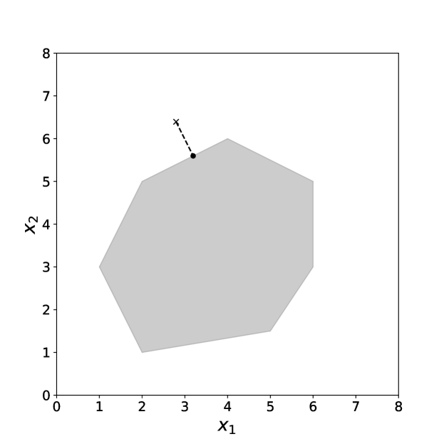
(a) Polytope

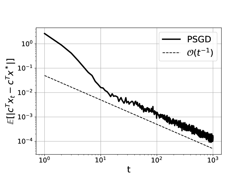
(b) Convergence for batch size $B=5$

Figure 3: Polytope of the two variables linear programming problem and convergence of projected stochastic gradient descent on the two variables linear programming example. In Figure 3(a), the shaded area is the bounded polytope and the cross is one of the points of iterations and the black point is the corresponding projection. In Figure 3(b), expectation is computed over 1000 realizations. The parameters of step size are chosen as $a=0.5,b=1$ and $\gamma=1$ such that $\alpha_{t}=0.5/(1+t)$. The costs $\bm{c}_{t}$ are computed with batch size $B=5$. The fitted slope is -1.07.

5.4 Probability Simplex

In this section, we consider a higher dimension for the optimization over the probability simplex as an example. There are simple efficient algorithms for projection onto the probability simplex (Duchi et al., 2008). The problem that we solve is formulated as follows

minimize $$\quad p_{1}\bar{c}_{1}+p_{2}\bar{c}_{2}+...+p_{n}\bar{c}_{n}=\bm{\bar{c}^{T}\bm{p}}\quad\text{subject to}\quad\sum_{i=1}^{n}p_{i}=1\quad\text{over}\quad p_{i}\geq 0,\ \forall i=1,...,n,$$

where $\bar{c}_{1}<\bar{c}_{2}<...<\bar{c}_{n}$ and $n=50$. We label the polytope due to the constraint as $\mathcal{P}$ and suppose that the cost vector $\mathbb{\bar{c}}$ is unknown but can be sampled from a normal distribution with a certain mean vector and covariance matrix. In particular, for $t\in\mathbb{Z}_{+}$, we apply the stochastic gradient descent iteration: $\bm{p}_{t+1}=\Pi_{\mathcal{P}}(\bm{p}_{t}-\alpha_{t}\bm{c_{t}}),$ where $\mathbb{c_{t}}\sim\mathcal{N}(\mathbb{\bar{c}},\mathbb{1})$ and $\alpha_{t}={a}/{t}$ with $a>0$. According to the special settings above, the minimum of this problem is $\bm{p}^{*}=(1,0,...,0)$. We expect that $\mathbb{E}\left[|\bm{\bar{c}^{T}\bm{p}_{t}}-\bm{\bar{c}^{T}}\bm{p}^{*}|\right]=O\left({1}/{t}\right).$ Figure 4(a) confirms that the projected stochastic gradient descent converges with an order of $-1$.

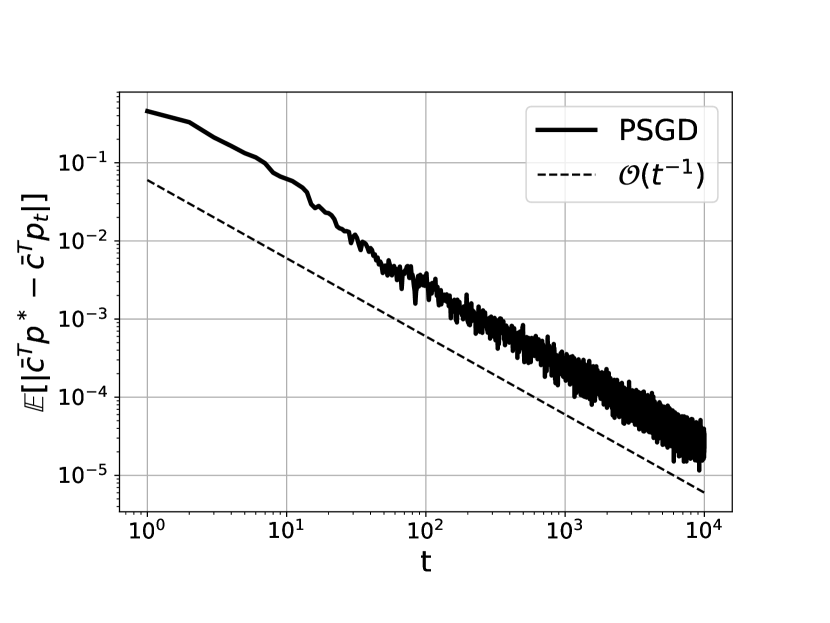
(a) Probability simplex example

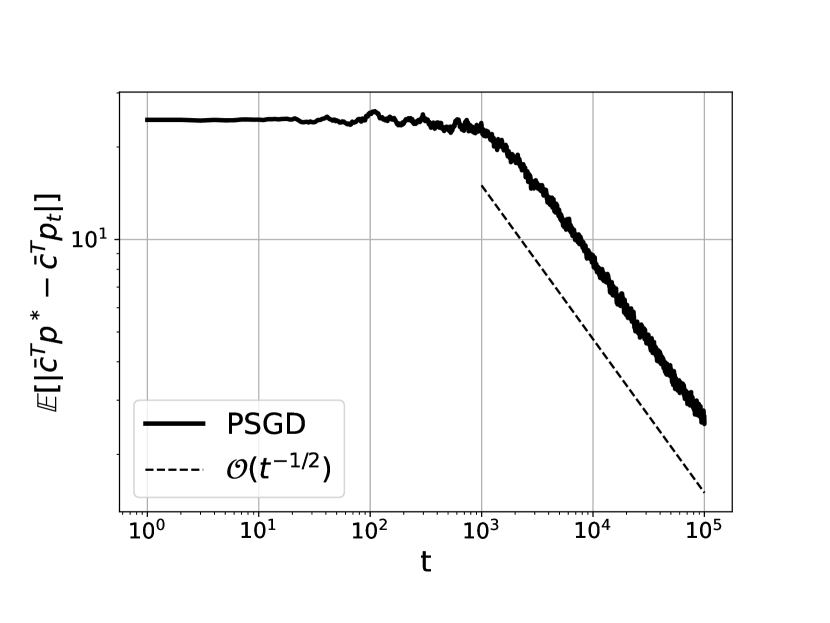
(b) Multi-arm bandit problem

Figure 4: Convergence of projected stochastic gradient descent on the probability simplex example and multi-arm bandit problem. Expectations are computed over 100 realizations and the parameter of step size is chosen as $a=1$ such that $\alpha_{t}=1/t$ for both. In Figure 4(a), the fitted slope is -1.014. In Figure 4(b), the fitted slope is -0.475.

Although it falls somewhat outside of the scope of the results in this paper. It is also possible to consider the multi-armed bandit variation of this problem. Here the natural generalization of the projected gradient descent algorithm applies importance sampling. Here we sample an index $i_{t}$ according to the distribution $\bm{p}_{t}$ and apply the updated $p_{i,t+1}=p_{i,t}-\alpha_{t}\frac{c_{i,t}}{p_{i,t}}\mathbb{I}[i=i_{t}]\,$ for $i=1,...,n$. Simulations suggest a rate of convergence of the order of $O(1/\sqrt{t})$, see Figure 4(b).

5.5 Three-state two-action Markov decision process

We now consider the first reinforcement learning application of our results. This is a relatively simple MDP which is described as follows. We consider a MDP with three states $\mathcal{S}=\{s_{1},s_{2},s_{3}\}$. In each state, there are two actions $\mathcal{A}=\{a_{1},a_{2}\}$, corresponding to move anticlockwise ($a_{1}$) and clockwise ($a_{2}$). Figure 5(a) shows the states and actions. When we choose to take an action, the probability of going to the desired state is $2/3$ otherwise one of the states uniformly at random. We assume that the costs $c(s,a)$ are independent normally distributed with $c(s_{i},a_{j})\sim N(i,1)$, for $i=1,2,3$. The states and actions are sampled according to the predetermined probability distribution $\bm{\pi}=(\pi(s,a)=1/6:s\in\mathcal{S},a\in\mathcal{A})$. Figure 5(b) demonstrates the correct rate of convergence as predicted.

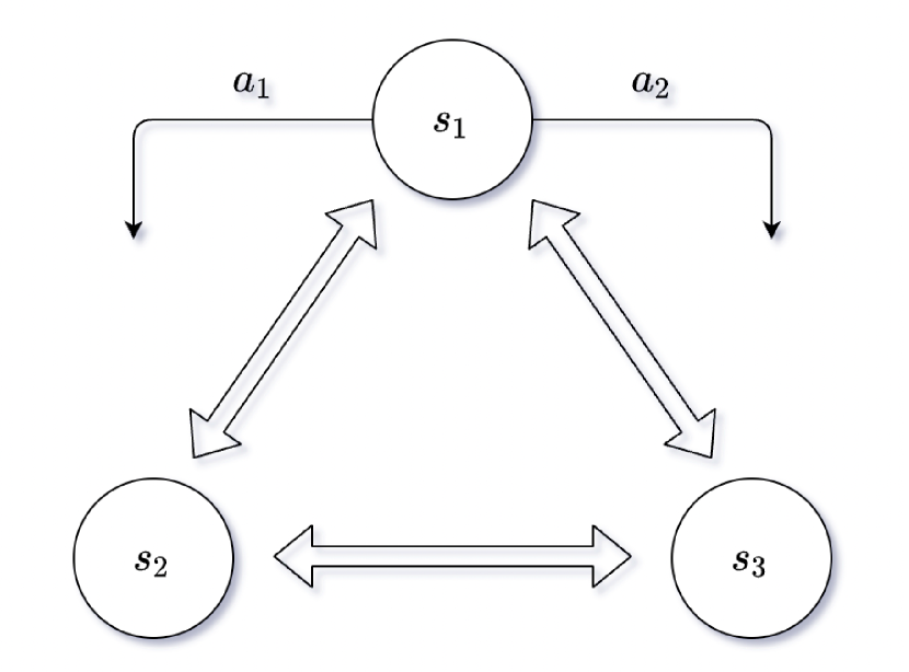
(a) Three-state two-action MDP graph

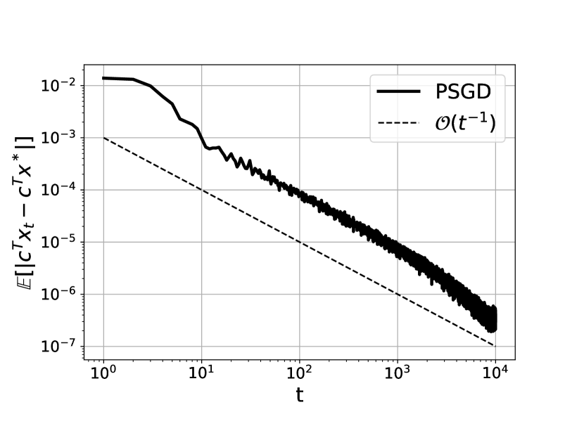
(b) Three-state two-action MDP example

Figure 5: The three-state two-action MDP graph and convergence of projected stochastic gradient descent on the three-state two-action MDP example. In Figure 5(b), the expectation is computed over 20 realizations. The costs $c_{t}(s,a)$ are computed with batch size $B=200$. The parameters of step size are chosen as $a=0.1,b=1$ and $\gamma=1$ such that $\alpha_{t}=0.1/(1+t)$. The fitted slope is -1.29.

5.6 Blackjack

We now consider a larger tabular reinforcement learning problem for the game of Blackjack. Blackjack is a simple card game where a player is initially dealt two cards. The player is dealt cards sequentially before deciding to stop. The player must attempt to reach a total that is more than the dealer but not more than 21. The problem is described in more detail in Sutton and Barto (2018). The states of the problem depend on three factors which are: the player’s current points (4–22); usable ace (with or without); dealer’s showing card (1–10), which gives 290 states in total.

We label the states in sequence starting with $s_{1}$ being no usable ace, the player’s current points 4 and dealer’s showing card 1, and ending with $s_{290}$ being usable ace, the player’s current points 21 and dealer’s showing card 10. The actions simply consist of hitting ($a_{1}$) and sticking ($a_{0}$). Denote the collection of states $\mathcal{S}=\{s_{i}:i=1,...,290\}$ and the collection of actions $\mathcal{A}=\{a_{i}:i=0,1\}$.

We assume that the reward $\bm{\bar{r}}=(\bar{r}(s,a):s\in\mathcal{S},a\in\mathcal{A})$ can be sampled for each iteration of the projected stochastic gradient descent by carrying on the following procedure. We first simulate IID samples $(s_{t}^{i},a_{t}^{i}),\ i=1,...,B$ from the distribution $\bm{\pi}=(\pi(s,a)=1/580:s\in\mathcal{A},a\in\mathcal{A})$ and then define the cost similar as Equation (27) with $\bar{c}(s_{t}^{i},a_{t}^{i})=-\bar{r}(s_{t}^{i},a_{t}^{i}).$ In addition, according to the rules, it is reasonable to set the discount factor $\beta=1$. Applying the PSGD with the learning rate of the form $\alpha_{t}=a/(b+t)^{\gamma}$, for $a,b>0$ and $\gamma\in[0,1]$, the projected stochastic gradient descent converges with a rate of $O(1/t^{\gamma})$ in expectation. The rate $O(1/t)$ with $\gamma=1$ is shown in Figure 6.

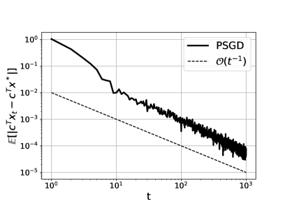
Figure 6: Convergence of projected stochastic gradient descent on the Blackjack example. The expectation is computed over 10 realizations. The costs $c_{t}(s,a)$ are computed with batch size $B=200$. The parameters of step size are chosen as $a=0.1,b=1$ and $\gamma=1$ such that $\alpha_{t}=0.1/(1+t)$. The fitted slope is -1.23.

6 Conclusions

Motivated by results on the exponential distributions found for stationary queueing networks in heavy traffic, we have established convergence rates for constrained stochastic approximation algorithms. Our results extend the findings on Markov chains by Hajek (1982) to stochastic approximation. These results prove exponential concentration bounds which differ from the normally distributed concentration bounds which typically occur for unconstrained stochastic approximation. Moreover, these results lead to faster convergence rates that differ from those predicted by standard stochastic approximation bounds.

Acknowledgement: We thank the reviewers for their help in improving this paper. We are particularly grateful to a referee for the reference, Davis et al. (2019), which lead to Theorem 3.

Appendix A Appendix to Theoretical Results

A.1 Lemma for Section 3.2

Lemma 5.

For projected stochastic gradient descent [cf. (5)], if for all $t\in\mathbb{Z}_{+}$ there exists $a,b>0$ such that

$$\mathbb{P}(||\bm{c}_{t}||\geq z|\mathcal{F}_{t})\leq ae^{-bz}$$ (28)

and $\nabla f(\bm{x})$ is continuous, then (C2) holds, that is

$$\Big{[}|f(\bm{x}_{t+1})-f(\bm{x}_{t})|\big{|}\mathcal{F}_{t}\Big{]}\leq\alpha_{t}Y\,,\quad\text{with}\quad\mathbb{E}[e^{\eta Y}]<\infty$$ (29)

for some $\eta>0$.

Proof.

(Proof of Lemma 5). Notice by Taylor’s Theorem, for some $\bm{y}_{t}$ belonging to the line segment between $\bm{x}_{t}$ and $\bm{x}_{t+1}$, it holds that

$$|f(\bm{x}_{t+1})-f(\bm{x}_{t})|= |(\bm{x}_{t+1}-\bm{x}_{t})\cdot\nabla f(\bm{y}_{t})|$$

$$\leq\, ||\bm{x}_{t+1}-\bm{x}_{t}||\cdot||\nabla f(\bm{y}_{t})||$$

$$\leq\, \alpha_{t}||\bm{c}_{t}||\max_{\bm{x}\in\mathcal{X}}||\nabla f(\bm{x})||\,.$$

Thus we can see that the moment generating function condition (29) holds if we can prove that

$$\mathbb{E}[e^{\eta||\bm{c}_{t}||}|\mathcal{F}_{t}]<\infty$$ (30)

for some $\eta>0$.

The condition (30) is a consequence of (28). Specifically,

$$\mathbb{E}[e^{\eta||\bm{c}_{t}||}|\mathcal{F}_{t}]= \int_{0}^{\infty}\mathbb{P}(e^{\eta||\bm{c}_{t}||}>y\,|\mathcal{F}_{t})dy$$

$$\leq\, 1+\int_{1}^{\infty}\mathbb{P}\Big{(}||\bm{c}_{t}||\geq\frac{1}{\eta}\log y\Big{|}\mathcal{F}_{t}\Big{)}dy$$

$$\leq\, 1+\int_{1}^{\infty}ay^{-b/\eta}dy<\infty\qquad\text{ for }0<\eta<b\,.$$ (31)

Thus from (31) we see that (30) holds and thus the required condition (29) holds. ∎

A.2 Technical Lemmas for the Proof of Proposition 1

See 1

Proof.

(Proof of Lemma 1). Applying the definition of $L_{t}$ and the drift Condition (C1) gives

$$\mathbb{E}[L_{t+1}-L_{t}|\mathcal{F}_{t}]= \,\mathbb{E}[f(\bm{x}_{t+1})-f(\bm{x}_{t})|\mathcal{F}_{t}]+(\alpha_{t}-\alpha_{t+1})B$$

$$\leq -2\alpha_{t}\kappa+(\alpha_{t}-\alpha_{t+1})B$$

$$\leq -2\alpha_{t}\kappa\left[1-(\alpha_{t}-\alpha_{t+1})B/\alpha_{t}\kappa\right]$$

Since $(\alpha_{t}-\alpha_{t+1})/\alpha_{t}\rightarrow 0$, there exists a constant $t_{0}$ such that $(\alpha_{t}-\alpha_{t+1})/\alpha_{t}<\kappa/2B$ for all $t\geq t_{0}$. This gives the first drift condition (11).

For the second condition, for $t\geq t_{0}$ with $t_{0}$ as just defined:

$$\big{[}|L_{t+1}-L_{t}|\big{|}\mathcal{F}_{t}\big{]}\leq \,\left[|f(\bm{x}_{t+1})-f(\bm{x}_{t})|\big{|}\mathcal{F}_{t}\right]+|\alpha_{t+1}-\alpha_{t}|B$$

$$\leq \,\alpha_{t}Y+\alpha_{t}\frac{(\alpha_{t}-\alpha_{t+1})}{\alpha_{t}}B$$

$$\leq \,\alpha_{t}(Y+\kappa/2)\,.$$

Taking $Z=Y+\kappa/2$, it is clear that condition (12) holds for $Z$ as an immediate consequence of the boundedness condition on $Y$ in (C2). ∎

See 3

Proof.

(Proof of Lemma 3). It is straight-forward to show that for $a,a^{\prime},A,A^{\prime}>0$

$$\frac{a}{a^{\prime}}\leq\frac{A}{A^{\prime}}\quad\text{if and only if}\quad\frac{a+A}{a^{\prime}+A^{\prime}}\leq\frac{A}{A^{\prime}}\,.$$ (32)

[Note that both expression above are equivalent to $AA^{\prime}+aA^{\prime}\leq AA^{\prime}+a^{\prime}A$.]

Take positive numbers $a_{s},a_{s}^{\prime},\ s=1,...,t$. If

$$\frac{a_{s}}{a_{s}^{\prime}}\leq\frac{a_{k}}{a_{k}^{\prime}}$$

for $k=s-1,...,t$, then

$$\sum_{k=s-1}^{t}a_{k}^{\prime}a_{s}\leq\sum_{k=s-1}^{t}a_{k}a_{s}^{\prime}.$$ (33)

Thus,

$$\frac{a_{s}}{a_{s}^{\prime}}\leq\frac{\sum_{k=s-1}^{t}a_{k}}{\sum_{k=s-1}^{t}a_{k}^{\prime}}.$$

Thus applying (32) with $A=\sum_{k=s-1}^{t}a_{k}$ and $A^{\prime}=\sum_{k=s-1}^{t}a_{k}^{\prime}$ gives

$$\frac{\sum_{k=s}^{t}a_{k}}{\sum_{k=s}^{t}a_{k}^{\prime}}\leq\frac{\sum_{k=s-1}^{t}a_{k}}{\sum_{k=s-1}^{t}a_{k}^{\prime}}.$$ (34)

Finally, taking $a_{k}=\alpha_{k}$ and $a_{k}^{\prime}=\alpha_{k}^{2}$, we see that (33) holds since $\alpha_{t}$ is decreasing. Thus, from (34), we see that the result (15) holds.

If the condition (7) holds then $\liminf_{t\rightarrow\infty}\alpha_{2t}/\alpha_{t}>0$ implies

$$\frac{\alpha_{t}}{\alpha_{\lfloor t/2\rfloor}}>\sqrt{G}$$ (35)

for some $G>0$. Since the sequence is decreasing and (35) holds, we have that

$$\frac{\sum_{k=\lfloor t/2^{n}\rfloor}^{t}\alpha_{k}}{\sum_{k=\lfloor t/2^{n}\rfloor}^{t}\alpha_{k}^{2}}\geq\frac{(t-\lfloor t/2^{n}\rfloor)\alpha_{t}}{(t-\lfloor t/2^{n}\rfloor)\alpha_{\lfloor t/2^{n}\rfloor}^{2}}=\frac{\alpha^{2}_{t}}{\alpha^{2}_{\lfloor t/2^{n}\rfloor}}\frac{1}{\alpha_{t}}=\frac{\alpha^{2}_{t}}{\alpha^{2}_{\lfloor t/2\rfloor}}\times...\times\frac{\alpha^{2}_{\lfloor t/2^{n-1}\rfloor}}{\alpha^{2}_{\lfloor t/2^{n}\rfloor}}\frac{1}{\alpha_{t}}\geq\frac{G^{n}}{\alpha_{t}}\,.$$

Applying this to (15) with $t_{1}=\lfloor t/2^{n}\rfloor$ gives

$$\min_{s=\lfloor t/2^{n}\rfloor,...,t}\left\{\frac{\sum_{k=s}^{t}\alpha_{k}}{\sum_{k=s}^{t}\alpha_{k}^{2}}\right\}\geq\frac{G^{n}}{\alpha_{t}}\,.$$

Thus (16) holds as required. ∎

A.3 Proof of Theorem 1 for $\gamma=1$

Proof.

(Proof of Theorem 1 for $\gamma=1$). Now suppose that $\gamma=1$ then the analogous bound to (21) is

$$\sum_{s=\lfloor(v-u)/2^{n}\rfloor}^{v-u}\alpha_{s}= \sum_{s=\lfloor(v-u)/2^{n}\rfloor}^{v-u}\frac{a}{(u+t)}\geq\,\int_{v/2^{n}-u}^{v-u}\frac{a}{(u+t)}ds={a}\left[\log(u+t)\right]^{v-u}_{v/2^{n}-u}=an\log 2\,.$$

We see that if we chose $n$ such that $n=\left\lceil\frac{(\alpha_{0}B+F)}{a\log 2}\right\rceil$ then $\sum^{t}_{s=\lfloor t/2^{n}\rfloor}\alpha_{s}\frac{\kappa}{2}\geq\alpha_{0}B+F\,,$ holds. Thus is we choose $n$ as above and $t_{0}=1$ then, again applying (8) from Proposition 1, we have the bound

$$\mathbb{P}(f(\bm{x}_{t+1})-f(\bm{x}^{\star})\geq z)\leq(1+H){e^{-\frac{\kappa G^{n}}{2E\alpha_{t}}(z-\alpha_{t}B)}}\,.$$

Thus we see that the bound (2) holds with $I:=H+1$ and $J:={\kappa G^{n}}/{2E}$. Integrating the above bound then gives

$$\mathbb{E}[f(\bm{x}_{t+1})-f(\bm{x}^{\star})]\leq\left[\frac{2E(1+H)}{\kappa G^{n}}+B\right]\alpha_{t}\,.$$

Thus we see that (3) holds with $K:=B+{2E(1+H)}/{\kappa G^{n}}$. ∎

A.4 Technical Lemma for Linear Programming

See 4

The proof of Lemma 4 requires some careful bounding between optimal solutions and sub-optimal extreme points. The proof is given below. The result bounds the angle between optimal and sub-optimal points for a polytope.

Proof.

(Proof of Lemma 4). We assume without loss of generality that $\bar{\bm{c}}^{\top}\bm{x}^{\star}=0$ and $||\bar{\bm{c}}||=1$. Let $\mathcal{E}$ be the extreme points of $\mathcal{X}$. Let $\mathcal{E}^{\star}$ be the extreme points in $\mathcal{X}^{\star}$. Then let $\mathcal{E}^{\prime}:=\mathcal{E}\setminus\mathcal{E}^{\star}$ and $\mathcal{X}^{\prime}$ is the convex closure of $\mathcal{E}^{\prime}$. Let $a:=\min_{\bm{x}\in\mathcal{X}^{\prime}}\bar{\bm{c}}^{\top}\bm{x}$ and $D:=\max_{\bm{x}^{\star}\in\mathcal{X}^{\star},\bm{x}^{\prime}\in\mathcal{X}^{\prime}}||\bm{x}^{\star}-\bm{x}^{\prime}||.$ We will show we can take $K:={a}/{D}$.

For all $\bm{x}\in\mathcal{X}\setminus\mathcal{X}^{\star}$, $\bm{x}$ must be a convex combination of a point in $\mathcal{X}^{\star}$ and a point in $\mathcal{X}^{\prime}.$ Specifically,

$$\bm{x}=(1-p)\bm{x}_{0}+p\bm{x}_{1},$$ (36)

for $\bm{x}_{0}\in\mathcal{X}^{\star}$ and $\bm{x}_{1}\in\mathcal{X}^{\prime}$ and $p\in(0,1]$. Then, as required,

$$\frac{\bar{\bm{c}}^{\top}\bm{x}}{||\bm{x}-\bm{x}^{\star}||}\geq\frac{\bar{\bm{c}}^{\top}(\bm{x}-\bm{x}_{0})}{||\bm{x}-\bm{x}_{0}||}=\frac{\bar{\bm{c}}^{\top}(\bm{x}_{1}-\bm{x}_{0})}{||\bm{x}_{1}-\bm{x}_{0}||}\geq\frac{a}{D}=K>0\,.$$

The first inequality above uses the fact that $\bm{x}^{\star}$ is closest to $\bm{x}$. The equality applies (36). Then finally, we apply the definitions of $a$, $D$ and $K$. ∎

Appendix B Appendix to Simulations

B.1 LP formulation

The linear program considered in Section 5.3 is:

Minimize $$4x_{1}+6x_{2} =\bm{\bar{c}}^{T}\bm{x}$$

subject to $$1.5x_{1}-x_{2} \leq 6$$

$$-x_{1}+2x_{2} \leq 8$$

$$-2x_{1}+x_{2} \leq 1$$

$$-2x_{1}-x_{2} \leq-5$$

$$x_{1}-6x_{2} \leq-4$$

$$x_{1}+2x_{2} \leq 16$$

$$x_{1} \leq 6,$$

over $$x_{1},x_{2}\in\mathbb{R}$$

In the projected stochastic gradient descent steps, the cost vectors are sampled from a joint Gaussian distribution of independent random variables with mean vector $\bm{\bar{c}}.$

References

- Asmussen [2003] Asmussen, S. (2003). Applied probability and queues, volume 2. Springer.
- Bertsekas [2015] Bertsekas, D. (2015). Convex optimization algorithms. Athena Scientific, Belmont, MA.
- Bertsimas et al. [2001] Bertsimas, D., Gamarnik, D., and Tsitsiklis, J. N. (2001). Performance of multiclass markovian queueing networks via piecewise linear lyapunov functions. Annals of Applied Probability, pages 1384–1428.
- Birge and Louveaux [2011] Birge, J. R. and Louveaux, F. (2011). Introduction to stochastic programming. Springer Science & Business Media, New York.
- Bottou et al. [2018] Bottou, L., Curtis, F. E., and Nocedal, J. (2018). Optimization methods for large-scale machine learning. Siam Review, 60(2):223–311.
- Buche and Kushner [2002] Buche, R. and Kushner, H. J. (2002). Rate of convergence for constrained stochastic approximation algorithms. SIAM journal on control and optimization, 40(4):1011–1041.
- Chen et al. [2022] Chen, Z., Mou, S., and Maguluri, S. T. (2022). Stationary behavior of constant stepsize SGD type algorithms: An asymptotic characterization. Proceedings of the ACM on Measurement and Analysis of Computing Systems, 6(1):1–24.
- Davis and Drusvyatskiy [2019] Davis, D. and Drusvyatskiy, D. (2019). Stochastic model-based minimization of weakly convex functions. SIAM Journal on Optimization, 29(1):207–239.
- Davis et al. [2019] Davis, D., Drusvyatskiy, D., and Charisopoulos, V. (2019). Stochastic algorithms with geometric step decay converge linearly on sharp functions. arXiv preprint arXiv:1907.09547.
- Duchi et al. [2008] Duchi, J., Shalev-Shwartz, S., Singer, Y., and Chandra, T. (2008). Efficient projections onto the l 1-ball for learning in high dimensions. In Proceedings of the 25th international conference on Machine learning, pages 272–279.
- Duchi and Ruan [2021] Duchi, J. C. and Ruan, F. (2021). Asymptotic optimality in stochastic optimization.
- Fabian [1968] Fabian, V. (1968). On asymptotic normality in stochastic approximation. The Annals of Mathematical Statistics, pages 1327–1332.
- Hajek [1982] Hajek, B. (1982). Hitting-time and occupation-time bounds implied by drift analysis with applications. Advances in Applied probability, 14(3):502–525.
- Harrison and Williams [1987] Harrison, J. M. and Williams, R. J. (1987). Multidimensional reflected brownian motions having exponential stationary distributions. The Annals of Probability, pages 115–137.
- Hazan et al. [2016] Hazan, E. et al. (2016). Introduction to online convex optimization. Foundations and Trends® in Optimization, 2(3-4):157–325.
- Kingman [1964] Kingman, J. F. (1964). A martingale inequality in the theory of queues. In Mathematical Proceedings of the Cambridge Philosophical Society, volume 60, pages 359–361. Cambridge University Press.
- Kushner and Clark [1978] Kushner, H. and Clark, D. (1978). Stochastic Approximation Methods for Constrained and Unconstrained Systems. Applied Mathematical Sciences. Springer New York, New York.
- Kushner and Yin [2003] Kushner, H. and Yin, G. (2003). Stochastic Approximation and Recursive Algorithms and Applications. Stochastic Modelling and Applied Probability. Springer New York, New York.
- Meyn and Tweedie [2012] Meyn, S. P. and Tweedie, R. L. (2012). Markov chains and stochastic stability. Springer Science & Business Media, London.
- Michelot [1986] Michelot, C. (1986). A finite algorithm for finding the projection of a point onto the canonical simplex of . Journal of Optimization Theory and Applications, 50:195–200.
- Moulines and Bach [2011] Moulines, E. and Bach, F. (2011). Non-asymptotic analysis of stochastic approximation algorithms for machine learning. Advances in neural information processing systems, 24.
- Nemirovski et al. [2009] Nemirovski, A., Juditsky, A., Lan, G., and Shapiro, A. (2009). Robust stochastic approximation approach to stochastic programming. SIAM Journal on optimization, 19(4):1574–1609.
- Robbins and Siegmund [1971] Robbins, H. and Siegmund, D. (1971). A convergence theorem for non negative almost supermartingales and some applications. In Optimizing methods in statistics, pages 233–257. Elsevier.
- Schweitzer and Seidmann [1985] Schweitzer, P. J. and Seidmann, A. (1985). Generalized polynomial approximations in markovian decision processes. Journal of mathematical analysis and applications, 110(2):568–582.
- Shapiro et al. [2021] Shapiro, A., Dentcheva, D., and Ruszczynski, A. (2021). Lectures on stochastic programming: modeling and theory. SIAM, Philadelphia, PA.
- Sutton and Barto [2018] Sutton, R. S. and Barto, A. G. (2018). Reinforcement learning: An introduction. MIT press, Cambridge, Massachusetts, London, England.