Distributional Correlation–Aware Knowledge Distillation for Stock Trading Volume Prediction

Abstract

Traditional knowledge distillation in classification problems transfers the knowledge via class correlations in the soft label produced by teacher models, which are not available in regression problems like stock trading volume prediction. To remedy this, we present a novel distillation framework for training a light-weight student model to perform trading volume prediction given historical transaction data. Specifically, we turn the regression model into a probabilistic forecasting model, by training models to predict a Gaussian distribution to which the trading volume belongs. The student model can thus learn from the teacher at a more informative distributional level, by matching its predicted distributions to that of the teacher. Two correlational distillation objectives are further introduced to encourage the student to produce consistent pair-wise relationships with the teacher model. We evaluate the framework on a real-world stock volume dataset with two different time window settings. Experiments demonstrate that our framework is superior to strong baseline models, compressing the model size by $5\times$ while maintaining $99.6\%$ prediction accuracy. The extensive analysis further reveals that our framework is more effective than vanilla distillation methods under low-resource scenarios.

1 Introduction

Large deep neural networks (DNNs) like Transformer [30] have achieved superior performance in various areas like computer vision [6], natural language processing [5] and time series forecasting problems like stock trading volume prediction [32]. However, the increase of model parameters demands more computational resources, limiting their applicability in latency-sensitive scenarios like high-frequency trading (HFT). The pursuit of a better performance-efficiency trade-off promotes an active research field toward compressing large DNNs while maintaining promising model performance. Pilot model compression techniques include pruning [8], quantization [11, 28] and knowledge distillation [9, 24]. Pruning improves the parameter efficiency by de-activating redundant structures in the network, and quantization focuses on exploring fewer bits for representing the model weights. While effective in reducing the model size, these two methods require hardware-specific support for actually gaining the speed-up. On the other hand, knowledge distillation (KD), trains a much smaller student model by utilizing the learned knowledge from a large teacher model. It has been prove successful in various classifications problems like natural language understanding [26, 29] and image classification [9, 24], and recent studies have demonstrated that KD can obtain a compact student model that matches or even outperforms the teacher model [24, 7, 13].

Traditional knowledge distillation works relatively well for classification problems, as it can transfer the dark knowledge, i.e., the softened logits of the teacher prediction, to the student. The softened logits contain richer supervision signals than the vanilla one-hot class label, reflecting the semantic correlation between different classes and thus boosting student performance. However, this advantage cannot hold in regression problems like stock trading volume prediction, as the teacher model only produces real-valued predictions which have an identical characteristic to the oracle label. Without an optimal carrier for the learned knowledge in the teacher, the effects of KD are limited in regression problems.

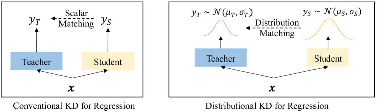
Figure 1: Distributional knowledge distillation for regression problems. While conventional KD for regression problems only transfers the knowledge by matching the scalar $y_{S}$ to $y_{T}$, our proposed distributional KD operates on the distributional level and provides more informative supervision for the student.

To remedy this, in this paper, we propose a distributional knowledge distillation framework for regression problems, as illustrated in Figure 1. Specifically, we first turn the problem into a probabilistic forecasting problem. We cast the trading volume prediction problem as a conditional probability distribution modeling problem given the historical data. The teacher and the student are both probabilistic forecasting models trained by minimizing the log-likelihood of the training data. The learned knowledge from the teacher model is then transferred to the student by minimizing the discrepancy between the predicted distributions. Besides, recent studies have shown that the capacity gap between the teacher model and the student model may harm the distillation effect [21, 15], which is also observed in our vanilla distributional KD framework. To alleviate this, we design two correlations between different samples regarding the output distributions. The student is then trained to predict pair-wise correlations consistently with the teacher model, by incorporating the correlation congruence objectives into the distillation process. These objectives serve as auxiliary objectives to provide more informative supervision for alleviating the capacity gap problem. We validate our proposal by distilling a multiple-layer Transformer model into a single layer student model. Experiments on a real-world stock volume prediction dataset show that our framework can reduce the number of model parameters by $5$ times while maintaining $99.6\%$ prediction accuracy. Further analysis shows that our framework is more effective under low-resource settings and can make the student produce more calibrated predictions.

2 Methodology

In this section, we first formulate the stock trading volume prediction problem and introduce the metrics defined for evaluation. Followingly, we introduce conventional knowledge distillation for classification problems. We then elaborate the proposed distributional correlation-aware knowledge distillation framework for the regression problem.

2.1 Task Formulation

Stock trading volume prediction aims at predicting the market trading volume given historical transaction data. Specifically, given training dataset consists of $N$ data samples $\mathcal{D}=\{(\mathbf{x}_{1},y_{1}),\ldots,(\mathbf{x}_{N},y_{N})\}$, where $\mathbf{x}_{i}$ denotes the transaction data including open, closing, lowest, highest price and the trading volume in the past time windows, and $y_{i}$ is the target volume of the $i$-th sample. Our goal is training a light-weight student model $S$, to predict the trading volume $\hat{y}$, by learning from a larger teacher model $T$. The student performance is measured by the mean squared error (MSE), mean absolute error (MAE) and prediction accuracy (ACC):

$$\mathrm{MSE} =\mathbb{E}_{(\mathbf{x},y)\sim\mathcal{D}}(\hat{y}-y)^{2},$$ (1)

$$\mathrm{MAE} =\mathbb{E}_{(\mathbf{x},y)\sim\mathcal{D}}|\hat{y}-y|,$$

$$\mathrm{ACC} =\mathbb{P}_{(\mathbf{x},y)\sim\mathcal{D}}\left(\left(\hat{y}-y_{\text{last }}\right)\times\left(y-y_{\text{last }}\right)>0\right),$$

where $y_{\text{last}}$ is the volume of the most last time slot. Thus, ACC is the accuracy of whether the volume increases or decreases compared to the last time slot.

2.2 Conventional Knowledge Distillation for Classification

Knowledge distillation is a classic framework for transferring the knowledge of a larger teacher model to a light-weight student model. The main idea behind is training the student model to mimic the outputs of the teacher model. Specifically, in a classification problem, given the one-hot label $\mathbf{y}$, the student prediction $\mathbf{O}_{S}$ and the teacher prediction $\mathbf{O}_{T}$ over the class set, KD is usually achieved by minimizing both the hard label error and a soft label error between the student and the teacher predictions:

$$\mathcal{L}_{KD}=\alpha\mathcal{H}\left(\mathbf{y},\mathbf{O}_{S}\right)+(1-\alpha)\mathcal{H}\left(\mathbf{O}_{T},\mathbf{O}_{S}\right),$$ (2)

where $\mathcal{H}(\cdot,\cdot)$ denotes the cross-entropy objective and $\alpha$ is a tuning parameter controlling the relative contribution of cross-entropies. As $\mathbf{O}_{T}$ usually contains rich information regarding the semantic relationships between classes, the student can capture more fine-grained structured information from the teacher predictions than directly learning from the ground-truth label. However, this characteristic cannot hold in regression problems like stock trading volume prediction, as the teacher predictions are also real-valued scalars. The predicted scalars of the teacher cannot convey more information to benefit the student, motivating us to explore a better distillation framework for regression problems.

2.3 Distributional Knowledge Distillation for Regression Problems

To facilitate the distillation effect, we propose to cast the trading volume prediction problem as a probabilistic forecasting problem, thus the information can be transferred at the distribution level. Specifically, following DeepAR [25], instead of directly predicting the scalar, we assume that the predicted trading volume follows a Gaussian distribution $\mathcal{N}(\mu,\sigma)$, turning the regression problem into a likelihood model as:

$$p(y\mid\mu,\sigma) =\frac{1}{\sqrt{2\pi\sigma^{2}}}\exp\left(-\frac{(y-\mu)^{2}}{2\sigma^{2}}\right).$$ (3)

The Gaussian distribution is parameterized by a mean $\mu$ and a standard deviation $\sigma$, which can be obtained by applying affine transformations on the model encoding $\mathbf{h}$ of the input transaction data $\mathbf{x}$:

$$\mu\left(\mathbf{h}\right) =\mathbf{w}_{\mu}^{T}\mathbf{h}+b_{\mu}$$ (4)

$$\sigma\left(\mathbf{h}\right) =\log\left(1+\exp\left(\mathbf{w}_{\sigma}^{T}\mathbf{h}+b_{\sigma}\right)\right),$$

where $\mathbf{w}_{\mu}$, $b_{\mu}$, $\mathbf{w}_{\sigma}$ and $b_{\sigma}$ are learnable parameters of the affine transformation. Note that the standard deviation is wrapped with a softplus activation to ensure the value is positive. With this formulation, a model $M$ can be trained by minimizing the negative log-likelihood of the ground-truth data:

$$\mathbf{h}_{i} =M(\mathbf{x}_{i})$$ (5)

$$\mathcal{L}_{\text{NLL}} =-\sum_{i=1}^{N}\log p\left(y_{i}\mid\mu\left(\mathbf{h}_{i}\right),\sigma\left(\mathbf{h}_{i}\right)\right).$$

We first train a teacher model with the above objective, and then transfer the learned knowledge into the student model by minimizing the Kullback-Leibler (KL) divergence between the Gaussian distributions [22] predicted by the teacher and the student model:

$$\mathcal{L}_{\text{DKD}} =-\sum_{i}^{N}\text{KL}\left(\mathcal{N}\left(\mu^{T}_{i},\sigma^{T}_{i}\right)\|\mathcal{N}\left(\mu^{S}_{i},\sigma^{S}_{i}\right)\right)$$ (6)

$$=-\sum_{i}^{N}\left(\log\frac{\sigma^{S}_{i}}{\sigma^{T}_{i}}+\frac{\left(\sigma^{T}_{i}\right)^{2}+\left(\mu^{T}_{i}-\mu^{S}_{i}\right)^{2}}{2\left(\sigma^{S}_{i}\right)^{2}}-\frac{1}{2}\right),$$

where $\mu^{S}_{i}$, $\mu^{T}_{i}$, $\sigma^{S}_{i}$ and $\sigma^{T}_{i}$ are the mean and standard deviation outputs of the student model and the teacher model of the $i$-th data sample, respectively.

2.4 Transferring Knowledge via Correlation Consistency

Directly minimizing the KL-divergence between distributions can be challenging for the student model, as revealed by recent studies regarding the capacity gap between the teacher model and the student model [21, 15]. To remedy this, we introduce correlational knowledge distillation objectives which capture the pair-wise relationships between the examples for alleviating this issue. Specifically, given the outputs distributions of the teacher models and the students model on $m$ data samples:

$$\boldsymbol{N}_{T} =\left[\mathcal{N}_{1}^{T},\ldots,\mathcal{N}_{m}^{T}\right]$$ (7)

$$\boldsymbol{N}_{S} =\left[\mathcal{N}_{1}^{S},\ldots,\mathcal{N}_{m}^{S}\right].$$

A mapping function $\psi$ is introduced for mapping the outputs to a pairwise correlation matrix $\boldsymbol{C}$:

$$\psi:\boldsymbol{N}\rightarrow\boldsymbol{C}\in\mathbb{R}^{m\times m}.$$ (8)

The element in $\boldsymbol{C}$ denotes the correlation between distributions on two sample $\mathbf{x}_{i}$ and $\mathbf{x}_{j}$:

$$\boldsymbol{C}_{ij}=\varphi\left(\mathcal{N}_{i},\mathcal{N}_{j}\right),\quad\boldsymbol{C}_{ij}\in\mathbb{R}.$$ (9)

The function $\varphi$ denotes a correlation metric that captures the relationship between two Gaussian distributions, and the two options we designed for the function will be elaborated later. The correlational knowledge in the teacher then can be transferred by training student to minimize the congruence objective:

$$\mathcal{L}_{\text{DCKD}} =\frac{1}{m^{2}}\left\|\psi\left(\boldsymbol{N}_{S}\right)-\psi\left(\boldsymbol{N}_{T}\right)\right\|_{2}^{2}$$ (10)

$$=\frac{1}{m^{2}}\sum_{i,j}\left(\varphi\left(\mathcal{N}_{i}^{S},\mathcal{N}_{j}^{S}\right)-\varphi\left(\mathcal{N}_{i}^{T},\mathcal{N}_{j}^{T}\right)\right)^{2}.$$

In this way, the student can learn to predict the correlation between instances consistently with the teacher model. The correlational distillation objective serves as an auxiliary objective. The student can first learn the correlations between its own predictions according to the teacher predictions, then make efforts towards predicting exactly the same as the teacher model. Followingly, we introduce two correlation metrics regarding the distance-wise and the angle-wise similarity between samples.

2.4.1 Distance-wise Correlation

Given two Gaussian distributions, a straightforward correlation metric is the distance between these two distributions. Specifically, we adopt the Jeffreys divergence (JSD) as the distance between $\mathcal{N}_{i}(\mu_{i},\sigma_{i})$ and $\mathcal{N}_{j}(\mu_{j},\sigma_{j})$ since it is symmetrized:

$$\varphi_{\text{Dist}}(\mathcal{N}_{i},\mathcal{N}_{j}) =\frac{1}{2}\left(\text{KL}\left(\mathcal{N}_{i}\|\mathcal{N}_{j}\right)+\text{KL}\left(\mathcal{N}_{j}\|\mathcal{N}_{i}\right)\right)$$ (11)

$$=\frac{1}{2}\left(\frac{1}{\sigma_{i}^{2}}+\frac{1}{\sigma_{j}^{2}}\right)\left(\left(\sigma_{i}-\sigma_{j}\right)^{2}+\left(\mu_{i}-\mu_{j}\right)^{2}\right).$$

We note that the JSD can be replaced with alternative distance measurements like Wasserstein distance. As our goal is developing a distributional distillation framework for regression problems and the JSD works well in practice, we leave the explorations on the choices of distance metrics for future work.

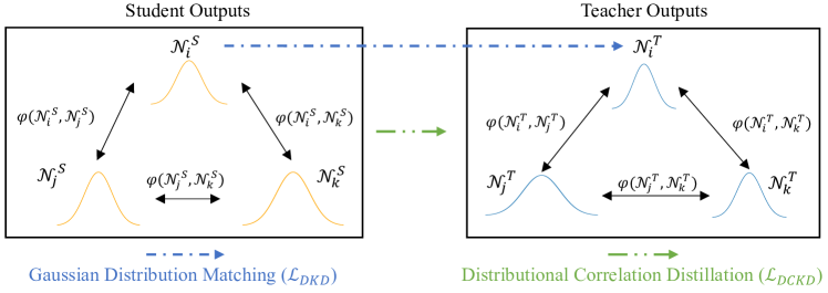
Figure 2: The main idea illustration of the proposed distributional correlation-aware distillation, which transfers the knowledge in the teacher model by matching the predicted Gaussian distributions, with correlational consistency distillation objectives for improving the student performance.

2.4.2 Angle-wise Correlation

Another commonly adopted similarity measurement is the angle-wise correlation, which is a higher-order relationship than the vanilla distance metric and thus can be more effective for transferring information [23]. In the Euclidean space, cosine similarity is a commonly adopted for evaluating the angle-wise correlation between two vectors:

$$\cos\langle\mathbf{u},\mathbf{v}\rangle=\frac{(\mathbf{u},\mathbf{v})}{\sqrt{(\mathbf{u},\mathbf{u})(\mathbf{v},\mathbf{v})}},$$ (12)

where $\left(\mathbf{u},\mathbf{v}\right)$ denotes the inner-product in the Euclidean space of two vectors. We extend this idea to Gaussian distributions and design a corresponding angle-wise cosine similarity metric for probabilistic distributions. Specifically, we define $(\mathcal{N}_{i},\mathcal{N}_{j})$ as the inner-product in the Hilbert space:

$$(\mathcal{N}_{i},\mathcal{N}_{j})=\int_{-\infty}^{+\infty}\mathcal{N}_{i}(t\mid\mu_{i},\sigma_{i})\mathcal{N}_{j}(t\mid\mu_{j},\sigma_{j})dt\ .$$ (13)

The cosine similarity thus can be calculated as:

$$\varphi_{\text{Cosine}}\left(\mathcal{N}_{i},\mathcal{N}_{j}\right)=\frac{(\mathcal{N}_{i},\mathcal{N}_{j})}{\sqrt{(\mathcal{N}_{i},\mathcal{N}_{i})(\mathcal{N}_{j},\mathcal{N}_{j})}}=\sqrt{\frac{2\sigma_{i}\sigma_{j}}{{\sigma_{i}^{2}+\sigma_{j}^{2}}}}\exp\left(-\frac{\left(\mu_{i}-\mu_{j}\right)^{2}}{2\left(\sigma_{i}^{2}+\sigma_{j}^{2}\right)}\right).$$ (14)

We refer readers to Appendix 0.A for the detailed proof of the inner-dot and the cosine similarity of Gaussian distributions.

By combining the correlation metrics with the distillation objective, the student model finally is trained by minimizing the following loss function:

$$\mathcal{L}=\lambda_{\text{NLL}}\mathcal{L}_{\text{NLL}}+\lambda_{\text{DKD}}\mathcal{L}_{\text{DKD}}+\lambda_{\text{Dist}}\mathcal{L}_{\text{Dist-CKD}}+\lambda_{\text{Cosine}}\mathcal{L}_{\text{Cosine-CKD}},$$ (15)

where $\lambda_{\text{NLL}}$, $\lambda_{\text{DKD}}$, $\lambda_{\text{Dist}}$ and $\lambda_{\text{Cosine}}$ are hyper-parameters for tuning the relative contribution of the proposed correlational distillation objectives. We name the methods that setting $\lambda_{\text{Dist}}=0$ and $\lambda_{\text{Cosine}}=0$ as Cosine-CKD and Dist-CKD, respectively. Figure 2 gives an overview of our proposed framework.

3 Experiments

In this section, we conduct experiments on a real-world stock trading volume prediction dataset for evaluating the effectiveness of our framework. We first introduce the dataset used for evaluation, followed by the details of compared baseline models and implementation details for reproducible results. Finally, we present the main results compared with strong baseline models.

Table 1: The statistics of the TPX500 datasets used in our paper. The training and validation datasets have no time window overlapping with the test dataset to avoid potential data leakage.

Dataset	Hourly			Daily
Split	Training	Validation	Test	Training	Validation	Test
# of Samples	49,712	16,571	26,841	81,950	27,317	38,316

3.1 Datasets

We conduct our experiments by collecting trading data from the largest $500$ stock names traded at Tokyo Exchange known as TPX500. For our research, we construct two datasets with different time windows, i.e., an hourly intra-day trading volume prediction dataset and a daily trading volume prediction dataset. The two datasets are both extracted from the price and trading volume data of the TPX500 between Jan. 2017 and June. 2018. Each data sample consists of the open, closing, lowest, highest price and trading volume in the past time windows and a target trading volume. We adopt the data of 2017 as the training set and development set, and the samples between Jan. 2018 and Jun. 2018 are adopted as the test set, making sure that the test set and the training dataset are non-overlapping. The dataset statistics can be found in Table 1.

3.2 Baselines

We compare our methods to the following baseline models, including:

Moving average methods, which adopts the averaged last 20-day transaction data as the predictions. We implement (1) Simple Moving Average (SMA), where the predictions are the averaged trading volume of the last $20$ days at the same time slot, i.e., $\hat{x}=\frac{1}{T}\sum_{i=1}^{T}x_{i}$, and (2) Exponential Moving Average (EMA), which pays more attention to the nearest values, by setting $y_{1}=x_{1}$ and $y_{t}=\rho x_{t}+(1-\rho)y_{t-1}$. $y_{T}$ is adopted as the prediction. We set $\rho=0.04$ following [32].

Teacher-free methods, which requires no teacher model for training the student. We implement two methods: (1) Min-MSE, where the student minimizes the mean-square error between the prediction and the ground-truth volume, and (2) DeepAR [25], which models the prediction as a conditional probability distribution and maximizes the log-likelihood of the oracle data.

Distillation methods, which utilizes the teacher model for enhancing the student model. Specifically, we implement (1) Vanilla KD [9], where the mean-square error of the student predictions and teacher predictions and the objective of the Min-MSE method are both optimized, similar to the original knowledge distillation in the classification problem, and (2) Attentive Imitation Loss (AIL) [27], where the supervision from imitating the teacher prediction is adaptively adjusted according to the relative correctness of the teacher model.

3.3 Implementation Details

Without loss of generality, we adopt the Transformer [30] model as the backbone model due to its powerful modeling ability. The teacher model consists of $6$ Transformer layer, which contains a self-attention module and a feed-forward network layer. We omit the description of the Transformer layer due to the space limit and refer readers to the original Transformer paper [30] for details. The student is a much smaller Transformer model with only one layer. The number of input, number of hidden units and the output dimension are all set to $200$, and the hidden states are split into $8$ heads for capturing sub-space relations. The teacher and the student only differ from the layer number. The resulting numbers of model parameters of the student and the teacher model are $0.3$M and $1.5$M, respectively. To eliminate the influence of model capacity, all the teacher-free models are of the same architecture with the student model in distillation methods. For a fair comparison, we set the $\lambda_{\text{NLL}}$ and $\lambda_{\text{DKD}}$ to $0.5$, which is consistent with the $\alpha$ in Vanilla KD. We perform grid search over the hyper-parameter $\lambda_{\text{Dist}}$ and $\lambda_{\text{Cosine}}$ in $\{1.0,2.0,5.0,10.0\}$ and select the best performing parameters according to the validation performance. We adopt the Adam [20] optimizer and initialize the learning rate with $0.001$. The batch size is set to $32$ and the consistency matrix is computed in the mini-batch. We evaluate the model performance on the validation set every $1000$ steps, and test the best model on the test set. We repeat every experiment with $7$ random seeds and report the averaged results with a GeForce GTX 1080Ti GPU.

3.4 Main Results

Table 2: Experimental results on two different time window settings comparing with different baseline models. The best results are shown in bold. * denotes the results are statistically significant compared with the best performing baseline with $p<0.05$.

Dataset	Hourly			Daily
Model	MSE ($\downarrow$)	MAE ($\downarrow$)	ACC ($\uparrow$)	MSE ($\downarrow$)	MAE ($\downarrow$)	ACC ($\uparrow$)
Teacher Model	0.195	0.335	0.731	0.124	0.265	0.665
20-day SMA	0.249	0.385	0.709	0.169	0.321	0.634
20-day EMA	0.288	0.413	0.696	0.196	0.344	0.632
Min-MSE	0.206	0.348	0.719	0.137	0.284	0.630
DeepAR [25]	0.204	0.347	0.721	0.139	0.288	0.627
Vanilla KD [9]	0.200	0.342	0.725	0.132	0.277	0.645
AIL [27]	0.202	0.344	0.722	0.134	0.282	0.634
DKD	0.201	0.342	0.724	0.133	0.279	0.639
w/ Dist-CKD	0.202	0.344	0.726	0.129	0.272	0.652
w/ Cosine-CKD	0.197∗	0.339∗	0.728∗	0.128∗	0.271∗	0.656∗
w/ Dist-CKD + Cosine-CKD	0.199	0.340	0.727	0.129	0.273	0.652

The main results on the TPX500 dataset with two different time-window settings can be found in Table 2. It can be found that:

(1) Naïve moving average methods like 20-day SMA achieves high prediction accuracy, even better than DNN-based models on the daily dataset. This reflects a strong consistency of stock trading volume in time series, i.e., stocks with larger trading volumes in the last $20$ days will also have more active trading in the future. However, regarding the absolute prediction error metrics MSE and MAE, averaging methods fall far behind the DNN-based methods, which indicates that the powerful DNNs are capable of capturing more complex data patterns behind the time series data and thus making closer predictions. (2) Distillation methods like Vanilla KD and AIL consistently outperform methods without a teacher model. This validates the effectiveness of KD by transferring the learned knowledge from a larger teacher model into the student model to help improve the student performance. (3) Our proposed correlation-aware distillation framework achieves the best performance. For example, on the hourly dataset, conducting distributional KD with the cosine similarity correlation objective achieves $99.6\%$ prediction accuracy of the teacher model, while reducing the model size by $5\times$. It indicates that conducting KD on the distribution level and incorporating the correlation objectives are effective for enhancing the KD effect. (4) Interestingly, we observe that the angle-wise objective consistently outperforms the distance-wise correlation, which we attribute to the fact the angle correlation is higher-order information, thus is more effective for the student model to gain knowledge. Besides, combining two correlation objectives together cannot bring further performance gain, indicating that the knowledge in the two correlations can be overlapped to some extent. We leave the exploration towards better incorporating different correlation objectives as future work.

4 Analysis

In this section, we conduct experiments for probing the property of our proposed framework, by exploring the interplay between the distillation objectives, investigating the performance gain under low-resource settings and examining the pair-wise relationship with different distillation methods.

4.1 Interplay between Distributional KD and Correlational KD

Table 3: Experimental results on two settings. The best results are shown in bold.

Dataset	Hourly			Daily
Model	MSE ($\downarrow$)	MAE ($\downarrow$)	ACC ($\uparrow$)	MSE ($\downarrow$)	MAE ($\downarrow$)	ACC ($\uparrow$)
Vanilla KD [9]	0.200	0.342	0.725	0.132	0.277	0.645
DKD	0.201	0.342	0.724	0.133	0.279	0.639
w/ Dist-CKD	0.202	0.344	0.726	0.129	0.272	0.652
w/ Cosine-CKD	0.197	0.339	0.728	0.128	0.271	0.656
only Dist-CKD	0.223	0.364	0.717	0.132	0.278	0.647
only Cosine-CKD	0.199	0.341	0.726	0.138	0.286	0.633

In our framework, there are two types of distillation objectives: individual distributional distillation objective, i.e., the DKD distillation objective, and pair-wise correlational distillation objectives, i.e., Dist-CKD or Cosine-CKD objective. However, the interplay between these two distillation objectives remains unclear. To investigate this, we examine the performance without the DKD distillation objective in Eq. 6 by setting the $\lambda_{\text{DKD}}$ to $0$. The results are listed in Table 3. We find that DKD alone performs worse than Vanilla KD, indicating that directly mimicking the distributional level outputs of teacher models is more challenging for the student than minimizing the discrepancy between single trading volume values. On the other hand, the correlational distillation objective alone, i.e., only Dist-CKD and only Cosine-CKD also under-perform the Vanilla KD baseline, as only learning the relative correlation of output distributions is not sufficient for the student to predict accurately. It can be found that only when combined with the correctional distillation objectives, distributional knowledge distillation can achieve the best performance. These findings suggest that our proposed framework is holistic, where the two types of distillation objectives are complementary to each other to achieve optimal distillation performance.

4.2 Correlational Objectives Boost More with Fewer Data

As our framework can provide more informative supervision than conventional KD, it can be more effective under low-resource settings. To investigate this, we conduct experiments to compare the performance gain over the non-distillation training methods, i.e., Vanilla KD and AIL over Min-MSE and our methods over DeepAR. We vary the size of the training dataset from $10\%$ to $100\%$, and plot the performance gain regarding the reduction of the MSE and the MAE with varying training dataset sizes in Figure 3.

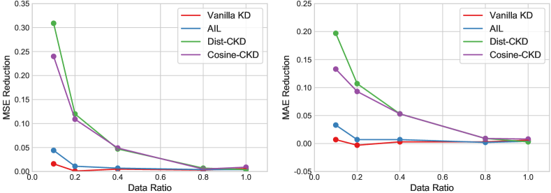
Figure 3: The MSE (left) and MAE (right) reduction curve over the non-distillation methods with varying dataset sizes of different distillation objective on the hourly dataset. Our distributional correlation-aware distillation boosts the performance more significantly under low-resource settings. Best viewed in color.

Our findings are: (1) The performance gain of distillation vanishes as the data size becomes larger. It is reasonable as the small training dataset cannot provide comprehensive supervision, while the extra information in the teacher predictions can alleviate this problem. As the size of the training dataset increases, the training samples cover more diverse data patterns, thus the student can directly learn from the supervision provided by the original data samples instead of relying on the teacher predictions. This is consistent with previous studies which observe that KD brings more performance boost on small datasets [29, 17]. (2) Compared with distillation methods solely based on the predicted scalar values, the proposed Dist-CKD and Cosine-CKD boost the performance more significantly under low-resource settings. We attribute the success to the more informative supervision brought by the distributional correlational-aware distillation objectives, which helps the student make more accurate predictions even with few training samples. (3) Dist-CKD reduces prediction error more under low-resource settings while Cosine-CKD outperforms the Dist-CKD with the full training dataset. We attribute the reason to that the cosine similarity is a higher-order property than the distance-wise similarity, it may require more data samples to fully exploit its effectiveness.

4.3 Correlational Objectives Improve Magnitude Ordering

We are interested in that whether the proposed correlational objective help the model learn the relation between the output trading volumes, which can facilitate better trading decisions. To investigate this, we calculate the pair-wise relations, i.e., the relative trading magnitude between samples, and probe the relation consistency between the model predictions and the oracle trading volume. Specifically, given $N$ data samples and the corresponding oracle volume $y_{1},\ldots,y_{N}$, we define the error ranking score as:

Error Ranking Number $$=\sum_{i=1}^{N}\sum_{j=1,j\neq i}^{N}\text{ErrorSign}\left(\left(y_{i}-y_{j}\right)\times\left(\hat{y}_{i}-\hat{y}_{j}\right)\right),$$ (16)

$$\operatorname{ErrorSign}\left(x\right) =\begin{cases}1&\text{ if }x\leq 0,\\ 0&\text{ otherwise. }\end{cases}$$

This metric indicates how many pairs of data samples whose relative trading volume magnitude are mispredicted by the model. We randomly sampled $12,000$ data samples from the test set and calculate the metric. The results are shown in Table 4.

Table 4: Examining the Error Ranking Number of different methods on datasets with different time window settings. The best results are shown in bold.

Dataset	Hourly	Daily
Model	Error Ranking Number ($\downarrow$)	Error Ranking Number ($\downarrow$)
Min-MSE	20,545,150	14,781,916
Vanilla KD [9]	20,011,092	14,369,730
AIL [27]	20,026,808	14,580,932
DeepAR [25]	20,042,538	14,490,082
DKD	20,036,694	14,363,378
w/ Dist-CKD	19,841,196	14,294,670
w/ Cosine-CKD	19,930,742	14,393,534

Our observations are: (1) Distillation methods are effective for improving the prediction consistency with the oracle model. Compared with training the student model with the original mean-square error loss objective, Vanilla KD and AIL both greatly reduce the error ranking number. This shows that transferring the knowledge from the teacher model to the student not only improves the student prediction accuracy, but also makes the student become more aware of the relative magnitude between predictions. (2) Our methods achieve the best performance on both datasets. For example, on the hourly dataset, compared with the Min-MSE method, Dist-CKD reduces the Error Ranking Number by $3.4\%$, which verifies that our proposed correlational distillation objectives can help the model learn the relative trading volume magnitude better. Besides, Dist-CKD performs consistently better than Cosine-CKD regarding the trading volume magnitude relationship, which we attribute to the fact that the distance correlation defined in Eq. 11 is a more explicit modeling of the magnitude relation than the angle-wise objective.

5 Related Work

5.1 Knowledge Distillation

Neural network compression can produce light-weight models for efficient deployments, and it has been an active research area towards green and sustainable deep learning [31, 16, 14]. Knowledge distillation [9, 24] transfers the knowledge of a larger teacher to a smaller student model, achieving a better trade-off between model performance and inference efficiency. Recent studies show that KD is effective in computer vision [23, 21] and natural language processing [29, 13], successfully training a compact student model to perform on par with the large teacher model. While previous studies focus on classification problems, in this paper, we explore knowledge distillation for obtaining a compact student model to perform time series forecasting. We build a distributional level knowledge distillation framework for trading volume prediction and propose two correlation-aware distillation objectives. Our work is partially inspired by [23], which aligns the pair-wise correlations of data representations in the teacher and the student model. However, our framework focuses on the relationship of output distributions. Their method thus is orthogonal to our method and can be incorporated into our framework for further performance boost. Besides, to the best of our knowledge, we are the first to conduct knowledge distillation for the trading volume prediction problem and prove it is effective for obtaining light-weight and well-performing models.

5.2 Volume Prediction

Stock trading volume prediction has a significant role in algorithmic trading systems [2, 3, 4], which aims to predict the stock trading volume based on preceding transaction data. Recently, progresses have been made towards more accurate volume prediction via various machine learning techniques. Specifically, [19] propose to adopt support vector machine (SVM) for the regression problem to predict the changes of volume percentage. [18] exploit long short-term memory (LSTM) models [10] for its capability of modeling long-range dependency. Besides, temporal mixture ensemble models [1], Bayesian auto-regressive models [12] and graph neural networks [33] are also explored in volume prediction. [32] train a Transformer model [30] with adversarial objectives to improve the model performance and robustness at the same time. In this paper, we focus on distilling a more efficient trading volume prediction model and adopt the powerful Transformer as the backbone model for distillation. Our framework is generalizable and can be easily extended to other backbone models.

6 Conclusion

In this paper, we present a distributional knowledge distillation framework for training light-weight trading volume prediction models. The learned knowledge of the teacher model is transferred to the student model at the distributional level, by minimizing the KL-divergence between the predicted Gaussian distributions and the distance-wise and angle-wise correlation distillation objectives. Experiments on the TPX500 dataset with two different time window settings show that our framework can effectively compress the model while maintaining accurate predictions. Further analysis shows that the correlational objectives significantly boost the student performance under low-resource settings and make the predictions more consistent with the oracle labels. In the future, we are hoping to explore this framework for more general regression tasks.

Appendix 0.A Cosine Similarity of Gaussian Distributions

Proof

The inner-dot and the cosine similarity of $\mathcal{N}_{i}\left(\mu_{i},\sigma_{i}\right)$ and $\mathcal{N}_{j}\left(\mu_{j},\sigma_{j}\right)$ are:

$$(\mathcal{N}_{i},\mathcal{N}_{j}) =\int_{-\infty}^{+\infty}\mathcal{N}_{i}(t\mid\mu_{i},\sigma_{i})\mathcal{N}_{j}(t\mid\mu_{j},\sigma_{j})dt$$

$$=\int_{-\infty}^{+\infty}\frac{1}{2\pi\sigma_{i}^{2}\sigma_{j}^{2}}\exp\left(-\frac{(t-\mu_{i})^{2}}{2\sigma_{i}^{2}}-\frac{(t-\mu_{j})^{2}}{2\sigma_{j}^{2}}\right)dt$$

$$=\int_{-\infty}^{+\infty}\frac{1}{2\pi\sigma_{i}\sigma_{j}}\exp\left(-\frac{(t-\mu^{\prime})^{2}}{2\frac{\sigma_{i}^{2}\sigma_{j}^{2}}{\sigma_{i}^{2}+\sigma_{j}^{2}}}-\frac{(\mu_{i}-\mu_{j})^{2}}{2(\sigma_{i}^{2}+\sigma_{j}^{2})}\right)dt$$

$$=\frac{1}{\sqrt{2\pi(\sigma_{i}^{2}+\sigma_{j}^{2})}}\exp\left(-\frac{(\mu_{i}-\mu_{j})^{2}}{2(\sigma_{i}^{2}+\sigma_{j}^{2})}\right)$$

where $\mu^{\prime}=\frac{\mu_{i}\sigma_{j}^{2}+\mu_{j}\sigma_{i}^{2}}{\sigma_{i}^{2}+\sigma_{j}^{2}}$, $(\mathcal{N}_{i},\mathcal{N}_{i})=\frac{1}{\sqrt{4\pi\sigma_{i}^{2}}},(\mathcal{N}_{j},\mathcal{N}_{j})=\frac{1}{\sqrt{4\pi\sigma_{j}^{2}}}$,

$$\varphi_{\text{Cosine}}\left(\mathcal{N}_{i},\mathcal{N}_{j}\right) =\frac{(\mathcal{N}_{i},\mathcal{N}_{j})}{\sqrt{(\mathcal{N}_{i},\mathcal{N}_{i})(\mathcal{N}_{j},\mathcal{N}_{j})}}$$

$$=\frac{\sqrt{(4\pi\sigma_{i}^{2})^{\frac{1}{2}}(4\pi\sigma_{j}^{2})^{\frac{1}{2}}}}{\sqrt{2\pi(\sigma_{i}^{2}+\sigma_{j}^{2})}}\exp\left(-\frac{(\mu_{i}-\mu_{j})^{2}}{2(\sigma_{i}^{2}+\sigma_{j}^{2})}\right)$$

$$=\sqrt{\frac{2\sigma_{i}\sigma_{j}}{{\sigma_{i}^{2}+\sigma_{j}^{2}}}}\exp\left(-\frac{\left(\mu_{i}-\mu_{j}\right)^{2}}{2\left(\sigma_{i}^{2}+\sigma_{j}^{2}\right)}\right)$$

References

- [1] Antulov-Fantulin, N., Guo, T., Lillo, F.: Temporal mixture ensemble models for intraday volume forecasting in cryptocurrency exchange markets. arXiv: Trading and Market Microstructure (2020)
- [2] Białkowski, J., Darolles, S., Le Fol, G.: Improving vwap strategies: A dynamic volume approach. Journal of Banking & Finance 32(9), 1709–1722 (2008)
- [3] Brownlees, C.T., Cipollini, F., Gallo, G.M.: Intra-daily volume modeling and prediction for algorithmic trading. Journal of Financial Econometrics 9(3), 489–518 (2011)
- [4] Cartea, Á., Jaimungal, S.: A closed-form execution strategy to target volume weighted average price. SIAM Journal on Financial Mathematics 7(1), 760–785 (2016)
- [5] Devlin, J., Chang, M.W., Lee, K., Toutanova, K.: BERT: Pre-training of deep bidirectional transformers for language understanding. In: NAACL-HLT. pp. 4171–4186 (2019)
- [6] Dosovitskiy, A., Beyer, L., Kolesnikov, A., Weissenborn, D., Zhai, X., Unterthiner, T., Dehghani, M., Minderer, M., Heigold, G., Gelly, S., et al.: An image is worth 16x16 words: Transformers for image recognition at scale. In: ICLR (2020)
- [7] Furlanello, T., Lipton, Z.C., Tschannen, M., Itti, L., Anandkumar, A.: Born-again neural networks. In: ICML. Proceedings of Machine Learning Research, vol. 80, pp. 1602–1611 (2018)
- [8] Han, S., Mao, H., Dally, W.J.: Deep compression: Compressing deep neural networks with pruning, trained quantization and huffman coding. arXiv preprint arXiv:1510.00149 (2015)
- [9] Hinton, G., Vinyals, O., Dean, J.: Distilling the knowledge in a neural network. arXiv preprint arXiv:1503.02531 (2015)
- [10] Hochreiter, S., Schmidhuber, J.: Long short-term memory. Neural computation 9(8), 1735–1780 (1997)
- [11] Hubara, I., Courbariaux, M., Soudry, D., El-Yaniv, R., Bengio, Y.: Binarized neural networks. In: NeurIPS. pp. 4107–4115 (2016)
- [12] Huptas, R.: Point forecasting of intraday volume using bayesian autoregressive conditional volume models. Journal of Forecasting (2018)
- [13] Jiao, X., Yin, Y., Shang, L., Jiang, X., Chen, X., Li, L., Wang, F., Liu, Q.: Tinybert: Distilling bert for natural language understanding. In: Findings of the Association for Computational Linguistics: EMNLP 2020. pp. 4163–4174 (2020)
- [14] Li, L., Lin, Y., Chen, D., Ren, S., Li, P., Zhou, J., Sun, X.: CascadeBERT: Accelerating inference of pre-trained language models via calibrated complete models cascade. In: Findings of the Association for Computational Linguistics: EMNLP. pp. 475–486 (2021)
- [15] Li, L., Lin, Y., Ren, S., Li, P., Zhou, J., Sun, X.: Dynamic knowledge distillation for pre-trained language models. In: EMNLP. pp. 379–389 (2021)
- [16] Li, L., Lin, Y., Ren, X., Zhao, G., Li, P., Zhou, J., Sun, X.: Model uncertainty-aware knowledge amalgamation for pre-trained language models. arXiv preprint arXiv:2112.07327 (2021)
- [17] Liang, K.J., Hao, W., Shen, D., Zhou, Y., Chen, W., Chen, C., Carin, L.: MixKD: Towards efficient distillation of large-scale language models. In: ICLR (2021)
- [18] Libman, D.S., Haber, S., Schaps, M.: Volume prediction with neural networks. Frontiers in Artificial Intelligence 2 (2019)
- [19] Liu, X., Lai, K.K.: Intraday volume percentages forecasting using a dynamic svm-based approach. Journal of Systems Science and Complexity 30(2), 421–433 (2017)
- [20] Loshchilov, I., Hutter, F.: Decoupled weight decay regularization. In: ICLR (2019)
- [21] Mirzadeh, S., Farajtabar, M., Li, A., Levine, N., Matsukawa, A., Ghasemzadeh, H.: Improved knowledge distillation via teacher assistant. In: AAAI. pp. 5191–5198 (2020)
- [22] Pardo, L.: Statistical inference based on divergence measures. Chapman and Hall/CRC (2018)
- [23] Park, W., Kim, D., Lu, Y., Cho, M.: Relational knowledge distillation. In: CVPR. pp. 3967–3976 (2019)
- [24] Romero, A., Ballas, N., Kahou, S.E., Chassang, A., Gatta, C., Bengio, Y.: Fitnets: Hints for thin deep nets. In: ICLR (2015)
- [25] Salinas, D., Flunkert, V., Gasthaus, J., Januschowski, T.: Deepar: Probabilistic forecasting with autoregressive recurrent networks. International Journal of Forecasting 36(3), 1181–1191 (2020)
- [26] Sanh, V., Debut, L., Chaumond, J., Wolf, T.: DistilBERT, a distilled version of BERT: smaller, faster, cheaper and lighter. In: NeurIPS Workshop on Energy Efficient Machine Learning and Cognitive Computing (2019)
- [27] Saputra, M.R.U., de Gusmão, P.P.B., Almalioglu, Y., Markham, A., Trigoni, N.: Distilling knowledge from a deep pose regressor network. In: ICCV. pp. 263–272 (2019)
- [28] Shen, S., Dong, Z., Ye, J., Ma, L., Yao, Z., Gholami, A., Mahoney, M.W., Keutzer, K.: Q-BERT: Hessian based ultra low precision quantization of BERT. In: AAAI. pp. 8815–8821 (2020)
- [29] Sun, S., Cheng, Y., Gan, Z., Liu, J.: Patient knowledge distillation for BERT model compression. In: EMNLP-IJCNLP. pp. 4323–4332 (2019)
- [30] Vaswani, A., Shazeer, N., Parmar, N., Uszkoreit, J., Jones, L., Gomez, A.N., Kaiser, L., Polosukhin, I.: Attention is all you need. In: NeurIPS. pp. 5998–6008 (2017)
- [31] Xu, J., Zhou, W., Fu, Z., Zhou, H., Li, L.: A survey on green deep learning. arXiv preprint arXiv:2111.05193 (2021)
- [32] Zhang, Z., Li, W., Bao, R., Harimoto, K., Wu, Y., Sun, X.: ASAT: Adaptively scaled adversarial training in time series. arXiv preprint arXiv:2108.08976 (2021)
- [33] Zhao, L., Li, W., Bao, R., Harimoto, K., Wu, Y., Sun, X.: Long-term, short-term and sudden event: Trading volume movement prediction with graph-based multi-view modeling. In: Zhou, Z. (ed.) IJCAI. pp. 3764–3770 (2021)