A Semi-analytical Method of Calculating Nuclear Collision Trajectory in the QCD Phase Diagram

Abstract

The finite nuclear thickness affects the energy density $\epsilon(t)$ and conserved-charge densities such as the net-baryon density $n_{B}(t)$ produced in heavy ion collisions. While the effect is small at high collision energies where the Bjorken energy density formula for the initial state is valid, the effect is large at low collision energies, where the nuclear crossing time is not small compared to the parton formation time. The temperature $T(t)$ and chemical potentials $\mu(t)$ of the dense matter can be extracted from the densities for a given equation of state (EOS). Therefore, including the nuclear thickness is essential for the determination of the $T$-$\mu_{B}$ trajectory in the QCD phase diagram for relativistic nuclear collisions at low to moderate energies such as the RHIC-BES energies. In this proceeding, we will first discuss our semi-analytical method that includes the nuclear thickness effect and its results on the densities $\epsilon(t),n_{B}(t),n_{Q}(t)$, and $n_{S}(t)$. Then, we will show the extracted $T(t),\mu_{B}(t),\mu_{Q}(t)$, and $\mu_{S}(t)$ for a quark-gluon plasma using the ideal gas EOS with quantum or Boltzmann statistics. Finally, we will show the results on the $T$-$\mu_{B}$ trajectories in relation to the possible location of the QCD critical end point. This semi-analytical model provides a convenient tool for exploring the trajectories of nuclear collisions in the QCD phase diagram.

I Introduction

The study of the QCD phase diagram, including the possible critical end point (CEP) that separates the crossover transition from a first-order transition, is a focus of relativistic heavy ion physicsStephanov (2004); Aggarwal et al. (2010); Adam et al. (2021). For this purpose, it is important to calculate or estimate the collision trajectory in the QCD phase diagram in the $T-\mu_{B}$ plane or the general $T-\mu_{B}-\mu_{Q}-\mu_{S}$ four-dimensional space. So far, this is mostly done by analyzing the time evolution of given volume cells in dynamical models Arsene et al. (2007); Wang et al. (2022) such as transport models and hydrodynamical models, which usually takes a lot of effort. A trajectory can also be estimated by using a given equation of state with assumptions such as imposing a constant $s/n_{B}$ (entropy to net-baryon-density ratio) along the trajectory Noronha-Hostler et al. (2019). In this approach, extra information is needed to determine the endpoint of the trajectory at the maximum energy density.

Here we present a semi-analytical method Mendenhall and Lin (2021a) to calculate the trajectory of central nuclear collisions in the QCD phase diagram. It is straightforward to reproduce and already available online int (2022). It also allows us to have analytical understanding of the effects of the finite nuclear thickness and parton formation time on the collision trajectories of different collision systems at different energies. The method first calculates the time evolution of four densities: the energy density $\epsilon$, net-baryon density $n_{B}$, net-electric-charge density $n_{Q}$, and net-strangeness density $n_{S}$. We then use a given EOS to convert them to four thermodynamic quantities: $T,\mu_{B},\mu_{Q}$, and $\mu_{S}$.

A famous semi-analytical result on the energy density is the Bjorken energy density formula for mid-spacetime-rapidity Bjorken (1983):

$$\epsilon^{Bj}(t)=\frac{1}{tA_{T}}\frac{dE_{T}}{dy}.$$ (1)

In the above, $A_{T}=\pi R_{A}^{2}$ is the transverse overlap area of the two nuclei in central collisions, $R_{A}=1.12A^{1/3}$ fm is the nuclear radius in the hard-sphere model, and $dE_{T}/dy$ is the transverse energy rapidity density at mid-rapidity. The formula is mostly used to estimate the energy density of the initial state, where time $t$ is chosen as the formation time of the quark-gluon plasma or the produced partons ($\tau_{F}$). Note that the formula also applies to any time $t$ after $\tau_{F}$ when the partons are assumed to be free-streaming; it thus describes the time evolution of the energy density produced from the initial state when the subsequent parton interactions and transverse expansion are neglected.

However, the Bjorken energy density formula breaks down at low energies where the nuclear crossing time is not small compared to $\tau_{\rm{}_{F}}$. In the hard sphere model for the nucleus, the crossing time is given by $d_{t}=2R_{A}/(\beta\gamma)$, where $\beta$ is the speed of the projectile nucleus in the center-of-mass frame and $\gamma=1/\sqrt{1-\beta^{2}}$ is the corresponding Lorentz factor. Obviously, the crossing time becomes bigger at lower energies, where its effect must be considered. Therefore, we have extended the Bjorken formula, first by including the finite time (but neglecting the finite width along the beam direction $z$) of the initial energy production Lin (2018), and later by including both the finite time and finite width in $z$ Mendenhall and Lin (2021b). Figure 1 shows the schematic picture in the $z-t$ plane for calculating the energy density at mid-spacetime-rapidity (inside $-d<z<d$ at finite time $t$ with $d\to 0$) for central A+A collisions. The Bjorken formula Bjorken (1983) assumes that partons are initially produced at $z_{0}=0$ and time $0$, and the first extension Lin (2018) assumes that partons are initially produced at $z_{0}=0$ but at any time within $[0,d_{t}]$. In the second extension Mendenhall and Lin (2021b), partons can be initially produced anywhere inside the rhombus, which is within $z_{0}\in[-\beta d_{t}/2,\beta d_{t}/2]$ and time $\in[0,d_{t}]$. Note that parton interactions after their initial productions are neglected in all three methods.

In the second extension study that considers the full finite thickness effect Mendenhall and Lin (2021b), the initial energy density at time $t$ averaged over the full transverse overlap area can be written as

$$\epsilon(t)=\frac{1}{A_{T}}\int_{S}\frac{dxdz_{0}}{t-x}\frac{d^{3}m_{T}}{dxdz_{0}dy}\cosh^{3}y.$$ (2)

Here, $S$ represents the production area over the initial production time $x$ and longitudinal position $z_{0}$ at observation time $t$, as indicated by the shaded area in Fig.1. For the transverse energy density $d^{3}m_{T}/(dxdz_{0}dy)$, we make the simplest assumption that it is uniform over the $z_{0}-x$ plane, i.e., $d^{3}m_{T}/(dxdz_{0}dy)\propto dm_{T}/dy$. After parameterizing the $dm_{T}/dy$ function with the measured transverse energy rapidity density and net-proton $dN/dy$ Mendenhall and Lin (2021b), we can then calculate the time evolution of the energy density. We apply the same method to calculate the time evolution of the net-charge densities Mendenhall and Lin (2021a). For example, the net-baryon density from our semi-analytical model is given by

$$n_{B}(t)=\frac{1}{A_{T}}\int_{S}\frac{dxdz_{0}}{t-x}\frac{d^{3}N_{B}}{dxdz_{0}dy}\cosh^{2}{y},$$ (3)

where $N_{B}$ represents the net-baryon number in an event. On the other hand, the net-baryon density in the Bjorken model is given by

$$n_{B}^{Bj}(t)=\frac{1}{tA_{T}}\frac{dN_{B}}{dy}.$$ (4)

Details of the calculations including the parameterizations of $dm_{T}/dy$ and the net-proton $dN/dy$ can be found in the full studies Mendenhall and Lin (2021b, a). Note that our method enforces the relevant conservation laws, i.e., the produced matter in a central heavy ion collision is assumed to have a total energy $A\sqrt{s_{\rm{}_{NN}}}$, total net-baryon number $2A$, total net-charge $2Z$, and total net-strangeness 0.

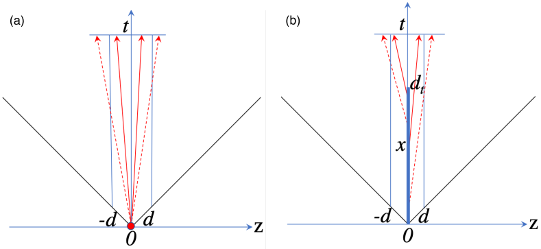
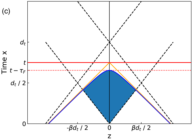
Figure 1: Schematic diagram for the crossing of two identical nuclei for (a) the Bjorken $\epsilon$ formula, (b) the method that considers the finite crossing time but not the finite longitudinal width Lin (2018), and (c) the current method that considers the full crossing diamond area Mendenhall and Lin (2021b). In (c), partons can be produced anywhere inside the rhombus, the solid diagonal lines represent the light cone boundaries for partons that can reach $z\approx 0$ at time $t$, while the hyperbola represents the boundary of these partons after considering the formation time $t_{F}=\tau_{F}\,{\rm\cosh}\,y$.

II Results

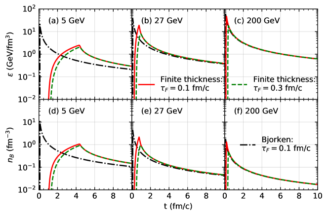
Figure 2: (a-c) Energy density $\epsilon(t)$ and (d-f) net-baryon density $n_{B}(t)$ at mid-rapidity for central Au+Au collisions at $\sqrt{s_{\rm{}_{NN}}}=$5, 27 and 200 GeV from our model for $\tau_{F}=0.1$ and $0.3$ fm/$c$ in comparison with the Bjorken formula for $\tau_{F}=0.1$ fm/$c$.

The top panels of Fig. 2 show the results of $\epsilon(t)$, the average energy density at mid-rapidity as calculated with Eq.(2), for central Au+Au collisions at three different energies. The results from our semi-analytical model at $\tau_{F}=0.1$ (solid) and $0.3$ (dashed) fm/$c$ are shown in comparison with the results from the Bjorken energy density formula at $\tau_{F}=0.1$ fm/$c$ (dot-dashed). The lower panels show the corresponding results of the net-baryon density $n_{B}(t)$. Compared to the results from the Bjorken formula, our results show significantly lower peak values, $\epsilon^{max}$ and $n_{B}^{max}$, at lower collision energies, as expected from earlier studies of the effect of the finite nuclear thickness Lin (2018); Mendenhall and Lin (2021b). At high collision energies, our results approach the Bjorken formula. We also see that the peak energy density $\epsilon^{max}$ increases as $\sqrt{s_{\rm{}_{NN}}}$ increases, while the peak net-baryon density $n_{B}^{max}$ first increases and then decreases with $\sqrt{s_{\rm{}_{NN}}}$. Note that for the net-charge and net-strangeness densities, our semi-analytical method gives the following:

$$n_{Q}(t)=\frac{Z}{A}n_{B}(t),~{}n_{S}(t)=0.$$ (5)

Note that the above relations are often used to constrain the equation of state such as those from lattice QCD calculations Noronha-Hostler et al. (2019).

After calculating the densities, we can then use a given equation of state of the nuclear matter to convert them into the thermodynamical quantities: temperature $T$ and chemical potentials $\mu$. In this proceeding, we use the ideal gas quark-gluon plasma EOS with quantum or Boltzmann statistics for the conversions Mendenhall and Lin (2021a). The solid curves in Fig. 3 show the $T$ and $\mu$ results for central Au+Au collisions at $\tau_{\rm{}_{F}}=0.1$ fm/$c$, which are extracted from the full solution of the quantum ideal gas EOS, i.e., by solving the four equations relating $\epsilon,n_{B},n_{Q}$, and $n_{S}$ to $T,\mu_{B},\mu_{Q}$, and $\mu_{S}$. We can see that the peak temperature $T^{max}$ increases with $\sqrt{s_{\rm{}_{NN}}}$, while the peak net-baryon chemical potential $\mu_{B}^{max}$ decreases with $\sqrt{s_{\rm{}_{NN}}}$. In addition, both $T^{max}$ and $\mu_{B}^{max}$ are reached earlier at higher energies due to the shorter crossing time.

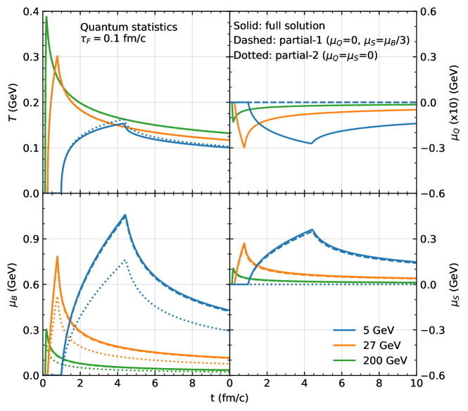
Figure 3: The extracted $T(t)$, $\mu_{B}(t)$, $\mu_{Q}(t)$, and $\mu_{S}(t)$ for $\tau_{\rm{}_{F}}=0.1$ fm/$c$ from the full solution or partial solutions of the quantum ideal gas EOS for central Au+Au collisions at 5, 27, and 200 GeV. Note that the $\mu_{Q}(t)$ curves have been multiplied by a factor of 10.

If we are only interested in the collision trajectory in the $T-\mu_{B}$ plane (instead of the four-dimensional $T-\mu$ space) of the QCD phase diagram, it would be convenient to have the (partial) relations between $\epsilon,n_{B}$ and $T,\mu_{B}$ without the net-charge or net-strangeness variables. The easiest way to achieve this, which has often been used  Noronha-Hostler et al. (2019); Grefa et al. (2021), is to assume $\mu_{Q}=\mu_{S}=0$. We name the resultant relations as the partial-2 solution of the EOS. However, this assumption violates the strangeness neutrality condition $n_{S}=0$ that is expected for heavy ion collisions. Indeed, we see from Fig. 3 that the partial-2 solution (dotted curves) gives a much smaller $\mu_{B}$ than the full solution and thus cannot give accurate trajectories.

An alternative way is to assume the following:

$$\mu_{Q}=0,~{}\mu_{S}=\frac{\mu_{B}}{3},$$ (6)

and we name the resultant relations as the partial-1 solution of the EOS. The assumption $\mu_{Q}=0$ is made because the $\mu_{Q}$ values extracted from the full solution are very small, as shown in the upper-right panel of Fig.3 where the $\mu_{Q}$ values have been multiplied by a factor of 10. The smallness of $\mu_{Q}$ is a consequence of the fact that most nuclei have $Z\sim A/2$, because the strangeness neutrality $n_{S}=0$ plus the condition $n_{Q}=n_{B}/2$ would lead to $\mu_{Q}=0$ for either the quantum or Boltzmann ideal gas EOS Mendenhall and Lin (2021a). The other assumption $\mu_{S}=\mu_{B}/3$ is made to satisfy the strangeness neutrality, which requires $\mu_{B}-\mu_{Q}-3\mu_{S}=0$ for the QGP ideal gas equations of state Mendenhall and Lin (2021a). Note that the recent numerical results of the collision trajectories from the AMPT model Wang et al. (2022) also show $\mu_{Q}\approx 0$ and $\mu_{S}\approx\mu_{B}/3$. In the left panels of Fig.3, we see that the $T(t)$ and $\mu_{B}(t)$ results from the partial-1 solution and those from the full solution agree very well. This demonstrates that the partial-1 solution and its following relations from the quantum ideal gas EOS are quite accurate, at least for the QGP ideal gas equations of state:

$$\begin{split}\epsilon_{1}&=\frac{19\pi^{2}}{12}T^{4}+\frac{\mu_{B}^{2}}{3}T^{2}+\frac{\mu_{B}^{4}}{54\pi^{2}},\\ n_{B,1}&=\frac{2\mu_{B}}{9}T^{2}+\frac{2\mu_{B}^{3}}{81\pi^{2}}.\end{split}$$ (7)

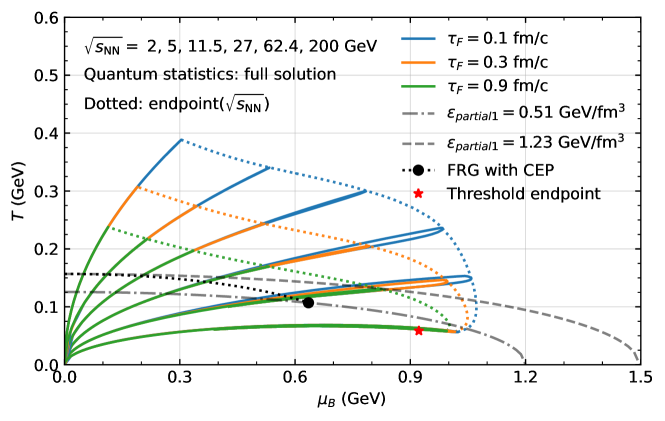
Figure 4: Trajectories for the quantum ideal gas EOS at $\tau_{\rm{}_{F}}=$ 0.1, 0.3, and 0.9 fm/$c$ for central Au+Au collisions at different energies, together with the trajectory endpoint curves for $\sqrt{s_{\rm{}_{NN}}}$ from 2 to 200 GeV. The endpoint at the threshold energy is shown as star. The FRG crossover curve with the critical end point is also shown, where the two constant energy density curves from the partial-1 solution intersect the endpoints of the FRG curve.

Figure 4 shows the $T-\mu_{B}$ trajectories in the QCD phase diagram for the quantum ideal gas EOS at three different $\tau_{\rm{}_{F}}$ values for central Au+Au collisions at different energies. The QCD crossover curve and the critical end point at $(\mu_{B},T)=(0.635{\rm~{}GeV},0.107{\rm~{}GeV})$, calculated from the functional renormalization group (FRG) with $N_{F}=2+1$ Fu et al. (2020), are also shown. We have also used the quantum partial-1 solution Eq.(7) to calculate the lines of constant $\epsilon$, which go through the two endpoints of the FRG crossover curve at $\epsilon=1.23$ (dashed) and 0.51 (dot-dashed) GeV/fm³. At the threshold energy $\sqrt{s_{\rm{}_{NN}}}=2m_{N}$ with $m_{N}$ being the nucleon mass, our model gives $\epsilon^{max}=2\rho_{0}m_{N}$ and $n_{B}^{max}=2\rho_{0}$ Mendenhall and Lin (2021a) ($\rho_{0}\approx 0.17$ fm^-3), which would be expected if the two nuclei would just fully overlap. If we treat this matter as an ideal gas QGP with quantum statistics, it will be located at $(\mu_{B},T)\sim(0.9{\rm~{}GeV},0.06{\rm~{}GeV})$, as shown by the star symbol in Fig. 4. When a trajectory reaches the endpoint, where both $\epsilon^{max}$ and $n_{B}^{max}$ are reached, it turns clockwise and returns toward the origin. We see that the returning part of the trajectory almost overlaps with the outgoing part at high collision energies. In addition, the trajectories in Fig. 4 pass through the crossover curve for central Au+Au collisions at $\sqrt{s_{\rm{}_{NN}}}\gtrsim 4$ GeV.

The results from our semi-analytical model  Lin (2018); Mendenhall and Lin (2021b, a) depend on the value of $\tau_{\rm{}_{F}}$, and Fig. 4 also shows how the $T-\mu_{B}$ trajectories from the quantum ideal gas EOS depend on $\tau_{\rm{}_{F}}$. At a smaller $\tau_{\rm{}_{F}}$, the peak densities are higher; therefore, the trajectory becomes longer with the endpoint moving further to higher $\mu_{B}$ (and also higher $T$ except at very low energies). The endpoints of the trajectories as functions of the collision energy are shown by the three colored dotted curves in Fig. 4 for three different formation times. We observe a clear separation of the endpoint curves of different $\tau_{\rm{}_{F}}$ values, except for very low collision energies, where the endpoint curves become less sensitive to $\tau_{\rm{}_{F}}$. This is expected because the densities such as the energy density depend on $\tau_{\rm{}_{F}}$ weakly at low collision energies but strongly ($\propto 1/\tau_{\rm{}_{F}}$) at high energies Mendenhall and Lin (2021b). We also see in Fig. 4 that even for the relatively large value of $\tau_{\rm{}_{F}}=0.9$ fm/$c$, the CEP from the FRG calculation is within the coverage of the trajectory endpoint curve.

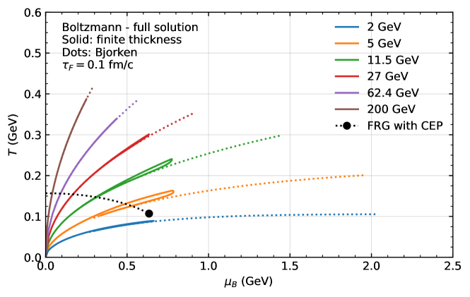
Figure 5: Trajectories for the Boltzmann ideal gas EOS for central Au+Au collisions at different energies from our method and the Bjorken formula for $\tau_{\rm{}_{F}}=0.1$ fm/$c$. The FRG crossover curve with the CEP is also shown.

To see the effect of the finite nuclear thickness, in Fig. 5 we compare our trajectories with the Bjorken trajectories, i.e., trajectories extracted from the $\epsilon(t)$ and $n_{B}(t)$ values calculated with the Bjorken formula, for the Boltzmann ideal gas EOS. At high collision energies, our trajectories are rather close to the Bjorken trajectories as expected. At lower collision energies, however, the $\mu_{B}^{max}$ value from the Bjorken trajectory is much larger because of its much higher peak density $n_{B}^{max}$. In addition, we see in Fig. 5 that the late-time part of the Bjorken trajectory overlaps with the returning part of our trajectory. This is expected because at late times our semi-analytical model approaches the Bjorken formula Lin (2018); Mendenhall and Lin (2021b), which can be seen in Fig. 2.

By comparing the trajectories from the quantum ideal gas EOS in Fig. 4 and those from the Boltzmann ideal gas EOS in Fig. 5, we can see that the trajectory depends on the equation of state. While the $T^{max}$ values are often similar at the same collision energy (except for very low energies), the $\mu_{B}^{max}$ value is significantly larger in the quantum ideal gas EOS. This feature is also seen in the trajectories calculated from the AMPT model Wang et al. (2022) and can be understood in terms of the Pauli exclusion principle in the quantum EOS.

III Summary and outlook

We have developed a semi-analytical model to calculate the time-dependent energy density $\epsilon(t)$, net-baryon density $n_{B}(t)$, net-electric-charge density $n_{Q}(t)$, and net-strangeness density $n_{S}(t)$ at mid-pseudorapidity averaged over the transverse overlap area in central Au+Au collisions. We then extract the time evolution of the thermodynamical quantities $T,\mu_{B},\mu_{Q}$, and $\mu_{S}$ assuming the formation of a QGP with either quantum or Boltzmann ideal gas equation of state. This enables us to plot the collision trajectories in the $T-\mu_{B}$ plane of the QCD phase diagram.

The trajectories from our model are very different from those calculated with the Bjorken formula at energies below tens of GeVs, demonstrating the importance of including the finite nuclear thickness at those energies. We also find that the accessible area in the phase diagram depends strongly on the parton formation time $\tau_{F}$ when the collision energy is higher than a few GeVs. However, even when using a relatively large $\tau_{F}$ value of 0.9 fm$/c$, the critical end point from the FRG calculation is within the area covered by the trajectories. We also find that the $T-\mu_{B}$ results from the simpler partial solution that assumes $\mu_{Q}=0$ and $\mu_{S}=\mu_{B}/3$ are very close to the full solution. On the other hand, the results from another partial solution that assumes $\mu_{Q}=\mu_{S}=0$, which violates the strangeness neutrality, significantly underestimate the extracted $\mu_{B}$ values.

We find that the collision trajectory depends on the equation of state. For our results from the ideal gas equations of state for the quark-gluon plasma, the calculated trajectory should break down soon after it goes below the crossover curve (or the first-order phase transition curve) in the QCD phase diagram. We plan to extend this study by using more realistic equations of state, such as those based on the lattice QCD calculations Noronha-Hostler et al. (2019). In addition, we have so far neglected the transverse expansion of the created matter, which would decrease the peak densities and thus affect the collision trajectory in the phase diagram. We also plan to include this effect in the update of the full study Mendenhall and Lin (2021a).

We have written a web interface int (2022), which will plot the calculated energy density as a function of time as well as the event trajectory in the T-$\mu_{B}$ plane according to the user’s input for the colliding system, energy and formation time $\tau_{\rm{}_{F}}$. A data file for the time evolution of the energy density, temperature, and the three chemical potentials can also be downloaded. So far only the ideal gas equations of state are implemented at the web interface, and we plan to add a more realistic equation of state. We hope that this semi-analytical model will provide the community a useful tool for exploring the trajectories of nuclear collisions in the QCD phase diagram in the $T-\mu_{B}$ plane or the general $T-\mu_{B}-\mu_{Q}-\mu_{S}$ space.

References

References

- Stephanov (2004) M. A. Stephanov, Prog. Theor. Phys. Suppl. 153, 139 (2004).
- Aggarwal et al. (2010) M. M. Aggarwal et al. (STAR), Phys. Rev. Lett. 105, 022302 (2010).
- Adam et al. (2021) J. Adam et al. (STAR), Phys. Rev. Lett. 126, 092301 (2021).
- Arsene et al. (2007) I. C. Arsene et al., Phys. Rev. C 75, 034902 (2007).
- Wang et al. (2022) H.-S. Wang, G.-L. Ma, Z.-W. Lin, and W.-j. Fu, Phys. Rev. C 105, 034912 (2022).
- Noronha-Hostler et al. (2019) J. Noronha-Hostler, P. Parotto, C. Ratti, and J. M. Stafford, Phys. Rev. C 100, 064910 (2019).
- Mendenhall and Lin (2021a) T. Mendenhall and Z.-W. Lin, arXiv:2111.13932 [nucl-th] (2021a).
- int (2022) A web interface that performs our semi-analytical calculation is available at http://myweb.ecu.edu/linz/densities/ (2022).
- Bjorken (1983) J. D. Bjorken, Phys. Rev. D 27, 140 (1983).
- Lin (2018) Z.-W. Lin, Phys. Rev. C 98, 034908 (2018).
- Mendenhall and Lin (2021b) T. Mendenhall and Z.-W. Lin, Phys. Rev. C 103, 024907 (2021b).
- Grefa et al. (2021) J. Grefa, J. Noronha, J. Noronha-Hostler, I. Portillo, C. Ratti, and R. Rougemont, Phys. Rev. D 104, 034002 (2021).
- Fu et al. (2020) W.-j. Fu, J. M. Pawlowski, and F. Rennecke, Phys. Rev. D 101, 054032 (2020).