Flexible Bayesian Multiple Comparison Adjustment Using Dirichlet Process and Beta-Binomial Model Priors

Abstract

Researchers frequently wish to assess the equality or inequality of groups, but this comes with the challenge of adequately adjusting for multiple comparisons. Statistically, all possible configurations of equality and inequality constraints can be uniquely represented as partitions of the groups, where any number of groups are equal if they are in the same partition. In a Bayesian framework, one can adjust for multiple comparisons by constructing a suitable prior distribution over all possible partitions. Inspired by work on variable selection in regression, we propose a class of flexible beta-binomial priors for Bayesian multiple comparison adjustment. We compare this prior setup to the Dirichlet process prior suggested by [72] and multiple comparison adjustment methods that do not specify a prior over partitions directly. Our approach to multiple comparison adjustment not only allows researchers to assess all pairwise (in)equalities, but in fact all possible (in)equalities among all groups. As a consequence, the space of possible partitions grows quickly — for ten groups, there are already 115,975 possible partitions — and we set up a stochastic search algorithm to efficiently explore the space. Our method is implemented in the Julia package EqualitySampler, and we illustrate it on examples related to the comparison of means, variances, and proportions.

1 Introduction

Assessing the equality or inequality of groups is a key problem in science and applied settings. If a confirmatory hypothesis is lacking, a standard approach is to first test whether all groups are equal and, if they are not, engage in multiple post-hoc comparisons. A large swathe of multiple comparisons techniques to guard against inflated false-positive errors exist in classical statistics, dating back to the work of John Tukey and others [[, e.g.,]]rao2009multiple, benjamini2002john. From a Bayesian perspective, the problem of multiple comparisons can be addressed by changing the model prior [[, e.g.,]]jeffreys1961theory, westfall1997bayesian, berry1999bayesian, debayesian2019, an approach that has found prominent application in variable selection for regression [[, e.g.,]]scott2006exploration, scott2010bayes. Statistically, all possible configurations of equality and inequality constraints can be uniquely represented as partitions of the groups, where two groups are equal if they are in the same partition. In a Bayesian framework, one can adjust for multiple comparisons by constructing a suitable prior distribution over all possible partitions. This allows the researcher to explore the set of all possible equality and inequality relations among the groups while penalizing for multiple comparisons.

While there is a large body of work focusing on multiple hypothesis testing, that is, testing whether a location parameter is zero [[, e.g.,]]dahl2007multiple, kim2009spiked, denti2021two, guo2010multiplicity, chang2020frequentist, bogdan2008comparison, there has been considerably less attention to multiple comparison adjustments for testing the (in)equality between groups. The first to propose a prior over all partitions to adjust for multiple comparisons were, to our knowledge, [72], who suggested the Dirichlet process prior. This can be understood as a form of clustering on the level of parameters. In contrast to clustering the data, where the Dirichlet process prior is known to be inconsistent [85], using the Dirichlet process prior in the context of multiple comparison yields consistent estimates [89].

Here, we propose a class of flexible beta-binomial priors for Bayesian multiple comparison adjustment, inspired by work on variable selection in regression [93, 94] and explore its properties vis-à-vis previous work on multiple comparisons. More specifically, the current paper is structured as follows. In Section 2, we set up the problem and describe the Pólya urn scheme from which a number of priors can be derived. We characterize three such priors — the Dirichlet process, the beta-binomial, and the uniform prior — and outline our methodology in Section 3. In Section 4 we contrast the three priors, illustrate our method on a simulated example, and present a simulation study assessing the multiplicity adjustment of each prior. We also assess the method proposed by [97] and an uncorrected testing procedure based only on pairwise Bayes factors. As the space of possible partitions grows quickly — for ten groups, there are already 115,975 possible partitions — we set up a stochastic search algorithm to efficiently explore the space. Our method is implemented in Julia and available in the EqualitySampler package from https://github.com/vandenman/EqualitySampler. In Section 5, we apply our method to examples related to the comparison of proportions and variances. We conclude in Section 6.

2 Preliminary Remarks

In this section, we set up the hypothesis testing problem, discuss the relation between partitions and models, and describe Pólya’s urn scheme that will unify the presentation of the priors in the following section.

2.1 Problem Setup

Our goal is to adjust for multiple comparisons in a flexible manner. Multiple comparisons are not a problem if we wish to compare only two hypotheses, denoted as $\mathcal{H}_{0}$ and $\mathcal{H}_{1}$. The Bayes factor quantifies how strongly we should update our prior beliefs about $\mathcal{H}_{0}$ relative to $\mathcal{H}_{1}$ after observing the data [78, 83]. Let group $j$ consist of $n_{j}$ observations $\vec{y}_{j}=\{y_{j1},\ldots,y_{jn_{j}}\}$ for $j\in\{1,\ldots,K\}$ and $i\in\{1,\ldots,n_{j}\}$, and let $\vec{y}=\{\vec{y}_{1},\ldots,\vec{y}_{K}\}$. The Bayes factor is given by:

$$\underbrace{\frac{p(\mathcal{H}_{0}\mid\vec{y})}{p(\mathcal{H}_{1}\mid\vec{y})}}_{\text{Posterior odds}}=\underbrace{\frac{p(\vec{y}\mid\mathcal{H}_{0})}{p(\vec{y}\mid\mathcal{H}_{1})}}_{\text{Bayes factor}}\,\,\times\underbrace{\frac{p(\mathcal{H}_{0})}{p(\mathcal{H}_{1})}}_{\text{Prior odds}}\enspace,$$ (1)

which does not depend on the number of hypotheses a researcher wishes to test.

A principled way to account for multiplicity is by adjusting the prior probability of the hypotheses [[, e.g.,]]jeffreys1961theory, westfall1997bayesian. Suppose a researcher is interested in comparing $K$ groups, parameterized by $\vec{\theta}=(\theta_{1},\ldots,\theta_{K})$. She is not only interested in whether all parameters are equal ($\mathcal{H}_{0}$) or whether they are unequal ($\mathcal{H}_{1}$), but also which pairs of parameters are equal or not. In the language of classical statistics, she is interested in post-hoc comparisons. We focus on a Bayesian solution to this problem in the current paper. More specifically, going beyond classical testing, we consider the problem of assessing all possible equalities and inequalities between the groups. In general terms, the inference problem is:

$$\rho \sim\pi_{\rho}(.)$$

$$\vec{\theta}\mid\rho \sim\pi_{\vec{\theta}}(.)$$

$$f(\vec{y};\vec{\theta},\rho) =\prod_{j=1}^{K}g(\vec{y}_{j};\theta_{j},\phi)\enspace,$$

where $\rho$ is a partition, $\phi$ is a nuisance parameter (in case it exists), and $f$ and $g$ are the likelihood functions. Using the posterior distribution of $\vec{\theta}$, we have that:

$$p(\mathcal{H}_{0}\mid\vec{y}) =p(\theta_{1}=\theta_{2}=\ldots=\theta_{K}\mid\vec{y})$$

$$p(\mathcal{H}_{1}\mid\vec{y}) =p(\theta_{1}\neq\theta_{2}\neq\ldots\neq\theta_{K}\mid\vec{y})\enspace.$$

There are many more possible hypotheses, however, depending on the combination of equalities and inequalities. We can represent those as partitions, as we detail in the next section.

2.2 Partitions

The space of possible equality constraints for some parameter vector $\vec{\theta}=(\theta_{1},\ldots,\theta_{K})$ of size $K$ is equivalent to the partitions of that vector. For example, for $K=3$ the model that states $\theta_{1}=\theta_{2}\neq\theta_{3}$ is equivalent to the partition $\{\{\theta_{1},\theta_{2}\},\{\theta_{3}\}\}$. The space of possible models for $K=5$ is shown in Figure 1. The correspondence between (in)equality constraints and partitions is useful as partitions have been studied extensively in combinatorics. Given $K$ parameters, the number of partitions of size $j$ is given by the Stirling numbers of the second kind, denoted $\genfrac{\{}{\}}{0.0pt}{}{K}{j}$. The total number of partitions is given by the $K$^th-Bell number, which is defined as a sum over the Stirling numbers:

$$B_{K}=\sum_{j=0}^{K}\genfrac{\{}{\}}{0.0pt}{}{K}{j}\enspace.$$ (2)

The Bell numbers grow very quickly, with the number of partitions for a vector $\vec{\theta}$ of size 10 being $B_{10}=115,975$.

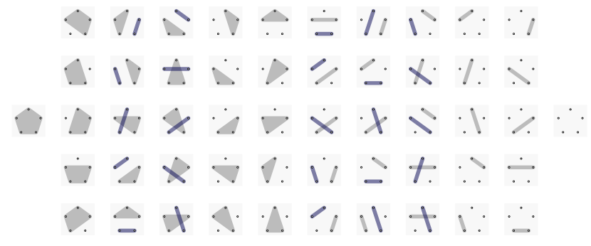
Figure 1: All 52 possible models given $K=5$, represented as partitions. Circles represent individual parameters and shaded regions indicate which parameters are equal.

The Stirling numbers and Bell numbers can be generalized to the $r$-Stirling [60] and $r$-Bell numbers [84], respectively. These generalizations help to construct conditional distributions, as we will see later. The $r$-Stirling numbers $\genfrac{\{}{\}}{0.0pt}{}{K}{j}_{r}$ give the number of partitions of size $j$ given $K+r$ groups such that the first $r$ parameters are all in distinct subsets. The $r$-Bell numbers give the total number of partitions given $K$ parameters where the first $r$ parameters are in distinct subsets. Specifically, we have:

$$\genfrac{\{}{\}}{0.0pt}{}{K}{j}_{r} =\sum_{i=0}^{K}\binom{K}{i}\genfrac{\{}{\}}{0.0pt}{}{i}{j}r^{K-i}$$ (3)

$$B_{K,\,r} =\sum_{i=0}^{K}\genfrac{\{}{\}}{0.0pt}{}{K+r}{i+r}_{r}\enspace.$$ (4)

Note that $\genfrac{\{}{\}}{0.0pt}{}{K}{j}_{1}=\genfrac{\{}{\}}{0.0pt}{}{K}{j}$ and that $B_{K,\,0}=B_{K}$. Both the $r$-Stirling and $r$-Bell numbers are defined through recurrence relations, although explicit expressions exist which are easier to compute for large values; see [60] and [84] for details.

2.3 Urn Schemes

We can represent the different partitions using an urn with $K$ different balls labeled 1 through $K$. For each parameter $\theta_{j}$, a ball $b_{j}$ is drawn from the urn with $b_{j}\in\{1,\ldots,K\}$. If two drawn balls are equal, $b_{i}=b_{j}$, then the two parameters are assigned to the same subset of the partition, that is, the two parameters $\theta_{i}$ and $\theta_{j}$ are equal if $b_{i}=b_{j}$. Note that different draws from an urn can represent the same partition. For example, the draws $(1,1,2)$ and $(3,3,1)$ both represent the partition $\{\{\theta_{1},\theta_{2}\},\{\theta_{3}\}\}$. The prior distributions introduced in the next sections assign probabilities to the unique partitions. Note that the prior probability of a particular draw can be obtained by dividing the probability of the corresponding partition by the total number of draws that correspond to that partition. The total number of draws that represent the same partition is given by $d!\binom{K}{d}$ where $d$ is the number of non-empty subsets of a particular draw.

Although the urn consists of $K$ different balls, the event of interest is whether the next ball drawn equals one of the balls already drawn — in other words, whether an equality or inequality is introduced. This event reduces the urn to a Pólya urn. All prior distributions discussed below are related to the Pólya urn. Specifically, the joint prior distribution on $(\theta_{1},\ldots,\theta_{K})$ is characterized by a (generalized) Pólya urn such that:

$$\theta_{K}\mid\theta_{1},\ldots,\theta_{K-1}\sim\begin{cases}\zeta_{j}&\text{with probability }P_{\pi}\\ \theta_{j}^{\star}&\text{with probability }1-P_{\pi}\enspace,\end{cases}$$ (5)

where $\zeta_{j}$ denotes a new value for $\theta_{K}$ (with $\theta_{1}=\zeta_{1}$) and $\theta_{j}^{\star}$ denotes a value equal to any previously observed value. We characterize the priors we discuss in the next section in terms of (5), which is known as a prediction rule [[, e.g.,]]ishwaran2001gibbs; in terms of the induced prior over partitions; and in terms of their penalty for multiplicity.

3 Methodology

Let $\vec{\theta^{\star}}=(\theta^{\star}_{1},\ldots,\theta^{\star}_{r})$ denote the vector of unique population parameters out of $\vec{\theta}=(\theta_{1},\ldots,\theta_{K})$, $\vec{\theta}_{-j}$ the vector of parameters without parameter $\theta_{j}$, and the number of repeats of $\theta^{\star}_{j}$ as $n^{\star}_{j}$. Let $\rho$ denote a partition and $|\rho|$ its size. For example, if $\rho=\{\{\theta_{1},\theta_{2}\},\{\theta_{3}\}\}$, then $|\rho|=2$. Similarly, for this example $\vec{\theta^{\star}}=(\theta^{\star}_{1},\theta^{\star}_{2})$ and $n^{\star}=(2,1)$. In the next sections, we discuss and contrast a number of priors.

3.1 Dirichlet Process Prior

The Dirichlet process (DP) is a distribution over distributions [69]. We say that $\mathcal{G}\sim\text{DP}(\alpha,\mathcal{K})$ is distributed according to a DP if its marginal distributions are Dirichlet distributed, where $\alpha$ is a concentration parameter and $\mathcal{K}$ is the base distribution, which will depend on the application; for details, see for example [96]. The DP can be understood as the infinite-dimensional generalization of the Dirichlet distribution, which makes it popular for mixture modeling [[, e.g.,]]rasmussen1999infinite. Our modeling approach is similar to mixture modeling, except that we do not cluster data but parameters — a cluster corresponds to a partition. The prediction rule of the DP is given by [[, e.g.,]]ishwaran2001gibbs, blackwell1973ferguson:

$$\theta_{j+1}\mid\theta_{1},\ldots,\theta_{j}\sim\begin{cases}\mathcal{K}&\text{with probability }\frac{\alpha}{\alpha+j-1}\\ \text{Categorical}\left(\theta_{1}^{\star},\ldots,\theta_{r}^{\star}\mid n^{\star}_{1},\ldots,n^{\star}_{r}\right)&\text{else}\enspace,\end{cases}$$ (6)

where $\alpha$ is the concentration parameter and the base distribution of the DP depends on the application (see Section 5). In other words, we draw a new value for $\theta_{j}$ from $\mathcal{K}$ with probability $\nicefrac{{\alpha}}{{\alpha+j-1}}$, or else set it to a previously observed value. The particular value $\theta^{\star}_{j}$ the parameter $\theta_{j}$ is set to is proportional to the number of times $\theta^{\star}_{j}$ was observed previously, given by $n^{\star}_{j}$, resulting in the well-known “rich get richer” property [[, e.g.,]]teh2010dirichlet.

The Dirichlet process implies a prior distribution over partitions. The prior on the partitions $\rho$ is:

$$\pi(\rho\mid\alpha)=\frac{\alpha^{|\rho|}\Gamma(\alpha)}{\Gamma(n+\alpha)}\prod_{c\in\rho}\Gamma(|c|)\enspace,$$ (7)

where $c$ is an element of $\rho$, and $|c|$ is its size. While the Dirichlet process features the infinite-dimensional object $\mathcal{K}$, the prior over partitions results from integrating it out. Hence the nonparametric model (in which the number of parameters is not fixed) implies a parametric model (in which the number of parameters is fixed) for the partitions, yielding what is sometimes referred to as a product partition model in the literature [[, e.g.,]]quintana2006predictive, quintana2003bayesian. This makes it usable for our purposes, where we have a fixed number of parameters.

The leftmost column in Figure 2 shows the DP prior over partitions (top) and number of inequalities (bottom) for different values of $\alpha$. Intuitively, one reasonable requirement for a prior in the context of penalizing multiplicity is to be monotonically decreasing in the number of partitions, which further implies a monotonically decreasing prior probability over the number of inequalities. This is the case for $\alpha=0.50$ (beige diamonds) as shown in the top and bottom panels, and indeed for any value $\alpha<1$. The value suggested by [72] creates a symmetric prior over the partitions (yellow suns), implying that the model with no inequalities is a priori as likely as the model with all inequalities (in the $K=5$ case, this yields $\alpha=2.213$). The prior with $\alpha=1$ (pink stars) results in a nonincreasing prior over the number of partitions, but in an increasing prior over the number of inequalities: the model with one inequality is more likely than the model with no inequalities.

As $\alpha\rightarrow 0$, the prior of the model with all $K-1$ equalities $\mathcal{M}_{0}$ (i.e., the null model) converges to one, while as $\alpha\rightarrow\infty$, the prior of the model with $K-1$ inequalities $\mathcal{M}_{B_{K}}$ (i.e., the full model) converges to one. For prior elicitation, [72] note that $\alpha$ is determined by specifying two of either $P(\mathcal{M}_{0})$, $P(\mathcal{M}_{B_{K}})$, or their ratio, since $P(\mathcal{M}_{0})=\nicefrac{{\alpha(K-1)!}}{{\prod_{j=1}^{K}(\alpha+j-1)}}$ and $P(\mathcal{M}_{B_{K}})=\nicefrac{{\alpha^{K}}}{{\prod_{j=1}^{K}(\alpha+j-1)}}$; see also Table 1.

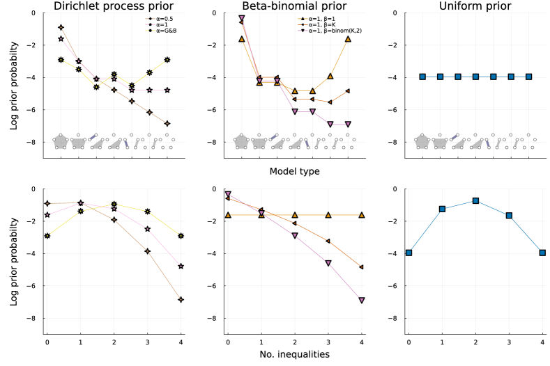
Figure 2: Top: Dirichlet process (left), beta-binomial (middle), and uniform prior (right) across distinct model types for $K=5$ groups and different prior parameters. Bottom: Same but for the number of inequalities across models.

	Dirichlet process prior	Beta-binomial prior	Uniform prior
Parameters	$\alpha$	$(\alpha=1,\beta)$	✗
Prior over partitions	$\frac{\alpha^{|\rho|}\Gamma(\alpha)}{\Gamma(n+\alpha)}\prod_{c\in\rho}\Gamma(|c|)$	$\binom{K-1}{|\rho|-1}\frac{\text{B}\left({|\rho|-1+\alpha},\ {K-|\rho|+\beta}\right)}{\text{B}\left({\alpha},\ {\beta}\right)\genfrac{\{}{\}}{0.0pt}{}{K}{|\rho|}}$	$\left(B_{K}\right)^{-1}$
Prior monotonically decreasing	$\alpha\leq 1$	$\beta\geq K$, $\beta\geq\binom{K}{2}$	✗
Prior probability of null model	$\nicefrac{{\alpha(K-1)!}}{{\prod_{j=1}^{K}(\alpha+j-1)}}$	$\nicefrac{{\text{B}\left({\alpha},\ {K-1+\beta}\right)}}{{\text{B}\left({\alpha},\ {\beta}\right)}}$	$\left(B_{K}\right)^{-1}$
Prior probability of full model	$\nicefrac{{\alpha^{K}}}{{\prod_{j=1}^{K}(\alpha+j-1)}}$	$\nicefrac{{\text{B}\left({K-1+\alpha},\ {\beta}\right)}}{{\text{B}\left({\alpha},\ {\beta}\right)}}$	$\left(B_{K}\right)^{-1}$
Prior probability of ratio (null / full)	$\nicefrac{{\alpha(K-1)!}}{{\alpha^{K}}}$	$\nicefrac{{\text{B}\left({\alpha},\ {K-1+\beta}\right)}}{{\text{B}\left({K-1+\alpha},\ {\beta}\right)}}$	$1$

Table 1: Characterizations of the different priors studied in this paper. Note: $\beta\geq K$ implies a prior decreasing in terms of the number of inequalities, but not in terms of the partitions. $\beta\geq\binom{K}{2}$ implies both.

3.2 Beta-binomial Prior

The beta-binomial model prior is a popular choice for stochastic search variable selection in linear regression [[]]george1993variable and Bayesian model averaging [[, e.g.,]]hinne2020conceptual, hoeting1999bayesian. It states that the prior probability of including $j$ predictors out of a total of $K$ predictors is given by:

$$\text{BB}\left(j\mid K,\ \alpha,\ \beta\right)=\binom{K}{j}\frac{\text{B}\left({j+\alpha},\ {K-j+\beta}\right)}{\text{B}\left({\alpha},\ {\beta}\right)}\enspace,$$ (8)

where $\alpha$ and $\beta$ are hyperparameters. The prior probability of a particular regression model is obtained by dividing by the number of ways $j$ out of $K$ predictors can be included: $\text{BB}\left(j\mid K,\ \alpha,\ \beta\right)/\binom{K}{j}$. The beta-binomial distribution introduces a penalty for including additional predictors and in that way introduces a correction for multiplicity [93, 94]. This beta-binomial prior over partitions can been seen as a special case of the hierarchical uniform prior where the distribution on the size of the partitions is a beta-binomial [62].

For the multiple comparison problem discussed in this paper, we consider the number of inequality constraints and use the beta-binomial prior to introduce a penalty for each additional inequality among the groups considered. For $K$ groups, there can be a maximum of $K-1$ inequalities, resulting in a $\text{BB}\left(i\mid K-1,\ \alpha,\ \beta\right)$ prior distribution over the number of included inequalities $i$ out of $K$ groups. To see how this translates to a prior over the partitions $\rho$, note that there is a one-to-many correspondence between the number of inequalities $i$ out of $K$ groups and the resulting partitions $\rho$. For example, having $i=1$ inequalities with $K=3$ groups is consistent with the partitions $\{\{\theta_{1},\theta_{2}\},\{\theta_{3}\}\}$, $\{\{\theta_{1},\theta_{3}\},\{\theta_{1}\}\}$, and $\{\{\theta_{2},\theta_{3}\},\{\theta_{1}\}\}$, all of which are of size $|\rho|=i+1$. The number of partitions of size $|\rho|$ is given, as discussed above, by the Stirling number $\genfrac{\{}{\}}{0.0pt}{}{K}{|\rho|}$. For the assignment of the prior probability, it is only the size of the partition (the number of inequalities) that counts. With these observations in hand, we arrive at the following (adjusted) beta-binomial prior distribution over partitions $\rho$:

$$\pi(\rho\mid K,\alpha,\beta)=\binom{K-1}{|\rho|-1}\frac{\text{B}\left({|\rho|-1+\alpha},\ {K-|\rho|+\beta}\right)}{\text{B}\left({\alpha},\ {\beta}\right)\genfrac{\{}{\}}{0.0pt}{}{K}{|\rho|}}\enspace.$$ (9)

The prediction rule of the beta-binomial prior is given by:

$$\theta_{j+1}\mid\theta_{1},\ldots,\theta_{j}\sim\begin{cases}\mathcal{K}&\text{with probability }P_{\pi}\\ \text{Categorical}\left(\theta_{1}^{\star},\ldots,\theta_{r}^{\star}\mid 1,\ldots,1\right)&\text{else}\enspace.\end{cases}\enspace,$$ (10)

where

$$P_{\pi} =\frac{\sum_{\begin{subarray}{c}\rho\in\mathrm{P}\\ \theta_{j}\notin\vec{\theta}_{-j}\subseteq\rho\end{subarray}}\text{BB}\left(\rho\mid K,\ \alpha,\ \beta\right)}{\sum_{\begin{subarray}{c}\rho\in\mathrm{P}\\ \theta_{j}\notin\vec{\theta}_{-j}\subseteq\rho\end{subarray}}\text{BB}\left(\rho\mid K,\ \alpha,\ \beta\right)+\sum_{\begin{subarray}{c}\rho\in\mathrm{P}\\ \theta_{j}\in\vec{\theta}_{-j}\subseteq\rho\end{subarray}}\text{BB}\left(\rho\mid K,\ \alpha,\ \beta\right)}\enspace,$$ (11)

and where $$\mathrm{P} \theta_{j} \vec{\theta}_{-j} \vec{\theta}_{-j} r$$ denotes the set of all possible partitions. In essence, Equation (11) takes the probability of all possible partitions where is distinct from , conditional on being a subset of the considered partition. The sum over all possible partitions can be simplified using the -Stirling numbers:

$$P_{\pi} =\frac{\sum_{i=1}^{K}\text{BB}\left(i\mid K,\ \alpha,\ \beta\right)\genfrac{\{}{\}}{0.0pt}{}{K-j+r+1}{i}_{r+1}}{r\sum_{j=i}^{K}\text{BB}\left(i\mid K,\ \alpha,\ \beta\right)\genfrac{\{}{\}}{0.0pt}{}{K-j+r}{i}_{r}+\sum_{i=1}^{K}\text{BB}\left(i\mid K,\ \alpha,\ \beta\right)\genfrac{\{}{\}}{0.0pt}{}{K-j+r+1}{i}_{r+1}}\enspace,$$ (12)

where $r$ is number of unique parameters in $\vec{\theta}$, that is, the size of the partition.

The beta-binomial prior on the partitions and the induced prior on the number of inequalities are shown for different parameterizations in the middle column in Figure 2. For $\alpha=\beta=1$, the beta-binomial distribution over the partitions has a characteristic U-shape (orange triangles). This prior specification in turn implies a uniform prior on the number of inequalities. We follow [98] who, in the context of regression, suggested to set $\alpha=1$ as a default so that the distribution over model size (here the number of inequalities) is nonincreasing, and to scale $\beta=\lambda K$ with the number of groups to force the prior to be monotonically decreasing, with a default of $\lambda=1$ [98]. This is illustrated as the red line (leftward pointing triangles) in Figure 2 using $\beta=5$. In the multiple comparison case, we additionally investigate $\beta={K\choose 2}$, which implies that the prior on the number of inequalities of individual models is nonincreasing, see Appendix B. The purple line (upside-down triangles) in Figure 2 shows a decreasing prior for $\beta={5\choose 2}=10$. This prior assigns the least mass to models with an increasing number of inequalities compared to all others beta-binomial priors.

Figure 2 shows that the DP prior makes a distinction that the beta-binomial is, by design, not making: while the beta-binomial prior assigns the same prior mass to partitions with the same number of (in)equalities, the DP prior assigns more mass to the partition with the larger cluster. For example, the beta-binomial does not distinguish between $\{\{\theta_{1},\theta_{2},\theta_{3}\},\{\theta_{4}\},\{\theta_{5}\}\}$ and $\{\{\theta_{1},\theta_{2}\},\{\theta_{3},\theta_{4}\},\{\theta_{5}\}\}$, while the DP assigns more mass to the former (see Figure 2). We return to this distinction in the discussion.

Lastly, note that for the beta-binomial prior we have that $P(\mathcal{M}_{0})=\nicefrac{{\text{B}\left({\alpha},\ {K-1+\beta}\right)}}{{\text{B}\left({\alpha},\ {\beta}\right)}}$ and $P(\mathcal{M}_{B_{K}})=\nicefrac{{\text{B}\left({K-1+\alpha},\ {\beta}\right)}}{{\text{B}\left({\alpha},\ {\beta}\right)}}$. Fixing $\alpha=1$, we have that as $\beta\rightarrow\infty$, the prior of the model with all $K-1$ equalities $\mathcal{M}_{0}$ converges to one, while as $\beta\rightarrow 0$, the prior of the model with $K-1$ inequalities $\mathcal{M}_{B_{K}}$ converges to one; see also Table 1. As with the Dirichlet process prior discussed above, one can use these relations in prior elicitation.

3.3 Uniform Prior

For completeness, we give a prior that is uniform over the space of partitions. The probability mass function is straightforward. All valid configurations of size $K$ have probability $\nicefrac{{1}}{{B_{K}}}$. The prediction rule of the uniform prior is given by:

$$\theta_{j+1}\mid\theta_{1},\ldots,\theta_{j}\sim\begin{cases}\mathcal{K}&\text{with probability }P_{\pi_{U}}\\ \text{Categorical}\left(\theta_{1}^{\star},\ldots,\theta_{r}^{\star}\mid 1,\ldots,1\right)&\text{else}\enspace,\end{cases}$$ (13)

where

$$P_{\pi_{U}} =\frac{B_{K-j+1,\,r+1}}{B_{K-j+1,\,r+1}+rB_{K-j+1,\,r}}$$ (14)

Here, $B_{K-j+1,\,r+1}$ counts the number of models where $\theta_{j+1}\notin\left(\theta_{1}^{\star},\ldots,\theta_{r}^{\star}\right)$ conditional on $\theta_{1},\ldots,\theta_{j}$ being assigned to $r$ distinct subsets. Complementarily, $B_{K-j+1,\,r}$ counts the number of models where $\theta_{j+1}\in\left(\theta_{1}^{\star},\ldots,\theta_{r}^{\star}\right)$ conditional on $\theta_{1},\ldots,\theta_{j}$ being assigned to $r$ distinct subsets, which is multiplied by $r$ as there are $r$ subsets that $\theta_{j+1}$ could be assigned to. Under this uniform prior, all partitions $\rho$ are equally likely, as can be seen in the top right panel in Figure 2. Note that this uniform prior induces a non-uniform prior on the number of inequalities, as shown in the bottom right panel.

3.4 Posterior Model Consistency

Model selection consistency is a key desiderata that a good Bayes factor should fulfill [[, e.g.,]]bayarri2012criteria, ly2016harold, consonni2018prior. In the situation of multiple models, the notion of pairwise model selection consistency needs to be extended. This extension is referred to as posterior model selection consistency. Posterior model consistency in a model class $\mathfrak{M}$ is the convergence to one, in probability, of the posterior probabilities to the true model [[, e.g.,]]casella2009consistency, moreno2015posterior. Let $\mathcal{M}_{j}\in\mathfrak{M}$ be the model that instantiates the hypothesis $\mathcal{H}_{j}$ that specifies the (in)equalities among $K$ groups. The posterior probability of $\mathcal{M}_{j}$ is given by:

$$p(\mathcal{M}_{j}\mid\mathcal{D}) =\frac{p(\mathcal{D}\mid\mathcal{M}_{j})\pi(\mathcal{M}_{j})}{\sum_{i=0}^{B_{K}}p(\mathcal{D}\mid\mathcal{M}_{i})\pi(\mathcal{M}_{i})}=\frac{\text{BF}_{j0}\pi(\mathcal{M}_{j})}{\sum_{i=0}^{B_{K}}\text{BF}_{i0}\pi(\mathcal{M}_{i})}\enspace.$$ (15)

It follows that if the Bayes factor is model selection consistent, posterior model consistency holds [[, see also]Theorem 1]moreno2015posterior — unless the prior assigns zero mass to the true model. This is not the case for any of the priors discussed above, and hence whether posterior model consistency holds depends solely on the priors on the parameters within models. In other words, if one uses priors that lead to model selection consistent Bayes factors [[, e.g.,]]bayarri2012criteria, ly2016harold, dablander2020default, as we do in Sections 4 and 5, then using the beta-binomial, Dirichlet process, or uniform prior outlined above leads to a procedure that is posterior model selection consistent.

3.5 Stochastic Search Method

When the number of groups is small and the computation of Bayes factors is swift, one can directly compute the Bayes factors for all hypotheses. Using the priors we outlined above, one can then obtain posterior distributions over hypotheses that incorporate the desired multiplicity adjustment. The number of (in)equalities grows extremely quickly with the number of groups, however, and for larger number of groups one must rely on stochastic search methods. Moreover, while directly computing the Bayes factors results in posterior distributions over hypotheses, it does not yield posterior distributions over parameters. We therefore set up a stochastic search method that yields both, allowing researchers to incorporate uncertainty across hypotheses through model averaging [[, e.g.,]]hinne2020conceptual, hoeting1999bayesian.

Our method is implemented in the programming language Julia [56]. First, we implemented the prior distributions in Julia. Next, we used the library Turing.jl, which is designed for general-purpose probabilistic programming [70]. Turing enabled us to directly reuse the distributions defined in Julia code and also provided a multitude of options for composing different MCMC samplers. We set up a Gibbs sampler that explored the posterior space in two steps. The first step used Turing’s built-in Hamiltonian Monte Carlo methods for sampling from the posterior distributions of the continuous parameters. In all models discussed here, all parameters are continuous except for the partitions. The second step used a custom Gibbs algorithm for sampling from the posterior distribution over partitions. The partitions were represented as a vector of integers denoted $\vec{\gamma}$ that indicate partition membership. By partition membership, we mean that two parameters $\theta_{i}$ and $\theta_{j}$ are in the same partition if and only if $\gamma_{i}=\gamma_{j}$. For example, $\{\{\theta_{1}\},\{\theta_{2},\theta_{3}\}\}$ could be represented by $(1,2,2)$ but also by $(3,1,1)$. We first explain the remainder of the sampling scheme and motivate the duplicate representations in the next paragraph. The number of possible duplicate representations in $\vec{\gamma}$ for one partition is straightforward to compute, and the prior over $\vec{\gamma}$ is obtained by taking the prior over the partitions and dividing uniformly over duplicate representations. Next, we sample each element of $\vec{\gamma}$ conditional on the other elements. Since the partition membership is discrete, we enumerate all possible values and draw from the resulting categorical distribution. Sampling individual elements of $\vec{\gamma}$ from the conditional distributions rather than the joint distribution reduces the complexity from $\mathcal{O}(B_{K})$ to $\mathcal{O}(K^{2})$.

Although the duplicate representations of $\vec{\gamma}$ for one partition introduce some additional computational cost, they facilitate exploration of the posterior space. For example, if we had used a one-to-one mapping from partitions to $\vec{\gamma}$, then updating the first membership in $(1,2,2)$ to $(2,2,2)$ would not be a valid configuration, as this should be represented by $(1,1,1)$. However, a transition from $(1,2,2)$ to $(1,1,1)$ requires updating two parameters and is therefore less likely to occur. Nevertheless, on the level of partitions, it makes sense to propose a move from $\{\{\theta_{1}\},\{\theta_{2},\theta_{3}\}\}$ to $\{\{\theta_{1},\theta_{2},\theta_{3}\}\}$.

4 Investigating Multiplicity Adjustment

In this section, we investigate the differences between the above priors in more detail and compare them to the method proposed by [97] and an uncorrected approach using pairwise Bayes factors. In Section 4.1, we use a small simulation study to illustrate the implications of multiplicity adjustment. In Section 4.2, we present the results of a more extensive simulation study.

4.1 Illustrating Multiplicity Adjustment

Here we illustrate the different multiplicity penalties that the different priors impose using a small simulation study. We simulate data from a one-way ANOVA model and analyze it using the specification by [92]. The ANOVA model extended with a prior over partitions is given by:

$$Y_{ij} \sim\mathcal{N}\left(\mu+\sigma\theta_{j},1\right)$$

$$\mu \propto 1$$

$$\sigma^{2} \propto 1/\sigma^{2}$$

$$g \sim\mathcal{IG}\left(\nicefrac{{1}}{{2}},\nicefrac{{1}}{{2}}\right)$$

$$\vec{\theta}^{u} \sim\mathcal{N}_{K-1}\left(0,g\right)$$

$$\vec{\theta}^{c} \leftarrow\mathbf{Q}\vec{\theta}^{u}$$

$$\theta_{j} \leftarrow\text{mean of elements of }\theta^{c}\text{ in the same partition }$$

$$\rho \sim\pi_{\rho}(.)\enspace.$$ (16)

The data follow a Gaussian distribution with a grand mean $\mu$ and a group-specific offset $\theta_{j}$. The offsets sum to zero to avoid identification constraints. This is achieved by projecting $\vec{\theta}^{u}$ from a $K-1$ dimensional space onto a $K$ dimensional space using the matrix $\mathbf{Q}$, which consists of the first $K-1$ columns of an eigendecomposition of a degenerate covariance matrix as defined in [92]. Next, the elements of $\vec{\theta}^{c}$ within the same partition are averaged to obtain $\theta_{j}$. The unconstrained offsets $\vec{\theta}^{u}$ are assigned a $g$ prior where $g$ itself is assigned an inverse gamma prior with shape and scale equal to $\nicefrac{{1}}{{2}}$ [81]. Note that the model reduces to the approach of [92] whenever the partition indicates that all elements are distinct.

We simulated from the null model, which assumes that all the groups are equal, and from the full model, which assumes that all groups are unequal, drawing 100 observations per group and varying the number of groups $K\in[2,3,\dots,10]$, repeating each combination 100 times. In the full model, the means were of increasing size with successive differences of $0.20$. For the analysis we considered six priors: the Dirichlet process prior with $\alpha\in\{0.50,1\}$ and $\alpha$ set adaptively to have equal prior mass assigned to the model with all equalities and the model with all inequalities (i.e., $p(\mathcal{H}_{0})=p(\mathcal{H}_{1})$), as done by [72]; the beta-binomial prior with $\alpha=1$ and $\beta\in\{1,K,{K\choose 2}\}$; and the uniform prior. We also included the prior adjustment method proposed by [97] and an uncorrected method using pairwise Bayes factors. We used our methodology as described in Section 3.5, drawing 12,000 MCMC samples and discarding the first 2,000 as a burn-in.

To assess how well the respective priors adjust for multiplicity, we calculated how frequently the posterior probability that any two groups differ is larger than 0.50, using the null model as data-generating model. Similarly, to assess how well the respective priors are capable of detecting true differences, we calculated how frequently the posterior probability that any two groups do not differ is larger than 0.50, using the full model as data-generating model.

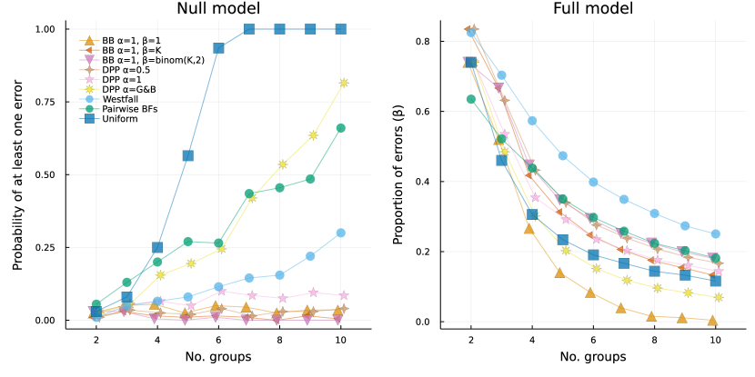
Figure 3: Left: Probability of making at least one false claim about a difference between two groups when there is none. Right: Proportion of falsely claiming no difference between two groups when there is one.

The left panel in Figure 3 shows that using a uniform prior (blue squares) very quickly leads to false positives as the number of groups increases. This is not surprising: the uniform prior assigns each model the same prior mass, hence diminishing the plausibility assigned to $\mathcal{H}_{0}$ dramatically as $K$ increases, thus increasing the probability of an error. The Dirichlet process prior which assigns equal mass to the full and the null model (yellow suns), as suggested by [72], performs better than the uniform prior but still does not provide adequate error control. It performs roughly as poorly as the method which simply computes pairwise Bayesian $t$-tests (green circles). The correction proposed by [97] performs much better (light blue circles) but still leads to a relatively high probability of making at least one error as the number of groups increases. The DP prior with $\alpha=1$ (pink stars) performs better, with the DP prior with $\alpha=0.50$ (beige diamonds) and the set of beta-binomial priors providing good error control.

The right panel in Figure 3 shows that the beta-binomial prior with $\alpha=\beta=1$ leads to the lowest proportion of falsely claiming no difference between two groups, followed by the Dirichlet process prior for which $p(\mathcal{H}_{0})=p(\mathcal{H}_{1})$ and the uniform prior. The method proposed by [97] performs worst, followed by the beta-binomial prior with $\alpha=1$ and $\beta={K\choose 2}$ and the DP prior with $\alpha=0.50$. The performance of the uncorrected pairwise Bayes factor approach is somewhere in the middle. Note that all approaches perform better as the group size increases, but this is due to our simulation design: each additional group exhibits a mean larger than the previous one by $0.20$ and adds $n$ more observations, which makes falsely claiming no difference less likely with an increasing number of groups. Instead of looking at absolute error, we therefore focus on the relative ordering of the priors. Overall, we conclude that not adjusting for multiple comparisons — either by using a uniform prior or by using pairwise Bayes factors — naturally leads to the worst performance and that the method by [97] is overly conservative and does not provide adequate error control with an increasing number of groups. In the next section, we report on a more extensive simulation study to further disentangle the differences between the multiple comparison methods.

4.2 Simulation Study

In the previous section, we illustrated the importance of adjusting the prior model probabilities in reducing the familywise error rate when all groups are equal. Here we explore the multiplicity adjustment of the different methods in a more exhaustive simulation study. We used the same ANOVA model as in the previous section and varied the total number of groups $K\in\{5,9\}$ and the sample size per group $n\in\{50,100,250,500\}$. In addition, we varied the true number of equalities to be $\{0\%,25\%,50\%,75\%,100\%\}$. For $K=5$, there are 4 possible (in)equalities which resulted in models that have either 0, 1, 2, 3, or 4 equalities. For $K=9$, there are 8 possible (in)equalities, resulting in 0, 2, 4, 6, or 8 equalities in the true model. Given the number of equalities, we sampled a particular partition uniformly from all possible partitions with that amount of equalities and used this model to simulate data. Each unique combination was repeated 100 times and each generated data set was analyzed with the same prior specifications as above. We assessed the familywise error control as well as statistical power. The results for K = 5 and K = 9 were similar. Therefore, we focus on the $K=5$ in the main text and discuss the $K=9$ case in Appendix C.

Note that the hierarchical approach has an additional source of $\alpha$ error in contrast to pairwise comparisons when there are more than 0 inequalities because it imposes transitivity. For example, imagine that the true model postulates that $\theta_{1}=\theta_{2}=\theta_{3}\neq\theta_{4}$. However, the sample means are (by random sampling) $\bar{x}_{1}=0.1,\bar{x}_{2}=0.2,\bar{x}_{3}=0.3,\bar{x}_{4}=0.35$. The hierarchical approach would find that $\theta_{3}=\theta_{4}$, but not that $\theta_{1}=\theta_{3}$ since that also implies $\theta_{1}=\theta_{4}$. Therefore, the model $\theta_{1}=\theta_{2}=\theta_{3}\neq\theta_{4}$ and even the equality $\theta_{1}=\theta_{2}$ are not retrieved. In contrast, the pairwise methods violate transitivity as they only look at two pairs at the time and will happily suggest that $\theta_{1}=\theta_{2}$, $\theta_{2}=\theta_{3}$, and $\theta_{3}=\theta_{4}$ while simultaneously suggesting that $\theta_{1}\neq\theta_{4}$.

4.2.1 Familywise Error Rate

Figure 4 shows the probability of at least one error for different methods across the number of inequalities in the true model and sample sizes. The top left panel shows that the uniform prior (blue squares), the pairwise Bayes factors (green circles), the Dirichlet process prior with ($p(\mathcal{H}_{0})=p(\mathcal{H}_{1})$) (yellow stars), and the method proposed by [97] (light blue circles) perform worst and that the other Dirichlet process and beta-binomial priors provide adequate error control. This mirrors the results above, which is natural since this part of the simulation is a special case for $K=5$. Increasing the number of inequalities to 1 (top right) and 2 (bottom left), we find that the pairwise Bayes factors, the method by [97], and the uniform improve in performance. This is likely due to the fact that, with more inequalities, there are simply less opportunities to incorrectly claim that two population means are different. In contrast, the performance of the other methods decreases when there is at least one inequality; it is difficult to disentangle a trend with increasing inequalities.

The rightmost panel in Figure 4 shows the results averaged over the number of inequalities in the true model. We find that the method by [97] shows the strongest familywise error control, closely followed by the the beta-binomial priors with $\beta=K$ and $\beta={K\choose 2}$ and the DP prior with $\alpha=0.50$. The pairwise Bayes factors perform similar to the Dirichlet process prior with $\alpha=1$, with the beta-binomial prior with $\beta=1$, the symmetric DP prior, and the uniform prior performing worst. The differences between the methods become less pronounced with increasing sample size since the data starts to dominate the prior.

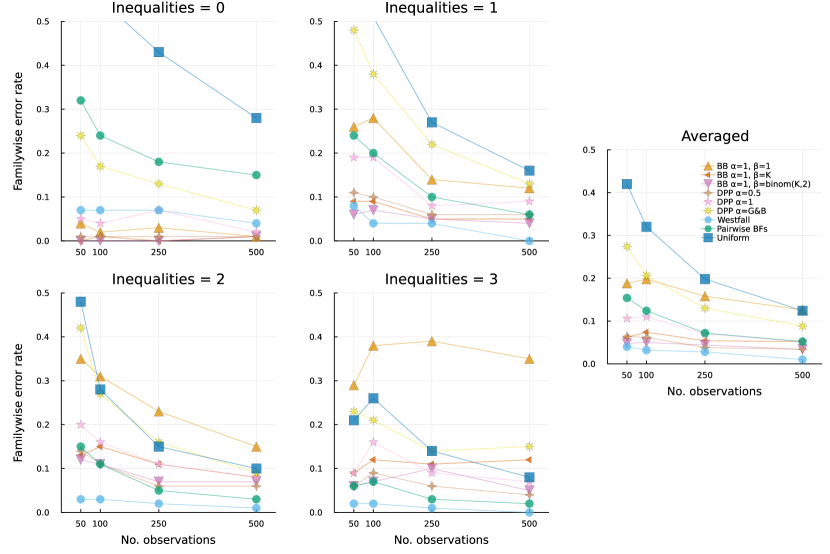
Figure 4: Familywise error rate across priors and sample sizes under a model with 0 (top left), 1 (top right), 2 (bottom left), and 3 (bottom right) true inequalities for $K=5$ groups. The rightmost panel shows the average familywise error rate across inequalities.

4.2.2 Statistical Power

Figure 5 shows the proportion of falsely claiming a difference between two groups when there is none for different methods across the number of equalities in the true model and sample sizes. The top left panel shows that the beta-binomial prior with $\beta=1$ performs best and the method proposed by [97] performs worst, again mirroring the results of the small simulation study above. Increasing the number of equalities in the true model, we find that the performance of virtually all methods decreases except for the uniform prior, which shows a slight increase, especially for large sample sizes. This overall decrease in performance is likely due to the fact that the average pairwise difference between groups decreases with the number of equalities. To illustrate, note that the model with no equalities for $K=4$ groups has population means $\vec{\mu}=\{-0.30,-0.10,0.10,0.30\}$, which yields pairwise differences $[0.20,0.20,0.20,0.40,0.40,0.60]$ with an average of $0.33$. In contrast, including one equality results in $\vec{\mu}=\{-0.25,-0.05,0.15,0.15\}$, yielding pairwise differences of $[0.20,0.20,0.20,0.40,0.40]$ with an average of $0.28$.

The rightmost panel in Figure 5 shows the results averaged over the number of equalities in the true model. We find that the method by [97] is highly conservative, trading off the strong familywise error control with an increase in the proportion of false negatives. Similarly, the priors that performed worst with respect to familywise error control — the uniform, symmetric DP, and beta-binomial prior with $\beta=1$ — perform best here. The other DP and beta-binomial priors as well as the pairwise Bayes factors are somewhere in between those two extremes. Note that again the differences between the methods become less pronounced with increasing sample size.

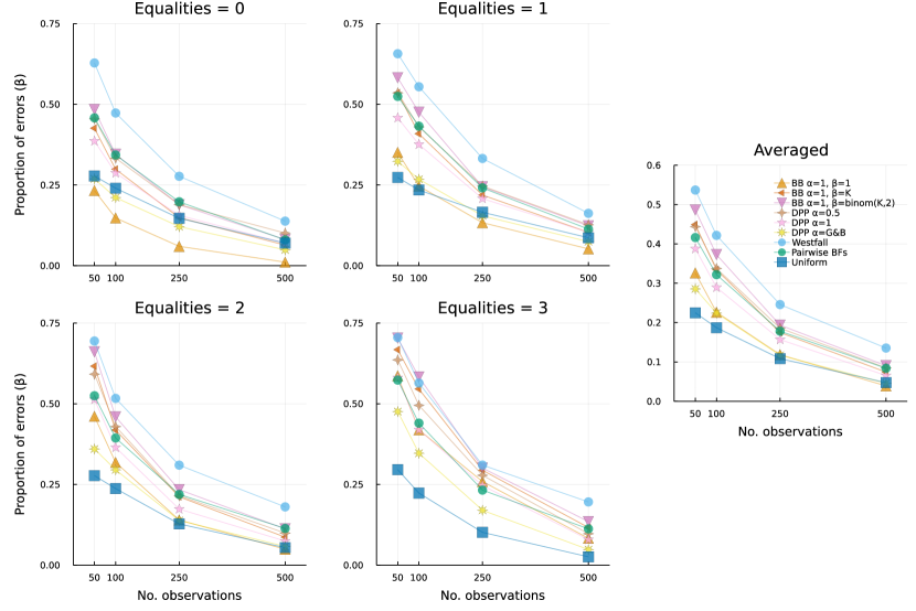
Figure 5: Proportion of falsely claiming a difference between two groups when there is none across priors and sample sizes under a model with 0 (top left), 1 (top right), 2 (bottom left), and 3 (bottom right) true inequalities for $K=5$ groups. The rightmost panel shows the average error rate across inequalities.

4.2.3 Simulation Discussion

Our results show that no single method dominates all others. While the beta-binomial prior with $\beta=1$ performed best in our initial simulation study described in Section 4.1, including models beyond the null and full model showed that this prior performed considerably worse in those settings. The beta-binomial prior with $\beta=K$, $\beta={K\choose 2}$, and the DP prior with $\alpha=0.50$ perform very similarly overall. In the next section, we focus on the beta-binomial prior with $\beta=K$ and apply our method to two examples.

5 Applications

In this section, we apply the beta-binomial setup to two examples: testing the (in)equality of proportions and variances, respectively. We have developed a generic Julia package called EqualitySampler that utilizes the probabilistic programming framework Turing to allow the user to adjust for multiplicity as proposed in this paper.

5.1 Testing Proportions

[87] investigated a sample of 30,717 articles published between 1985 and 2013 in eight major psychology journals for statistical reporting errors. Our question here is: Which journals make the same amount of errors, and which make more errors? We answer the question using the following model specification. For journal $j$, denote the number of statistical errors found as $e_{j}$ and the number of statistical tests analyzed as $n_{j}$. We assume that underlying each proportion there is a latent true chance of making an error, $\theta_{j}$. Thus, we modeled the data as independent binomials, that is, $e_{j}\sim\mathrm{Binomial}\left(\theta_{j},n_{j}\right)$. Next, we specify a hierarchical level over the partitions to assess for which journals the chances of making an error are equal. This leads to the following model specification:

$$e_{j} \sim\mathrm{Binomial}\left(\theta_{j},n_{j}\right)$$

$$\theta^{u}_{j} \sim\text{Beta}(1,1)$$

$$\theta_{j} \leftarrow\text{mean of elements of }\theta^{u}_{j}\text{ in the same partition }$$

$$\rho \sim\text{beta-binomial}(1,8)\enspace.$$ (17)

The unconstrained chances $\theta^{u}_{j}$ are assigned beta priors from which — together with the partitions — the possibly constrained chances are created. Two chances $\theta_{i}$ and $\theta_{j}$ are equal if and only if their indices appear in the same partition $\{i,j\}\subseteq\rho_{k}$ for some $k$. Note that the model reduces to the full model of independent binomials whenever the partitions state that all elements in $\vec{\theta}$ are distinct. We use a beta-binomial prior with $\alpha=1$ and $\beta=8$. The top left panel in Figure 6 shows the posterior distributions for the underlying error chance for each journal under a model that assumes that they are all different.

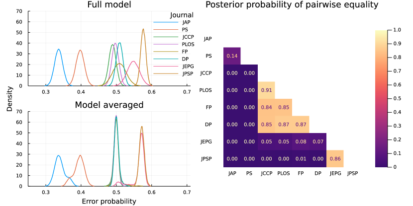
Figure 6: Left: Posterior means of the full model where all proportions are assumed to be different (top) and posterior means when averaging over all models using a beta-binomial($\alpha=1$, $\beta=8$) prior (bottom). Right: Posterior probabilities for pairwise equality across all journals. The abbreviations stand for: Journal of Applied Psychology (JAP), Psychological Science (PS), Journal of Consulting and Clinical Psychology (JCCP), Public Library of Science (PLOS), Developmental Psychology (DP), Journal of Experimental Psychology: General (JEPG), and Journal of Personality and Social Psychology (JPSP).

We can see that the posterior distributions for JCCP (green), PLOS (purple), DP (turquoise), and FP (beige) are very close to each other, with FP showing more pronounced uncertainty. The panel below shows the model-averaged posterior distributions, clearly demonstrating a shrinkage effect. The error chances for JAP and PS are pulled toward each other, with JCCP, PLOS, DP, and FP being shrunk towards each other almost completely, similarly to JEPG and JPSP. The right panel in Figure 6 gives the posterior distributions for pairwise equality across all journals, reflecting the two main clusters in the model-averaged density plot on the left.

5.2 Testing Standard Deviations

[59] studied whether men and women differ in the variability of personality traits. Here we focus on five personality traits (agreeableness, extraversion, openness, conscientiousness, neuroticism) rated by participants’ peers in an Estonian sample consisting of $n_{1}=969$ women and $n_{2}=716$ men. Our goal is to assess which personality traits across the sexes can be assumed equal in terms of their variability. This example shows how our methodology can be used to test group differences while taking the multivariate dependency of the outcome measure into account. We build on the parameterization proposed by [65], who developed a default Bayes factor test for testing the (in)equality of variances. Let $\vec{y}_{1}$ and $\vec{y}_{2}$ denote the five-element vectors of observed data for men and women, respectively, and $K=10$ be the total number of variables. For each sex $k\in\{1,2\}$, we have:

$$\vec{Y}_{k} \sim\mathcal{N}\left(\vec{\mu}_{k},\Sigma_{k}\right)$$

$$\vec{\mu}_{k} \propto\vec{1}$$

$$\Sigma_{k} =\text{diag}(\vec{\sigma}_{k})\,\Omega_{k}\,\text{diag}(\vec{\sigma}_{k})$$

$$\Omega_{k} \sim\text{LKJ}(1)\enspace,$$

where LKJ refers to the Lewandowski-Kurowicka-Joe prior [80]. To test the equality of variances both between and across groups, we define the ten-variable standard deviation vector $\vec{\sigma}=[\vec{\sigma}_{1},\vec{\sigma}_{2}]$ with $\bar{\sigma}$ denoting the average standard deviation. Following [65], we write $\sigma_{j}=\left(K\vartheta_{j}\bar{\sigma}\right)^{-1}$, where $\vartheta_{j}=\nicefrac{{\sigma_{j}}}{{\sum_{j=1}^{K}\sigma_{j}}}$ is the relative standard deviation and $\vartheta_{K}=1-\sum_{j=1}^{K-1}\vartheta_{j}$. To complete the model specification, we write:

$$\sigma_{j} =\left(K\vartheta_{j}\bar{\sigma_{j}}\right)^{-1}$$

$$\bar{\sigma}_{j} \propto\bar{\sigma}_{j}^{-1}$$

$$\vartheta_{j} \leftarrow\text{mean of elements of }\vartheta^{u}\text{ in the same partition }$$

$$\vec{\vartheta}^{u} \sim\text{Dirichlet}(1,\ldots,1)$$

$$\rho \sim\text{beta-binomial}(1,10)\enspace.$$ (18)

Two standard deviations $\sigma_{i}$ and $\sigma_{j}$ are equal if and only if their indices appear in the same partition $\{i,j\}\subseteq\rho_{k}$ for some $k$. When the partition states that all standard deviations are distinct we recover the full model. The top left panel of Figure 7 shows the posterior distributions under the full model that assumes all standard deviations are different.

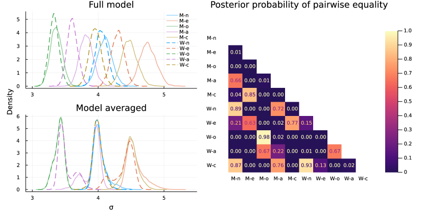
Figure 7: Left: Posterior means of the full model where all standard deviations are assumed to be different (top) and posterior means when averaging across all models using a beta-binomial($\alpha$ = 1, $\beta$ = 10) prior (bottom). Right: Posterior probabilities for pairwise equality across all personality traits. In the abbreviations the first letter stands for men (m) or women (w). The second letter stands for neuroticism (n), extraversion (e), openness (o), agreeableness (a), and conscientiousness (c).

While all posterior distributions lie close to each other, the standard deviations of openness for men and women overlap particularly much. The bottom panel shows the model-averaged posterior distributions, which again demonstrate a shrinkage effect. The right panel of Figure 7 shows the posterior probability of pairwise equality across all personality traits for men and women. It appears that there are three clusters: (1) men–openness, women–openness, and women–agreeableness; (2) men–neuroticism, women–neuroticism, women–conscientiousness, and men–agreeableness; (3) men–conscientiousness, men–extraversion, and women–extraversion. However, for the personality traits women–agreeableness, men–agreeableness, and women–extraversion, the evidence is not overwhelming, as indicated by the bimodality in the model-averaged posterior distributions.

6 Discussion

Testing the (in)equality between groups while adjusting for multiple comparisons is a core challenge in many applied settings. In this paper, we have proposed a flexible class of beta-binomial priors to penalize multiplicity and make inferences over all possible (in)equalities in relatively general settings. We compared the beta-binomial priors to a Dirichlet process prior suggested by [72], to a uniform prior, to the method proposed by [97], and to an uncorrected method based on pairwise Bayes factors. We also illustrated our method, which is freely available in the Julia package EqualitySampler, on two examples.

We found that a beta-binomial prior with $\alpha=1$ and $\beta\in\{K,{K\choose 2}\}$ as well as a Dirichlet process prior with $\alpha<1$ adequately control the familywise error rate, while a uniform prior and using only pairwise Bayes factors, unsurprisingly, do not. We also found that the method proposed by [97] compares favorably in terms of error control but not in terms of power. While we have focused on a posterior probability threshold of $0.50$ (i.e., a Bayes factor of 1), other thresholds will naturally impact the trade-off between the two types of errors. Importantly, and in contrast to conventional adjustments for multiple comparisons [[, e.g.,]]westfall1997bayesian, jeffreys1961theory, specifying a prior over the partitions allows inferences over all possible (in)equalities. This means that researchers can use the methods we provide to assess not only the probability of pairwise (in)equalities — as is common in standard post-hoc tests for, say, ANOVA — but in fact can make probabilistic statements over any set of (in)equalities they wish to assess. Similarly, the outlined approach also allows for model-averaging, which as we have seen in the applications yields shrinkage of the groups towards each other.

Ideally, inferences are drawn using the model-averaged posterior distribution. However, sometimes there is a need to select a single model among all candidate models. An obvious choice is the highest posterior density model (HPM). However, as the number of groups increases, it becomes increasingly less likely that a stochastic search algorithm visits the HPM and the sampling uncertainty for the posterior probability of individual models also increases. An alternative that is often used in regression is the median probability model (MPM), which is obtained by retaining all predictors with a posterior probability larger than $\nicefrac{{1}}{{2}}$ [51, 50]. In the context of multiple comparison adjustment, there is the additional constraint that one wants to select a model that is also a valid partition, and the MPM may not necessarily satisfy this constraint. We present an example where the MPM proposes a model that is not a partition and suggests two possible solutions in Appendix D.

As with any statistical method, there are a number of points to keep in mind. While we suggest default values of $\alpha=1$ and $\beta=K$ for the beta-binomial prior and $\alpha\leq 1$ for the DP prior, researchers may wish to use a more informed prior specification. Values for the prior parameters can be elicited by specifying model priors for two out of the following: the prior on the null model, on the full model, or their ratio. The resulting probabilities for equality among pairs of parameters can then be assessed by the elicitee. As [[]p. 1132]gopalan1998bayesian note, if these do not adequately represent the elicitee’s beliefs, and if the elicitee cannot make adjustments of the prior on the null model and the full model to resolve this circumstance, then the Dirichlet process prior is not appropriate. The beta-binomial prior is more flexible in this regard, because it has an additional parameter that can be varied to accommodate prior beliefs (see Table 1). If the elicitee’s beliefs cannot be accommodated even with two parameters, then in principle it is also possible to substitute the beta-binomial with a categorical distribution that assigns custom probabilities to partitions of the same size. However, if partitions of the same size should be assigned different prior probabilities, then the beta-binomial prior — and the more general categorical distribution — is inappropriate. Importantly, the beta-binomial prior differs from the DP prior in that it assigns models with the same number of partitions the same prior probability, while the DP prior assigns more mass to the model with the larger cluster. It is not obvious which of the two behaviors is more desirable, and it may well depend on the problem under study. Researchers using the methods we have made available should keep this difference in mind, although the extent to which it matters in practice remains to be seen.

There are some practical limitations of our implementation that we leave for future work. We currently do not allow for factorial designs, for example, for which dummy or contrast coding is more natural. The key challenge there is to specify the prior in such a way that it reflects the structure of the experimental design. For the present, we believe that the Bayesian approach outlined in this paper can help improve the inferences of applied researchers who wish to compare multiple groups.

Author Contributions.

DvB and FD proposed the study and refined it in numerous discussions. DvB implemented the method and created the Julia package. FD and DvB designed the simulation study. DvB conducted the simulation study and analyzed the data with the help of FD. FD and DvB wrote the manuscript. All authors read and approved the submitted version of the paper. They also declare that there were no conflicts of interest.

Appendix A Example Code

The code below illustrates the proportion example in Section 5.1. To install the package enter the Pkg REPL by typing ] and install the package with add EqualitySampler. Alternatively, the package can be installed by importing the Pkg package: import Pkg; Pkg.add(EqualitySampler).

using EqualitySampler, EqualitySampler.Simulationsimport DataFrames      as DF,       LinearAlgebra   as LA,       NamedArrays     as NA,       CSV,       AbstractMCMC# working directory is assumed to be the root of the GitHub repositoryjournal_data = DF.DataFrame(CSV.File(joinpath("simulations", "demos","data", "journal_data.csv")))# Kn_journals = size(journal_data, 1)# no of observed errorserrors = round.(Int, journal_data.n .* journal_data.errors)# no of possible errorsobservations = journal_data.n# run 4 chains in parallel with 15_000 iterations per chain of which# the first 5_000 are discardedmcmc_settings = MCMCSettings(;iterations = 15_000, burnin = 5_000,                             chains = 4, parallel = AbstractMCMC.MCMCThreads)# nothing indicates no equality sampling is done and samples are drawn from# the full modelchn_full = proportion_test(errors, observations, nothing;                           mcmc_settings = mcmc_settings)# use a BetaBinomial(1, k) over the partitionspartition_prior = BetaBinomialPartitionDistribution(n_journals, 1, n_journals)chn_eqs  = proportion_test(errors, observations, partition_prior;                           mcmc_settings = mcmc_settings)# chn_full and chn_eqs contain posterior samples# the posterior probability that two journals are equaleqs_mat = compute_post_prob_eq(chn_eqs)NA.NamedArray(  LA.UnitLowerTriangular(round.(eqs_mat; digits = 3)),  (journal_data.journal, journal_data.journal))# 8×8 Named LinearAlgebra.UnitLowerTriangular{Float64, Matrix{Float64}}#  A \ B |  "JAP"    "PS"  "JCCP"  "PLOS"    "FP"    "DP"  "JEPG"  "JPSP"# -------+---------------------------------------------------------------# "JAP"  |    1.0     0.0     0.0     0.0     0.0     0.0     0.0     0.0# "PS"   |  0.134     1.0     0.0     0.0     0.0     0.0     0.0     0.0# "JCCP" |    0.0     0.0     1.0     0.0     0.0     0.0     0.0     0.0# "PLOS" |    0.0     0.0   0.909     1.0     0.0     0.0     0.0     0.0# "FP"   |    0.0     0.0   0.861    0.87     1.0     0.0     0.0     0.0# "DP"   |    0.0     0.0   0.864   0.886   0.881     1.0     0.0     0.0# "JEPG" |    0.0     0.0   0.059   0.063    0.09    0.08     1.0     0.0# "JPSP" |    0.0     0.0     0.0     0.0   0.005     0.0   0.852     1.0# The table above is approximately equal to the right panel of Figure 6.

Appendix B Beta-binomial Prior with Decreasing Prior Model Odds

Proposition 1.

The prior density of the beta-binomial distribution over partitions is decreasing for $\alpha=1$ and $\beta\geq\binom{K}{2}$, and strictly decreasing for $\alpha=1$ and $\beta>\binom{K}{2}$.

Proof.

The prior density of the Beta-binomial over partitions is given by:

$$\pi\left(\rho\mid K,\alpha,\beta\right)=\binom{K-1}{|\rho|-1}\frac{\text{B}\left({|\rho|-1+\alpha},\ {K-|\rho|+\beta}\right)}{\text{B}\left({\alpha},\ {\beta}\right)\genfrac{\{}{\}}{0.0pt}{}{K}{|\rho|}}\enspace.$$

To examine the ratio of two consecutive model sizes we evaluate the ratio of the prior for partitions $\rho$ and $q$ with $|q|=|\rho|+1$:

$$\frac{\pi\left(\rho\mid K,\,\alpha,\,\beta\right)}{\pi\left(q\mid K,\,\alpha,\,\beta\right)} =\frac{\binom{K-1}{|\rho|-1}}{\binom{K-1}{|\rho|}}\,\frac{\text{B}\left({|\rho|-1+\alpha},\ {K-|\rho|+\beta}\right)}{\text{B}\left({|\rho|+\alpha},\ {K-|\rho|-1+\beta}\right)}\,\frac{\genfrac{\{}{\}}{0.0pt}{}{K}{|\rho|+1}}{\genfrac{\{}{\}}{0.0pt}{}{K}{|\rho|}},$$ (19)

$$=\frac{|\rho|}{K-|\rho|}\,\frac{\beta+K-|\rho|-1}{\alpha+|\rho|-1}\,\frac{\genfrac{\{}{\}}{0.0pt}{}{K}{|\rho|+1}}{\genfrac{\{}{\}}{0.0pt}{}{K}{|\rho|}}.$$ (20)

Using the recurrence relation of the Stirling numbers $\genfrac{\{}{\}}{0.0pt}{}{n+1}{k}=k\genfrac{\{}{\}}{0.0pt}{}{n}{k}+\genfrac{\{}{\}}{0.0pt}{}{n}{k-1}$, the ratio $\nicefrac{{\genfrac{\{}{\}}{0.0pt}{}{K}{|\rho|+1}}}{{\genfrac{\{}{\}}{0.0pt}{}{K}{|\rho|}}}$ is equivalent to $\nicefrac{{\genfrac{\{}{\}}{0.0pt}{}{K+1}{|\rho|+1}}}{{\genfrac{\{}{\}}{0.0pt}{}{K}{|\rho|+1}}}-(|\rho|+1)$. This ratio of Stirling numbers was studied by [54] and their property 2 provides this inequality

$$\frac{\genfrac{\{}{\}}{0.0pt}{}{K+1}{|\rho|+1}}{\genfrac{\{}{\}}{0.0pt}{}{K}{|\rho|+1}}-|\rho|-1\geq\frac{\genfrac{\{}{\}}{0.0pt}{}{K+1}{|\rho|}}{\genfrac{\{}{\}}{0.0pt}{}{K}{|\rho|}}-|\rho|.$$

It follows that the ratio in Equation (19) is maximal at $|\rho|=K-1$ and has value $\binom{K}{2}$. Next, we fix $\alpha=1$ and solve $\nicefrac{{\pi\left(K\mid K-1,\,1,\,\beta\right)}}{{\pi\left(K\mid K,\,1,\,\beta\right)}}=1$ for $\beta$ which yields $\beta=\binom{K}{2}$. Thus $\beta\geq\binom{K}{2}$ implies $\pi\left(j+1\mid K,\,1,\,\beta\right)\geq\pi\left(j\mid K,\,1,\,\beta\right)$ (resp. $\beta>\binom{K}{2}$ implies $\pi\left(j+1\mid K,\,1,\,\beta\right)>\pi\left(j\mid K,\,1,\,\beta\right)$). ∎

Appendix C Simulation Results for $K=9$

Here we present the extended simulation results for the $K=9$ group case. Figure 8 mirrors the results for the $K=9$ case, namely that the pairwise Bayes factors, the method proposed by [97], and the uniform prior generally increase in performance as the number of inequalities increase, while the other priors generally decrease in performance. Averaging over the settings, we again find that the beta-binomial prior with $\beta=1$, the uniform prior, and the symmetric DP prior exhibit the worst error control, with the method proposed by [97] performing best, closely followed by the beta-binomial prior with $\beta={K\choose 2}$ and the DP prior with $\alpha=0.50$.

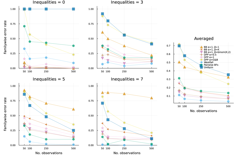
Figure 8: Familywise error rate across priors and sample sizes under a model with 0 (top left), 3 (top right), 5 (bottom left), and 7 (bottom right) true inequalities for $K=9$ groups. The rightmost panel shows the average familywise error rate across inequalities.

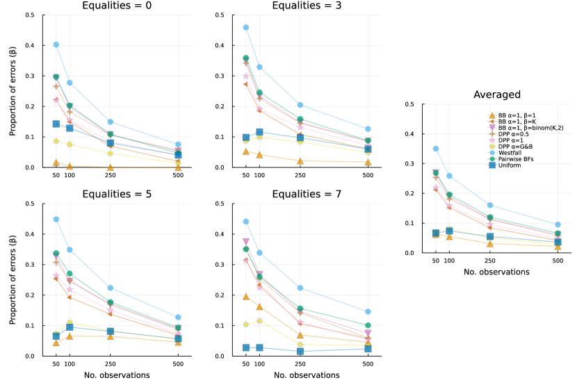
Figure 9: Proportion of falsely claiming a difference between two groups when there is none across priors and sample sizes under a model with 0 (top left), 3 (top right), 5 (bottom left), and 7 (bottom right) true inequalities for $K=9$ groups. The rightmost panel shows the average error rate across inequalities.

Appendix D Selecting the Optimal Model

The median probability model (MPM) is not guaranteed to select a valid partition. To see this, suppose we have obtained an equal number of posterior samples for the partitions $\{\{\theta_{1},\theta_{2}\},\{\theta_{3},\theta_{4}\}\}$, $\{\{\theta_{1}\},\{\theta_{2},\theta_{3},\theta_{4}\}\}$, and $\{\{\theta_{1},\theta_{2},\theta_{3}\},\{\theta_{4}\}\}$. Table 2 shows the resulting model-averaged probabilities of equality.

Table 2: An example of model-averaged posterior probabilities where the median probability model is not a valid partition.

	$\theta_{1}$	$\theta_{2}$	$\theta_{3}$
$\theta_{2}$	$\nicefrac{{2}}{{3}}$
$\theta_{3}$	$\nicefrac{{1}}{{3}}$	$\nicefrac{{2}}{{3}}$
$\theta_{4}$	$\nicefrac{{0}}{{3}}$	$\nicefrac{{1}}{{3}}$	$\nicefrac{{2}}{{3}}$

The posterior probabilities larger than $\nicefrac{{1}}{{2}}$ are $p(\theta_{1}=\theta_{2})=\nicefrac{{2}}{{3}}$, $p(\theta_{2}=\theta_{3})=\nicefrac{{2}}{{3}}$, and $p(\theta_{3}=\theta_{4})=\nicefrac{{2}}{{3}}$. Transitivity would imply that $\theta_{1}=\theta_{4}$, but we have that $p(\theta_{1}=\theta_{4})=\nicefrac{{0}}{{3}}<\nicefrac{{1}}{{2}}$. The MPM therefore does not yield a valid partition.

We propose two solutions that are inspired by the median probability model. The first solution is to find a partition that is closest to the model-averaged posterior probabilities of equality. That is, we want a partition $\rho$ that minimizes

$$\sum_{i<j}\left(I(\rho\Rightarrow\theta_{i}=\theta_{j})-p(\theta_{i}=\theta_{j}\mid\vec{y})\right)^{2}\enspace,$$ (21)

where $I(\rho\Rightarrow\theta_{i}=\theta_{j})$ is 1 if the partition $\rho$ implies that $\theta_{i}$ equals $\theta_{j}$ and 0 otherwise. For the example in Table 2, this solution suggests that the optimal partition is $\{\{\theta_{1},\theta_{2}\},\{\theta_{3},\theta_{4}\}\}$. The second approach is similar to the first, but rather than minimizing the distance to the probabilities of equality, we minimize the distance to the model-averaged posterior distributions on the level of the parameters. We do so by finding a partition $\rho$ that minimizes $d(p(\theta\mid\vec{y},\rho),p(\theta\mid\vec{y}))$, where $d$ is a distance function, $p(\theta\mid\vec{y},\rho)$ is the posterior distribution conditional on partition $\rho$, and $p(\theta\mid\vec{y})$ is the model averaged posterior. In principle, any distance function can be used, but in regression contexts it is common to use the squared distance between the mean of the distributions. The first solution is a discrete optimization problem that is relatively easy to carry out using existing software for integer programming [[, e.g., JuMP;]]lubin2023jump. The second solution is more complex to carry out because it may be necessary to resample from the posterior distribution for a given partition, but also closer to the optimality condition for the MPM of [[]Eq. 16]barbieri2004optimal.

References

- [1] Maria M Barbieri, James O Berger, Edward I George and Veronika Ročková “The median probability model and correlated variables” In Bayesian Analysis 16.4 International Society for Bayesian Analysis, 2021, pp. 1085–1112
- [2] Maria Maddalena Barbieri and James O. Berger “Optimal predictive model selection” In The Annals of Statistics 32.3 Institute of Mathematical Statistics, 2004, pp. 870–897
- [3] Maria J Bayarri, James O Berger, Anabel Forte and G García-Donato “Criteria for Bayesian model choice with application to variable selection” In The Annals of Statistics 40.3 Institute of Mathematical Statistics, 2012, pp. 1550–1577
- [4] Yoav Benjamini and Henry Braun “John W. Tukey’s contributions to multiple comparisons” In The Annals of Statistics 30.6 Institute of Mathematical Statistics, 2002, pp. 1576–1594
- [5] Sven Berg “Some properties and applications of a ratio of Stirling numbers of the second kind” In Scandinavian Journal of Statistics JSTOR, 1975, pp. 91–94
- [6] Donald A Berry and Yosef Hochberg “Bayesian perspectives on multiple comparisons” In Journal of Statistical Planning and Inference 82.1-2 Elsevier, 1999, pp. 215–227
- [7] Jeff Bezanson, Alan Edelman, Stefan Karpinski and Viral B Shah “Julia: A fresh approach to numerical computing” In SIAM Review 59.1 SIAM, 2017, pp. 65–98
- [8] David Blackwell and James B MacQueen “Ferguson distributions via Pólya urn schemes” In The Annals of Statistics 1.2 Institute of Mathematical Statistics, 1973, pp. 353–355
- [9] Małgorzata Bogdan, Jayanta K Ghosh and Surya T Tokdar “A comparison of the Benjamini-Hochberg procedure with some Bayesian rules for multiple testing” In arXiv preprint arXiv:0805.2479, 2008
- [10] Peter Borkenau et al. “Sex differences in variability in personality: A study in four samples” In Journal of Personality 81.1 Wiley Online Library, 2013, pp. 49–60
- [11] Andrei Z Broder “The -Stirling numbers” In Discrete Mathematics 49.3 Elsevier, 1984, pp. 241–259
- [12] George Casella, F Javier Girón, M Lina Martínez and Elias Moreno “Consistency of Bayesian procedures for variable selection” In The Annals of Statistics 37.3 Institute of Mathematical Statistics, 2009, pp. 1207–1228
- [13] George Casella, Elías Moreno and F Javier Girón “Cluster analysis, model selection, and prior distributions on models” In Bayesian Analysis 9, 2014
- [14] Sean Chang and James O Berger “Frequentist properties of Bayesian multiplicity control for multiple testing of normal means” In Sankhya A 82 Springer, 2020, pp. 310–329
- [15] Guido Consonni, Dimitris Fouskakis, Brunero Liseo and Ioannis Ntzoufras “Prior distributions for objective Bayesian analysis” In Bayesian Analysis 13.2 International Society for Bayesian Analysis, 2018, pp. 627–679
- [16] Fabian Dablander, Don Bergh, Alexander Ly and Eric-Jan Wagenmakers “Default Bayes Factors for Testing the (In) equality of Several Population Variances” In Bayesian Analysis, 2023, pp. 1–25
- [17] David B Dahl and Michael A Newton “Multiple hypothesis testing by clustering treatment effects” In Journal of the American Statistical Association 102.478 Taylor & Francis, 2007, pp. 517–526
- [18] Tim Jong “A Bayesian approach to the correction for multiplicity”, 2019 DOI: 10.31234/osf.io/s56mk
- [19] Francesco Denti et al. “Two-group Poisson-Dirichlet mixtures for multiple testing” In Biometrics 77.2 Wiley Online Library, 2021, pp. 622–633
- [20] Thomas S Ferguson “A Bayesian analysis of some nonparametric problems” In The Annals of Statistics JSTOR, 1973, pp. 209–230
- [21] Hong Ge, Kai Xu and Zoubin Ghahramani “Turing: a language for flexible probabilistic inference” In International Conference on Artificial Intelligence and Statistics, AISTATS 2018, 9-11 April 2018, Playa Blanca, Lanzarote, Canary Islands, Spain, 2018, pp. 1682–1690
- [22] Edward I George and Robert E McCulloch “Variable selection via Gibbs sampling” In Journal of the American Statistical Association 88.423 Taylor & Francis, 1993, pp. 881–889
- [23] Ramanan Gopalan and Donald A Berry “Bayesian multiple comparisons using Dirichlet process priors” In Journal of the American Statistical Association 93.443 Taylor & Francis Group, 1998, pp. 1130–1139
- [24] Mengye Guo and Daniel F Heitjan “Multiplicity-calibrated Bayesian hypothesis tests” In Biostatistics 11.3 Oxford University Press, 2010, pp. 473–483
- [25] Max Hinne, Quentin F Gronau, Don Bergh and Eric-Jan Wagenmakers “A conceptual introduction to Bayesian model averaging” In Advances in Methods and Practices in Psychological Science 3.2 SAGE Publications Sage CA: Los Angeles, CA, 2020, pp. 200–215
- [26] Jennifer A Hoeting, David Madigan, Adrian E Raftery and Chris T Volinsky “Bayesian model averaging: a tutorial” In Statistical Science JSTOR, 1999, pp. 382–401
- [27] Hemant Ishwaran and Lancelot F James “Gibbs sampling methods for stick-breaking priors” In Journal of the American Statistical Association 96.453 Taylor & Francis, 2001, pp. 161–173
- [28] Harold Jeffreys “Theory of Probability (3rd Ed.)” Oxford, UK: Oxford University Press, 1961
- [29] Robert E Kass and Adrian E Raftery “Bayes factors” In Journal of the American Statistical Association 90.430 Taylor & Francis, 1995, pp. 773–795
- [30] Sinae Kim, David B Dahl and Marina Vannucci “Spiked Dirichlet Process Prior for Bayesian Multiple Hypothesis Testing in Random Effects Models” In Bayesian Analysis 4.4, 2009, pp. 707–732
- [31] Daniel Lewandowski, Dorota Kurowicka and Harry Joe “Generating random correlation matrices based on vines and extended onion method” In Journal of Multivariate Analysis 100.9 Elsevier, 2009, pp. 1989–2001
- [32] Feng Liang et al. “Mixtures of g priors for Bayesian variable selection” In Journal of the American Statistical Association 103.481 Taylor & Francis, 2008, pp. 410–423
- [33] Miles Lubin et al. “JuMP 1.0: recent improvements to a modeling language for mathematical optimization” In Mathematical Programming Computation Springer, 2023, pp. 1–9
- [34] Alexander Ly, Josine Verhagen and Eric-Jan Wagenmakers “Harold Jeffreys’s default Bayes factor hypothesis tests: Explanation, extension, and application in psychology” In Journal of Mathematical Psychology 72 Elsevier, 2016, pp. 19–32
- [35] István Mezo “The -Bell numbers” In Journal of Integer Sequences 14.1 Citeseer, 2011, pp. 1–14
- [36] Jeffrey W Miller and Matthew T Harrison “A simple example of Dirichlet process mixture inconsistency for the number of components” In Proceedings of the 26th International Conference on Neural Information Processing Systems-Volume 1, 2013, pp. 199–206
- [37] Elías Moreno, Javier Girón and George Casella “Posterior model consistency in variable selection as the model dimension grows” In Statistical Science 30.2 Institute of Mathematical Statistics, 2015, pp. 228–241
- [38] Michèle B Nuijten et al. “The prevalence of statistical reporting errors in psychology (1985–2013)” In Behavior Research Methods 48.4 Springer, 2016, pp. 1205–1226
- [39] Fernando A Quintana “A predictive view of Bayesian clustering” In Journal of Statistical Planning and Inference 136.8 Elsevier, 2006, pp. 2407–2429
- [40] Fernando A Quintana and Pilar L Iglesias “Bayesian clustering and product partition models” In Journal of the Royal Statistical Society: Series B (Statistical Methodology) 65.2 Wiley Online Library, 2003, pp. 557–574
- [41] CV Rao and U Swarupchand “Multiple comparison procedures-a note and a bibliography” In Journal of Statistics 16.1 Citeseer, 2009, pp. 66–109
- [42] Carl Edward Rasmussen “The infinite Gaussian mixture model” In NIPS 12, 1999, pp. 554–560
- [43] Jeffrey N Rouder, Richard D Morey, Paul L Speckman and Jordan M Province “Default Bayes factors for ANOVA designs” In Journal of Mathematical Psychology 56.5 Elsevier, 2012, pp. 356–374
- [44] James G Scott and James O Berger “An exploration of aspects of Bayesian multiple testing” In Journal of Statistical Planning and Inference 136.7 Elsevier, 2006, pp. 2144–2162
- [45] James G Scott and James O Berger “Bayes and empirical-Bayes multiplicity adjustment in the variable-selection problem” In The Annals of Statistics JSTOR, 2010, pp. 2587–2619
- [46] Stan Development Team “Stan Modeling Language Users Guide and Reference Manual, 2_30.”, 2022 URL: https://mc-stan.org
- [47] Yee Whye Teh “Dirichlet Process.” In Encyclopedia of Machine Learning 1063 Citeseer, 2010, pp. 280–287
- [48] Peter H Westfall, Wesley O Johnson and Jessica M Utts “A Bayesian perspective on the Bonferroni adjustment” In Biometrika 84.2 Oxford University Press, 1997, pp. 419–427
- [49] Melanie A Wilson et al. “Bayesian model search and multilevel inference for SNP association studies” In The Annals of Applied Statistics 4.3 NIH Public Access, 2010, pp. 1342–1364
- [50] Maria M Barbieri, James O Berger, Edward I George and Veronika Ročková “The median probability model and correlated variables” In Bayesian Analysis 16.4 International Society for Bayesian Analysis, 2021, pp. 1085–1112
- [51] Maria Maddalena Barbieri and James O. Berger “Optimal predictive model selection” In The Annals of Statistics 32.3 Institute of Mathematical Statistics, 2004, pp. 870–897
- [52] Maria J Bayarri, James O Berger, Anabel Forte and G García-Donato “Criteria for Bayesian model choice with application to variable selection” In The Annals of Statistics 40.3 Institute of Mathematical Statistics, 2012, pp. 1550–1577
- [53] Yoav Benjamini and Henry Braun “John W. Tukey’s contributions to multiple comparisons” In The Annals of Statistics 30.6 Institute of Mathematical Statistics, 2002, pp. 1576–1594
- [54] Sven Berg “Some properties and applications of a ratio of Stirling numbers of the second kind” In Scandinavian Journal of Statistics JSTOR, 1975, pp. 91–94
- [55] Donald A Berry and Yosef Hochberg “Bayesian perspectives on multiple comparisons” In Journal of Statistical Planning and Inference 82.1-2 Elsevier, 1999, pp. 215–227
- [56] Jeff Bezanson, Alan Edelman, Stefan Karpinski and Viral B Shah “Julia: A fresh approach to numerical computing” In SIAM Review 59.1 SIAM, 2017, pp. 65–98
- [57] David Blackwell and James B MacQueen “Ferguson distributions via Pólya urn schemes” In The Annals of Statistics 1.2 Institute of Mathematical Statistics, 1973, pp. 353–355
- [58] Małgorzata Bogdan, Jayanta K Ghosh and Surya T Tokdar “A comparison of the Benjamini-Hochberg procedure with some Bayesian rules for multiple testing” In arXiv preprint arXiv:0805.2479, 2008
- [59] Peter Borkenau et al. “Sex differences in variability in personality: A study in four samples” In Journal of Personality 81.1 Wiley Online Library, 2013, pp. 49–60
- [60] Andrei Z Broder “The -Stirling numbers” In Discrete Mathematics 49.3 Elsevier, 1984, pp. 241–259
- [61] George Casella, F Javier Girón, M Lina Martínez and Elias Moreno “Consistency of Bayesian procedures for variable selection” In The Annals of Statistics 37.3 Institute of Mathematical Statistics, 2009, pp. 1207–1228
- [62] George Casella, Elías Moreno and F Javier Girón “Cluster analysis, model selection, and prior distributions on models” In Bayesian Analysis 9, 2014
- [63] Sean Chang and James O Berger “Frequentist properties of Bayesian multiplicity control for multiple testing of normal means” In Sankhya A 82 Springer, 2020, pp. 310–329
- [64] Guido Consonni, Dimitris Fouskakis, Brunero Liseo and Ioannis Ntzoufras “Prior distributions for objective Bayesian analysis” In Bayesian Analysis 13.2 International Society for Bayesian Analysis, 2018, pp. 627–679
- [65] Fabian Dablander, Don Bergh, Alexander Ly and Eric-Jan Wagenmakers “Default Bayes Factors for Testing the (In) equality of Several Population Variances” In Bayesian Analysis, 2023, pp. 1–25
- [66] David B Dahl and Michael A Newton “Multiple hypothesis testing by clustering treatment effects” In Journal of the American Statistical Association 102.478 Taylor & Francis, 2007, pp. 517–526
- [67] Tim Jong “A Bayesian approach to the correction for multiplicity”, 2019 DOI: 10.31234/osf.io/s56mk
- [68] Francesco Denti et al. “Two-group Poisson-Dirichlet mixtures for multiple testing” In Biometrics 77.2 Wiley Online Library, 2021, pp. 622–633
- [69] Thomas S Ferguson “A Bayesian analysis of some nonparametric problems” In The Annals of Statistics JSTOR, 1973, pp. 209–230
- [70] Hong Ge, Kai Xu and Zoubin Ghahramani “Turing: a language for flexible probabilistic inference” In International Conference on Artificial Intelligence and Statistics, AISTATS 2018, 9-11 April 2018, Playa Blanca, Lanzarote, Canary Islands, Spain, 2018, pp. 1682–1690
- [71] Edward I George and Robert E McCulloch “Variable selection via Gibbs sampling” In Journal of the American Statistical Association 88.423 Taylor & Francis, 1993, pp. 881–889
- [72] Ramanan Gopalan and Donald A Berry “Bayesian multiple comparisons using Dirichlet process priors” In Journal of the American Statistical Association 93.443 Taylor & Francis Group, 1998, pp. 1130–1139
- [73] Mengye Guo and Daniel F Heitjan “Multiplicity-calibrated Bayesian hypothesis tests” In Biostatistics 11.3 Oxford University Press, 2010, pp. 473–483
- [74] Max Hinne, Quentin F Gronau, Don Bergh and Eric-Jan Wagenmakers “A conceptual introduction to Bayesian model averaging” In Advances in Methods and Practices in Psychological Science 3.2 SAGE Publications Sage CA: Los Angeles, CA, 2020, pp. 200–215
- [75] Jennifer A Hoeting, David Madigan, Adrian E Raftery and Chris T Volinsky “Bayesian model averaging: a tutorial” In Statistical Science JSTOR, 1999, pp. 382–401
- [76] Hemant Ishwaran and Lancelot F James “Gibbs sampling methods for stick-breaking priors” In Journal of the American Statistical Association 96.453 Taylor & Francis, 2001, pp. 161–173
- [77] Harold Jeffreys “Theory of Probability (3rd Ed.)” Oxford, UK: Oxford University Press, 1961
- [78] Robert E Kass and Adrian E Raftery “Bayes factors” In Journal of the American Statistical Association 90.430 Taylor & Francis, 1995, pp. 773–795
- [79] Sinae Kim, David B Dahl and Marina Vannucci “Spiked Dirichlet Process Prior for Bayesian Multiple Hypothesis Testing in Random Effects Models” In Bayesian Analysis 4.4, 2009, pp. 707–732
- [80] Daniel Lewandowski, Dorota Kurowicka and Harry Joe “Generating random correlation matrices based on vines and extended onion method” In Journal of Multivariate Analysis 100.9 Elsevier, 2009, pp. 1989–2001
- [81] Feng Liang et al. “Mixtures of g priors for Bayesian variable selection” In Journal of the American Statistical Association 103.481 Taylor & Francis, 2008, pp. 410–423
- [82] Miles Lubin et al. “JuMP 1.0: recent improvements to a modeling language for mathematical optimization” In Mathematical Programming Computation Springer, 2023, pp. 1–9
- [83] Alexander Ly, Josine Verhagen and Eric-Jan Wagenmakers “Harold Jeffreys’s default Bayes factor hypothesis tests: Explanation, extension, and application in psychology” In Journal of Mathematical Psychology 72 Elsevier, 2016, pp. 19–32
- [84] István Mezo “The -Bell numbers” In Journal of Integer Sequences 14.1 Citeseer, 2011, pp. 1–14
- [85] Jeffrey W Miller and Matthew T Harrison “A simple example of Dirichlet process mixture inconsistency for the number of components” In Proceedings of the 26th International Conference on Neural Information Processing Systems-Volume 1, 2013, pp. 199–206
- [86] Elías Moreno, Javier Girón and George Casella “Posterior model consistency in variable selection as the model dimension grows” In Statistical Science 30.2 Institute of Mathematical Statistics, 2015, pp. 228–241
- [87] Michèle B Nuijten et al. “The prevalence of statistical reporting errors in psychology (1985–2013)” In Behavior Research Methods 48.4 Springer, 2016, pp. 1205–1226
- [88] Fernando A Quintana “A predictive view of Bayesian clustering” In Journal of Statistical Planning and Inference 136.8 Elsevier, 2006, pp. 2407–2429
- [89] Fernando A Quintana and Pilar L Iglesias “Bayesian clustering and product partition models” In Journal of the Royal Statistical Society: Series B (Statistical Methodology) 65.2 Wiley Online Library, 2003, pp. 557–574
- [90] CV Rao and U Swarupchand “Multiple comparison procedures-a note and a bibliography” In Journal of Statistics 16.1 Citeseer, 2009, pp. 66–109
- [91] Carl Edward Rasmussen “The infinite Gaussian mixture model” In NIPS 12, 1999, pp. 554–560
- [92] Jeffrey N Rouder, Richard D Morey, Paul L Speckman and Jordan M Province “Default Bayes factors for ANOVA designs” In Journal of Mathematical Psychology 56.5 Elsevier, 2012, pp. 356–374
- [93] James G Scott and James O Berger “An exploration of aspects of Bayesian multiple testing” In Journal of Statistical Planning and Inference 136.7 Elsevier, 2006, pp. 2144–2162
- [94] James G Scott and James O Berger “Bayes and empirical-Bayes multiplicity adjustment in the variable-selection problem” In The Annals of Statistics JSTOR, 2010, pp. 2587–2619
- [95] Stan Development Team “Stan Modeling Language Users Guide and Reference Manual, 2_30.”, 2022 URL: https://mc-stan.org
- [96] Yee Whye Teh “Dirichlet Process.” In Encyclopedia of Machine Learning 1063 Citeseer, 2010, pp. 280–287
- [97] Peter H Westfall, Wesley O Johnson and Jessica M Utts “A Bayesian perspective on the Bonferroni adjustment” In Biometrika 84.2 Oxford University Press, 1997, pp. 419–427
- [98] Melanie A Wilson et al. “Bayesian model search and multilevel inference for SNP association studies” In The Annals of Applied Statistics 4.3 NIH Public Access, 2010, pp. 1342–1364