Dark Energy Star in Gravity’s Rainbow

Abstract

The concept of dark energy can be a candidate for preventing the gravitational collapse of compact objects to singularities. According to the usefulness of gravity’s rainbow in UV completion of general relativity (by providing a new description of spacetime), it can be an excellent option to study the behavior of compact objects near phase transition regions. In this work, we obtain a modified Tolman-Openheimer-Volkof (TOV) equation for anisotropic dark energy as a fluid by solving the field equations in gravity’s rainbow. Next, to compare the results with general relativity, we use a generalized Tolman-Matese-Whitman mass function to determine the physical quantities such as energy density, radial pressure, transverse pressure, gravity profile, and anisotropy factor of the dark energy star. We evaluate the junction condition and investigate the dynamical stability of dark energy star thin shell in gravity’s rainbow. We also study the energy conditions for the interior region of this star. We show that the coefficients of gravity’s rainbow can significantly affect this non-singular compact object and modify the model near the phase transition region.

I Introduction

The existence of a strange cosmic fluid known as dark energy (DE) with the negative pressure, describes the universe’s accelerating expansion, requiring special consideration in other structures, including compact objects. In these cases, it also seems that using other modified gravity is a solution to the problem of quantum-mechanical incompatibility and general relativity. With the link between physical concepts on the demand of the general relativity, quantum mechanics and condensed matter physics by Chapline Chapline , a new era in the development of alternative theories of black holes was formed. It may also be possible at the surface of a black hole (event horizon) a behavior similar to that of a Bose gas. In the sense that it is possible that the surface of a black hole is a result of a quantum phase transition.

One of the alternative candidates to the black hole theory is gravastar. The concept of gravastar was first introduced by Mazur and Mottola MazurM2004 . They introduced a compact object with three regions and different space-times; the interior vacuum region, which is related to the cosmological constant, the middle region, which is a shell with a finite thickness, and the equation of state of a perfect fluid governs it, and also the exterior region, which contains a true vacuum, and the pressure in it is zero MazurM2004 . The advantage of this model is that there is no singularity at the center of this compact object, and there is also no horizon MazurM2004 . Many studies have been done on gravastar. A $5-$layer model similar to the introduced gravastar in Ref. MazurM2004 plus a junction interface in the middle region was investigated by Visser and Wiltshire VisserW2004 . For the first time, gravastars with anisotropic pressures were studied by Cattoen et al. Cattoen2005 . They showed that the Tolman-Oppenheimer-Volkoff (TOV) equation is not satisfied in the shell of gravastar-type objects with isotropic pressure, and anisotropic pressure must be considered.

The concept of the dark energy star (DES) was first introduced by Chaplin ChaplinearXiv . This idea holds that at a critical surface, the falling matter is converted into vacuum energy, which is much larger than the cosmic vacuum energy, creating a negative pressure to act against gravity ChaplinearXiv . Therefore, a singularity does not occur inside the star. The observational results suggest that dark energy is very homogeneous and not very dense. However, there is still attention to anisotropic dark energy. Koivisto and Mota, in two works KoivistoI ; KoivistoII proposed a universe full of dark energy, and they studied its features in detail. Also, in order to investigate the low quadrupole in the CMB oscillations, an anisotropic equation of state was attributed to dark energy Campanelli2011 . But the concept of anisotropy in the study of compact objects is derived from the role of some physical events such as phase transitions Sokolov1980 , a pion condensation Hartle1975 , the presence of strong magnetic Bordbar2022 and electric fields Usov2004 , a solid core, etc. Lobo and Crawford LoboC2005 generally investigated the behavior of thin shells by benefiting from the application of the Lanczos equations and Gauss-Kodazzi equations. Then by generalizing this method, they discussed the stability of thin shell anent black holes and wormholes. Following this model, the dynamical stability of DES was studied in several cases. Lobo Lobo2006 selected two models: constant energy density and Tolman-Matese-Whitman mass function for a dark energy star with a transverse pressure. He showed that there are stable regions near the surface of star. Ghezzi Ghezzii2011 proposed a model of a compact object with the fermionic matter coupled to inhomogeneous anisotropic variable dark energy. Then he obtained the TOV equation and physical quantities such as mass in relation to coupling parameter. Considering the phantom scalar field as a model of dark energy, Yazadjiev Yazadjiev2011 provided an exact solution for the interior of the DES in the presence of matter. The stability condition and various physical properties for a special type of dark energy star with five regions were discussed in Ref. BharR2015 . By introducing a mass function, Bhar et al. Bharetal2018 studied the structure and stability of dark energy stars and compared the results with the observational results. The time-dependent equations of motion for dark energy stars was studied in Ref. BeltracchiG2019 . In this study, it is assumed that the pressure of the fluid is positive at the beginning of falling and then, where the star reaches its final stage of collapse, the negative pressure prevails in the system. By expressing the equations of motion in the presence of specific metric potentials Finch and Skea, Banerjee et al. Banerjee2020 were able to provide an exact solution for the dark energy star. The effects of slow rotation on the configuration of a dark energy star with the governing Chaplygin equation of state were investigated by Panotopoulos et al. in Ref. Panotopoulos2021 . In most researches, the stability of dark energy star has been confirmed, but it has been shown that a dark energy star can be physically unstable in the presence of a phantom field Sakti2021 . The study of dark energy stars at modified gravity is underway. The physical quantities of DES in the presence of Einstein-Gauss-Bonnet gravity were determined by Malaver et al. Malaver2021 . In other work, Bhar Bhar2021 studied physical properties of dark energy stars such as density, pressure, mass function, surface redshift, and maximum mass using metric potentials Tolman-Kuchowicz (TK) and showed that all constraints are regular.

Gravitational and quantum behaviors in the phase transition layer of the dark energy star can be a good reason to use modified gravity. In a study, Magueijo and Smolin MagueijoS2004 by introducing rainbow functions, suggested that the metric in a dual spacetime can depend on energy, and as a result, the equations of motion also change. Recently, in several studies, the effect of rainbow functions in examining different states of physical phenomena have been investigated using the theory of gravity’s rainbow Galan2004 ; Hackett2006 ; Aloisio2006 ; Ling2007 ; Garattini2014a ; Chang2015 ; Santos2015 . Also, by attributing the energy to the location of the horizon of the two inner and outer particles of a black hole, Ali et al. Ali2015 showed that the information can be transferred from inside the black hole to the outside. Thermodynamic behavior of black holes in the presence of gravity’s rainbow have been studied in Refs. Galan2006 ; LingZ2007 ; Ali2014 ; HendiPEM2016 ; KimKim2016 ; HendiFEP2016 ; Gangopadhyay2016 ; Hendi2017 ; Alsaleh2017 ; Feng2017 ; EslamPanah2018 ; Upadhyay2018 ; EslamPanah2019 ; Morais2022 ; Hamil2022 . Energy-dependence of such geometry can produce important modifications to non-singular compact objects HendiJCAP2016 ; Garattini2017 ; EslamPanah2017 ; Debnath2021 ; Mota2022 .

Our goal in this work is to study the behavior of dark energy star properties in a modified theory of gravity is called gravity’s rainbow. We are interested in a comparison between energy-dependent physical quantities in gravity’s rainbow and energy-independent quantities in general relativity. The plan of this paper is as follows: after introductory section 1, in section 2, we obtain field equations in gravity’s rainbow, and in section 3, junction condition and dynamic stability of thin shell are introduced. In section 4, we determine the energy conditions, and finally, a discussion on the results is provided in section 5.

II Basic Equations

The interior spacetime ($-$) and exterior spacetime ($+$) for a spherically symmetric metric in gravity’s rainbow is given by

$$ds_{\pm}^{2}=-\frac{e^{2\phi_{\pm}\left(r_{\pm}\right)}}{l_{\varepsilon}^{2}}dt^{2}+\frac{e^{2\lambda_{\pm}\left(r_{\pm}\right)}}{h_{\varepsilon}^{2}}dr^{2}+\frac{r_{\pm}^{2}\left(d\theta^{2}+\sin^{2}\theta d\varphi^{2}\right)}{h_{\varepsilon}^{2}},$$ (1)

where $e^{2\phi_{\pm}\left(r_{\pm}\right)}$ and $e^{2\lambda_{\pm}\left(r_{\pm}\right)}$ are the metric potentials. Also, $l_{\varepsilon}^{2}$ and $h_{\varepsilon}^{2}$ are rainbow functions. It is notable that $\varepsilon=E/E_{P}$, where an observer with zero acceleration measures an energy $E$ for a test particle of mass $m$, and also $E_{P}$ refers to the Planck energy. The modified energy-momentum dispersion is MagueijoS2004

$$E^{2}l_{\varepsilon}^{2}-p^{2}h_{\varepsilon}^{2}=m^{2}.$$ (2)

The equation of motion in gravity’s rainbow given by MagueijoS2004

$$G_{\mu\nu}(\varepsilon)=\frac{8\pi G(\varepsilon)}{c^{4}(\varepsilon)}T_{\mu\nu}\left(\varepsilon\right),$$ (3)

where $G_{\mu\nu}(\varepsilon)$ is Einstein tensor, $G(\varepsilon)$ and $c(\varepsilon)$ are the energy-dependent gravitational constant and the energy-dependent speed of light, respectively. In the theory of quantum gravity, a normalized gravitational coupling is defined, which depends on energy in the scale of high energies, and as a result, $G$ is also a function of energy. If we rewrite the linear element of Eq. (1) to form $ds^{2}=-\frac{dt^{2}}{l_{\varepsilon}^{2}}+\frac{\left(dx^{i}\right)^{2}}{h_{\varepsilon}^{2}}$, it can be seen that the speed of light, $c\left(\varepsilon\right)=\frac{dx}{dt}=\frac{h_{\varepsilon}}{l_{\varepsilon}}$ depends on the energy in gravity’s rainbow due to the dependence of rainbow functions on the energy. It is necessary to note that in the limit of low energies, $G\left(\varepsilon\right)$ and $c\left(\varepsilon\right)$ tend to the universal forms $G$ and $c$, respectively MagueijoS2004 . Also $T_{\mu\nu}\left(\varepsilon\right)$ is stress-energy tensor that plays a role as a source of time-space curvature. Here, we assume $G(\varepsilon)=c(\varepsilon)=1$.

According to the linear element (Eq. (1)), we assume that the interior spacetime of DES is full of dark energy that behaves like a fluid with equation of state $p_{r}\left(r\right)=\omega\rho\left(r\right)$, where $\omega$ is the dark energy parameter. Note, $-1<\omega<-1/3$, $\omega=-1$ and $\omega<-1$ refer to the dark energy regime, the cosmological constant and phantom energy regime, respectively. Since the surface of a dark energy star is where the phase transition occurs, we are interested in using dark energy as an anisotropic fluid with the transverse and radius pressures. Generally, for an anisotropic distribution of matter, the stress-energy tensor can be achieved as follows Bayin1986

$$T_{\mu\nu}\left(\varepsilon\right) = \left[\rho\left(r\right)+p_{t}\left(r\right)\right]u_{\mu}u_{\nu}+p_{t}\left(r\right)g_{\mu\nu}$$ (4)

$$+\left[p_{r}\left(r\right)-p_{t}\left(r\right)\right]x_{\mu}x_{\nu},$$

where $\rho\left(r\right)$, $p_{r}\left(r\right)$ and $p_{t}\left(r\right)$ are the energy density, the radial pressure and the transverse pressure, respectively. The transverse pressure $p_{t}\left(r\right)$ is perpendicular to the direction of the radial pressure $p_{r}\left(r\right)$ of the fluid. Also, $u_{\mu}$ represents the four-velocity vector with $u_{\mu}u^{\mu}=-1$ and $x_{\mu}$ refers to the unit spacelike vector in the radial direction which is defined by $x^{\mu}=\sqrt{\left(g_{rr}\right)^{-1}\delta_{~{}~{}r}^{\mu}}$Lobo2006 , and $x_{\mu}x^{\mu}=1$. In order to obtain the modified relations in gravity’s rainbow, the metric coefficients can be converted into the following form

$$g_{tt} \longrightarrow \frac{g_{tt}}{l_{\varepsilon}^{2}},$$ (5)

$$g_{kk} \longrightarrow \frac{g_{kk}}{h_{\varepsilon}^{2}},$$ (6)

where $g_{tt}$ and $g_{kk}$ are metric coefficients in the general line element, and the index $k$ refers to $r$, $\theta$ and $\varphi$. Thus by using the interior line element Eq. (1) and Eqs. (4-6), the modified components of stress-energy tensor are obtained

$$T_{tt}\left(\varepsilon\right) = \frac{\rho\left(r\right)e^{2\phi_{-}\left(r\right)}}{l_{\varepsilon}^{2}},$$ (7)

$$T_{rr}\left(\varepsilon\right) = \frac{p_{r}\left(r\right)e^{2\lambda_{-}\left(r\right)}}{h_{\varepsilon}^{2}},$$ (8)

$$T_{\theta\theta}\left(\varepsilon\right) = \frac{p_{t}\left(r\right)r^{2}}{h_{\varepsilon}^{2}},$$ (9)

$$T_{\varphi\varphi}\left(\varepsilon\right) = \frac{p_{t}\left(r\right)r^{2}\sin^{2}\theta}{h_{\varepsilon}^{2}},$$ (10)

or mixed diagonal elements of the stress-energy tensor given by

$$T_{\nu}^{\mu}=diag\left[-\rho\left(r\right),p_{r}\left(r\right),p_{t}\left(r\right),p_{t}\left(r\right)\right].$$ (11)

The $tt$ component of field equations (3) provides the following equation,

$$M_{eff}\left(r,\varepsilon\right)=\int_{0}^{r}\frac{4\pi r\prime^{2}\rho\left(r\prime\right)dr\prime}{h_{\varepsilon}^{2}}=\frac{m\left(r\right)}{h_{\varepsilon}^{2}},$$ (12)

where $M_{eff}\left(r,\varepsilon\right)$ is the effective mass and $m\left(r\right)$ refers the mass function. By calculating the $rr$ component of field equations (3), we get the following relation

$$\frac{d\phi_{-}}{dr}=g\left(r\right)=\frac{M_{eff}\left(r,\varepsilon\right)h_{\varepsilon}^{2}+4\pi r^{3}p_{r}\left(r\right)}{r\left(r-2M_{eff}\left(r,\varepsilon\right)\right)h_{\varepsilon}^{2}},$$ (13)

where $g\left(r\right)$ is called ”gravity profile” Lobo2006 which is related to the local acceleration in gravity’s rainbow which is represented by $A=\sqrt{h_{\varepsilon}^{2}e^{-2\lambda\left(r\right)}}g\left(r\right)$, and it is related to the redshift function by $\phi\left(r\right)=-\int_{r}^{\infty}g\left(\widetilde{r}\right)d\widetilde{r}$ Lobo2006 ; Morris1988 . If $g\left(r\right)>0$, local acceleration due to gravity of the interior solution be attractive and if $g\left(r\right)<0$, local acceleration be repulsive. According to the dark energy equation of state, we can rewrite the gravity profile in relation to the dark energy parameter

$$g\left(r\right)=\frac{M_{eff}\left(r,\varepsilon\right)+r\omega\left(\frac{\partial M_{eff}\left(r,\varepsilon\right)}{\partial r}\right)}{r\left(r-2M_{eff}\left(r,\varepsilon\right)\right)}.$$ (14)

Using conservation law $\triangledown^{\mu}T_{\mu\nu}=0$, and inserting Eq. (13) into it, we obtain the TOV equation for an anisotropic distribution of matter in gravity’s rainbow

$$\frac{dp_{r}\left(r\right)}{dr} = -\frac{\left(4\pi r^{3}p_{r}\left(r\right)+h_{\varepsilon}^{2}M_{eff}\left(r,\varepsilon\right)\right)\left[p_{r}\left(r\right)+\rho\left(r\right)\right]}{r\left(r-2M_{eff}\left(r,\varepsilon\right)\right)h_{\varepsilon}^{2}}$$ (15)

$$+\frac{2\left[p_{t}\left(r\right)-p_{r}\left(r\right)\right]}{r}.$$

We can define the anisotropy factor $\Delta\left(r\right)=p_{t}\left(r\right)-p_{r}\left(r\right)$, and write both sides of the above equation in terms of $M_{eff}\left(r,\varepsilon\right)$ and dark energy parameter, hence $\Delta\left(r\right)$ is written as follows

$$\Delta\left(r\right) = \frac{\omega h_{\varepsilon}^{2}}{8\pi r^{2}}\left[r\left(\frac{\partial^{2}M_{eff}\left(r,\varepsilon\right)}{\partial r^{2}}\right)-2\left(\frac{\partial M_{eff}\left(r,\varepsilon\right)}{\partial r}\right)\right.$$ (16)

$$\left.+\left(\frac{\left(1+\omega\right)r}{\omega}\right)r\left(\frac{\partial M_{eff}\left(r,\varepsilon\right)}{\partial r}\right)g\left(r\right)\right].$$

Also, $\frac{\Delta\left(r\right)}{r}$ indicates a force caused by the anisotropic behaviors of the stellar model. If $\Delta\left(r\right)>0$, this force is repulsive, but if $\Delta\left(r\right)<0$, this force is attractive. In order to have a standard solution for the dark energy stars, $\Delta\left(r\right)$ should be positive. Both the gravity profile $g\left(r\right)$ and the anisotropy factor $\Delta\left(r\right)$ depend on $h_{\varepsilon}^{2}$.

To solve the field equations, we have to guess a suitable mass function. To compare the results of two different gravitational models, the general relativity and gravity’s rainbow with the same mass function model, let us use the Tolman-Matese-Whitman (TMW) mass function that Lobo had previously used in his study Lobo2006 . Thus we consider a modified TMW mass function for gravity’s rainbow as

$$M_{eff}\left(r,\varepsilon\right)=\frac{b_{0}r^{3}}{2\left(1+2b_{0}r^{2}\right)h_{\varepsilon}^{2}},$$ (17)

where $b_{0}$ is a positive constant Lobo2006 , and this mass function is regular at the origin as $r\longrightarrow 0$. We use Eqs. (14)-(17) to calculate the physical quantities of the dark energy star in gravity’s rainbow, which are

$$\rho\left(r\right) = \frac{b_{0}\left(2b_{0}r^{2}+3\right)}{8\pi\left(2b_{0}r^{2}+1\right)},$$ (18)

$$p_{r}\left(r\right) = \frac{\omega b_{0}\left(2b_{0}r^{2}+3\right)}{8\pi\left(2b_{0}r^{2}+1\right)},$$ (19)

$$g\left(r\right) = \frac{2\omega b_{0}r^{2}+2b_{0}r^{2}+3\omega+1}{2r\left(2b_{0}r^{2}+1\right)\left(\frac{h_{\varepsilon}^{2}\left(2b_{0}r^{2}+1\right)}{b_{0}r^{2}}-1\right)},$$ (20)

$$\Delta\left(r\right) = \frac{\omega h_{\varepsilon}^{2}\mathcal{A}_{1}-\frac{b_{0}^{2}r^{4}\left(\mathcal{A}_{2}+\frac{\mathcal{A}_{3}}{b_{0}r^{2}}\right)}{2}-\frac{3\mathcal{A}_{4}}{8}}{\frac{4\pi\left(2b_{0}r^{2}+1\right)^{3}}{-b_{0}}\left(\frac{h_{\varepsilon}^{2}\left(2b_{0}r^{2}+1\right)}{b_{0}r^{2}}-1\right)},$$ (21)

where $\mathcal{A}_{1}$, $\mathcal{A}_{2}$, $\mathcal{A}_{3}$ and $\mathcal{A}_{4}$ are

$$\mathcal{A}_{1} = 4b_{0}^{2}r^{4}+12b_{0}r^{2}+5,$$

$$\mathcal{A}_{2} = \omega^{2}+6\omega+1,$$

$$\mathcal{A}_{3} = 3\omega^{2}+15\omega+2,$$

$$\mathcal{A}_{4} = \omega^{2}+4\omega+1.$$

Note that using the energy density relation Eq. (18), and defining the central energy density $\rho_{c}$ in $r=0$, the constant $b_{0}$ is obtained $b_{0}=8\pi\rho_{c}/3$.

Figs. 1 and 2 show the behavior of energy density $\rho\left(r\right)$ and radial pressure $p_{r}\left(r\right)$ relative to the distance from the center of star, respectively. Note that in order to make the distance as a dimensionless quantity, the parameter $\beta$ is defined by $\beta=\sqrt{b_{0}}r$. $\rho\left(r\right)$ and $p_{r}\left(r\right)$ are independent of the rainbow function. Fig. 2 illustrates that as the value $\omega$ of increases, the magnitude of the radial pressure increases. The negative radial pressure is one of the characteristics of dark energy.

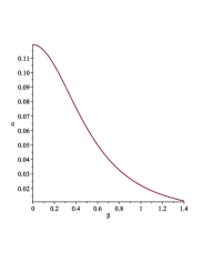
Figure 1: Dimensionless energy density ($\varrho=\frac{\rho\left(r\right)}{b_{0}}$) versus dimensionless parameter ($\beta=\sqrt{b_{0}}r$) with modified TMW mass function.

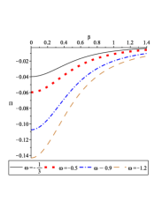
Figure 2: Dimensionless radial pressure ($\Pi=\frac{p_{r}\left(r\right)}{b_{0}}$) versus dimensionless parameter ($\beta=\sqrt{b_{0}}r$) with modified TMW mass function for different values of $\omega$.

To maintain the gravitational stability of DES, $g\left(r\right)$ should be negative. The gravity profile behavior is plotted versus $\omega$ and $\beta$ in both dark energy and phantom energy regimes for different values of $h_{\varepsilon}$ in Fig. 3. The range of $\beta$ is numerically determined according to the standard $g\left(r\right)$ range and $\omega$ values. Gravity profile values in the vicinity $\omega=-1/3$ are positive. As $h_{\varepsilon}$ increases, the range of $g\left(r\right)$ becomes more constrained and its positive values decrease. By reducing or removing the positive values of gravity profile, the model gets closer to the standard model of the dark energy star. Note that $h_{\varepsilon}=1$, refers to the gravity profile in general relativity Lobo2006 .

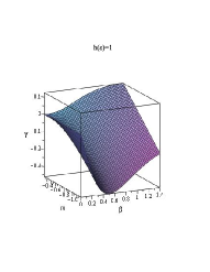
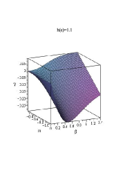
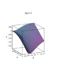
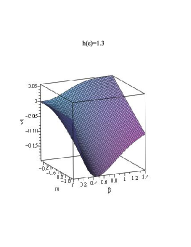
Figure 3: Three-dimensional diagram of the dimensionless gravity profile ($\gamma=\frac{g(r)}{b_{0}}$) versus dimensionless parameter ($\beta=\sqrt{b_{0}}r$) with modified TMW mass function for different values of $h_{\varepsilon}$. $h_{\varepsilon}=1$ (up left panel), $h_{\varepsilon}=1.1$ (up right panel), $h_{\varepsilon}=1.2$ (down left panel), and $h_{\varepsilon}=1.3$ (down right panel).

The anisotropy factor is shown in Figs. 4 and 5. It is observed that the anisotropy factor is positive for all $\omega$ values. There is also a slight difference between the anisotropy factor scheme with $h_{\varepsilon}=1$ (general relativity) and $h_{\varepsilon}=1.1$,$~{}1.2$, and $1.3$ (gravity’s rainbow).

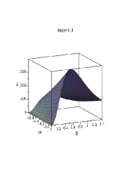
Figure 4: Three-dimensional diagram of the dimensionless anisotropy factor ($\delta=\frac{\Delta}{b_{0}}$) versus dimensionless parameter ($\beta=\sqrt{b_{0}}r$) with modified TMW mass function for different values of $h_{\varepsilon}$. $h_{\varepsilon}=1$ (up left panel), $h_{\varepsilon}=1.1$ (up right panel), $h_{\varepsilon}=1.2$ (down left panel), and $h_{\varepsilon}=1.3$ (down right panel).

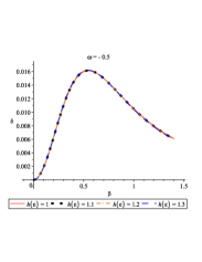
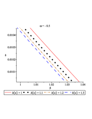
Figure 5: Dimensionless anisotropy factor ($\delta=\frac{\Delta(r)}{b_{0}}$) versus dimensionless parameter ($\beta=\sqrt{b_{0}}r$) with modified TMW mass function for different values of $h_{\varepsilon}$.

III Junction Condition and Dynamic Stability of Thin Shell

III.1 General Relativity

According to Darmois-Israel formalism in general relativity Israel1966 , we visualize two manifolds $M_{+}$ and $M_{-}$ with metrics $g_{\mu\nu}^{\pm}\left(x_{\pm}^{\mu}\right)$. These are matched together by two hypersurfaces $\Sigma_{\pm}$ with induced metrics $g_{ij}^{\pm}\left(\xi\right)$, where $\xi$ is the intrinsic coordinate of hypersurfaces. Note $\mu,\nu=0,1,2,3$ refer the coordinates of the $4-$dimensional manifold, and $i,j=1,2,3$ refer the coordinates of the $3-$dimensional shell. The induced metric on the junction surface is defined by the following relation Israel1966

$$g_{ij}=\left[g_{\mu\nu}\frac{\partial x^{\mu}}{\partial\xi^{i}}\frac{\partial x^{\nu}}{\partial\xi^{j}}\right]_{\pm}.$$ (22)

We select the parametric equation for a timelike hypersurface $\Sigma$ in the form $f\left(r,\tau\right)=r-a\left(\tau\right)=0$. The junction radius $a\left(\tau\right)$ is a function of proper time $\tau$. It is notable that $ds^{2}$ must be continuous throughout the junction. Using Eq. (22), the intrinsic metric to $\Sigma$ is written by Lobo2004

$$ds_{\Sigma}^{2}=-d\tau^{2}+a^{2}\left(\tau\right)\left(d\theta^{2}+\sin^{2}\theta d\varphi^{2}\right).$$ (23)

According to the parametric equation, it can be shown that the unit normal to the junction surfaceare $n_{\mu}$ defined as follows Poisson2004

$$n_{\mu}=\pm\frac{\frac{\partial f}{\partial x^{\mu}}}{\sqrt{g^{\alpha\beta}\frac{\partial f}{\partial x^{\alpha}}\frac{\partial f}{\partial x^{\beta}}}},$$ (24)

where $n^{\mu}n_{\mu}=+1$, and $u^{\mu}n_{\mu}=0$. Let us use the extrinsic curvature tensor $\kappa_{ij}$ of junction surface LoboC2005

$$\kappa_{ij}=-n_{\mu}\left(\frac{\partial^{2}x^{\mu}}{\partial\xi^{i}\partial\xi^{j}}+\Gamma_{\alpha\beta}^{\mu\pm}\frac{\partial x^{\alpha}}{\partial\xi^{i}}\frac{\partial x^{\beta}}{\partial\xi^{j}}\right).$$ (25)

The cause of the discontinuity in the extrinsic curvature is the presence of matter in the shell Mansouri1996 , thus the discontinuity in the extrinsic curvature is defined as Lobo2004

$$\chi_{ij}=\kappa_{ij}^{+}-\kappa_{ij}^{-},$$ (26)

and we can define the surface stress-energy tensor on $\Sigma$ Visser1989 ; Poisson1995

$$s_{\ j}^{i}=\frac{-1}{8\pi}\left(\chi_{~{}j}^{i}-\delta_{~{}j}^{i}\chi_{~{}k}^{k}\right).$$ (27)

This relation is known as the Lanczos equation, which roughly shows the dynamic behavior of the thin shell. We can obtain the non-zero components of the extrinsic curvature tensor $\kappa_{ij}$ LoboC2005 , by using Eqs. (24) and (25)

$$\kappa_{\theta}^{\theta\pm} = \frac{\sqrt{e^{-2\lambda_{\pm}\left(r\right)}+\overset{.}{a}^{2}}}{a},$$ (28)

$$\kappa_{\tau}^{\tau\pm} = \frac{\phi_{\pm}^{{}^{\prime}}\left(e^{-2\lambda_{\pm}\left(r\right)}+\overset{.}{a}^{2}\right)+\ddot{a}+\overset{.}{a}^{2}\lambda_{\pm}^{{}^{\prime}}}{\sqrt{e^{-2\lambda_{\pm}\left(r\right)}+\overset{.}{a}^{2}}}.$$ (29)

Here, we consider $s_{\ j}^{i}=diag\left(-\sigma,P,P\right)$ where $\sigma$ is the surface energy density and $P$ is tangential surface pressure. Also, the prime denotes a derivative with respect to junction radius ”$a$” and the overdot denotes a derivative with respect to the proper time, $\tau$. By using the Lanczos equation and Eqs. (28) and (29), the surface energy density and the surface pressure can be written as follow

$$\sigma = -\frac{\chi_{\theta}^{\theta}}{4\pi}=\frac{\sqrt{e^{-2\lambda_{-}\left(r\right)}+\overset{.}{a}^{2}}-\sqrt{e^{-2\lambda_{+}\left(r\right)}+\overset{.}{a}^{2}}}{4\pi a},$$ (30)

$$P = \frac{\chi_{\tau}^{\tau}+\chi_{\theta}^{\theta}}{8\pi}$$ (31)

$$= \frac{\left[\frac{\left(1+\phi^{{}^{\prime}}a\right)\left(e^{-2\lambda\left(r\right)}+\overset{.}{a}^{2}\right)+a\ddot{a}+\lambda^{{}^{\prime}}a\overset{.}{a}^{2}}{\sqrt{e^{-2\lambda\left(r\right)}+\overset{.}{a}^{2}}}\right]^{\pm}}{8\pi a},$$

where contractually, $\left[X\right]^{\pm}=X^{+}\left|\Sigma\right.-X^{-}\left|\Sigma\right.$ is displayed. Poisson and Visser Poisson1995 defined the $\eta=\frac{\sigma^{{}^{\prime}}}{P^{{}^{\prime}}}$ parameter, that $\sqrt{\eta}$ is the speed of sound. In the surface layer, it should be in range $0<\eta\leq 1$. By determining $\eta$, the stability regions can be identified.

III.2 Gravity’s Rainbow

To study thin shell and junction conditions in gravity’s rainbow, we can define the intrinsic metric to $\Sigma$ in gravity’s rainbow Eq. (22) and it given by Amirabi2018

$$ds_{\Sigma(\text{rainbow})}^{2}=-d\tau^{2}+\frac{a^{2}\left(\tau\right)}{h_{\varepsilon}^{2}}\left(d\theta^{2}+\sin^{2}\theta d\varphi^{2}\right),$$ (32)

where $\left(\tau,\theta,\varphi\right)$ refer the intrinsic coordinates. The line element should be continuous across $\Sigma$, therefore $\overset{.}{t}=\frac{\partial t}{\partial\tau}$ is given by

$$\overset{.}{t}_{(\text{rainbow})}=l_{\varepsilon}e^{\left(\lambda-\phi\right)_{\pm}}\sqrt{e^{-2\lambda_{\pm}\left(r\right)}+\frac{\overset{.}{a}^{2}}{h_{\varepsilon}^{2}}}.$$ (33)

The position of thin shell is given by $x^{\mu}=\left(t\left(\tau\right),a\left(\tau\right),\theta,\varphi\right)$, thus the $4-$velocity can be written as

$$u_{\pm(\text{rainbow})}^{\mu}=\left(l_{\varepsilon}e^{\left(\lambda-\phi\right)_{\pm}}\sqrt{e^{-2\lambda_{\pm}\left(r\right)}+\frac{\overset{.}{a}^{2}}{h_{\varepsilon}^{2}}},\overset{.}{a},0,0\right).$$ (34)

By using Eqs. (1) and (24), we obtain

$$n_{\pm(\text{rainbow})}^{\mu}=\left(\frac{l_{\varepsilon}\overset{.}{a}e^{\left(\lambda-\phi\right)_{\pm}}}{h_{\varepsilon}},\sqrt{h_{\varepsilon}^{2}e^{-2\lambda_{\pm}\left(r\right)}+\overset{.}{a}^{2}},0,0\right).$$ (35)

General form of $G_{\mu\nu}\left(\varepsilon\right)$ in gravity’s rainbow is same to general relativity, hence for a hypersurface, we can use the Lanczos equation in the same form of the Eq. (27). By using Eqs. (1), (28) and (29), the extrinsic curvature tensor $\kappa_{ij\left(\text{rainbow}\right)}$ is introduced in gravity’s rainbow by

$$\kappa_{\theta\left(\text{rainbow}\right)}^{\theta\pm} = \frac{\sqrt{h_{\varepsilon}^{2}e^{-2\lambda_{\pm}\left(r\right)}+\overset{.}{a}^{2}}}{a},$$ (36)

$$\kappa_{\tau\left(\text{rainbow}\right)}^{\tau\pm} = \frac{\phi_{\pm}^{{}^{\prime}}\left(h_{\varepsilon}^{2}e^{-2\lambda_{\pm}\left(r\right)}+\overset{.}{a}^{2}\right)+\ddot{a}+\overset{.}{a}^{2}\lambda_{\pm}^{{}^{\prime}}}{\sqrt{h_{\varepsilon}^{2}e^{-2\lambda_{\pm}\left(r\right)}+\overset{.}{a}^{2}}},$$ (37)

and also

$$\sigma_{\left(\text{rainbow}\right)} = -\frac{\chi_{\theta}^{\theta}}{4\pi}$$ (38)

$$= \frac{h_{\varepsilon}\left(\sqrt{e^{-2\lambda_{-}\left(r\right)}+\frac{\overset{.}{a}^{2}}{h_{\varepsilon}^{2}}}-\sqrt{e^{-2\lambda_{+}\left(r\right)}+\frac{\overset{.}{a}^{2}}{h_{\varepsilon}^{2}}}\right)}{4\pi a},$$

$$P_{\left(\text{rainbow}\right)} = \frac{\chi_{\tau}^{\tau}+\chi_{\theta}^{\theta}}{8\pi}=$$ (39)

$$= \frac{\left[\frac{\left(1+\phi^{{}^{\prime}}a\right)\left(h_{\varepsilon}^{2}e^{-2\lambda\left(r\right)}+\overset{.}{a}^{2}\right)+a\ddot{a}+\lambda^{{}^{\prime}}a\overset{.}{a}^{2}}{\sqrt{h_{\varepsilon}^{2}e^{-2\lambda\left(r\right)}+\overset{.}{a}^{2}}}\right]^{\pm}}{8\pi a}.$$

The interior spacetime in the presence of dark energy should match the exterior vacuum spacetime at a junction with $a$ radius. According to Eq. (1), we can write

$$e^{2\phi_{+}} = e^{-2\lambda_{+}}=1-\frac{2M}{r},$$ (40)

$$e^{-2\lambda_{-}} = 1-\frac{2m\left(r\right)}{h_{\varepsilon}^{2}r}=1-\frac{2M_{eff}}{r},$$ (41)

where $M_{eff}$ is the effective mass and it equals to $\frac{m\left(r\right)}{h_{\varepsilon}^{2}}$ (i.e., $M_{eff}=\frac{m\left(r\right)}{h_{\varepsilon}^{2}}$). Thus, the exterior spacetime is followed

$$ds_{+}^{2}=-\frac{1-\frac{2M}{r}}{l_{\varepsilon}^{2}}dt^{2}+\frac{dr^{2}}{h_{\varepsilon}^{2}\left(1-\frac{2M}{r}\right)}+\frac{r_{+}^{2}\left(d\theta^{2}+\sin^{2}\theta d\varphi^{2}\right)}{h_{\varepsilon}^{2}},$$ (42)

where $M$ is total mass. In order to avoid the event horizon in the dark energy star model, the junction radius places outside $a>2M$.

The surface energy density and the surface pressure, Eqs. (38) and (39), can be obtained in term of $m(r)$, $M$ and $h_{\varepsilon}$ as follows

$$\sigma_{\left(\text{rainbow}\right)} = \frac{h_{\varepsilon}\left(\sqrt{1-\frac{2m\left(a\right)}{ah_{\varepsilon}^{2}}+\frac{\overset{.}{a}^{2}}{h_{\varepsilon}^{2}}}-\sqrt{1-\frac{2M}{a}+\frac{\overset{.}{a}^{2}}{h_{\varepsilon}^{2}}}\right)}{4\pi a},$$ (43)

$$P_{\left(\text{rainbow}\right)} = \frac{1}{8\pi a}\left[\frac{h_{\varepsilon}^{2}\left(1-\frac{M}{a}\right)+\overset{.}{a}^{2}+\ddot{a}}{\sqrt{h_{\varepsilon}^{2}\left(1-\frac{2M}{a}\right)+\overset{.}{a}^{2}}}-\mathcal{P}\right],$$ (44)

where $\mathcal{P}=\frac{\left(1+\phi_{-}^{{}^{\prime}}a\right)\left(h_{\varepsilon}^{2}\left(1-\frac{2m\left(a\right)}{ah_{\varepsilon}^{2}}\right)+\overset{.}{a}^{2}\right)+a\ddot{a}+\frac{\left(am^{{}^{\prime}}\left(a\right)-m\left(a\right)\right)\overset{.}{a}^{2}}{h_{\varepsilon}^{2}\left(a-\frac{2m\left(a\right)}{h_{\varepsilon}^{2}}\right)}}{\sqrt{h_{\varepsilon}^{2}\left(1-\frac{2m\left(a\right)}{ah_{\varepsilon}^{2}}\right)+\overset{.}{a}^{2}}}$. From the above equations, it can be seen that $\sigma$ and $P$ depend on the rainbow function $h_{\varepsilon}$ and are independent of $l_{\varepsilon}$. According to the equation (6), we can define the area of junction sureface as $A_{\Sigma}=\frac{4\pi a^{2}}{h_{\varepsilon}^{2}}$, therefore the mass of a thin shell $m_{s}=\sigma_{\left(\text{rainbow}\right)}A_{\Sigma}$ in gravity’s rainbow is as follows

$$m_{s}=\frac{4\pi\sigma_{\left(\text{rainbow}\right)}a^{2}}{h_{\varepsilon}^{2}}.$$ (45)

By rewriting the Eq. (43) in terms of $M$, we can obtain the total mass at a static radius $a_{0}$

$$M = M_{eff}\left(a_{0}\right)$$ (46)

$$+m_{s}\left(a_{0}\right)h_{\varepsilon}\left(\sqrt{1-\frac{2M_{eff}\left(a_{0}\right)}{a_{0}}}-\frac{m_{s}\left(a_{0}\right)h_{\varepsilon}}{2a_{0}}\right).$$

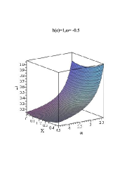
Figure 6: Three-dimensional diagrams of the stability regions. $X=\frac{m}{M}$ and $\alpha=\frac{a}{M}$, are the dimensionless.

As mentioned earlier, thin shell dynamical stability can be demonstrated using parameter $\eta$. Fig. 6 shows the stability region for the case $\omega=-0.5$ and different values of $h_{\varepsilon}$. It should be noted that we can use $b_{0}=2m\left[a^{3}\left(1-4m/a\right)\right]^{-1}$ as an auxiliary tool Lobo2006 , thus $a>4m\left(a\right)$. On the other hand, we assumed $a\gtrsim 2M$, so $0<\frac{m}{M}\lesssim\frac{1}{2}$. Note in these considerations, $h_{\varepsilon}$ is simplified. For $h_{\varepsilon}=1$, all equations yield to the usual form in general relativity. It can be inferred from Fig. 7 that as the value of the rainbow function $h_{\varepsilon}$ increases, the unstable regions near the Schwarzschild radius move closer to stability. For values $h_{\varepsilon}\geq 1.3$, the whole region is stable.

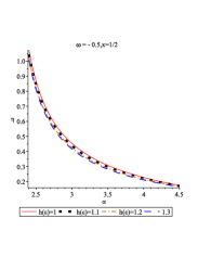
Figure 7: The stability region for DES versus $\alpha=\frac{a}{M}$.

IV ENERGY CONDITION

For interior region, the energy conditions are given by Leon1993 ; Visser1995
i) null energy condition (NEC): $\rho+p_{r}\geq 0$, and $\rho+p_{t}\geq 0$.
ii) weak energy condition (WEC): $\rho\geq 0$, $\rho+p_{r}\geq 0$, and $\rho+p_{t}\geq 0$.
iii) strong energy condition (SEC): $\rho+p_{r}+2p_{t}\geq 0$, and $\rho+p_{t}\geq 0$.
iv) dominant energy condition (DEC): $\rho\geq\left|p_{r}\right|$, and $\rho\geq\left|p_{t}\right|$.
By placing Eqs. (18), (19), and (21) in above definition for energy conditions, the interior energy conditions are obtained

$$\rho\left(r\right)+p_{r}\left(r\right) = \frac{b_{0}\left(2b_{0}r^{2}+3\right)\left(\omega+1\right)}{8\pi\left(2b_{0}r^{2}+1\right)},$$

$$\rho\left(r\right)-p_{r}\left(r\right) = \frac{-b_{0}\left(2b_{0}r^{2}+3\right)\left(\omega-1\right)}{8\pi\left(2b_{0}r^{2}+1\right)},$$

$$\rho\left(r\right)+p_{t}\left(r\right) = \frac{\frac{b_{0}}{8\pi}\left[\frac{8\mathcal{A}_{5}\left(b_{0}r^{2}+\frac{1}{2}\right)h_{\varepsilon}^{2}}{b_{0}r^{2}}+\mathcal{A}_{6}\right]}{\left(2b_{0}r^{2}+1\right)^{3}\left[\frac{\left(2b_{0}r^{2}+1\right)h_{\varepsilon}^{2}}{b_{0}r^{2}}-1\right]},$$

$$\rho\left(r\right)-p_{t}\left(r\right) = \frac{\frac{b_{0}}{8\pi}\left[\frac{8\mathcal{A}_{7}\left(b_{0}r^{2}+\frac{1}{2}\right)h_{\varepsilon}^{2}}{b_{0}r^{2}}-\mathcal{A}_{8}\right]}{\left(2b_{0}r^{2}+1\right)^{3}\left[\frac{\left(2b_{0}r^{2}+1\right)h_{\varepsilon}^{2}}{b_{0}r^{2}}-1\right]},$$

$$\rho\left(r\right)+p_{r}\left(r\right)+2p_{t}\left(r\right) = \frac{\frac{b_{0}}{4\pi}\left[\frac{4\mathcal{A}_{9}\left(b_{0}r^{2}+\frac{1}{2}\right)h_{\varepsilon}^{2}}{b_{0}r^{2}}+\mathcal{A}_{10}\right]}{\left(2b_{0}r^{2}+1\right)^{3}\left[\frac{\left(2b_{0}r^{2}+1\right)h_{\varepsilon}^{2}}{b_{0}r^{2}}-1\right]},$$ (47)

where $\mathcal{A}_{5}$, $\mathcal{A}_{6}$, $\mathcal{A}_{7}$, $\mathcal{A}_{8}$, $\mathcal{A}_{9}$ and $\mathcal{A}_{10}$ are

$$\mathcal{A}_{5} = b_{0}^{2}r^{4}-\frac{b_{0}r^{2}\left(\omega-4\right)}{2}+\frac{3}{4}\left(\omega+1\right),$$

$$\mathcal{A}_{6} = b_{0}^{2}r^{4}\left(\omega-1\right)\left(\omega+3\right)$$

$$+3b_{0}r^{2}\left(\omega-\frac{2}{3}\right)\left(\omega+3\right)+\frac{9\left(\omega^{2}-1\right)}{4},$$

$$\mathcal{A}_{7} = b_{0}^{2}r^{4}+\frac{b_{0}r^{2}\left(\omega+4\right)}{2}-\frac{3}{4}\left(\omega-1\right),$$

$$\mathcal{A}_{8} = b_{0}^{2}r^{4}\left(\omega^{2}+2\omega-5\right)$$

$$+3b_{0}r^{2}\left(\omega^{2}+\frac{7\omega}{3}+\frac{10}{3}\right)+\frac{3\left(3\omega^{2}+5\right)}{4},$$

$$\mathcal{A}_{9} = b_{0}^{2}r^{4}\left(\omega+1\right)+b_{0}r^{2}\left(\omega+2\right)+\frac{3\left(3\omega+1\right)}{4},$$

$$\mathcal{A}_{10} = b_{0}^{2}r^{4}\left(\omega^{2}-1\right)$$

$$+3b_{0}r^{2}\left(\omega^{2}+\omega-\frac{2}{3}\right)+\frac{3\left(3\omega^{2}-2\omega-1\right)}{4}.$$

The energy conditions are demonstrated in Fig. 8 for cases $h_{\varepsilon}=1$, and $h_{\varepsilon}=1.3$, respectively.

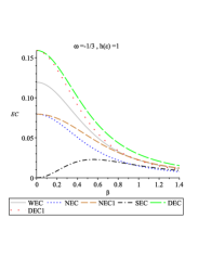
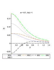
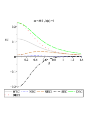
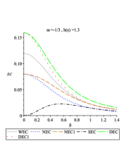
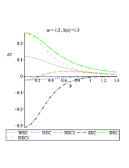
Figure 8: The energy conditions per $b_{0}$ in the interior of DES versus $\beta=\sqrt{b_{0}}r$. Note NEC1 and DEC1 refer to ($\rho+p_{t}\geq 0$) and ($\rho\geq\left|p_{t}\right|$), respectively.

It can be seen in gravity’s rainbow similar to general relativity, for $\omega=-\frac{1}{3}$, all energy conditions are obeyed by our calculations. For $-\frac{1}{3}\leq\omega\leq-1$, all conditions are satisfied except SEC. Violation of strong energy condition is a feature of dark energy. For $\omega<-1$, SEC and NES conditions are violated. Violation of null energy condition is a feature of phantom energy.

V Conclusions

In this study, by assuming the existence of an anisotropic distribution of dark energy in the interior of spherically symmetric spacetime, we got a modified TOV equation of anisotropic distribution in the gravity’s rainbow. In order to solve the energy-dependent field equations, we used the modified Tolman-Matese-Whitman mass function. We considered the dark energy equations of state to obtain the properties of dark energy stars. We showed that the final solution is independent of the rainbow function $l_{\varepsilon}$, and it only depends on $h_{\varepsilon}$. As the value of $h_{\varepsilon}$ increased, the gravity profile$\ g\left(r\right)$ became more constrained thus the model is closer to the standard definition of a dark energy star, and the anisotropy factor remain positive. As the rainbow function equals one, this solution tends to the general relativity Lobo2006 . We also investigated the dynamical stability of thin shell for the dark energy star in this gravity by generalizing the Darmois-Israel formalism in the gravity’s rainbow. We showed that by increasing rainbow function $h_{\varepsilon}$, the unstable regions near the event horizon decrease. The strong energy condition (SEC) is violated in the interior of the dark energy star. It seems that employing the gravity’s rainbow has the greatest effect near where the phase transition zone is called. Where it is located near the event horizon and high-energy particles decay there due to crossing the critical surface Chapline ; ChaplinearXiv . The presence of modified gravity with quantum gravity backgrounds will significantly help to study the behavior of a dark energy star, especially near the critical region.

References

• (1) G. Chapline, Int. J. Mod. Phys. A 18 (2003) 3587.
• (2) P. O. Mazur, and E. Mottola, Proc. Nat. Acad. Sci. 101 (2004) 9545.
• (3) M. Visser, and D. L. Wiltshire, Class. Quantum Grav. 21 (2004) 1135.
• (4) C. Cattoen, T. Faber, and M. Visser, Class. Quantum Grav. 22 (2005) 4189.
• (5) G. Chapline, ”Dark Energy Stars”, [arXiv:astro-ph/0503200].
• (6) T. Koivisto, and D. F. Mota, Astrophys. J. 679 (2008) 1.
• (7) T. Koivisto, and D. F. Mota, JCAP 06 (2008) 018.
• (8) L. Campanelli, et al., Int. J. Mod. Phys. D 20 (2011) 1153.
• (9) A. I. Sokolov, J. Exp. Theor. Phys. 52 (1980) 575.
• (10) J. B. Hartle, R. F. Sawyer, and D. J. Scalapino, Astrophys. J. 199 (1975) 471.
• (11) G. H. Bordbar, and M. Karami, Eur. Phys. J. C 82 (2022) 1.
• (12) V. V. Usov, Phys. Rev. D 70 (2004) 067301.
• (13) F. S. Lobo, and P. Crawford, Class. Quantum Grav. 22 (2005) 4869.
• (14) F. S. Lobo, Class. Quantum Grav. 23 (2006) 1525.
• (15) C. R. Ghezzii, Astrophys. Space Sci. 333 (2011) 437.
• (16) S. S. Yazadjiev, Phys. Rev. D 83 (2011) 127501.
• (17) P. Bhar, and F. Rahaman, Eur. Phys. J. C 75 (2015) 1.
• (18) P. Bhar, et al., Can. J. Phys. 96 (2018) 594.
• (19) P. Beltracchi, and P. Gondolo, Phys. Rev. D 99 (2019) 044037.
• (20) A. Banerjee, M. Jasim, and A. Pradhan, Mod. Phys. Lett. A 35 (2020) 2050071.
• (21) G. Panotopoulos, A. Rincón, and I. Lopes, Phys. Dark Universe. 34 (2021) 100885.
• (22) M. F. A. Rangga Sakti, and A. Sulaksono, Phys. Rev. D 103 (2021) 084042.
• (23) M. Malaver, et al., ”A theoretical model of Dark Energy Stars in Einstein-Gauss-Bonnet Gravity”, [arXiv:2106.09520].
• (24) P. Bhar, Phys. Dark Universe. 34 (2021) 100879.
• (25) J. Magueijo, and L. Smolin, Class. Quantum Grav. 21 (2004) 1725.
• (26) P. Galan, and G. A. Mena Marugan, Phys. Rev. D 70 (2004) 124003.
• (27) J. Hackett, Class. Quantum Grav. 23 (2006) 3833.
• (28) R. Aloisio, et al., Phys. Rev. D 73 (2006) 045020.
• (29) Y. Ling, X. Li, and H. Zhang, Mod. Phys. Lett. A 22 (2007) 2749.
• (30) R. Garattini, and B. Majumder, Nucl. Phys. B 884 (2014) 125.
• (31) Z. Chang, and S. Wang, Eur. Phys. J. C 75 (2015) 259.
• (32) G. Santos, G. Gubitosi, and G. Amelino-Camelia, JCAP 08 (2015) 005.
• (33) A. F. Ali, et al., Int. J. Geom. Meth. Mod. Phys. 12 (2015) 1550085.
• (34) P. Galan, and G. A. Mena Marugan, Phys. Rev. D 74 (2006) 044035.
• (35) Y. Ling, X. Li, and H. Zhang, Mod. Phys. Lett. A 22 (2007) 2749.
• (36) A. F. Ali, M. Faizal, and M. M. Khalil, JHEP 12 (2014) 159.
• (37) S. H. Hendi, et al., Eur. Phys. J. C 76 (2016) 150.
• (38) Y. -W. Kim, S. K. Kim, and Y. -J. Park, Eur. Phys. J. C 76 (2016) 557.
• (39) S. H. Hendi, et al., Eur. Phys. J. C 76 (2016) 296.
• (40) S. Gangopadhyay, and A. Dutta, Europhys. Lett. 115 (2016) 50005.
• (41) S. H. Hendi, et al., Eur. Phys. J. C 77 (2017) 647.
• (42) S. Alsaleh, Int. J. Mod. Phys. A 32 (2017) 1750076.
• (43) Z. -W. Feng, and S. -Z. Yang, Phys. Lett. B 772 (2017) 737.
• (44) B. Eslam Panah, Phys. Lett. B 787 (2018) 45.
• (45) S. Upadhyay, et al., Prog. Theor. Exp. Phys. 2018 (2018) 093E01
• (46) B. Eslam Panah, S. Panahiyan, and S. H. Hendi, Prog. Theor. Exp. Phys. 2019 (2019) 013E02.
• (47) P. H. Morais, et al., Gen. Relativ. Gravit. 54 (2022) 16.
• (48) B. Hamil, and B. C. Lütfüoğlu, Int. J. Geom. Meth. Mod. Phys. 19 (2022) 2250047.
• (49) S. H. Hendi, et al., JCAP 09 (2016) 013.
• (50) R. Garattini, and G. Mandanici, Eur. Phys. J. C 77 (2017) 57.
• (51) B. Eslam Panah, et al., Astrophys. J. 848 (2017) 24.
• (52) U. Debnath, Eur. Phys. J. Plus 136 (2021) 442.
• (53) C. E. Mota, et al., Class. Quantum Grav. 39 (2022) 085008.
• (54) S. S. Bayin, Astrophys. J. 303 (1986) 101.
• (55) M. S. Morris, and K. S. Thorne, Am. J. Phys. 56 (1988) 395.
• (56) W. Israel, ”Singular hypersurfaces and thin shells in general relativity”. Il Nuovo Cimento B. 44 (1966) 1.
• (57) F. S. Lobo, Class. Quantum Grav. 21 (2004) 4811.
• (58) E. Poisson, ”A relativist’s toolkit: the mathematics of black-hole mechanics”. Cambridge university press (2004).
• (59) R. Mansouri, and M. Khorrami, J. Math. Phys. 37 (1996) 5672.
• (60) M. Visser, Nucl. Phys. B 328 (1989) 203.
• (61) E. Poisson, and M. Visser, Phys. Rev. D 52 (1995) 7318.
• (62) Z. Amirabi, M. Halilsoy, and S. H. Mazharimousavi, Mod. Phys. Lett. A 33 (2018) 1850049.
• (63) J. P. de Leon, Gen. Relativ. Gravit. 25 (1993) 1123.
• (64) M. Visser, ”Lorentzian Wormholes. From Einstein to Hawking”. Woodbury, 1995.