Tideless Traversable Wormholes surrounded by cloud of strings in f(R) gravity

Abstract

We study the tideless traversable wormholes in the $f(R)$ gravity metric formalism. First we consider three shape functions of wormholes and study their viabilities and structures. The connection between the $f(R)$ gravity model and wormhole shape function has been studied and the dependency of the $f(R)$ gravity model with the shape function is shown. We also obtain a wormhole solution in the $f(R)$ gravity Starobinsky model surrounded by a cloud of strings. In this case, the wormhole shape function depends on both the Starobinsky model parameter and the cloud of strings parameter. The structure and height of the wormhole is highly affected by the cloud of strings parameter, while it is less sensitive to the Starobinsky model parameter. The energy conditions have been studied and we found the ranges of the null energy condition violation for all wormhole structures. The quasinormal modes from these wormhole structures for the scalar and Dirac perturbations are studied using higher order WKB approximation methods. The quasinormal modes for the toy shape functions depend highly on the model parameters. In case of the Starobinsky model’s wormhole the quasinormal frequencies and the damping rate increase with an increase in the Starobinsky model parameter in scalar perturbation. Whereas in Dirac perturbation, with an increase in the Starobinsky model parameter the quasinormal frequencies decrease and the damping rate increases. The cloud of strings parameter also impacts prominently and differently the quasinormal modes from the wormhole in the Starobinsky model.

I Introduction

Recent experimental observations suggest that the universe is undergoing a phase of accelerated expansion Riess_2001 ; Perlmutter_1999 ; Bennett_2003 . Since General Relativity (GR) can’t explain this current phase of expansion of the universe, several modifications to GR have been introduced including dark energy models and Modified Gravity Theories (MGTs) Sami . In MGTs, the curvature part of Lagrangian is modified to explain the observational results. One of the attractive and simplest forms of such extensions is the $f(R)$ theories of gravity, where the Ricci scalar $R$ in the Lagrangian or action of GR is replaced by an arbitrary function of $R$. Some of the promising $f(R)$ gravity models are: Starobinsky model Starobinsky1980 , Hu-Sawicki model hu_sawicki , Tsujikawa model Tsujikawa , Gogoi-Goswami model gogoi2 etc. Of late, there are many works in which the viabilities and different aspects of these models have been explicitly studied gogoicosmology ; jbora ; BHu ; Martinelli2009 ; Asaka2016 ; Cen2019 ; Baruah2021 ; Parbin2022 . Apart from these, various other $f(R)$ gravity models are studied in different perspectives Sotiriou2006 ; Huang2014 ; Lu2016 ; Nojiri2007 ; Cognola2008 ; Felice2010 ; Bamba2011 ; Bamba2010 ; Bamba2012 ; Sebastiani2014 ; Thakur2013 ; Bamba2014 ; Sebastiani2018 ; Motohashi2017 ; Astashenok2017 ; Bahamonde2017 ; Faraoni2017 ; Abbas2017 ; Sussman2017 ; Mongwane2017 ; Mansour2018 ; Papagiannopoulos2018 ; Oikonomou2018 ; Castellanos2018 ; Samanta2020 ; Kalita2021 ; Sarmah2022 ; Kalita2022 .

Like GR, MGTs also show the possibilities of black holes and wormholes. Recent studies show that the MGTs play a very important role in the study of black holes and wormholes. It is seen that the black hole solutions, black hole thermodynamics and quasinormal modes are affected by the type of modifications introduced in the extended forms of gravity gogoi3 ; Gogoi_bumblebee . Lately, it was found that the polarization modes of Gravitational Waves (GWs) increase from two to three in $f(R)$ theory metric formalism due to the existence of extra degrees of freedom. The extra polarization mode is a scalar massive polarization mode which is a mixture of the massless transverse but not traceless breathing scalar mode and the massive longitudinal scalar mode gogoi2 ; gogoi1 . In recent times there are plenty of works in literature that are related to the study of different aspects of wormholes in the $f(R)$ theory of gravity. For example, in Ref. Lobo2009 , the traversable wormholes have been studied in the framework of $f(R)$ gravity. In this work, the authors have explicitly studied the factors responsible for the null energy condition violation supporting the existence of wormholes for different shape functions. The cosmological model with a traversable wormhole has been studied in Ref. Kim1996 . In Ref. Bronnikov:2010tt , existence of wormholes in scalar tensor theory and $f(R)$ gravity has been studied. In another study, the cosmological evolution of wormhole solutions in $f(R)$ gravity has been explored Bahamonde2016 . This study deals with the construction of dynamical wormhole that asymptotically approaches a Friedmann-Lemaître-Robertson-Walker universe. Traversable wormholes in $f(R)$ gravity with non-commutative geometry has been studied in Ref. Kuhfittig2018 . In this work, the author has studied the relation of wormhole shape function with the $f(R)$ gravity model explicitly and also studied the associated energy conditions at the throat of the wormhole. Exactly traversable wormholes in bumblebee gravity have been obtained recently in Ref. Jusufi19 . The thin-shell wormholes in quadratic $f(R)$ gravity have been studied in Ref. Eiroa2016 , where the authors present a class of spherically symmetric Lorentzian wormholes in inflationary Starobinsky type model with and without charge. The authors constructed the wormholes by cutting and pasting two manifolds with different constant curvatures into a hypersurface representing the throat of the wormhole which is not symmetric across the throat. Wormholes in $f(R)$ gravity sourced by a phantom scalar field have been recently studied in Ref. Karakasis2022 , where the authors obtained exact wormhole solutions and studied the energy conditions explicitly by considering a scalar field with negative kinetic energy, a phantom scalar field which has a self interacting potential. In their study, they have obtained the wormhole solution without specifying the actual form of the $f(R)$ function. They show that the presence of such a scalar field has impacts on the scalar curvature and the size of the wormhole throat. An increase in the strength of the scalar field results in wormholes with larger throat radii, which eventually decreases the curvature near the wormhole. The traversable wormhole geometries using Karmarkar condition have been studied in Ref. Shamir2020 . In Ref. Chervon2021 , the authors have studied the wormholes and black holes in $f(R)$ gravity with a kinetic curvature scalar. Traversable wormholes in the $R+\alpha R^{n}$ model were studied by N. Godani and G. C. Samanta in Ref. Godani2020 . Deflection angle of the Brane-Dicke wormhole in the weak field limit has been studied in Ref. Javed2019 . In another work, the weak deflection angle by black holes and wormholes has been extensively studied with different examples and wormhole structures Ovgun202101 . Apart from these, there are several studies dealing with deflection angle in the domain of black holes and wormholes Javed2022 ; Ovgun2020d ; Pantig202202 ; Javed202201 ; Javed202202 . Traversable wormholes in extended teleparallel gravity with matter coupling is studied in Ref. Mustafa2021 , where the authors explored mainly non-commutative Lorentzian and Gaussian distributed wormholes explicitly. An evolving wormhole hole configuration is studied in the dark matter halo in Ref. Ovgun202102 .

It is worth to be mentioned that the wormhole solutions are primarily useful as “gedanken-experiments” and as a theoretical probe of the possible results of GR. In basic GR, wormholes are supported by exotic matters. These exotic matters involve a stress-energy tensor which can violate the Null Energy Condition (NEC) Morris:1988cz ; Visser . The NEC is defined by $T_{\mu\nu}k^{\mu}k^{\nu}\geq 0$, where $k^{\mu}$ is any null vector. Hence, in wormhole physics it is an important challenge to find any realistic matter source which can violate the NEC.

The quasinormal modes of black holes have been studied extensively in different MGTs gogoi3 ; qnm_bumblebee ; Bhatta2018 ; Liu2022 ; Ovgun201802 ; Okyay2022 ; Karmakar2022 ; Gonzal2010 ; Pantig202201 ; Yang2022 . In such a study, it was seen that the quasinormal modes from black holes may play a very important part in distinguishing GR from $f(R)$ gravity Bhatta2018 . Along with the black holes, the quasinormal modes of wormholes also have received significant attention from the researchers. The quasinormal modes of a natural anti-de Sitter wormhole in Einstein-Born-Infeld gravity have been extensively studied in Ref. Kim2018 . Authors in this paper studied the dependencies of the quasinormal modes from the wormholes on the mass of the scalar field as well as on other wormhole parameters. Recently, quasinormal modes from a wormhole in bumblebee gravity have been studied in Ref. Oliveira2019 . It has been shown recently that similar to black holes, the arbitrarily long lived modes or quasi-resonances can also exist in case of a wormhole if it does not have a constant red-shift function Churilova2020 . The quasinormal modes, echoes and shadows of wormholes without exotic matter were studied in Ref. Churilova2021 . Apart from these studies, there are many recent studies which involves different properties of wormholes as well as quasinormal modes and echoes Kim2008 ; Jusufi2021 ; Dutta2020 ; Gonz2022 ; Aneesh2018 ; Blaz2018 ; Bronnikov2021 ; Volkel2018 ; Bueno2018 ; Bronnikov2020 ; Ovgun2018 ; Jusufi2018 ; Halilsoy2014 ; Jusufi2017 ; Ovgun2016 ; Ovgun2016_2 ; Liu2021 ; Junior2020 . Being motivated from these studies, we study wormholes in the $f(R)$ gravity Starobinsky model and in the models defined by three shape functions in this work. At first, we use three different types of wormhole shape functions and study their viability conditions. After that we show the dependency of the shape functions with $f(R)$ gravity model in presence of cloud of strings. In the next stage, we consider the $f(R)$ gravity Starobinsky model and obtain the wormhole solution surrounded by a cloud of strings. The idea of cloud of strings in GR has been implemented for the first time in Ref. Letelier1979 . Since then the cloud of strings has been used by many researchers in different perspectives Ganguly2014 ; Bronnikov2016 ; Herscovich2010 ; Ghosh2014 ; Younesizadeh2022 ; Badawi2022 ; Belhaj2022 ; Sood2022 ; Ali2021 ; Singh2020 . The impact of the cloud of strings on wormholes in GR has been studied previously in Ref. Richarte2008 . However, in our work, we shall consider this relic in $f(R)$ gravity to obtain the wormhole solutions. Such a study will help us to see the impact of clouds of strings on the shape of the wormholes. Apart from this, we shall study the quasinormal modes of such wormholes using the WKB approximation method. A comparative study with the previously used wormhole shape functions will be done to get a clear view on the quasinormal mode dependencies on the shape functions. This study will also provide some important insights on the possibilities of wormholes and chances of detecting them using the quasinormal modes for the considered $f(R)$ gravity models. It will also provide the possibilities of differentiating a wormhole and a black hole in terms of quasinormal modes. In our work, we shall consider two types of perturbations. The general scalar perturbation and Dirac perturbation. The scalar field perturbation is commonly used in different studies to check the behaviour of the quasinormal modes and a study of scalar quasinormal modes in wormhole spacetime will help us to compare the results easily with quasinormal modes from black holes. On the other hand, interaction of the Dirac field with gravity has been studied in Ref.s Finster1999 ; Finster1999_2 . It was found that the time-periodic solutions in various black hole spacetimes do not exist Finster2000 ; Finster2000_2 . This implies that any Dirac particles, such as electrons, neutrinos etc. cannot remain on a periodic orbit around a black hole. So, if such particles around a black hole or wormhole collapses gravitationally, they should vanish inside the event horizon of a black hole or they can escape to infinity. Hence a study of the Dirac fields in curved background spacetimes can provide interesting results. In this study, we shall study such Dirac field perturbations on the wormhole spacetimes considered in the work.

We have already discussed that quasinormal modes from wormholes have been studied widely in different literatures. Although wormholes are still considered to be hypothetical, one can see that GR exhibits both black holes and wormholes as promising solutions of the field equation. Since GR has been one of the most successful theories of gravity till now in predicting physically realizable things, the possibility of existence of wormholes in the Universe can not be nullified. If that is so, tools and methods to probe wormholes and also differentiating them from black holes is an essential need for the scientific community. As previous studies show that wormholes also can emit quasinormal modes when a perturbation is introduced to its background, we believe that studies dealing with quasinormal modes from wormholes can play a significant role in differentiating black holes from wormholes in the near future when suitable observational data of quasinormal modes will be obtained.

The primary motivation of this work is to see how the structure of a wormhole behaves in presence of a cloud of strings in $f(R)$ gravity and possibility of experimental detection of the impacts of a cloud of strings in the wormhole background using quasinormal modes as a probe. The study will also focus on the variation of the quasinormal modes with the cloud of string parameter and the $f(R)$ gravity model parameters in order to understand how they can affect the ringdown GWs. The justification for using the $f(R)$ gravity Starobinsky model is its simplicity and versatility. Since the Starobinsky model has been very successful in explaining the inflationary epoch of the Universe and several other observational aspects, it has been the choice of many researchers to consider it in different directions of study. This investigation dealing with the Starobinsky model will put some light on the possible configuration of wormholes in this model as well as its behaviour and properties of quasinormal modes.

The rest of the structure of this paper is as follows. We have given a brief introduction of wormholes in $f(R)$ gravity in section II. Here we have studied the field equations and connection between shape function and $f(R)$ gravity model. We have obtained a wormhole solution in $f(R)$ gravity Starobinsky model in this section and then studied the energy conditions in brief for a general idea. In section III, we have studied quasinormal modes of the wormhole solution obtained in the Starobinsky model along with three other toy shape functions for the scalar perturbations and Dirac perturbations. The time domain analysis part has been included in section IV. We have summarized the results of our work with a brief conclusion in section V.

II Wormholes in $f(R)$ gravity

In this work, we shall use the metric formalism in which the action of the theory is varied with respect to the metric $g^{\mu\nu}$. The $f(R)$ gravity in metric formalism has been widely studied in the field of black holes and wormholes previously. Other formalisms frequently used in literature are the Palatini formalism Sotiriou2005 and the metric-affine formalism Sotiriou:2006qn . In the Palatini formalism, the metric and the connections are considered as independent or separate variables and the matter action is independent of the connection, while in the metric-affine formalism the matter part of the action is also varied with respect to the connection. In our work, we shall restrict to the study of wormholes in $f(R)$ gravity metric formalism only.

The action in $f(R)$ gravity is given by

$$S=\frac{1}{2\kappa}\int d^{4}x\sqrt{-g}\;f(R)+\int d^{4}x\sqrt{-g}\;{\cal L}_{m}(g_{\mu\nu},\psi)\,,$$ (1)

here $\kappa=8\pi G$ and from hereafter we shall consider $\kappa=1$. ${\cal L}_{m}$ is the matter Lagrangian density, in which matter is minimally coupled to the metric $g_{\mu\nu}$ and $\psi$ denotes the matter fields. Now varying the action (1) with respect to the metric $g^{\mu\nu}$, we obtain the field equations in $f(R)$ gravity metric formalism as given by

$$\mathcal{F}R_{\mu\nu}-\frac{1}{2}f\,g_{\mu\nu}-\nabla_{\mu}\nabla_{\nu}\mathcal{F}+g_{\mu\nu}\Box\mathcal{F}=\,T^{(m)}_{\mu\nu}\,,$$ (2)

where $\mathcal{F}\equiv df(R)/dR$ and $T^{(m)}_{\mu\nu}=-\frac{2}{\sqrt{-g}}\frac{\delta\left(\sqrt{-g}\,{\cal L}_{m}\right)}{\delta g^{\mu\nu}}$ is the stress-energy tensor of the matter. Taking trace of this Eq. (2), we have

$$\mathcal{F}R-2f+3\,\Box\mathcal{F}=\,T.$$ (3)

Using this trace equation we can rewrite the field Eq. (2) in the following possible form:

$$G_{\mu\nu}\equiv R_{\mu\nu}-\frac{1}{2}R\,g_{\mu\nu}=T^{{\rm eff}}_{\mu\nu}\,.$$ (4)

Here the effective stress-energy tensor is $T^{{\rm eff}}_{\mu\nu}=T^{(c)}_{\mu\nu}+\tilde{T}^{(m)}_{\mu\nu}$, where $\tilde{T}^{(m)}_{\mu\nu}=T^{(m)}_{\mu\nu}/\mathcal{F}$ and the curvature stress-energy tensor,

$$T^{(c)}_{\mu\nu}=\frac{1}{\mathcal{F}}\left[\nabla_{\mu}\nabla_{\nu}\mathcal{F}-\frac{1}{4}g_{\mu\nu}\left(R\mathcal{F}+\Box\mathcal{F}+T\right)\right].$$ (5)

The associated conservation law with the modified field equation can be given by

$$\nabla^{\mu}T^{(c)}_{\mu\nu}=\frac{1}{\mathcal{F}^{2}}T^{(m)}_{\mu\nu}\nabla^{\mu}\mathcal{F}.$$ (6)

As mentioned earlier, since the possibility that wormholes are supported by $f(R)$ theories of gravity, here our intention is to explore the distinguishing characteristics of a few specific forms of wormholes in this area of MGTs. One should note that it is the effective stress energy of $f(R)$ gravity, which may be interpreted as a gravitational fluid, is responsible for the null energy condition violation. This leads to the non-standard wormhole geometries, fundamentally different from their counterparts in GR Lobo2009 . However, we demand that the matter threading the wormhole satisfies the energy conditions. For the purpose of our study we consider the following ansatz,

$$ds^{2}=-e^{2\Phi(r)}dt^{2}+\frac{dr^{2}}{1-b(r)/r}+r^{2}\,(d\theta^{2}+\sin^{2}{\theta}\,d\phi^{2})\,,$$ (7)

where $\Phi(r)$ and $b(r)$ are arbitrary functions of the radial coordinate $r$, referred to as the lapse function and the shape function respectively Morris:1988cz . This ansatz represents a static and spherically symmetric wormhole in spacetime. The lapse function determines the red-shift effect and tidal force associated with the wormhole spacetime. If the lapse function $\Phi(r)=0$ or $e^{2\Phi(r)}=1$, the wormhole is said to be tideless Konoplya2018 .

It is to be noted here is that the radial coordinate $r$ is non-monotonic which decreases from infinity to minimum value $r=r_{0}$ at the throat of the wormhole, defined by $b(r_{0})=r_{0}$, and it then again increases to infinity. Hence, the shape function $b(r)$ has the minimum value $r_{0}$ at the throat of the wormhole. In general to have a wormhole solution certain conditions should be satisfied including the flaring out condition of the throat, given by $(b-b^{\prime}r)/b^{2}>0$ Morris:1988cz at the throat $b(r_{0})=r_{0}$ and the condition $b^{\prime}(r_{0})<1$. These conditions impose the NEC violation in the classical GR. Another condition for a stable wormhole is $1-b(r)/r>0$. Most importantly, for the wormhole to be traversable, there should be no horizons present, which are defined on the spacetime by $e^{2\Phi}\rightarrow 0$, so that $\Phi(r)$ must be finite everywhere. In view of this, we consider a constant redshift function i.e. $\Phi^{\prime}=0$. This simplifies the calculations associated with the field equations and provide interesting wormhole solutions.

The unusual structure of wormhole suggests that the distribution of matter threading the wormhole is anisotropic and the stress-energy tensor for such distribution of matter is given by

$$T^{(m)}_{\mu\nu}=(\rho+p_{t})U_{\mu}\,U_{\nu}+p_{t}\,g_{\mu\nu}+(p_{r}-p_{t})\chi_{\mu}\chi_{\nu}\,,$$ (8)

where $U^{\mu}$ represents the four-velocity of matter field, $\chi^{\mu}=\sqrt{1-b(r)/r}\,\delta^{\mu}{}_{r}$ represents the unit spacelike vector along the radial direction, $\rho(r)$ represents the energy density, $p_{r}(r)$ represents the radial pressure along the direction of $\chi^{\mu}$, and $p_{t}(r)$ represents the transverse pressure along the direction orthogonal to $\chi^{\mu}$. Using this stress-energy tensor of matter, we can write the field equations (4) in the following forms:

$$\frac{b^{\prime}}{r^{2}} =\frac{\rho}{\mathcal{F}}+\frac{\left(\mathcal{F}R+\Box\mathcal{F}+T\right)}{4\mathcal{F}}\,,$$ (9)

$$-\frac{b}{r^{3}} =\frac{p_{r}}{\mathcal{F}}+\frac{1}{\mathcal{F}}\Bigg{\{}\left(1-\frac{b}{r}\right)\left[\mathcal{F}^{\prime\prime}-\mathcal{F}^{\prime}\frac{b^{\prime}r-b}{2r^{2}(1-b/r)}\right]-\frac{1}{4}\left(\mathcal{F}R+\Box\mathcal{F}+T\right)\Bigg{\}}\,,$$ (10)

$$-\frac{b^{\prime}r-b}{2r^{3}} =\frac{p_{t}}{\mathcal{F}}+\frac{1}{\mathcal{F}}\left[\left(1-\frac{b}{r}\right)\frac{\mathcal{F}^{\prime}}{r}-\frac{1}{4}\left(\mathcal{F}R+\Box\mathcal{F}+T\right)\right],$$ (11)

where a prime denotes a derivative with respect to the radial coordinate $r$. In the above equations, $\Box\mathcal{F}$ is given by

$$\Box\mathcal{F}=\left(1-\frac{b}{r}\right)\left[\mathcal{F}^{\prime\prime}-\frac{b^{\prime}r-b}{2r^{2}(1-b/r)}\,\mathcal{F}^{\prime}+\frac{2\mathcal{F}^{\prime}}{r}\right]$$ (12)

and the Ricci curvature scalar $R$ is given by

$$R = \frac{2b^{\prime}}{r^{2}}\,.$$ (13)

Rearranging the field equations (9), (10) and (11) we may obtain the following expressions for $\rho$, $p_{r}$ and $p_{t}$ Lobo2009 as

$$\rho =\frac{\mathcal{F}b^{\prime}}{r^{2}}\,,$$ (14)

$$p_{r} =-\frac{b\mathcal{F}}{r^{3}}+\frac{\mathcal{F}^{\prime}}{2r^{2}}(b^{\prime}r-b)-\mathcal{F}^{\prime\prime}\left(1-\frac{b}{r}\right),$$ (15)

$$p_{t} =-\frac{\mathcal{F}^{\prime}}{r}\left(1-\frac{b}{r}\right)+\frac{\mathcal{F}}{2r^{3}}(b-b^{\prime}r).$$ (16)

These are the generic forms of expressions of the energy density and pressures of the matter threading the wormhole in $f(R)$ gravity metric formalism as a function of the wormhole shape function and $\mathcal{F}(r)$.

II.1 Toy Models of Wormhole Shape Function

As the shape function of a wormhole is the deciding factor for its particular construction or structure, it is necessary to study the behaviours of this function of a wormhole under certain required conditions. It is to be noted that in order to have a consistent wormhole structure the shape function should satisfy the following conditions or properties: $(i)\;b(r)/r<1$ for $r>r_{0},$ $(ii)\;b(r)=r_{0}$ at $r=r_{0},$ $(iii)\;b(r)/r\rightarrow 0$ as $r\rightarrow\infty,$ $(iv)\;b(r)-b^{\prime}(r)r>0$ and $(v)\;b^{\prime}(r)<1$ at $r=r_{0}.$ In this study, we consider three toy wormhole shape functions as given by

$$b_{1}(r)=r\exp\left[{m_{1}\left(r_{0}-r\right)}\right],$$ (17)

$$b_{2}(r)=\frac{r\log\left(2m_{2}\ r_{0}\right)}{\log\left[m_{2}\left(r+r_{0}\right)\right]},$$ (18)

and

$$b_{3}(r)=\frac{m_{3}\ r}{m_{3}+r-r_{0}}.$$ (19)

Here $m_{1},m_{2}$ and $m_{3}$ are the model parameters and $r_{0}$ denotes the throat radius of the wormholes. The first toy model has been widely used in different works exp_shape01 ; exp_shape02 ; exp_shape03 . Whereas other two toy functions have been introduced by us as two possible shapes or structures of wormhole. First, to check the viabilities of these toy models, we check the viability conditions mentioned above for them. For this purpose, we have plotted the functions $b(r)/r$ and $b(r)-b^{\prime}(r)r$ with respect to $r$ for these functions and the corresponding embedded diagrams of the wormholes in Fig.s 1, 2, 3, 4, 5 and 6 respectively. From Fig. 1, we can see that the first toy model can effectively satisfy the conditions for a viable wormhole. The right panel of this figure shows that the function has a peak which moves toward the throat of the wormhole with an increase in the value of the model parameter $m_{1}$. Although the function decreases gradually for higher values of $r$, it remains positive satisfying the condition $b(r)-b^{\prime}(r)r>0$. However, the behaviours of this test function $b(r)-b^{\prime}(r)r$ are totally different for the second and third toy shape functions respectively. In Fig.s 3 and 5, we have plotted the test functions for the second and the third toy models or shape functions respectively. Here, one can see that the test functions show suitable behaviours for $m_{2}>1$ and $m_{3}>1$ respectively. In both cases, the parameters $m_{2}$ and $m_{3}$ impose similar signatures. On the left panel of Fig. 3, we can see that with an increase in the model parameter $m_{2}$, the function $b(r)/r$ increases at $r>r_{0}$. On the right panel, near the throat, with an increase in $m_{2}$, the test function $b(r)-b^{\prime}(r)r$ decreases initially, but at a significantly far distance away from the throat, the opposite trend comes into picture. For the third shape function also, we observe a similar behaviour.

         

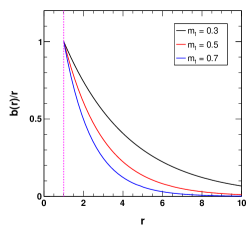
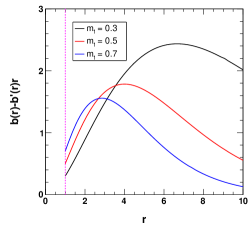
Figure 1: Plots of $b(r)/r$ vs. $r$ (on the left panel) and $b(r)-b^{\prime}(r)r$ vs. $r$ (on the right panel) for the wormhole shape function (17) with different values of the parameter $m_{1}$ and throat radius $r_{0}=1$. The vertical dotted line in each plot represents the position of the throat of the wormhole.

         

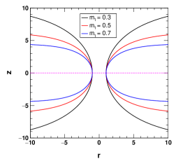
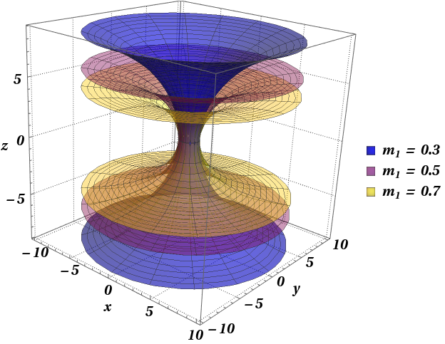
Figure 2: Embedded 2-D and 3-D plots of the wormhole defined by the shape function (17) with different values of the parameter $m_{1}$ and throat radius $r_{0}=1$.

         

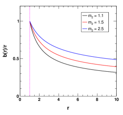
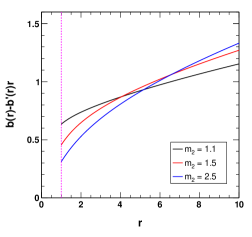
Figure 3: Plots of $b(r)/r$ vs. $r$ (on the left panel) and $b(r)-b^{\prime}(r)r$ vs. $r$ (on the right panel) for the wormhole shape function (18) with different values of the parameter $m_{2}$ and throat radius $r_{0}=1$. The vertical dotted line in each plot represents the position of the throat of the wormhole.

         

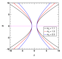
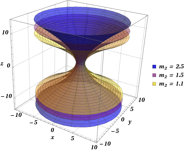
Figure 4: Embedded 2-D and 3-D plots of the wormhole defined by (18) with different values of the parameter $m_{2}$ and throat radius $r_{0}=1$.

         

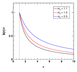
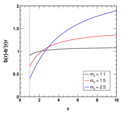
Figure 5: Plots of $b(r)/r$ vs. $r$ (on the left panel) and $b(r)-b^{\prime}(r)r$ vs. $r$ (on the right panel) for the wormhole shape function (19) with different values of the parameter $m_{3}$ and throat radius $r_{0}=1$. The vertical dotted line in each plot represents the position of the throat of the wormhole.

         

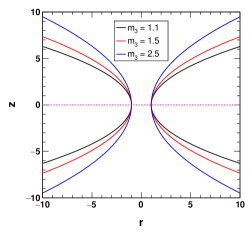
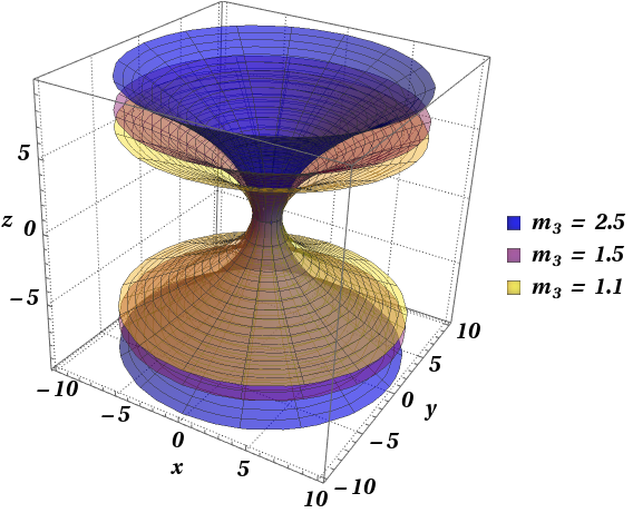
Figure 6: Embedded 2-D and 3-D plots of the wormhole defined by (19) with different values of the parameter $m_{3}$ and throat radius $r_{0}=1$.

Next, in order to visualise the embedded diagrams of the wormholes represented by toy shape functions (17), (18) and (19), we use an equatorial slice $\theta=\pi/2$ at a fixed time or at $t=$ constant. This gives us the privilege to reduce the metric (7) into the following form:

$$ds^{2}=\frac{dr^{2}}{1-b(r)/r}+r^{2}d\phi^{2}.$$ (20)

In cylindrical coordinates, we can write the above equation as

$$ds^{2}=dz^{2}+dr^{2}+r^{2}d\phi^{2}.$$ (21)

As the embedded surface in three dimensional Euclidean space is expressed by $z=z(r)$, we can rewrite Eq. (21) as

$$ds^{2}=\left[1+\left(dz/dr\right)^{2}\right]dr^{2}+r^{2}d\phi^{2}.$$ (22)

Finally, comparing the recasted metric (22) with the reduced metric (20), we get,

$$\dfrac{dz}{dr}=\pm\left[\dfrac{r}{b(r)}-1\right]^{-1/2}.$$ (23)

This relation gives the embedded surface of the wormhole. From the flare-out condition, we can see that the inverse of the embedding function $r(z)$ satisfies $d^{2}r/dz^{2}>0$ near or at the throat of the wormhole. More explicitly, differentiating inverse of the Eq. (23) with respect to $z$, we get,

$$\dfrac{d^{2}r}{dz^{2}}=\dfrac{b(r)-rb^{\prime}(r)}{2b(r)^{2}}>0.$$ (24)

Apart from this, from Eq. (23) one can see that $dz/dr\rightarrow\infty$ at the wormhole throat and the wormhole space is asymptotically flat as $r\rightarrow\infty$. Using Eq. (23) we have plotted the embedded diagrams of the wormholes in Fig.s 2, 4 and 6 for the toy shape functions (17), (18) and (19) respectively. These embedded diagrams show the impact of the model parameters on the shape of the wormhole. For the shape function (17) it is seen that with an increase in the model parameter $m_{1}$, height of the wormhole gets reduced. On the other hand, for the shape functions (18) and (19), it is clear from the diagrams 4 and 6 respectively that the impact of the model parameters $m_{2}$ and $m_{3}$ on the respective wormholes is similar in nature. In both cases, with an increase in the model parameters, the height of the wormholes increases gradually.

II.2 $f(R)$ gravity model from toy shape function of wormhole surrounded by a cloud of strings

Under some suitable conditions, it is possible to obtain the $f(R)$ gravity model for a wormhole shape function satisfying the field equations. Here, we shall consider the third toy shape function (19) as an example to obtain the corresponding $f(R)$ gravity model in presence of a cloud of strings. A cloud of strings is a kind of fluid model in which one-dimensional strings are distributed in a given direction, which may exist in different geometrical shapes, such as spherical, axisymmetric and planar Graca2018 . In our work we shall consider spherically symmetric cloud of strings distribution. The solution for a spherically symmetric strings cloud configuration was obtained in Ref. Graca2018 . The only non-null components of the energy-momentum tensor of a cloud of strings can be shown as

$$T^{t}_{t}=T^{r}_{r}=-\,\dfrac{\eta^{2}}{r^{2}},$$ (25)

where $\eta$ is a constant, which is related to the energy of the cloud of strings. For the shape function (19), the field Eq. (14) can be written as

$$\frac{(m_{3}^{2}-m_{3}\,r_{0})\mathcal{F}(r)}{r^{2}\left(m_{3}+r-r_{0}\right){}^{2}}+\frac{\eta^{2}}{r^{2}}=0.$$ (26)

Now, from this equation one can obtain an expression for $\mathcal{F}(r)$ given by

$$\mathcal{F}(r)=-\frac{\eta^{2}\left(m_{3}+r-r_{0}\right)^{2}}{m_{3}\left(m_{3}-r_{0}\right)}.$$ (27)

In this expression, $r$ can be replaced by the Ricci curvature using the definition (13) of Ricci curvature as

$$R=\frac{2m_{3}\left(m_{3}-r_{0}\right)}{r^{2}\left(m_{3}+r-r_{0}\right){}^{2}}.$$ (28)

Solving this equation for $r$ one can find,

$$r=\frac{1}{2}\left(\mp\,\sqrt{\left(m_{3}-r_{0}\right)^{2}\mp 4\sqrt{2\,m_{3}\left(m_{3}-r_{0}\right)/R}}-m_{3}+r_{0}\right).$$ (29)

For the mathematical feasibility we choose the solution given by

$$r=\frac{1}{2}\left(\sqrt{4\sqrt{2\,m_{3}\left(m_{3}-r_{0}\right)/R}+\left(m_{3}-r_{0}\right){}^{2}}-m_{3}+r_{0}\right).$$ (30)

One can obtain the throat radius of the wormhole in terms of background Ricci curvature using the limit $r\rightarrow r_{0}$ and $R\rightarrow R_{0}$ in the above Eq. (30). Using that relation for the throat radius, we have the final relation for $r$ as

$$r=\frac{A}{2\,m_{3}R_{0}}\left[\left\{4\sqrt{2}\,m_{3}^{2}R^{-1/2}\left(R_{0}/A\right)^{3/2}+1\right\}^{1/2}-1\right],$$ (31)

where $A=m_{3}^{2}R_{0}-\sqrt{2\,m_{3}^{2}R_{0}+1}+1$. Hence, Eq. (27) can be written as

$$\mathcal{F}(R)=-\,\frac{\eta^{2}A\left[1+\sqrt{1+4\sqrt{2}\,m_{3}^{2}R^{-1/2}\left(R_{0}/A\right)^{3/2}}\right]^{2}}{4\,m_{3}^{2}R_{0}}.$$ (32)

Integrating above expression with respect to $R$, we obtain the $f(R)$ function for the wormhole with the shape function (19) as

$$f(R) =-(2A^{2}m_{3}^{2}R_{0})^{-1}\eta^{2}\Bigg{[}\;\;\sqrt{A^{5}R\left(4\sqrt{2}m_{3}^{2}\sqrt{\frac{RR_{0}^{3}}{A}}+AR\right)}+4\sqrt{2}m_{3}^{2}\sqrt{A^{3}RR_{0}^{3}}$$ (33)

$$-8m_{3}^{4}R_{0}^{3}\log\left(\sqrt{A^{3}RR_{0}}+A\sqrt{R_{0}\left(4\sqrt{2}m_{3}^{2}R_{0}\sqrt{\frac{RR_{0}}{A}}+AR\right)}+2\sqrt{2}m_{3}^{2}R_{0}^{2}\right)+A^{3}R$$

$$+2Am_{3}^{3}R_{0}^{2}\sqrt{\frac{2AR}{m_{3}^{2}R_{0}}+8\sqrt{2}\sqrt{\frac{RR_{0}}{A}}}\;\;\Bigg{]}+C_{1}.$$

Here $C_{1}$ is an integration constant. In this function the background curvature is connected with the throat of the wormhole by the following relation:

$$R_{0}=\frac{2\left(m_{3}-r_{0}\right)}{m_{3}r_{0}^{2}}.$$ (34)

Obviously, the $f(R)$ function or model in Eq. (33) depends on the shape function of the wormhole. One may note that the cloud of strings parameter $\eta$ appears in the $f(R)$ model explicitly because of the presence of a cloud of strings in the wormhole spacetime as clear from our consideration above. Whereas the fact is that the shape function of the wormhole is considered to be independent of the cloud of strings parameter. In such a situation, the cloud of strings parameter contributes to the geometry modification only as shown in Eq. (33) and the basic properties of the wormhole remain independent of it. This type of situation arises when we define the shape function at first. So, for the toy shape functions of the wormholes, we shall not see any cloud of strings dependency with the quasinormal modes in general. Hence, such type of ad-hoc wormhole definitions may not be very feasible to study the impacts of any surrounding relics on the quasinormal modes from the wormhole spacetime. Any additional relic such as cloud of strings etc. will appear as a spacetime modification imprinted in the $f(R)$ gravity model due to fixing the shape function initially.

II.3 Wormhole solution in $f(R)$ gravity Starobinsky model surrounded by a cloud of strings

In this section, we shall obtain the wormhole solutions in $f(R)$ gravity Starobinsky model surrounded by a cloud of strings. Here the approach will be opposite to the previous case where we fixed the shape function at first and then calculated the corresponding $f(R)$ gravity model. This approach will help us obtain a wormhole shape function which has a dependency with the surrounding relic if any. In this work we shall use the Starobinsky’s inflationary model Starobinsky1980 , which is given by

$$f(R)=R+\alpha R^{2},$$ (35)

where $\alpha$ is the constant model parameter. Using this model (35) in Eq. (14), we obtain,

$$4\alpha b^{\prime}(r)^{2}+r^{2}b^{\prime}(r)+r^{2}\eta^{2}=0.$$ (36)

This equation can be solved for $b^{\prime}(r)$ as

$$b^{\prime}(r)=\frac{-\,r^{2}\pm r\,\sqrt{r^{2}-16\alpha\eta^{2}}}{8\alpha}.$$ (37)

For a feasible situation, we pick only the solution

$$b^{\prime}(r)=\frac{-\,r^{2}+r\,\sqrt{r^{2}-16\alpha\eta^{2}}}{8\alpha}$$ (38)

and the solution for $b(r)$ with the boundary condition $b(r_{0})=r_{0}$ yields,

$$b(r)=\frac{-\,r^{3}+\left(r^{2}-16\alpha\eta^{2}\right)^{3/2}-\left(r_{0}^{2}-16\alpha\eta^{2}\right){}^{3/2}+24\alpha r_{0}+r_{0}^{3}}{24\alpha}.$$ (39)

One may note that in this shape function of the wormhole, the cloud of strings parameter and $f(R)$ gravity model parameter appear explicitly and any modification in these parameters will affect the geometry of the wormhole and the corresponding quasinormal modes.

         

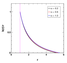
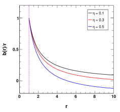
Figure 7: Plots of $b(r)/r$ vs. $r$ with $\eta=0.5$ (on the left panel) and with $\alpha=-0.10$ (on the right panel) for the wormhole shape function (39) with throat radius $r_{0}=1$. The vertical dotted line in each plot represents the position of the throat of the wormhole.

         

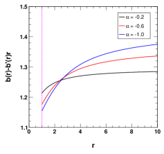
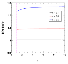
Figure 8: Plots of $b(r)-b^{\prime}(r)r$ vs. $r$ with $\eta=0.5$ (on the left panel) and with $\alpha=-0.10$ (on the right panel) for the wormhole shape function (39) with throat radius $r_{0}=1$. The vertical dotted line in each plot represents the position of the throat of the wormhole.

         

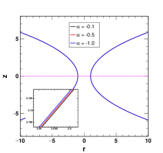
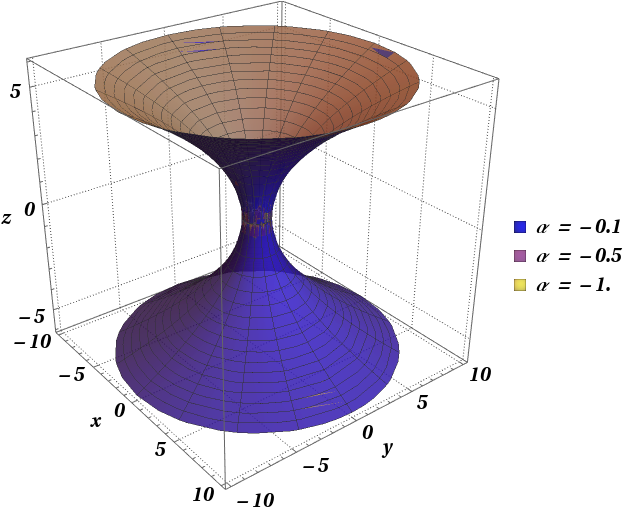
Figure 9: Embedded 2-D and 3-D plots of the wormhole defined by the shape function (39) with throat radius $r_{0}=1$ and $\eta=0.1$ for different values of $\alpha$.

         

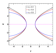
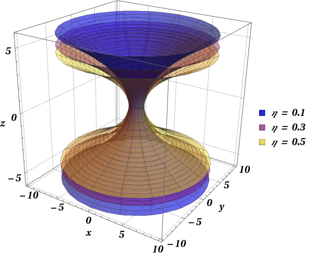
Figure 10: Embedded 2-D and 3-D plots of the wormhole defined by the shape function (39) with throat radius $r_{0}=1$ and $\alpha=-0.10$ for different values of $\eta$.

To check the viability of the new shape function (39), we have checked the necessary conditions mentioned earlier and two of the important conditions are shown in the Fig.s 7 and 8 for different values of shape function parameters $\alpha$ and $\eta$. In Fig. 7, we have plotted the function $b(r)/r$ vs. $r$ for different values of wormhole shape function parameters $\alpha$ and $\eta$. We see that the function shows a maximum value near the throat of the wormhole and it decreases gradually with an increase in the value of $r$ in both cases. Thus, clearly one can realise that $b(r)/r<1$ for $r>r_{0}$, which is a necessary condition for the formation of a wormhole. It is to be noted that here the impact of the Starobinsky model parameter $\alpha$ is very small in comparison to the cloud of strings parameter. In Fig. 8, we have plotted $b(r)-b^{\prime}(r)r$ vs. $r$ for the shape function for different values of $\alpha$ and $\eta$. The Starobinsky model parameter $\alpha$ shows a similar impact on the function $b(r)-b^{\prime}(r)r$ with the impacts of model parameters $m_{2}$ and $m_{3}$ of the toy shape functions defined in Eq. (18) and (19) respectively. With an increase in the values of $\alpha$, the function increases slowly and the value of the function is always greater than $0$. One may note that as previously mentioned for a viable wormhole, one needs $b(r)-b^{\prime}(r)r>0$. Moreover, the test function $b(r)-b^{\prime}(r)r$ and hence the shape function has a higher dependency on the other model parameter i.e. cloud of strings parameter $\eta$ as seen from the Fig. 8. Here also, the function is always greater than $0$ for any $r>r_{0}$ justifying the viability of the shape function (39). Now, to have a better visualisation of the wormhole shape function (39), we plot the embedded diagrams of the wormhole using the Eq. (23) after solving it numerically. The embedded diagrams are shown in Fig. 9 and in Fig. 10 for different values of the Starobinsky model parameter $\alpha$ and cloud of strings parameter $\eta$ respectively. From Fig. 9, one can see that the Starobinsky model parameter $\alpha$ has a very small impact on the structure of the wormhole as already clear from above. However, with decrease in $\alpha$, the height of the wormhole increases very slowly. Moreover, we have seen that for a viable wormhole one must have, $\alpha<0$. From these observations, we can infer that the Starobinsky model parameter has a very minimal impact over the structure of the wormhole. On the other hand, the cloud of strings parameter has a significant impact over the structure of the wormhole. As seen from the Fig. 10, with an increase in the cloud of strings parameter, the height of the wormhole decreases gradually. Hence, presence of a surrounding field e.g. a cloud of strings may have significant influences over different properties of the wormhole. The impact of these two model parameters on the quasinormal modes of wormhole will be elaborately studied in the next section.

II.4 Energy conditions

Here we shall study the energy conditions of the wormholes in $f(R)$ gravity metric formalism briefly. In GR, a fundamental requirement in wormholes is the violation of energy conditions Morris1988 ; Bolokhov2021 . Whereas in $f(R)$ theories of gravity, the required condition $R_{\mu\nu}k^{\mu}k^{\nu}\geq 0$ results null energy condition of the form $T^{eff}_{\mu\nu}k^{\mu}k^{\nu}\geq 0$ with the modified field equations. This expression can be used to study the NEC. Now, using a radial null vector, violation of NEC can be expressed as

$$\rho^{eff}+p_{r}^{eff}=\dfrac{\rho+p_{r}}{\mathcal{F}}+\dfrac{1}{\mathcal{F}}\left\{\mathcal{F}^{\prime\prime}\,\left(1-b(r)/r\right)-\mathcal{F}^{\prime}\,\left(b^{\prime}(r)r-b(r)\right)/(2r^{2})\right\}<0.$$ (40)

At the throat of the wormhole, this relation reduces to the following form:

$$\rho^{eff}+p_{r}^{eff}|_{r\,=\,r_{0}}=\dfrac{\rho+p_{r}}{\mathcal{F}}|_{r\,=\,r_{0}}+\dfrac{1-b^{\prime}(r_{0})}{2r_{0}}\dfrac{\mathcal{F}^{\prime}}{\mathcal{F}}|_{r\,=\,r_{0}}<0.$$ (41)

One may note that for a Morris-Throne wormhole in GR, the flare out condition is sufficient to yield a violation of the NEC at the throat. It can be easily checked by using $\mathcal{F}=1$ in Eq.s (14) and (15) that

$$\rho(r_{0})+p_{r}(r_{0})=\dfrac{r_{0}b^{\prime}(r_{0})-b(r_{0})}{b(r_{0})^{2}\,r_{0}}<0,$$ (42)

as we have $b(r_{0})=r_{0}$ at the throat of the wormhole. But from Eq. (40) one can see that in $f(R)$ gravity, the violation of NEC depends on the form of the $f(R)$ gravity model also apart from the shape function.

         

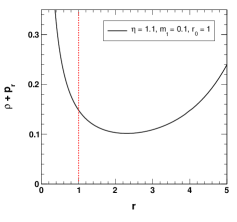
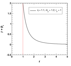
Figure 11: Variation of $\rho+p_{r}$ for shape function (17) (on left) and (18) (on right).

         

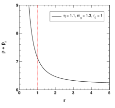
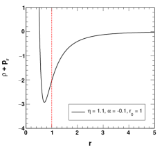
Figure 12: Variation of $\rho+p_{r}$ for shape function (19) (on left) and (39) (on right).

Now we shall study the NEC for our toy shape functions and the Starobinsky model. Since $\rho(r)+p_{r}(r)$ has a complex form, we shall see the condition only at the throat for simplicity. So at the throat of the wormhole, the first toy shape function defined in Eq. (17) gives,

$$\rho(r_{0})+p_{r}(r_{0})=-\frac{\eta^{2}m_{1}\left(m_{1}^{2}r_{0}^{2}-2\right)}{2r_{0}\left(m_{1}r_{0}-1\right)^{2}}.$$ (43)

From this expression, it is found that the wormhole solution violates NEC for $(m_{1}r_{0}>\sqrt{2})\;\cup\;(-\frac{\sqrt{2}}{r_{0}}<m_{1}<0)$ and beyond this range the solution respects the NEC. For the second shape function defined by Eq. (18), we have at the throat of the wormhole,

$$\rho(r_{0})+p_{r}(r_{0})=\frac{\eta^{2}\Big{[}\log\left(2m_{2}r_{0}\right)\Big{\{}8\log\left(2m_{2}r_{0}\right)-1\Big{\}}-2\Big{]}}{4\log\left(2m_{2}r_{0}\right)\Big{\{}r_{0}-2r_{0}\log\left(2m_{2}r_{0}\right)\Big{\}}^{2}}.$$ (44)

NEC is violated at the throat for the following range:

$$\log\left(2m_{2}r_{0}\right)<\frac{1}{16}\left(1-\sqrt{65}\right)\;\cup\;0<\log\left(2m_{2}r_{0}\right)<\frac{1}{16}\left(\sqrt{65}+1\right)$$ (45)

and beyond this range the NEC is respected. Similarly, for the third shape function defined in Eq. (19), at the throat of the wormhole,

$$\rho(r_{0})+p_{r}(r_{0})=\frac{\eta^{2}\left(m_{3}+r_{0}\right)}{m_{3}r_{0}\left(m_{3}-r_{0}\right)}.$$ (46)

In this case the NEC is violated for $0<m_{3}<r_{0}\;\cup\;m_{3}+r_{0}<0.$ Finally for the Starobinsky model case, we have

$$\rho(r_{0})+p_{r}(r_{0})=\frac{4\alpha\eta^{2}\left(\sqrt{r_{0}^{2}-16\alpha\eta^{2}}+2\eta^{2}r_{0}+r_{0}\right)}{r_{0}^{3}\left(-16\alpha\eta^{2}-r_{0}\sqrt{r_{0}^{2}-16\alpha\eta^{2}}+r_{0}^{2}\right)}.$$ (47)

In this situation the NEC is violated for $(\alpha<0)\;\cup\;(0<\alpha<\frac{r_{0}^{2}}{16\eta^{2}}).$ Moreover, one may note that for $\alpha>\frac{r_{0}^{2}}{16\eta^{2}}$, Eq. (47) results in imaginary values. Hence, for this case, NEC is violated for the complete feasible range in the parameter space.

We have also checked the NEC for the variable $r$ graphically in Fig.s 11 and 12 for the shape functions (17), (18), (19) and (39) respectively for selected set of parameters. Since the expressions for $\rho+p_{r}$ are complex, we have given their explicit forms along with the corresponding $df(R)/dR$ in terms of $r$ in the appendix. On the left panel of Fig. 11, we have shown the variation of NEC for the first wormhole shape function with $\eta=1.1$, $m_{1}=0.1$ and the throat radius of the wormhole $r_{0}=1$. The red dotted line represents the throat of the wormhole. One may note that for the chosen value of the parameters, NEC is respected at the throat of the wormhole. With an increase in the distance from the throat of the wormhole, $\rho+p_{r}$ increases gradually respecting NEC. On the right panel of Fig. 11, we have shown the variation of $\rho+p_{r}$ for the second wormhole shape function defined by (18) with the model parameters $\eta=1.1$, $m_{2}=1.2$ and the throat radius of the wormhole $r_{0}=1$. In this case also, the selected values of the parameters respect the NEC at the throat as seen from the previous results. From the figure, one can see that in this case $\rho+p_{r}$ is positive at the throat of the wormhole and gradually decreases towards $0$ with an increase in $r$.

On the left panel of Fig. 12, we have shown variation of $\rho+p_{r}$ for the third shape function defined by (19). In this case we have chosen $\eta=1.1$, $m_{3}=1.3$ and the throat radius of the wormhole $r_{0}=1$. These values of the parameters respect the NEC at the throat of the wormhole. We have seen that with an increase in the value of $r$, $\rho+p_{r}$ decreases gradually but the value of $\rho+p_{r}$ is much greater than $0$ for this particular shape function. Finally, on the right panel of Fig. 12, we have shown the variation of $\rho+p_{r}$ with respect to $r$ for the shape function obtained for the Starobinsky $f(R)$ gravity model surrounded by a cloud of strings. We have already seen that for the feasible $\alpha<0$ values and at the throat, this wormhole always violates the NEC. Hence, with the selected values of the model parameters $\eta=1.1$, $\alpha=-0.1$ and $r_{0}=1$, we have seen that $\rho+p_{r}$ violates NEC for a variable $r$ and with an increase in the value of $r$, $\rho+p_{r}$ approaches to $0$ gradually.

So, as a result we have seen that the wormhole solution obtained in $f(R)$ gravity Starobinsky model always violates NEC, while the three toy shape functions can violate NEC in a particular range of the model parameters only. This range has been calculated explicitly at the throat of the wormholes for each of toy shape function.

III Quasinormal modes

Quasinormal modes of compact stellar objects, such as black holes, wormholes etc. are the long lasting components of gravitational waves from such objects when the morphological symmetry of those objects are disturbed by some perturbative effects. Quasinormal mode frequencies are usually expressed in terms of complex numbers, where the real part represents the amplitude of the mode and the imaginary part represents the loss of energy of the objects. Thus by quasinormal modes compact objects try to regain their original state with the loss of energies. The details about the quasinormal modes can be found in Ref.s Kokkotas ; Vishveshwara ; Press ; Chandrasekhar ; Berti2015 ; Dreyer2004 ; Chen ; Zhang ; Zhang2 ; Ma ; Zhang3 ; Graca . To calculate the quasinormal mode frequencies of a compact object it is necessary to use an external field surrounding the object as a probe, which can give a measure of the perturbation in the object. There are various possible probe fields, e.g. scalar fields, vector fields, fermionic or Dirac fields Frolov2018 ; Jing2005 ; Chowdhury2018 etc. surrounding the compact objects. Here, we shall study the quasinormal modes from the wormholes for the scalar (field) perturbations and Dirac (field) perturbations using WKB approximation method. We shall neglect any possible echoes from quantum corrections near the wormhole throat or from any matter far from it Konoplya2018 ; Konoplya2022 .

The primary problem in the quasinormal modes calculations of wormholes is related with the potential, because in the absence of tidal forces and in the usual situation, the peak of the potential is at the throat of the wormhole. In normal coordinates it is difficult to visualise such peak of the potential properly. This issue can be simply avoided by converting the potential of the problem into tortoise coordinates. During the calculations, we assume that the test fields such as scalar field or Dirac field have negligible reaction on the spacetime.

III.1 Scalar Perturbation

Now we consider a massless scalar field $\zeta$ around the wormhole spacetime. Assuming that the reaction of the scalar field on the spacetime negligible as mentioned above, it is possible to describe the quasinormal modes of the wormholes by the Klein Gordon equation in curved spacetime as given by

$$\square\zeta=\dfrac{1}{\sqrt{-g}}\partial_{\mu}(\sqrt{-g}g^{\mu\nu}\partial_{\nu}\zeta)=0.$$ (48)

Using spherical harmonics, it is possible to decompose the scalar field in the following form:

$$\zeta(t,r,\theta,\phi)=\dfrac{1}{r}\sum_{l,m}\psi_{l}(t,r)Y_{lm}(\theta,\phi),$$ (49)

where $\psi_{l}(t,r)$ is the radial time dependent wave function, and $l$ and $m$ are the indices of the spherical harmonics. Using this equation in (48), we get,

$$\partial^{2}_{r_{*}}\psi(r_{*})_{l}+\omega^{2}\psi(r_{*})_{l}=V_{s}(r)\psi(r_{*})_{l},$$ (50)

where $r_{*}$ is the tortoise coordinate defined by

$$\dfrac{dr_{*}}{dr}=\sqrt{\frac{r\;e^{-2\phi(r)}}{r-b(r)}}$$ (51)

and the effective potential is given by

$$V_{s}(r)=\frac{e^{2\Phi(r)}\left[-\,rb^{\prime}(r)+b(r)\left(1-2r\Phi^{\prime}(r)\right)+2r\left\{l(l+1)+r\Phi^{\prime}(r)\right\}\right]}{2r^{3}}.$$ (52)

Here $l$ is referred to as the multipole moment of the quasinormal modes of the wormhole.

III.2 Dirac Perturbation

For the perturbation of Dirac field with mass $m$, one can write the general equation as Brill1957 ; Cho2003

$$[\gamma^{a}e_{a}^{\mu}(\partial_{\mu}+\Gamma_{\mu})+m]\psi=0,$$ (53)

where $\Gamma_{\mu}=\frac{1}{8}[\gamma^{a},\gamma^{b}]e_{a}^{\nu}e_{b\nu;\mu}$ is the spin connection, $\gamma^{a}$ are the Dirac metrices and $e_{b\nu;\mu}=\partial_{\mu}e_{b\nu}-\Gamma_{\mu\nu}^{\alpha}e_{b\alpha}$. Using our ansatz (7), $e_{\nu}^{a}$ can be taken to be

$$e_{\nu}^{a}={\rm diag}(e^{\Phi(r)},(1-b(r)/r)^{-1/2},r,r\sin\theta).$$ (54)

Using this and now considering massless Dirac field i.e. $m=0$, Eq. (53) can be further written in the following form:

$$\partial^{2}_{r_{*}}\psi(r_{*})_{l}+\omega^{2}\psi(r_{*})_{l}=V_{d\pm}(r)\psi(r_{*})_{l},$$ (55)

where $r_{*}$ is the tortoise coordinate and two isospectral potentials,

$$V_{d\pm}(r)=\frac{k}{r}\left(\frac{ke^{2\Phi(r)}}{r}\mp\frac{e^{2\Phi(r)}\sqrt{(1-b(r)/r)}}{r}\pm e^{\Phi(r)}\sqrt{(1-b(r)/r)}\dfrac{d\;e^{\Phi(r)}}{dr}\right).$$ (56)

Here $k=1,2,3\ldots$ are called the multipole numbers with $k=\ell+1/2$. The potentials can be transformed from one to another form by using the Darboux transformation as shown below:

$$\psi_{+}=A\left(W+\dfrac{d}{dr_{*}}\right)\psi_{-},\quad W=\sqrt{e^{\Phi(r)}\sqrt{(1-b(r)/r)}},$$ (57)

where $A$ is a constant. As $+$ and $-$ wave equations are isospectral, we shall consider only one of the two effective potentials for the Dirac case.

III.3 WKB method for Quasinormal modes

The first order WKB method for calculating the quasinormal modes was first suggested by Schutz and Will in Schutz . Later, the method was developed to higher orders Will_wkb ; Konoplya_wkb ; Maty_wkb . In this work, we shall use higher order WKB methods, more specifically the 3rd order and 5th order WKB approximation methods to calculate the quasinormal modes from the wormholes defined in the previous sections.

Table 1: Fundamental quasinormal modes of the wormhole defined by the shape function (17) for the scalar perturbation with $m_{1}=0.3$ and $r_{0}=1$.

$l$	WKB $3$rd order	WKB $5$th order	$\Delta_{3}$	$\Delta_{5}$
$l=1$	$1.4317-0.1853i$	$1.4322-0.1851i$	$0.000863134$	$0.000111803$
$l=2$	$2.4434-0.1862i$	$2.4435-0.1862i$	$0.000280943$	$0.0000132872$
$l=3$	$3.4426-0.1864i$	$3.4427-0.1864i$	$0.000139003$	$3.40181\times 10^{-6}$
$l=4$	$4.4378-0.1865i$	$4.4378-0.1865i$	$0.0000830125$	$1.23455\times 10^{-6}$

Table 2: Fundamental quasinormal modes of the wormhole defined by the shape function (17) for the Dirac perturbation with $m_{1}=0.3$ and $r_{0}=1$.

$k$	WKB $3$rd order	WKB $5$th order	$\Delta_{3}$	$\Delta_{5}$
$k=8$	$7.9443-0.1882i$	$7.9455-0.1697i$	$0.000801561$	$0.12791$
$k=9$	$8.9348-0.1880i$	$8.9356-0.1777i$	$0.000502494$	$0.0628711$
$k=10$	$9.9252-0.1879i$	$9.9257-0.1817i$	$0.00035$	$0.0334861$
$k=11$	$10.9155-0.1877i$	$10.9159-0.1839i$	$0.00025$	$0.0189136$

Table 3: Fundamental quasinormal modes of the wormhole defined by the shape function (18) for the scalar perturbation with $m_{2}=1.3$ and $r_{0}=1$.

$l$	WKB $3$rd order	WKB $5$th order	$\Delta_{3}$	$\Delta_{5}$
$l=1$	$1.45101-0.251715i$	$1.45255-0.25038i$	$0.00181116$	$0.000638004$
$l=2$	$2.45502-0.247206i$	$2.45537-0.247046i$	$0.000629713$	$0.0000668254$
$l=3$	$3.45096-0.246039i$	$3.45109-0.245998i$	$0.000318384$	$0.0000163396$
$l=4$	$4.44427-0.245568i$	$4.44434-0.245553i$	$0.000191903$	$5.81055\times 10^{-6}$

Table 4: Fundamental quasinormal modes of the wormhole defined by the shape function (18) for the Dirac perturbation with $m_{2}=1.3$ and $r_{0}=1$.

$k$	WKB $3$rd order	WKB $5$th order	$\Delta_{3}$	$\Delta_{5}$
$k=10$	$9.9313-0.2489i$	$9.9421-0.0908i$	$0.00676849$	$1.29907$
$k=11$	$10.9219-0.2483i$	$10.9293-0.1497i$	$0.00461736$	$0.683984$
$k=12$	$11.9124-0.2479i$	$11.9178-0.1839i$	$0.00326382$	$0.395367$
$k=13$	$12.9028-0.2475i$	$12.9068-0.2045i$	$0.00241299$	$0.241984$

Table 5: Fundamental quasinormal modes of the wormhole defined by the shape function (19) for the scalar perturbation with $m_{3}=1.3$ and $r_{0}=1$.

$l$	WKB $3$rd order	WKB $5$th order	$\Delta_{3}$	$\Delta_{5}$
$l=1$	$1.47458-0.308873i$	$1.47748-0.305617i$	$0.00307541$	$0.00168329$
$l=2$	$2.46893-0.301043i$	$2.46966-0.300633i$	$0.00110078$	$0.000177451$
$l=3$	$3.46087-0.298982i$	$3.46114-0.298877i$	$0.000561802$	$0.0000431066$
$l=4$	$4.45198-0.298148i$	$4.45211-0.298109i$	$0.000339966$	$0.0000152743$

Table 6: Fundamental quasinormal modes of the wormhole defined by the shape function (19) for the Dirac perturbation with $m_{3}=1.3$ and $r_{0}=1$.

$k$	WKB $3$rd order	WKB $5$th order	$\Delta_{3}$	$\Delta_{5}$
$k=13$	$12.9085-0.3013i$	$12.9185-0.1644i$	$0.00627415$	$0.988848$
$k=14$	$13.899-0.3008i$	$13.9066-0.2060i$	$0.00467172$	$0.615035$
$k=15$	$14.8895-0.3004i$	$14.8953-0.2331i$	$0.00357246$	$0.400761$
$k=16$	$15.8799-0.3001i$	$15.8845-0.2512i$	$0.00277218$	$0.270291$

Table 7: Fundamental quasinormal modes of the wormhole in Starobinsky model defined by the shape function (39) for the scalar perturbation with $\alpha=-0.3$, $\eta=0.5$ and $r_{0}=1$.

$l$	WKB $3$rd order	WKB $5$th order	$\Delta_{3}$	$\Delta_{5}$
$l=1$	$1.50652-0.401418i$	$1.51379-0.389575i$	$0.00693889$	$0.00702422$
$l=2$	$2.49009-0.381394i$	$2.492-0.380002i$	$0.00230204$	$0.000643374$
$l=3$	$3.47658-0.375938i$	$3.47729-0.375589i$	$0.00114282$	$0.000147775$
$l=4$	$4.46441-0.373693i$	$4.46474-0.373568i$	$0.000682844$	$0.0000511278$

Table 8: Fundamental quasinormal modes of the wormhole in Starobinsky model defined by the shape function (39) for the Dirac perturbation with $\alpha=-0.3$, $\eta=0.5$ and $r_{0}=1$.

$k$	WKB $3$rd order	WKB $5$th order	$\Delta_{3}$	$\Delta_{5}$
$k=16$	$15.8877-0.376659i$	$15.9049-0.143713i$	$0.0105442$	$1.77187$
$k=17$	$16.8783-0.376026i$	$16.8918-0.203532i$	$0.00829676$	$1.18099$
$k=18$	$17.8688-0.375502i$	$17.8796-0.245583i$	$0.00661801$	$0.819652$
$k=19$	$18.8592-0.375063i$	$18.8681-0.275713i$	$0.0053437$	$0.585226$

         

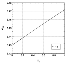
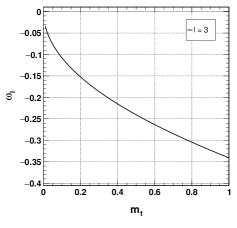
Figure 13: Variation of the fundamental scalar quasinormal modes with model parameter $m_{1}$ for the wormhole defined by the shape function (17), calculated with 3rd order WKB approximation method.

         

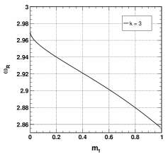
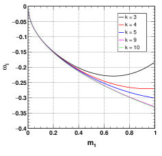
Figure 14: Variation of the fundamental Dirac quasinormal modes with model parameter $m_{1}$ for the wormhole defined by the shape function (17), calculated with 3rd order WKB approximation method.

         

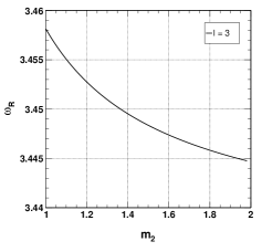
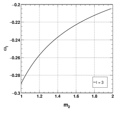
Figure 15: Variation of the fundamental scalar quasinormal modes with model parameter $m_{2}$ for the wormhole defined by the shape function (18), calculated with 3rd order WKB approximation method.

         

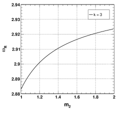
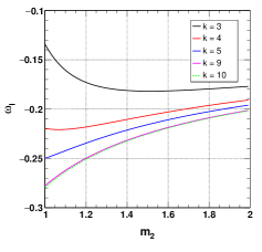
Figure 16: Variation of the fundamental Dirac quasinormal modes with model parameter $m_{2}$ for the wormhole defined by the shape function (18), calculated with 3rd order WKB approximation method.

         

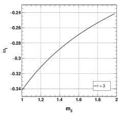
Figure 17: Variation of the fundamental scalar quasinormal modes with model parameter $m_{3}$ for the wormhole defined by the shape function (19), calculated with 3rd order WKB approximation method.

         

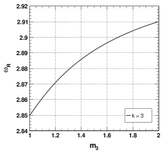
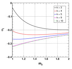
Figure 18: Variation of the fundamental Dirac quasinormal modes with model parameter $m_{3}$ for the wormhole defined by the shape function (19), calculated with 3rd order WKB approximation method.

         

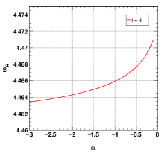
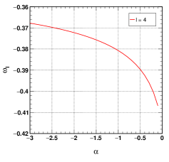
Figure 19: Variation of the fundamental scalar quasinormal modes with model parameter $\alpha$ for the wormhole defined by the shape function (39), calculated with 3rd order WKB approximation method using $\eta=0.7$ and $r_{0}=1$.

         

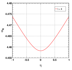
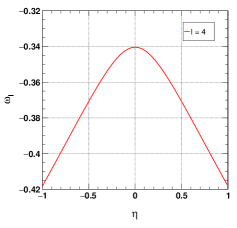
Figure 20: Variation of the fundamental scalar quasinormal modes with model parameter $\eta$ for the wormhole defined by the shape function (39), calculated with 3rd order WKB approximation method using $\alpha=-0.5$ and $r_{0}=1$.

         

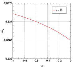
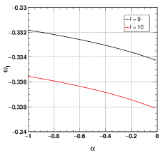
Figure 21: Variation of the fundamental Dirac quasinormal modes with model parameter $\alpha$ for the wormhole defined by the shape function (39), calculated with 3rd order WKB approximation method using $\eta=0.3$ and $r_{0}=1$.

         

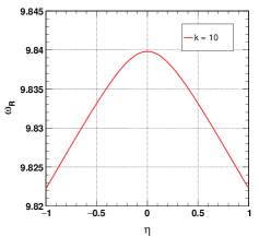
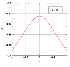
Figure 22: Variation of the fundamental Dirac quasinormal modes with model parameter $\eta$ for the wormhole defined by the shape function (39), calculated with 3rd order WKB approximation method using $\alpha=-0.5$ and $r_{0}=1$.

At first, we calculated the quasinormal modes for scalar perturbation for the wormhole defined by the shape function (17) using $m_{1}=0.3$ and throat $r_{0}=1$. The value of the parameter $m_{1}$ is chosen in such a way that it satisfies the viability conditions for a wormhole mentioned earlier. The results for different multipole numbers are shown in Table 1. In this table and following ones $\Delta_{3}$ is defined as

$$\Delta_{3}=\dfrac{\vline\;\omega_{4}-\omega_{2}\;\vline}{2},$$ (58)

and similarly,

$$\Delta_{5}=\dfrac{\vline\;\omega_{6}-\omega_{4}\;\vline}{2},$$ (59)

where $\omega_{2},\omega_{4}$ and $\omega_{6}$ represent the quasinormal modes obtained from 2nd order, 4th order and 6th order WKB approximation methods respectively. $\Delta_{3}$ and $\Delta_{5}$ give a measurement of the errors associated with the quasinormal modes obtained from 3rd order and 5th order WKB approximation methods. It is clearly visible from the Table 1 that with an increase in $l$, magnitudes of both the real and imaginary frequencies increase gradually. So, for higher multipole numbers the decay rate of the quasinormal frequency increases slowly. Another point to note is that the corresponding errors also decrease as the value of $l$ increases. In this case, 5th order WKB method seems to be more accurate with less errors. For the same wormhole, we have calculated the Dirac quasinormal modes in Table 2. In this scenario, for lower $k$ values, the WKB approximation gives less accurate results due to the behaviour of the corresponding potentials. Hence, we have listed the quasinormal modes for some higher values of $k$. In this case, considering the 3rd order WKB results which have less errors, with an increase in the value of $k$, we observe a decrease in the decay rate of the quasinormal frequencies while the real part increases gradually following the previous trend of scalar perturbation. One may note that in case of Dirac perturbation, 5th order WKB method is less accurate in comparison to the 3rd order WKB method. The errors, as expected, decrease with increase in the value of $k$. Similarly, we have calculated the quasinormal modes for the second wormhole (18) and listed them in Table 3 for scalar perturbation. In this case, with an increase in the multipole number $l$, the decay rate decreases following an opposite trend in comparison to the first case. For this wormhole, the Dirac quasinormal modes are listed in Table 4. For the third wormhole, defined by Eq. (19), the scalar and Dirac quasinormal modes are listed in Tables 5 and 6 respectively. For this case also, the scalar quasinormal modes decrease with an increase in the value of $l$.

To get a clear picture, we have plotted the real and imaginary quasinormal modes of the wormhole (17) with respect to the model parameter $m_{1}$ in Fig. 13 for scalar perturbations and in Fig. 14 for Dirac perturbations using 3rd order WKB approximation method. The reason for choosing 3rd order WKB method in the plots can be justified from the previous tables, where we have seen that in general the 5th order WKB method results in higher magnitudes of errors basically in Dirac perturbations. In Fig. 13, it is seen that the real quasinormal mode increases linearly with respect to the model parameter $m_{1}$. However, at the same time, the decay rate also increases following a non-linear pattern. The decay rate is smaller when the parameter $m_{1}$ negligibly small. The Dirac quasinormal modes are shown in Fig. 14. The real quasinormal modes decrease with an increase in the model parameter $m_{1}$. However, in case of decay rates, we observe a multipole dependency towards $m_{1}=1$. Initially, for all multipole modes, decay rate increases with an increase in $m_{1}$. But, for smaller multipole modes, a reverse pattern is observed near $m_{1}=1$. The decay rates for $l=3$ start increasing gradually near $m_{1}=1$. In the case of $l=4$, the slope of the decay rate curve becomes very small near $m_{1}=1$. However, for higher multipole modes, such a pattern vanishes and the decay rates become almost identical to each other.

We have shown the variation of the scalar quasinormal modes for the second shape function defined by Eq. (18) in Fig. 15. Here, we have chosen the range of the parameter $m_{2}$ in such a way that the shape function satisfies the viability conditions. It is seen that an increase in the parameter from $m_{2}=1$ to $2$ results in decrease of the quasinormal frequencies and at the same time the decay rate also decreases gradually. In case of Dirac quasinormal modes (see Fig. 16), however, an increase in the parameter $m_{2}$ results in an increase of the quasinormal frequencies. But in decay rate, we observe an anomalous pattern which depends on the multipole number $l$. For $l=3$, the decay rate initially increases with an increase in $m_{2}$ and beyond $m_{2}=1.4$, the decay rate starts to decrease very slowly with an increase in $m_{2}$. For $l=4$, decay rate increases very slowly near $m_{2}=1.1$ and beyond this, decay rate decreases. In the case of $l=5$ and above, the decay rate only decreases gradually from $m_{2}=1$ to $2$. It may be noted that for higher $l$ values, the decay rates are almost identical to each other and they start decreasing with an increase in $m_{2}$ beyond $1$. For the third shape function (19) also, the scalar quasinormal modes follow a similar pattern to that of the second shape function as seen from the Fig. 17. In case of the Dirac quasinormal modes as seen from Fig. 18, the quasinormal frequencies increase with increase in the parameter $m_{3}$ and the decay rate follows a similar trend as that of the Dirac perturbation case for the shape function (18). Hence, the analysis shows that the shape functions (18) and (19) show a similar behaviour in terms of the quasinormal modes of the wormholes in both scalar and Dirac quasinormal modes.

We now move to the new shape function that has been obtained from the Starobinsky $f(R)$ gravity model surrounded by a cloud of strings. We have calculated the quasinormal modes for different values of multipole moments in Tables 7 and 8 for the scalar and Dirac perturbations respectively. In this case also, we observe that the errors associated with the scalar perturbation are comparatively smaller than those found in the Dirac perturbation. In the scalar perturbation, 5th order WKB has smaller errors. The real quasinormal mode increases and the decay rate decreases with an increase in the value of multipole moment, $l$. In the case of Dirac perturbation also, with an increase in $k$, real quasinormal mode increases. But according to the results from 3rd WKB, the decay rate decreases and for 5th WKB, decay rate increases with an increase in $k$. However, one may note that the errors associated with 5th order WKB are higher and this is basically due to the form of the potential. For smaller values of $k$, the errors are large. Since, the error associated with 3rd order WKB is comparatively smaller, we can use the trend provided by this method for the implications from quasinormal modes. Moreover, we use 3rd order WKB in case of this new shape function also, in order to analyse the quasinormal modes graphically. For this shape function defined by (39), we have observed the variation of real and imaginary quasinormal modes with respect to the Starobinsky model parameter $\alpha$ in Fig. 19. The real quasinormal modes increase non-linearly with an increase in the parameter $\alpha$ towards $0$. One may note that it is not possible to obtain a wormhole solution and hence the corresponding quasinormal modes for positive values of the parameter $\alpha$. The decay rate also increases non-linearly with an increase in the parameter $\alpha$. In Fig. 20, we have shown the dependency of the scalar quasinormal frequencies and the decay rates with respect to the cloud of strings parameter present in the wormhole shape function. It is obvious from the figure that he quasinormal frequencies and the decay rates depend on the magnitude of the parameter $\eta$ only. With a decrease in the magnitude of the parameter $\eta$ towards $0$, both the quasinormal frequencies and the decay rates decrease to a minimum value.

The variation of Dirac quasinormal modes with respect to the parameter $\alpha$ for the wormhole obtained in the Starobinsky model is shown in Fig. 21. In this case, the real quasinormal modes decrease with an increase in $\alpha$. The decay rate, on the other hand, increases with an increase in $\alpha$. So, in both types of perturbations, i.e. in scalar and Dirac perturbations, an increase in the Starobinsky parameter, the decay rate increases.

Finally, we have plotted the real and imaginary Dirac quasinormal modes with respect to $\eta$ for the wormhole in the Starobinsky model in Fig. 22. It is seen that an increase in the magnitude of $\eta$, decreases the quasinormal frequencies gradually. On the other hand, the decay rate increases with an increase in the magnitude of $\eta$. So, in general for both the type of perturbations, i.e. for the scalar and Dirac perturbations $\eta$ has a similar type of impact over the decay rate of the quasinormal frequencies, while the impact of $\eta$ over the real quasinormal modes is opposite.

IV Time Domain Analysis

We study the evolution of the scalar and Dirac perturbations, especially the time domain profiles for these perturbations in this section for the considered wormhole solutions. To study the time domain profiles for the respective perturbation schemes we implement the time domain integration method introduced in Ref. gundlach . We define the associated wavefunction as $\psi(r_{*},t)=\psi(i\Delta r_{*},j\Delta t)\equiv\psi_{i,j}$ and the potential as $V(r(r_{*}))=V(r_{*},t)\equiv V_{i,j}$ to write Eq. (48) in the form:

$$\dfrac{\psi_{i+1,j}-2\psi_{i,j}+\psi_{i-1,j}}{\Delta r_{*}^{2}}-\dfrac{\psi_{i,j+1}-2\psi_{i,j}+\psi_{i,j-1}}{\Delta t^{2}}-V_{i}\psi_{i,j}=0.$$ (60)

         

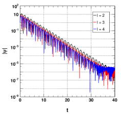
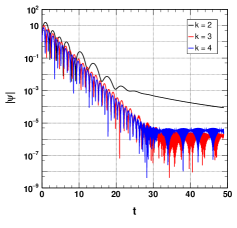
Figure 23: Time domain profile for the wormhole defined by the shape function (39) for the scalar perturbation with $\alpha=-0.5$, $\eta=0.1$ and $r_{0}=1$ (on the left panel) and for the Dirac perturbation with $\alpha=-0.3,\eta=0.5$ and $r_{0}=1$ (on the right panel).

         

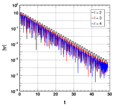
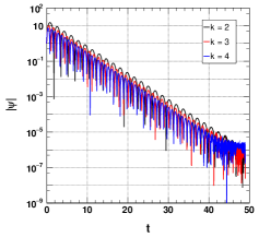
Figure 24: Time domain profile for the wormhole defined by the shape function (17) for the scalar perturbation (on the left panel) and the Dirac perturbation (on the right panel) with $m_{1}=0.5$ and $r_{0}=1$.

         

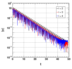
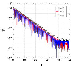
Figure 25: Time domain profile for the wormhole defined by the shape function (18) for the scalar perturbation (on the left panel) and the Dirac perturbation (on the right panel) with $m_{2}=1.1$ and $r_{0}=1$.

         

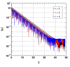
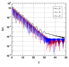
Figure 26: Time domain profile for the wormhole defined by the shape function (19) for the scalar perturbation (on the left panel) and the Dirac perturbation (on the right panel) with $m_{3}=1.1$ and $r_{0}=1$.

Identifying the initial conditions as $\psi(r_{*},t)=\exp\left[-\dfrac{(r_{*}-k_{1})^{2}}{2\sigma^{2}}\right]$ and $\psi(r_{*},t)|_{t<0}=0$ (here $k_{1}$ and $\sigma$ are median and width of the initial wave-packet), it is possible to express the time evolution of the scalar field as

$$\psi_{i,j+1}=-\psi_{i,j-1}+\left(\dfrac{\Delta t}{\Delta r_{*}}\right)^{2}(\psi_{i+1,j+\psi_{i-1,j}})+\left(2-2\left(\dfrac{\Delta t}{\Delta r_{*}}\right)^{2}-V_{i}\Delta t^{2}\right)\psi_{i,j}.$$ (61)

In order to comply with the Von Neumann stability condition we have chosen $\frac{\Delta t}{\Delta r_{*}}<1$ during the numerical procedure. We use the same method for the Dirac perturbation scheme also to obtain the time domain profiles or the time evolution of the perturbations for a selected set of parameters. The time profiles for scalar and Dirac perturbations are shown in Fig.s 23, 24, 25 and 26 for shape function obtained from Starobinsky model and toy shape functions respectively. The profiles show that with an increase in the number of the multipole modes, the oscillation frequency increases. Another important implication is that the corresponding oscillation frequency for the Dirac perturbation case is smaller than that obtained for the scalar perturbation. The damping rate or decay rate also increases slowly with an increase in the multipole modes for both types of perturbations. One may also note that the times domain profiles for the Starobinsky model case are distinguishable from the time domain profiles of the toy wormhole models. It is because of the impact of the cloud of strings parameter. In the Starobinsky model case, the structure of the wormhole highly depends on the surrounding cloud of strings and any variation in the cloud of strings parameter will impact the quasinormal modes and time domain profiles obtained from the perturbation of the wormhole geometry. But in case of the toy models, we have well defined the shape functions initially and hence the cloud of strings parameter appears as a contribution towards the geometry modification i.e. the corresponding $f(R)$ gravity model has the cloud of strings parameter as a model parameter in it. This basically provides an $f(R)$ gravity model which can compensate the effect of cloud of strings for the chosen shape function of the wormhole. In Fig. 24, for both type of perturbations we have chosen $m_{1}=0.5$ and throat radius of the wormhole $r_{0}=1$. Similar to the previous case, we observe that with increase in the multipole moment, quasinormal frequencies and decay rate increases. However, the variation of decay rate is comparatively small. In Fig.s 25 and 26, we have used $m_{2}=1.1$ and $m_{3}=1.1$ respectively. We observe that for both cases, the time domain profiles are not identical and the variation is more prominent in case of the Dirac perturbation. These results support the previous results obtained from the WKB analysis. So, at last we can summarise that the structure of the wormholes are connected with the quasinormal modes and hence also on the time domain profiles. Next generation GWs detectors like LISA may play a prominent role Gogoi_bumblebee in distinguishing between quasinormal modes from black holes and wormholes and hopefully may be able to constrain the wormhole shape functions to a satisfactory order.

However, one can also consider constraining the gravity models using cosmological or other experimental data to see how tightly the quasinormal spectrum is bounded. Since in the wormhole configuration we have considered a cloud of strings as a possible relic, a proper constraint from cosmological data may give useful insights here. We keep this as a future prospect of this study. In a recent study, from GW150914 with $90\%$ credibility, the following bound on the fractional deviations of quasinormal modes for Kerr black holes are obtained Ghosh2021 :

$$\delta f_{220}=0.05^{+0.11}_{-0.07},\;\;\;\delta\tau_{220}=0.07^{+0.26}_{-0.23},$$ (62)

where $f$ stands for real frequencies and $\tau$ stands for damping time. Assuming this bound to be valid for the case of wormholes also, one can see that it puts a weak limit on the model parameters. For example, in the Starobinsky model, we can see that $\delta\alpha\approx 71.43$ and $\delta\eta\approx 2.78$ for the Dirac perturbation using real quasinormal mode only. It may be noted that the values of these two parameters considered in our study lie within these weak limits of their values. However, to get a proper constraint, we need to wait for LISA.

V Conclusion

In this study, we have used three toy models of wormhole shape functions along with a wormhole solution obtained from the Starobinsky model surrounded by a cloud of strings in the $f(R)$ gravity metric formalism. At first we studied the viability conditions for this new wormhole solution along with the three ad-hoc shape functions. We have also plotted the embedded diagrams of the wormholes for a better visualisation of the model parameter dependencies on the structure of the wormhole. We see that the first toy model (17) has a unique behaviour in terms of the model parameter dependency, which is opposite to the cases observed for the other two toy shape functions. On the other hand, the new shape function obtained for the Starobinsky model has two model parameters apart from the throat radius $r_{0}$. They are the Starobinsky parameter $\alpha$ and the cloud of strings parameter $\eta$. The viability functions as well as the structure of the wormhole depends highly on the cloud of strings parameter $\eta$. However, the Starobinsky parameter $\alpha$ has a smaller dependency on the same. Thereafter, we considered two types of perturbations in the wormhole spacetime, viz. the scalar and Dirac perturbations. We have calculated the corresponding potentials in the tortoise coordinates, as in the normal coordinates, it is not possible to predict the peak of the potential due to the property of the wormhole spacetime. We have seen that the quasinormal modes for the scalar perturbation are more accurate than those obtained in the Dirac perturbation in terms of the error parameter defined earlier. This is due to the different behaviour of the Dirac perturbation for which the quasinormal modes with smaller multipole modes become unstable in the WKB approximation method and for smaller values of $k$, sometimes positive imaginary quasinormal modes are obtained denoting unstable quasinormal modes. Hence, in our study, we have considered higher values of $k$ in case of Dirac perturbation so that we can avoid unstable modes and obtain quasinormal modes with higher accuracy. One may note that in WKB approximation method, one may not always get higher accuracy for higher order corrections. We have observed that for the scalar perturbation, 5th order WKB gives higher accuracy but in the case of Dirac perturbation, 3rd order WKB gives better accuracy than 5th order WKB. Since, in general for both the cases, errors associated with the 3rd order WKB is in acceptable range, we have considered 3rd order WKB to analyse the quasinormal modes with respect to the model parameters in the graphs.

Our study shows that the cloud of strings parameter can have a significant impact on the quasinormal modes from a wormhole in $f(R)$ gravity Starobinsky model. The impacts are opposite for the real quasinormal modes for the scalar and Dirac perturbations. So, in such a situation, quasinormal modes may be a probe in the near future to distinguish between scalar and Dirac perturbations in different wormhole geometries. However, in case of the toy shape functions defined in (17), (18) and (19), the quasinormal modes do not depend on the cloud of strings parameter. It is because, the shape functions are defined at first and the definitions are kept rigid throughout the whole calculation. So, the impact of the relic cloud of strings appears in the explicit form of the $f(R)$ gravity model. Therefore, it is impossible to see the impact of cloud of strings parameter on the quasinormal modes in case of the toy shape functions. So, in such a situation astrophysical constraints on the corresponding $f(R)$ gravity model may provide some useful insights including viability of such configurations. The other model parameters $m_{1}$, $m_{2}$ and $m_{3}$ have significant impacts on the quasinormal modes from the corresponding wormholes. The impact on the quasinormal modes of $m_{1}$ of the first toy shape function is however, opposite in comparison to the second and third toy shape functions. On the other hand, one may note that the wormhole solution found for the Starobinsky model depends highly on the cloud of strings parameter and this solution is valid only in presence of this relic. So, as expected the wormhole shape function does not have a GR limit, or the solution is completely different from a GR scenario. Moreover, the solution is different significantly from a standard Schwarzschild solution and hence it is expected to be easily differentiable from a GR black hole with the help of quasinormal modes. Another important point to note is that the Starobinsky wormhole differs significantly from the black hole solutions obtained in Ref. Graca2018 , where black holes in $f(R)$ gravity have been taken into account along with a cloud of strings. Therefore, it might be possible in the near future to distinguish between wormhole shape functions and a black hole using the GW observations from the next generation detectors like LISA Gogoi_bumblebee . This study will also help to test the viability of the Starobinsky model and to constrain it in the near future using the observational data from quasinormal modes. The Starobinsky model provides a unique wormhole shape function in presence of a cloud of strings and a study of several other properties of this wormhole such as weak deflection angle, geodesic equations etc. will shed some more light on such configurations.

A basic question has been raised several times in literature if it is possible to distinguish quasinormal modes from a black hole and a wormhole spacetime Cardoso2016 ; Cardoso2016_2 ; Chirenti2016 ; Konoplya2016 ; Nandi2017 . Although it is seen that the quasinormal spectra for wormholes varies from those for black holes, for some wormholes the quasinormal modes can be very close to those found in black holes and in such a case quasinormal modes may not be very helpful in distinguishing between black holes and wormholes Konoplya2016 ; Nandi2017 ; Volkel2018 . But it might be possible to distinguish between wormholes and black holes effectively using other ways Hong2021 . In such a situation, experimental results from quasinormal modes may be used to study the variations and as a supporting evidence.

Appendix A Expressions of $\rho+p_{r}$

A.1 Shape function 01

For the first shape function defined by (17), we have

$$\mathcal{F}(r)=-\frac{\eta^{2}e^{-m_{1}\left(r_{0}-r\right)}}{1-m_{1}r}.$$ (63)

Using this expression, Eq.s (14) and (15) can provide,

$$\rho+p_{r}=\frac{\eta^{2}m_{1}e^{m_{1}\left(r-r_{0}\right)}\left(e^{m_{1}\left(r_{0}-r\right)}\left(m_{1}^{3}r^{3}-7m_{1}^{2}r^{2}+12m_{1}r-2\right)-2m_{1}r\left(m_{1}^{2}r^{2}-4m_{1}r+5\right)\right)}{2r\left(m_{1}r-1\right){}^{3}},$$ (64)

which has been used for checking the violation of NEC.

A.2 Shape function 02

For the second shape function defined by (18), using the field equations, we have obtained,

$$\mathcal{F}(r)=-\,\frac{\eta^{2}\left(r+r_{0}\right)\log^{2}\left(m_{2}\left(r+r_{0}\right)\right)}{\log\left(2m_{2}r_{0}\right)\left(r\log\left(m_{2}\left(r+r_{0}\right)\right)+r_{0}\log\left(m_{2}\left(r+r_{0}\right)\right)-r\right)}.$$ (65)

This expression along with the field Eq.s (14) and (15), we have

$$\rho+p_{r}= \frac{\eta^{2}}{2r\left(r+r_{0}\right)\log\left(2m_{2}r_{0}\right)\log\left(m_{2}\left(r+r_{0}\right)\right)\left(\left(r+r_{0}\right)\log\left(m_{2}\left(r+r_{0}\right)\right)-r\right){}^{3}}\Big{[}-2r^{3}\log\left(2m_{2}r_{0}\right)$$ (66)

$$+2\left(r+r_{0}\right)\left(\left(2r^{2}+5r_{0}r+r_{0}^{2}\right)\log\left(2m_{2}r_{0}\right)+r\left(3r+2r_{0}\right)\right)\log^{3}\left(m_{2}\left(r+r_{0}\right)\right)$$

$$+r^{2}\left(3\left(r+2r_{0}\right)\log\left(2m_{2}r_{0}\right)+4r\right)\log\left(m_{2}\left(r+r_{0}\right)\right)-2r\left(r+r_{0}\right)\left(r+3r_{0}\right)\log^{4}\left(m_{2}\left(r+r_{0}\right)\right)$$

$$-r\left(3\left(r+r_{0}\right)\left(3r+2r_{0}\right)\log\left(2m_{2}r_{0}\right)+4r\left(r+2r_{0}\right)\right)\log^{2}\left(m_{2}\left(r+r_{0}\right)\right)\Big{]}.$$

A.3 Shape function 03

Similarly, for the shape function (19), we have

$$\mathcal{F}(r)=-\,\frac{\eta^{2}\left(m_{3}+r-r_{0}\right){}^{2}}{m_{3}\left(m_{3}-r_{0}\right)},$$ (67)

which along with the field Eq.s (14) and (15) results,

$$\rho+p_{r}=\frac{\eta^{2}\left(m_{3}\left(2r-r_{0}\right)+m_{3}^{2}+2r\left(r-r_{0}\right)\right)}{m_{3}r\left(m_{3}-r_{0}\right)\left(m_{3}+r-r_{0}\right)}.$$ (68)

A.4 Shape function 04 (Starobinsky model shape function)

Finally, for the Starobinsky model,

$$\mathcal{F}(r)=-\,\frac{8\alpha\eta^{2}}{r\left(\sqrt{r^{2}-16\alpha\eta^{2}}-r\right)}.$$ (69)

Using this along with the field Eq.s (14) and (15), we can obtain

$$\rho+p_{r}= \frac{\eta^{2}}{6r^{4}\left(r^{2}-16\alpha\eta^{2}\right)^{3/2}\left(\sqrt{r^{2}-16\alpha\eta^{2}}-r\right)}\Big{[}12288\alpha^{3}\eta^{6}+128\alpha^{2}\eta^{2}\Big{\{}r\Big{(}10\eta^{2}\left(\sqrt{r^{2}-16\alpha\eta^{2}}-\sqrt{r_{0}^{2}-16\alpha\eta^{2}}\right)$$ (70)

$$-12\sqrt{r^{2}-16\alpha\eta^{2}}-15r_{0}\Big{)}+3\sqrt{r^{2}-16\alpha\eta^{2}}\left(2\eta^{2}\sqrt{r_{0}^{2}-16\alpha\eta^{2}}+3r_{0}\right)+4\left(3-7\eta^{2}\right)r^{2}\Big{\}}$$

$$+r^{2}\left(-12r^{4}+5r_{0}^{2}\sqrt{r^{2}-16\alpha\eta^{2}}\left(\sqrt{r_{0}^{2}-16\alpha\eta^{2}}-r_{0}\right)+12r^{3}\sqrt{r^{2}-16\alpha\eta^{2}}+7r_{0}^{2}r\left(r_{0}-\sqrt{r_{0}^{2}-16\alpha\eta^{2}}\right)\right)$$

$$-8\alpha\Big{\{}6\left(3-7\eta^{2}\right)r^{4}+5r^{2}\sqrt{r^{2}-16\alpha\eta^{2}}\left(2\eta^{2}\sqrt{r_{0}^{2}-16\alpha\eta^{2}}+3r_{0}\right)+6\eta^{2}r_{0}^{2}\sqrt{r^{2}-16\alpha\eta^{2}}\left(\sqrt{r_{0}^{2}-16\alpha\eta^{2}}-r_{0}\right)$$

$$+r^{3}\left(2\eta^{2}\left(15\sqrt{r^{2}-16\alpha\eta^{2}}-7\sqrt{r_{0}^{2}-16\alpha\eta^{2}}\right)-18\sqrt{r^{2}-16\alpha\eta^{2}}-21r_{0}\right)+10\eta^{2}r_{0}^{2}r\left(r_{0}-\sqrt{r_{0}^{2}-16\alpha\eta^{2}}\right)\Big{\}}\Big{]}.$$

References

- (1) A. G. Riess et. al, The Farthest Known Supernova: Support for an Accelerating Universe and a Glimpse of the Epoch of Deceleration, ApJ 560, 49 (2001) [arXiv:astro-ph/0104455].
- (2) S. Perlmutter, M. S. Turner, and M. White, Constraining Dark Energy with Type Ia Supernovae and Large-Scale Structure, Phys. Rev. Lett. 83, 670 (1999) [arXiv:astro-ph/9901052].
- (3) C. L. Bennett et. al, First-Year Wilkinson Microwave Anisotropy Probe (WMAP) Observations: Preliminary Maps and Basic Results, Astrophys. J. Suppl. S 148, 1 (2003) [arXiv:astro-ph/0302207].
- (4) E. J. Copeland, M. Sami, and S. Tsujikawa, Dynamics of dark energy, Int. J. Mod. Phys. D 15, 1753 (2006) [arXiv:hep-th/0603057].
- (5) A. A. Starobinsky, A New Type of Isotropic Cosmological Models without Singularity, Phys. Lett. B 91, 99 (1980).
- (6) W. Hu and I. Sawicki, Models of f(R) Cosmic Acceleration That Evade Solar System Tests, Phys. Rev. D 76, 064004 (2007).
- (7) S. Tsujikawa, Observational Signatures of f(R) Dark Energy Models That Satisfy Cosmological and Local Gravity Constraints, Phys. Rev. D 77, 023507 (2008).
- (8) D. J. Gogoi and U. D. Goswami, A New f(R) Gravity Model and Properties of Gravitational Waves in It, Eur. Phys. J. C 80, 1101 (2020).
- (9) D. J. Gogoi and U. D. Goswami, Cosmology with a New f(R) Gravity Model in Palatini Formalism, Int. J. Mod. Phys. D 31, 2250048 (2022).
- (10) J. Bora, D. J. Gogoi, and U. D. Goswami, Strange Stars in Gravity Palatini Formalism and Gravitational Wave Echoes from Them, (2022) [arXiv:2204.05473].
- (11) B. Hu, M. Raveri, M. Rizzato, and A. Silvestri, Testing Hu–Sawicki f(R) Gravity with the Effective Field Theory Approach, Mon. Not. R. Astron. Soc. 459, 3880 (2016).
- (12) M. Martinelli, Cosmological Constraints on the Hu-Sawicki Modified Gravity Scenario, Nuclear Physics B - Proceedings Supplements 194, 266 (2009).
- (13) T. Asaka, S. Iso, H. Kawai, K. Kohri, T. Noumi, and T. Terada, Reinterpretation of the Starobinsky Model, Prog. Theor. Exp. Phys. 2016, 123E01 (2016).
- (14) J.-Y. Cen, S.-Y. Chien, C.-Q. Geng, and C.-C. Lee, Cosmological Evolutions in Tsujikawa Model of f(R) Gravity, Physics of the Dark Universe 26, 100375 (2019).
- (15) A. Baruah, P. Goswami, and A. Deshamukhya, Traversable Wormholes in a Viable Gravity Model, (2021) [arXiv:2111.02941].
- (16) N. Parbin and U. D. Goswami, Scalarons Mimicking Dark Matter in the Hu–Sawicki Model of f(R) Gravity, Mod. Phys. Lett. A 36, 2150265 (2021).
- (17) T. P. Sotiriou, F(R) Gravity and Scalar-Tensor Theory, Class. Quantum Grav. 23, 5117 (2006) [arXiv:gr-qc/0604028].
- (18) Q.-G. Huang, A Polynomial f(R) Inflation Model, J. Cosmol. Astropart. Phys. 02, 035 (2014) [arXiv:1309.3514].
- (19) J. Lu, M. Liu, Y. Wu, Y. Wang, and W. Yang, Cosmic Constraint on Massive Neutrinos in Viable f(R) Gravity with Producing CDM Background Expansion, Eur. Phys. J. C 76, 679 (2016).
- (20) S. Nojiri and S. D. Odintsov, Introduction to modified gravity and gravitational alternative for dark energy, Int. J. Geom. Methods Mod. Phys. 04, 115 (2007) [arXiv:hep-th/0601213].
- (21) G. Cognola, E. Elizalde, S. Nojiri, S. D. Odintsov, L. Sebastiani, and S. Zerbini, Class of Viable Modified f(R) Gravities Describing Inflation and the Onset of Accelerated Expansion, Phys. Rev. D 77, 046009 (2008).
- (22) A. De Felice and S. Tsujikawa, F(R) Theories, Living Rev. Relativ. 13, 3 (2010).
- (23) K. Bamba, C.-Q. Geng, and C.-C. Lee, Phantom crossing in viable f(R) theories, Int. J. Mod. Phys. D 20, 1339 (2011).
- (24) K. Bamba, C.-Q. Geng, and C.-C. Lee, Cosmological Evolution in Exponential Gravity, J. Cosmol. Astropart. Phys. 08, 021 (2010) [arXiv:1005.4574].
- (25) K. Bamba, S. Nojiri, and S. D. Odintsov, Domain Wall Solution in F(R) Gravity and Variation of the Fine Structure Constant, Phys. Rev. D 85, 044012 (2012).
- (26) L. Sebastiani, G. Cognola, R. Myrzakulov, S. D. Odintsov, and S. Zerbini, Nearly Starobinsky Inflation from Modified Gravity, Phys. Rev. D 89, 023518 (2014) [arXiv:1311.0744].
- (27) S. Thakur and A. A. Sen, Can Structure Formation Distinguish CDM from Nonminimal f(R) Gravity?, Phys. Rev. D 88, 044043 (2013).
- (28) K. Bamba, S. Nojiri, S. D. Odintsov, and D. Sáez-Gómez, Inflationary Universe from Perfect Fluid and F(R) Gravity and Its Comparison with Observational Data, Phys. Rev. D 90, 124061 (2014).
- (29) L. Sebastiani, L. Vanzo, and S. Zerbini, Action Growth for Black Holes in Modified Gravity, Phys. Rev. D 97, 044009 (2018).
- (30) H. Motohashi and A. A. Starobinsky, F(R) Constant-Roll Inflation, Eur. Phys. J. C 77, 538 (2017).
- (31) A. V. Astashenok, S. D. Odintsov, and Á. de la Cruz-Dombriz, The Realistic Models of Relativistic Stars in Gravity, Class. Quantum Grav. 34, 205008 (2017).
- (32) S. Bahamonde, S. D. Odintsov, V. K. Oikonomou, and P. V. Tretyakov, Deceleration versus Acceleration Universe in Different Frames of F(R) Gravity, Phys. Lett. B 766, 225 (2017).
- (33) V. Faraoni and S. D. Belknap-Keet, New Inhomogeneous Universes in Scalar-Tensor and f(R) Gravity, Phys. Rev. D 96, 044040 (2017).
- (34) G. Abbas, M. S. Khan, Z. Ahmad, and M. Zubair, Higher-Dimensional Inhomogeneous Perfect Fluid Collapse in f(R) Gravity, Eur. Phys. J. C 77, 443 (2017).
- (35) R. A. Sussman and L. G. Jaime, Lemaître-Tolman-Bondi Dust Solutions in f(R) Gravity, Class. Quantum Grav. 34, 245004 (2017).
- (36) B. Mongwane, Characteristic Formulation for Metric f(R) Gravity, Phys. Rev. D 96, 024028 (2017).
- (37) H. Mansour, B. S. Lakhal, and A. Yanallah, Weakly Charged Compact Stars in f(R) Gravity, J. Cosmol. Astropart. Phys. 06, 006 (2018).
- (38) G. Papagiannopoulos, S. Basilakos, J. D. Barrow, and A. Paliathanasis, New Integrable Models and Analytical Solutions in f(R) Cosmology with an Ideal Gas, Phys. Rev. D 97, 024026 (2018).
- (39) V. K. Oikonomou, Exponential Inflation with F(R) Gravity, Phys. Rev. D 97, 064001 (2018).
- (40) A. R. R. Castellanos, F. Sobreira, I. L. Shapiro, and A. A. Starobinsky, On Higher Derivative Corrections to the Inflationary Model, J. Cosmol. Astropart. Phys. 12, 007 (2018).
- (41) G. C. Samanta and N. Godani, Physical Parameters for Stable f(R) Models, Indian J. Phys. 94, 1303 (2020).
- (42) S. Kalita and B. Mukhopadhyay, Gravitational Wave in f(R) Gravity: Possible Signature of Sub- and Super-Chandrasekhar Limiting-Mass White Dwarfs, ApJ 909, 65 (2021).
- (43) L. Sarmah, S. Kalita, and A. Wojnar, Stability Criterion for White Dwarfs in Palatini f(R) Gravity, Phys. Rev. D 105, 024028 (2022).
- (44) S. Kalita and L. Sarmah, Weak-Field Limit of f(R) Gravity to Unify Peculiar White Dwarfs, Phys. Lett. B 827, 136942 (2022).
- (45) D. J. Gogoi and U. D Goswami, Quasinormal Modes of Black Holes with Non-Linear-Electrodynamic Sources in Rastall Gravity, Physics of the Dark Universe 33, 100860 (2021).
- (46) D. J. Gogoi and U. D. Goswami, Quasinormal Modes and Hawking Radiation Sparsity of GUP Corrected Black Holes in Bumblebee Gravity with Topological Defects, J. Cosmol. Astropart. Phys. 06, 029 (2022) [arXiv:2203.07594].
- (47) D. J. Gogoi and U. D. Goswami, Gravitational Waves in Gravity Power Law Model, Indian J Phys 96, 637 (2022) [arXiv:1901.11277].
- (48) F. S. N. Lobo and M. A. Oliveira, Wormhole Geometries in Modified Theories of Gravity, Phys. Rev. D 80, 104012 (2009).
- (49) S.-W. Kim, Cosmological Model with a Traversable Wormhole, Phys. Rev. D 53, 6889 (1996).
- (50) K. Bronnikov, M. Skvortsova and A. Starobinsky, Notes on wormhole existence in scalar-tensor and F(R) gravity, Grav. Cosmol. 16, 216 (2010) [arXiv:1005.3262 [gr-qc]].
- (51) S. Bahamonde, M. Jamil, P. Pavlovic, and M. Sossich, Cosmological Wormholes in Theories of Gravity, Phys. Rev. D 94, 044041 (2016).
- (52) P. K. F. Kuhfittig, Wormholes in f(R) Gravity with a Noncommutative-Geometry Background, Indian J. Phys. 92, 1207 (2018).
- (53) A. Övgün, K. Jusufi, and İ Sakallı, Exact Traversable Wormhole Solution in Bumblebee Gravity, Phys. Rev. D 99, 024042 (2019) [arXiv:1804.09911 [gr-qc]].
- (54) E. F. Eiroa and G. Figueroa Aguirre, Thin-Shell Wormholes with a Double Layer in Quadratic F(R) Gravity, Phys. Rev. D 94, 044016 (2016).
- (55) T. Karakasis, E. Papantonopoulos, and C. Vlachos, F(R) Gravity Wormholes Sourced by a Phantom Scalar Field, Phys. Rev. D 105, 024006 (2022).
- (56) M. F. Shamir and I. Fayyaz, Traversable Wormhole Solutions in f(R) Gravity via Karmarkar Condition, Eur. Phys. J. C 80, 1102 (2020).
- (57) S. V. Chervon, J. C. Fabris, and I. V. Fomin, Black Holes and Wormholes in f(R) Gravity with a Kinetic Curvature Scalar, Class. Quantum Grav. 38, 115005 (2021).
- (58) N. Godani and G. C. Samanta, Traversable Wormholes in Gravity, Eur. Phys. J. C 80, 30 (2020).
- (59) W. Javed, R. Babar, and A. Övgün, Effect of the Brane-Dicke Coupling Parameter on Weak Gravitational Lensing by Wormholes and Naked Singularities, Phys. Rev. D 99, 084012 (2019) [arXiv:1903.11657].
- (60) Y. Kumaran and A. Övgün, Deriving Weak Deflection Angle by Black Holes or Wormholes Using Gauss-Bonnet Theorem, Turk. J. Phys. 45, 247 (2021) [arXiv:2111.02805].
- (61) W. Javed, I. Hussain, and A. Övgün, Weak Deflection Angle of Kazakov-Solodukhin Black Hole in Plasma Medium Using Gauss-Bonnet Theorem and Its Greybody Bonding, Eur. Phys. J. Plus 137, 148 (2022) [arXiv:2201.09879].
- (62) A. Övgün, Weak deflection angle of black-bounce traversable wormholes using Gauss-Bonnet theorem in the dark matter medium, Turk. J. Phys. 44, 465 (2020) [arXiv:2011.04423].
- (63) R. C. Pantig and A. Övgün, Testing Dynamical Torsion Effects on the Charged Black Hole’s Shadow, Deflection Angle and Greybody with M87* and Sgr A* from EHT, arXiv:2206.02161 (2022).
- (64) W. Javed, S. Riaz, and A. Övgün, Weak Deflection Angle and Greybody Bound of Magnetized Regular Black Hole, Universe 8, 262 (2022) [arXiv:2205.02229].
- (65) W. Javed, M. Aqib, and A. Övgün, Effect of the Magnetic Charge on Weak Deflection Angle and Greybody Bound of the Black Hole in Einstein-Gauss-Bonnet Gravity, Phys. Lett. B 829, 137114 (2022) [arXiv:2204.07864].
- (66) G. Mustafa, M. Ahmad, A. Övgün, M. Farasat Shamir, and I. Hussain, Traversable Wormholes in the Extended Teleparallel Theory of Gravity with Matter Coupling, Fortschr. Phys. 69, 2100048 (2021) [arXiv:2104.13760].
- (67) A. Övgün, Evolving Topologically Deformed Wormholes Supported in the Dark Matter Halo, Eur. Phys. J. Plus 136, 987 (2021) [arXiv:1803.04256].
- (68) M. S. Morris and K. S. Thorne, Wormholes in space-time and their use for interstellar travel: A tool for teaching general relativity, Am. J. Phys. 56, 395 (1988).
- (69) M. Visser, Loretzian wormholes: from Einstein to Hawking, AIP Press (1995).
- (70) R. Oliveira, D. M. Dantas, and C. A. S. Almeida, Quasinormal Frequencies for a Black Hole in a Bumblebee Gravity, EPL 135, 10003 (2021).
- (71) S. Bhattacharyya and S. Shankaranarayanan, Quasinormal Modes as a Distinguisher between General Relativity and f(R) Gravity: Charged Black-Holes, Eur. Phys. J. C 78, 737 (2018).
- (72) D. Liu, Y. Yang, A. Övgün, Z.-W. Long, and Z. Xu, Quasinormal Modes and Greybody Bounds of Rotating Black Holes in a Dark Matter Halo, arXiv:2204.11563 (2022).
- (73) A. Övgün and K. Jusufi, Quasinormal Modes and Greybody Factors of f(R) Gravity Minimally Coupled to a Cloud of Strings in Dimensions, Annals of Physics 395, 138 (2018) [arXiv:1801.02555].
- (74) M. Okyay and A. Övgün, Nonlinear Electrodynamics Effects on the Black Hole Shadow, Deflection Angle, Quasinormal Modes and Greybody Factors, J. Cosmol. Astropart. Phys. 01, 009 (2022) [arXiv:2108.07766].
- (75) R. Karmakar, D. J. Gogoi, and U. D. Goswami, Quasinormal Modes and Thermodynamic Properties of GUP-Corrected Schwarzschild Black Hole Surrounded by Quintessence, (2022) [arXiv:2206.09081].
- (76) P. Gonzalez, E. Papantonopoulos, and J. Saavedra, Chern-Simons Black Holes: Scalar Perturbations, Mass and Area Spectrum and Greybody Factors, J. High Energ. Phys. 2010, 50 (2010) [arXiv:1003.1381].
- (77) R. C. Pantig, L. Mastrototaro, G. Lambiase, and A. Övgün, Shadow, Lensing, quasinormal modes, greybody bounds and Neutrino Propagation by Dyonic ModMax Black Holes, arXiv:2208.06664 (2022).
- (78) Y. Yang, D. Liu, A. Övgün, Z.-W. Long, and Z. Xu, Probing Hairy Black Holes Caused by Gravitational Decoupling Using Quasinormal Modes, and Greybody Bounds, arXiv:2203.11551 (2022).
- (79) J. Y. Kim, C. O. Lee, and M.-I. Park, Quasi-Normal Modes of a Natural AdS Wormhole in Einstein-Born-Infeld Gravity, Eur. Phys. J. C 78, 990 (2018).
- (80) R. Oliveira, D. M. Dantas, V. Santos, and C. A. S. Almeida, Quasinormal Modes of Bumblebee Wormhole, Class. Quantum Grav. 36, 105013 (2019).
- (81) M. S. Churilova, R. A. Konoplya, and A. Zhidenko, Arbitrarily Long-Lived Quasinormal Modes in a Wormhole Background, Phys. Lett. B 802, 135207 (2020).
- (82) M. S. Churilova, R. A. Konoplya, Z. Stuchlík, and A. Zhidenko, Wormholes without Exotic Matter: Quasinormal Modes, Echoes and Shadows, J. Cosmol. Astropart. Phys. 10, 010 (2021) [arXiv:2107.05977].
- (83) S.-W. Kim, Wormhole Perturbation and Its Quasi Normal Modes, Prog. Theor. Phys. Suppl. 172, 21 (2008).
- (84) K. Jusufi, Correspondence between Quasinormal Modes and the Shadow Radius in a Wormhole Spacetime, Gen. Relativ. Gravit. 53, 87 (2021).
- (85) P. Dutta Roy, S. Aneesh, and S. Kar, Revisiting a Family of Wormholes: Geometry, Matter, Scalar Quasinormal Modes and Echoes, Eur. Phys. J. C 80, 850 (2020).
- (86) P. A. González, E. Papantonopoulos, Á. Rincón, and Y. Vásquez, Quasinormal Modes of Massive Scalar Fields in Four-Dimensional Wormholes: Anomalous Decay Rate, Phys. Rev. D 106, 024050 (2022).
- (87) S. Aneesh, S. Bose, and S. Kar, Gravitational Waves from Quasinormal Modes of a Class of Lorentzian Wormholes, Phys. Rev. D 97, 124004 (2018).
- (88) J. L. Blázquez-Salcedo, X. Y. Chew, and J. Kunz, Scalar and Axial Quasinormal Modes of Massive Static Phantom Wormholes, Phys. Rev. D 98, 044035 (2018).
- (89) K. A. Bronnikov, R. A. Konoplya, and T. D. Pappas, General Parametrization of Wormhole Spacetimes and Its Application to Shadows and Quasinormal Modes, Phys. Rev. D 103, 124062 (2021).
- (90) S. H. Völkel and K. D. Kokkotas, Wormhole Potentials and Throats from Quasi-Normal Modes, Class. Quantum Grav. 35, 105018 (2018) [arXiv:1802.08525].
- (91) P. Bueno, P. A. Cano, F. Goelen, T. Hertog, and B. Vercnocke, Echoes of Kerr-like Wormholes, Phys. Rev. D 97, 024040 (2018).
- (92) K. A. Bronnikov and R. A. Konoplya, Echoes in Brane Worlds: Ringing at a Black Hole-Wormhole Transition, Phys. Rev. D 101, 064004 (2020).
- (93) A. Övgün, Light Deflection by Damour-Solodukhin Wormholes and Gauss-Bonnet Theorem, Phys. Rev. D 98, 044033 (2018) [arXiv:1805.06296].
- (94) K. Jusufi and A. Övgün, Gravitational Lensing by Rotating Wormholes, Phys. Rev. D 97, 024042 (2018) [arXiv:1708.06725].
- (95) M. Halilsoy, A. Övgün, and S. H. Mazharimousavi, Thin-Shell Wormholes from the Regular Hayward Black Hole, Eur. Phys. J. C 74, 2796 (2014) [arXiv:1312.6665].
- (96) K. Jusufi, A. Övgün, and A. Banerjee, Light Deflection by Charged Wormholes in Einstein-Maxwell-Dilaton Theory, Phys. Rev. D 96, 084036 (2017) [arXiv:1707.01416].
- (97) A. Övgün, Rotating Thin-Shell Wormhole, Eur. Phys. J. Plus 131, 389 (2016).
- (98) A. Övgün and M. Halilsoy, Existence of Traversable Wormholes in the Spherical Stellar Systems, Astrophys. Space Sci. 361, 214 (2016) [arXiv:1509.01237].
- (99) H. Liu, P. Liu, Y. Liu, B. Wang, and J.-P. Wu, Echoes from Phantom Wormholes, Phys. Rev. D 103, 024006 (2021).
- (100) H. C. D. L. Junior, C. L. Benone, and L. C. B. Crispino, Scalar Absorption: Black Holes versus Wormholes, Phys. Rev. D 101, 124009 (2020).
- (101) P. S. Letelier, Clouds of Strings in General Relativity, Phys. Rev. D 20, 1294 (1979).
- (102) A. Ganguly, S. G. Ghosh, and S. D. Maharaj, Accretion onto a Black Hole in a String Cloud Background, Phys. Rev. D 90, 064037 (2014).
- (103) K. A. Bronnikov, S.-W. Kim, and M. V. Skvortsova, The Birkhoff Theorem and String Clouds, Class. Quantum Grav. 33, 195006 (2016).
- (104) E. Herscovich and M. G. Richarte, Black Holes in Einstein–Gauss–Bonnet Gravity with a String Cloud Background, Phys. Lett. B 689, 192 (2010).
- (105) S. G. Ghosh and S. D. Maharaj, Cloud of Strings for Radiating Black Holes in Lovelock Gravity, Phys. Rev. D 89, 084027 (2014).
- (106) Y. Younesizadeh and S. Jokar, Higher-Dimensional Charged Black Holes in f(R)-Gravity’s Rainbow Surrounded by Cloud of Strings: Exact Solution, Shadow, and Effective Potential Barrier, Nuclear Physics B 982, 115884 (2022).
- (107) A. Al-Badawi, Greybody Factor and Perturbation of a Schwarzschild Black Hole with String Clouds and Quintessence, Gen. Relativ. Gravit. 54, 11 (2022).
- (108) A. Belhaj and Y. Sekhmani, Shadows of Rotating Quintessential Black Holes in Einstein-Gauss-Bonnet Gravity with a Cloud of Strings, Gen. Relativ. Gravit. 54, 17 (2022).
- (109) A. Sood, A. Kumar, J. K. Singh, and S. G. Ghosh, Thermodynamic Stability and P-V Criticality of Nonsingular-AdS Black Holes Endowed with Clouds of Strings, Eur. Phys. J. C 82, 227 (2022).
- (110) A. Ali, Magnetic Lovelock Black Holes with a Cloud of Strings and Quintessence, Int. J. Mod. Phys. D 30, 2150018 (2021).
- (111) D. V. Singh, S. G. Ghosh, and S. D. Maharaj, Clouds of Strings in 4 D Einstein-Gauss-Bonnet Black Holes, Physics of the Dark Universe 30, 100730 (2020).
- (112) M. G. Richarte and C. Simeone, Traversable Wormholes in a String Cloud, Int. J. Mod. Phys. D 17, 1179 (2008).
- (113) F. Finster, J. Smoller, and S.-T. Yau, Particle like Solutions of the Einstein-Dirac Equations, Phys. Rev. D 59, 104020 (1999).
- (114) F. Finster, J. Smoller, and S.-T. Yau, Particle-like Solutions of the Einstein–Dirac–Maxwell Equations, Phys. Lett. A 259, 431 (1999).
- (115) F. Finster, N. Kamran, J. Smoller, and S. Yau, Nonexistence of Time‐periodic Solutions of the Dirac Equation in an Axisymmetric Black Hole Geometry, Comm. Pure Appl. Math. 53, 902 (2000).
- (116) F. Finster, J. Smoller, and S.-T. Yau, Non-Existence of Time-Periodic Solutions of the Dirac Equation in a Reissner-Nordström Black Hole Background, Journal of Math. Phys. 41, 2173 (2000).
- (117) T. P. Sotiriou, Constraining f(R) gravity in the Palatini formalism, Class. Quant. Grav. 23, 1253 (2006).
- (118) T. P. Sotiriou and S. Liberati, Metric-Affine f(R) Theories of Gravity, Annals of Physics 322, 935 (2007).
- (119) R. A. Konoplya, How to Tell the Shape of a Wormhole by Its Quasinormal Modes, Phys. Lett. B 784, 43 (2018).
- (120) P. H. R. S. Moraes, P. K. Sahoo, S. S. Kulkarni, and S. Agarwal, An Exponential Shape Function for Wormholes in Modified Gravity, Chinese Phys. Lett. 36, 120401 (2019).
- (121) G. C. Samanta, N. Godani, and K. Bamba, Traversable Wormholes with Exponential Shape Function in Modified Gravity and General Relativity: A Comparative Study, Int. J. Mod. Phys. D 29, 2050068 (2020).
- (122) T. Tangphati, A. Chatrabhuti, D. Samart, and P. Channuie, Traversable Wormholes in f(R) Massive Gravity, Phys. Rev. D 102, 084026 (2020).
- (123) J. P. Morais Graça, I. P. Lobo, and I. G. Salako, Cloud of Strings in Gravity, Chinese Phys. C 42, 063105 (2018).
- (124) M. S. Morris, K. S. Thorne, and U. Yurtsever, Wormholes, Time Machines, and the Weak Energy Condition, Phys. Rev. Lett. 61, 1446 (1988).
- (125) S. V. Bolokhov, K. A. Bronnikov, S. Krasnikov, and M. V. Skvortsova, A Note on “Traversable Wormholes in Einstein–Dirac–Maxwell Theory”, Gravit. Cosmol. 27, 401 (2021).
- (126) K. D. Kokkotas and B. G. Schmidt, Quasi-Normal Modes of Stars and Black Holes, Living Rev. Relativ. 2, 2 (1999).
- (127) C. V. Vishveshwara, Stability of the Schwarzschild Metric, Phys. Rev. D 1, 2870 (1970).
- (128) W. H. Press, Long Wave Trains of Gravitational Waves from a Vibrating Black Hole, ApJ 170, L105 (1971).
- (129) S. Chandrasekhar and S. Detweiler, The Quasi-Normal Modes of the Schwarzschild Black Hole, Proc. R. Soc. Lond. A 344, 441 (1975).
- (130) E. Berti et al.,Testing General Relativity with Present and Future Astrophysical Observations, Class. Quantum Grav. 32, 243001 (2015).
- (131) O. Dreyer et al., Black-Hole Spectroscopy: Testing General Relativity through Gravitational-Wave Observations, Class. Quantum Grav. 21, 787 (2004).
- (132) S. Chen, J. Jing, Quasinormal modes of a black hole surrounded by quintessence Class. Quantum Gravity 22, 4651 (2005) [arXiv:gr-qc/0511085].
- (133) Y. Zhang, Y.X. Gui,Quasinormal modes of gravitational perturbation around a Schwarzschild black hole surrounded by quintessence, Class. Quantum Gravity 23, 6141 (2006) [arXiv:gr-qc/0612009].
- (134) Y. Zhang, Y.X. Gui, F. Li, Quasinormal modes of a Schwarzschild black hole surrounded by free static spherically symmetric quintessence: electromagnetic perturbations, Gen. Relativ. Gravit. 39, 1003 (2007) [arXiv:gr-qc/0612010].
- (135) C. Ma, Y. Gui, W. Wang, F. Wang, Massive scalar field quasinormal modes of a Schwarzschild black hole surrounded by quintessence, Cent. Eur. J. Phys. 6, 194 (2008) [arXiv:gr-qc/0611146].
- (136) Y. Zhang, Y.X. Gui, F. Yu, Dirac quasinormal modes of a Schwarzschild black hole surrounded by free static spherically symmetric quintessence, Chin. Phys. Lett. 26, 030401 (2009) [arXiv:0710.5064].
- (137) J. P. M. Graça and I. P. Lobo, Scalar QNMs for Higher Dimensional Black Holes Surrounded by Quintessence in Rastall Gravity, Eur. Phys. J. C 78, 101 (2018) [arXiv:1711.08714].
- (138) V. P. Frolov, P. Krtouš, D. Kubizňák, and J. E. Santos, Massive Vector Fields in Rotating Black-Hole Spacetimes: Separability and Quasinormal Modes, Phys. Rev. Lett. 120, 231103 (2018).
- (139) J. Jing, Dirac Quasinormal Modes of Schwarzschild Black Hole, Phys. Rev. D 71, 124006 (2005).
- (140) A. Chowdhury and N. Banerjee, Quasinormal Modes of a Charged Spherical Black Hole with Scalar Hair for Scalar and Dirac Perturbations, Eur. Phys. J. C 78, 594 (2018).
- (141) R. A. Konoplya and A. Zhidenko, Can the Abyss Swallow Gravitational Waves or Why Do We Not Observe Echoes?, EPL 138, 49001 (2022).
- (142) D. R. Brill and J. A. Wheeler, Interaction of Neutrinos and Gravitational Fields, Rev. Mod. Phys. 29, 465 (1957).
- (143) H. T. Cho, Dirac Quasinormal Modes in Schwarzschild Black Hole Spacetimes, Phys. Rev. D 68, 024003 (2003).
- (144) B. F. Schutz and C. M. Will, Black Hole Normal Modes - A Semi analytic Approach, The Astrophysical Journal 291, L33 (1985).
- (145) S. Iyer and C. M. Will, Black-Hole Normal Modes: A WKB Approach. I. Foundations and Application of a Higher-Order WKB Analysis of Potential-Barrier Scattering, Phys. Rev. D 35, 3621 (1987).
- (146) R. A. Konoplya, Quasinormal Behavior of the D -Dimensional Schwarzschild Black Hole and the Higher Order WKB Approach, Phys. Rev. D 68, 024018 (2003).
- (147) J. Matyjasek and M. Telecka, Quasinormal Modes of Black Holes. II. Padé Summation of the Higher-Order WKB Terms, Phys. Rev. D 100, 124006 (2019).
- (148) C. Gundlach, R. H. Price and J. Pullin, Late time behavior of stellar collapse and explosions: 2. Nonlinear evolution, Phys. Rev. D 49, 890 (1994).
- (149) V. Cardoso, E. Franzin, and P. Pani, Is the Gravitational-Wave Ringdown a Probe of the Event Horizon?, Phys. Rev. Lett. 116, 171101 (2016).
- (150) V. Cardoso, S. Hopper, C. F. B. Macedo, C. Palenzuela, and P. Pani, Gravitational-Wave Signatures of Exotic Compact Objects and of Quantum Corrections at the Horizon Scale, Phys. Rev. D 94, 084031 (2016).
- (151) C. Chirenti and L. Rezzolla, Did GW150914 Produce a Rotating Gravastar?, Phys. Rev. D 94, 084016 (2016).
- (152) R. A. Konoplya and A. Zhidenko, Wormholes versus Black Holes: Quasinormal Ringing at Early and Late Times, J. Cosmol. Astropart. Phys. 12, 043 (2016).
- (153) K. K. Nandi, R. N. Izmailov, A. A. Yanbekov, and A. A. Shayakhmetov, Ring-down Gravitational Waves and Lensing Observables: How Far Can a Wormhole Mimic Those of a Black Hole?, Phys. Rev. D 95, 104011 (2017).
- (154) W. Hong, J. Tao, and T. Zhang, Method of Distinguishing between Black Holes and Wormholes, Phys. Rev. D 104, 124063 (2021).
- (155) A. Ghosh, R. Brito, and A. Buonanno, Constraints on Quasinormal-Mode Frequencies with LIGO-Virgo Binary-Black-Hole Observations, Phys. Rev. D 103, 124041 (2021).