Beamforming Design for the Performance Optimization of Intelligent Reflecting Surface Assisted Multicast MIMO Networks

Abstract

In this paper, the problem of maximizing the sum of data rates of all users in an intelligent reflecting surface (IRS)-assisted millimeter wave multicast multiple-input multiple-output communication system is studied. In the considered model, one IRS is deployed to assist the communication from a multi-antenna base station (BS) to the multi-antenna users that are clustered into several groups. Our goal is to maximize the sum rate of all users by jointly optimizing the transmit beamforming matrices of the BS, the receive beamforming matrices of the users, and the phase shifts of the IRS. To solve this non-convex problem, we first use a block diagonalization method to represent the beamforming matrices of the BS and the users by the phase shifts of the IRS. Then, substituting the expressions of the beamforming matrices of the BS and the users, the original sum-rate maximization problem can be transformed into a problem that only needs to optimize the phase shifts of the IRS. To solve the transformed problem, a manifold method is used. Simulation results show that the proposed scheme can achieve up to 28.6% gain in terms of the sum rate of all users compared to the algorithm that optimizes the hybrid beamforming matrices of the BS and the users using our proposed scheme and randomly determines the phase shifts of the IRS.

I Introduction

Millimeter wave (mmWave) communications, which utilize the 30-300 GHz frequency band to achieve multi-gigabit data rates, is a promising technology for emerging and envisioned wireless systems[1, 2, 3, 4]. However, mmWave suffers from severe path loss and is easily blocked by obstacles due to the short wavelengths[5]. To address these problems, massive multiple-input multiple-output (MIMO) and intelligent reflecting surfaces (IRSs) have been proposed [6, 7, 8, 9, 10]. However, deploying IRSs and massive MIMO in mmWave communication systems faces several challenges such as IRS deployment optimization, and joint active and passive beamforming design.

Recently, a number of works have studied important problems related to the deployment of IRSs in wireless networks. The work in [11] considered the maximization of the spectral efficiency by separately designing the passive beamforming matrix and active precoder. The authors in [12] jointly designed a hybrid precoder at a base station (BS) and a passive precoder at the IRS to maximize the average spectral efficiency in an IRS-assisted mmWave MIMO system. To maximize the end-to-end signal-to-noise ratio (SNR), the authors in [13] optimized the phase shifts of the IRS. The work in [14] maximized the received signal power by jointly optimizing a transmit precoding vector of the base station (BS) and the phase shift coefficients of an IRS. The authors in [15] maximized the spectral efficiency by jointly optimizing the reflection coefficients of the IRS, a hybrid precoder at the BS and a hybrid combiner at the end-user device. The work in [16] studied hybrid precoding design for an IRS aided multi-user mmWave communication system. In [17], a geometric mean decomposition-based beamforming scheme was proposed for IRS-assisted mmWave hybrid MIMO systems. In [18], the authors optimized a channel estimator in closed form while considering the signal reflection matrix of an IRS and an analog combiner at the receiver. The authors in [19] jointly optimized the transmit beamforming vectors of multiple BSs and the reflective beamforming vector of the IRS so as to maximize the minimum weighted signal-to-interference-plus-noise ratio (SINR) of users. In [20], the authors studied the deployment of multiple IRSs to improve the spatial diversity gain and designed a robust beamforming scheme based on stochastic optimization methods to minimize the maximum outage probability among multiple users. The work in [21] jointly designed a hybrid precoder at the BS and the passive precoders at the IRSs to maximize the spectral efficiency. The authors in [22] investigated the use of double IRSs to improve the spectral efficiency in a multi-user MIMO network operating in the mmWave band. The work in [23] studied a double IRS assisted multi-user communication system with a cooperative passive beamforming design. However, most of these existing works [11, 12, 13, 14, 15, 16, 17, 18, 19, 20, 21, 22, 23] only consider the deployment of IRSs over unicast communication networks in which each BS transmits independent data streams to different users.

Multicast enables the BS to transmit content to multiple users using one radio resource block, thus improving the spectral and energy efficiency [24, 25, 26]. However, deploying IRSs over multicast communication systems faces several new challenges. First, the users in a group that have different channel conditions need to be served by a coordinated beamforming matrix, thus complicating the design of the beamforming matrix of the transmitter. Moreover, in a multicast system, the data rate of a group is limited by the user with the worst channel gain. Therefore, in a multicast system, one must maximize the data rate of the user with the worst channel gain in each group.

Several existing studies [27, 28, 29, 30] have considered the use of IRSs in multicast communication systems. In particular, the work in [27] studied a multicast system where a single-antenna transmitter sends a common message to multiple single-antenna users via an IRS. In [28], the authors maximized the sum rate of all multicasting groups by the joint optimization of the precoding matrix at the base station and the reflection coefficients at the IRS under both power and unit-modulus constraints. The authors in[29] considered an IRS assisted multicast transmission scenario, where a base station (BS) with multiple-antenna multicasts common message to multiple single-antenna users under the assistance of an IRS. The work in [30] optimized the energy efficiency of an IRS-assisted multicast communication network. However, these existing works [27, 28, 29, 30] neither considered mmWave nor the use of hybrid beamforming at the BS and the users. Considering mmWave and the use of hybrid beamforming at the BS and the users in an IRS-assisted multicast communication system faces several challenges such as severe path loss, joint analog and digital precoder design and optimization for a BS that uses mmWave and multicast techniques to serve users, and jointly optimizing the transmit beamforming matrices of the BS, the receive beamforming matrices of the users, and the phase shifts of the IRS.

The main contribution of this paper is to develop a novel IRS assisted multigroup multicast MIMO system. To the best of our knowledge, this is the first work that studies the joint use of an IRS, the hybrid beamforming at the BS and the users, the mmWave band, multicast, and MIMO to service the users in several groups. The key contributions are summarized as follows:

• We consider an IRS-assisted mmWave multicast MIMO communication system. In the considered model, one IRS is used to assist the communication from a multi-antenna BS to multi-antenna users that are clustered into several groups. To maximize the sum rate of all the multicasting groups, we jointly optimize the transmit beamforming matrices of the BS, the receive beamforming matrices of the users, and the phase shifts of the IRS. We formulate an optimization problem with the objective of maximizing the sum rate of all the multicasting groups under amplitude constraints on radio frequency (RF) beamforming matrices, maximum transmit power constraint, and unit-modulus constraint of the IRS phase shifts.

• To solve this problem, we first use a block diagonalization (BD) method to represent the beamforming matrices of the BS and the users in terms of the phase shifts of the IRS. Then, we substitute the expressions of the beamforming matrices of the BS and the users into the original problem so as to transform it to a problem that only needs to optimize the phase shifts of the IRS. The transformed problem is then solved by a manifold method.

Simulation results show that the proposed scheme can achieve up to 28.6% gain in terms of the sum rate of all the multicasting groups compared to the algorithm that optimizes the hybrid beamforming matrices of the BS and the users using our proposed algorithm and randomly determines the phase shifts of the IRS.

The rest of this paper is organized as follows. The system model and problem formulation are described in Section II. The algorithm is introduced in Section III. Simulation results are presented in Section IV. Conclusions are drawn in Section V.

TABLE I: List of Main Notation.

Notation	Description	Notation	Description
$N^{\textrm{B}}$	Number of antennas of the BS	$K$	Number of users
$H$	Number of user groups	$\mathcal{H}$	The set of user groups
$N^{\textrm{U}}$	Number of antennas of each user	$M^{\textrm{U}}$	Number of RF chains of each user
$\zeta$	Data streams received by each user	$M^{\textrm{B}}$	Number of RF chains of the BS
$\bm{F}^{\textrm{B}}$	Baseband transmit beamforming matrix	$\bm{F}^{\textrm{B}}_{h}$	Transmit beamforming matrix of group $h$
$\bm{F}^{\textrm{R}}$	RF transmit beamforming matrix	$\bm{W}_{k}^{\textrm{R}}$	RF receive beamforming matrix of user $k$
$\bm{W}_{k}^{\textrm{B}}$	Baseband receive beamfoming matrix of user $k$	$\bm{\Phi}$	Phase-shift matrix of the IRS
$M$	Number of reflecting elements at the IRS	${\phi_{m}}$	Phase shift introduced by element $m$ of the IRS
$N$	Number of antennas in ULA	$d$	Interval between two antennas
$\lambda$	Signal wavelength	${F_{y}}$	Number of elements in the horizontal directions
${F_{z}}$	Number of elements in the vertical directions	$\bm{H}^{\textrm{B}}$	BS-IRS channel
$\bm{H}^{\textrm{R}}_{k}$	Channel from the IRS to user $k$	$Y$	Total number of paths between the BS and the IRS
$\theta_{i}^{\textrm{A}}$	Azimuth angle of arrival of the IRS	$L$	Total number of paths between the IRS and user $k$
$\theta_{i}^{\textrm{D}}$	Azimuth angle of departure of the IRS	$\eta_{i}^{\textrm{A}}$	Elevation angle of arrival of the IRS
$\eta_{i}^{\textrm{D}}$	Elevation angle of departure of the IRS	$r_{i,k}^{\textrm{A}}$	Arrival angle of user $k$
$r_{i}^{\textrm{D}}$	Departure angle of the BS	$\hat{\bm{s}}_{k,h}$	Detected data of user $k$ in group $h$
$\bm{s}$	Data streams to be transmitted to all users	${\bm{a}}\left(r_{i}^{\textrm{D}}\right)$	Normalized array response vectors of the BS
$\bm{a}\left(r_{i,k}^{\textrm{A}}\right)$	Normalized array response vectors of the user $k$	${\bm{H}}_{k}$	Effective channel from the BS to user $k$
$\bm{s}_{h}$	$\zeta$ streams to be transmitted to each user in group $h$	$\bm{n}_{k}$	Additive white Gaussian noise vector of user $k$
$\hat{s}_{ik,h}$	Estimated data stream $i$ received by user $k$ in group $h$	$\xi_{ik,h}$	SINR of user $k$ in group $h$ receiving data stream $i$
${I_{ik,h}}$	Interference from user itself	${J_{ik,h}}$	Interference from other groups
${R_{k,h}}$	Achievable data rate of user $k$ in group $h$	$P$	transmit power of the BS
$\bm{B}$	Fully digital transmit beamforming matrix	$\bm{J}_{k}$	Fully digital receive beamforming matrix of user $k$ in group $h$
$p_{i}$	Transmit power of data stream $i$	${{\bm{G}}_{h}}$	Power allocation matrix in group $h$
$\nabla f\left({{\bm{\nu}}_{n}}\right)$	Euclidean gradient	$\mathcal{Q}$	Oblique manifold
${{{T}_{{\bm{\nu}}_{n}}}\mathcal{Q}}$	Tangent space	${\mathcal{G}_{{\bm{\nu}}_{n}}\mathcal{Q}}$	Riemannian gradient

II System Model And Problem Formulation

II-A System Model

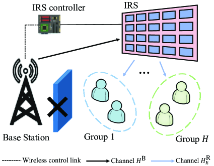
Figure 1: An IRS-aided mmWave multigroup multicast MIMO communication system.

We consider an IRS-aided mmWave multigroup multicast MIMO communication system in which a BS is equipped with $N^{\textrm{B}}$ antennas serving $K$ users via an IRS, as shown in Fig. 1. The users are divided into $H$ groups. We assume that the users in a group will request the same data streams and the data streams requested by the users in different groups are different. The set of user groups is denoted by $\mathcal{H}=\left\{1,2,\ldots,H\right\}$. Meanwhile, the set of users in a group $h$ is denoted as $\mathcal{H}_{h}$. We also assume that each user can only belong to one group, i.e., $\mathcal{H}_{i}\cap\mathcal{H}_{j}=\emptyset$, $\forall i,j\in\mathcal{H},i\neq j$. In our model, the direct communication link between the BS and a user is blocked due to unfavorable propagation conditions. Each user is equipped with $N^{\textrm{U}}$ antennas and $M^{\textrm{U}}$ RF chains to receive $\zeta$ data streams from the BS. The BS simultaneously transmits $H\zeta$ independent data streams to the users by $M^{\textrm{B}}$ RF chains. The main notations used in this work are summarized in Table I.

At the BS, the transmitted data streams of $H$ user groups are precoded by a baseband transmit beamforming matrix $\bm{F}^{\textrm{B}}=\left[\bm{F}^{\textrm{B}}_{1},\bm{F}^{\textrm{B}}_{2},\ldots,\bm{F}^{\textrm{B}}_{H}\right]\in\mathbb{C}^{M^{\textrm{B}}\times H\zeta}$, with $\bm{F}^{\textrm{B}}_{h}$ being the transmit beamforming matrix of group $h$. After that, each transmitted data stream of $H$ user groups is precoded by an RF transmit beamforming matrix $\bm{F}^{\textrm{R}}\in\mathbb{C}^{N^{\textrm{B}}\times M^{\textrm{B}}}$.

The received data streams of user $k$ in group $h$ are first processed by an RF receive beamforming matrix $\bm{W}_{k}^{\textrm{R}}\in\mathbb{C}^{N^{\textrm{U}}\times M^{\textrm{U}}}$. Then, user $k$ uses a baseband receive beamfoming matrix $\bm{W}_{k}^{\textrm{B}}\in\mathbb{C}^{M^{\textrm{U}}\times\zeta}$ to recover $\zeta$ data streams.

In our model, an IRS is used to enhance the received signal strength of users by reflecting signals from the BS to the users. We assume that the signal power of the multi-reflections (i.e., reflections more than once) on the IRS is ignored due to severe path loss. The phase-shift matrix of the IRS is $\bm{\Phi}=\text{diag}\left({e^{j{\phi_{1}}}},\ldots,{e^{j{\phi_{M}}}}\right)\in\mathbb{C}^{M\times M}$, where $\text{diag}\left({e^{j{\phi_{1}}}},\ldots,{e^{j{\phi_{M}}}}\right)$ is a diagonal matrix of $\left[{e^{j{\phi_{1}}}},\ldots,{e^{j{\phi_{M}}}}\right]$, $M$ is the number of reflecting elements at the IRS, and ${\phi_{m}}\in\left[0,2\pi\right]$ is the phase shift introduced by element $m$ of the IRS.

II-A1 Channel Model

The BS and the users employ uniform linear arrays (ULAs), and the IRS uses a uniform planar array (UPA). The normalized array response vector for an ULA is

$$\bm{a}\left(r\right)=\frac{1}{{\sqrt{N}}}{\left[1,\cdots,{e^{j\frac{{2\pi d}}{\lambda}\left(n-1\right)\sin\left(r\right)}},\cdots,{e^{j\frac{{2\pi d}}{\lambda}\left(N-1\right)\sin\left(r\right)}}\right]^{\textrm{T}}},$$ (1)

where $N$ is the number of antennas in ULA, $d$ is an interval between two antennas, and $\lambda$ is the signal wavelength. The normalized array response vector of UPA is

$$\begin{split}\bm{a}\left(\theta,\eta\right)=&\frac{1}{{\sqrt{{F_{y}}\times{F_{z}}}}}[1,\cdots,{e^{j\frac{{2\pi d}}{\lambda}\left(\left({f_{1}}-1\right)\cos\left(\eta\right)\sin\left(\theta\right)+\left({f_{2}}-1\right)\sin\left(\eta\right)\right)}},\\ &{\rm{}}\cdots,{e^{j\frac{{2\pi d}}{\lambda}\left(\left({F_{y}}-1\right)\cos\left(\eta\right)\sin\left(\theta\right)+\left({F_{z}}-1\right)\sin\left(\eta\right)\right)}}]^{\textrm{T}},\end{split}$$ (2)

where ${F_{y}}\times{F_{z}}$ is the number of elements in UPA, $F_{y}$ and $F_{z}$ are respectively the number of elements in the horizontal and vertical directions. The BS-IRS channel $\bm{H}^{\textrm{B}}\in\mathbb{C}^{M\times N^{\textrm{B}}}$ and the channel $\bm{H}^{\textrm{R}}_{k}\in\mathbb{C}^{N^{\textrm{U}}\times M}$ from the IRS to user $k$ in group $h$ can be respectively given as

$$\bm{H}^{\textrm{B}}=\sqrt{\frac{{{N^{\textrm{B}}}M}}{Y}}\sum\limits_{i=1}^{Y}{\alpha_{i}}\bm{a}\left(\theta_{i}^{\textrm{A}},\eta_{i}^{\textrm{A}}\right)\left(\bm{a}\left(r_{i}^{\textrm{D}}\right)\right)^{\textrm{H}},$$ (3)

$$\bm{H}^{\textrm{R}}_{k}=\sqrt{\frac{{M{N^{\textrm{U}}}}}{L}}\sum\limits_{i=1}^{L}{\beta_{i}}\bm{a}\left(r_{i,k}^{\textrm{A}}\right)\left(\bm{a}\left(\theta_{i}^{\textrm{D}},\eta_{i}^{\textrm{D}}\right)\right)^{{\textrm{H}}},$$ (4)

where $Y$ is the total number of paths (line-of-sight (LOS) and non-line-of-sight (NLOS)) between the BS and the IRS, $L$ is the total number of paths (LOS and NLOS) between the IRS and user $k$, $\theta_{i}^{\textrm{A}}$ denotes the azimuth angle of arrival of the IRS, $\theta_{i}^{\textrm{D}}$ denotes the azimuth angle of departure of the IRS, $\eta_{i}^{\textrm{A}}$ denotes the elevation angle of arrival of the IRS, $\eta_{i}^{\textrm{D}}$ denotes the elevation angle of departure of the IRS, $r_{i,k}^{\textrm{A}}$ represents the arrival angle of user $k$, $r_{i}^{\textrm{D}}$ represents the departure angle of the BS, ${\alpha_{i}}$ and ${\beta_{i}}$ are complex channel gains. ${\bm{a}}\left(r_{i}^{\textrm{D}}\right)$ and $\bm{a}\left(r_{i,k}^{\textrm{A}}\right)$ denote the normalized array response vectors of the BS and user $k$, respectively. $\left(\bm{a}\left(r_{i}^{\textrm{D}}\right)\right)^{\textrm{H}}$ is the Hermitian transpose of ${\bm{a}}\left(r_{i}^{\textrm{D}}\right)$. $\bm{a}\left(\theta_{i}^{\textrm{A}},\eta_{i}^{\textrm{A}}\right)$ represents the normalized array response vector of the IRS over the effective channel from the BS to the IRS. $\bm{a}\left(\theta_{i}^{\textrm{D}},\eta_{i}^{\textrm{D}}\right)$ represents the normalized array response vector of the IRS over the effective channel from the IRS to user $k$. The effective channel from the BS to user $k$ in group $h$ is ${\bm{H}}_{k}={G_{\textrm{t}}}{G_{\textrm{r}}}\bm{H}^{\textrm{R}}_{k}\bm{\Phi}\bm{H}^{\textrm{B}}$, where ${G_{\textrm{t}}}$ and ${G_{\textrm{r}}}$ are the antenna gains of the BS and each user, respectively.

II-A2 Data Rate Model

We assume that the BS obtains the channel state information (CSI). The BS is responsible for designing the reflection coefficients of the IRS. As a result, the detected data of user $k$ in group $h$ is given by

$$\hat{\bm{s}}_{k,h}\!=\!\left(\bm{W}_{k}^{\textrm{B}}\right)^{\textrm{H}}\left(\bm{W}_{k}^{\textrm{R}}\right)^{\textrm{H}}\bm{H}_{k}\bm{F}^{\textrm{R}}\bm{F}^{\textrm{B}}\bm{s}+\left(\bm{W}_{k}^{\textrm{B}}\right)^{\textrm{H}}\left(\bm{W}_{k}^{\textrm{R}}\right)^{\textrm{H}}\bm{n}_{k},$$ (5)

where $\bm{s}=\left[\bm{s}_{1}^{\textrm{T}},\ldots,\bm{s}_{H}^{\textrm{T}}\right]^{\textrm{T}}\in\mathbb{C}^{H\zeta\times 1}$ represents the data streams to be transmitted to all users, with $\bm{s}_{h}=\left[s_{h,1},\ldots,s_{h,\zeta}\right]^{\textrm{T}}\in\mathbb{C}^{\zeta\times 1}$ being $\zeta$ streams that will be transmitted to each user in group $h$. $\bm{n}_{k}\in\mathbb{C}^{N^{\textrm{U}}\times 1}$ is an additive white Gaussian noise vector of user $k$. Each element of $\bm{n}_{k}$ follows the independent and identically distributed complex Gaussian distribution with zero mean and variance $\sigma^{2}$. In (5), the first term represents the signal received by user $k$. The second term is the noise received by user $k$. The estimated data stream $i$ received by user $k$ in group $h$ can be expressed as

$$\begin{split}\hat{s}_{ik,h}&=\left(\bm{w}_{k,i}^{\textrm{B}}\right)^{\textrm{H}}\left(\bm{W}_{k}^{\textrm{R}}\right)^{\textrm{H}}\bm{H}_{k}\bm{F}^{\textrm{R}}\bar{\bm{f}}_{h_{i}}^{\textrm{B}}s_{h,i}\\ &+\sum_{j=1,j\neq i}^{\zeta}\left(\bm{w}_{k,i}^{\textrm{B}}\right)^{\textrm{H}}\left(\bm{W}_{k}^{\textrm{R}}\right)^{\textrm{H}}\bm{H}_{k}\bm{F}^{\textrm{R}}\bar{\bm{f}}_{h_{j}}^{\textrm{B}}s_{h,i}\\ &+\sum_{m=1,m\notin{\mathcal{H}_{h}}}^{H}\sum_{l=1}^{\zeta}\left(\bm{w}_{k,i}^{\textrm{B}}\right)^{\textrm{H}}\left(\bm{W}_{k}^{\textrm{R}}\right)^{\textrm{H}}\bm{H}_{k}\bm{F}^{\textrm{R}}\bar{\bm{f}}_{m_{l}}^{\textrm{B}}s_{m,l}\\ &+\left(\bm{w}_{k,i}^{\textrm{B}}\right)^{\textrm{H}}\left(\bm{W}_{k}^{\textrm{R}}\right)^{\textrm{H}}\bm{n}_{k},\end{split}$$ (6)

where $h_{i}=\left(h-1\right)\zeta+i$, $\bm{w}_{k,i}^{\textrm{B}}$ denotes row $i$ of matrix $\bm{W}_{k}^{\textrm{B}}$, and $\bar{\bm{f}}_{h_{i}}^{\textrm{B}}$ denotes column $h_{i}$ of matrix $\bm{F}^{\textrm{B}}$. In (6), the first term represents the desired signal. The second term is the interference caused by other streams of user $k$. The third term is the interference caused by the users from other groups. The fourth term is the noise. The SINR of user $k$ in group $h$ receiving data stream $i$ is given by

$$\begin{split}{{\xi_{ik,h}\left(\bm{W}_{k}^{\textrm{R}},\bm{W}_{k}^{\textrm{B}},{\bm{\nu}},\bm{F}^{\textrm{R}},\bm{F}^{\textrm{B}}_{h}\right)}}&=\\ &\!\!\!\!\!\!\!\!\!\!\!\!\!\!\frac{\left|\left(\bm{w}_{k,i}^{\textrm{B}}\right)^{\textrm{H}}\left(\bm{W}_{k}^{\textrm{R}}\right)^{\textrm{H}}\bm{H}_{k}\bm{F}^{\textrm{R}}\bar{\bm{f}}_{h_{i}}^{\textrm{B}}\right|^{2}}{{I_{ik,h}}+{J_{ik,h}}+\sigma^{2}},\end{split}$$ (7)

where ${I_{ik,h}}$ is short for ${I_{ik,h}}\left(\bm{W}_{k}^{\textrm{R}},\bm{W}_{k}^{\textrm{B}},{\bm{\nu}},\bm{F}^{\textrm{R}},\bm{F}^{\textrm{B}}_{h}\right)$ and ${I_{ik,h}}=\sum_{j=1,j\neq i}^{\zeta}\left|\left(\bm{w}_{k,i}^{\textrm{B}}\right)^{\textrm{H}}\left(\bm{W}_{k}^{\textrm{R}}\right)^{\textrm{H}}\bm{H}_{k}\bm{F}^{\textrm{R}}\bar{\bm{f}}_{h_{j}}^{\textrm{B}}\right|^{2}$ represents the interference from user itself, ${J_{ik,h}}$ is short for ${J_{ik,h}}\left(\bm{W}_{k}^{\textrm{R}},\bm{W}_{k}^{\textrm{B}},{\bm{\nu}},\bm{F}^{\textrm{R}},\bm{F}^{\textrm{B}}_{h}\right)$ and $J_{ik,h}=\sum_{m=1,m\notin{\mathcal{H}_{h}}}^{H}\sum_{l=1}^{\zeta}\left|\left(\bm{w}_{k,i}^{\textrm{B}}\right)^{\textrm{H}}\left(\bm{W}_{k}^{\textrm{R}}\right)^{\textrm{H}}\bm{H}_{k}\bm{F}^{\textrm{R}}\bar{\bm{f}}_{m_{l}}^{\textrm{B}}\right|^{2}$ represents the interference from other groups. The achievable data rate of user $k$ in group $h$ is given by

$$\begin{split}&{R_{k,h}}\left(\bm{W}_{k}^{\textrm{R}},\bm{W}_{k}^{\textrm{B}},{\bm{\nu}},\bm{F}^{\textrm{R}},\bm{F}^{\textrm{B}}_{h}\right)=\\ &\;\;\;\;\;\;\;\;\;\;\,W\sum_{i=1}^{\zeta}\log_{2}\left(1+{\xi_{ik,h}\left(\bm{W}_{k}^{\textrm{R}},\bm{W}_{k}^{\textrm{B}},{\bm{\nu}},\bm{F}^{\textrm{R}},\bm{F}^{\textrm{B}}_{h}\right)}\right),\end{split}$$ (8)

where $W$ is the bandwidth.

Due to the nature of the multicast mechanism, the achievable data rate of group $h$ depends on the user with minimum data rate, which is defined as follows:

$$\mathop{\min}\limits_{k\in{\mathcal{H}_{h}}}\left\{{R_{k,h}}\left(\bm{W}_{k}^{\textrm{R}},\bm{W}_{k}^{\textrm{B}},{\bm{\nu}},\bm{F}^{\textrm{R}},\bm{F}^{\textrm{B}}_{h}\right)\right\}.$$ (9)

II-B Problem Formulation

Next, we introduce our optimziation problem. Our goal is to maximize the sum rate of all the multicasting groups via jointly optimizing the transmit beamforming matrices $\bm{F}^{\textrm{B}}$, $\bm{F}^{\textrm{R}}$, the receive beamforming matrices $\bm{W}^{\textrm{R}}$, $\bm{W}^{\textrm{B}}$, and the phase shift ${\bm{\nu}}$ of the IRS. Mathematically, the optimization problem is formulated as

$$\mathop{\max}_{\bm{W}_{k}^{\textrm{B}},\bm{W}_{k}^{\textrm{R}},\bm{F}^{\textrm{R}},\bm{F}^{\textrm{B}},{\bm{\nu}}}\sum\limits_{h=1}^{H}{\mathop{\min}\limits_{k\in{\mathcal{H}_{h}}}\!\!\left\{{{R_{k,h}}\left(\bm{W}_{k}^{\textrm{R}},\bm{W}_{k}^{\textrm{B}},{\bm{\nu}},\bm{F}^{\textrm{R}},\bm{F}^{\textrm{B}}_{h}\right)}\right\}}$$ (10)

$$\textrm{s.t.}\ \ \left\|\bm{F}^{\textrm{R}}\bm{F}^{\textrm{B}}\right\|_{F}^{2}\leq P,$$ (10a)

$$\quad\>\ \ {\rm{}}\left|\bm{F}^{\textrm{R}}\left(i,j\right)\right|=\left|\bm{W}_{k}^{\textrm{R}}\left(i,j\right)\right|=1,\forall i,j,$$ (10b)

$$\quad\ \ \ 0\leq\phi_{m}\leq 2\pi,m=1,\ldots,M,$$ (10c)

where $P$ is the transmit power of the BS, $\left\|\bm{F}^{\textrm{R}}\bm{F}^{\textrm{B}}\right\|_{F}$ is the Frobenius norm of $\bm{F}^{\textrm{R}}\bm{F}^{\textrm{B}}$, $\bm{\nu}={\left[{e^{j{\phi_{1}}}},\ldots,{e^{j{\phi_{M}}}}\right]^{\textrm{H}}}$, $\bm{F}^{\textrm{R}}\left(i,j\right)$ denotes the element $\left(i,j\right)$ of matrix $\bm{F}^{\textrm{R}}$, with $\left|\bm{F}^{\textrm{R}}\left(i,j\right)\right|$ being the amplitude of $\bm{F}^{\textrm{R}}\left(i,j\right)$. The transmit power constraint of the BS is given in (10a). Constraint (10b) represents the amplitude constraints of the RF beamforming matrices of the BS and each user, while (10c) shows the phase shift limits of the IRS. Due to non-convex objective function (10) and non-convex constraints (10a)-(10c), problem (10) is non-convex, and hence it is hard to solve. Next, we introduce an efficient scheme to solve problem (10).

III Proposed Scheme

In this section, we first use the phase shift ${\bm{\nu}}$ of the IRS to represent the fully digital transmit beamforming matrix of the BS and receive beamforming matrix of the users. Then, we substitute them in (10) to transform problem (10). To solve the transformed problem, the phase shift ${\bm{\nu}}$ of the IRS is optimized by a manifold method. Finally, we introduce the entire algorithm used to solve problem (10).

III-A Block Diagonalization Method

III-A1 Simplification of Optimization Problem

$\bm{W}_{k}^{\textrm{B}}\bm{W}_{k}^{\textrm{R}}$ and $\bm{F}^{\textrm{R}}\bm{F}^{\textrm{B}}$ are regarded as a whole, that is, problem (10) is solved as a problem of fully digital beamforming. Once the fully digital transmit beamforming matrix and receive beamforming matrix are obtained, we can use the algorithm in [31] to find the hybrid transmit beamforming matrices and receive beamforming matrices to approximate the fully digital transmit beamforming matrix and receive beamforming matrix, as done in [32, 33]. Let $\bm{B}=\left[\bm{B}_{1},\ldots,\bm{B}_{H}\right]\in\mathbb{C}^{N^{\textrm{B}}\times H\zeta}$ be a fully digital transmit beamforming matrix which has the same size as the hybrid transmit beamforming matrix $\bm{F}^{\textrm{R}}\bm{F}^{\textrm{B}}$ and $\bm{J}_{k}\in\mathbb{C}^{N^{\textrm{U}}\times\zeta}$ be a fully digital receive beamforming matrix of user $k$ in group $h$. The size of $\bm{J}_{k}$ is equal to that of the hybrid receive beamforming matrix $\bm{W}_{k}^{\textrm{R}}\bm{W}_{k}^{\textrm{B}}$. Substituting $\bm{B}$ and $\bm{J}_{k}$ in (10), problem (10) can be transformed as

$$\mathop{\max}_{\bm{B},\bm{J},{\bm{\nu}}} \quad\sum\limits_{h=1}^{H}{\mathop{\min}\limits_{k\in{\mathcal{H}_{h}}}\left\{{{R_{k,h}}\left({{\bm{B}}_{h},{\bm{J}}_{k},{\bm{\nu}}}\right)}\right\}}$$ (11)

s.t. $$\left(\ref{PF1}\textrm{c}\right),$$

$$\,\left\|\bm{B}\right\|_{\textrm{F}}^{2}\leq P,$$ (11a)

where $\bm{J}=\text{diag}\left(\bm{J}_{1},\ldots,\bm{J}_{K}\right)$.

III-A2 Optimization of $\bm{B}$ and $\bm{J}$

Due to the low complexity of a BD method, we use it to find the relationship between ${\bm{\nu}}$ and the fully digital transmit beamforming matrix ${\bm{B}}$ of the BS as well as the receive beamforming matrix ${\bm{J}}$ of the users.

Lemma 1

Given ${\bm{\nu}}$ and the power allocation matrix ${{\bm{G}}_{h}}=\text{diag}\left(p_{1},\ldots,p_{\zeta}\right)$ in group $h$, where $p_{i}={{\frac{P}{{H\zeta}}}}$ is the transmit power of data stream $i$, $\bm{B}$ and $\bm{J}$ can be given by

$${\bm{B}}_{h}\left({\bm{\nu}}\right)=\tilde{\bm{V}}_{h}^{\left(0\right)}\left(\frac{{\bm{V}}_{1}^{\left(1\right)}+\cdots+{\bm{V}}_{K}^{\left(1\right)}}{\sqrt{\left|\mathcal{H}_{h}\right|}}\right){\sqrt{\frac{P}{{H\zeta}}}},$$ (12)

$${\bm{J}}_{k}\left({\bm{\nu}}\right)={\bm{U}}_{k}^{\left(1\right)},$$ (13)

where $\tilde{\bm{V}}_{h}^{\left(0\right)}=\text{null}\left(\tilde{\bm{H}}_{h}\right)$, ${\bm{U}}_{k}^{\left(1\right)}$, and ${{\bm{V}}_{k}^{\left(1\right)}}$ can be obtained by singular value decomposition (SVD) of ${\bm{H}}_{k}\tilde{\bm{V}}_{h}^{\left(0\right)}$ with ${\bm{H}}_{k}\tilde{\bm{V}}_{h}^{\left(0\right)}=\left[{\bm{U}}_{k}^{\left(1\right)},{\bm{U}}_{k}^{\left(2\right)}\right]\left[\begin{matrix}{\bm{\Sigma}}_{k}^{\left(1\right)}&\bm{0}&\\ \bm{0}&{\bm{\Sigma}}_{k}^{\left(2\right)}&\end{matrix}\!\!\!\!\!\right]\left[{\bm{V}}_{k}^{\left(1\right)},{\bm{V}}_{k}^{\left(2\right)}\right]^{\textrm{H}}$.

Proof:

To prove Lemma 1, we first define $\tilde{\bm{H}}_{h}$ as

$$\tilde{\bm{H}}_{h}\buildrel\Delta\over{=}\left[{\bm{H}}_{1},\ldots,{\bm{H}}_{h-1},{\bm{H}}_{h+1},\ldots,{\bm{H}}_{H}\right]^{\textrm{T}},$$ (14)

where $\bm{H}_{h-1}$ is the effective channels of all users in group $h-1$. We assume that the rank of $\tilde{\bm{H}}_{h}$ is $\tilde{L}_{k}$. Next, we introduce the use of BD method to represent the transmit beamforming matrices of the BS and the receive beamforming matrices of the users by the phase shifts of the IRS. To eliminate the inter-group interference, we define $\tilde{\bm{V}}_{h}^{\left(0\right)}\in\mathbb{C}^{N^{\textrm{B}}\times\left({N^{\textrm{B}}-\tilde{L}_{k}}\right)}$ as

$$\tilde{\bm{V}}_{h}^{\left(0\right)}=\text{null}\left(\tilde{\bm{H}}_{h}\right),$$ (15)

where $\text{null}\left(\tilde{\bm{H}}_{h}\right)$ represents that $\tilde{\bm{V}}_{h}^{\left(0\right)}$ lies in the null space of $\tilde{\bm{H}}_{h}$. Hence, we have $\tilde{\bm{H}}_{h}\tilde{\bm{V}}_{h}^{\left(0\right)}=\bm{0}$. The self interference of each user can be eliminated by the SVD of ${\bm{H}}_{k}\tilde{\bm{V}}_{h}^{\left(0\right)}$, which is

$${\bm{H}}_{k}\tilde{\bm{V}}_{h}^{\left(0\right)}=\left[{\bm{U}}_{k}^{\left(1\right)},{\bm{U}}_{k}^{\left(2\right)}\right]\left[\begin{matrix}{\bm{\Sigma}}_{k}^{\left(1\right)}&\bm{0}&\\ \bm{0}&{\bm{\Sigma}}_{k}^{\left(2\right)}&\end{matrix}\!\!\!\!\!\right]\left[{\bm{V}}_{k}^{\left(1\right)},{\bm{V}}_{k}^{\left(2\right)}\right]^{\textrm{H}}.$$ (16)

We assume that the rank of ${\bm{H}}_{k}\tilde{\bm{V}}_{h}^{\left(0\right)}$ is ${L}_{k}$, the column vectors of $\bm{U}_{k}^{\left(1\right)}\in\mathbb{C}^{N^{\textrm{U}}\times\zeta}$, $\bm{U}_{k}^{\left(2\right)}\in\mathbb{C}^{N^{\textrm{U}}\times\left({{L}_{k}-\zeta}\right)}$, $\bm{V}_{k}^{\left(1\right)}\in\mathbb{C}^{\left({N^{\textrm{B}}-\tilde{L}_{k}}\right)\times\zeta}$, and $\bm{V}_{k}^{\left(2\right)}\in\mathbb{C}^{\left({N^{\textrm{B}}-\tilde{L}_{k}}\right)\times\left({{L}_{k}-\zeta}\right)}$ can form orthonormal sets, ${\bm{\Sigma}}_{k}^{\left(1\right)}\in\mathbb{C}^{\zeta\times\zeta}$ and ${\bm{\Sigma}}_{k}^{\left(2\right)}\in\mathbb{C}^{\left({{L}_{k}-\zeta}\right)\times\left({{L}_{k}-\zeta}\right)}$ are diagonal matrices of singular values. ${\bm{B}}_{h}\left({\bm{\nu}}\right)$ must be designed to cancel the inter-group interference as well as the interference of all users in this group. Thus, $\tilde{\bm{V}}_{h}^{\left(0\right)}$ and $\sum\limits_{i=1}^{K}{\bm{V}_{i}^{\left(1\right)}}$ must be included in ${\bm{B}}_{h}\left({\bm{\nu}}\right)$, which can be given by

$${\bm{B}}_{h}\left({\bm{\nu}}\right)=\tilde{\bm{V}}_{h}^{\left(0\right)}\left(\frac{{\bm{V}}_{1}^{\left(1\right)}+\cdots+{\bm{V}}_{K}^{\left(1\right)}}{\sqrt{\left|\mathcal{H}_{h}\right|}}\right){{\bm{G}}_{h}^{1/2}},$$ (17)

where $\left|\mathcal{H}_{h}\right|$ is the number of users in group $h$, $\frac{1}{\sqrt{\left|\mathcal{H}_{h}\right|}}$ ensures that the power of $\left(\frac{{\bm{V}}_{1}^{\left(1\right)}+\cdots+{\bm{V}}_{K}^{\left(1\right)}}{\sqrt{\left|\mathcal{H}_{h}\right|}}\right)$ is unit, and ${{\bm{G}}_{h}}$ is the power allocation matrix in group $h$. To eliminate the interference of all users in this group, the fully digital receive beamforming matrix ${\bm{J}}_{k}$ of user $k$ in group $h$ is written as

$$\begin{split}{\bm{J}}_{k}\left({\bm{\nu}}\right)&={\bm{U}}_{k}^{\left(1\right)}.\end{split}$$ (18)

Substituting ${{\bm{G}}_{h}}$ into (17), we have

$${\bm{B}}_{h}\left({\bm{\nu}}\right)=\tilde{\bm{V}}_{h}^{\left(0\right)}\left(\frac{{\bm{V}}_{1}^{\left(1\right)}+\cdots+{\bm{V}}_{K}^{\left(1\right)}}{\sqrt{\left|\mathcal{H}_{h}\right|}}\right){\sqrt{\frac{P}{{H\zeta}}}}.$$ (19)

This completes the proof. ∎

From Lemma 1, we can see that ${\bm{B}}_{h}\left({\bm{\nu}}\right)$ mainly depends on the orthogonal bases of the null space of users in other groups, the orthogonal bases of the subspace of users in group $h$, the maximum transmit power of the BS and number of groups, ${\bm{J}}_{k}\left({\bm{\nu}}\right)$ depends on the effective channel of user $k$ and the orthogonal bases of the null space of users in other groups.

III-A3 Simplification of Problem (11)

Based on the Lemma 1, the interference caused by other groups ${J_{ik,h}}$ and user itself ${I_{ik,h}}$ can be eliminated by the fully digital transmit beamforming matrix ${\bm{B}}_{h}\left({\bm{\nu}}\right)$ and receive beamforming matrix ${\bm{J}}_{k}\left({\bm{\nu}}\right)$. Substituting ${\bm{B}}_{h}\left({\bm{\nu}}\right)$ and ${\bm{J}}_{k}\left({\bm{\nu}}\right)$ into (11), the achievable data rate of user $k$ in group $h$ can be rewritten as follows:

$$\begin{split}&{R_{k,h}}\left({{\bm{B}}_{h}\left({\bm{\nu}}\right),{\bm{J}}_{k}\left({\bm{\nu}}\right),{\bm{\nu}}}\right)=\\ &\;\;\;\;\;\;W\sum_{i=1}^{\zeta}\log_{2}\left(1+{\left|\left(\bm{j}_{k,i}\left({\bm{\nu}}\right)\right)^{\textrm{H}}\bm{H}_{k}\bar{\bm{b}}_{h,i}\left({\bm{\nu}}\right)\right|^{2}}/{\sigma^{2}}\right),\\ \end{split}$$ (20)

Let $\frac{\left|\left(\bm{j}_{k,i}\left({\bm{\nu}}\right)\right)^{\textrm{H}}\bm{H}_{k}\bar{\bm{b}}_{h,i}\left({\bm{\nu}}\right)\right|^{2}}{\sigma^{2}}={\lambda_{i}}$, (20) can be rewritten by

$$\begin{split}&{R_{k,h}}\left({{\bm{B}}_{h}\left({\bm{\nu}}\right),{\bm{J}}_{k}\left({\bm{\nu}}\right),{\bm{\nu}}}\right)\\ &=W\sum_{i=1}^{\zeta}\log_{2}\left(1+{\lambda_{i}}\right),\\ &=W\log_{2}\left(1+{\lambda_{1}}\right)+\ldots+\log_{2}\left(1+{\lambda_{\zeta}}\right),\\ &=W\log_{2}\left(\left(1+{\lambda_{1}}\right)*\ldots*\left(1+{\lambda_{\zeta}}\right)\right),\\ &=W\log_{2}\left|\begin{matrix}1+{\lambda_{1}}&\cdots&0&\\ \vdots&\ddots&\vdots&\\ 0&\cdots&1+{\lambda_{\zeta}}\end{matrix}\!\!\!\!\!\right|.\end{split}$$ (21)

Therefore, we have

$$\begin{split}&{R_{k,h}}\left({{\bm{B}}_{h}\left({\bm{\nu}}\right),{\bm{J}}_{k}\left({\bm{\nu}}\right),{\bm{\nu}}}\right)\\ &=W\log_{2}\text{det}\left(\bm{I}_{\zeta}+{\left|\left({\bm{J}}_{k}\left({\bm{\nu}}\right)\right)^{\textrm{H}}\bm{H}_{k}\bm{B}_{h}\left({\bm{\nu}}\right)\right|^{2}}/{\sigma^{2}}\right),\end{split}$$ (22)

where $\text{det}(\cdot)$ represents the determinant of a square matrix, and $\bm{I}_{\zeta}$ is an $\zeta\times\zeta$ identity matrix. Substituting ${\bm{B}}_{h}\left({\bm{\nu}}\right)$ and ${\bm{J}}_{k}\left({\bm{\nu}}\right)$ into (22), we have

$$\begin{split}&{R_{k,h}}\left({{\bm{B}}_{h}\left({\bm{\nu}}\right),{\bm{J}}_{k}\left({\bm{\nu}}\right),{\bm{\nu}}}\right)\\ &=W\log_{2}\text{det}\!\left(\!\bm{I}_{\zeta}\!+\!\frac{\left|\!\left(\!{\bm{U}}_{k}^{\left(1\right)}\right)^{\textrm{H}}\!\!\bm{H}_{k}\!\tilde{\bm{V}}_{h}^{\left(0\right)}\!\!\left(\!\frac{\sum\limits_{i=1}^{K}{\bm{V}_{i}^{\left(1\right)}}}{\sqrt{\left|\mathcal{H}_{h}\right|}}\!\right)\!{\sqrt{\frac{P}{{H\zeta}}}}\right|^{2}}{\sigma^{2}}\right).\end{split}$$ (23)

Since ${\bm{H}}_{i}\left({\bm{H}}_{k}\right)^{\textrm{H}}=\bm{0}$ $\left(i\neq k\right)$, we have ${\bm{H}}_{k}\left({\bm{V}}_{i}^{\left(1\right)}\right)^{\textrm{H}}=\bm{0}$ $\left(i\neq k\right)$. Substituting (16) into (23), we have

$$\begin{split}&{R_{k,h}}\left({{\bm{B}}_{h}\left({\bm{\nu}}\right),{\bm{J}}_{k}\left({\bm{\nu}}\right),{\bm{\nu}}}\right)\\ &=W\log_{2}\text{det}\left(\bm{I}_{\zeta}+{\frac{P}{{\left|\mathcal{H}_{h}\right|}H\zeta\sigma^{2}}}\left({\bm{\Sigma}}_{k}^{\left(1\right)}\right)^{2}\right),\end{split}$$ (24)

Then, the optimization problem in (11) can be transformed as

$$\begin{split}\mathop{\max}\limits_{{\bm{\nu}}}&\sum\limits_{h=1}^{H}{\mathop{\min}\limits_{k\in{\mathcal{H}_{h}}}\left\{W{\log_{2}\text{det}\left(\bm{I}_{\zeta}+{\frac{P}{{\left|\mathcal{H}_{h}\right|}H\zeta\sigma^{2}}}\left({\bm{\Sigma}}_{k}^{\left(1\right)}\right)^{2}\right)}\right\}}\\ \textrm{s.t.}&\quad\left(\ref{PF1}\textrm{c}\right).\end{split}$$ (25)

III-B Phase Optimization with Manifold Method

III-B1 Approximation of ${\bm{\Sigma}}_{k}^{\left(1\right)}$

Since ${\bm{\Sigma}}_{k}^{\left(1\right)}$ in (25) is unknown, we use the function of phase shift to represent ${\bm{\Sigma}}_{k}^{\left(1\right)}$, which is proved in Theorem 1.

Theorem 1

${\bm{\Sigma}}_{k}^{\left(1\right)}\left(i,j\right)\approx{\beta_{i}}{\alpha_{j}}{\bm{\nu}}^{\textrm{H}}{{\bm{c}}^{ij}}$, where ${{\bm{c}}^{ij}}=\left(\bm{a}\left({\theta}_{i}^{{\textrm{D}}},{\eta}_{i}^{{\textrm{D}}}\right)\right)^{{\textrm{*}}}\circ\bm{a}\left({\theta}_{j}^{{\textrm{A}}},{\eta}_{j}^{{\textrm{A}}}\right)$ with $\left(\bm{a}\left({\theta}_{i}^{{\textrm{D}}},{\eta}_{i}^{{\textrm{D}}}\right)\right)^{{\textrm{*}}}$ being the conjugate of $\left(\bm{a}\left({\theta}_{i}^{{\textrm{D}}},{\eta}_{i}^{{\textrm{D}}}\right)\right)$ and $\circ$ being the Hadamard product.

Proof:

See Appendix A. ∎

From Theorem 1, we can see that ${\bm{\Sigma}}_{k}^{\left(1\right)}$ depends on the distance ${\alpha_{j}}$ between the BS and the IRS, the distance ${\beta_{i}}$ between the IRS and user $k$, the angle $\bm{a}\left({\theta}_{j}^{{\textrm{A}}},{\eta}_{j}^{{\textrm{A}}}\right)$ from the BS to the IRS, the phase shifts of the IRS, and the angle $\bm{a}\left({\theta}_{i}^{{\textrm{D}}},{\eta}_{i}^{{\textrm{D}}}\right)$ from the IRS to user $k$.

III-B2 Problem Transformation

Based on Theorem 1, the optimization problem (25) can be rewritten as

$$\mathop{\max}\limits_{\bm{\nu}}\sum\limits_{h=1}^{H} {\mathop{\min}\limits_{k\in{\mathcal{H}_{h}}}W\left\{\sum\limits_{i=1}^{\zeta}{\log_{2}\left(1+{\frac{P}{{\left|\mathcal{H}_{h}\right|}H\zeta\sigma^{2}}}\left|\bm{D}_{k}\left(i,i\right)\right|^{2}\right)}\right\}}$$ (26)

s.t. $$\!\!\left(\ref{PF1}\textrm{c}\right),$$

$${\left|{{d_{ij}}}\right|}=\left|{{\bm{\nu}}^{H}{{\bm{c}}^{ij}}}\right|\textless\tau,\quad\forall i\neq j,$$ (26a)

where ${d_{ii}}={\bm{\nu}}^{H}{{\bm{c}}^{ii}}$, $\bm{D}_{k}\left(i,i\right)={\alpha_{i}}{\beta_{i}}{d_{ii}}$ ($i\in\left\{1,\ldots,{\zeta}\right\}$), and $\tau$ is a small positive value. Constraint (26a) is to make sure that $\bm{D}_{k}$ is approximately a non-square diagonal matrix such that ${\bm{H}}_{k}\tilde{\bm{V}}_{h}^{\left(0\right)}=\bm{A}_{k}\bm{D}_{k}\left(\bm{A}\right)^{{\textrm{H}}}\left[\bm{z}_{\left(K-{\left|\mathcal{H}_{h}\right|}\right){\zeta}+1};\ldots;\bm{z}_{K{\zeta}}\right]$ can be treated as an approximation of the truncated SVD of ${\bm{H}}_{k}\tilde{\bm{V}}_{h}^{\left(0\right)}$, where $\bm{z}_{\left(K-{\left|\mathcal{H}_{h}\right|}\right){\zeta}+1}$ denotes row ${\left(K-{\left|\mathcal{H}_{h}\right|}\right){\zeta}+1}$ of matrix ${\bm{Z}}$. Constraint (26a) can be removed and this omission does not affect the validity of our proposed solution[15]. Hence, problem (26) can be rewritten as follows:

$$\begin{split}\mathop{\max}\limits_{\bm{\nu}}&\sum\limits_{h=1}^{H}{\mathop{\min}\limits_{k\in{\mathcal{H}_{h}}}W\left\{\sum\limits_{i=1}^{\zeta}{\log_{2}\left(1+{\frac{P}{{\left|\mathcal{H}_{h}\right|}H\zeta\sigma^{2}}}\left|\bm{D}_{k}\left(i,i\right)\right|^{2}\right)}\right\}}\\ \textrm{s.t.}&\quad\;\left(\ref{PF1}\textrm{c}\right).\end{split}$$ (27)

Substituting $\bm{D}_{k}\left(i,i\right)={\alpha_{i}}{\beta_{i}}{\bm{\nu}}^{H}{{\bm{c}}^{ii}}$ into (27), the problem (27) can be transformed as follows:

$$\vspace{-.3em}\begin{split}\mathop{\max}\limits_{\bm{\nu}}&\quad\sum\limits_{h=1}^{H}{\mathop{\min}\limits_{k\in{\mathcal{H}_{h}}}W\left\{\sum\limits_{i=1}^{\zeta}{\log_{2}\left(1+{b_{i}}{\bm{\nu}}^{\textrm{H}}{{\bm{C}}^{ii}}{\bm{\nu}}\right)}\right\}}\\ \textrm{s.t.}&\quad\;\left(\ref{PF1}\textrm{c}\right),\end{split}$$ (28)

where ${{\bm{C}}^{ii}}\buildrel\Delta\over{=}{{\bm{c}}^{ii}}\left({\bm{c}}^{ii}\right)^{\textrm{H}}$ and ${b_{i}}\buildrel\Delta\over{=}{\frac{P}{{\left|\mathcal{H}_{h}\right|}H\zeta\sigma^{2}}}\left|{\alpha_{i}}{\beta_{i}}\right|^{2}$.

III-B3 Solution of Problem (28)

Since constraint (10c) has a manifold structure, problem (28) can be regarded as a manifold-constrained optimization problem. Next, we introduce the use of a manifold method [34] to solve problem (28). In particular, we first introduce the definition of a tangent space. Then, similar to the gradient in Euclidean space, we introduce the gradient on the manifold, called the Riemannian gradient. Finally, problem (28) is solved by an iterative method using the Riemannian gradient.

To solve problem (28), we first rewrite the objective function as

$$\begin{split}f\left(\bm{\nu}\right)\buildrel\Delta\over{=}-\sum\limits_{h=1}^{H}{\mathop{\min}\limits_{k\in{\mathcal{H}_{h}}}W\left\{\sum\limits_{i=1}^{\zeta}{\log_{2}\left(1+{b_{i}}{\bm{\nu}}^{\textrm{H}}{{\bm{C}}^{ii}}{\bm{\nu}}\right)}\right\}}.\end{split}$$ (29)

Let ${{\bm{\nu}}_{n}}$ be the value at iteration $n$. Based on (29), the Euclidean gradient of the objective function $f\left(\bm{\nu}\right)$ at point ${{\bm{\nu}}_{n}}$ is given by

$$\begin{split}\nabla f\left({{\bm{\nu}}_{n}}\right)&=-\sum\limits_{h=1}^{H}{\mathop{\min}\limits_{k\in{\mathcal{H}_{h}}}\left\{\nabla\left({R_{k,h}}\left({{\bm{B}}_{h}\left({\bm{\nu}_{n}}\right),{\bm{J}}_{k}\left({\bm{\nu}_{n}}\right),{\bm{\nu}_{n}}}\right)\right)\right\}},\\ &=-\sum\limits_{h=1}^{H}{\mathop{\min}\limits_{k\in{\mathcal{H}_{h}}}W\left\{\sum\limits_{i=1}^{\zeta}\frac{1}{{\textrm{ln2}}}\frac{2{b_{i}}{{\bm{C}}^{ii}}{{\bm{\nu}}_{n}}}{1+{b_{i}}\left({\bm{\nu}}_{n}\right)^{\textrm{H}}{{\bm{C}}^{ii}}{{\bm{\nu}}_{n}}}\right\}}.\end{split}$$ (30)

To introduce the Riemannian gradient, we first define a tangent space of of an oblique manifold $\mathcal{Q}$ at point ${\bm{\nu}}_{n}$ as

$$\begin{split}{{{T}_{{\bm{\nu}}_{n}}}\mathcal{Q}}=\left\{{\bm{u}\in\mathbb{C}^{G}}|\left[\bm{u}{{\bm{\nu}}_{n}^{\textrm{H}}}\right]_{g,g}=0,\forall g\in\mathcal{G}=\left\{1,2,...,G\right\}\right\}.\end{split}$$ (31)

From (31), we see that the tangent space containts all the tangent vectors of $\mathcal{Q}$ at ${\bm{\nu}}_{n}$.

The Riemannian gradient of the objective function $f\left(\bm{\nu}\right)$ at point ${{\bm{\nu}}_{n}}$ can be obtained by orthogonally projecting the Euclidean gradient $\nabla f\left({{\bm{\nu}}_{n}}\right)$ onto the tangent space ${{{T}_{{\bm{\nu}}_{n}}}\mathcal{Q}}$, which is given by

$$\begin{split}{\mathcal{G}_{{\bm{\nu}}_{n}}\mathcal{Q}}&=\nabla f\left({{\bm{\nu}}_{n}}\right)-{\textrm{Real}}\left\{\nabla f\left({{\bm{\nu}}_{n}}\right)\circ{\left({\bm{\nu}}_{n}^{\textrm{T}}\right)^{\textrm{H}}}\right\}\circ{\bm{\nu}}_{n},\end{split}$$ (32)

where ${\textrm{Real}}(\bm{M})$ is the real part of $\bm{M}$ and ${\textrm{Real}}\left\{\nabla f\left({{\bm{\nu}}_{n}}\right)\circ{\left({\bm{\nu}}_{n}^{\textrm{T}}\right)^{\textrm{H}}}\right\}\circ{\bm{\nu}}_{n}$ is the projected gradient of Euclidean gradient $\nabla f\left({{\bm{\nu}}_{n}}\right)$ on the tangent space ${{{T}_{{\bm{\nu}}_{n}}}\mathcal{Q}}$.

Given the Riemannian gradient, we use the optimization method in Euclidean space to solve the manifold-constrained optimization problem[35]. The update of ${\bm{\nu}}_{n}$ is

$$\begin{split}\bar{\bm{\nu}}_{n}={\bm{\nu}}_{n}-{\tilde{\lambda}_{n}}{\mathcal{G}_{{\bm{\nu}}_{n}}\mathcal{Q}},\end{split}$$ (33)

where ${\tilde{\lambda}_{n}}$ is the step size. To ensure that the updated value of ${\bm{\nu}_{n}}$ lies in the feasible set, we have

$$\begin{split}{\bm{\nu}}_{n+1}=\bar{\bm{\nu}}_{n}\circ\frac{1}{\left|{\bar{\bm{\nu}}_{n}}\right|}.\end{split}$$ (34)

The detailed process of using the manifold-based method to solve problem (28) is given in Algorithm 1. Given ${\bm{\nu}}$, we can use Lemma 1 to calculate ${\bm{B}}_{h}\left({\bm{\nu}}\right)$ and ${\bm{J}}_{k}\left({\bm{\nu}}\right)$.

Algorithm 1 Proposed Design for Solving (28)

1:  Initialize ${\bm{\nu}}_{0}\in{\mathcal{Q}}$.

2:  Obtain ${d_{ij}}$ according to (45).

3:  Obtain ${{\bm{C}}^{ii}}$ and ${b_{i}}$ according to (28).

4:  repeat

5:     Compute the Euclidean gradient using (30).

6:     Compute the Riemannian gradient by (32).

7:     Update ${\bm{\nu}}_{n+1}$ by (34).

8:  until the objective function converges.

9:  ${\bm{\Phi}}=\text{diag}({\bm{\nu}}^{\textrm{H}})$.

III-C Optimization of the Transmit Beamforming Matrices of the BS and the Receive Beamforming Matrices of Users

Given ${\bm{B}}_{h}\left({\bm{\nu}}\right)$ and ${\bm{J}}_{k}\left({\bm{\nu}}\right)$, we next introduce the use of the algorithm in [31] to optimize ${\bm{F}^{\textrm{B}}}$, ${\bm{F}^{\textrm{R}}}$, $\bm{W}_{k}^{\textrm{B}}$, and $\bm{W}_{k}^{\textrm{R}}$.

Since we have assumed that $\bm{B}=\left[\bm{B}_{1},\ldots,\bm{B}_{H}\right]\in\mathbb{C}^{N^{\textrm{B}}\times H\zeta}$ is a fully digital transmit beamforming matrix which has the same size as the hybrid transmit beamforming matrix $\bm{F}^{\textrm{R}}\bm{F}^{\textrm{B}}$ and we have also replaced $\bm{F}^{\textrm{R}}\bm{F}^{\textrm{B}}$ with $\bm{B}$ in problem (11), the problem of optimizing ${\bm{F}^{\textrm{B}}}$ and ${\bm{F}^{\textrm{R}}}$ can be formulated as

$$\mathop{\min}_{\bm{F}^{\textrm{R}},\bm{F}^{\textrm{B}}}\left\|\bm{B}-\bm{F}^{\textrm{R}}\bm{F}^{\textrm{B}}\right\|_{F}^{2}$$ (35)

$$\quad\>\ \ {\rm{}}\left|\bm{F}^{\textrm{R}}\left(i,j\right)\right|=1,\forall i,j,$$ (35a)

Due to the unit modulus constraints of (35a), vector $\bm{x}=\textrm{v}\left(\bm{F}^{\textrm{R}}\right)$ forms a complex circle manifold $\left\{\bm{x}\in\mathbb{C}^{w}:{\rm{}}\left|\bm{x}_{1}\right|=\left|\bm{x}_{2}\right|=\cdots=\left|\bm{x}_{w}\right|=1\right\}$, where $\textrm{v}\left(\bm{F}^{\textrm{R}}\right)$ is the vectorization of $\bm{F}^{\textrm{R}}$ and $w=N^{\textrm{B}}M^{\textrm{B}}$. Hence, problem (35) can be transformed to an unconstrained optimization problem on manifolds. The iterative algorithm used to solve problem (28) can be used to solve it. In particular, $\bm{x}^{n}$ can be updated using (33) and (34). Given the updated $\bm{x}$ with $\bm{x}=\textrm{v}\left(\bm{F}^{\textrm{R}}\right)$, the update of the RF transmit beamforming matrix at iteration $n$ can be expressed as

$$\bm{F}^{\textrm{R}}_{n}=\textrm{v}^{-1}\left(\bm{x}^{n}\right),$$ (36)

where $\textrm{v}^{-1}\left(\bm{x}^{n}\right)$ is the inverse-vectorization of $\bm{x}^{n}$. Given $\bm{F}^{\textrm{R}}_{n}$, the optimization problem in (35) can be simplified as follows:

$$\mathop{\min}_{\bm{F}^{\textrm{B}}}\left\|\bm{B}-\bm{F}^{\textrm{R}}_{n}\bm{F}^{\textrm{B}}\right\|_{F}^{2}.$$ (37)

Since problem (37) is a least-square optimization problem, $\bm{F}^{\textrm{B}}$ at iteration $n$ can be given by

$$\bm{F}^{\textrm{B}}_{n}=\left(\bm{F}^{\textrm{R}}_{n}\right)^{\dagger}\bm{B},$$ (38)

where $\left(\bm{F}^{\textrm{R}}_{n}\right)^{\dagger}$ is the Moore-Penrose pseudo inverse of $\bm{F}^{\textrm{R}}_{n}$. At convergence, ${\bm{F}^{\textrm{R}}}$ is expressed as

$${\bm{F}^{\textrm{R}}}=\textrm{v}^{-1}\left(\bm{x}^{n+1}\right).$$ (39)

To satisfy constraint (10a), ${\bm{F}^{\textrm{B}}}$ is expressed as

$${\bm{F}^{\textrm{B}}}=\frac{\sqrt{P}}{\left\|\bm{F}^{\textrm{R}}\bm{F}^{\textrm{B}}_{n}\right\|_{F}}\bm{F}^{\textrm{B}}_{n}.$$ (40)

Similarly, given ${\bm{J}}_{k}\left({\bm{\nu}}\right)$, the problem of optimizing $\bm{W}_{k}^{\textrm{B}}$ and $\bm{W}_{k}^{\textrm{R}}$ can be given as follows:

$$\mathop{\min}_{\bm{W}_{k}^{\textrm{R}},\bm{W}_{k}^{\textrm{B}}}\left\|\bm{J}_{k}-\bm{W}_{k}^{\textrm{R}}\bm{W}_{k}^{\textrm{B}}\right\|_{F}^{2}$$ (41)

$$\quad\>\ \ \ {\rm{}}\left|\bm{W}_{k}^{\textrm{R}}\left(i,j\right)\right|=1,\forall i,j.$$ (41a)

Since this optimization problem is similar to the problem in (35), we can use the same method used to solve problem (35) to optimize $\bm{W}_{k}^{\textrm{B}}$ and $\bm{W}_{k}^{\textrm{R}}$.

III-D Complexity Analysis

The proposed algorithm for solving problem (10) is summarized in Algorithm 2. The complexity of Algorithm 2 lies in the calculation of (17), solving problem (28), and using the algorithm in [31] to find $\hat{\bm{F}^{\textrm{B}}},\hat{\bm{F}^{\textrm{R}}}$, $\hat{\bm{W}_{k}^{\textrm{B}}}$, and $\hat{\bm{W}_{k}^{\textrm{R}}}$.

The complexity of calculating (17) is $\mathcal{O}\left(\left(N^{\textrm{B}}\right)^{3}+{\left|\mathcal{H}_{h}\right|}\left(N^{\textrm{B}}\right)^{2}\zeta\right)$. The complexity of solving problem (28) lies in computing the Euclidean gradient of the objective function in (28) at each iteration, which involves the complexity of $\mathcal{O}\left(H{M}^{2}\zeta\right)$. Hence, the total complexity of solving problem (28) is $\mathcal{O}\left(H{M}^{2}\zeta{S_{1}}\right)$, where ${S_{1}}$ is the number of iterations of using the manifold method to solve problem (28). The complexity of using the algorithm in [31] to find $\hat{\bm{F}^{\textrm{B}}},\hat{\bm{F}^{\textrm{R}}}$, $\hat{\bm{W}_{k}^{\textrm{B}}}$, and $\hat{\bm{W}_{k}^{\textrm{R}}}$ is $\mathcal{O}\left(N^{\textrm{B}}M^{\textrm{B}}\zeta{S_{2}}+N^{\textrm{U}}M^{\textrm{U}}\zeta{S_{2}}\right)$, where ${S_{2}}$ is the number of iterations required to converge. Hence, the total complexity of solving problem (10) is $\mathcal{O}\left(\left(N^{\textrm{B}}\right)^{3}+{\left|\mathcal{H}_{h}\right|}\left(N^{\textrm{B}}\right)^{2}\zeta+H{M}^{2}\zeta{S_{1}}+N^{\textrm{B}}M^{\textrm{B}}\zeta{S_{2}}+N^{\textrm{U}}M^{\textrm{U}}\zeta{S_{2}}\right)\\ \approx O\left(\left(N^{\textrm{B}}\right)^{3}+H{M}^{2}\zeta{S_{1}}\right)$.

Algorithm 2 Proposed Scheme for Solving Problem (10)

1:  Input: $\bm{H}^{\textrm{B}},\bm{H}^{\textrm{R}}_{k},\zeta,P,\sigma^{2}$.

2:  Calculate ${\bm{B}}_{h}\left({\bm{\nu}}\right)$ and ${\bm{J}}_{k}\left({\bm{\nu}}\right)$ by Lemma 1.

3:  Find the phase shift $\hat{\bm{\nu}}$ of the IRS by solving problem (28).

4:  Obtain ${\bm{B}}_{h}\left(\hat{\bm{\nu}}\right)$ and ${\bm{J}}_{k}\left(\hat{\bm{\nu}}\right)$ by Lemma 1.

5:  Calculate $\hat{\bm{F}^{\textrm{B}}},\hat{\bm{F}^{\textrm{R}}},$ $\hat{\bm{W}_{k}^{\textrm{B}}}$, and $\hat{\bm{W}_{k}^{\textrm{R}}}$ by the algorithm in [31].

6:  Output: $\hat{\bm{\nu}},\hat{\bm{F}^{\textrm{B}}},\hat{\bm{F}^{\textrm{R}}}$, $\hat{\bm{W}_{k}^{\textrm{B}}}$, $\hat{\bm{W}_{k}^{\textrm{R}}}$.

III-E Convergence Analysis

Theorem 2

Assume that there exists $\bm{\nu}^{*}$ such that $\mathcal{G}_{\bm{\nu}^{*}}\mathcal{Q}=\bm{0}$. Then, there exists a neighborhood $\mathcal{U}$ of $\bm{\nu}^{*}$ in $\mathbb{C}^{G}$, such that for all $\bm{\nu}_{0}\in\mathcal{U}$, Algorithm 1 generates an infinite sequence $\{\bm{\nu}_{n}\}$ converging to $\bm{\nu}^{*}$.

Proof:

According to [34, Theorem 6.3.2], there exists $\gamma_{R}$ such that

$$\|\bm{\nu}_{n+1}-\bar{\bm{\nu}}_{n}\|\leq\gamma_{R}\|{\bm{\nu}}_{n}-{\bm{\nu}}^{*}\|^{2}.$$ (42)

Based on Algorithm 1, we further have

$$\|\bm{\nu}_{n+1}-{\bm{\nu}}^{*}\| \leq\|\bm{\nu}_{n+1}-\bar{\bm{\nu}}_{n}\|+\|\bar{\bm{\nu}}_{n}-{\bm{\nu}}^{*}\|$$

$$\leq\|{\bm{\nu}}_{n}-{\bm{\nu}}^{*}-\tilde{\lambda}_{n}\mathcal{G}_{\bm{\nu}^{*}}\mathcal{Q}\|$$

$$+\gamma_{R}\|{\bm{\nu}}_{n}-{\bm{\nu}}^{*}\|^{2}$$

$$=\gamma_{T}\|{\bm{\nu}}_{n}-{\bm{\nu}}^{*}\|^{2}+\gamma_{R}\|{\bm{\nu}}_{n}-{\bm{\nu}}^{*}\|^{2}$$ (43)

where the last inequality follows from the Lipschitz-continuous differential of function $f(\bm{\nu})$ and $\gamma_{T}>0$ is a parameter related to the step-size $\tilde{\lambda}_{n}$ [34, Theorem 6.3.2]. ∎

IV Simulation Results

In our simulations, the coordinates of the BS and the IRS are (2m, 0m, 10m) and (0m, 148m, 10m), respectively. All users are randomly distributed in a circle centered at (7m, 148m, 1.8m) with a radius being 10 m. The bandwidth is set to 251.1886 MHz. The values of other parameters are defined in Table II. For comparison purposes, we consider five baselines: a) the fully digital beamforming matrices of the BS and the users as well as the phase of each element of the IRS are optimized by the proposed scheme, which is the solution for problem (11), b) the hybrid beamforming matrices of the BS and the users are determined by the proposed algorithm and the phase shifts of the IRS are randomly determined, c) the fully digital beamforming matrices of the BS and the users are determined by the proposed scheme while the phase shifts of the IRS are randomly determined, d) the hybrid beamforming matrices of the BS and the users are determined by the algorithm in [15] and the phase of each element of the IRS are optimized by the proposed scheme, e) the fully digital beamforming matrices of the BS and the users are determined by the scheme in [15] as well as the phase of each element of the IRS are optimized by the proposed scheme.

TABLE II: Simulation Parameters

Parameters	Values	Parameters	Values
$M$	$16\times 16$	$N^{\textrm{B}}$	64
$N^{\textrm{U}}$	64	$M^{\textrm{B}}$	8
$M^{\textrm{U}}$	4	${\zeta}$	4
$Y=L$	7	${G_{\textrm{t}}}$	24.5 dBi
${G_{\textrm{r}}}$	0 dBi	$\sigma^{2}$	-90 dBm

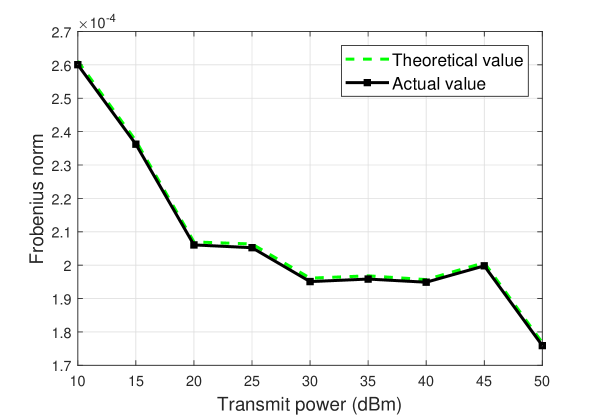
Figure 2: The differences between the Frobenius norm of the matrix ${\bm{\Sigma}}_{k}^{\left(1\right)}\left(i,j\right)$ in Theorem 1 and ${\beta_{i}}{\alpha_{j}}{\bm{\nu}}^{\textrm{H}}{{\bm{c}}^{ij}}$ obtained by our designed scheme.

Fig. 2 shows the differences between the Frobenius norm of the matrix ${\bm{\Sigma}}_{k}^{\left(1\right)}\left(i,j\right)$ in Theorem 1 and ${\beta_{i}}{\alpha_{j}}{\bm{\nu}}^{\textrm{H}}{{\bm{c}}^{ij}}$ obtained by our designed scheme. In this figure, we randomly select one user to compare its Frobenius norm of ${\beta_{i}}{\alpha_{j}}{\bm{\nu}}^{\textrm{H}}{{\bm{c}}^{ij}}$ with the F-norm of the theoretical value of diagonal matrix ${\bm{\Sigma}}_{k}^{\left(1\right)}\left(i,j\right)$ in Theorem 1. From this figure, we see that, the Frobenius norm of ${\bm{\Sigma}}_{k}^{\left(1\right)}\left(i,j\right)$ and ${\beta_{i}}{\alpha_{j}}{\bm{\nu}}^{\textrm{H}}{{\bm{c}}^{ij}}$ are very close, which verifies the correctness of Theorem 1. From Fig. 2, we can also see that, the F-norm of ${\bm{\Sigma}}_{k}^{\left(1\right)}\left(i,j\right)$ and ${\beta_{i}}{\alpha_{j}}{\bm{\nu}}^{\textrm{H}}{{\bm{c}}^{ij}}$ fluctuates up and down with the change of the transmit power. This implies that the singular values of the mmWave effective channel are not affected by the transmit power.

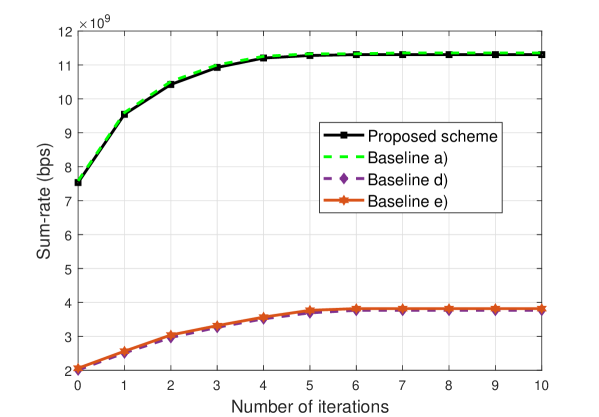
Figure 3: Convergence of the considered algorithms for sovling problem (28).

Fig. 3 shows the convergence of the proposed algorithm to solve problem (28). From Fig. 3, we observe that, the proposed algorithm can achieve up to 2x and 2x gains in terms of the sum of all users’ data rates compared to baselines d) and e). This is due to the fact that, our proposed BD method can eliminate the inter-group interference. From Fig. 3, we can also see that, the number of iterations that the proposed algorithm needs to converge is similar to that of baseline a). This implies that the proposed algorithm that uses hybrid beamforming can reduce energy consumption without increasing the complexity of finding optimal solution for serving users. Fig. 3 also shows that, the proposed scheme only needs seven iterations to solve problem (28), which further verifies the quick convergence speed of the designed scheme.

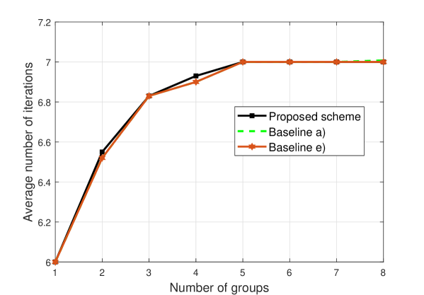
Figure 4: The average number of iterations versus number of groups.

Fig. 4 shows how the average number of iterations that the considered algorithms need to convergence changes as the number of groups varies. From Fig. 4, we see that, as the number of groups increases, the average number of iterations that the considered algorithms need to converge increases. This is due to the fact that, as the number of groups increases, the considered algorithms require more iterations to find the optimal phase shifts of the IRS. As the number of groups continues to increase, the average number of iterations for convergence remains constant. This is because the BS has enough user groups to determine the phase shifts of the IRS. From Fig. 4, we can also see that, the average number of iterations that the proposed algorithm needs to converge is similar to that of baselines a) and e). This implies that the proposed algorithm can reduce the hardware implementation complexity without increasing the complexity of finding optimal solution for serving users.

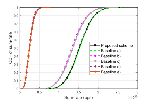
Figure 5: CDF of sum-rate.

Fig. 5 shows the cumulative distribution function (CDF) of the sum-rate of all users when the transmit power of the BS is 40 dBm. From Fig. 5, we can see that the proposed scheme improves the CDF of up to 81.8% and 78.33% gains compared to baselines b) and c) when the sum of all users’ data rates is 15 Gbps. This is because the phase shifts of the proposed scheme are optimized, resulting in high gain of the effective channel, which further facilitates the selection of the transmit beamforming matrices of the BS and the receive beamforming matrices of the users.

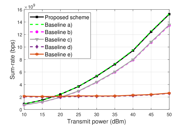
Figure 6: Sum-rate changes as the transmit power of the BS.

Fig. 6 shows how the sum rate of all users changes as the transmit power of the BS varies. From Fig. 6, we see that, the performance achieved by the proposed algorithm is similar to the optimal performance achieved by baseline a). This is because the proposed shceme can find the optimal hybrid beamforming matrices to represent the fully digital matrices. Fig. 6 also shows that compared to baselines b) and d), the proposed scheme can achieve up to 13% and 5x gains in terms of the sum rate of all users when $P$=50 dBm and $M$=256. This is because the proposed scheme optimizes the phase shifts of the IRS by a manifold method and eliminate the interference by the BD method. From Fig. 6, we can also see that, as the transmit power of the BS increases, the sum rate of baselines d) and e) remains unchanged. This is due to the fact that baselines d) and e) do not eliminate inter-group interference, which increases as the transmit power of the BS increases.

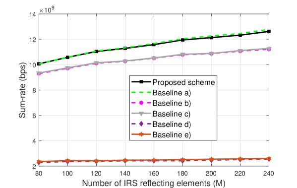
Figure 7: Sum-rate versus number of reflecting elements at the IRS.

In Fig. 7, we show how the sum of all users’ data rates changes as the number of reflecting elements at the IRS varies. Fig. 7 shows that the proposed scheme can achieve up to 13.3% and 4x gains in terms of the sum of all users’ data rates compared to baselines b) and d) when $M$=240. This is due to the fact that the proposed scheme can align the angles of the cascaded channel and improve SINR. Fig. 7 also shows that as the number of reflection elements of the IRS increases, the performance of baselines d) and e) is remains unchanged. This is because baselines d) and e) only eliminate the self-interference of each user without eliminating the inter-group interference.

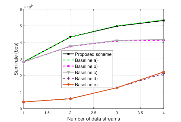
Figure 8: Sum-rate versus number of data streams.

In Fig. 8, we show how the sum of all users’ data rates changes as the number of data streams changes. From this figure, we can see that, as the number of data streams increases, the sum-rate of all considered algorithms increases. This is due to the fact that the desired signal power increases as the number of data streams increases. Fig. 8 also shows that the proposed scheme can achieve up to 28.6% and 152.97% gains in terms of the sum of all users’ data rates compared to baselines b) and d) when the number of data streams is 4. This is because our proposed BD method can eliminate the inter-group interference and the self-interference of each user, and the manifold method can find the suitable IRS phase shifts.

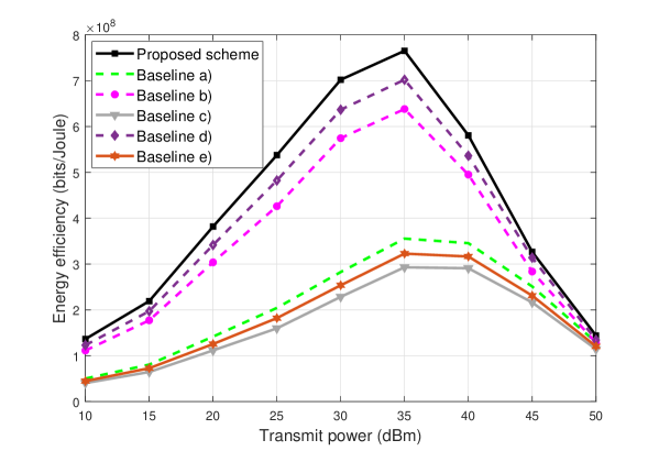
Figure 9: Energy efficiency versus the transmit power of the BS.

Fig. 9 shows how the energy efficiency changes as the transmission power of the BS varies. In this figure, the energy efficiency is defined as the ratio of the sum-rate to the total power consumption of the system. The total power consumption of the system includes the transmission power at the BS, the hardware static power consumption at the BS, and the hardware static power consumption of the each reflecting element at the IRS. From Fig. 9, we can see that, the proposed scheme can achieve up to 19.92% gain in terms of energy efficiency compared to baseline b). This is due to the fact that the proposed algorithm optimizes the phase shift to align the angle of the path from the BS to the users. From Fig. 9, we can also see that the proposed scheme can achieve up to 9% gain in terms of energy efficiency compared to baseline d). This is because the proposed BD method eliminates both the inter-group interference and the self-interference, while baseline d) only eliminates the self-interference of each user. Fig. 9 also shows that the energy efficiency increases when the transmit power of the BS is less than 35 dBm. However, when the transmit power of the BS is higher than 35 dBm, the energy efficiency decreases. This is due to the fact that, as the transmit power of the BS increases, the total power consumption of the system increases.

V Conclusions

In this paper, we have developed a novel framework for an IRS-assisted mmWave multigroup multicast MIMO communication system. The transmit beamforming matrices of the BS, the receive beamforming matrices of the users, and the phase shifts of the IRS were jointly optimized to maximize the sum rate of all users. We have used a BD method to represent the beamforming matrices of the BS and the users in terms of the IRS phase shifts. Then, we have transformed the original problem to a problem that only needs to optimize the IRS phase shifts. The transformed problem is solved by a manifold method. Simulation results show that the proposed scheme can achieve significant performance gains compared to baselines.

Appendix A

To prove Theorem 1, we first define the effective channel ${\bm{H}}_{k}$ as done in [15]:

$$\vspace{-.5em}{\bm{H}}_{k}={G_{\textrm{t}}}{G_{\textrm{r}}}\bm{H}^{\textrm{R}}_{k}\bm{\Phi}\bm{H}^{\textrm{B}}=\bm{A}_{k}\bm{D}_{k}\left(\bm{A}\right)^{\textrm{H}},$$ (44)

where $\bm{A}_{k}=\left[\bm{a}\left(r_{1,k}^{\textrm{A}}\right),\ldots,\bm{a}\left(r_{L,k}^{\textrm{A}}\right)\right]$ is a array response matrix of user $k$, $\bm{A}=\left[\bm{a}\left(r_{1}^{\textrm{D}}\right),\ldots,\bm{a}\left(r_{Y}^{\textrm{D}}\right)\right]$ is a array response matrix of the BS, and $\bm{D}_{k}$ is an $Y\times L$ matrix with element $\bm{D}_{k}\left(i,j\right)={\beta_{i}}{\alpha_{j}}{d_{ij}}$, where ${d_{ij}}$ can be given by

$$\begin{split}{d_{ij}}&=\left(\bm{a}\left({\theta}_{i}^{{\textrm{D}}},{\eta}_{i}^{{\textrm{D}}}\right)\right)^{{\textrm{H}}}\bm{\Phi}\bm{a}\left({\theta}_{j}^{{\textrm{A}}},{\eta}_{j}^{{\textrm{A}}}\right)\\ &={\bm{\nu}}^{\textrm{H}}\left(\left(\bm{a}\left({\theta}_{i}^{{\textrm{D}}},{\eta}_{i}^{{\textrm{D}}}\right)\right)^{{\textrm{*}}}\circ\bm{a}\left({\theta}_{j}^{{\textrm{A}}},{\eta}_{j}^{{\textrm{A}}}\right)\right)\\ &={\bm{\nu}}^{\textrm{H}}{{\bm{c}}^{ij}}.\end{split}$$ (45)

Given the effective channel ${\bm{H}}_{k}$, we define $\tilde{\bm{H}}_{h}$ as

$$\begin{split}&\tilde{\bm{H}}_{h}=\left[{\bm{H}}_{1},\ldots,{\bm{H}}_{h-1},{\bm{H}}_{h+1},\ldots,{\bm{H}}_{H}\right]^{\textrm{T}},\\ &=\quad~{}~{}~{}~{}\quad\quad\left[\begin{matrix}\bm{A}_{1}{\bm{D}_{1}}{\left(\bm{A}\right)^{{\textrm{H}}}}&\\ \bm{A}_{2}{\bm{D}_{2}}{\left(\bm{A}\right)^{{\textrm{H}}}}&\\ \vdots&\\ \bm{A}_{K}{\bm{D}_{K}}{\left(\bm{A}\right)^{{\textrm{H}}}}\end{matrix}\!\!\!\!\!\right],\\ &=\left[\begin{matrix}\bm{A}_{1}&\cdots&0&\\ \vdots&\ddots&\vdots&\\ 0&\cdots&\bm{A}_{K}\end{matrix}\!\!\!\!\!\right]\left[\begin{matrix}\bm{D}_{1}&\cdots&0&\\ \vdots&\ddots&\vdots&\\ 0&\cdots&\bm{D}_{K}\end{matrix}\!\!\!\!\!\right]\left[\begin{matrix}\left(\bm{A}\right)^{{\textrm{H}}}\\ \vdots\\ \left(\bm{A}\right)^{{\textrm{H}}}\end{matrix}\!\right],\\ &=\left[\begin{matrix}\bm{A}_{1}&\cdots&0&\\ \vdots&\ddots&\vdots&\\ 0&\cdots&\bm{A}_{K}\end{matrix}\!\!\!\!\!\right]\bm{P}\left[\begin{matrix}\tilde{\bm{\Sigma}}&\bm{0}&\\ \bm{0}&\bm{0}&\end{matrix}\!\!\!\!\!\right]\bm{Q}\left[\begin{matrix}\left(\bm{A}\right)^{{\textrm{H}}}\\ \vdots\\ \left(\bm{A}\right)^{{\textrm{H}}}\end{matrix}\!\right].\end{split}$$ (46)

We define $\bm{Q}\left[\begin{matrix}\left(\bm{A}\right)^{{\textrm{H}}}\\ \vdots\\ \left(\bm{A}\right)^{{\textrm{H}}}\end{matrix}\!\right]$ as ${\bm{Z}}$, hence, $\tilde{\bm{V}}_{h}^{\left(0\right)}=\left[\bm{z}_{\left(K-{\left|\mathcal{H}_{h}\right|}\right){\zeta}+1};\ldots;\bm{z}_{K{\zeta}}\right]$, with $\bm{z}_{\left(K-{\left|\mathcal{H}_{h}\right|}\right){\zeta}+1}$ being row ${\left(K-{\left|\mathcal{H}_{h}\right|}\right){\zeta}+1}$ of matrix ${\bm{Z}}$. Based on (44), ${\bm{H}}_{k}\tilde{\bm{V}}_{h}^{\left(0\right)}$ is given by

$${\bm{H}}_{k}\tilde{\bm{V}}_{h}^{\left(0\right)}=\bm{A}_{k}\bm{D}_{k}\left(\bm{A}\right)^{{\textrm{H}}}\left[\bm{z}_{\left(K-{\left|\mathcal{H}_{h}\right|}\right){\zeta}+1};\ldots;\bm{z}_{K{\zeta}}\right].$$ (47)

For ULA with $N$ antennas, the column vectors of $\bm{A}_{k}$ and row vectors of $\left(\bm{A}\right)^{{\textrm{H}}}\left[\bm{z}_{\left(K-{\left|\mathcal{H}_{h}\right|}\right){\zeta}+1};\ldots;\bm{z}_{K{\zeta}}\right]$ can form orthonormal sets[15]. Hence, ${\bm{H}}_{k}\tilde{\bm{V}}_{h}^{\left(0\right)}=\bm{A}_{k}\bm{D}_{k}\left(\bm{A}\right)^{{\textrm{H}}}\left[\bm{z}_{\left(K-{\left|\mathcal{H}_{h}\right|}\right){\zeta}+1};\ldots;\bm{z}_{K{\zeta}}\right]$ can be considered as an approximation of the truncated SVD of ${\bm{H}}_{k}\tilde{\bm{V}}_{h}^{\left(0\right)}$, and $\bm{D}_{k}$ can represent ${\bm{\Sigma}}_{k}^{\left(1\right)}$.

References

• [1] A. L. Swindlehurst, E. Ayanoglu, P. Heydari, and F. Capolino, “Millimeter-wave massive MIMO: The next wireless revolution?” IEEE Communications Magazine, vol. 52, no. 9, pp. 56–62, Sep. 2014.
• [2] J. Sun, M. Jia, Q. Guo, X. Gu, and Y. Gao, “Power distribution based beamspace channel estimation for mmWave massive MIMO system with lens antenna array,” IEEE Transactions on Wireless Communications, to appear, 2022.
• [3] J. Wang, X. Zhang, X. Shi, and J. Song, “Higher spectral efficiency for mmWave MIMO: Enabling techniques and precoder designs,” IEEE Communications Magazine, vol. 59, no. 4, pp. 116–122, Apr. 2021.
• [4] W. Wang and A. Leshem, “Non-convex generalized nash games for energy efficient power allocation and beamforming in mmWave networks,” IEEE Transactions on Signal Processing, vol. 70, pp. 3193–3205, Jun. 2022.
• [5] T. S. Rappaport, S. Sun, R. Mayzus, H. Zhao, Y. Azar, K. Wang, G. N. Wong, J. K. Schulz, M. Samimi, and F. Gutierrez, “Millimeter wave mobile communications for 5G cellular: It will work!” IEEE Access, vol. 1, pp. 335–349, May 2013.
• [6] C. Qi, Q. Liu, X. Yu, and G. Y. Li, “Hybrid precoding for mixture use of phase shifters and switches in mmWave massive MIMO,” IEEE Transactions on Communications, vol. 70, no. 6, pp. 4121–4133, Jun. 2022.
• [7] I. Ahmed, H. Khammari, A. Shahid, A. Musa, K. S. Kim, E. De Poorter, and I. Moerman, “A survey on hybrid beamforming techniques in 5G: Architecture and system model perspectives,” IEEE Communications Surveys and Tutorials, vol. 20, no. 4, pp. 3060–3097, Fourthquarter 2018.
• [8] Z. Yang, M. Chen, W. Saad, W. Xu, M. Shikh-Bahaei, H. V. Poor, and S. Cui, “Energy-efficient wireless communications with distributed reconfigurable intelligent surfaces,” IEEE Transactions on Wireless Communications, vol. 21, no. 1, pp. 665–679, Jan. 2022.
• [9] C. Huang, A. Zappone, G. C. Alexandropoulos, M. Debbah, and C. Yuen, “Reconfigurable intelligent surfaces for energy efficiency in wireless communication,” IEEE Transactions on Wireless Communications, vol. 18, no. 8, pp. 4157–4170, Aug. 2019.
• [10] S. Liu, Z. Gao, J. Zhang, M. D. Renzo, and M.-S. Alouini, “Deep denoising neural network assisted compressive channel estimation for mmWave intelligent reflecting surfaces,” IEEE Transactions on Vehicular Technology, vol. 69, no. 8, pp. 9223–9228, Aug. 2020.
• [11] E. E. Bahingayi and K. Lee, “Low-complexity beamforming algorithms for IRS-aided single-user massive MIMO mmWave systems,” IEEE Transactions on Wireless Communications, to appear, 2022.
• [12] F. Yang, J.-B. Wang, H. Zhang, M. Lin, and J. Cheng, “Intelligent reflecting surface assisted mmWave communication using mixed timescale channel state information,” IEEE Transactions on Wireless Communications, vol. 21, no. 7, pp. 5673–5687, Jul. 2022.
• [13] H. Du, J. Zhang, J. Cheng, and B. Ai, “Millimeter wave communications with reconfigurable intelligent surfaces: Performance analysis and optimization,” IEEE Transactions on Communications, vol. 69, no. 4, pp. 2752–2768, Apr. 2021.
• [14] P. Wang, J. Fang, X. Yuan, Z. Chen, and H. Li, “Intelligent reflecting surface-assisted millimeter wave communications: Joint active and passive precoding design,” IEEE Transactions on Vehicular Technology, vol. 69, no. 12, pp. 14 960–14 973, Dec. 2020.
• [15] P. Wang, J. Fang, L. Dai, and H. Li, “Joint transceiver and large intelligent surface design for massive MIMO mmWave systems,” IEEE Transactions on Wireless Communications, vol. 20, no. 2, pp. 1052–1064, Feb. 2021.
• [16] C. Pradhan, A. Li, L. Song, B. Vucetic, and Y. Li, “Hybrid precoding design for reconfigurable intelligent surface aided mmWave communication systems,” IEEE Wireless Communications Letters, vol. 9, no. 7, pp. 1041–1045, Jul. 2020.
• [17] K. Ying, Z. Gao, S. Lyu, Y. Wu, H. Wang, and M.-S. Alouini, “GMD-based hybrid beamforming for large reconfigurable intelligent surface assisted millimeter-wave massive MIMO,” IEEE Access, vol. 8, pp. 19 530–19 539, Jan. 2020.
• [18] W. Zhang, J. Xu, W. Xu, D. W. K. Ng, and H. Sun, “Cascaded channel estimation for IRS-assisted mmWave multi-antenna with quantized beamforming,” IEEE Communications Letters, vol. 25, no. 2, pp. 593–597, Feb. 2021.
• [19] H. Xie, J. Xu, and Y.-F. Liu, “Max-min fairness in IRS-aided multi-cell MISO systems with joint transmit and reflective beamforming,” IEEE Transactions on Wireless Communications, vol. 20, no. 2, pp. 1379–1393, Feb. 2021.
• [20] G. Zhou, C. Pan, H. Ren, K. Wang, and M. D. Renzo, “Fairness-oriented multiple RIS-aided mmWave transmission: Stochastic optimization methods,” IEEE Transactions on Signal Processing, vol. 70, pp. 1402–1417, Mar. 2022.
• [21] F. Yang, J.-B. Wang, H. Zhang, M. Lin, and J. Cheng, “Multi-IRS-assisted mmWave MIMO communication using twin-timescale channel state information,” IEEE Transactions on Communications, to appear, 2022.
• [22] H. Niu, Z. Chu, F. Zhou, C. Pan, D. W. K. Ng, and H. X. Nguyen, “Double intelligent reflecting surface-assisted multi-user MIMO mmWave systems with hybrid precoding,” IEEE Transactions on Vehicular Technology, vol. 71, no. 2, pp. 1575–1587, Feb. 2022.
• [23] B. Zheng, C. You, and R. Zhang, “Double-IRS assisted multi-user MIMO: Cooperative passive beamforming design,” IEEE Transactions on Wireless Communications, vol. 20, no. 7, pp. 4513–4526, Jul. 2021.
• [24] W. Huang, Y. Huang, S. He, and L. Yang, “Cloud and edge multicast beamforming for cache-enabled ultra-dense networks,” IEEE Transactions on Vehicular Technology, vol. 69, no. 3, pp. 3481–3485, Mar. 2020.
• [25] W. Ci, C. Qi, G. Y. Li, and S. Mao, “Hybrid beamforming design for covert multicast mmWave massive MIMO communications,” in Proc. IEEE Global Communications Conference, Madrid, Spain, Dec. 2021, pp. 1–6.
• [26] Z. Zhang, Z. Ma, Y. Xiao, M. Xiao, G. K. Karagiannidis, and P. Fan, “Non-orthogonal multiple access for cooperative multicast millimeter wave wireless networks,” IEEE Journal on Selected Areas in Communications, vol. 35, no. 8, pp. 1794–1808, Aug. 2017.
• [27] Q. Tao, S. Zhang, C. Zhong, and R. Zhang, “Intelligent reflecting surface aided multicasting with random passive beamforming,” IEEE Wireless Communications Letters, vol. 10, no. 1, pp. 92–96, Jan. 2021.
• [28] G. Zhou, C. Pan, H. Ren, K. Wang, and A. Nallanathan, “Intelligent reflecting surface aided multigroup multicast MISO communication systems,” IEEE Transactions on Signal Processing, vol. 68, pp. 3236–3251, Apr. 2020.
• [29] L. Du, S. Shao, G. Yang, J. Ma, Q. Liang, and Y. Tang, “Capacity characterization for reconfigurable intelligent surfaces assisted multiple-antenna multicast,” IEEE Transactions on Wireless Communications, vol. 20, no. 10, pp. 6940–6953, Oct. 2021.
• [30] L. Du, W. Zhang, J. Ma, and Y. Tang, “Reconfigurable intelligent surfaces for energy efficiency in multicast transmissions,” IEEE Transactions on Vehicular Technology, vol. 70, no. 6, pp. 6266–6271, Jun. 2021.
• [31] H. Kasai, “Fast optimization algorithm on complex oblique manifold for hybrid precoding in millimeter wave MIMO systems,” in Proc. IEEE Global Conference on Signal and Information Processing, Anaheim, USA, Nov. 2018, pp. 1266–1270.
• [32] X. Yu, J.-C. Shen, J. Zhang, and K. B. Letaief, “Alternating minimization algorithms for hybrid precoding in millimeter wave MIMO systems,” IEEE Journal of Selected Topics in Signal Processing, vol. 10, no. 3, pp. 485–500, Apr. 2016.
• [33] O. E. Ayach, S. Rajagopal, S. Abu-Surra, Z. Pi, and R. W. Heath, “Spatially sparse precoding in millimeter wave MIMO systems,” IEEE Transactions on Wireless Communications, vol. 13, no. 3, pp. 1499–1513, Mar. 2014.
• [34] P.-A. Absil, R. Mahony, and R. Sepulchre, Optimization Algorithms on Matrix Manifolds.   Princeton University Press, 2009.
• [35] D. Xu, X. Yu, Y. Sun, D. W. K. Ng, and R. Schober, “Resource allocation for secure IRS-assisted multiuser MISO systems,” in Proc. IEEE Global Communications Conference Workshops, Waikoloa, HI, USA, Dec. 2019, pp. 1–6.