On minimum contrast method for multivariate spatial point processes

Abstract

Compared to widely used likelihood-based approaches, the minimum contrast (MC) method is a computationally efficient method for estimation and inference of parametric stationary point processes. This advantage becomes more pronounced when analyzing complex point process models, such as multivariate log-Gaussian Cox processes (LGCP). Despite its practical advantages, there is very little work on the MC method for multivariate point processes. The aim of this article is to introduce a new MC method for parametric multivariate stationary spatial point processes. A contrast function is calculated based on the trace of the power of the difference between the conjectured $K$-function matrix and its nonparametric unbiased edge-corrected estimator. Under standard assumptions, the asymptotic normality of the MC estimator of the model parameters is derived. The performance of the proposed method is illustrated with bivariate LGCP simulations and a real data analysis of a bivariate point pattern of the 2014 terrorist attacks in Nigeria.

Keywords: Log-Gaussian Cox process; marginal and cross $K$-function; minimum contrast method; multivariate spatial point process; optimal control parameters.

1 Introduction

A multivariate spatial point pattern is comprised of a random number of events at random locations in a given spatial region $D\subset\mathbb{R}^{d}$ (where $d$ is usually set to 2 or 3), where each event belongs to one (and only one) of a finite number of distinct “types” (Cox and Lewis, 1972). These “presence only” data have become increasingly common, with multivariate spatial point patterns now found in a variety of disciplines including epidemiology (Lawson, 2012), neuroscience (Baddeley et al., 2014), ecology (Waagepetersen et al., 2016), meteorology (Jun et al., 2019), and political science (Jun and Cook, 2022). Therefore, to better understand the spatial patterns of these multi-type events in real-life applications, it is important to develop effective statistical methods to analyze the multivariate spatial point process.

Maximum likelihood estimation (MLE) is a widely used approach to estimate and infer the parameters of spatial point processes. This is because the resulting MLE estimator has desirable large sample properties (Ogata, 1978; Helmers and Zitikis, 1999; Karr, 2017). However, one of the biggest challenges with MLE is that the likelihood function of a spatial point process is, in general, analytically intractable. As such, MLE requires an appropriate approximation for the likelihood function. For example, in log-Gaussian Cox processes (LGCP; Møller et al., 1998), the (intractable) likelihood function involves the expectation with respect to the log of the latent stochastic intensity process. To approximate this expected value, and in turn, approximate the likelihood function, one can use Monte Carlo simulation as in Jun et al. (2019). Alternatively, Bayesian inferential methods (e.g., Rue et al., 2009; Girolami and Calderhead, 2011) can be implemented to obtain the approximation of the likelihood function of an LGCP model.

However, these likelihood approximation methods pose some challenges in application. First, they require researchers to specify the point process models (e.g., LGCPs or Gibbs point processes) and appropriately modify the algorithms accordingly when considering alternative models. Second, as the model becomes increasingly complex or the number of computational grids increases, the aforementioned likelihood approximation methods are computationally intensive. Specifically, drawing each sample of model parameters and latent random fields on dense grids (in Monte Carlo simulations) or running long iterations to reach the convergence of the Markov chain (in Bayesian methods) is computationally demanding. We mention that, to handle these computational issues, several pseudo likelihood or composite likelihood approximation methods for point processes are proposed, such as Jalilian et al. (2015) for Cox processes and Rajala et al. (2018) for Gibbs point processes.

As an alternative to these likelihood-based methods, Minimum Contrast (MC; Diggle and Gratton, 1984) estimation is a computationally efficient inferential method for spatial point processes. The MC estimation selects the model parameters which minimize the discrepancy between the conjectured “descriptor” of point processes and its nonparametric estimator. For univariate point processes, a typical choice of a descriptor function is Ripley’s $K$-function (Ripley, 1976) or pair correlation function (PCF). This is because an analytic form of the $K$-function and PCF are available for many point process models, including LGCP, and more generally, shot noise Cox process (Møller, 2003).

To elaborate the MC method, let $Q(\cdot;\bm{\theta})$, $\bm{\theta}\in\Theta$, be a family of parametric descriptors of stationary point process and $\widehat{Q}(\cdot)$ be its estimator. Then, MC estimation aims to minimize the “integrated distance” between $Q(\cdot;\bm{\theta})$ and $\widehat{Q}(\cdot)$ over the prespecified domain. For instance, if a univariate point process has the parametric $K$-function as its descriptor function, that is, $Q(h;\bm{\theta})=K(h;\bm{\theta})$ for $h\in[0,\infty)$, then the MC estimator is defined as

$$\widehat{\bm{\theta}}=\operatorname*{arg\,min}_{\bm{\theta}\in\Theta}\mathcal{U}(\bm{\theta})\quad\text{where}\quad\mathcal{U}(\bm{\theta})=\int_{0}^{R}w(h)\left\{|K(h;\bm{\theta})|^{c}-|\widehat{K}(h)|^{c}\right\}^{2}dh.$$ (1.1)

Here, $R$ is a positive range, $w(\cdot)$ is a non-negative weight function, $K(\cdot;\bm{\theta})$ and $\widehat{K}(\cdot)$ are parametric $K$-function and its nonparametric estimator (see Section 3.1 for the precise definitions), and $c\in[0,\infty)$ is a non-negative power. Given its form in (1.1), provided that $K(h;\bm{\theta})$ has a known form and $\widehat{K}(h)$ can be easily evaluated for all $h\in[0,\infty)$, the MC estimator can be easily obtained by using standard numerical optimization methods. This computational advantage becomes more pronounced when working with complex point processes which are challenging for likelihood-based methods. As such, the MC method has been used extensively to analyze the univariate point processes in applications (e.g., Møller et al., 1998; Møller and Waagepetersen, 2007; Guan, 2009; Møller and Díaz-Avalos, 2010; Davies and Hazelton, 2013; Cui et al., 2018). There have also been developments in our theoretical understanding of these univariate point processes. For example, Heinrich (1992) studied the asymptotic properties of the MC estimator for univariate homogeneous Poisson processes (Kingman, 1992) with $c=0.5$ and Guan and Sherman (2007) extended the distribution theory of the MC estimator to a fairly large class of univariate point process models.

Despite the increasing use of the univariate MC method in applications, there is very little work on MC methods for multivariate point processes in both theory and application. This is because, unlike the univariate model, for multiple potentially related point patterns, one also needs to examine the cross-group interactions (or even the higher-order interactions) between the different types of point processes. Therefore, the descriptor function $Q(\cdot;\bm{\theta})$ is no longer a functional, but instead a matrix- or tensor-valued function. This requires the development of a new way to measure the discrepancy between these types of functions. Waagepetersen et al. (2016), for example, proposed the least square estimation of the parametric multivariate LGCP model and applied the method to real-world data on forest ecology. However, their method is tied to the specific structure of the multivariate LGCP models and there is no theoretical justification for the estimator.

In this article, we extend over existing research on MC estimation for multivariate point processes in at least three ways. First, we offer a new MC method to analyze the fairly large class of multivariate stationary point processes, which does not necessaraily assume that the logarithm of the latent intensity is a Gaussian process. In Section 3.2, we propose a new discrepancy measure between the $m\times m$ matrix-valued scaled $K$-function and its nonparametric unbiased estimator (see, (3.11) for the precise form). Second, under the increasing-domain asymptotic framework (Jensen, 1993; Guan and Sherman, 2007; Fuentes-Santos et al., 2016), we derive the asymptotic normality of the MC estimator which minimizes the proposed contrast function (see, Theorem 4.2). Finally, based on the asymptotic results, we propose a method to select the optimal control parameters of the MC method (see, Sections 5.1 and 5.2).

The rest of this article is organized as follows. In Section 2, we provide background knowledge on the spatial point process and define the higher-order “joint” intensity function of a multivariate spatial point process. In Section 3.1, we introduce the marginal and cross $K$-functions and their nonparametric estimators. Using these $K$-function estimators, in Section 3.2, we define a new discrepancy measure between the two matrix-valued functions. In Section 4, we investigate large sample properties of the the MC estimator. In Section 5, we consider the practical application of the MC estimator including estimation of asymptotic covariance matrix (Section 5.1) and selection of the optimal control parameters (Section 5.2). We consider the bivariate LGCP model that is used in simulations (Section 6) and a real data analysis of terrorism attacks in Section 7. In Section 8, we discuss further extension of our methods. Finally, auxiliary results, proofs, and additional figures and tables can be found in the Appendix.

2 Joint intensity functions of multivariate point processes

In this section, we introduce the joint intensity functions of $m$-tuple of point processes. To do so, we will briefly review some background concepts that are used throughout this article. For greater detail on the mathematical presentations of point processes we refer readers to Daley and Vere-Jones (2003, 2008), and Baddeley et al. (2007).

Let $X$ be a spatial point process defined on $\mathbb{R}^{d}$, where we observe the sample of $X$ in $D\subset\mathbb{R}^{d}$. For a bounded Borel set $E\subset D$, $N_{X}(E)$ denotes the random variable that counts the number of events of $X$ within $E$. For $n\in\mathbb{N}$, let $\lambda_{n}:D^{n}\mapsto\mathbb{R}$ be the $n$th-order intensity function (also known as the product density function) of $X$. Thus,

$$\lambda_{n}(\bm{x}_{1},\cdots,\bm{x}_{n})=\lim_{|d\bm{x}_{1}|,\cdots,|d\bm{x}_{n}|\rightarrow 0}\frac{\mathbb{E}\left[N_{X}(d\bm{x}_{1})\cdots N_{X}(d\bm{x}_{n})\right]}{|d\bm{x}_{1}|\cdots|d\bm{x}_{n}|},\quad\bm{x}_{1}\neq\bm{x}_{2}\cdots\neq\bm{x}_{n}\in D,$$ (2.1)

and zero otherwise. Here, $\bm{x}_{1}\neq\bm{x}_{2}\cdots\neq\bm{x}_{n}\in D$ denotes the $n$ pairwise distinct points in $D$ and for $i\in\{1,\dots,n\}$, $d\bm{x}_{i}$ denotes the infinitesimal region in $D$ that contains $\bm{x}_{i}\in D$ and $|d\bm{x}_{i}|$ denotes the volume of $d\bm{x}_{i}$. If we further assume that $X$ is stationary, then we can write $\lambda_{1}(\bm{x}_{1})=\lambda_{1}$ for all $\bm{x}_{1}\in D$ and

$$\lambda_{n}(\bm{x}_{1},\cdots,\bm{x}_{n})=\lambda_{n,\text{red}}(\bm{x}_{2}-\bm{x}_{1},\cdots,\bm{x}_{n}-\bm{x}_{1}),\quad n\in\{2,3,\cdots\}\quad\text{and}\quad\bm{x}_{1},\dots,\bm{x}_{n}\in D.$$ (2.2)

We refer to $\lambda_{n,\text{red}}$ as the $n$-th order reduced intensity function of $X$.

For a multivariate point process defined on the same probability space and the same sampling window, we can naturally extend the definition of the $n$th-order intensity function for univarite spatial point processes.

Definition 2.1 (Joint intensity functions of multivariate point processes)

Let $\underline{X}=(X_{1},\cdots,X_{m})$ be an $m$-variate spatial point process defined on the same probability space. Let $D\subset\mathbb{R}^{d}$ be the common sampling window of $\underline{X}$. Denote $\underline{n}=(n_{1},\dots,n_{m})$ as an ordered set of non-negative deterministic integers and $\underline{\bm{x}}=(\underline{\bm{x}}_{1},\dots,\underline{\bm{x}}_{m})$ as an ordered vector where $\underline{\bm{x}}_{i}=(\bm{x}_{i,1},\cdots,\bm{x}_{i,n_{i}})\in D^{n_{i}}$ for $i\in\{1,\dots,m\}$. The joint intensity function of $\underline{X}$ of order $\underline{n}$, denotes $\lambda_{\underline{n}}:D^{N}\mapsto\mathbb{R}$ (where $N=\sum_{i=1}^{m}n_{i}$), is defined as

$$\lambda_{\underline{n}}(\underline{\bm{x}})=\lim_{|d\bm{x}_{1,1}|,\cdots,|d\bm{x}_{m,n_{m}}|\rightarrow 0}\frac{\mathbb{E}\left[\prod_{j=1}^{n_{1}}N_{X_{1}}(d\bm{x}_{1,j})\times\cdots\times\prod_{j=1}^{n_{m}}N_{X_{m}}(d\bm{x}_{m,j})\right]}{\prod_{j=1}^{n_{1}}|d\bm{x}_{1,j}|\times\cdots\times\prod_{j=1}^{n_{m}}|d\bm{x}_{m,j}|}$$ (2.3)

for $\bm{x}_{i,1}\neq\cdots\neq\bm{x}_{i,n_{i}}\in D$, $i\in\{1,\dots,m\}$, and zero otherwise. Following convention, we let $\prod_{1}^{0}=1$. Sometimes, it will be necessary to consider the joint intensity of the subset of $\underline{X}$. In this case, for an ordered non-overlapping index $\mathcal{I}=(i(1),\dots,i(k))\subset\{1,\dots,m\}$ and $\underline{n}=(n_{1},\dots,n_{k})$, we denote

$$\lambda^{\mathcal{I}}_{\underline{n}}(\underline{\bm{x}}_{1},\dots,\underline{\bm{x}}_{k})=\lim_{|d\bm{x}_{1,1}|,\cdots,|d\bm{x}_{k,n_{k}}|\rightarrow 0}\frac{\mathbb{E}\left[\prod_{j=1}^{n_{1}}N_{X_{i(1)}}(d\bm{x}_{1,j})\times\cdots\times\prod_{j=1}^{n_{k}}N_{X_{i(k)}}(d\bm{x}_{k,j})\right]}{\prod_{j=1}^{n_{1}}|d\bm{x}_{1,j}|\times\cdots\times\prod_{j=1}^{n_{k}}|d\bm{x}_{k,j}|}$$ (2.4)

as the joint intensity function of $(X_{i(1)},\dots,X_{i(k)})$ of order $\underline{n}$.

If $\underline{X}$ is stationary, then analogous to (2.2), we have

$$\lambda_{\underline{n}}(\underline{\bm{x}})=\lambda_{\underline{n},red}(\bm{x}_{1,2}-\bm{x}_{1,1},\cdots,\bm{x}_{1,n_{1}}-\bm{x}_{1,1},\bm{x}_{2,1}-\bm{x}_{1,1},\cdots,\bm{x}_{m,n_{m}}-\bm{x}_{1,1}):D^{N-1}\mapsto\mathbb{R},$$ (2.5)

where $N=\sum_{i=1}^{m}n_{i}$. We refer to $\lambda_{\underline{n}}$ as the reduced joint intensity function of $\underline{X}$ of order $\underline{n}$. For an ordered subset $\mathcal{I}=(i(1),\dots,i(k))\subset\{1,\dots,m\}$, the reduced joint intensity function of the subset process $(X_{i(1)},\dots,X_{i(k)})$, denotes $\lambda_{\underline{n},\text{red}}^{\mathcal{I}}$, can be defined similarly. As a special case, for a bivariate point process $\underline{X}=(X_{1},X_{2})$, let

$$\lambda_{1,1}^{(1,2)}(\bm{x}_{1},\bm{x}_{2})=\lim_{|d\bm{x}_{1}|,|d\bm{x}_{2}|\rightarrow 0}\frac{\mathbb{E}\left[N_{X_{1}}(d\bm{x}_{1})N_{X_{2}}(d\bm{x}_{2})\right]}{|d\bm{x}_{1}||d\bm{x}_{2}|},\qquad\bm{x}_{1},\bm{x}_{2}\in D.$$ (2.6)

We refer to $\lambda_{1,1}^{(1,2)}$ as the second-order cross intensity function of $X_{1}$ and $X_{2}$.

Finally, we introduce the joint cumulant intensity function, as we use this concept in the proof of the asymptotic normality of the target random variables (see Assumption 4.1). By replacing the expectation with the cumulant in (2.3), we define the joint cumulant intensity function of $\underline{X}$ of order $\underline{n}=(n_{1},\dots,n_{m})$ by

$$\gamma_{\underline{n}}(\underline{\bm{x}})=\lim_{|d\bm{x}_{1,1}|,\cdots,|d\bm{x}_{m,n_{m}}|\rightarrow 0}\frac{\text{Cum}\left\{N_{X_{1}}(d\bm{x}_{1,1}),\dots,N_{X_{1}}(d\bm{x}_{1,n_{1}}),N_{X_{2}}(d\bm{x}_{1,n_{2}}),\dots,N_{X_{m}}(d\bm{x}_{m,n_{m}})\right\}}{\prod_{j=1}^{n_{1}}|d\bm{x}_{1,j}|\times\cdots\times\prod_{j=1}^{n_{m}}|d\bm{x}_{m,j}|}$$ (2.7)

for $\bm{x}_{i,1}\neq\cdots\neq\bm{x}_{i,n_{i}}\in D$, $i\in\{1,\dots,m\}$, and zero otherwise. Analogous to (2.5), if $\underline{X}$ is stationary, then

$$\gamma_{\underline{n}}(\underline{\bm{x}})=\gamma_{\underline{n},red}(\bm{x}_{1,2}-\bm{x}_{1,1},\dots,\bm{x}_{1,n_{1}}-\bm{x}_{1,1},\bm{x}_{2,1}-\bm{x}_{1,1},\dots.,\bm{x}_{m,n_{m}}-\bm{x}_{1,1}).$$ (2.8)

We refer to $\gamma_{\underline{n},\text{red}}$ as the reduced joint cumulant intensity function. For a subset process $\underline{X}^{\mathcal{I}}=(X_{i(1)},\dots,X_{i(k)})$, we can define the joint cumulant intensity function of $\underline{X}^{\mathcal{I}}$, denotes $\gamma^{\mathcal{I}}_{\underline{n}}$, and the reduced joint cumulant intensity function of $\underline{X}^{\mathcal{I}}$, denotes $\gamma^{\mathcal{I}}_{\underline{n},\text{red}}$, in the same manner.

3 Minimum contrast for multivariate point processes

In this section, we use the marginal and cross $K$-function to formulate the minimum contrast method for multivariate point processes.

3.1 The marginal and cross $K$-function

The $K$-function is an important measure to quantify the second-order interaction between the two points. Following the heuristic definition in Cressie (1993)(page 615), the (marginal) $K$-function of a univariate stationary point process $X$ is defined as

$$K(r):=\lambda_{1}^{-1}\mathbb{E}\Bigl{\{}\text{Number of distinct points within distance $r$ of a given point}\Bigr{\}},~{}~{}r\in[0,\infty),$$ (3.1)

where $\lambda_{1}$ is the homogeneous first-order intensity of $X$. A formal formulation of $K$-function based on the second-order reduced Palm measure can be found in Ripley (1976) and Baddeley et al. (2007) (Section 2.5).

Given a realization of $X$ sampled within $D_{n}\subset\mathbb{R}^{d}$ for $n\in\mathbb{N}$, a naive nonparametric estimator of $K(r)$ is

$$\widehat{K}_{0,n}(r)=\left(|D_{n}|{\hat{\lambda}_{1,n}}^{2}\right)^{-1}\sum_{\bm{x},\bm{y}\in X}\textbf{1}_{\{0<\|\bm{x}-\bm{y}\|\leq r\}},\quad r\in[0,\infty),\quad n\in\mathbb{N},$$ (3.2)

where $\hat{\lambda}_{1,n}=N_{X}(D_{n})/|D_{n}|$ is an unbiased estimator of the first-order intensity of $X$, $\textbf{1}_{\{\}}$ is the indicator function, and $\|\cdot\|$ is the euclidean norm. It is well-known that $\widehat{K}_{0,n}(r)$ is negatively biased since it neglects the undetected observations near the boundary of $D_{n}$. To amerliorate the boundary issue, we consider the edge-corrected estimator of $K(r)$, which can be written as the following general form:

$$\widehat{K}_{n}(r)=\left(|D_{n}|\hat{\lambda}_{1,n}^{2}\right)^{-1}\sum_{\bm{x},\bm{y}\in X}b(\bm{x},\bm{y})\textbf{1}_{\{0<\|\bm{x}-\bm{y}\|\leq r\}},\quad r\in[0,\infty),\quad n\in\mathbb{N}.$$ (3.3)

Here, $b(\cdot,\cdot)$ is an edge-correction factor which depends on the observation domain $D_{n}$ and radius $r$. In particular, we assume that $b(\cdot,\cdot)$ belongs one of the two commonly used edge-correction factors:

• Translation correction: we let $b_{1}(\bm{x},\bm{y})=|D_{n}|/|D_{n}\cap(D+\bm{x}-\bm{y})|$, where for set $A\subset\mathbb{R}^{d}$ and a point $\bm{x}\in\mathbb{R}^{d}$, $A+\bm{x}$ is defined as $\{\bm{y}:\bm{y}=\textbf{a}+\bm{x},~{}\textbf{a}\in A\}$.

• Minus Sampling correction: we let $b_{2}(\bm{x},\bm{y})=\{|D_{n}|/|D_{0n}|\}\textbf{1}_{\{\bm{x}\in D_{0n}\}}$, where

  $$D_{0n}=\{\bm{x}\in D_{n}:\text{there exits a distinct point }y\notin D_{n}\text{ such that }\|\bm{x}-\bm{y}\|>r\}.$$ (3.4)

  For example, if $D_{n}=B_{d}(\bm{x},s)$, a ball in $\mathbb{R}^{d}$ with the center $\bm{x}\in\mathbb{R}^{d}$ and radius $s>r$, then $D_{0n}=B_{d}(\bm{x},s-r)$.

If we further assume that the underlying point process $X$ is isotropic, then we consider the above two edge-correction factors plus the following edge-correction factor:

• Ripley’s edge-correction(Ripley, 1976): we let $b_{3}(\bm{x},\bm{y})=\lambda_{d-1}\{B_{d}(\bm{x},\|\bm{x}-\bm{y}\|)\}/\lambda_{d-1}\{B_{d}(\bm{x},\|\bm{x}-\bm{y}\|)\cap D_{n}\}$, where $\lambda_{d-1}\{\cdot\}$ is the $(d-1)$-dimensional surface measure.

We note that $b\in\{b_{1},b_{2}\}$ (or $b\in\{b_{1},b_{2},b_{3}\}$, assuming $X$ is isotropic) yields $\hat{\lambda}_{1,n}^{2}\widehat{K}_{n}(r)$ is an unbiased estimator of $\lambda_{1}^{2}K(r)$ for all $n\in\mathbb{N}$. For additional discussion on the various edge correction methods and their theoretical and empirical properties, we refer readers to Doguwa and Upton (1989), Cressie (1993)(pages 616–618), and Ang et al. (2012).

For a bivariate stationary point process, Hanisch and Stoyan (1979) extended the definition of (3.1) and defined the cross $K$-function of $(X_{i},X_{j})$ as

$$K_{ij}(r) = (\lambda^{(j)}_{1})^{-1}\mathbb{E}\Bigl{\{}\text{Number of (distinct) points of $X_{j}$}$$ (3.5)

$$\qquad\qquad\qquad\text{within distance $r$ of a given point of $X_{i}$}\Bigr{\}},\quad r\in[0,\infty),$$

where $\lambda^{(j)}_{1}$ is the (homogeneous) first-order intensity of $X_{j}$. The nonparametric edge-corrected estimator of $K_{ij}(r)$ within the sampling window $D_{n}\subset\mathbb{R}^{d}$ is

$$\widehat{K}_{ij,n}(r)=\left(|D_{n}|\hat{\lambda}_{1,n}^{(i)}\hat{\lambda}_{1,n}^{(j)}\right)^{-1}\sum_{\bm{x}\in X_{i}}\sum_{\bm{y}\in X_{j}}b(\bm{x},\bm{y})\textbf{1}_{\{\|\bm{x}-\bm{y}\|\leq r\}},\quad r\in[0,\infty),\quad n\in\mathbb{N},$$ (3.6)

where $\hat{\lambda}_{1,n}^{(i)}=N_{X_{i}}(D_{n})/|D_{n}|$ is the estimator of the (marginal) first-order intensity function of $X_{i}$ and $\hat{\lambda}_{1,n}^{(j)}$ is defined similarly for $X_{j}$. Then, if $b\in\{b_{1},b_{2}\}$ (or $b\in\{b_{1},b_{2},b_{3}\}$, provided that $(X_{i},X_{j})$ is jointly isotropic), then $\hat{\lambda}_{1,n}^{(i)}\hat{\lambda}_{1,n}^{(j)}\widehat{K}_{ij,n}(r)$ is an unbiased estimator for $\lambda_{1}^{(i)}\lambda_{1}^{(j)}K_{ij}(r)$.

3.2 The discrepancy measure and minimum contrast estimator

Let $\underline{X}=(X_{1},\dots,X_{m})$ be an $m$-variate stationary spatial point process. Our aim is to fit a parametric multivariate stationary spatial point process model with the marginal and cross $K$-functions to the observations. To set down the increasing domain asymptotic framework,we let the observations of $\underline{X}$ are made within the increasing sequence of sampling windows $\{D_{n}\}$ in $\mathbb{R}^{d}$, where $D_{1}\subset D_{2}\subset\dots$ and $\lim_{n\rightarrow\infty}|D_{n}|=\infty$.

Before introducing our discrepancy measure, we fix terms. Let

$$\bm{K}(r;\bm{\theta})=[K_{ij}(r;\bm{\theta})]_{i,j=1}^{m},\quad r\in[0,\infty),\quad\bm{\theta}\in\Theta,$$ (3.7)

be the $m\times m$ matrix-valued family of parametric $K$-functions, where for $i,j\in\{1,\dots,m\}$, $K_{ij}(\cdot,\bm{\theta})$ is the conjectured marginal $K$-function of $X_{i}$ (if $i=j$) or the cross $K$-function of $(X_{i},X_{j})$ (if $i\neq j$) defined as in (3.1) and (3.5), respectively. An estimator of $\bm{K}(r;\bm{\theta})$ based on the data sampled within $D_{n}$ is

$$\widehat{\bm{K}}_{n}(r)=[\widehat{K}_{ij,n}(r)]_{i,j=1}^{m},\quad r\in[0,\infty),\quad n\in\mathbb{N},$$ (3.8)

where for $i,j\in\{1,\dots,m\}$, $\widehat{K}_{ij,n}(r)$ is the nonparametric edge-corrected estimator of the true marginal (if $i=j$) and cross (if $i\neq j$) $K$-function defined as in (3.3) and (3.6), respectively. We note that $\widehat{\bm{K}}_{n}(r)$ is slightly biased for the “true” $K$-function matrix due to the additional randomness on the estimation of the first-order intensities. Therefore, we define the scaled parametric $K$-function matrix (which we refer to as the $Q$-function matrix hereafter) by

$$\bm{Q}(r;\bm{\theta})=\text{Diag}(\lambda_{1}^{(1)},\dots,\lambda_{1}^{(m)})\bm{K}(r;\bm{\theta})\text{Diag}(\lambda_{1}^{(1)},\dots,\lambda_{1}^{(m)}),\quad r\in[0,\infty),$$ (3.9)

where for $i\in\{1,\dots,m\}$, $\lambda_{1}^{(i)}=\lambda_{1}^{(i)}(\bm{\theta})$ is the first-order intensity of $X_{i}$ and Diag is a diagonal matrix. A nonparametric unbiased estimator of the true $\bm{Q}$-function is

$$\widehat{\bm{Q}}_{n}(r)=\text{Diag}(\hat{\lambda}_{1,n}^{(1)},\dots,\hat{\lambda}_{1,n}^{(m)})\widehat{\bm{K}}_{n}(r)\text{Diag}(\hat{\lambda}_{1,n}^{(1)},\dots,\hat{\lambda}_{1,n}^{(m)}),\quad r\in[0,\infty),\quad n\in\mathbb{N}.$$ (3.10)

With this notation, we consider the following discrepancy measure between $\bm{Q}$ and $\widehat{\bm{Q}}_{n}$:

$$U_{n}(\bm{\theta})=\int_{0}^{R}w(h)\operatorname{Tr}\left[\left(\bm{Q}(h;\bm{\theta})^{\circ C}-\widehat{\bm{Q}}_{n}(h)^{\circ C}\right)\left(\bm{Q}(h;\bm{\theta})^{\circ C}-\widehat{\bm{Q}}_{n}(h)^{\circ C}\right)^{\top}\right]dh,\quad n\in\mathbb{N},\quad\bm{\theta}\in\Theta.$$ (3.11)

Here, $R$ is a positive range, $w(\cdot)$ is a non-negative weight function with $\sup_{h}w(h)<\infty$, $\operatorname{Tr}$ is the trace operator, $C=[c_{i,j}]_{i,j=1}^{m}$ is a symmetric matrix with positive entries, and

$$A^{\circ C}=[a_{i,j}^{c_{i,j}}]_{i,j=1}^{m}\quad\text{for}\quad A=[a_{i,j}]_{i,j=1}^{m}$$

is the Hadamard power of the matrix $A$ of power $C$. For computational purposes, by using the standard matrix norm identity, $U_{n}(\bm{\theta})$ can be equivalently written as

$$U_{n}(\bm{\theta})=\sum_{i,j=1}^{m}\int_{0}^{R}w(h)\left\{[\bm{Q}(h;\bm{\theta})]_{i,j}^{c_{i,j}}-[\widehat{\bm{Q}}_{n}(h)]_{i,j}^{c_{i,j}}\right\}^{2}dh,\quad n\in\mathbb{N},$$ (3.12)

where for matrix $A$, $[A]_{i,j}$ denotes the $(i,j)-$th element of $A$. It is worth mentioning that when $m=1$ (univariate case), then the form of $U_{n}(\bm{\theta})$ is nearly identical to the discrepancy measure considered in Guan and Sherman (2007). One difference is that the authors of Guan and Sherman (2007) considered the $Q$-function without edge-correction (see Appendix A for the moment comparision between the two $Q$-function estimators).

Lastly, using the above discrepancy measure, we define the minimum contrast estimator for multivariate point processes by

$$\widehat{\bm{\theta}}_{n}=\arg\min_{\bm{\theta}\in\Theta}U_{n}(\bm{\theta}),\qquad n\in\mathbb{N}.$$ (3.13)

4 Sampling properties of the minimum contrast estimator

In this section, we study the large sample properties of the minimum contrast estimator defined as in (3.13). We note that in practical scenario, one can consider the Riemann sum approximation

$$U_{n}^{\text{\raisebox{2.7125pt}{\makebox[0.0pt][l]{\rule[-0.2pt]{2.03436pt}{0.4pt}}\makebox[2.03436pt]{\rule[-2.7125pt]{0.4pt}{4.06874pt}}}}}(\bm{\theta}) = \sum_{k=1}^{n_{0}}w(\frac{Rk}{n_{0}})\operatorname{Tr}\left[\left(\bm{Q}(\frac{Rk}{n_{0}};\bm{\theta})^{\circ C}-\widehat{\bm{Q}}_{n}(\frac{Rk}{n_{0}})^{\circ C}\right)\left(\bm{Q}(\frac{Rk}{n_{0}};\bm{\theta})^{\circ C}-\widehat{\bm{Q}}_{n}(\frac{Rk}{n_{0}})^{\circ C}\right)^{\top}\right]$$ (4.1)

$$= \sum_{k=1}^{n_{0}}\sum_{i,j=1}^{m}w(\frac{Rk}{n_{0}})\left\{[\bm{Q}(\frac{Rk}{n_{0}};\bm{\theta})]_{i,j}^{c_{i,j}}-[\widehat{\bm{Q}}_{n}(\frac{Rk}{n_{0}})]_{i,j}^{c_{i,j}}\right\}^{2}\quad\text{for}\quad n_{0}\in\mathbb{N}$$

to obtain the approximation of $U_{n}(\bm{\theta})$ and the approximation to the solution of the estimation equation $\nabla_{\bm{\theta}}U_{n}(\bm{\theta})=0$ (which is $\widehat{\bm{\theta}}_{n}$, assuming the solution exists and unique). However, in this article, we only focus on $\widehat{\bm{\theta}}_{n}$. The asymptotic behavior of $\bm{\theta}_{n}^{\text{\raisebox{2.7125pt}{\makebox[0.0pt][l]{\rule[-0.2pt]{2.03436pt}{0.4pt}}\makebox[2.03436pt]{\rule[-2.7125pt]{0.4pt}{4.06874pt}}}}}=\arg\min_{\bm{\theta}\in\Theta}U_{n}^{\text{\raisebox{2.7125pt}{\makebox[0.0pt][l]{\rule[-0.2pt]{2.03436pt}{0.4pt}}\makebox[2.03436pt]{\rule[-2.7125pt]{0.4pt}{4.06874pt}}}}}(\bm{\theta})$ will be investigated in the future research.

4.1 Assumptions

To derive the sampling properties of $\widehat{\bm{\theta}}_{n}$, we assume that the increasing sequence of sampling windows $\{D_{n}\}$ in $\mathbb{R}^{d}$ are convex averaging windows (c.a.w.; Daley and Vere-Jones (2008), Definition 12.2.I). That is, $D_{1}\subset D_{2}\subset\dots$ is such that

$$D_{n}\text{ is convex},\quad|D_{n}|\propto n^{d},\quad\text{and}\quad\lambda_{d-1}(\partial D_{n})\propto n^{d-1},$$ (4.2)

where $\lambda_{d-1}(\partial D_{n})$ is the Lebesgue surface area of the boundary of $D_{n}$ and $a_{n}\propto b_{n}$ means that there exists $C>0$ such that $C^{-1}<\inf_{n\in\mathbb{N}}|a_{n}|/|b_{n}|\leq\sup_{n\in\mathbb{N}}|a_{n}|/|b_{n}|<C$. Condition (4.2) implies that $D_{n}$ grows “regularly” in all coordinates of $\mathbb{R}^{d}$, which is satisfied by the typical rectangular domain $D_{\text{rec},n}=[-n/2,n/2]^{d}$ and the circular domain $D_{\text{cir},n}=B_{d}(\textbf{0}_{d},n)$. The above condition is also important in our theoretical development. For example, under c.a.w., one can show that for an arbitrary fixed $r>0$, $\lim_{n\rightarrow\infty}|D_{0n}|/|D_{n}|=1$ and $|D_{n}\cap D_{0n}^{\text{c}}|/|D_{n}|\propto n^{-1}$ as $n\rightarrow\infty$, where $D_{0n}$ is defined as in (3.4). See, Heinrich and Pawlas (2008). These properties are used to calculate the asymptotic covariance matrix of $\bm{Q}$-function estimators (see, Appendices A and B for more details).

The next set of assumptions is on the higher-order structure and the $\alpha$-mixing condition of the point process $\underline{X}=(X_{1},\dots,X_{m})$. For $E_{i},E_{j}\subset\mathbb{R}^{d}$, $E_{i}\cong E_{j}$ means $E_{i}$ and $E_{j}$ are congruent. For compact and convex subsets $E_{i},E_{j}\subset\mathbb{R}^{d}$, let $d(E_{i},E_{j})=\inf\{\|\bm{x}_{i}-\bm{x}_{j}\|_{\infty}:\bm{x}_{i}\in E_{i},\bm{x}_{j}\in E_{j}\}$, where $\|\bm{x}\|_{\infty}$ is the $\ell_{\infty}$-norm (max norm). Then, the $\alpha$-mixing coefficient of $\underline{X}$ is defined as

$$\alpha_{p}(k) = \sup_{A_{i},A_{j},E_{i},E_{j}}\Bigl{\{}\left|P(A_{i}\cap A_{j})-P(A_{i})P(A_{j})\right|:$$ (4.3)

$$\qquad A_{i}\in\mathcal{F}(E_{i}),A_{j}\in\mathcal{F}(E_{j}),E_{i}\cong E_{j},|E_{i}|=|E_{j}|\leq p,d(E_{i},E_{j})\geq k\Bigr{\}},~{}~{}p,k\in(0,\infty),$$

where $\mathcal{F}(E)$ denotes the $\sigma$-field generated by the superposition of $\underline{X}$ in $E\subset\mathbb{R}^{d}$ and the supremum is taken over all compact and convex congruent subsets $E_{i}$ and $E_{j}$. This is a natural extension of the $\alpha$-mixing coefficient for univariate point processes that are considered in the literature (Doukhan, 1994; Guan and Sherman, 2007; Waagepetersen and Guan, 2009; Biscio and Waagepetersen, 2019).

Assumption 4.1

$\underline{X}=(X_{1},\dots,X_{m})$ is a simple, stationary, and ergodic multivariate point process on $\mathbb{R}^{d}$ that satisfies the following two conditions:

• Let $\ell\geq 4$. The reduced joint cumulant intensity of $(X_{i(1)},\dots,X_{i(k)})$ of order $\underline{n}=(n_{1},\dots,n_{k})$ defined as in (2.8) is well-defined for any (non-overlapping) ordered subset $(i(1),\dots,i(k))\subset\{1,\dots,m\}$ and positive order $\underline{n}=(n_{1},\dots,n_{k})$ such that $\sum_{i=1}^{k}n_{i}\leq\ell$. Moreover, if $2\leq\sum_{i=1}^{k}n_{i}\leq\ell$, then the reduced joint cumulant intensity functions are absolutely integrable on $\mathbb{R}^{N-1}$, where $N=\sum_{i=1}^{k}n_{i}$.

• There exists $\varepsilon>0$ such that

  $$\sup_{p\in(0,\infty)}\frac{\alpha_{p}(k)}{p}=O(k^{-d-\varepsilon})\quad\text{as}\quad k\rightarrow\infty.$$ (4.4)

We require Assumption 4.1(i) (for $\ell=4$) to show the convergence of the asymptotic covariance between the two empirical processes $[\widehat{\bm{G}}_{n}(h)]_{a,b}$ and $[\widehat{\bm{G}}_{n}(h)]_{c,d}$ ($a,b,c,d\in\{1,\dots,m\}$), where

$$[\widehat{\bm{G}}_{n}(h)]_{i,j}=|D_{n}|^{1/2}\left\{[\widehat{\bm{Q}}_{n}(h)]_{i,j}-\mathbb{E}[\widehat{\bm{Q}}_{n}(h)]_{i,j}\right\},\quad i,j\in\{1,\dots,m\}\quad\text{and}\quad h\in[0,\infty).$$ (4.5)

Assumption 4.1(ii) together with

$$\max\limits_{1\leq i,j\leq m}\sup\limits_{n}\mathbb{E}|[\widehat{\bm{G}}_{n}(h)]_{i,j}|^{2+\delta}<\infty\quad\text{for some}\quad\delta>0$$ (4.6)

are used to show the multivariate CLT for $\{[\widehat{\bm{G}}_{n}(h)]_{i,j}\}_{i,j=1}^{m}$. When we choose $b\in\{b_{1},b_{2},b_{3}\}$, then a sufficient condition for (4.6) (for $\delta=1$) to hold is Assumption 4.1(i) for $\ell=6$. A proof for the sufficiency follows the proof of Jolivet (1978), Theorems 2 and 3, but it requires more sophisticated techniques to bound for the edge-correction factors (see, Biscio and Svane (2022), pages 3078–3080). In Lemma D.1, we show that the multivariate stationary LGCP model with sufficiently fast decaying cross-covariances of the latent Gaussian random field satisfies Assumption 4.1(i) (for all $\ell\in\mathbb{N}$) and (ii). Therefore, for LGCP and an appropriate edge-correction factor, condition (4.6) immediately follows.

The last set of assumptions is on the parameter space. For $i,j\in\{1,\dots,m\}$, let

$$[\nabla_{\bm{\theta}}\bm{Q}(h;\bm{\theta})]_{i,j}=\frac{\partial}{\partial\bm{\theta}}[\bm{Q}(h;\bm{\theta})]_{i,j}\quad\text{and}\quad[\nabla_{\bm{\theta}}^{2}\bm{Q}(h;\bm{\theta})]_{i,j}=\frac{\partial^{2}}{\partial\bm{\theta}\partial\bm{\theta}^{\top}}[\bm{Q}(h;\bm{\theta})]_{i,j}$$ (4.7)

be the gradient and Hessian of $[\bm{Q}(h;\bm{\theta})]_{i,j}$, respectively. Further, let

$$[\widehat{\bm{Q}}_{1n}(h)]_{i,j}=\int_{0}^{h}w(u)[\widehat{\bm{Q}}_{n}(u)]_{i,j}[\bm{Q}(h;\bm{\theta}_{0})]_{i,j}^{2c_{i,j}-2}[\nabla_{\bm{\theta}}\bm{Q}(u;\bm{\theta}_{0})]_{i,j}du,\quad h\in[0,\infty),$$ (4.8)

where $\bm{\theta}_{0}\in\Theta$ is the true parameter of $\underline{X}$.

Assumption 4.2

• The parameter space $\Theta\subset\mathbb{R}^{p}$ is compact, $\bm{\theta}\rightarrow\bm{Q}(\cdot;\bm{\theta})$ is continuous and injective, and the true parameter $\bm{\theta}_{0}$ lies in the interior of $\Theta$.

• For $i,j\in\{1,\dots,m\}$, $[\nabla_{\bm{\theta}}^{2}\bm{Q}(h;\bm{\theta})]_{i,j}$ defined as in (4.7) exists and is continuous with respect to $\bm{\theta}\in\Theta$.

• For $i,j\in\{1,\dots,m\}$, let $[\widehat{\bm{Q}}_{1n}(r)]_{i,j}$ be defined as in (4.8). Then, there exists $\delta>0$ such that

  $$\max\limits_{1\leq i,j\leq m}\sup\limits_{n}\mathbb{E}\Bigl{\|}\sqrt{|D_{n}|}\Bigl{\{}[\widehat{\bm{Q}}_{1n}(h)]_{i,j}-\mathbb{E}\left[[\widehat{\bm{Q}}_{1n}(h)]_{i,j}\right]\Bigr{\}}\Bigr{\|}^{2+\delta}<\infty,$$

  where $\|\cdot\|$ is the euclidean norm.

Assumption 4.2 is used to show the asymptotic normality of $\widehat{\bm{\theta}}_{n}$.

4.2 Asymptotic results

In this section, we state our main asymptotic results. The first theorem addresses the asymptotic (joint) normality of $\{[\widehat{\bm{Q}}_{n}(h)]_{i,j}\}_{i,j=1}^{m}$. We first note that for $b\in\{b_{1},b_{2}\}$ (or, $b\in\{b_{1},b_{2},b_{3}\}$, assuming that $\underline{X}$ is isotropy), $[\widehat{\bm{Q}}_{n}(h)]_{i,j}$ is unbiased in the sense that $\mathbb{E}[\widehat{\bm{Q}}_{n}(h)]_{i,j}=[\bm{Q}(h;\bm{\theta}_{0})]_{i,j}$. Therefore, recall $[\widehat{\bm{G}}_{n}(h)]_{i,j}$ in (4.5), we have

$$[\widehat{\bm{G}}_{n}(h)]_{i,j}=|D_{n}|^{1/2}\left\{[\widehat{\bm{Q}}_{n}(h)]_{i,j}-[\bm{Q}(h;\bm{\theta}_{0})]_{i,j}\right\},\quad i,j\in\{1,\dots,m\}\quad\text{and}\quad h\in[0,\infty).$$ (4.9)

Since we take into account the asymmetric edge-correction factors, $\widehat{\bm{G}}_{n}(\cdot)$ may not be symmetric. Therefore, we consider the “full” entries of $\widehat{\bm{G}}_{n}$ and define

$$\text{vec}(\widehat{\bm{G}}_{n}(h))=([\widehat{\bm{G}}_{n}(h)]_{i,j})_{1\leq i,j\leq m},\quad h\in[0,\infty)$$ (4.10)

as the $m^{2}$-dimensional vectorization of $\widehat{\bm{G}}_{n}(h)$. The following theorem shows the asymptotic normality of $\text{vec}(\widehat{\bm{G}}_{n}(h))$.

Theorem 4.1

Let $\underline{X}=(X_{1},\dots,X_{m})$ be a multivariate stationary point process that satisfies Assumption 4.1(i) (for $\ell=2$). Moreover, we assume that the increasing sequence of sampling windows $\{D_{n}\}$ in $\mathbb{R}^{d}$ is c.a.w. and the edge-correction factor is such that $b\in\{b_{1},b_{2}\}$ (or $b\in\{b_{1},b_{2},b_{3}\}$, assuming $\underline{X}$ is isotropic). Then, for fixed $R>0$ and $i,j\in\{1,\dots,m\}$,

$$\sup_{0\leq h\leq R}|D_{n}|^{-1/2}\left|[\widehat{\bm{G}}_{n}(h)]_{i,j}\right|=\sup_{0\leq h\leq R}\left|[\widehat{\bm{Q}}_{n}(h)]_{i,j}-[\bm{Q}(h;\bm{\theta}_{0})]_{i,j}\right|\rightarrow 0\quad\text{almost surely}$$ (4.11)

as $n\rightarrow\infty$. Furthermore, under Assumption 4.1(i) (for $\ell=4$), (ii), and (4.6), we have

$$\emph{vec}(\widehat{\bm{G}}_{n}(h))\stackrel{{\scriptstyle\mathcal{D}}}{{\rightarrow}}\mathcal{N}(\bm{0}_{m^{2}},\Sigma(h;\bm{\theta}_{0})),\quad h\in[0,\infty),$$ (4.12)

where $\stackrel{{\scriptstyle\mathcal{D}}}{{\rightarrow}}$ denotes the weak convergence and $\mathcal{N}$ is the (multivariate) normal distribution. An expression for the asymptotic covariance matrix $\Sigma(h;\bm{\theta}_{0})$ can be found in Appendix B.

PROOF. See Appendix C.1. $\Box$

The next theorem addresses the asymptotic normality of the minimum contrast estimator. To obtain the asymptotic covariance matrix of $\widehat{\bm{\theta}}_{n}$, we define the following two quantities:

$$B(\bm{\theta}_{0})=\sum_{i,j=1}^{m}c_{i,j}^{2}\int_{0}^{R}w(h)[\bm{Q}(h;\bm{\theta}_{0})]_{i,j}^{2c_{i,j}-2}\left\{[\nabla_{\bm{\theta}}\bm{Q}(h;\bm{\theta}_{0})]_{i,j}\right\}\left\{[\nabla_{\bm{\theta}}\bm{Q}(h;\bm{\theta}_{0})]_{i,j}\right\}^{\top}dh$$ (4.13)

and

$$S(\bm{\theta}_{0}) = \sum_{i_{1},j_{1},i_{2},j_{2}=1}^{m}c_{i_{1},j_{1}}^{2}c_{i_{2},j_{2}}^{2}\int_{0}^{R}\int_{0}^{R}w(s)w(h)\sigma^{2}_{(i_{1},j_{1}:i_{2},j_{2})}(s,h)$$ (4.14)

$$\qquad\qquad\qquad\qquad\qquad\times\left\{[\bm{Q}(s;\bm{\theta}_{0})]_{i_{1},j_{1}}^{2c_{i_{1},j_{1}}-2}\right\}\left\{[\bm{Q}(h;\bm{\theta}_{0})]_{i_{2},j_{2}}^{2c_{i_{2},j_{2}}-2}\right\}$$

$$\qquad\qquad\qquad\qquad\qquad\times\left\{[\nabla_{\bm{\theta}}\bm{Q}(s;\bm{\theta}_{0})]_{i_{1},j_{1}}\right\}\left\{[\nabla_{\bm{\theta}}\bm{Q}(h;\bm{\theta}_{0})]_{i_{2},j_{2}}\right\}^{\top}dsdh,$$

where for $i_{1},j_{1},i_{2},j_{2}\in\{1,\dots,m\}$,

$$\sigma^{2}_{(i_{1},j_{1}:i_{2},j_{2})}(s,h)=\lim_{n\rightarrow\infty}{\mathbb{C}\rm ov}\left\{[\widehat{\bm{G}}_{n}(s)]_{i_{1},j_{1}},[\widehat{\bm{G}}_{n}(h)]_{i_{2},j_{2}}\right\},\quad s,h\in[0,\infty).$$ (4.15)

Under Assumption 4.1(i) (for $\ell=4$), the limit of the right hand side of (4.15) exists and is finite for all indices $i_{1},j_{1},i_{2},j_{2}\in\{1,\dots,m\}$ and fixed $s,h\geq 0$. An exact expression of $\sigma^{2}_{(i_{1},j_{1}:i_{2},j_{2})}(s,h)$ can be derived using a similar technique to calculate an expression of $\Sigma(h;\bm{\theta}_{0})$ in Appendix B, but the form is more complicated.

Using this notation, we show the asymptotic normality of $\widehat{\bm{\theta}}_{n}$.

Theorem 4.2

Let $\underline{X}=(X_{1},\dots,X_{m})$ be a multivariate stationary point process that satisfies Assumptions 4.1(for $\ell=4$), 4.2(i), and (4.6). Moreover, we assume that the increasing sequence of sampling windows $\{D_{n}\}$ in $\mathbb{R}^{d}$ is c.a.w. and the edge-correction factor is such that $b\in\{b_{1},b_{2}\}$ (or $b\in\{b_{1},b_{2},b_{3}\}$, assuming $\underline{X}$ is isotropic). Then, $\widehat{\bm{\theta}}_{n}$ defined as in (3.13) uniquely exists and

$$\widehat{\bm{\theta}}_{n}\rightarrow\bm{\theta}_{0}\qquad\text{almost surely~{}~{}~{}~{}as }\quad n\rightarrow\infty.$$ (4.16)

We further assume Assumption 4.2(ii), (iii), and $B(\bm{\theta}_{0})$ defined as in (4.13) is invertible. Then,

$$\sqrt{|D_{n}|}(\widehat{\bm{\theta}}_{n}-\bm{\theta}_{0})\stackrel{{\scriptstyle\mathcal{D}}}{{\rightarrow}}\mathcal{N}(\bm{0}_{p},B(\bm{\theta}_{0})^{-1}S(\bm{\theta}_{0})B(\bm{\theta}_{0})^{-1}).$$ (4.17)

PROOF. See Appendix C.2. $\Box$

5 Practical considerations

5.1 Estimator of the asymptotic covariance matrix

In this section, our aim is to estimate the asymptotic covariance matrix of $\widehat{\bm{\theta}}_{n}$. Recall (4.17),

$$\lim_{n\rightarrow\infty}|D_{n}|{\mathbb{V}\rm ar}\widehat{\bm{\theta}}_{n}=B(\bm{\theta}_{0})^{-1}S(\bm{\theta}_{0})B(\bm{\theta}_{0})^{-1}=:\Sigma(\bm{\theta}_{0}).$$ (5.1)

We first estimate $B(\bm{\theta})$ defined as in (4.13). From its definition, provided that $\bm{Q}(\cdot;\bm{\theta})$ and $\nabla_{\bm{\theta}}\bm{Q}(\cdot;\bm{\theta})$ have a known expression (this is true for multivariate LGCP models with known parametric covariance functions), then $\bm{Q}(\cdot;\bm{\theta}_{0})$ and $\nabla_{\bm{\theta}}\bm{Q}(\cdot;\bm{\theta}_{0})$ can be easily estimated by replacing $\bm{\theta}_{0}$ with its estimator $\widehat{\bm{\theta}}_{n}$. Therefore, this gives a natural estimator of $B(\bm{\theta}_{0})$ and $B(\bm{\theta}_{0})^{-1}$, denote $B(\widehat{\bm{\theta}}_{n})$ and $B(\widehat{\bm{\theta}}_{n})^{-1}$, respectively. Next, to estimate $S(\bm{\theta}_{0})$, we use a Monte Carlo method, which we will describe below.

Recall (4.14), (4.15), and (4.5). It is easily seen that

$$S(\bm{\theta}_{0})=\lim\limits_{n\rightarrow\infty}{\mathbb{V}\rm ar}\left\{\bm{V}_{n}(\bm{\theta}_{0})\right\},$$ (5.2)

where

$$\bm{V}_{n}(\bm{\theta}_{0}) = \sqrt{|D_{n}|}\sum_{i,j=1}^{m}c_{i,j}^{2}\int_{0}^{R}\bigg{\{}[\widehat{\bm{Q}}_{n}(h)]_{i,j}-[\bm{Q}(h;\bm{\theta}_{0})]_{i,j}\bigg{\}}\bigg{\{}[\bm{Q}(h;\bm{\theta}_{0})]_{i,j}^{2c_{i,j}-2}\bigg{\}}$$ (5.3)

$$\qquad\qquad\qquad\qquad\times\bigg{\{}[\nabla_{\bm{\theta}}\bm{Q}(h;\bm{\theta}_{0})]_{i,j}\bigg{\}}dh.$$

To generate the Monte Carlo samples of $\bm{V}_{n}(\bm{\theta}_{0})$, we simulate the multivariate point process $\underline{X}$ from the fitted model based on $\widehat{\bm{\theta}}_{n}$. For each simulation, we can calculate an estimator of $\bm{V}_{n}(\bm{\theta}_{0})$ by replacing $\bm{\theta}_{0}$ with $\widehat{\bm{\theta}}_{n}$ in (5.3). Therefore, an estimator of $S(\bm{\theta}_{0})$, denotes $\widehat{S}_{n}(\bm{\theta}_{0})$, can be obtained using the sample variance of the Monte Carlo samples of $\bm{V}_{n}(\widehat{\bm{\theta}}_{n})$. Under Assumptions stated in Theorem 4.2, it can be shown that $B(\widehat{\bm{\theta}}_{n})$ and $\widehat{S}(\bm{\theta}_{0})$ are both consistent. Therefore, our final consistent estimator of the asymptotic covariance matrix of $\widehat{\bm{\theta}}_{n}$ is

$$\widehat{\Sigma}_{n}(\bm{\theta}_{0})=\{B(\widehat{\bm{\theta}}_{n})\}^{-1}\{\widehat{S}_{n}(\bm{\theta}_{0})\}\{B(\widehat{\bm{\theta}}_{n})\}^{-1},\qquad n\in\mathbb{N}.$$ (5.4)

5.2 Selection of the optimal control parameters

Selecting the control parameters is a challenging task in the MC method even for the univariate case. For a univariate point process with discrepancy measure $\mathcal{U}(\bm{\theta})$ defined as in (1.1), Diggle (2003) suggested some empirical rules on the choice of the control parameters: for fixed weights $w(h)=1$, we use (1) $c$=0.5 for the “regular” point patterns; (2) $c$=0.25 for the aggregated point patterns; and for a rectangular sampling window, we use (3) the range $R$ smaller than a quarter of the side length of the sampling window. However, these choices are ad. hoc. Moreover, as far as we are aware, there is no work on the selection of control parameters of the MC method for multivariate point processes.

Therefore, motivated by Guan and Sherman (2007), we propose a data-driven control parameter selection criterion for multivariate point processes. Recall (3.11) and (4.17), the discrepancy function $U_{n}(\bm{\theta})$ and the asymptotic covariance matrix of $\widehat{\bm{\theta}}_{n}$ depend on the weight $w(\cdot)$, the range $R$, and the power matrix $C=[c_{i,j}]_{i,j=1}^{m}$. Both $w(\cdot)$ and $C$ controls the sampling fluctuation of $\widehat{\bm{Q}}_{n}$. Therefore, for the interest of parsimony, we fix $w(h)=1$ and let $C$ and $R$ vary. It is worth mentioning that $w(\cdot)$ can be chosen using the subsampling method that are proposed in Guan and Sherman (2007) and Biscio and Waagepetersen (2019), but we do not consider this method in this study. Fixing the weight function unity, we propose the following control parameter selection criterion for $C$ and $R$:

$$(C_{opt},R_{opt})=\operatorname*{arg\,min}_{C,R}\det\Sigma(\bm{\theta}_{0}),$$ (5.5)

where $\Sigma(\bm{\theta}_{0})$ is the asymptotic covariance matrix of $\widehat{\bm{\theta}}_{n}$ defined as in (5.1). We say (5.5) is “optimal” in the sense that for the fixed level, $(C_{opt},R_{opt})$ provides the smallest volume of the confidence ellipse (see, Anderson (2003), Section 7.5). Of course, in the practical scenario, the form of $\Sigma(\bm{\theta}_{0})$ is not available and the minimum need to be taken over a finite set. Therefore, our final feasible optimal control parameters criterion is

$$(\widetilde{C}_{opt},\widetilde{R}_{opt})=\operatorname*{arg\,min}_{C,R}\det\widehat{\Sigma}_{n}(\bm{\theta}_{0}),$$ (5.6)

where $\widehat{\Sigma}_{n}(\bm{\theta}_{0})$ is an estimation of $\Sigma(\bm{\theta}_{0})$ defined as in (5.4) and the minimum is taken over the finite grids of $(C,R)$.

6 Simulations

To validate our theoretical results and access the finite sample performance, we conduct a set of simulation studies. Further simulation results can be found in Appendix E.

6.1 The bivariate LGCP model

For the data-generating process, we use a parametric bivariate LGCP model. This model is also used to fit the real data in Section 7. Let $\underline{X}=(X_{1},X_{2})$ be a bivariate Cox process on $\mathbb{R}^{2}$ directed by the latent intensity field $\underline{\Lambda}({\bm{s}})=(\Lambda_{1}({\bm{s}}),\Lambda_{2}({\bm{s}}))$, ${\bm{s}}\in\mathbb{R}^{2}$, with the following form:

$$\log\Lambda_{i}(\bm{s})=\mu_{i}+Y_{i}(\bm{s}),\quad{\bm{s}}\in\mathbb{R}^{2}\quad\text{and}\quad i\in\{1,2\},$$ (6.1)

where $\mu_{i}$ is the constant mean and $Y_{i}(\cdot)$ is a stationary Gaussian random field on $\mathbb{R}^{2}$, with the parameter restriction $\mathbb{E}[e^{Y_{i}({\bm{s}})}]=1$ for all ${\bm{s}}\in\mathbb{R}^{2}$. To formulate the joint distribution of $Y_{1}$ and $Y_{2}$, we consider the following additive structure (Gelfand et al., 2004):

$$\begin{pmatrix}Y_{1}({\bm{s}})\\ Y_{2}({\bm{s}})\end{pmatrix}=\begin{pmatrix}\mu_{Y_{1}}\\ \mu_{Y_{2}}\end{pmatrix}+\begin{pmatrix}1&0&1\\ 0&1&b\end{pmatrix}\begin{pmatrix}Z_{1}({\bm{s}})\\ Z_{2}({\bm{s}})\\ Z_{3}({\bm{s}})\end{pmatrix}=\begin{pmatrix}\mu_{Y_{1}}+Z_{1}({\bm{s}})+Z_{3}({\bm{s}})\\ \mu_{Y_{2}}+Z_{2}({\bm{s}})+bZ_{3}({\bm{s}})\end{pmatrix},\quad{\bm{s}}\in\mathbb{R}^{2},$$ (6.2)

where $b\in\{-1,1\}$ indicates the positive ($b=1$) or negative ($b=-1$) correlation between $Y_{1}$ and $Y_{2}$ and $\{Z_{i}\}_{i=1}^{3}$ are mean zero independent Gaussian processes on $\mathbb{R}^{2}$ with isotropic exponential covariance functions. Therefore,

$${\mathbb{C}\rm ov}\{Z_{i}({\bm{s}}_{1}),Z_{j}({\bm{s}}_{2})\}=\sigma_{Z_{i}}^{2}\exp(-\|{\bm{s}}_{1}-{\bm{s}}_{2}\|/\phi_{Z_{i}})\textbf{1}_{i=j},\quad{\bm{s}}_{1},{\bm{s}}_{2}\in\mathbb{R}^{2}\quad\text{and}\quad i,j\in\{1,2,3\}.$$ (6.3)

Here, for $i\in\{1,2,3\}$, $\sigma_{Z_{i}}$ and $\phi_{Z_{i}}$ are the positive scale and range parameters of the covariance function of $Z_{i}(\cdot)$. We note that the bivariate LGCP $\underline{X}$ with the above covariance function satisfies all the assumptions in Section 4.1 due to Lemma D.1 in Appendix. Using Cressie (1993), equations (8.3.32) and (8.6.10) and Møller et al. (1998), equation (4), entries of $\bm{K}(r;\bm{\theta})$ defined as in (3.7) are given by

$$[\bm{K}(r;\bm{\theta})]_{i,j}=2\pi\int_{0}^{r}h\exp(C_{ij}(h;\bm{\theta}))dh,\qquad r\in[0,\infty)\quad\text{and}\quad i,j\in\{1,2\},$$ (6.4)

where $\bm{\theta}=(\sigma_{Z_{1}},\phi_{Z_{1}},\sigma_{Z_{2}},\phi_{Z_{2}},\sigma_{Z_{3}},\phi_{Z_{3}})^{\top}$ is the parameter of interest, $C_{ij}(h;\bm{\theta})={\mathbb{C}\rm ov}\{\log\Lambda_{i}({\bm{s}}_{1}),\log\Lambda_{j}({\bm{s}}_{2})\}$ for all ${\bm{s}}_{1},{\bm{s}}_{2}\in\mathbb{R}^{2}$ with $h=\|{\bm{s}}_{1}-{\bm{s}}_{2}\|$. To further investigate the correlation between $X_{1}$ and $X_{2}$, let

$$\rho=\rho(\bm{\theta})={\mathbb{C}\rm orr}\{\log\Lambda_{1}({\bm{u}}),\log\Lambda_{2}({\bm{u}})\}$$

be the cross-correlation coefficient of $X_{1}$ and $X_{2}$. Explicit expressions for $C_{ij}(\cdot;\bm{\theta})$ and $\rho$ in terms of the model parameter $\bm{\theta}$ can be found in Appendix E.1. The $Q$-functions $[\bm{Q}(r;\bm{\theta})]_{i,j}$ for $i,j\in\{1,2\}$ can be calculated by using (6.4) and (3.9) with the theoretical first-order intensities $\lambda_{1}^{(i)}=\exp(\mu_{i})$. Throughout the simulation, we assume that $\mu_{1}=\mu_{2}$ (hereafter just $\mu$) is known. Therefore, when utilizing the $Q$-function, the set of parameters of interest is the same as that for using $K$-function.

In our simulations, we generate the bivariate point pattern on the spatial domain $D=[-5,5]^{2}$ from the above mentioned parametric bivariate LGCP model. Table 1 displays four different combinations of the model parameters. For each model parameter, we vary $\mu\in\{0,1,2\}$. These values correspond to the common first-order intensity $\lambda_{1}^{(1)}=\lambda_{1}^{(2)}=\exp(\mu)\approx\{1,2.72,7.39\}$ and the expected number of points within the sampling window $D=[-5,5]^{2}$ is 100, 272, and 739, respectively. This allows us to understand the behavior of the magnitude of the first-order intensity in the estimations. Lastly, we allow $b=\{-1,1\}$ to compare the performances of the positively ($b=1$) and negatively ($b=-1$) correlated models. Figure E.1 in Appendix illustrates a single realization of each model with both positive and negative correlations (we set $\mu=2$).

Model	$\sigma_{Z_{1}}$	$\phi_{Z_{1}}$	$\sigma_{Z_{2}}$	$\phi_{Z_{2}}$	$\sigma_{Z_{3}}$	$\phi_{Z_{3}}$	$\rho$
(M1)	1	0.5	0.8	1	0.4	1.5	$\pm$ 0.166
(M2)	0.8	0.5	0.6	1	0.5	1.5	$\pm$ 0.339
(M3)	0.7	0.5	0.4	1.3	0.6	1	$\pm$ 0.541
(M4)	0.5	0.5	0.4	1.3	0.8	1	$\pm$ 0.758

Table 1: Four different data generating processes of the parametric bivariate LGCP model that are considered in Section 6.1. Note that the reported cross-correlation coefficient $\rho$ on the column is calculated based on the model parameters ($\sigma_{Z_{1}},\dots,\phi_{Z_{3}}$) and the sign $b\in\{-1,1\}$. See (E.5) in the Appendix.

Lastly, for each simulation, we evaluate the two estimators for the model parameters and the correlation coefficient $\rho$: the minimum contrast estimator (MC; see (3.13)) and the Bayesian estimator using the Metropolis-adjusted Langevin algorithm (MALA; Girolami and Calderhead, 2011), with the latter serving as our benchmark.

6.1.1 Processing the MC and MALA estimators

For MC, we use Ripley’s edge-correction (which corresponds to $b_{3}(\bm{x},\bm{y})$ in Section 3.1) to evaluate the $Q$-function matrix estimator. Ripley’s edge-correction is widely considered since it usually outperforms the translation correction or minus sampling correction in simulations (Doguwa and Upton (1989), page 565). To numerically approximate the discrepancy measure of the MC method, we use a Riemann sum approximation with 512 equally-spaced grids, as described in (4.1). For selecting the control parameters of MC, we let the weight function a unit constant and let the power matrix $C=cI_{2}$, where $I_{2}$ is a unit matrix of order 2. This enables us to avoid introducing excessive control parameters. Finally, we determine the optimal control parameter $(c,R)$ using the method developed in Section 5.2, where we take the minimum over the grids $c\in\{0.1,0.2,0.3,0.4,0.5\}$ and $R\in\{0.5,0.75,1,\ldots,5\}$ in (5.6).

For MALA, we consider the two resolutions of computational grids on $D$: a coarse grid ($64\times 64$) and fine grid ($256\times 256$). Then, we calculate the parameter estimator using the lgcp package in R CRAN (Taylor et al., 2015). The MALA chain runs for $3.1\times 10^{6}$ iterations in total, with an initial burn-in of $10^{5}$ iterations, and extracts one sample in every $3\times 10^{3}$ iterations.

Lastly, to compare behaviors of parameter accuracy between two estimators, in each model, we only generate 50 simulations for MALA due to its extensive computational cost, whereas we generate 500 simulations for MC.

6.2 Results

In this section, we present the comprehensive finite sample results for the MC and MALA estimators.

6.2.1 Computation time

Table 2 shows an average computing time per simulation for evaluating both estimators from (M1). Here, we varies (1) the sign of correlation, (2) the maximum range $R$ (for MC only), (3) the grid resolution (for MALA only), and (4) the first-order intensity $\mu$. For MC calculations, we fixed the power $c=0.2$ since the value of $c\in\{0.1,0.2,\dots,0.5\}$ does not give a significant difference on the computational time. Average computing time for the different models (M2)–(M4) exibits a similar pattern. These results are summarized in Table E.1 in Appendix.

Estimator	Correlation	$R$	Resolution	$\mu=0$	$\mu=1$	$\mu=2$
MC	Negative	0.5	–	0.80	1.72	3.21
		2.5	–	1.10	4.47	19.50
		5.0	–	1.12	7.85	22.65
	Positive	0.5	–	0.75	1.60	3.27
		2.5	–	1.18	5.30	20.51
		5.0	–	1.24	10.06	23.20
MALA	Negative	–	$64\times 64$	2,940.16	2,929.47	2,934.29
		–	$256\times 256$	14,716.34	14,765.73	14,746.39
	Positive	–	$64\times 64$	2,834.02	2,825.77	2,828.25
		–	$256\times 256$	14,438.17	14,432.84	14,444.68

Table 2: Average computing time per simulation (unit: minute) for MC and MALA estimator from (M1) for different correlation, $R$ (for MC only), resolution (for MALA only), and $\mu$. Estimation is done on the parallel computing cluster using a server with a 56-processor Intel system (Intel Xeon CPU E5-2680 v4 2.40GHz) and total memory of 64 GB.

For the bivariate LGCP model considered in this study, we observe a stark difference in computation time between the MC and MALA estimators. For the MALA estimator, the shortest computing time is about 2,826 minutes which is more than two days of computing time. For the fine grid analysis ($256\times 256$), the computing time is roughly five times more than the coarse grid analysis. Of course, one can consider reducing the number of MALA chains to shorten the computation time. However, we follow the guidance from Taylor et al. (2015) in selecting this number which ensures that this is not an arbitrarily high (or low) number of iterations. For the MC estimator, the computing time is less than 24 minutes for the entire settings. We mention that for MC, selecting the optimal control parameter $(c,R)$ is desired to obtain the reliable parameter estimator. However, the computing time of the grid search method using the 600 Monte Carlo simulations (see, Section 5.2) takes up to 600 minutes. See, Table E.2 in Appendix for the summary. Therefore, even with this additional optimal control parameter selection procedure, MC estimation still gain a computational advantage compare to MALA estimation.

Now, we discuss the effects of the control parameters in the computation time of the MC and MALA estimators. For MC, as expected, the larger range $R$ in $U_{n}(\bm{\theta})$ increases the computing time. Similarly, when the first-order intensity increases (that is, $\mu$ increases) the computing time also increases since the sample size increases. However, the sign of correlation does not seem to affect the computation time of the MC. For MALA, the resolution has the clearest impact on the computing time. But for the models we have considered, we cannot find a meaningful difference in the computation time of MALA for different correlations and the first-order intensities.

6.2.2 Optimal control parameters for MC

In hopes of providing more accurate parameter estimates for MC, we use a grid search method to select the optimal control parameters $(c,R)$. Here, we fix $\mu=2$ throughout the simulations. Table 3 demonstrates the selected optimal control parameters $(c,R)$ based on the two independent realizations (Experiment I and II) for different models and different number of Monte Carlo samples of $\widehat{\Sigma}_{n}(\bm{\theta}_{0})$ in (5.4). Additional infomation such as the log determinant of $\widehat{\Sigma}_{n}(\bm{\theta}_{0})$ and the total computing time of the grid search can be found in Table E.2 in Appendix.

In Table 3, we observe that with 600 or more Monte Carlo samples, the selected optimal control parameters from the two different realizations are robust across all models. However, with only 100 or 300 samples, the results from two different experiments are not consistent. This suggests that 600 Monte Carlo samples should often suffice in selecting control parameters, as this ensures robust results without additional unnecessary computation.

On the values of the optimal parameters, it seems that there is no general pattern of $(c,R)$ across the four different model parameter scenarios. Regarding the affect of the correlation in the selection criterion, for models (M1), (M2), and (M3), the choices of $(c,R)$ are stable of the correlation sign. But interestingly, the choices of the optimal $(c,R)$ are significantly different between the positively and negatively correlated models in (M4).

			Number of Monte Carlo samples
Model	Correlation	Experiment	100	300	600	1000
(M1)	Negative	I	(0.1, 2.75)	(0.4, 2.00)	(0.4, 2.75)	(0.5, 2.50)
		II	(0.4, 1.75)	(0.4, 2.50)	(0.1, 2.75)	(0.3, 1.75)
	Positive	I	(0.3, 2.00)	(0.4, 2.50)	(0.4, 2.50)	(0.5, 2.50)
		II	(0.3, 2.00)	(0.3, 2.00)	(0.3, 2.00)	(0.5, 2.50)
(M2)	Negative	I	(0.4, 1.75)	(0.5, 2.50)	(0.4, 1.75)	(0.4, 1.75)
		II	(0.1, 4.75)	(0.5, 2.25)	(0.4, 1.75)	(0.4, 1.75)
	Positive	I	(0.4, 1.50)	(0.4, 2.75)	(0.4, 2.75)	(0.4, 2.75)
		II	(0.4, 2.75)	(0.4, 2.75)	(0.4, 2.75)	(0.4, 2.75)
(M3)	Negative	I	(0.3, 2.50)	(0.5, 2.00)	(0.3, 2.50)	(0.4, 2.50)
		II	(0.3, 2.75)	(0.5, 4.25)	(0.5, 3.00)	(0.3, 1.75)
	Positive	I	(0.4, 1.75)	(0.4, 1.75)	(0.4, 1.75)	(0.4, 1.75)
		II	(0.4, 1.75)	(0.4, 1.75)	(0.4, 1.75)	(0.4, 1.75)
(M4)	Negative	I	(0.2, 1.00)	(0.2, 1.00)	(0.1, 1.00)	(0.1, 1.00)
		II	(0.3, 0.75)	(0.1, 1.00)	(0.1, 1.00)	(0.5, 0.75)
	Positive	I	(0.4, 1.00)	(0.4, 1.00)	(0.4, 1.00)	(0.5, 3.50)
		II	(0.4, 1.00)	(0.4, 1.00)	(0.4, 1.00)	(0.3, 2.75)

Table 3: The optimal control parameter $(c,R)$ based on the two independent realizations (Experiment I and II) for different models and different number of Monte Carlo simulations to calculate the estimated asymptotic covariance matrix. Here, we set $\mu=2$ for all simulations.

6.2.3 Parameter accuracy

Using the optimal control parameters of MC that are chosen in the previous section, we now report the accuracy for both MC and MALA estimators. Specifically, for each model, we fix $\mu=2$ and calculate the MC estimator based on the optimal control parameters of Experiment I in Table 3 and evaluate the MALA estimator using coarse grid ($64\times 64$) analysis. For MC, we exclude the outlied parameter estimations that are three-standard-error away from the true parameter value. These outliers are mainly due to the overestimation of the range parameters, and as a result, we exclude approximately 5% (25 out of 500 simulations) of the outliers for all models, except for the (M4) with positive correlation, where we dropped nearly 10% (50 out of 500 simulations) of the MC estimators. Intuitively, it makes sense that (M4) with positive correlation generates more outlier parameter values than other models, as stronger correlation makes parameter estimation more difficult. However, at present, we lack theoretical justification for this phenomenon.

Figure 1 illustrates the boxplot of the parameter estimates from MC (colored in dark gray) and MALA (colored in light gray) for the positively correlated models. The boxplot of the parameter estimation for the negatively correlated models exhibit a similar pattern (see, Figure E.2 in Appendix). The results are also summarized in Table E.3 in Appendix.

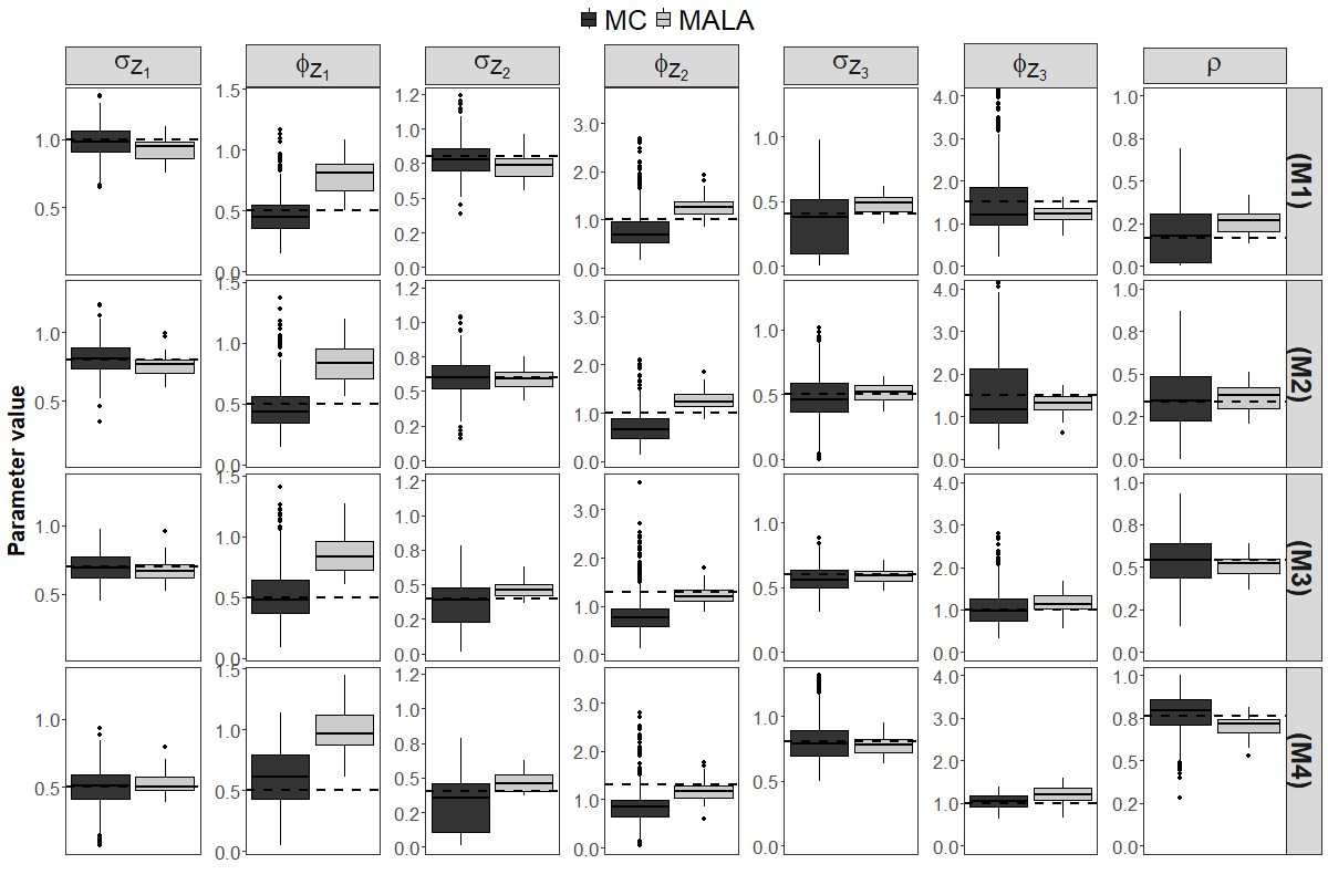
Figure 1: Boxplot of the parameter estimates from MC (colored in dark gray) and MALA using coarse grid (colored in light gray) for positively correlated models (different rows). For MC, we use the optimal control parameters and exclude any estimates that are outside three standard errors of the true parameter values (marked with horizontal lines).

Turning to the results in Figure 1, the MALA estimator performs uniformly well for all models when estimating the scale parameters, $\sigma_{Z_{i}}$ ($i\in\{1,2,3\}$), but not quite as well for the range parameters (e.g., $\phi_{Z_{1}}$). This may indicate the difficulty of obtaining reliable estimators for the range parameters based on the current length of Markov chains ($3.1\times 10^{6}$ iterations). For MC, while the sampling variances of the MC estimators are larger than the corresponding MALA estimators, most of the estimators correctly identify the true parameter values and have nearly symmetric distributions. One exception is on $\phi_{Z_{2}}$. The boxplot of the estimated $\phi_{Z_{2}}$ is underestimated and right-skewed across all models. Some MC estimators, such as $\sigma_{Z_{2}}$ and $\sigma_{Z_{3}}$ in (M3) and $\phi_{Z_{3}}$ in (M4), are competitive to the corresponding MALA estimators.

Bear in mind that the MALA method we use in the simulations is customized for the LGCP model, but the MC method theoretically works for a much wider range of multivariate point process models. Since the data is generated from the LGCP model, MALA has a clear advantage over the MC method. Performance of MC estimators for multivariate point process models not following the LGCP will be investigated in future research.

7 Application: Terrorism in Nigeria

In this section, we apply our methods to the point pattern data of the 2014 terrorism attacks in Nigeria that are considered in Jun and Cook (2022).

The National Consortium for the Study of Terrorism and Responses to Terrorism (START) at the University of Maryland maintains the Global Terrorism Database (GTD; START, 2022). Figure 2 plots the point pattern of terror attacks by Boko Haram (BH; 436 terror attacks) and Fulani Extremists (FE; 156 terror attacks) in Nigeria during 2014.

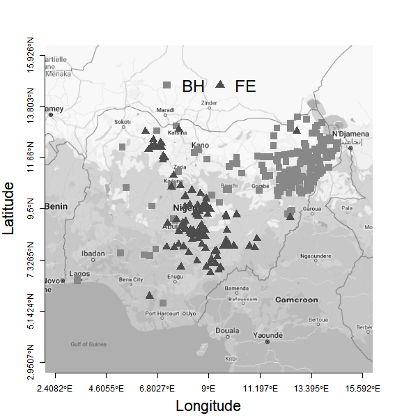
Figure 2: Point pattern of terror attacks by Boko Haram (BH; 436 terror attacks) and Fulani Extremists (FE; 156 terror attacks) in Nigeria during 2014.

In the raw data (which is obtained from the GTD), there are several events with identical spatial coordinates (which occur at different times). Thus, we add a small jittering (added a random Gaussian noise with standard deviation $10^{-3}$ degree (^∘) on both coordinates) to distinguish these events. We observe in Figure 2 that the BH attacks are mostly concentrated on the northeast corner of the country border while the majority of the FE attacks are located in the middle of the country side. This may indicate repulsiveness between the two sources of terror attacks.

To fit the point pattern data, we use the bivariate LGCP model with a negative correlation ($b=-1$) that is considered in Section 6.1. Since our focus is on the second-order marginal and cross-group interactions of BH and FE attacks, we assume that the first-order intensities of the BH and FE are given which are equal to the sample estimators $\widehat{\lambda}_{1}^{(i)}$, $i\in\{BH,FE\}$. Let $\bm{\theta}=(\sigma_{\text{BH}},\phi_{\text{BH}},\sigma_{\text{FE}},\phi_{\text{FE}},\sigma_{\text{Common}},\phi_{\text{Common}})^{\top}$ be the parameter of interest. The indices “BH”, “FE”, and “Common” correspond to $Z_{1}$, $Z_{2}$, and $Z_{3}$ in (6.3), respectivley. We also estimate the cross-correlation coefficient $\rho$ between BH and FE. Using the methods in Section 5.2 (see also, Section 6.2.2), we search for the optimal control parameters over the grids $c\in\{0.1,0.2,0.3,0.4,0.5\}$ and $R\in\{60\text{km},80\text{km},\cdots,500\text{km}\}$ (the sampling window is approximately $1,347\times 1,088$km²), and select the optimal parameter $(c,R)=(0.1,420\text{km})$.

In Table 4, we report the parameter estimation, estimated asymptotic standard error, and two 95% confidence intervals (CI): asymptotic and simulation-based. The asymptotic CI is calculated using the normal approximation of $\widehat{\bm{\theta}}_{n}$ based on Theorem 4.2 (and the Delta method for $\widehat{\rho}$), while the simulation-based CI is derived from the 600 Monte Carlo samples as described in Section 5.1. From the results in Table 4, we observe that both 95% asymptotic and simulation-based CIs suggest no significant difference in the scale ($\sigma_{\text{BH}}$ and $\sigma_{\text{FE}}$) and range ($\phi_{\text{BH}}$ and $\phi_{\text{FE}}$) parameters associated with BH and FE. The appearance of negative values in the lower bound of the asymptotic confidence interval is due to the large standard error. However, both 95% CIs of the cross-correlation coefficient $\widehat{\rho}$ lie on the negative line, suggesting a significant repulsion between BH and FE attacks.

Param.	EST	Asymptotic SE	95% asymptotic CI	95% simulation-based CI
$\sigma_{\text{BH}}$	1.28	0.41	(-0.47, 2.09)	(0.22, 1.58)
$\phi_{\text{BH}}$	63.99	58.04	(-49.77, 177.75)	(5.32, 158.62)
$\sigma_{\text{FE}}$	1.94	0.46	(1.05, 2.83)	(1.15, 2.47)
$\phi_{\text{FE}}$	12.68	24.72	(-35.77, 61.13)	(1.68, 45.48)
$\sigma_{\text{Common}}$	1.33	0.44	(0.48, 2.19)	(0.58, 1.54)
$\phi_{\text{Common}}$	370.43	305.90	(-229.12, 969.99)	(46.46, 400.95)
$\rho$	-0.41	0.17	(-0.74, -0.08)	(-0.62, -0.11)

Table 4: Estimated parameter value (EST), asymptotic standard error (SE), and 95% asymptotic and simulation-based confidence intervals (CI) for the minimum contrast method to fit the terror attacks in Nigeria 2014 by BH and FE. Units of $\phi_{x}$ ($x\in\{\text{BH},\text{FE},\text{Common}\}$) are in kilometers.

To quantify the interactions, using the estimated parameters in Table 4, we calculate the marginal and cross-correlation of BH and FE at distance $r=$ 0km, 50km, 100km, 250km, and 420km. See Equations (E.2)–(E.4) in Appendix for the detailed formulas. The results are summarized in Table 5. These results indicate (1) the BH attacks have a stronger spatial concentration than FE, (2) the strength of the repulsion is weaker than the concentration of BH attacks but stronger than the concentration of FE attacks, and (3) BH and FE still have repulsive behavior at the range of 420km, albeit with a strength that is $1/3$ of that at 0km.

	$r=$0km	$r=$50km	100km	250km	420km
${\mathbb{C}\rm orr}_{\text{BH}}(r;\widehat{\bm{\theta}})$	1	0.67	0.50	0.27	0.17
${\mathbb{C}\rm orr}_{\text{FE}}(r;\widehat{\bm{\theta}})$	1	0.29	0.25	0.16	0.10
${\mathbb{C}\rm orr}_{\text{BH,FE}}(r;\widehat{\bm{\theta}})$	-0.41	-0.36	-0.31	-0.21	-0.13

Table 5: Estimated marginal and cross correlations of BH and FE at different distances.

8 Concluding remarks and discussion

In this article we propose a new inferential method for multivariate stationary spatial point processes. The proposed method is based on minimizing the contrast (MC) between the matrix-valued scaled $K$-function and its nonparametric edge-corrected estimator. When the model is correctly specified, the resulting MC estimator has satisfactory large sample properties. These enable us to conduct a statistical inference of multivariate spatial point processes. Moreover, the proposed method is computationally efficient and the form of the asymptotic covariance matrix of the MC estimator gives an insight into the selection of the optimal control parameters in the discrepancy measure.

From the results in our simulations, we believe that our method may provide a useful alternative to the Bayesian inferential methods when analyzing multivariate spatial point processes. The significantly faster computing time is the chief advantage of our method, making it useful for researchers to obtain the initial values, analyze large samples, and evaluate many models from complicated point processes. Moreover, it is intriguing that for certain parameter settings, our estimator is a close contender of that in Bayesian method. We do not yet have any theoretical basis for the (relative) efficiency of the estimators, but it could be a good avenue for future research.

Lastly, we discuss two possible extensions of our study. Firstly, the emphasis of this paper is on using scaled $K$-function matrix to construct a discrepancy function. However, it is worth considering other second-order measures in the contrast function for certain processes. An example of such an alternative measure is pair correlation functions $G(\bm{x})=[g_{i,j}(\bm{x})]_{i,j=1}^{m}$, where $g_{i,j}(\bm{x})=\lambda_{2,\text{red}}^{(i,j)}(\bm{x})/\{\lambda_{1}^{(i)}\lambda_{1}^{(j)}\}$. A similar argument in Section 4.2 (also, Appendices B and C) can be applied to derive the asymptotic normality of the MC estimator based on the pair correlation function matrix (see,Biscio and Svane (2022), Section 4.1). Secondly, in practical scenarios, the joint stationarity assumption is often considered to be too stringent. Therefore, we may relax this assumption and consider the MC estimator of the second-order intensity reweighted stationary (SOIRS) processes. Indeed, Waagepetersen et al. (2016) proposed a least square estimation of the multivariate SOIRS LGCP process and applied the resulting estimator in clustering analysis. To theoretically justify this extension, the results in Guan (2009) may be useful in this context.

Summary of results in the Supplemental Material

To give direction on how the Supplemental Material (which we will call the Appendix from now on) is organized, we briefly summary the contents of each section.

• In Appendix A, we obtain the first and second moment bounds of the scaled $K$-function estimators under both with or without edge-correction factor. These results are useful to simplify the calculation of an asymptotic covariance matrix of $\widehat{\bm{G}}_{n}(\cdot)$ and also required in the proof of Theorem 4.1.

• In Appendix B, we provide an expression for the asymptotic covariance matrix of $\text{vec}(\widehat{\bm{G}}_{n}(h))$. This is one of the parts of the proof of Theorem 4.1.

• In Appendix C, we prove the results in the main paper.

• In Appendix D, we prove two technical lemmas. The first lemma verifies the Assumption 4.1 for the multivariate LGCPs and the next lemma is required in the proof of Theorem B.1.

• In Appendix E.1, we present explicit form of the covariance structure of the (log of) latent Gaussian random field and the correlation coefficient of the LGCP model that are considered in Section 6.1. In Appendix E.2, we display additional figures and tables that are associated with the simulations in the main paper.

Appendix A A comparison between the two $Q$-function estimators

Let $\{D_{n}\}$ be an increasing sequence of sampling windows of the multivariate stationary point process $\underline{X}=(X_{1},\dots,X_{m})$. Recall (3.2) and (3.3), for $i,j\in\{1,\dots,m\}$, we define the two marginal (if $i=j$) and cross (if $i\neq j$) $Q$-function estimators as:

$$[\widehat{\bm{Q}}_{0n}(r)]_{i,j}=|D_{n}|^{-1}\sum_{\bm{x}\in X_{i}}\sum_{\bm{y}\in X_{j}}\textbf{1}_{\{0<\|\bm{x}-\bm{y}\|\leq r\}}$$ (A.1)

and

$$[\widehat{\bm{Q}}_{n}(r)]_{i,j}=|D_{n}|^{-1}\sum_{\bm{x}\in X_{i}}\sum_{\bm{y}\in X_{j}}b(\bm{x},\bm{y})\textbf{1}_{\{0<\|\bm{x}-\bm{y}\|\leq r\}},\quad r\geq 0\quad\text{and}\quad n\in\mathbb{N},$$ (A.2)

where $b(\cdot,\cdot)$ is an edge-correction factor that belongs to either $b_{1}$, $b_{2}$, or $b_{3}$. We note that if $\underline{X}$ is simple, then, the definition of (A.2) is almost surely equal to the scaled marginal $K$-function (3.3) (when $i=j$) or cross $K$-function (3.6) (when $i\neq j$) for all $i,j\in\{1,\dots,m\}$. The following theorem addresses the first and second moment bounds for $[\widehat{\bm{Q}}_{0n}(r)]_{i,j}$ and $[\widehat{\bm{Q}}_{n}(r)]_{i,j}$. The proof technique is almost identical to that in Biscio and Svane (2022), Theorems 3.5 and 4.1., so we omit the details.

Theorem A.1

Let $\underline{X}=(X_{1},\dots,X_{m})$ be a multivariate stationary point process that satisfies Assumption 4.1(i) (for $\ell=4$). Moreover, we assume that the increasing sequence of sampling windows $\{D_{n}\}$ in $\mathbb{R}^{d}$ is c.a.w. and the edge-correction factor is such that $b\in\{b_{1},b_{2}\}$ (or $b\in\{b_{1},b_{2},b_{3}\}$, assuming $\underline{X}$ is isotropic). Then, for $i,j\in\{1,\dots,m\}$, the following three assertions hold:

$$\mathbb{E}[[\widehat{\bm{Q}}_{0n}(r)]_{i,j}-[\widehat{\bm{Q}}_{n}(r)]_{i,j}]=O(n^{-1}),$$ (A.3)

$${\mathbb{V}\rm ar}\{[\widehat{\bm{Q}}_{0n}(r)]_{i,j}-[\widehat{\bm{Q}}_{n}(r)]_{i,j}\}=O(n^{-1}|D_{n}|^{-1})=O(n^{-d-1}),\quad\text{and}$$ (A.4)

$${\mathbb{V}\rm ar}\{[\widehat{\bm{Q}}_{n}(r)]_{i,j}\}=O(|D_{n}|^{-1})=O(n^{-d}).$$ (A.5)

As a corollary, we show that the asymptotic covariance matrix of $\text{vec}(\widehat{\bm{G}}_{n}(h))$ (defined as in (4.10)) is equal to the asymptotic covariance matrix of a vectorization of non-edge corrected counterparts

$$[\widehat{\bm{G}}_{0n}(h)]_{i,j}=|D_{n}|^{1/2}\left\{[\widehat{\bm{Q}}_{0n}(h)]_{i,j}-\mathbb{E}[\widehat{\bm{Q}}_{0n}(h)]_{i,j}\right\},\quad i,j\in\{1,\dots,m\}\quad\text{and}\quad h\geq 0.$$ (A.6)

Corollary A.1

Suppose the same set of Assumptions and notation as in Theorem A.1 holds. For $i,j\in\{1,\dots,m\}$, let $[\widehat{\bm{G}}_{n}(h)]_{i,j}$ and $[\widehat{\bm{G}}_{0n}(h)]_{i,j}$ are defined as in (4.9) and (A.6), respectively. Then,

$$\lim_{n\rightarrow\infty}\left|{\mathbb{C}\rm ov}\left\{[\widehat{\bm{G}}_{n}(h)]_{a,b},[\widehat{\bm{G}}_{n}(h)]_{c,d}\right\}-{\mathbb{C}\rm ov}\left\{[\widehat{\bm{G}}_{0n}(h)]_{a,b},[\widehat{\bm{G}}_{0n}(h)]_{c,d}\right\}\right|=0,\qquad a,b,c,d\in\{1,\dots,m\}.$$ (A.7)

PROOF. By triangular inequality and Cauchy-Schwarz inequality, we have

$$|{\mathbb{C}\rm ov}(X_{1},Y_{1})-{\mathbb{C}\rm ov}(X_{2},Y_{2})|$$

$$\quad\leq|{\mathbb{C}\rm ov}(X_{1}-X_{2},Y_{1})|+|{\mathbb{C}\rm ov}(X_{2},Y_{1}-Y_{2})|$$

$$\quad\leq\{{\mathbb{V}\rm ar}(X_{1}-X_{2})\}^{1/2}\{{\mathbb{V}\rm ar}(Y_{1})\}^{1/2}+\{{\mathbb{V}\rm ar}(Y_{1}-Y_{2})\}^{1/2}\{{\mathbb{V}\rm ar}(X_{2})\}^{1/2}.$$ (A.8)

Let $X_{1}=[\widehat{\bm{G}}_{n}(h)]_{a,b}$, $X_{2}=[\widehat{\bm{G}}_{0n}(h)]_{a,b}$, $Y_{1}=[\widehat{\bm{G}}_{n}(h)]_{c,d}$, and $Y_{2}=[\widehat{\bm{G}}_{0n}(h)]_{c,d}$. Then, from (A.4), we have

$${\mathbb{V}\rm ar}(X_{1}-X_{2})=|D_{n}|{\mathbb{V}\rm ar}\{[\widehat{\bm{Q}}_{0n}(h)]_{a,b}-[\widehat{\bm{Q}}_{n}(h)]_{a,b}\}=O(n^{-1}),\quad n\rightarrow\infty.$$ (A.9)

Similarly, ${\mathbb{V}\rm ar}(Y_{1}-Y_{2})=O(n^{-1})$ as $n\rightarrow\infty$. Moreover, from (A.4) and (A.5), we have

$${\mathbb{V}\rm ar}X_{2}\leq 2({\mathbb{V}\rm ar}(X_{2}-X_{1})+{\mathbb{V}\rm ar}(X_{1}))=O(1),\quad n\rightarrow\infty.$$ (A.10)

Similarly, we have ${\mathbb{V}\rm ar}Y_{1}=O(1)$ as $n\rightarrow\infty$. Substitute (A.9) and (A.10) into (A.8) gives

$$\left|{\mathbb{C}\rm ov}\{[\widehat{\bm{G}}_{n}(h)]_{a,b},[\widehat{\bm{G}}_{n}(h)]_{c,d}-{\mathbb{C}\rm ov}\{[\widehat{\bm{G}}_{0n}(h)]_{a,b},[\widehat{\bm{G}}_{0n}(h)]_{c,d}\right|=O(n^{-1/2}),\qquad a,b,c,d\in\{1,\dots,m\}$$

as $n\rightarrow\infty$. Thus, we get the desired results. $\Box$

Appendix B Expression for the asymptotic covariance matrix

In this section, we provide an expression for the asymptotic covariance matrix of $\text{vec}(\widehat{\bm{G}}_{n}(h))$ defined as in (4.10) in terms of the joint intensity functions of underlying point process $\underline{X}$. Let

$$\sigma^{2}_{(a,b:c,d)}(h)=\lim_{n\rightarrow\infty}{\mathbb{C}\rm ov}\left\{[\widehat{\bm{G}}_{n}(h)]_{a,b},[\widehat{\bm{G}}_{n}(h)]_{c,d}\right\},\quad a,b,c,d\in\{1,\dots,m\},$$ (B.1)

be the entries of $\Sigma(h;\bm{\theta}_{0})=\lim_{n\rightarrow\infty}{\mathbb{V}\rm ar}\left\{\text{vec}(\widehat{\bm{G}}_{n}(h))\right\}$. Due to the asymmetricity of the edge-correction, $\widehat{\bm{G}}_{n}(h)$ is not symmetric. Therefore, cases to consider in the expression of $\sigma^{2}_{(a,b:c,d)}(h)$ could be very cumbersome. As a remedy, for $i,j\in\{1,\dots,m\}$, let $[\widehat{\bm{Q}}_{0n}(h)]_{i,j}$ be a nonparametric estimator of $[\bm{Q}(h;\bm{\theta}_{0})]_{i,j}$, but without the edge-correction (see, (A.1)). Let

$$\eta^{2}_{(a,b:c,d)}(h)=\lim_{n\rightarrow\infty}{\mathbb{C}\rm ov}\left\{[\widehat{\bm{G}}_{0n}(h)]_{a,b},[\widehat{\bm{G}}_{0n}(h)]_{c,d}\right\},\quad a,b,c,d\in\{1,\dots,m\},$$ (B.2)

where $[\widehat{\bm{G}}_{0n}(h)]_{i,j}$ is an empirical process of $[\bm{Q}(h;\bm{\theta}_{0})]_{i,j}$ defined as in (A.6). Then, in Corollary A.1, we show

$$\sigma^{2}_{(a,b:c,d)}(h)=\eta^{2}_{(a,b:c,d)}(h),\quad a,b,c,d\in\{1,\dots,m\}.$$ (B.3)

One advantage of using $\eta^{2}_{(a,b:c,d)}(h)$ over $\sigma^{2}_{(a,b:c,d)}(h)$ is that $\widehat{\bm{G}}_{0n}(h)$ is symmetric. Therefore, the number of different cases to consider in the expression $\eta^{2}_{(a,b:c,d)}(h)$ has significantly reduced. Below, we provide the complete list of expressions for $\sigma^{2}_{(a,b:c,d)}(h)$.

Theorem B.1

Let $\underline{X}=(X_{1},\dots,X_{m})$ be a multivariate stationary point process that satisfies Assumption 4.1(i) (for $\ell=4$). Moreover, we assume that the increasing sequence of sampling windows $\{D_{n}\}$ in $\mathbb{R}^{d}$ is c.a.w. and the edge-correction factor is such that $b\in\{b_{1},b_{2}\}$ (or $b\in\{b_{1},b_{2},b_{3}\}$, assuming $\underline{X}$ is isotropic). Then, $\sigma^{2}_{(a,b:c,d)}(h)$ is well-defined for all $a,b,c,d\in\{1,\dots,m\}$ and we have

$$\sigma^{2}_{(a,b:c,d)}(h)=\sigma^{2}_{(b,a:c,d)}(h)=\sigma^{2}_{(a,b:d,c)}(h)=\sigma^{2}_{(b,a:d,c)}(h),\quad a,b,c,d\in\{1,\dots,m\}.$$ (B.4)

Let $i,j,k,\ell$ be the distinct indices of $\{1,\dots,m\}$ (If $m<4$, then, we select at most $m$ distinct indices) and $I()$ be the indicator function. Then, using (B.4), we have seven distinct expressions for $\sigma^{2}_{(a,b:c,d)}(h)$, which we will list below.

[case1]: $(a,b)=(c,d)=(i,i)$;

$$\sigma^{2}_{(i,i:i,i)}(h)$$

$$\quad=\iiint I(\|{\bm{u}}_{1}\|\leq h)I(\|{\bm{u}}_{3}\|\leq h)\left\{\lambda^{(i)}_{4,red}({\bm{u}}_{1},{\bm{u}}_{2},{\bm{u}}_{2}+{\bm{u}}_{3})-\lambda^{(i)}_{2,red}({\bm{u}}_{1})\lambda^{(i)}_{2,red}({\bm{u}}_{3})\right\}d{\bm{u}}_{1}d{\bm{u}}_{2}d{\bm{u}}_{3}$$

$$\qquad+4\iint I(\|{\bm{u}}_{1}\|\leq h)I(\|{\bm{u}}_{2}\|\leq h)\lambda^{(i)}_{3,red}({\bm{u}}_{1},{\bm{u}}_{2})d{\bm{u}}_{1}d{\bm{u}}_{2}+2\int I(\|{\bm{u}}_{1}\|\leq h)\lambda^{(i)}_{2,red}({\bm{u}}_{1})d{\bm{u}}_{1}.$$

[case2]: $(a,b)=(c,d)=(i,j)$;

$$\sigma^{2}_{(i,j:i,j)}(h)$$

$$\quad=\iiint I(\|{\bm{u}}_{1}\|\leq h)I(\|{\bm{u}}_{3}\|\leq h)\left\{\lambda^{(i,j)}_{2,2}({\bm{u}}_{2},{\bm{u}}_{1},{\bm{u}}_{2}+{\bm{u}}_{3})-\lambda^{(i,j)}_{1,1,red}({\bm{u}}_{1})\lambda^{(i,j)}_{1,1,red}({\bm{u}}_{3})\right\}d{\bm{u}}_{1}d{\bm{u}}_{2}d{\bm{u}}_{3}$$

$$\qquad+\iint I(\|{\bm{u}}_{1}\|\leq h)I(\|{\bm{u}}_{2}\|\leq h)\left\{\lambda^{(i,j)}_{2,1,red}({\bm{u}}_{1},{\bm{u}}_{1}+{\bm{u}}_{2})+\lambda^{(j,i)}_{1,2,red}({\bm{u}}_{1},{\bm{u}}_{2})\right\}d{\bm{u}}_{1}d{\bm{u}}_{2}$$

$$\qquad+\int I(\|{\bm{u}}_{1}\|\leq h)\lambda^{(i,j)}_{1,1,red}({\bm{u}}_{1})d{\bm{u}}_{1}.$$

[case3]: $(a,b)=(i,i),(c,d)=(j,j)$;

$$\sigma^{2}_{(i,i:j,j)}(h)$$

$$\quad=\iiint I(\|{\bm{u}}_{1}\|\leq h)I(\|{\bm{u}}_{3}\|\leq h)\left\{\lambda^{(i,j)}_{2,2,red}({\bm{u}}_{1},{\bm{u}}_{2},{\bm{u}}_{2}+{\bm{u}}_{3})-\lambda^{(i,j)}_{1,1,red}({\bm{u}}_{1})\lambda^{(i,j)}_{1,1,red}({\bm{u}}_{3})\right\}d{\bm{u}}_{1}d{\bm{u}}_{2}d{\bm{u}}_{3}$$

[case4]: $(a,b)=(i,i),(c,d)=(i,j)$;

$$\sigma^{2}_{(i,i:i,j)}(h)$$

$$\quad=\iiint I(\|{\bm{u}}_{1}\|\leq h)I(\|{\bm{u}}_{3}\|\leq h)\left\{\lambda^{(i,j)}_{3,1,red}({\bm{u}}_{1},{\bm{u}}_{2},{\bm{u}}_{2}+{\bm{u}}_{3})-\lambda^{(i)}_{2,red}({\bm{u}}_{1})\lambda^{(i,j)}_{1,1,red}({\bm{u}}_{3})\right\}d{\bm{u}}_{1}d{\bm{u}}_{2}d{\bm{u}}_{3}$$

$$\qquad+\iint I(\|{\bm{u}}_{1}\|\leq r)I(\|{\bm{u}}_{2}\|\leq h)\left\{\lambda^{(i,j)}_{2,1,red}({\bm{u}}_{1},{\bm{u}}_{1}+{\bm{u}}_{2})+\lambda^{(i,j)}_{2,1,red}({\bm{u}}_{1},{\bm{u}}_{2})\right\}d{\bm{u}}_{1}d{\bm{u}}_{2}.$$

[case5]: $(a,b)=(i,i),(c,d)=(j,k)$;

$$\sigma^{2}_{(i,i:j,k)}(h)$$

$$\quad=\iiint I(\|{\bm{u}}_{1}\|\leq h)I(\|{\bm{u}}_{3}\|\leq h)\left\{\lambda^{(i,j,k)}_{2,1,1,red}({\bm{u}}_{1},{\bm{u}}_{2},{\bm{u}}_{2}+{\bm{u}}_{3})-\lambda^{(i)}_{2,red}({\bm{u}}_{1})\lambda^{(j,k)}_{1,1,red}({\bm{u}}_{3})\right\}d{\bm{u}}_{1}d{\bm{u}}_{2}d{\bm{u}}_{3}$$

[case6]: $(a,b)=(i,j),(c,d)=(i,k)$;

$$\sigma^{2}_{(i,j:i,k)}(h)$$

$$\quad=\iiint I(\|{\bm{u}}_{1}\|\leq h)I(\|{\bm{u}}_{3}\|\leq h)\left\{\lambda^{\{i,j,k\}}_{2,1,1,red}({\bm{u}}_{2},{\bm{u}}_{1},{\bm{u}}_{2}+{\bm{u}}_{3})-\lambda^{(i,j)}_{1,1,red}({\bm{u}}_{1})\lambda^{(i,k)}_{1,1,red}({\bm{u}}_{3})\right\}d{\bm{u}}_{1}d{\bm{u}}_{2}d{\bm{u}}_{3}$$

$$\qquad+\iint I(\|{\bm{u}}_{1}\|\leq h)I(\|{\bm{u}}_{2}\|\leq h)\lambda^{(i,j,k)}_{1,1,1,red}({\bm{u}}_{1},{\bm{u}}_{2})d{\bm{u}}_{1}d{\bm{u}}_{2}.$$

[case7]: $(a,b)=(i,j),(c,d)=(k,\ell)$;

$$\sigma^{2}_{(i,j:i,k)}(h)$$

$$\quad=\iiint I(\|{\bm{u}}_{1}\|\leq h)I(\|{\bm{u}}_{3}\|\leq h)\left\{\lambda^{(i,j,k,\ell)}_{1,1,1,1,red}({\bm{u}}_{1},{\bm{u}}_{2},{\bm{u}}_{2}+{\bm{u}}_{3})-\lambda^{(i,j)}_{1,1}({\bm{u}}_{1})\lambda^{(k,\ell)}_{1,1,red}({\bm{u}}_{3})\right\}d{\bm{u}}_{1}d{\bm{u}}_{2}d{\bm{u}}_{3}.$$

PROOF. Under (4.2) and Assumption 4.1, for $i,j\in\{1,\dots,m\}$, it is straightforward that the limit of ${\mathbb{V}\rm ar}[\widehat{\bm{G}}_{n}(h)]_{i,j}$ finitely exist. Then, using the identity:

$${\mathbb{C}\rm ov}(X,Y)=\frac{1}{2}\left({\mathbb{V}\rm ar}\{X+Y\}-{\mathbb{V}\rm ar}X-{\mathbb{V}\rm ar}Y\right),$$

$\sigma^{2}_{(a,b:c,d)}(h)$ also exists for all $a,b,c,d\in\{1,\dots,m\}$. Showing (B.4) is a direct consequence of (B.3) and the symmetricity of $\widehat{\bm{G}}_{0n}(h)$.

Next, we calculate the expression for $\eta^{2}_{(a,b:c,d)}(h)$ which is equal to $\sigma^{2}_{(a,b:c,d)}(h)$ due to (B.3). An expression for $\eta^{2}_{(a,b:c,d)}(h)$ varies with the number of overlapping indices in $a,b,c,d$, thus we separate into seven cases as mentioned in the Thoerem. Since [case 1] is shown in Guan and Sherman (2007), Appendix B, we show [case 2]; and [case 3]–[case 6] can be derived in the same way. Let $\phi(\bm{x},\bm{y})=I(0<\|\bm{x}-\bm{y}\|\leq h)$, and simplify the notation $\bm{x}\in X_{i}$ to $\bm{x}\in[i]$ for $i\in\{1,\dots,m\}$. Using (B.1) and (A.1), for $i\neq j$, we have

$${\mathbb{C}\rm ov}\left\{[\widehat{\bm{G}}_{0n}(h)]_{i,j},[\widehat{\bm{G}}_{0n}(h)]_{i,j}\right\} = |D_{n}|^{-1}{\mathbb{C}\rm ov}\left\{\sum_{\bm{x}\in[i],\bm{y}\in[j]}\phi(\bm{x},\bm{y}),\sum_{\bm{z}\in[i],\bm{w}\in[j]}\phi(\bm{z},\bm{w})\right\}$$

$$= |D_{n}|^{-1}\mathbb{E}\left[\sum_{\bm{x},\bm{z}\in[i];~{}\bm{y},\bm{w}\in[j]}\phi(\bm{x},\bm{y})\phi(\bm{z},\bm{w})\right]$$

$$-|D_{n}|^{-1}\mathbb{E}\left[\sum_{\bm{x}\in[i],~{}\bm{y}\in[j]}\phi(\bm{x},\bm{y})]\right]\mathbb{E}\left[\sum_{\bm{z}\in[i],~{}\bm{w}\in[j]}\phi(\bm{z},\bm{w})\right].$$

Since $\underline{X}$ is simple, $P\left(\bm{x}\in[i]~{}~{}\&~{}~{}\bm{x}\in[j]\right)=0$. Therefore, the above can be decomposed as

$${\mathbb{C}\rm ov}\left\{[\widehat{\bm{G}}_{0n}(h)]_{i,j},[\widehat{\bm{G}}_{0n}(h)]_{i,j}\right\}=A_{1}+A_{2}+A_{3}+A_{4},$$ (B.5)

where

$$A_{1}=|D_{n}|^{-1}\mathbb{E}\left[\sum_{\bm{x}\in[i],\bm{y}\in[j]}\phi(\bm{x},\bm{y})^{2}\right],\quad A_{2}=|D_{n}|^{-1}\mathbb{E}\left[\sum_{\bm{x}\neq\bm{z}\in[i],\bm{y}\in[j]}\phi(\bm{x},\bm{y})\phi(\bm{z},\bm{y})\right],$$

$$A_{3}=|D_{n}|^{-1}\mathbb{E}\left[\sum_{\bm{x}\in[i],\bm{y}\neq\bm{w}\in[j]}\phi(\bm{x},\bm{y})\phi(\bm{x},\bm{w})\right],\quad\text{and}$$

$$A_{4}=|D_{n}|^{-1}\left\{\mathbb{E}\left[\sum_{\bm{x}\neq\bm{z}\in[i],\bm{y}\neq\bm{w}\in[j]}\phi(\bm{x},\bm{y})\phi(\bm{z},\bm{w})\right]-\mathbb{E}\left[\sum_{\bm{x}\in[i],~{}\bm{y}\in[j]}\phi(\bm{x},\bm{y})]\right]\mathbb{E}\left[\sum_{\bm{z}\in[i],~{}\bm{w}\in[j]}\phi(\bm{z},\bm{w})\right]\right\}.$$

To represent each term above in integral from, we use the celebrated Campbell’s formula (Kallenberg, 1975; Stoyan et al., 2013). That is, for any non-negative measurable function $g:D^{n}\mapsto\mathbb{R}$ ($n\in\mathbb{N}$), we have

$$\mathbb{E}\left[\sum_{\bm{x}_{1},\cdots,\bm{x}_{n}\in X}^{\neq}g(\bm{x}_{1},\cdots,\bm{x}_{n})\right]=\int_{D^{n}}g(\bm{x}_{1},\cdots,\bm{x}_{n})\lambda_{n}(\bm{x}_{1},\cdots,\bm{x}_{n})\mu(d\bm{x}_{1})\cdots\mu(d\bm{x}_{n})$$ (B.6)

where $\sum_{\bm{x}_{1},\cdots,\bm{x}_{n}\in X}^{\neq}$ is the sum over the $n$ pairwise distinct points $\bm{x}_{1},\cdots,\bm{x}_{n}$ in $X$ and $\mu(\cdot)$ is the $d$-dimensional Lebesgue measure. Similarly to (B.6), the joint intensity function $\lambda_{\underline{n}}(\underline{\bm{x}})$ defined as in (2.3) satisfies the following integral representation:

$$\mathbb{E}\left[\sum_{\bm{x}_{1,1},\dots,\bm{x}_{1,n_{1}}\in X_{1}}^{\neq}\cdots\sum_{\bm{x}_{m,1},\dots,\bm{x}_{m,n_{m}}\in X_{m}}^{\neq}g(\underline{\bm{x}})\right]=\int_{D^{N}}g(\underline{\bm{x}})\lambda_{\underline{n}}(\underline{\bm{x}})\mu(d\underline{\bm{x}})$$ (B.7)

for any non-negative measurable function $g:D^{N}\mapsto\mathbb{R}$, where $\mu(d\underline{\bm{x}})=\prod_{i=1}^{m}\prod_{j=1}^{n_{i}}\mu(d\bm{x}_{i,j})$.

Using (B.7) and since $\phi(\bm{x},\bm{y})^{2}=\phi(\bm{x},\bm{y})=I(0<\|\bm{x}-\bm{y}\|\leq h)$, $A_{1}$ can be written as

$$A_{1}=|D_{n}|^{-1}\mathbb{E}\left[\sum_{\bm{x}\in[i],\bm{y}\in[j]}\phi(\bm{x},\bm{y})^{2}\right]=|D_{n}|^{-1}\iint_{D_{n}^{2}}I(0<\|\bm{x}-\bm{y}\|\leq h)\lambda^{(i,j)}_{1,1}(\bm{x},\bm{y})d\bm{x}d\bm{y}.$$

Using change of variables: ${\bm{u}}_{1}=\bm{y}-\bm{x}$ and ${\bm{u}}_{2}=\bm{x}$ and $\lambda^{(i,j)}_{1,1}(\bm{x},\bm{y})=\lambda^{(i,j)}_{1,1,red}(\bm{y}-\bm{x})$ due to stationarity, we have

$$A_{1} = |D_{n}|^{-1}\int_{D_{n}}\left(\int_{D_{n}-{\bm{u}}_{2}}I(0<\|{\bm{u}}_{1}\|\leq h)\lambda^{(i,j)}_{1,1,red}({\bm{u}}_{1})d{\bm{u}}_{1}\right)d{\bm{u}}_{2}$$

$$= |D_{n}|^{-1}\int_{D_{0n}}(\sim)d{\bm{u}}_{2}+|D_{n}|^{-1}\int_{E_{n}}(\sim)d{\bm{u}}_{2},$$

where $D_{n}-{\bm{u}}_{2}=\{{\bm{u}}_{1}-{\bm{u}}_{2}:{\bm{u}}_{1}\in D_{n}\}$, $D_{0n}$ is an inner window of $D_{n}$ of depth $h$ (see, (3.4)), and $E_{n}=D_{0n}^{\text{c}}\cap D_{n}$. We note that since $\underline{X}$ is simple, we have $N_{X_{i}}(\bm{x})N_{X_{j}}(\bm{x})=0$ for all $\bm{x}\in\mathbb{R}^{d}$. Therefore, by definitions (2.6) and (2.5), we have $\lambda^{(i,j)}_{1,1,red}(\textbf{0})=0$. Thus, we can replace $I(0<\|\bm{x}-\bm{y}\|\leq h)$ with $I(\|\bm{x}-\bm{y}\|\leq h)$ in the above equation which makes the formula more concise.

Now, we calculate each terms in $A_{1}$. When ${\bm{u}}_{2}\in D_{0n}$, then $B_{d}({\bm{u}}_{2},h)\subset D_{n}$. Thus,

$$\int_{D_{n}-{\bm{u}}_{2}}I(\|{\bm{u}}_{1}\|\leq h)\lambda^{(i,j)}_{1,1,red}({\bm{u}}_{1})d{\bm{u}}_{1}=\int_{\mathbb{R}^{d}}I(\|{\bm{u}}_{1}\|\leq h)\lambda^{(i,j)}_{1,1,red}({\bm{u}}_{1})d{\bm{u}}_{1}.$$

Therefore, the first integral in $A_{1}$ is

$$|D_{n}|^{-1}\int_{D_{0n}}\int_{D_{n}-{\bm{u}}_{2}}I(\|{\bm{u}}_{1}\|\leq h)\lambda^{(i,j)}_{1,1,red}({\bm{u}}_{1})d{\bm{u}}_{1}d{\bm{u}}_{2}$$

$$\quad=\frac{|D_{0n}|}{|D_{n}|}\int I(\|{\bm{u}}_{1}\|\leq h)\lambda^{(i,j)}_{1,1,red}({\bm{u}}_{1})d{\bm{u}}_{1}.$$ (B.8)

The second integral in $A_{2}$ is bounded with

$$|D_{n}|^{-1}\left|\int_{E_{n}}\int_{D_{n}-{\bm{u}}_{2}}I(\|{\bm{u}}_{1}\|\leq h)\lambda^{(i,j)}_{1,1,red}({\bm{u}}_{1})d{\bm{u}}_{1}d{\bm{u}}_{2}\right|$$

$$\quad\leq|D_{n}|^{-1}\sup_{\|{\bm{u}}\|\leq h}|\lambda^{(i,j)}_{1,1,red}({\bm{u}})|\int_{E_{n}}\int I(\|{\bm{u}}_{1}\|\leq h){\bm{u}}_{1}{\bm{u}}_{2}=O\left(h^{d}\frac{|E_{n}|}{|D_{n}|}\right)=O(n^{-1})$$ (B.9)

as $n\rightarrow\infty$, where the bound for $\sup_{\|{\bm{u}}\|\leq h}|\lambda^{(i,j)}_{1,1,red}({\bm{u}})|$ is due to Assumption 4.1(i) and the last bound is due to (4.2). Combining (B.8), (B.9), and using that $\lim_{n\rightarrow\infty}|D_{0n}|/|D_{n}|=1$ due to (4.2), we have

$$\lim_{n\rightarrow\infty}A_{1}=\int I(\|{\bm{u}}_{1}\|\leq h)\lambda^{(i,j)}_{1,1,red}({\bm{u}}_{1})d{\bm{u}}_{1}.$$

Similarly, we can show

$$\lim_{n\rightarrow\infty}A_{2} = \iint I(\|{\bm{u}}_{1}\|\leq h)I(\|{\bm{u}}_{2}\|\leq h)\lambda^{(i,j)}_{2,1,red}({\bm{u}}_{1},{\bm{u}}_{1}+{\bm{u}}_{2})d{\bm{u}}_{1}d{\bm{u}}_{2}\quad\text{and}$$

$$\lim_{n\rightarrow\infty}A_{3} = \iint I(\|{\bm{u}}_{1}\|\leq h)I(\|{\bm{u}}_{2}\|\leq h)\lambda^{(i,j)}_{1,2,red}({\bm{u}}_{1},{\bm{u}}_{2})d{\bm{u}}_{1}d{\bm{u}}_{2}.$$

Evalulation of $A_{4}$ is slightly different from those in $A_{1}\sim A_{3}$. Again, from Campbell’s formula, we have

$$A_{4} = |D_{n}|^{-1}\iiiint_{D_{n}^{4}}I(\|\bm{x}-\bm{y}\|\leq h)I(\|\bm{z}-\bm{w}\|\leq h)$$

$$\qquad\qquad\times\left\{\lambda^{(i,j)}_{2,2}(\bm{x},\bm{z},\bm{y},\bm{w})-\lambda^{(i,j)}_{1,1}(\bm{x},\bm{y})\lambda^{(i,j)}_{1,1}(\bm{z},\bm{w})\right\}d\bm{x}d\bm{y}d\bm{z}d\bm{w}.$$

By using the following change of variables:

$${\bm{u}}_{1}=\bm{y}-\bm{x},\quad{\bm{u}}_{2}=\bm{z}-\bm{x},\quad{\bm{u}}_{3}=\bm{w}-\bm{z},\quad\text{and}\quad{\bm{u}}_{4}=\bm{x},$$

we have,

$$A_{4}=|D_{n}|^{-1}\int_{D_{n}}\int_{D_{n}-D_{n}}\int_{D_{n}-{\bm{u}}_{4}}I(\|{\bm{u}}_{1}\|\leq h)I(\|{\bm{u}}_{3}\|\leq h)$$

$$\qquad\times\left(\int_{D_{n}-{\bm{u}}_{3}-{\bm{u}}_{4}}\left\{\lambda^{(i,j)}_{2,2,red}({\bm{u}}_{2},{\bm{u}}_{1},{\bm{u}}_{2}+{\bm{u}}_{3})-\lambda^{(i,j)}_{1,1,red}({\bm{u}}_{1})\lambda^{(i,j)}_{1,1,red}({\bm{u}}_{3})\right\}d{\bm{u}}_{2}\right)d{\bm{u}}_{1}d{\bm{u}}_{3}d{\bm{u}}_{4}.$$

It is not straightforward that the above integral exist. However, in Lemma D.2, we show that $\lambda^{(i,j)}_{2,2,red}({\bm{u}}_{2},{\bm{u}}_{1},{\bm{u}}_{2}+{\bm{u}}_{3})-\lambda^{(i,j)}_{1,1,red}({\bm{u}}_{1})\lambda^{(i,j)}_{1,1,red}({\bm{u}}_{3})$ can be written as a sum of the reduced joint cumulant intensities where each term contains ${\bm{u}}_{2}$. Then, the absolutely integrability of the above integral followed since Assumption 4.1(i)(for $\ell=4$). Therefore, we can apply for Fubini’s theorem. Using the similar techniques applied for the representation of $A_{1}$, we can show that

$$\lim_{n\rightarrow\infty}A_{4}=\iiint I(\|{\bm{u}}_{1}\|\leq h)I(\|{\bm{u}}_{3}\|\leq h)$$

$$\qquad\qquad\qquad\times\left\{\lambda^{(i,j)}_{2,2,red}({\bm{u}}_{2},{\bm{u}}_{1},{\bm{u}}_{2}+{\bm{u}}_{3})-\lambda^{(i,j)}_{1,1,red}({\bm{u}}_{1})\lambda^{(i,j)}_{1,1,red}({\bm{u}}_{3})\right\}d{\bm{u}}_{2}d{\bm{u}}_{1}d{\bm{u}}_{3}.$$

All together with (B.5), we prove [case 2]. Thus, proves the theorem. $\Box$

Appendix C Proof of Theorems 4.1 and 4.2

C.1 Proof of Theorem 4.1

We first show (4.11). Since $\underline{X}$ is simple, recall (3.10), for $i,j\in\{1,\dots,m\}$, we have

$$[\widehat{\bm{Q}}_{n}(h)]_{i,j}=\frac{1}{|D_{n}|}\sum_{\bm{x}\in X_{i},\bm{y}\in X_{j}}b(\bm{x},\bm{y})\textbf{1}_{\{0<\|\bm{x}-\bm{y}\|\leq r\}}\quad\text{almost surely for}\quad h\geq 0.$$ (C.1)

Under ergodicity of $\underline{X}$, we can apply Nguyen and Zessin (1976), Theorem 1 (see also, Nguyen and Zessin (1979) and Heinrich (1992)) and obtain

$$[\widehat{\bm{Q}}_{n}(h)]_{i,j}\rightarrow\mathbb{E}[\widehat{\bm{Q}}_{n}(h)]_{i,j}=[\bm{Q}(h;\bm{\theta}_{0})]_{i,j}\quad\text{almost surely for}\quad i,j\in\{1,\dots,m\},~{}~{}h\geq 0.$$

The equality above is due to unbiasedness of $[\widehat{\bm{Q}}_{n}(h)]_{i,j}$ when using the edge-correction factor $b\in\{b_{1},b_{2}\}$ (or $b\in\{b_{1},b_{2},b_{3}\}$, provided that $\underline{X}$ is isotropic). Since both $\widehat{\bm{Q}}_{n}(h)$ and $[\bm{Q}(h;\bm{\theta}_{0})]_{i,j}$ are positive and increasing function of $h\in[0,\infty)$, the uniform almost sure convergence of above on $h\in[0,R]$ can be obtained by applying a standard technique to prove the uniform almost sure convergence of empirical distribution (e.g., Kallenberg (2021), Proposition 5.24). Thus, (4.11) follows.

Next, we show (4.12). Techniques to use to prove (4.12) is similar to the proof of Guan et al. (2004), Theorem 1 and Pawlas (2009), Section 3, so we only sketch the proof. Recall

$$[\widehat{\bm{G}}_{n}(h)]_{i,j}=|D_{n}|^{1/2}\left\{[\widehat{\bm{Q}}_{n}(h)]_{i,j}-[\bm{Q}(h;\bm{\theta}_{0})]_{i,j}\right\},\quad i,j\in\{1,\dots,m\}\quad\text{and}\quad h\geq 0$$

and $\text{vec}(\widehat{\bm{G}}_{n}(h))=([\widehat{\bm{G}}_{n}(h)]_{i,j})_{1\leq i,j\leq m}$ is the $m^{2}$-dimensional vectorization of $\widehat{\bm{G}}_{n}(h)$. To show the central limit theorem of $\text{vec}(\widehat{\bm{G}}_{n}(h))$, we use so-called the sub-block technique. Let $\{D_{\ell(n)}^{i}:1\leq i\leq k_{n}\}$ be the $k_{n}$ number of non-overlapping subcubes of $D_{n}$ with side length $\ell(n)=n^{\beta}$, where

$$\beta\in(2d/(2d+\varepsilon),1),$$ (C.2)

where $\varepsilon>0$ is from Assumption 4.1(ii). Since $\{D_{\ell(n)}^{i}:1\leq i\leq k_{n}\}$ are non-overlapping, we have

$$\left|\cup_{i=1}^{k_{n}}D_{\ell(n)}^{i}\right|=k_{n}\ell(n)^{d}=k_{n}n^{d\beta}\leq|D_{n}|\leq Cn^{d},$$

where the last inequality is due to (4.2). Therefore, we have

$$k_{n}=O(n^{d(1-\beta)})\quad\text{as}\quad n\rightarrow\infty.$$ (C.3)

Next, let $\{D_{m(n)}^{i}:1\leq i\leq k_{n}\}$ be the subcubes of $\{D_{\ell(n)}^{i}:1\leq i\leq k_{n}\}$, where for $i\in\{1,\dots,k_{n}\}$, $D_{m(n)}^{i}$ is a subcube of $D_{\ell(n)}^{i}$ with the same center and side length

$$m(n)=n^{\beta}-n^{\eta}<n^{\beta}=\ell(n)\quad\text{for some}\quad\eta\in(2d/(2d+\varepsilon),\beta).$$ (C.4)

Then, we have

$$d(D_{\ell(n)}^{i},D_{m(n)}^{j})\leq n^{\eta}\quad\text{for}\quad i\neq j\in\{1,\dots,k_{n}\}.$$ (C.5)

For $i\in\{1,\dots,k_{n}\}$, let $\widehat{\bm{Q}}_{n}^{(i)}(h)$, $h\geq 0$, be a nonparametric edge-corrected estimator of $\bm{Q}(h;\bm{\theta}_{0})$ defined similarly to (3.10), but within the sampling window $D_{m(n)}^{i}$. For $i\in\{1,\dots,k_{n}\}$, let

$$[\widehat{\bm{G}}_{n}^{(i)}(h)]_{p,q}=|D_{m(n)}^{i}|^{1/2}\left\{[\widehat{\bm{Q}}_{n}^{(i)}(h)]_{p,q}-[\bm{Q}(h;\bm{\theta}_{0})]_{p,q}\right\},\quad p,q\in\{1,\dots,m\}\quad\text{and}\quad h\geq 0$$ (C.6)

and

$$[T_{n}]_{p,q}=k_{n}^{-1/2}\sum_{i=1}^{k_{n}}[\widehat{\bm{G}}_{n}^{(i)}(h)]_{p,q}\quad\text{and}\quad[\widetilde{T}_{n}]_{p,q}=k_{n}^{-1/2}\sum_{i=1}^{k_{n}}[\widetilde{\bm{G}}_{n}^{(i)}(h)]_{p,q},\quad p,q\in\{1,\dots,m\},$$ (C.7)

where for $i\in\{1,\dots,k_{n}\}$, $[\widetilde{\bm{G}}_{n}^{(i)}(h)]_{p,q}$ is an independent copy of $[\widehat{\bm{G}}_{n}^{(i)}(h)]_{p,q}$.

Let $\text{vec}(T_{n})=([T_{n}]_{p,q})_{1\leq p,q\leq m}$ be the vectorization of $\{[T_{n}]_{p,q}\}$ and $\text{vec}(\widetilde{T}_{n})$ is defined similarly but replacing $[T_{n}]_{p,q}$ with $[\widetilde{T}_{n}]_{p,q}$. Our goal is to show $\text{vec}(\widehat{\bm{G}}_{n}(h))$ and $\text{vec}(\widetilde{T}_{n})$ are asymptotically negligible, thus, they have the same asymptotic distribution. To prove this, we use an intermediate random variable, $\text{vec}(T_{n})$. We first show

$$\text{vec}(\widehat{\bm{G}}_{n}(h))-\text{vec}(T_{n})\stackrel{{\scriptstyle\mathcal{P}}}{{\rightarrow}}0.$$ (C.8)

To show this, we bound the first and second moment of the difference. Since $\mathbb{E}[\text{vec}(\widehat{\bm{G}}_{n}(h))]=\mathbb{E}[\text{vec}(T_{n})]=\textbf{0}_{m\times m}$, the first moment of the difference is zero. To bound the second moment, we will show

$${\mathbb{V}\rm ar}\left\{[\widehat{\bm{G}}_{n}(h)]_{p,q}-[T_{n}]_{p,q}\right\}\rightarrow 0\quad\text{as }n\rightarrow\infty\quad\text{for}\quad p,q\in\{1,\dots,m\},$$ (C.9)

then, by Markov’s inequality, we can prove (C.8). To show (C.9), let $[\widehat{\bm{G}}_{0n}(h)]_{p,q}$ defined as in (A.6) be the empirical process of the $\bm{Q}(h;\bm{\theta}_{0})$ without edge-correction. Similarly, we define $[\widehat{\bm{G}}_{0n}^{(i)}(h)]_{p,q}$ and $[T_{0n}]_{p,q}$ as an analogous no-edge-corrected estimators to (C.6) and (C.7), respectively. Then, by Cauchy-Schwarz inequality, we have

$${\mathbb{V}\rm ar}\left\{[\widehat{\bm{G}}_{n}(h)]_{p,q}-[T_{n}]_{p,q}\right\} \leq 3\bigg{(}{\mathbb{V}\rm ar}\left\{[\widehat{\bm{G}}_{n}(h)]_{p,q}-[\widehat{\bm{G}}_{0n}(h)]_{p,q}\right\}+{\mathbb{V}\rm ar}\left\{[\widehat{\bm{G}}_{0n}(h)]_{p,q}-[T_{0n}]_{p,q}\right\}$$

$$\quad+{\mathbb{V}\rm ar}\left\{[T_{0n}]_{p,q}-[T_{n}]_{p,q}\right\}\bigg{)},\qquad p,q\in\{1,\dots,m\}.$$

By Lemma A.1, the first and third term above is of order $O(n^{-1})$. The second term converges to zero as $n\rightarrow\infty$, due to the calculations in Pawlas (2009), page 4200 (we omit the detail). Therefore, all together, we show (C.9) and thus, (C.8) holds.

Next, we will show

$$\text{vec}(T_{n})-\text{vec}(\widetilde{T}_{n})\stackrel{{\scriptstyle\mathcal{D}}}{{\rightarrow}}0.$$ (C.10)

To show this, we focus on the characteristic function of $\text{vec}(T_{n})$ and $\text{vec}(\widetilde{T}_{n})$. For $n\in\mathbb{N}$, let $\phi_{n}(\underline{t})$ and $\widetilde{\phi}_{n}(\underline{t})$ are the characteristic function of $\text{vec}(T_{n})$ and $\text{vec}(\widetilde{T}_{n})$, respectively, where $\underline{t}\in\mathbb{R}^{m^{2}}$. To show (C.10), it is enough to show

$$|\phi_{n}(\underline{t})-\widetilde{\phi}_{n}(\underline{t})|\rightarrow 0\quad\text{as }n\rightarrow\infty\quad\text{for all}\quad t\in\mathbb{R}^{m^{2}}.$$ (C.11)

Proof of (C.11) is standard method using telescoping sum. Let

$$U_{n}^{(i)}=\exp\left(i\frac{\langle\underline{t},\text{vec}(\widehat{\bm{G}}_{n}^{(i)})\rangle}{k_{n}^{1/2}}\right),\quad i\in\{1,\dots,k_{n}\},$$

where $\langle\cdot,\cdot\rangle$ is the dot product and $\text{vec}(\widehat{\bm{G}}_{n}^{(i)})$ is the vectorization of $[\widehat{\bm{G}}_{n}^{(i)}(h)]_{p,q}$. Similarly for $i\in\{1,\dots,k_{n}\}$, we can define $\widetilde{U}_{n}^{(i)}$ by replacing $[\widehat{\bm{G}}_{n}^{(i)}(h)]_{p,q}$ with $[\widetilde{\bm{G}}_{n}^{(i)}(h)]_{p,q}$ in the above definition. Then, by definition,

$$\phi_{n}(\underline{t})=\mathbb{E}\left[\prod_{i=1}^{k_{n}}U_{n}^{(i)}\right]\quad\text{and}\quad\widetilde{\phi}_{n}(\underline{t})=\mathbb{E}\left[\prod_{i=1}^{k_{n}}\widetilde{U}_{n}^{(i)}\right].$$

Since $\widetilde{U}_{n}^{(i)}$ are jointly independent and has the same marginal distribution with $U_{n}^{(i)}$, we have $\widetilde{\phi}_{n}(\underline{t})=\prod_{i=1}^{k_{n}}\mathbb{E}\widetilde{U}_{n}^{(i)}=\prod_{i=1}^{k_{n}}\mathbb{E}U_{n}^{(i)}$. Therefore, using telescoping sum argument (cf. Pawlas (2009), equation (13)), we have

$$|\phi_{n}(\underline{t})-\widetilde{\phi}_{n}(\underline{t})|\leq\sum_{j=1}^{k_{n}-1}\left|{\mathbb{C}\rm ov}\left\{\prod_{i=1}^{j}U_{n}^{(i)},U_{n}^{(j+1)}\right\}\right|.$$ (C.12)

Now, we use the $\alpha$-mixing condition. We first note that

$$\text{vec}(\widehat{\bm{G}}_{n}^{(i)})\in(\mathcal{F}(D_{m(n)}^{i}))^{m^{2}},\quad i\in\{1,\dots,k_{n}\},$$

where for $E\in\mathbb{R}^{d}$, $\mathcal{F}(E)$ is the sigma algebra generated by $\underline{X}$ in the sampling window $E$. Therefore, for $j\in\{1,\dots,k_{n}-1\}$

$$\prod_{i=1}^{j}U_{n}^{(i)}\in\mathcal{F}(\cup_{i=1}^{j}D_{m(n)}^{i})\quad\text{and}\quad U_{n}^{(j+1)}\in\mathcal{F}(D_{m(n)}^{j+1}).$$

We note that

$$|U_{j}|\leq 1,\quad|D_{m(n)}^{j+1}|\leq|\cup_{i=1}^{j}D_{m(n)}^{i}|=jm(n)^{d},\quad\text{and}\quad d\left(\cup_{i=1}^{j}D_{m(n)}^{i},D_{m(n)}^{j+1}\right)\leq n^{\eta},\qquad j\in\{1,\dots,k_{n}-1\},$$

where the last inequality is due to (C.5). Therefore, using the $\alpha$-mixing coefficient defined as in (4.3) and the strong-mixing inequality (cf. Pawlas (2009), equation (9)), we have

$$\left|{\mathbb{C}\rm ov}\left\{\prod_{i=1}^{j}U_{n}^{(i)},U_{n}^{(j+1)}\right\}\right|\leq 4\alpha_{jm(n)^{d}}(n^{\eta})\leq Cjm(n)^{d}n^{-\eta(d+\varepsilon)},\qquad j\in\{1,\dots,k_{n}-1\},$$

where the last inequality is due to 4.1(ii). Summing the above over $j$ and using the bounds (C.3) and (C.4), we have,

$$|\phi_{n}(\underline{t})-\widetilde{\phi}_{n}(\underline{t})|\leq 4\sum_{j=1}^{k_{n}-1}jm(n)^{d}n^{-\eta(d+\varepsilon)}\leq Ck_{n}^{2}m(n)^{d}n^{-\eta(d+\varepsilon)}=O(n^{2d-\beta d-\eta(d+\varepsilon)}).$$ (C.13)

Since $\eta\in(2d/(2d+\varepsilon),\beta)$, we have for all $t\in\mathbb{R}^{m^{2}}$, $|\phi_{n}(\underline{t})-\widetilde{\phi}_{n}(\underline{t})|\rightarrow 0$ as $n\rightarrow\infty$. Therefore, we show (C.11), thus, (C.10).

Back to our goal, combing (C.8) and (C.10), $\text{vec}(\widehat{\bm{G}}_{n}(h))$ and $\text{vec}(\widetilde{T}_{n})$ shares the same asymptotic distribution. Now, we find the asymptotic distribution of $\text{vec}(\widetilde{T}_{n})$. Recall, (C.7),

$$\text{vec}(\widetilde{T}_{n})=k_{n}^{-1/2}\sum_{i=1}^{k_{n}}\text{vec}(\widetilde{\bm{G}}_{n}^{(i)}(h))$$

and $\{\text{vec}(\widetilde{\bm{G}}_{n}^{(i)}(h))\}$ are i.i.d. mean zero random vectors. Since $\{D_{n}\}$ is c.a.w., we can let $k_{n}\rightarrow\infty$. Therefore, under (4.6), we can apply for Lyapunov CLT to conclude $\text{vec}(\widetilde{T}_{n})$ converges to the centered normal distribution. To calculate the asymptotic covariance matrix of $\{\text{vec}(\widetilde{\bm{G}}_{n}^{(1)}(h))\}$ , since $\{D_{m(n)}^{1}\}$ satisfies (4.2), the asymptotic covariance matrix of $\{\text{vec}(\widetilde{\bm{G}}_{n}^{(1)}(h))\}$ is the same as the asymptotic covariance matrix of $\text{vec}(\widetilde{\bm{G}}_{n}(h))$, where the exact expression can be found in Appendix B. $\Box$

C.2 Proof of Theorem 4.2

The proof technique is similar to the techniques developed in Guan and Sherman (2007), Appendix C.

First, we will show $\widehat{\bm{\theta}}_{n}$, the minimizer of $U_{n}(\bm{\theta})$, exists for all $n\in\mathbb{N}$. To show this, since $\Theta$ is compact, from the expression (3.12), it is enough to show for all $i,j\in\{1,\dots,m\}$,

$$\int_{0}^{R}[\bm{Q}(h;\bm{\theta})]_{i,j}dh$$

is continuous with respect to $\bm{\theta}$. By assumption, $\bm{Q}(h;\bm{\theta})$ is continuous for $\bm{\theta}$ for fixed $h\geq 0$. Moreover, since $\Theta$ is compact and $[\bm{Q}(\cdot;\bm{\theta})]_{i,j}$ is positive and monotonely increasing function, we have

$$\int_{0}^{R}\sup_{\bm{\theta}\in\Theta}[\bm{Q}(h;\bm{\theta})]_{i,j}dh\leq R\sup_{\bm{\theta}\in\Theta}[\bm{Q}(R;\bm{\theta})]_{i,j}<\infty.$$

Therefore, by the dominant convergence type argument, we show $\int_{0}^{R}[\bm{Q}(h;\bm{\theta})]_{i,j}dh$ is continuous (with respect to $\bm{\theta}$) for all $i,j\in\{1,\dots,m\}$. Therefore, $U_{n}(\bm{\theta})$ is continuous and $\widehat{\bm{\theta}}_{n}$ exists (which may not be unique) for all $n\in\mathbb{N}$.

Next, we show $\widehat{\bm{\theta}}_{n}$ is uniquely determined (up to the null set) and satisfies (4.16). Let, $\widehat{\bm{\theta}}_{n}$ be one of the minimizer(s) of $U_{n}(\bm{\theta})$ and decompose

$$\widehat{\bm{Q}}^{\circ C}_{n}(h)-\bm{Q}^{\circ C}(h;\widehat{\bm{\theta}}_{n})=\left\{\widehat{\bm{Q}}^{\circ C}_{n}(h)-\bm{Q}^{\circ C}(h;\bm{\theta}_{0})\right\}+\left\{\bm{Q}^{\circ C}(h;\bm{\theta}_{0})-\bm{Q}^{\circ C}(h;\widehat{\bm{\theta}}_{n})\right\}=A+B.$$

Then, by the definition of $\widehat{\bm{\theta}}_{n}$, we have

$$\int_{0}^{R}\operatorname{Tr}(A+B)(A+B)^{\top}W(dh)\leq\int_{0}^{R}\operatorname{Tr}AA^{\top}W(dh),$$

where $W(dh)=w(h)dh$. Expanding the above and using that $\operatorname{Tr}BA^{\top}=\operatorname{Tr}AB^{\top}$, we get

$$0\leq\int_{0}^{R}\operatorname{Tr}BB^{\top}W(dh)\leq 2\int_{0}^{R}|\operatorname{Tr}AB^{\top}|W(dh).$$ (C.14)

For $m\times m$ symmetric matrix $C$, let $\lambda_{j}(C)$ be the $j$th largest eigenvalue of $C$, $j\in\{1,\dots,m\}$. Since, $\bm{Q}^{\circ C}$ is symmetric (here, we assume that $C$ is symmetric), by Fang et al. (1994), Theorem 3, $|\operatorname{Tr}AB^{\top}|$ is bounded with

$$|\operatorname{Tr}(AB^{\top})| \leq \max\bigg{(}\big{|}\lambda_{m}(\overline{A})\operatorname{Tr}(B)-\lambda_{m}(B)\cdot\left\{m\lambda_{m}(\overline{A})-\operatorname{Tr}(A)\right\}\big{|},$$

$$\qquad\quad\big{|}\lambda_{1}(\overline{A})\operatorname{Tr}(B)-\lambda_{m}(B)\cdot\left\{m\lambda_{1}(\overline{A})-\operatorname{Tr}(A)\right\}\big{|}\bigg{)}$$

$$\leq \big{|}\lambda_{m}(\overline{A})\operatorname{Tr}(B)-\lambda_{m}(B)\cdot\left\{m\lambda_{m}(\overline{A})-\operatorname{Tr}(A)\right\}\big{|}$$

$$+\big{|}\lambda_{1}(\overline{A})\operatorname{Tr}(B)-\lambda_{m}(B)\cdot\left\{m\lambda_{1}(\overline{A})-\operatorname{Tr}(A)\right\}\big{|}$$

where $\overline{A}=(A+A^{\top})/2$. We will focus on the first term and the second term can be treated in the same way. Integrate the first term above, we have

$$\int_{0}^{R}\big{|}\lambda_{m}(A)\operatorname{Tr}(B)-\lambda_{m}(B)\cdot\left\{m\lambda_{m}(A)-\operatorname{Tr}(A)\right\}\big{|}W(dh)$$

$$\quad\leq\int_{0}^{R}|\lambda_{m}(\overline{A})||\operatorname{Tr}(B)|W(dh)+\int_{0}^{R}|\lambda_{m}(B)|\cdot|m\lambda_{m}(\overline{A})-\operatorname{Tr}(A)|W(dh).$$ (C.15)

Now, we bound $|\lambda_{m}(\overline{A})|$ and $|m\lambda_{m}(\overline{A})-\operatorname{Tr}(A)|$. Since $[A]_{i,j}=[\widehat{\bm{Q}}_{n}(h)]_{i,j}^{c_{i,j}}-[\bm{Q}(h;\bm{\theta}_{0})]_{i,j}^{c_{i,j}}$ for $i,j\in\{1,\dots,m\}$, from (4.11) and continuous mapping theorem, we have

$$\sup_{1\leq i,j\leq m}\sup_{0\leq h\leq R}|[A]_{i,j}|\rightarrow 0\quad\text{almost surely}\quad\text{as}\quad n\rightarrow\infty.$$

Therefore, it is easy to check that

$$\sup_{0\leq h\leq R}\|\overline{A}\|_{spec}\rightarrow 0\quad\text{almost surely}\quad\text{as}\quad n\rightarrow\infty,$$

where $\|\cdot\|_{spec}$ is the spectral norm. Therefore, we have

$$\sup_{0\leq h\leq R}\max_{1\leq j\leq m}|\lambda_{j}(\overline{A})|\rightarrow 0\quad\text{almost surely}\quad\text{as}\quad n\rightarrow\infty.$$ (C.16)

Moreover, since $\operatorname{Tr}(A)=\operatorname{Tr}(\overline{A})=\sum_{i=1}^{m}\lambda_{i}(\overline{A})$, we have

$$\left|m\lambda_{m}(\overline{A})-\operatorname{Tr}(A)\right|\leq m|\lambda_{m}(\overline{A})|+\sum_{i=1}^{m}|\lambda_{i}(\overline{A})|\leq 2m\max_{1\leq j\leq m}|\lambda_{j}(\overline{A})|.$$

Therefore, from (C.16),

$$\sup_{0\leq h\leq R}\left|m\lambda_{m}(\overline{A})-\operatorname{Tr}(A)\right|\rightarrow 0\quad\text{almost surely}\quad\text{as}\quad n\rightarrow\infty.$$ (C.17)

Substitute (C.16) and (C.17) into (C.15) and using the inequalities, $|\lambda_{m}(B)|\leq\sum_{j=1}^{m}|\lambda_{j}(B)|$ and $|\operatorname{Tr}B|\leq\sum_{j=1}^{m}|\lambda_{j}(B)|$, we have

$$\int_{0}^{R}\big{|}\lambda_{m}(A)\operatorname{Tr}(B)-\lambda_{m}(B)\cdot\left\{m\lambda_{m}(A)-\operatorname{Tr}(A)\right\}\big{|}W(dh)$$

$$\quad\leq o_{a.s.}(1)\int_{0}^{R}\left(|\operatorname{Tr}(B)|+|\lambda_{m}(B)|\right)W(dh)$$

$$\quad\leq o_{a.s.}(1)\times 2\int_{0}^{R}\left\{\sum_{j=1}^{m}|\lambda_{j}(B)|\right\}W(dh),$$

where $o_{a.s.}(1)$ is a sequence of random variables that converges to zero almost surely. Similarly, we have

$$\int_{0}^{R}\big{|}\lambda_{1}(\overline{A})\operatorname{Tr}(B)-\lambda_{m}(B)\cdot\left\{m\lambda_{1}(\overline{A})-\operatorname{Tr}(A)\right\}\big{|}W(dh)\leq o_{a.s.}(1)\times\int_{0}^{R}\left\{\sum_{j=1}^{m}|\lambda_{j}(B)|\right\}W(dh).$$

Therefore, substitute the above two inequality into (C.14) and using the Cauchy-Schwarz inequality and Jensen’s inequality, we get

$$0\leq\int_{0}^{R}\operatorname{Tr}BB^{\top}W(dh)\leq 0 \leq \int_{0}^{R}w(h)|\operatorname{Tr}AB^{\top}|W(dh)$$

$$\leq o_{a.s.}(1)\times\int_{0}^{R}\left\{\sum_{j=1}^{m}|\lambda_{j}(B)|\right\}W(dh)$$

$$\leq o_{a.s.}(1)\sqrt{m}\times\int_{0}^{R}\left\{\sum_{j=1}^{m}|\lambda_{j}(B)|^{2}\right\}^{1/2}W(dh)$$

$$= o_{a.s.}(1)\int_{0}^{R}(\operatorname{Tr}BB^{\top})^{1/2}W(dh)$$

$$\leq o_{a.s.}(1)\left\{\int_{0}^{R}\operatorname{Tr}BB^{\top}W(dh)\right\}^{1/2}.$$

Therefore, $\int_{0}^{R}\operatorname{Tr}BB^{\top}W(dh)=\int_{0}^{R}w(h)\left\{\bm{Q}^{\circ C}(h;\widehat{\bm{\theta}}_{n})-\bm{Q}^{\circ C}(h;\bm{\theta}_{0})\right\}^{2}dh\rightarrow 0$ almost surely as $n\rightarrow\infty$. Finally, since $\bm{Q}^{\circ C}(\cdot;\bm{\theta})$ is uniformly continuous with respect to $\bm{\theta}$ and $\bm{\theta}\mapsto\bm{Q}^{\circ C}(\cdot;\bm{\theta})$ is injective, by continuous mapping theorem, we have, $\widehat{\bm{\theta}}_{n}\rightarrow\bm{\theta}_{0}$ almost surely as $n\rightarrow\infty$. Therefore, we prove (4.16) and also show that $\widehat{\bm{\theta}}_{n}$ is uniquely determined up to the null set.

Next, we will show the asymptotic normality of $\widehat{\bm{\theta}}_{n}$. By using Taylor expansion, there exist $\widetilde{\bm{\theta}}_{n}$, a convex combination of $\widehat{\bm{\theta}}_{n}$ and $\bm{\theta}_{0}$, such that

$$\frac{\partial U_{n}}{\partial\bm{\theta}}(\widehat{\bm{\theta}}_{n})=\frac{\partial U_{n}}{\partial\bm{\theta}}(\bm{\theta}_{0})+\frac{\partial^{2}U_{n}}{\partial\bm{\theta}\partial\bm{\theta}^{\top}}(\widetilde{\bm{\theta}}_{n})(\widehat{\bm{\theta}}_{n}-\bm{\theta}_{0})=\bm{0}.$$ (C.18)

Now, we calculate the first and second derivatives of $U_{n}$ defined as in (3.12). By simple algebra, we have

$$-\frac{\partial U_{n}}{\partial\bm{\theta}}(\bm{\theta}_{0}) = 2\sum_{i,j=1}^{m}c_{i,j}\int_{0}^{R}\left\{[\widehat{\bm{Q}}_{n}(h)]_{i,j}^{c_{i,j}}-[\bm{Q}(h;\bm{\theta}_{0})]_{i,j}^{c_{i,j}}\right\}[\bm{Q}(h;\bm{\theta}_{0})]_{i,j}^{c_{i,j}-1}[\nabla_{\bm{\theta}}\bm{Q}(r;\bm{\theta}_{0})]_{i,j}W(dh)$$ (C.19)

$$= 2A_{n}(\bm{\theta}_{0})$$

and

$$\frac{\partial^{2}U_{n}}{\partial\bm{\theta}\partial\bm{\theta}^{\top}}(\widetilde{\bm{\theta}}_{n}) = 2\sum_{i,j=1}^{m}c_{i,j}^{2}\int_{0}^{R}[\bm{Q}(h;\widetilde{\bm{\theta}}_{n})]_{i,j}^{2c_{i,j}-2}\left\{[\nabla_{\bm{\theta}}\bm{Q}(h;\widetilde{\bm{\theta}}_{n})]_{i,j}\right\}\left\{[\nabla_{\bm{\theta}}\bm{Q}(h;\widetilde{\bm{\theta}}_{n})]_{i,j}\right\}^{\top}W(dh)$$

$$-2\bigg{[}\sum_{i,j=1}^{m}c_{i,j}(c_{i,j}-1)\int_{0}^{R}\left\{[\widehat{\bm{Q}}_{n}(h)]_{i,j}^{c_{i,j}}-[\bm{Q}(h;\widetilde{\bm{\theta}}_{n})]_{i,j}^{c_{i,j}}\right\}$$

$$\qquad\qquad\qquad\qquad\times[\bm{Q}(h;\widetilde{\bm{\theta}}_{n})]_{i,j}^{c_{i,j}-2}\left\{[\nabla_{\bm{\theta}}\bm{Q}(h;\widetilde{\bm{\theta}}_{n})]_{i,j}\right\}\left\{[\nabla_{\bm{\theta}}\bm{Q}(h;\widetilde{\bm{\theta}}_{n})]_{i,j}\right\}^{\top}W(dh)\bigg{]}$$

$$-2\left[\sum_{i,j=1}^{m}c_{i,j}\int_{0}^{R}\left\{[\widehat{\bm{Q}}_{n}(h)]_{i,j}^{c_{i,j}}-[\bm{Q}(h;\widetilde{\bm{\theta}}_{n})]_{i,j}^{c_{i,j}}\right\}[\bm{Q}(h;\widetilde{\bm{\theta}}_{n})]_{i,j}^{c_{i,j}-1}[\nabla_{\bm{\theta}}^{2}(h;\widetilde{\bm{\theta}}_{n})]_{i,j}W(dh)\right].$$

(C.20)

Since $\widehat{\bm{\theta}}_{n}\rightarrow\bm{\theta}_{0}$ almost surely from (4.16), we also have $\widetilde{\bm{\theta}}_{n}\rightarrow\bm{\theta}_{0}$ almost surely as $n\rightarrow\infty$. Therefore, using the similar way to show (4.11), we have

$$\max_{1\leq i,j\leq m}\int_{0}^{R}\left|[\widehat{\bm{Q}}_{n}(h)]_{i,j}^{c_{i,j}}-[\bm{Q}(h;\widetilde{\bm{\theta}}_{n})]_{i,j}^{c_{i,j}}\right|W(dh)\rightarrow 0\quad\text{almost surely}\quad\text{as}\quad n\rightarrow\infty.$$ (C.21)

Using the above and Assumption 4.2(ii), we can show the second and third term in (C.20) are asymptotic negligible, also we have

$$\frac{\partial^{2}U_{n}}{\partial\bm{\theta}\partial\bm{\theta}^{\top}}(\widetilde{\bm{\theta}}_{n})$$

$$\quad=2\sum_{i,j=1}^{m}c_{i,j}^{2}\int_{0}^{R}[\bm{Q}(h;\bm{\theta}_{0})]_{i,j}^{2c_{i,j}-2}\left\{[\nabla_{\bm{\theta}}\bm{Q}(h;\bm{\theta}_{0})]_{i,j}\right\}\left\{[\nabla_{\bm{\theta}}\bm{Q}(h;\bm{\theta}_{0})]_{i,j}\right\}^{\top}W(dh)+o_{a.s.}(\textbf{1}_{m\times m})$$

$$\quad=2B(\bm{\theta}_{0})+o_{a.s.}(\textbf{1}_{m\times m}),$$ (C.22)

where $B(\bm{\theta}_{0})$ is defined as in (4.13) and $o_{a.s.}(\textbf{1}_{m\times m})$ denotes sequence of $m\times m$ random matrices such that each entry converges to zero almost surely. Substitute (C.19) and (C.22) into (C.18), we have

$$\sqrt{|D_{n}|}(\widehat{\bm{\theta}}_{n}-\bm{\theta}_{0})=\left\{B(\bm{\theta}_{0})^{-1}+o_{a.s.}(\textbf{1}_{m\times m})\right\}\sqrt{|D_{n}|}A_{n}(\bm{\theta}_{0}).$$ (C.23)

Next, let

$$\widetilde{A}_{n}(\bm{\theta}_{0}) = \sum_{i,j=1}^{m}c_{i,j}^{2}\left\{[\widehat{\bm{Q}}_{1n}(R)]_{i,j}-\mathbb{E}\left[\widehat{\bm{Q}}_{1n}(R)]_{i,j}\right]\right\}$$

$$= \sum_{i,j=1}^{m}c_{i,j}^{2}\int_{0}^{R}\left\{[\widehat{\bm{Q}}_{n}(h)]_{i,j}-[\bm{Q}(h;\bm{\theta}_{0})]_{i,j}\right\}[\bm{Q}(h;\bm{\theta}_{0})]_{i,j}^{2c_{i,j}-2}[\nabla_{\bm{\theta}}\bm{Q}(r;\bm{\theta}_{0})]_{i,j}W(dh),$$

where $[\widehat{\bm{Q}}_{1n}(R)]_{i,j}$ for $i,j\in\{1,\dots,m\}$ is defined as in (4.8). Since $\bm{Q}(h;\bm{\theta})$ is continuously differentiable with respect to $\bm{\theta}$, for $i,j\in\{1,\dots,m\}$ and $h\geq 0$, there exist $[\bm{Q}^{*}(h)]_{i,j}$ between $[\widehat{\bm{Q}}_{n}(h)]_{i,j}$ and $[\bm{Q}(h;\bm{\theta}_{0})]_{i,j}$ such that

$$[\widehat{\bm{Q}}_{n}(h)]_{i,j}^{c_{i,j}}-[\bm{Q}(h;\bm{\theta}_{0})]_{i,j}^{c_{i,j}}=c_{i,j}\left\{[\widehat{\bm{Q}}_{n}(h)]_{i,j}-[\bm{Q}(h;\bm{\theta}_{0})]_{i,j}\right\}[\bm{Q}^{*}(h)]_{i,j}^{c_{i,j}-1}.$$

Therefore, the difference $\sqrt{|D_{n}|}\{A_{n}(\bm{\theta}_{0})-\widetilde{A}_{n}(\bm{\theta}_{0})\}$ is bounded with

$$\sqrt{|D_{n}|}|A_{n}(\bm{\theta}_{0})-\widetilde{A}_{n}(\bm{\theta}_{0})|_{1}$$

$$\quad\leq\sqrt{|D_{n}|}\sum_{i,j=1}^{m}c_{i,j}^{2}\int_{0}^{R}\left|[\widehat{\bm{Q}}_{n}(h)]_{i,j}-[\bm{Q}(h;\bm{\theta}_{0})]_{i,j}\right|\left|[\bm{Q}^{*}(h)]_{i,j}^{c_{i,j}-1}-[\bm{Q}(h;\bm{\theta}_{0})]_{i,j}^{c_{i,j}-1}\right|$$

$$\quad\qquad\qquad\qquad\qquad\times\left|[\bm{Q}(h;\bm{\theta}_{0})]_{i,j}^{c_{i,j}-1}\right|\left|[\nabla_{\bm{\theta}}\bm{Q}(r;\bm{\theta}_{0})]_{i,j}\right|_{1}W(dh),$$

where for vector $x=(x_{1},\dots,x_{p})^{\top}$, $|x|_{1}=\sum_{i=1}^{p}|x_{i}|$. Using similar argument as in (C.21), it can be shown that $\max_{1\leq i,j\leq m}\sup_{0\leq h\leq R}|[\bm{Q}^{*}(h)]_{i,j}-[\bm{Q}(h;\bm{\theta}_{0})]_{i,j}|\rightarrow 0$ almost surely as $n\rightarrow\infty$ and

$$\sqrt{|D_{n}|}|A_{n}(\bm{\theta}_{0})-\widetilde{A}_{n}(\bm{\theta}_{0})|_{1} \leq \sum_{i,j=1}^{m}c_{i,j}^{2}o_{p}(1)\times\sqrt{|D_{n}|}\int_{0}^{R}\left|[\widehat{\bm{Q}}_{n}(h)]_{i,j}-[\bm{Q}(h;\bm{\theta}_{0})]_{i,j}\right|W(dh)$$ (C.25)

$$= o_{p}(1)\times\sum_{i,j=1}^{m}c_{i,j}^{2}\int_{0}^{R}|[\widehat{\bm{G}}_{n}(h)]_{i,j}|W(dh),$$

where $[\widehat{\bm{G}}_{n}(h)]_{i,j}$ is defined as in (4.9). Using (4.6) and Jensen’s inequality, it can be shown that

$$\sqrt{|D_{n}|}|A_{n}(\bm{\theta}_{0})-\widetilde{A}_{n}(\bm{\theta}_{0})|_{1}=o_{p}(1)O_{p}(1)=o_{p}(1).$$ (C.26)

Therefore, substitute (C.26) into (C.23) gives

$$\sqrt{|D_{n}|}(\widehat{\bm{\theta}}_{n}-\bm{\theta}_{0})=B(\bm{\theta}_{0})^{-1}\sqrt{|D_{n}|}\widetilde{A}_{n}(\bm{\theta}_{0})+o_{p}(\textbf{1}_{m\times 1}).$$ (C.27)

Next, we will show that asymptotic normality of $\sqrt{|D_{n}|}\widetilde{A}_{n}(\bm{\theta}_{0})$. Recall (LABEL:eq:Atilden),

$$\sqrt{|D_{n}|}\widetilde{A}_{n}(\bm{\theta}_{0})=\sum_{i,j=1}^{m}c_{i,j}^{2}\sqrt{|D_{n}|}\left\{[\widehat{\bm{Q}}_{1n}(R)]_{i,j}-\mathbb{E}\left[\widehat{\bm{Q}}_{1n}(R)]_{i,j}\right]\right\}.$$

Therefore, $\mathbb{E}\left[\sqrt{|D_{n}|}\widetilde{A}_{n}(\bm{\theta}_{0})\right]=0$. Using the similar techniques to show the asymptotic normality of $\emph{vec}(\widehat{\bm{G}}_{n}(h))$ in the proof of Theorem 4.1, we can derive the asymptotic normality of the vectorization of $\sqrt{|D_{n}|}\left\{[\widehat{\bm{Q}}_{1n}(R)]_{i,j}-\mathbb{E}\left[\widehat{\bm{Q}}_{1n}(R)]_{i,j}\right]\right\}$, $i,j\in\{1,\dots,m\}$ (we omit the details). Here, we use Assumption 4.2(iii) to apply for the Lyapunov CLT for the multi-variable i.i.d. random variables. To calculate the asymptotic covariance matrix of $\sqrt{|D_{n}|}\widetilde{A}_{n}(\bm{\theta}_{0})$, we note that

$$|D_{n}|{\mathbb{V}\rm ar}\{\widetilde{A}_{n}(\bm{\theta}_{0})\} = \sum_{i_{1},j_{1},i_{2},j_{2}=1}^{m}c_{i_{1},j_{1}}^{2}c_{i_{2},j_{2}}^{2}\int_{0}^{R}\int_{0}^{R}w(s)w(h){\mathbb{C}\rm ov}\left\{[\widehat{\bm{G}}_{n}(s)]_{i_{1},j_{1}},[\widehat{\bm{G}}_{n}(h)]_{i_{2},j_{2}}\right\}$$

$$\qquad\qquad\qquad\qquad\times\Biggl{\{}[\bm{Q}(s;\bm{\theta}_{0})]_{i_{1},j_{1}}^{2c_{i_{1},j_{1}}-2}[\bm{Q}(h;\bm{\theta}_{0})]_{i_{2},j_{2}}^{2c_{i_{2},j_{2}}-2}\Biggr{\}}$$

$$\qquad\qquad\qquad\qquad\times\left\{[\nabla_{\bm{\theta}}\bm{Q}(s;\bm{\theta}_{0})]_{i_{1},j_{1}}\right\}\left\{[\nabla_{\bm{\theta}}\bm{Q}(h;\bm{\theta}_{0})]_{i_{2},j_{2}}\right\}^{\top}dsdh.$$

Therefore, using the notion $\sigma^{2}_{(i_{1},j_{1}:i_{2},j_{2})}(s,h)$ and $S(\bm{\theta}_{0})$ defined as in (4.15) and (4.14), respectively, we have $\lim_{n\rightarrow\infty}|D_{n}|{\mathbb{V}\rm ar}\{\widetilde{A}_{n}(\bm{\theta}_{0})\}=S(\bm{\theta}_{0})$ and thus,

$$\sqrt{|D_{n}|}\widetilde{A}_{n}(\bm{\theta}_{0})\stackrel{{\scriptstyle\mathcal{D}}}{{\rightarrow}}\mathcal{N}(\textbf{0}_{p},S(\bm{\theta})).$$ (C.28)

Finally, combining (C.28), (C.27), and using the delta method, we have

$$\sqrt{|D_{n}|}(\widehat{\bm{\theta}}_{n}-\bm{\theta}_{0})\stackrel{{\scriptstyle\mathcal{D}}}{{\rightarrow}}\mathcal{N}(\textbf{0}_{p},B(\bm{\theta}_{0})^{-1}S(\bm{\theta})B(\bm{\theta}_{0})^{-1}).$$

Thus, proves (4.17). $\Box$

Appendix D Technical Lemmas

In this section, we prove two auxiliary lemmas. The first lemma addresses the conditions of LGCP model in order to satisfies Assumption 4.1.

Lemma D.1

Let $\underline{X}=(X_{1},\dots,X_{m})$ be a $m$-variate stationary LGCP and for $i,j\in\{1,\dots,m\}$, the cross-covariance process of the $(i,j)$th component of the latent (multivariate) Gaussian random field is $C_{i,j}({\bm{s}})$ for ${\bm{s}}\in\mathbb{R}^{d}$. Then, the following two assertions hold:

• For $i,j\in\{1,\dots,m\}$, suppose $C_{i,j}({\bm{s}})$ is absolutely integrable. Then, $\underline{X}$ is ergodic and satisfies Assumption 4.1(i) for all $\ell\in\mathbb{N}$. Therefore, (4.6) holds for all $\delta>0$.

• For $i,j\in\{1,\dots,m\}$, suppose $|C_{i,j}({\bm{s}})|=O(\|{\bm{s}}\|^{-2d-\varepsilon})$ as $\|{\bm{s}}\|\rightarrow\infty$ for some $\varepsilon>0$. Then, 4.1(ii) holds.

PROOF. Proof of (ii) is a direct consequence of Doukhan (1994), Corollary 2 on page 59. To prove (i), we note that by Møller et al. (1998), Theorem 3, $\underline{X}$ is ergodic if $|C_{i,j}({\bm{s}})|\rightarrow 0$ as $\|{\bm{s}}\|\rightarrow\infty$ for all $i,j\in\{1,\dots,m\}$. To show the (absolute) integrability of the reduced joint cumulants, for $i,j\in\{1,\dots,m\}$ and ${\bm{s}}_{1},{\bm{s}}_{2}\in\mathbb{R}^{d}$, let

$$\lambda^{(i)}({\bm{s}})=\lambda^{(i)},\quad\lambda^{(i,j)}_{1,1}({\bm{s}}_{1},{\bm{s}}_{2}),\quad\text{and}\quad g^{(i,j)}({\bm{s}}_{1}-{\bm{s}}_{2})=\lambda^{(i,j)}_{1,1}({\bm{s}}_{1},{\bm{s}}_{2})/\{\lambda^{(i)}({\bm{s}}_{1})\lambda^{(j)}({\bm{s}}_{2})\}$$

are the (marginal) first-order intensity, second-order cross intensity, and cross pair correlation function, respectively. We only prove Assumption 4.1(i) for $\gamma_{(1,1,1)}^{(i,j,k)}(\bm{x}_{1},\bm{x}_{2},\bm{x}_{3})$ ($i,j,k$ are distinct), where $\gamma$ is the joint cumulant defined as in (2.7); the general case can be treated in the same way. Using the identity in Brillinger (1981), equation (2.3.1), we have

$$\text{Cum}(X,Y,Z)=\mathbb{E}[XYZ]-\left\{\mathbb{E}[X]\mathbb{E}[YZ]+\mathbb{E}[X]\mathbb{E}[YZ]+\mathbb{E}[X]\mathbb{E}[YZ]\right\}+2\mathbb{E}[X]\mathbb{E}[Y]\mathbb{E}[Z].$$

Therefore, from definition, we have

$$\gamma_{(1,1,1)}^{(i,j,k)}({\bm{s}}_{1},{\bm{s}}_{2},{\bm{s}}_{3}) = \lambda_{(1,1,1)}^{(i,j,k)}({\bm{s}}_{1},{\bm{s}}_{2},{\bm{s}}_{3})$$ (D.1)

$$-\left\{\lambda^{(i)}({\bm{s}}_{1})\lambda_{(1,1)}^{(j,k)}({\bm{s}}_{2},{\bm{s}}_{3})+\lambda^{(j)}({\bm{s}}_{2})\lambda_{(1,1)}^{(i,k)}(\bm{x}_{1},{\bm{s}}_{3})+\lambda^{(k)}({\bm{s}}_{3})\lambda_{(1,1)}^{(i,j)}({\bm{s}}_{1},{\bm{s}}_{2})\right\}$$

$$+2\lambda^{(i)}({\bm{s}}_{1})\lambda^{(j)}({\bm{s}}_{2})\lambda^{(k)}({\bm{s}}_{3}).$$

From Møller et al. (1998), equations (2) and (12), the scaled joint intensities of the stationary LGCP can be written in terms of the product of $g^{(i,j)}$. For examples,

$$\frac{\lambda_{(1,1)}^{(i,j)}({\bm{s}}_{1},{\bm{s}}_{2})}{\lambda^{(i)}\lambda^{(j)}}=g^{(i,j)}({\bm{s}}_{1}-{\bm{s}}_{2})\quad\text{and}\quad\frac{\gamma_{(1,1,1)}^{(i,j,k)}({\bm{s}}_{1},{\bm{s}}_{2},{\bm{s}}_{3})}{\lambda^{(i)}\lambda^{(j)}\lambda^{(k)}}=g^{(i,j)}({\bm{s}}_{1}-{\bm{s}}_{2})g^{(j,k)}({\bm{s}}_{2}-{\bm{s}}_{3})g^{(k,i)}({\bm{s}}_{3}-{\bm{s}}_{1}).$$ (D.2)

Substitute (D.2) into (D.1) and after some algebra, under stationarity, we get

$$\frac{\gamma_{(1,1,1)}^{(i,j,k)}({\bm{s}}_{1},{\bm{s}}_{2},{\bm{s}}_{3})}{\lambda^{(i)}\lambda^{(j)}\lambda^{(k)}} = g^{(i,j)}({\bm{s}}_{1}-{\bm{s}}_{2})g^{(j,k)}({\bm{s}}_{2}-{\bm{s}}_{3})g^{(k,i)}({\bm{s}}_{3}-{\bm{s}}_{1})$$ (D.3)

$$-\left\{g^{(i,j)}({\bm{s}}_{1}-{\bm{s}}_{2})+g^{(j,k)}({\bm{s}}_{2}-{\bm{s}}_{3})+g^{(k,i)}({\bm{s}}_{3}-{\bm{s}}_{1})\right\}+2$$

Let ${\bm{u}}_{1}={\bm{s}}_{2}-{\bm{s}}_{1}$ and ${\bm{u}}_{2}={\bm{s}}_{3}-{\bm{s}}_{1}$ for ${\bm{s}}_{1},{\bm{s}}_{2},{\bm{s}}_{3}\in\mathbb{R}^{d}$. Then, the (scaled) reduced joint cumulant can be written as

$$\frac{\gamma_{(1,1,1),red}^{(i,j,k)}({\bm{u}}_{1},{\bm{u}}_{2})}{\lambda^{(i)}\lambda^{(j)}\lambda^{(k)}}=g_{1}({\bm{u}}_{1})g_{2}({\bm{u}}_{1}-{\bm{u}}_{2})g_{3}({\bm{u}}_{2})-\{g_{1}({\bm{u}}_{1})+g_{2}({\bm{u}}_{1}-{\bm{u}}_{2})+g_{3}({\bm{u}}_{2})\}+2,$$ (D.4)

where $g_{1}=g^{(i,j)}$, $g_{2}=g^{(j,k)}$, and $g_{3}=g^{(k,i)}$. We also note that from Møller et al. (1998), Theorems 1,

$$g_{1}({\bm{u}})=\exp(C_{i,j}({\bm{u}})),\quad{\bm{u}}\in\mathbb{R}^{d}.$$ (D.5)

Therefore, since we assume $C_{i,j}(\cdot)$ is absolutely integrable, we have $|C_{i,j}({\bm{u}})|\rightarrow 0$ as $\|{\bm{u}}\|\rightarrow\infty$. This implies that $g_{1}({\bm{u}})\rightarrow 1$ as $\|{\bm{u}}\|\rightarrow\infty$. Similarly, $g_{2}({\bm{u}})$ and $g_{3}({\bm{u}})$ converges to 1 as $\|{\bm{u}}\|\rightarrow\infty$. Our goal is to express the right hand side in (D.4) as a function of $h_{k}({\bm{u}})=g_{k}({\bm{u}})-1$, $k\in\{1,2,3\}$. After some algebra, we have

$$\frac{\gamma_{(1,1,1),red}^{(i,j,k)}({\bm{u}}_{1},{\bm{u}}_{2})}{\lambda^{(i)}\lambda^{(j)}\lambda^{(k)}} = h_{1}({\bm{u}}_{1})h_{2}({\bm{u}}_{1}-{\bm{u}}_{2})h_{3}({\bm{u}}_{2})$$ (D.6)

$$+\{h_{1}({\bm{u}}_{1})h_{2}({\bm{u}}_{1}-{\bm{u}}_{2})+h_{2}({\bm{u}}_{1}-{\bm{u}}_{2})h_{3}({\bm{u}}_{2})+h_{1}({\bm{u}}_{1})h_{3}({\bm{u}}_{2})\}.$$

Since $|C_{i,j}({\bm{u}})|$ is bounded, for $k\in\{1,2,3\}$, there exist $C_{k},M_{k}>0$ such that

$$|h_{k}({\bm{u}})|=|\exp(C({\bm{u}}))-1|\leq C_{k}\cdot|(C({\bm{u}}))|<M_{k}\quad\text{for all}\quad{\bm{u}}\in\mathbb{R}^{d},$$

where $C(\cdot)$ is the cross covariance process which may varies by the value $k\in\{1,2,3\}$. Therefore, integral of the first term in (D.6) is bounded with

$$\int_{\mathbb{R}^{2d}}|h_{1}({\bm{u}}_{1})h_{2}({\bm{u}}_{1}-{\bm{u}}_{2})h_{3}({\bm{u}}_{2})|d{\bm{u}}_{1}d{\bm{u}}_{2}$$

$$\quad\leq M_{2}\left(\int_{\mathbb{R}^{d}}|h_{1}({\bm{u}}_{1})|d{\bm{u}}_{1}\right)\left(\int_{\mathbb{R}^{d}}|h_{3}({\bm{u}}_{2})|d{\bm{u}}_{2}\right)$$

$$\quad\leq M_{2}C_{1}C_{3}\left(\int_{\mathbb{R}^{d}}|C_{i,j}({\bm{u}}_{1})|d{\bm{u}}_{1}\right)\left(\int_{\mathbb{R}^{d}}|C_{k,i}({\bm{u}}_{2})|d{\bm{u}}_{2}\right)<\infty.$$

Similarly, all four terms in (D.6) are absolutely integrable, thus, we have

$$\int_{\mathbb{R}^{2d}}|\gamma_{(1,1,1),red}^{(i,j,k)}({\bm{u}}_{1},{\bm{u}}_{2})|d{\bm{u}}_{1}d{\bm{u}}_{2}<\infty.$$

We get desired results. $\Box$

Next, we require the integrability of some function of joint intensities, which is used derive the expression of the asymptotic covariance matrix of $\lim_{n\rightarrow\infty}{\mathbb{C}\rm ov}\{[\widehat{\bm{G}}_{0n}(h)]_{i,j},[\widehat{\bm{G}}_{0n}(h)]_{i,j}$ in the Appendix B.

Lemma D.2

Let $\underline{X}=(X_{1},\dots,X_{m})$ be a simple multivariate stationary point process that satisfies Assumption 4.1(i) (for $\ell=4$) and $\{D_{n}\}_{n\in\mathbb{N}}$ on $\mathbb{R}^{d}$ is the sequence of sampling windows that satisfies (4.2). For $i\neq j\in\{1,\dots,m\}$, define $\lambda^{(i,j)}_{2,2,red}(\cdot,\cdot,\cdot)$ and $\lambda^{(i,j)}_{1,1,red}(\cdot)$ as in (2.5). Then, we have

$$\sup_{{\bm{u}}_{1},{\bm{u}}_{2}\in\mathbb{R}^{d}}\int\left|\lambda^{(i,j)}_{2,2,red}({\bm{u}}_{2},{\bm{u}}_{1},{\bm{u}}_{2}+{\bm{u}}_{3})-\lambda^{(i,j)}_{1,1,red}({\bm{u}}_{1})\lambda^{(i,j)}_{1,1,red}({\bm{u}}_{3})\right|d{\bm{u}}_{2}<\infty.$$

PROOF. Let $\gamma_{\underline{n},red}$ be the reduced joint cumulant intensity function defined as in (2.8). This proof requires lengthy cumulant expansion. Using the cumulant expansions in Pawlas (2009), page 4196, and after lengthy calculation, we have

$$\lambda^{(i,j)}_{2,2,red}({\bm{u}}_{2},{\bm{u}}_{1},{\bm{u}}_{2}+{\bm{u}}_{3})-\lambda^{(i,j)}_{1,1,red}({\bm{u}}_{1})\lambda^{(i,j)}_{1,1,red}({\bm{u}}_{3})$$

$$=\gamma_{2,2,red}^{(i,j)}({\bm{u}}_{2},{\bm{u}}_{1},{\bm{u}}_{2}+{\bm{u}}_{3})+\lambda^{(i)}\big{[}\gamma_{1,2,red}^{(i,j)}({\bm{u}}_{1}-{\bm{u}}_{2},{\bm{u}}_{3})+\lambda^{(i)}\gamma_{2,red}^{(j)}({\bm{u}}_{2}+{\bm{u}}_{3}-{\bm{u}}_{1})+\lambda^{(i)}\gamma_{1,1,red}^{(i,j)}({\bm{u}}_{1}-{\bm{u}}_{2})\big{]}$$

$$~{}+\lambda^{(i)}\gamma_{1,2,red}^{(i,j)}({\bm{u}}_{1},{\bm{u}}_{2}+{\bm{u}}_{3})+\lambda^{(j)}\gamma_{2,1,red}^{(i,j)}({\bm{u}}_{2},{\bm{u}}_{2}+{\bm{u}}_{3})+\lambda^{(j)}\gamma_{2,1,red}^{(i,j)}({\bm{u}}_{2},{\bm{u}}_{1})$$

$$~{}+\gamma_{2,red}^{(i)}({\bm{u}}_{2})\big{[}\gamma_{2,red}^{(j)}({\bm{u}}_{2}+{\bm{u}}_{3}-{\bm{u}}_{1})+(\lambda^{(i)})^{2}\big{]}+\gamma_{1,1,red}^{(i,j)}({\bm{u}}_{2}+{\bm{u}}_{3})\big{[}\gamma_{1,1,red}^{(i,j)}({\bm{u}}_{1}-{\bm{u}}_{2})+\lambda^{(i)}\lambda^{(j)}\big{]}.$$

Under Assumption 4.1(i) (for $\ell=4$), each term above are absolutely integrable with respective to ${\bm{u}}_{2}$ and the bound does not depend on ${\bm{u}}_{1}$ and ${\bm{u}}_{3}$. Thus, we get desired result. $\Box$

Appendix E Additional simulation results

In this section, we supplement the simulation results in Section 6.

E.1 Explicit forms

Recall that $(X_{1},X_{2})$ is directed by the latent intensity field $(\Lambda_{1}({\bm{s}}),\Lambda_{2}({\bm{s}}))$, where the log-intensity field is Gaussian. Combining (6.2) and (6.3), it is easily seen that the marginal and cross covariances of $\log\Lambda_{1}$ and $\log\Lambda_{2}$ have the following expressions:

$$C_{11}(r;\bm{\theta}) = {\mathbb{C}\rm ov}\{\log\Lambda_{1}({\bm{s}}_{1}),\log\Lambda_{1}({\bm{s}}_{2})\}=\sigma_{Z_{1}}^{2}\exp{(-r/\phi_{Z_{1}})}+\sigma_{Z_{3}}^{2}\exp{(-r/\phi_{Z_{3}})},$$

$$C_{22}(r;\bm{\theta}) = {\mathbb{C}\rm ov}\{\log\Lambda_{2}({\bm{s}}_{1}),\log\Lambda_{2}({\bm{s}}_{2})\}=\sigma_{Z_{2}}^{2}\exp{(-r/\phi_{Z_{2}})}+\sigma_{Z_{3}}^{2}\exp{(-r/\phi_{Z_{3}})},$$

and

$$C_{12}(r;\bm{\theta})=C_{21}(r;\bm{\theta})={\mathbb{C}\rm ov}\{\log\Lambda_{1}({\bm{s}}_{1}),\log\Lambda_{2}({\bm{s}}_{2})\}=b\sigma_{Z_{3}}^{2}\exp{(-r/\phi_{Z_{3}})},\quad r=\|{\bm{s}}_{1}-{\bm{s}}_{2}\|\geq 0,$$ (E.1)

where the parameter of interest is $\bm{\theta}=(\sigma_{Z_{1}},\phi_{Z_{1}},\sigma_{Z_{2}},\phi_{Z_{2}},\sigma_{Z_{3}},\phi_{Z_{3}})^{\top}$. The marginal and cross correlation of $\log\Lambda_{1}$ and $\log\Lambda_{2}$ has the following expressions

$${\mathbb{C}\rm orr}_{11}(r;\bm{\theta}) =\dfrac{C_{11}(r;\bm{\theta})}{\sigma_{Z_{1}}^{2}+\sigma_{Z_{3}}^{2}},$$ (E.2)

$${\mathbb{C}\rm orr}_{22}(r;\bm{\theta}) =\dfrac{C_{22}(r;\bm{\theta})}{\sigma_{Z_{2}}^{2}+\sigma_{Z_{3}}^{2}},$$ (E.3)

and

$${\mathbb{C}\rm orr}_{12}(r;\bm{\theta})=\dfrac{C_{12}(r;\bm{\theta})}{\sqrt{(\sigma_{Z_{1}}^{2}+\sigma_{Z_{3}}^{2})(\sigma_{Z_{2}}^{2}+\sigma_{Z_{3}}^{2})}}.$$ (E.4)

To further investigate the correlation between the two processes, we define the cross correlation coefficient of $X_{1}$ and $X_{2}$ by $\rho=\rho(\bm{\theta})={\mathbb{C}\rm orr}\{\log\Lambda_{1}({\bm{u}}),\log\Lambda_{2}({\bm{u}})\}$, ${\bm{u}}\in\mathbb{R}^{2}$. Then, using (E.1), we have

$$\rho=\rho(\bm{\theta})={\mathbb{C}\rm orr}\{\log\Lambda_{1}({\bm{u}}),\log\Lambda_{2}({\bm{u}})\}=\frac{b\sigma_{Z_{3}}^{2}}{\sqrt{(\sigma_{Z_{1}}^{2}+\sigma_{Z_{3}}^{2})(\sigma_{Z_{2}}^{2}+\sigma_{Z_{3}}^{2})}},\quad{\bm{u}}\in\mathbb{R}^{d}.$$ (E.5)

Therefore, positive (resp., negative) sign in $b$ indicates positive (resp., negative) correlation between $X_{1}$ and $X_{2}$.

E.2 Additional figures and tables

Here, we provide addition figures and tables that are not displayed in Section 6 of our main text.

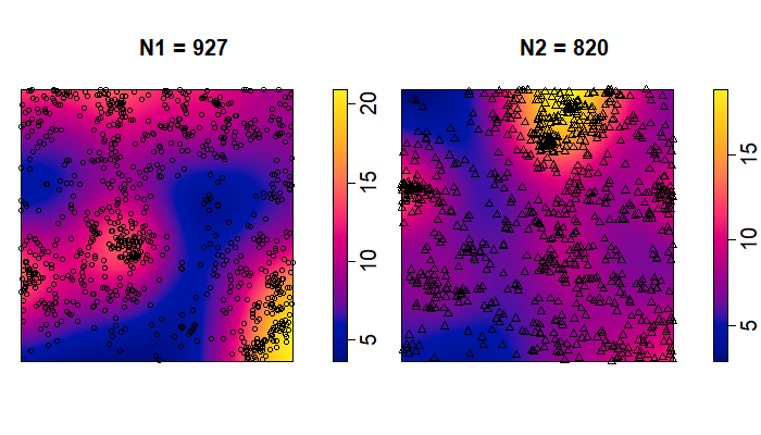
(a) (M1) with $\rho$=0.166.

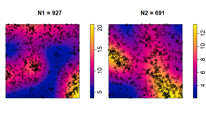
(b) (M1) with $\rho$=-0.166.

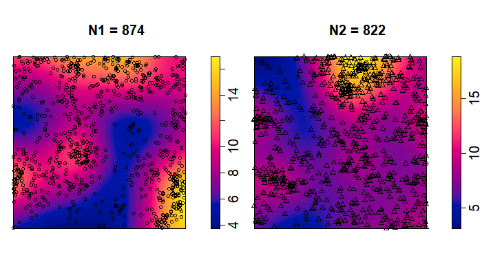
(c) (M2) with $\rho$=0.339.

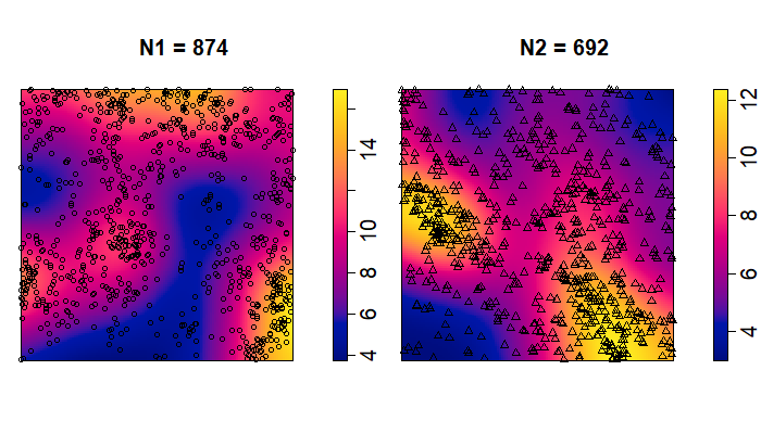
(d) (M2) with $\rho$=-0.339.

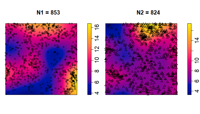
(e) (M3) with $\rho$=0.541.

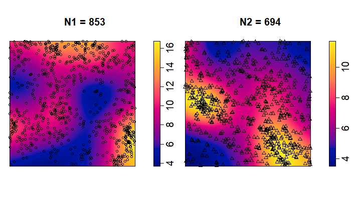
(f) (M3) with $\rho$=-0.541.

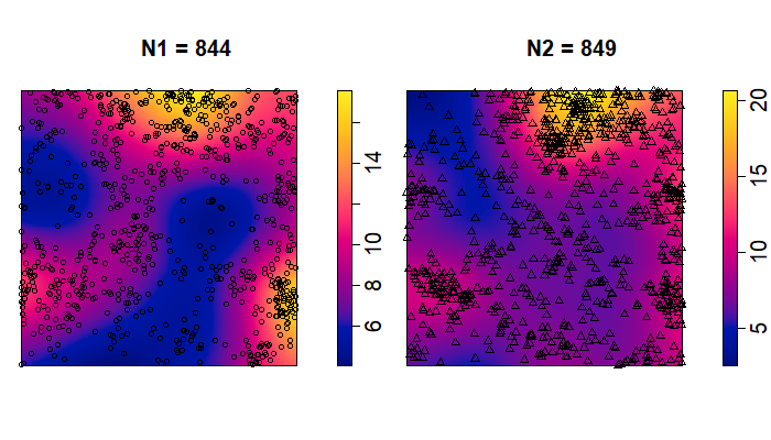
(g) (M4) with $\rho$=0.758.

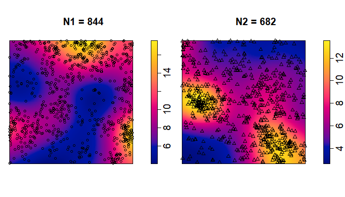
(h) (M4) with $\rho$=-0.758.

Figure E.1: A single realization of the parametric bivariate LGCP models that are considered in Section 6 ($\rho$: correlation coefficient; $\circ$: first process; $\triangle$: second process; $N_{1}$: total number of points of the first process; $N_{2}$: total number of points of the second process). The colored surface indicates the heatmap of the kernel estimate of the intensity function of the point process. Here, we use the sampling window $D=[-5,5]^{2}$ and the common first order intensities $\lambda_{1}^{(1)}=\lambda_{1}^{(2)}=e^{2}\approx 7.38$.

Model	Estimator	Correlation	$R$	Resolution	$\mu=0$	$\mu=1$	$\mu=2$
(M2)	MC	Negative	0.5	–	0.69	1.61	2.68
			2.5	–	1.01	4.60	20.03
			5.0	–	1.05	8.06	24.49
		Positive	0.5	–	0.67	1.50	2.86
			2.5	–	1.20	5.77	21.71
			5.0	–	1.31	10.60	21.92
	MALA	Negative	–	$64\times 64$	2,932.96	2,942.35	2,938.63
			–	$256\times 256$	14,772.07	14,811.62	14,773.65
		Positive	–	$64\times 64$	2,832.09	2,841.97	2,849.68
			–	$256\times 256$	14,494.76	14,447.38	14,402.29
(M3)	MC	Negative	0.5	–	0.67	1.73	2.63
			2.5	–	0.98	4.45	17.42
			5.0	–	1.04	7.58	27.39
		Positive	0.5	–	0.66	1.57	2.80
			2.5	–	1.10	5.29	21.08
			5.0	–	1.15	10.33	24.12
	MALA	Negative	–	$64\times 64$	2,892.79	2,879.04	2,889.51
			–	$256\times 256$	14,891.47	14,891.47	14,801.04
		Positive	–	$64\times 64$	2,821.56	2,778.31	2,794.81
			–	$256\times 256$	14,442.96	14,357.83	14,436.74
(M4)	MC	Negative	0.5	–	0.69	1.86	2.48
			2.5	–	0.98	3.60	14.46
			5.0	–	1.06	6.29	25.02
		Positive	0.5	–	0.72	1.85	3.40
			2.5	–	1.16	5.08	19.83
			5.0	–	1.23	10.34	20.00
	MALA	Negative	–	$64\times 64$	2,938.81	2,934.40	2,940.22
			–	$256\times 256$	14,745.53	14,762.41	14,790.52
		Positive	–	$64\times 64$	2,778.18	2,839.89	2,823.45
			–	$256\times 256$	14,332.03	14,338.86	14,328.37

Table E.1: Similar to Table 2, but for the average computing time of models (M2)–(M4) in Table 1.

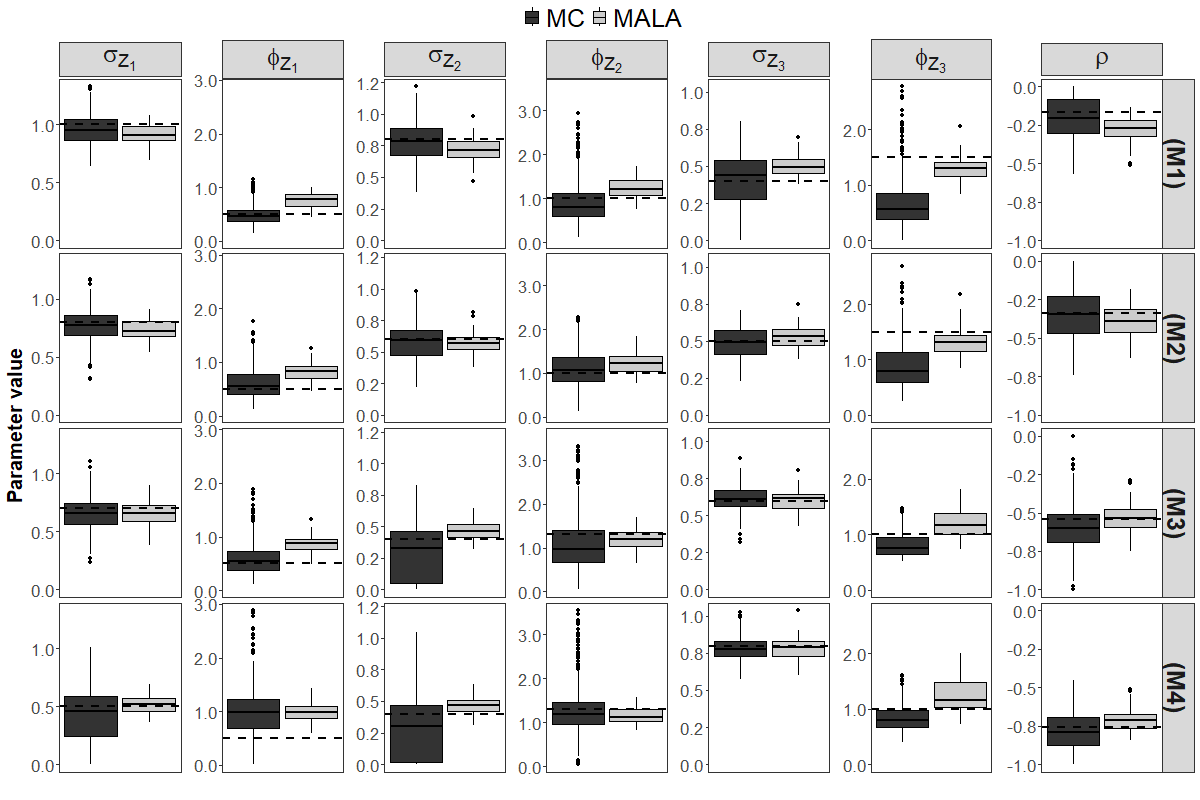
Figure E.2: Box plot of the parameter estimates from MC (colored in dark gray) and MALA using coarse grid (colored in light gray) for negatively correlated models (different rows). For MC, we use the optimal control parameters and exclude any estimates that are outside three standard errors of the true parameter values (marked with horizontal lines).

				Number of Monte Carlo samples of $\bm{V}_{n}(\widehat{\bm{\theta}}_{n})$
Model		Correlation	Experiment	100	300	600	1000
(M1)	Optimal $(c,R)$	Negative	I	(0.1, 2.75)	(0.4, 2.00)	(0.4, 2.75)	(0.5, 2.50)
			II	(0.4, 1.75)	(0.4, 2.50)	(0.1, 2.75)	(0.3, 1.75)
		Positive	I	(0.3, 2.00)	(0.4, 2.50)	(0.4, 2.50)	(0.5, 2.50)
			II	(0.3, 2.00)	(0.3, 2.00)	(0.3, 2.00)	(0.5, 2.50)
	$\log\det\widehat{\Sigma}_{n}(\bm{\theta}_{0})$	Negative	I	-46.04	-48.29	-47.61	-47.81
			II	-47.43	-48.45	-45.21	-45.52
		Positive	I	-43.84	-42.65	-42.64	-40.85
			II	-41.61	-41.47	-41.66	-39.60
	Time (min)	Negative	I	158.68	350.83	638.09	1,025.38
			II	180.92	404.68	642.86	1,048.05
		Positive	I	99.67	177.79	292.81	534.78
			II	98.31	176.52	292.95	544.09
(M2)	Optimal $(c,R)$	Negative	I	(0.4, 1.75)	(0.5, 2.50)	(0.4, 1.75)	(0.4, 1.75)
			II	(0.1, 4.75)	(0.5, 2.25)	(0.4, 1.75)	(0.4, 1.75)
		Positive	I	(0.4, 1.50)	(0.4, 2.75)	(0.4, 2.75)	(0.4, 2.75)
			II	(0.4, 2.75)	(0.4, 2.75)	(0.4, 2.75)	(0.4, 2.75)
	$\log\det\widehat{\Sigma}_{n}(\bm{\theta}_{0})$	Negative	I	-45.27	-49.23	-45.23	-45.31
			II	-44.24	-47.52	-44.94	-45.21
		Positive	I	-44.09	-43.26	-43.32	-43.13
			II	-41.86	-41.54	-41.71	-41.98
	Time (min)	Negative	I	161.09	362.39	631.66	974.58
			II	166.42	365.52	614.48	971.31
		Positive	I	116.75	194.32	311.46	454.20
			II	116.84	192.30	308.58	452.44
(M3)	Optimal $(c,R)$	Negative	I	(0.3, 2.50)	(0.5, 2.00)	(0.3, 2.50)	(0.4, 2.50)
			II	(0.3, 2.75)	(0.5, 4.25)	(0.5, 3.00)	(0.3, 1.75)
		Positive	I	(0.4, 1.75)	(0.4, 1.75)	(0.4, 1.75)	(0.4, 1.75)
			II	(0.4, 1.75)	(0.4, 1.75)	(0.4, 1.75)	(0.4, 1.75)
	$\log\det\widehat{\Sigma}_{n}(\bm{\theta}_{0})$	Negative	I	-47.36	-50.96	-46.99	-46.08
			II	-46.85	-46.81	-47.47	-44.78
		Positive	I	-46.99	-46.04	-45.97	-45.80
			II	-44.82	-44.89	-45.00	-45.10
	Time (min)	Negative	I	138.96	353.21	624.66	1,091.67
			II	175.01	348.92	661.82	890.92
		Positive	I	93.65	177.93	311.75	482.21
			II	94.32	179.72	307.63	472.37
(M4)	Optimal $(c,R)$	Negative	I	(0.2, 1.00)	(0.2, 1.00)	(0.1, 1.00)	(0.1, 1.00)
			II	(0.3, 0.75)	(0.1, 1.00)	(0.1, 1.00)	(0.5, 0.75)
		Positive	I	(0.4, 1.00)	(0.4, 1.00)	(0.4, 1.00)	(0.5, 3.50)
			II	(0.4, 1.00)	(0.4, 1.00)	(0.4, 1.00)	(0.3, 2.75)
	$\log\det\widehat{\Sigma}_{n}(\bm{\theta}_{0})$	Negative	I	-44.83	-44.53	-44.31	-45.74
			II	-44.94	-44.20	-43.76	-46.94
		Positive	I	-49.63	-49.33	-49.39	-48.04
			II	-49.59	-49.43	-49.31	-41.63
	Time (min)	Negative	I	156.09	351.19	616.73	1,109.06
			II	164.70	362.98	654.01	875.27
		Positive	I	118.25	313.00	603.39	1,060.85
			II	137.06	315.30	581.59	915.31

Table E.2: The optimal control parameter $(c,R)$, the log determinant of the estimated asymptotic covariance matrix based on the optimal control parameter, and the total computing time of grid search based on the two realizations (Experiment I and II) for different models and different sizes of Monte Carlo simulations to calculate estimated asymptotic covariance matrix. Here, we set $\mu=2$ for all simulations.

Model	Estimator	Correlation	$\sigma_{Z_{1}}$	$\phi_{Z_{1}}$	$\sigma_{Z_{2}}$	$\phi_{Z_{2}}$	$\sigma_{Z_{3}}$	$\phi_{Z_{3}}$	$\rho$
(M1)	(MC)	Negative	-0.04 (0.13)	-0.01 (0.18)	-0.02 (0.15)	-0.08 (0.46)	-0.01 (0.20)	-0.82 (0.47)	-0.03 (0.14)
		Positive	-0.02 (0.12)	-0.03 (0.17)	-0.02 (0.13)	-0.20 (0.41)	-0.06 (0.24)	0.26 (1.49)	0.03 (0.18)
	(MALA)	Negative	-0.09 (0.10)	0.26 (0.14)	-0.08 (0.10)	0.23 (0.24)	0.10 (0.08)	-0.21 (0.23)	-0.11 (0.09)
		Positive	-0.07 (0.08)	0.28 (0.13)	-0.07 (0.10)	0.27 (0.24)	0.08 (0.07)	-0.27 (0.18)	0.09 (0.07)
(M2)	(MC)	Negative	-0.03 (0.14)	0.12 (0.31)	-0.02 (0.15)	0.10 (0.42)	-0.01 (0.11)	-0.60 (0.42)	-0.01 (0.17)
		Positive	0.006 (0.12)	-0.03 (0.19)	0.003 (0.13)	-0.28 (0.36)	-0.03 (0.19)	0.13 (1.20)	0.03 (0.21)
	(MALA)	Negative	-0.06 (0.10)	0.33 (0.17)	-0.02 (0.09)	0.24 (0.24)	0.02 (0.08)	-0.16 (0.29)	-0.05 (0.10)
		Positive	-0.04 (0.08)	0.34 (0.16)	-0.01 (0.08)	0.26 (0.21)	0.01 (0.07)	-0.18 (0.24)	0.03 (0.08)
(M3)	(MC)	Negative	-0.04 (0.14)	0.09 (0.31)	-0.10 (0.22)	-0.17 (0.61)	0.01 (0.09)	-0.18 (0.23)	-0.05 (0.14)
		Positive	-0.003 (0.11)	0.03 (0.22)	-0.05 (0.18)	-0.46 (0.45)	-0.03 (0.11)	0.05 (0.48)	-0.001 (0.15)
	(MALA)	Negative	-0.05 (0.11)	0.37 (0.17)	0.07 (0.07)	-0.11 (0.21)	-0.004 (0.08)	0.21 (0.26)	0.01 (0.11)
		Positive	-0.03 (0.08)	0.34 (0.16)	0.07 (0.06)	-0.07 (0.19)	-0.01 (0.06)	0.16 (0.22)	-0.03 (0.06)
(M4)	(MC)	Negative	-0.08 (0.25)	0.49 (0.50)	-0.12 (0.25)	-0.02 (0.59)	-0.02 (0.08)	-0.16 (0.23)	-0.03 (0.13)
		Positive	5.8e-5 (0.15)	0.11 (0.23)	-0.09 (0.19)	-0.44 (0.41)	0.03 (0.19)	0.03 (0.18)	0.02 (0.11)
	(MALA)	Negative	0.02 (0.08)	0.49 (0.19)	0.07 (0.07)	-0.14 (0.19)	-0.02 (0.08)	0.22 (0.28)	0.05 (0.07)
		Positive	0.03 (0.08)	0.49 (0.19)	0.07 (0.07)	-0.12 (0.21)	-0.03 (0.07)	0.19 (0.21)	-0.06 (0.06)

Table E.3: Simulation-based bias and standard deviation (in the parenthesis) of the MC and MALA estimator for (M1)–(M4). Here, we use the isotropic edge correction and the optimal $(c,R)$ for MC estimator. The computational grid of MALA is $64\times 64$.

References

• Anderson (2003) Anderson, T. W. (2003), An Introduction to Multivariate Statistical Analysis, John Wiley & Sons, Hokoben, NJ., third edition.
• Ang et al. (2012) Ang, Q. W., Baddeley, A., and Nair, G. (2012), “Geometrically corrected second order analysis of events on a linear network, with applications to ecology and criminology,” Scand. J. Stat., 39, 591–617.
• Baddeley et al. (2007) Baddeley, A., Bárány, I., and Schneider, R. (2007), “Spatial point processes and their applications,” Stochastic Geometry: Lectures Given at the CIME Summer School Held in Martina Franca, Italy, September 13–18, 2004, 1–75.
• Baddeley et al. (2014) Baddeley, A., Jammalamadaka, A., and Nair, G. (2014), “Multitype point process analysis of spines on the dendrite network of a neuron,” J. R. Stat. Soc. Ser. C. Appl. Stat., 63, 673–694.
• Biscio and Svane (2022) Biscio, C. A. N. and Svane, A. M. (2022), “A functional central limit theorem for the empirical Ripley’s K-function,” Electron. J. Stat., 16, 3060–3098.
• Biscio and Waagepetersen (2019) Biscio, C. A. N. and Waagepetersen, R. (2019), “A general central limit theorem and a subsampling variance estimator for $\alpha$-mixing point processes,” Scand. J. Stat., 46, 1168–1190.
• Brillinger (1981) Brillinger, D. R. (1981), Time series: Data Analysis and Theory, vol. 36, SIAM.
• Cox and Lewis (1972) Cox, D. R. and Lewis, P. A. W. (1972), “Multivariate point processes,” in Sixth Berkeley symposium, pp. 401–448.
• Cressie (1993) Cressie, N. (1993), Statistics for Spatial Data, John Wiley & Sons, Hokoben, NJ., revised edition.
• Cui et al. (2018) Cui, Q., Wang, N., and Haenggi, M. (2018), “Vehicle distributions in large and small cities: Spatial models and applications,” IEEE Trans. Veh. Technol., 67, 10176–10189.
• Daley and Vere-Jones (2003) Daley, D. J. and Vere-Jones, D. (2003), An introduction to the theory of point processes: volume I: elementary theory and methods, Springer, New York City, NY., second edition.
• Daley and Vere-Jones (2008) — (2008), An Introduction to the Theory of Point Processes. Volume II: General Theory and Structure, Springer, New York City, NY., second edition.
• Davies and Hazelton (2013) Davies, T. M. and Hazelton, M. L. (2013), “Assessing minimum contrast parameter estimation for spatial and spatiotemporal log-Gaussian Cox processes,” Stat. Neerl., 67, 355–389.
• Diggle (2003) Diggle, P. J. (2003), Statistical Analysis of Spatial Point Patterns, Hodder education publishers, London, UK., second edition.
• Diggle and Gratton (1984) Diggle, P. J. and Gratton, R. J. (1984), “Monte Carlo Methods of Inference for Implicit Statistical Models,” J. R. Stat. Soc. Ser. B. Stat. Methodol., 46, 193–212.
• Doguwa and Upton (1989) Doguwa, S. I. and Upton, G. J. G. (1989), “Edge-corrected estimators for the reduced second moment measure of point processes,” Biometrical Journal, 31, 563–575.
• Doukhan (1994) Doukhan, P. (1994), Mixing: properties and examples, Springer, New York City, NY.
• Fang et al. (1994) Fang, Y., Loparo, K. A., and Feng, X. (1994), “Inequalities for the trace of matrix product,” IEEE Trans. Automat. Control, 39, 2489–2490.
• Fuentes-Santos et al. (2016) Fuentes-Santos, I., González-Manteiga, W., and Mateu, J. (2016), “Consistent smooth bootstrap kernel intensity estimation for inhomogeneous spatial poisson point processes,” Scand. J. Stat., 43, 416–435.
• Gelfand et al. (2004) Gelfand, A. E., Schmidt, A. M., Banerjee, S., and Sirmans, C. F. (2004), “Nonstationary multivariate process modeling through spatially varying coregionalization,” Test, 13, 263–312.
• Girolami and Calderhead (2011) Girolami, M. and Calderhead, B. (2011), “Riemann manifold Langevin and Hamiltonian Monte Carlo methods,” J. R. Stat. Soc. Ser. B. Stat. Methodol., 73, 123–214.
• Guan (2009) Guan, Y. (2009), “A minimum contrast estimation procedure for estimating the second-order parameters of inhomogeneous spatial point processes,” Stat. Interface, 2, 91–99.
• Guan and Sherman (2007) Guan, Y. and Sherman, M. (2007), “On least squares fitting for stationary spatial point processes,” J. R. Stat. Soc. Ser. B. Stat. Methodol., 69, 31–49.
• Guan et al. (2004) Guan, Y., Sherman, M., and Calvin, J. A. (2004), “A nonparametric test for spatial isotropy using subsampling,” J. Amer. Statist. Assoc., 99, 810–821.
• Hanisch and Stoyan (1979) Hanisch, K. H. and Stoyan, D. (1979), “Formulas for the second-order analysis of marked point processes,” Statistics, 10, 555–560.
• Heinrich (1992) Heinrich, L. (1992), “Minimum contrast estimates for parameters of spatial ergodic point processes,” in Transactions of the 11th Prague conference on random processes, information theory and statistical decision functions, Academic Publishing House, pp. 479–492.
• Heinrich and Pawlas (2008) Heinrich, L. and Pawlas, Z. (2008), “Weak and strong convergence of empirical distribution functions from germ-grain processes,” Statistics, 42, 49–65.
• Helmers and Zitikis (1999) Helmers, R. and Zitikis, R. (1999), “On estimation of Poisson intensity functions,” Ann. Inst. Statist. Math., 51, 265–280.
• Jalilian et al. (2015) Jalilian, A., Guan, Y., Mateu, J., and Waagepetersen, R. (2015), “Multivariate product-shot-noise Cox point process models,” Biometrics, 71, 1022–1033.
• Jensen (1993) Jensen, J. L. (1993), “Asymptotic normality of estimates in spatial point processes,” Scand. J. Stat., 97–109.
• Jolivet (1978) Jolivet, E. (1978), “Central limit theorem and convergence of empirical processes for stationary point processes,” in Point processes and queuing problems: Colloquia Mathematica Societatis János Bolyai, vol. 24, pp. 117–161.
• Jun and Cook (2022) Jun, M. and Cook, S. J. (2022), “Flexible multivariate spatio-temporal Hawkes process models of terrorism,” arXiv preprint arXiv:2202.12346.
• Jun et al. (2019) Jun, M., Schumacher, C., and Saravanan, R. (2019), “Global multivariate point pattern models for rain type occurrence,” Spat. Stat., 31, article 100355.
• Kallenberg (1975) Kallenberg, O. (1975), Random measures, Akademie-Verlag, Berlin.
• Kallenberg (2021) — (2021), Foundations of modern probability, Springer, New York City, NY, third edition.
• Karr (2017) Karr, A. (2017), Point processes and their statistical inference, Routledge, Oxfordshire, UK, second edition.
• Kingman (1992) Kingman, J. F. C. (1992), Poisson processes, vol. 3, Oxford University Press, Oxford.
• Lawson (2012) Lawson, A. B. (2012), “Bayesian point event modeling in spatial and environmental epidemiology,” Stat. Methods Med. Res., 21, 509–529.
• Møller (2003) Møller, J. (2003), “Shot noise Cox processes,” Adv. in Appl. Probab., 35, 614–640.
• Møller and Díaz-Avalos (2010) Møller, J. and Díaz-Avalos, C. (2010), “Structured Spatio-Temporal Shot-Noise Cox Point Process Models, with a View to Modelling Forest Fires,” Scand. J. Stat., 37, 2–25.
• Møller et al. (1998) Møller, J., Syversveen, A. R., and Waagepetersen, R. P. (1998), “Log Gaussian Cox processes,” Scand. J. Stat., 25, 451–482.
• Møller and Waagepetersen (2007) Møller, J. and Waagepetersen, R. P. (2007), “Modern spatial point process modelling and inference (with discussion),” Scand. J. Stat., 34, 643–711.
• Nguyen and Zessin (1976) Nguyen, X. X. and Zessin, H. (1976), “Punktprozesse mit Wechselwirkung,” Z. Wahrscheinlichkeitstheorie verw. Gebiete (Probab. Theory Related Fields), 37, 91–126.
• Nguyen and Zessin (1979) — (1979), “Ergodic theorems for spatial processes,” Z. Wahrscheinlichkeitstheorie verw. Gebiete (Probab. Theory Related Fields), 48, 133–158.
• Ogata (1978) Ogata, Y. (1978), “The asymptotic behaviour of maximum likelihood estimators for stationary point processes,” Ann. Inst. Statist. Math., 30, 243–261.
• Pawlas (2009) Pawlas, Z. (2009), “Empirical distributions in marked point processes,” Stochastic Process. Appl., 119, 4194–4209.
• Rajala et al. (2018) Rajala, T., Murrell, D. J., and Olhede, S. C. (2018), “Detecting multivariate interactions in spatial point patterns with Gibbs models and variable selection,” J. R. Stat. Soc. Ser. C. Appl. Stat., 67, 1237–1273.
• Ripley (1976) Ripley, B. D. (1976), “The second-order analysis of stationary point processes,” J. Appl. Probab., 13, 255–266.
• Rue et al. (2009) Rue, H., Martino, S., and Chopin, N. (2009), “Approximate Bayesian inference for latent Gaussian models by using integrated nested Laplace approximations,” J. R. Stat. Soc. Ser. B. Stat. Methodol., 71, 319–392.
• START (2022) START (2022), “Global Terrorism Database 1970 - 2020 [data file],” National Consortium for the Study of Terrorism and Responses to Terrorism, https://www.start.umd.edu/gtd.
• Stoyan et al. (2013) Stoyan, D., Kendall, W. S., Chiu, S. N., and Mecke, J. (2013), Stochastic geometry and its applications, John Wiley & Sons, Hokoben, NJ, 3rd edition.
• Taylor et al. (2015) Taylor, B. M., Davies, T., Rowlingson, B. S., and Diggle, P. J. (2015), “Bayesian Inference and Data Augmentation Schemes for Spatial, Spatiotemporal and Multivariate Log-Gaussian Cox Processes in R,” J. Stat. Softw., 63, 1–48.
• Waagepetersen and Guan (2009) Waagepetersen, R. and Guan, Y. (2009), “Two-step estimation for inhomogeneous spatial point processes,” J. R. Stat. Soc. Ser. B. Stat. Methodol., 71, 685–702.
• Waagepetersen et al. (2016) Waagepetersen, R., Guan, Y., Jalilian, A., and Mateu, J. (2016), “Analysis of multispecies point patterns by using multivariate log-Gaussian Cox processes,” J. R. Stat. Soc. Ser. C. Appl. Stat., 65, 77–96.