On the long-time asymptotic behavior of the Camassa-Holm equation in space-time solitonic regions

Abstract.

In this work, we are devoted to study the Cauchy problem of the Camassa-Holm (CH) equation with weighted Sobolev initial data in space-time solitonic regions

$$m_{t}+2\kappa q_{x}+3qq_{x}=2q_{x}q_{xx}+qq_{xx},~{}~{}m=q-q_{xx}+\kappa,$$

$$q(x,0)=q_{0}(x)\in H^{4,2}(\mathbb{R}),~{}~{}x\in\mathbb{R},~{}~{}t>0,$$

where $\kappa$ is a positive constant. Based on the Lax spectrum problem, a Riemann-Hilbert problem corresponding to the original problem is constructed to give the solution of the CH equation with the initial boundary value condition. Furthermore, by developing the $\bar{\partial}$-generalization of Deift-Zhou nonlinear steepest descent method, different long-time asymptotic expansions of the solution $q(x,t)$ are derived. Four asymptotic regions are divided in this work: For $\xi\in\left(-\infty,-\frac{1}{4}\right)\cup(2,\infty)$, the phase function $\theta(z)$ has no stationary point on the jump contour, and the asymptotic approximations can be characterized with the soliton term confirmed by $N(j_{0})$-soliton on discrete spectrum with residual error up to $O(t^{-1+2\tau})$; For $\xi\in\left(-\frac{1}{4},0\right)$ and $\xi\in\left(0,2\right)$, the phase function $\theta(z)$ has four and two stationary points on the jump contour, and the asymptotic approximations can be characterized with the soliton term confirmed by $N(j_{0})$-soliton on discrete spectrum and the $t^{-\frac{1}{2}}$ order term on continuous spectrum with residual error up to $O(t^{-1})$. Our results also confirm the soliton resolution conjecture for the CH equation with weighted Sobolev initial data in space-time solitonic regions.

1. Introduction

In this work, we study the long-time asymptotic behavior for the initial value problem for the Camassa-Holm (CH) equation:

$$m_{t}+2\kappa q_{x}+3qq_{x}=2q_{x}q_{xx}+qq_{xx},~{}~{}m=q-q_{xx}+\kappa,$$ (1.1)

$$q(x,0)=q_{0}(x)\in H^{4,2}(\mathbb{R}),~{}~{}x\in\mathbb{R},~{}~{}t>0,$$ (1.2)

where $\kappa$ is a positive constant related to the critical shallow water wave speed, and $q=q(x,t)$ is the fluid velocity in the $x$ direction. The CH equation (1.1) is different from the nonlinear Schrödinger type equation which have been extensively researched and has a range of excellent work [1, 25, 26, 41, 42, 43, 44, 49]. At first, the Camassa and Holm in [10] and Camassa, Holm and Hyman in [11] proposed that the equation (1.1) can be applied to describe shallow water waves. It should be pointed out that the CH equation (1.1) has interesting physical meaning. Johson in [30] and Constantin and Lannes in [14] studied the Hydrodynamical relevance of the equation (1.1). Meanwhile, it has rich mathematical structure, for example, it is bi-Hamiltonian and completely integrable [10, 40]. Therefore, various researches on CH equation (1.1) are reported, including local and global well-posedness of its Cauchy problem, blow-up solutions, soliton-type solutions and other works [9, 15, 16]. Moreover, Boutet de Monvel et al. have done many meaningful work on the the equation (1.1), including the Riemann-Hilbert (RH) problem, long-time asymptotic behavior and Painlevé-type asymptotic for the CH equation [4, 5, 7, 8].

The aim of this work is to employ $\bar{\partial}$-steepest descent method to investigate the soliton resolution conjecture of the CH equation (1.1) with the initial value condition

$$q(x,0)=q_{0}(x)\in H^{4,2}(\mathbb{R}),~{}~{}x\in\mathbb{R},~{}~{}t>0,$$

where $H^{k,2}(\mathbb{R})$ are defined in Proposition 2.2.

Inspired by earlier work of Manakov, who have done significant contribution on the research of the long time asymptotic behavior of nonlinear evolution equations by using using the inverse scattering method [36], many researchers continuously follow his step and have done a series of excellent work [12, 27, 31, 32, 39]. Then, Zakharov and Shabat [51] did a series work to develop the RH method by combining inverse scattering method, and the RH method have been widely applied [6]. In 1976, Zakharov and Manakov derived the long time asymptotic solutions of NLS equation with decaying initial value [50]. In 1993, nonlinear steepest descent method was proposed by Defit and Zhou to systematically study the long time asymptotic behavior of nonlinear evolution equations [20]. Over the years, the the nonlinear steepest descent method has been improved and developed . A notable example is that as the initial value is smooth and decays fast enough, the error term is $O(\frac{\ln t}{t})$ shown in [21, 22]. Furthermore, in 2003, Deift and Zhou [19] have shown that the error term is $O(t^{-(\frac{1}{2}+\iota)})$ for any $0<\iota<\frac{1}{4}$ when the initial value belongs to the weighted Sobolev space.

Recently, combining steepest descent with $\bar{\partial}$-problem, McLaughlin and Miller [37, 38] came up with a new idea, i.e., $\bar{\partial}$-steepest descent method, to investigate the asymptotic of orthogonal polynomials. Then, this method was successfully used to investigate defocusing NLS equation with finite mass initial data [23] and with finite density initial data [17]. Notably, compared with the nonlinear steepest descent method, there are some advantages, for example, the delicate estimates involving $L^{p}$ estimates of Cauchy projection operators can be avoided by using $\bar{\partial}$-steepest descent method. Also, the work in [23] shows that the error term is $O(t^{-\frac{3}{4}})$ when the initial value belongs to the weighted Sobolev space. Therefore, a series of great work has been done by applying $\bar{\partial}$-steepest descent method [2, 13, 24, 28, 29, 33, 35, 45, 48].

In this work, our main purpose is to study the Cauchy problem of the CH equation (1.1) with weighted Sobolev initial data $q_{0}(x)\in H^{4,2}(\mathbb{R})$ in space-time solitonic regions. Using a simple transformation

$$x=\tilde{x},\ \ t=\frac{1}{\kappa}\tilde{t},\ \ q(x,t)=\kappa\tilde{q}(\tilde{x},\tilde{t}),$$ (1.3)

the CH equation (1.1) becomes

$$\tilde{m}_{\tilde{t}}+2\tilde{q}_{\tilde{x}}+3\tilde{q}\tilde{q}_{\tilde{x}}=2\tilde{q}_{\tilde{x}}\tilde{q}_{\tilde{x}\tilde{x}}+\tilde{q}\tilde{q}_{\tilde{x}\tilde{x}\tilde{x}},~{}~{}\tilde{m}=\tilde{q}-\tilde{q}_{\tilde{x}\tilde{x}}+1.$$ (1.4)

So without loss of generally, we fix $\kappa=1$.

In our results, with the weighted Sobolev initial data $q_{0}(x)\in H^{4,2}(\mathbb{R})$, we derive the leading order asymptotic approximation for the CH equation (1.1) (see Theorem 10.1 in Section 10):

• For $\xi\in\left(-\infty,-\frac{1}{4}\right)\cup(2,\infty)$,

  $$q(x,t)=q(x,t|D_{j_{0}})+O(t^{-1+2\tau});$$

• For $\xi\in\left(-\frac{1}{4},2\right)$

  $$q(x,t)=q(x,t|D_{j_{0}})+f_{1}t^{-1/2}+O(t^{-1}).$$

Compared with the results in [3], our results are different.

Organization of the rest of the work

In Section 2, based on the Lax pair, the RH problem for $M(z)$ is constructed for the CH equation (1.1) with initial problem..

In Section 3, in order to obtain a a standard RH problem for $M^{(1)}(z)$ with its jump matrix able to be decomposed into two triangle matrices, according to the oscillation term $\exp(2izy-\frac{t}{4z})$ in RH problem 4.1 and applying its sign distribution diagram shown in Fig. 1, we introduce the matrix function $T(z)$.

In Section 4, by using the constructed matrix function $T(z)$, we define a new RH problem for $M^{(1)}(z)$ which admits a regular discrete spectrum and two triangular decompositions of the jump matrix.

In Section 5, we make the continuous extension of the jump matrix off the real axis by introducing a matrix function $R^{(2)}(z)$ and get a mixed $\bar{\partial}$-Riemann-Hilbert(RH) problem for $M^{(2)}(z)$.

In Section 6, we decompose the mixed $\bar{\partial}$-RH problem into two parts that are a model RH problem with $\bar{\partial}R^{(2)}=0$ and a pure $\bar{\partial}$-RH problem with $\bar{\partial}R^{(2)}\neq 0$, i.e., $M^{(2)}_{RHP}$ and $M^{(3)}$.

In Sections 7 and 8, we solve the model RH problem $M^{(2)}_{RHP}$ via an outer model $M^{R}(z)$ for the soliton part and inner model $M^{(loc)}$ near the phase point $\xi_{k}$ which can be solved by matching a model problem on a cross when $\xi\in\left(-\frac{1}{4},2\right)$. While, for $\xi\in\left(-\infty,-\frac{1}{4}\right)\cup(2,\infty)$, $M^{(2)}_{RHP}(z)=E(z)M^{R}(z)$. Also, the error function $E(z)$ with a small-norm RH problem is computed.

In Section 9, the pure $\bar{\partial}$-RH problem for $M^{(3)}$ is studied.

Finally, we obtain the soliton resolution conjecture and long time asymptotic behavior of the CH equation (1.1).

2. The Riemann-Hilbrt problem of CH equation

This section will give the established Riemann-Hilbert problem corresponding the initial value problem for the CH equation (1.1) reported by Boutet de Monvel, Its and Shepelsky [7, 8].

The Lax representation of the CH equation (1.1) has the following form in [10]

$$\begin{split}\psi_{xx}=\frac{1}{4}\psi-\left(z^{2}+\frac{1}{4}\right)m\psi,\\ \psi_{t}=\left(-\frac{2}{1+4z^{2}}-q\right)\psi_{x}+\frac{1}{2}q_{x}\psi,\end{split}$$ (2.1)

where $\psi:=\psi(x,t,z)$ and $z$ is the spectrum paremeter.

Then, the RH problem corresponding to the initial value problem for the CH equation (1.1) is given as follows.

Proposition 2.1.

(see [7, 8]) Let $r(z)$ and $\mathcal{Z}=\{z_{j},\gamma_{j}\}_{j=1}^{N}(Rez_{j}=0,~{}0<Imz_{j}<\frac{1}{2},~{}\gamma_{j}>0)$ be the reflection coefficient and the discrete spectrum with the norming constants $\gamma_{j}$, respectively, corresponding to the initial data $q_{0}(x)$ via the scattering problem for the spectrum problem (2.1).
Let

$$M(y,t;z)=(M_{1}(y,t;z)M_{2}(y,t;z))$$

be the solution of the following RH problem in the complex $z$-plane, $y\in\mathbb{R}$ and $t>0$ being parameters.

Riemann-Hilbert Problem 2.1.

Find an analytic function $M(y,t;z)$ with the following properties:

• $M(y,t;z)$ is meromorphic in $\mathbb{C}\setminus\mathbb{R}$ and continuous to real axis;

• $M(y,t;-z)=M(y,t;z)\sigma_{1}$ where $\sigma_{1}$ is the standard Pauli matrix which can be expressed as

  $$\sigma_{1}=\left(\begin{array}[]{cc}0&1\\ 1&0\\ \end{array}\right),~{}~{}\sigma_{2}=\left(\begin{array}[]{cc}0&-i\\ i&0\\ \end{array}\right),~{}~{}\sigma_{3}=\left(\begin{array}[]{cc}1&0\\ 0&-1\\ \end{array}\right);$$

• $M_{+}(y,t;z)=M_{-}(y,t;z)V(y,t;z)$,   $z\in\mathbb{R}$, where

  $$V(y,t;z)=e^{-iz\left(y-\frac{2t}{1+4z^{2}}\right)\hat{\sigma}_{3}}\left(\begin{array}[]{cc}1-|r(z)|^{2}&-\overline{r(z)}\\ r(z)&1\end{array}\right),$$ (2.4)

  where $e^{\hat{\sigma}_{3}}A$ means $e^{\sigma_{3}}Ae^{-\sigma_{3}}$;

• $M(y,t;z)\to(1~{}~{}1)$ as $z\rightarrow\infty$;

• $M(y,t;z)$ possesses simple poles at each points in $\mathcal{Z}\cup\bar{\mathcal{Z}}$ with:

  $$\begin{split}\mathop{Res}_{z=z_{j}}M(y,t;z)&=\lim_{z\rightarrow z_{j}}M(y,t;z)\left(\begin{array}[]{cc}0&0\\ i\gamma_{j}e^{2it\theta(z_{j})}&0\end{array}\right),\\ \mathop{Res}_{z=\bar{z}_{j}}M(y,t;z)&=\lim_{z\rightarrow\bar{z}_{j}}M(y,t;z)\left(\begin{array}[]{cc}0&-i\gamma_{j}e^{-2it\theta(\bar{z}_{j})}\\ 0&0\end{array}\right).\end{split}$$ (2.5)

  where $\theta(y,t,z)=z\left(\frac{y}{t}-\frac{2}{1+4z^{2}}\right)$.

Then, according to the RH problem 2.1, the solution $q(x,t)$ of the initial value problem (1.1) can be expressed in a parametric form

$$x(y,t) =y+\ln\frac{M_{1}(y,t;\frac{i}{2})}{M_{2}(y,t;\frac{i}{2})},$$ (2.6)

$$q(y,t) =\frac{1}{2i}\lim_{z\to\frac{i}{2}}\left(\frac{M_{1}(y,t;z)M_{2}(y,t;z)}{M_{1}(y,t;\frac{i}{2})M_{2}(y,t;\frac{i}{2})}-1\right)\frac{1}{z-\frac{i}{2}}.$$ (2.7)

Alternatively,

$$q(y,t)=\frac{\partial}{\partial t}\ln\frac{M_{1}(y,t;\frac{i}{2})}{M_{2}(y,t;\frac{i}{2})}.$$

Remark 2.2.

On the basis of the Zhou’s vanishing lemma [53], the existence of the solutions of RHP 2.1 for $x\in\mathbb{R},t>0$ is guaranteed. According to the results of Liouville’s theorem, we know that if the solution of RH problem 2.1 exists, it is unique.

Proposition 2.2.

If the initial data $q_{0}(x)\in H^{4,2}(\mathbb{R})$, then $r(z)\in H^{1,1}(\mathbb{R})$. The space $H^{4,2}(\mathbb{R})$ is defined as

$$H^{k,2}(\mathbb{R})=\left\{f(x)\in L^{p}(\mathbb{R}):x^{2}\partial^{j}f(x)\in L^{p}(\mathbb{R}),j=1,2,\ldots,k\right\}.$$

3. Conjugation

According to the jump matrix (2.4), we know that the oscillation term is

$$e^{2iz\left(y-\frac{2t}{1+4z^{2}}\right)}=e^{2it\theta(z)},~{}~{}\theta(z)=z\left(\frac{y}{t}-\frac{2}{1+4z^{2}}\right).$$ (3.1)

It is obvious to observe that the growth and decay of the exponential function $e^{2it\theta(z)}$ have great effect on the long-time asymptotic of RH problem 2.1. Therefore, we introduce a transformation $M(z)\rightarrow M^{(1)}(z)$ to make the $M^{(1)}(z)$ is well behaved as $|t|\rightarrow\infty$ along any characteristic line.

Let $\xi=\frac{y}{t}$, the stationary phase points, i.e., $\theta^{\prime}(z)=0$, are given by $\pm z_{0}$ and $\pm z_{1}$ where

$$z_{0}=\frac{1}{2}\sqrt{-\frac{\xi+1-\sqrt{1+4\xi}}{\xi}},$$

$$z_{1}=\frac{1}{2}\sqrt{-\frac{\xi+1+\sqrt{1+4\xi}}{\xi}}.$$

In order to study the asymptotic behavior of $e^{2it\theta(z)}$ as $t\to\infty$, we evaluate the real part of $2it\theta(z)$:

$$Rez(i\theta)=-Imz\xi-\frac{16Rez^{2}Imz-2Imz(1+4Rez^{2}-4Imz^{2})}{(1+4Rez^{2}-4Imz^{2})^{2}+(8RezImz)^{2}}.$$ (3.2)

The properties of $Re(i\theta)$ are shown in Fig. 1

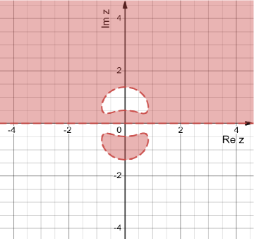
($a$)                     ($b$)

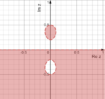
($c$)                     ($d$)

Figure 1. (Color online) The classification of sign $Re(2i\theta(z))$. In the pink regions, $Re(2i\theta(z))>0$, which implies that $e^{-2it\theta(z)}\to 0$ as $t\to\infty$. While in the white regions, $Re(2i\theta(z))<0$, which implies $e^{2it\theta(z)}\to 0$ as $t\to\infty$. The red curves $Re(2i\theta(z))=0$ are critical lines between decay and growth regions.

Therefore, there are four cases are distinguished as

1. For $\xi>2$, $z_{0},z_{1}\notin\mathbb{R}$ corresponding to Fig. 1($d$);

2. For $0<\xi<2$, $z_{0}\in\mathbb{R},z_{1}\notin\mathbb{R}$ corresponding to Fig. 1($c$);

3. For $-\frac{1}{4}<\xi<0$, $z_{0},z_{1}\in\mathbb{R}$ corresponding to Fig. 1($b$);

4. For $\xi<-\frac{1}{4}$, $z_{0},z_{1}\notin\mathbb{R}$ corresponding to Fig. 1($a$).

Next, for convenience, we introduce some notations. Let $\xi_{1}=z_{1}$, $\xi_{2}=z_{0}$, $\xi_{3}=-z_{0}$, $\xi_{4}=-z_{1}$. Define

$$I(\xi)=\left\{\begin{aligned} &\mathbb{R},&\xi\in(-\infty,-\frac{1}{4}),\\ &(-\infty,\xi_{4})\cup(\xi_{3},\xi_{2})\cup(\xi_{4},\infty),&\xi\in(-\frac{1}{4},0),\\ &(\xi_{3},\xi_{2}),&\xi\in(0,2),\\ &\emptyset,&\xi\in(2,\infty).\end{aligned}\right.$$

Denote

$$n(\xi)=\left\{\begin{aligned} &0,&\xi\in(-\infty,-\frac{1}{4})\cup(2,\infty),\\ &2,&\xi\in(-\frac{1}{4},0),\\ &4,&\xi\in(0,2).\end{aligned}\right.$$

Define

$$\rho=\frac{1}{3}\min_{z_{j}\in\mathcal{Z},j\neq k}\{z_{j}-z_{k}\},$$ (3.3)

$$\mathcal{N}=\{1,2,\ldots,N\},$$ (3.4)

$$j_{0}=j_{0}(\xi)=\left\{\begin{aligned} &j,~{}~{}if~{}|\frac{1}{2}-Imz_{j}|<\rho,~{}~{}or~{}~{}|\kappa_{0}-Imz_{j}|<\rho,~{}j\in\{1,2,\ldots,N\},~{}~{}for~{}~{}\xi\in(2,\infty),\\ &j,~{}~{}if~{}|\frac{1}{2}-Imz_{j}|<\rho,~{}j\in\{1,2,\ldots,N\},~{}~{}for~{}~{}\xi\in(-\infty,2),\\ &-1,~{}~{}otherwise.\end{aligned}\right.$$ (3.5)

It is noted that the discrete spectrum points $z_{j}(j=1,2,\ldots,N)$ are distribute in $i(0,\frac{1}{2})$, which means the discrete spectrum points $z_{j}(j=1,2,\ldots,N)$ are distribute in the positive region $Re(2i\theta(z))>0$ for $\xi<2$. For $\xi>2$, a part of discrete spectrum points is distribute in the positive region $Re(2i\theta(z))>0$ and another part is distribute in the negative region $Re(2i\theta(z))<0$.

Therefore, we further define functions

$$\delta(z): =\delta(z,\xi)=\exp\left(i\int_{I(\xi)}\frac{\nu(s)}{s-z}\,ds\right),~{}~{}\nu(s)=-\frac{1}{2\pi}\log(1+|r(s)|^{2}),$$ (3.6)

$$T(z): =T(z,\xi)=\left\{\begin{aligned} &\prod_{k=1}^{N}\frac{(z-\bar{z}_{k})}{(z-z_{k})}\delta(z),&\xi<2,\\ &\prod_{\kappa_{0}<Imz_{k}<\frac{1}{2}}\frac{(z-\bar{z}_{k})}{(z-z_{k})}\delta(z),&\xi>2.\end{aligned}\right.$$ (3.7)

where $\kappa_{0}=\frac{1}{2}\sqrt{1-\frac{2}{\xi}}$.

Then, we show the properties of the function $T(z)$.

Proposition 3.1.

The functions $T(z)$ satisfies that
($a$) $T(z)$ is meromorphic in $C\setminus\mathbb{R}$;
($b$) For $z\in C\setminus\mathbb{R}$, $\bar{T}(\bar{z})=T(-z)$;
($c$) For $z\in C\setminus I(\xi)$, $T^{-1}(z)=T(-z)$;
($d$) For $z\in I(\xi)$, the boundary values $T_{\pm}$ satisfies that

$$\frac{T_{+}(z)}{T_{-}(z)}=1-|r(z)|^{2},z\in I(\xi);$$ (3.8)

($e$) $T(\infty):=\lim\limits_{z\rightarrow\infty}T(z)=1$;
($f$) As $z\rightarrow\frac{i}{2}$, $T(z)$ can be expressed as

$$T(z)=T(\frac{i}{2})(\mathbb{I}+(z-\frac{i}{2})T_{1})+O((z-\frac{i}{2})^{2}),$$ (3.9)

where $T_{1}=2i\sum\frac{2iIm~{}z_{j}}{\frac{1}{4}-Imz^{2}_{j}}-\frac{1}{2\pi i}\int_{I(\xi)}\frac{\log(1-|r(s)|^{2}}{(s-z)^{2}}\,ds$;
($g$) As $z\rightarrow\xi_{j}(j=1,2,3,4)$ along any ray $\xi_{j}+e^{i\phi}R_{+}$ with $|\phi|\leq c<\pi$,

$$\left|T(z,\xi)-T_{j}(\xi)(z-\xi_{j})^{i\nu(\xi_{j})}\right|\lesssim||r||_{H^{1,1}(\mathbb{R})}|z-\xi_{j}|^{\frac{1}{2}},$$ (3.10)

where

$$T_{j}(\xi_{j})=\prod\frac{\xi_{j}+iImz_{j}}{\xi_{j}-iImz_{j}}e^{i\beta(\xi_{j},\xi_{j})},$$ (3.11)

with

$$\beta(z,\xi_{j})=\nu(\xi_{j})\log(z-\xi_{j}+1)+\int_{I(\xi)}\frac{\nu(s)}{s-z}\,ds.$$ (3.12)

Proof.

The above properties of $T(z)$ can be proved by a direct calculation, for details, see [2, 34]. ∎

4. Deformation of Riemann-Hilbert problem

In order to trade the poles for jumps on small contours encircling the pole $z_{j}(j\neq j_{0})$ (see Fig. 2) and deform the Riemann-Hilbert problem 2.1, through employing the function $T(z)$, we introduce the following transformation: for $\xi\in(-\infty,2)$ and $j\neq j_{0}$,

$$M^{(1)}(y,t,z)=\left\{\begin{aligned} &M(y,t,z)\left(\begin{array}[]{cc}1&-\frac{z-iImz_{j}}{i\gamma_{j}e^{2it\theta(iImz_{j})}}\\ 0&1\\ \end{array}\right)T(z)^{-\sigma_{3}},~{}~{}&|z-iImz_{j}|<\rho,\\ &M(y,t,z)\left(\begin{array}[]{cc}1&0\\ \frac{z+iImz_{j}}{i\gamma_{j}e^{-2it\theta(-iImz_{j})}}&1\\ \end{array}\right)T(z)^{-\sigma_{3}},~{}~{}&|z+iImz_{j}|<\rho,\\ &M(y,t,z)T(z)^{-\sigma_{3}},\qquad&elsewhere,\end{aligned}\right.$$ (4.1)

for $\xi\in(2,\infty)$ and $j\neq j_{0}$,

$$M^{(1)}(y,t,z)=\left\{\begin{aligned} &M(y,t,z)\left(\begin{array}[]{cc}1&-\frac{z-iImz_{j}}{i\gamma_{j}e^{2it\theta(iImz_{j})}}\\ 0&1\\ \end{array}\right)T(z)^{-\sigma_{3}},~{}~{}&|z-iImz_{j}|<\rho,~{}~{}\kappa_{0}<Imz_{j}<\frac{1}{2},\\ &M(y,t,z)\left(\begin{array}[]{cc}1&0\\ -\frac{-i\gamma_{j}e^{2it\theta(iImz_{j})}}{z-iImz_{j}}&1\\ \end{array}\right)T(z)^{-\sigma_{3}},~{}~{}&|z-iImz_{j}|<\rho,~{}~{}0<Imz_{j}<\kappa_{0},\\ &M(y,t,z)\left(\begin{array}[]{cc}1&0\\ \frac{z+iImz_{j}}{i\gamma_{j}e^{-2it\theta(-iImz_{j})}}&1\\ \end{array}\right)T(z)^{-\sigma_{3}},~{}~{}&|z+iImz_{j}|<\rho,~{}~{}\kappa_{0}<Imz_{j}<\frac{1}{2},\\ &M(y,t,z)\left(\begin{array}[]{cc}1&\frac{i\gamma_{j}e^{-2it\theta(-iImz_{j})}}{z+iImz_{j}}\\ 0&1\\ \end{array}\right)T(z)^{-\sigma_{3}},~{}~{}&|z+iImz_{j}|<\rho,~{}~{}0<Imz_{j}<\kappa_{0},\\ &M(y,t,z)T(z)^{-\sigma_{3}},\qquad&elsewhere.\end{aligned}\right.$$ (4.2)

Figure 2. (Color online) The contour of the regular RH problem.

Then, we obtain a matrix RH problem for $M^{(1)}(z)$.

Riemann-Hilbert Problem 4.1.

Find a matrix function $M^{(1)}(y,t,z)$ with the following properties:

• $M^{(1)}(y,t,z)$ is meromorphic in $\mathbb{C}\setminus\Sigma^{(\xi,1)}$, where

  $$\Sigma^{(\xi,1)}=\mathbb{R}\cup\left(\bigcup_{j\in\{1,2,\ldots,N\},j\neq j_{0}}\{z\in\mathbb{C}:|z-iImz_{j}|=\rho~{}or~{}|z+iImz_{j}|=\rho\}\right);$$

• $M^{(1)}(y,t;-z)=M^{(1)}(y,t;z)\sigma_{1}$;

• $M^{(1)}(y,t;z)\to(1~{}~{}1)$ as $z\rightarrow\infty$;

• For $z\in\Sigma^{(\xi,1)}$, the boundary values $M^{(1)}_{\pm}(y,t,z)$ satisfy the jump relationship $M^{(1)}_{+}(y,t,z)=M^{(1)}_{-}(y,t,z)V^{(1)}(z)$, where for $\xi\in(-\infty,2)$,

  $$V^{(1)}(z)=\left\{\begin{aligned} &\left(\begin{array}[]{cc}1&-\overline{r(z)}T(z)^{2}e^{-2it\theta(z)}\\ 0&1\\ \end{array}\right)\left(\begin{array}[]{cc}1&0\\ r(z)T(z)^{-2}e^{2it\theta(z)}&1\\ \end{array}\right),~{}~{}z\in\mathbb{R}\setminus I(\xi)\\ &\left(\begin{array}[]{cc}1&0\\ \frac{r(z)T_{-}(z)^{-2}}{1-|r(z)|^{2}}e^{2it\theta(z)}&1\\ \end{array}\right)\left(\begin{array}[]{cc}1&\frac{-\overline{r(z)}T_{+}(z)^{2}}{1-|r(z)|^{2}}e^{-2it\theta(z)}\\ 0&1\\ \end{array}\right),~{}~{}z\in I(\xi),\\ &\left(\begin{array}[]{cc}1&-\frac{z-iImz_{j}}{i\gamma_{j}e^{2it\theta(iImz_{j})}}T(z)^{2}\\ 0&1\\ \end{array}\right),~{}~{}|z-iImz_{j}|=\rho,~{}j\neq j_{0},\\ &\left(\begin{array}[]{cc}1&0\\ -\frac{z+iImz_{j}}{i\gamma_{j}e^{-2it\theta(-iImz_{j})}}T(z)^{-2}&1\\ \end{array}\right),~{}~{}|z+iImz_{j}|=\rho,~{}j\neq j_{0},\end{aligned}\right.$$ (4.3)

  for $\xi\in(2,\infty)$,

  $$V^{(1)}(z)=\left\{\begin{aligned} &\left(\begin{array}[]{cc}1&-\overline{r(z)}T(z)^{2}e^{-2it\theta(z)}\\ 0&1\\ \end{array}\right)\left(\begin{array}[]{cc}1&0\\ r(z)T(z)^{-2}e^{2it\theta(z)}&1\\ \end{array}\right),~{}~{}z\in\mathbb{R}\\ &\left(\begin{array}[]{cc}1&-\frac{z-iImz_{j}}{i\gamma_{j}e^{2it\theta(iImz_{j})}}T(z)^{2}\\ 0&1\\ \end{array}\right),~{}~{}|z-iImz_{j}|=\rho,~{}~{}\kappa_{0}<Imz_{j}<\frac{1}{2},~{}j\neq j_{0},\\ &\left(\begin{array}[]{cc}1&0\\ -\frac{i\gamma_{j}e^{2it\theta(iImz_{j})}}{z-iImz_{j}}T(z)^{-2}&1\\ \end{array}\right),~{}~{}|z-iImz_{j}|=\rho,~{}~{}0<Imz_{j}<\kappa_{0},~{}j\neq j_{0},\\ &\left(\begin{array}[]{cc}1&0\\ -\frac{z+iImz_{j}}{i\gamma_{j}e^{-2it\theta(-iImz_{j})}}T(z)^{-2}&1\\ \end{array}\right),~{}~{}|z+iImz_{j}|=\rho,~{}~{}\kappa_{0}<Imz_{j}<\frac{1}{2},~{}j\neq j_{0},\\ &\left(\begin{array}[]{cc}1&-\frac{i\gamma_{j}e^{-2it\theta(-iImz_{j})}}{z+iImz_{j}}T(z)^{2}\\ 0&1\\ \end{array}\right),~{}~{}|z+iImz_{j}|=\rho,~{}~{}0<Imz_{j}<\kappa_{0},~{}j\neq j_{0};\end{aligned}\right.$$ (4.4)

• $M^{(1)}(y,t,z)$ has simple poles at each $z_{j}\in\mathcal{Z}(j=j_{0})$ at which for $\xi\in(-\infty,2)$,

  $$\begin{split}\mathop{Res}\limits_{z=z_{j_{0}}}M^{(1)}(y,t,z)=\lim_{z\rightarrow z_{j_{0}}}M^{(1)}(y,t,z)\left(\begin{array}[]{cc}0&i\gamma_{j_{0}}e^{-2it\theta(z_{j_{0}})}\frac{1}{T}^{\prime}(z_{j_{0}})^{-2}\\ 0&0\\ \end{array}\right),\\ \mathop{Res}\limits_{z=\bar{z}_{j_{0}}}M^{(1)}(y,t,z)=\lim_{z\rightarrow\bar{z}_{j_{0}}}M^{(1)}(y,t,z)\left(\begin{array}[]{cc}0&0\\ i\gamma^{-1}_{j_{0}}e^{2it\theta(\bar{z}_{j_{0}})}T^{\prime}(\bar{z}_{j_{0}})^{-2}&0\\ \end{array}\right);\end{split}$$ (4.5)

  For $\xi\in(2,\infty)$, if $\kappa_{0}<Imz_{j_{0}}<\frac{1}{2}$, the residue conditions are the same with (4.5); if $0<Imz_{j_{0}}<\kappa_{0}$, the residue conditions are that

  $$\begin{split}\mathop{Res}\limits_{z=z_{j_{0}}}M^{(1)}(y,t,z)=\lim_{z\rightarrow z_{j_{0}}}M^{(1)}(y,t,z)\left(\begin{array}[]{cc}0&0\\ i\gamma_{j_{0}}e^{2it\theta(z_{j_{0}})}T^{-2}(z_{j_{0}})&0\\ \end{array}\right),\\ \mathop{Res}\limits_{z=\bar{z}_{j_{0}}}M^{(1)}(y,t,z)=\lim_{z\rightarrow\bar{z}_{j_{0}}}M^{(1)}(y,t,z)\left(\begin{array}[]{cc}0&i\gamma_{j_{0}}e^{-2it\theta(\bar{z}_{j_{0}})}T^{2}(\bar{z}_{j_{0}})\\ 0&0\\ \end{array}\right).\end{split}$$ (4.6)

Proof.

According to the definition of $M^{(1)}(y,t,z)$, applying Proposition 3.1, the analyticity, jump matrix and asymptotic behavior of $M^{(1)}$ are derived directly. Moreover, the residue condition of $M^{(1)}(y,t,z)$ can be derived by a similar calculation. ∎

Then, according to the RH problem 4.1, the solution $q(x,t)$ of the initial value problem (1.1) can be expressed in a parametric form

$$\begin{split}x(y,t)&=y+\ln\frac{M^{(1)}_{1}(y,t;\frac{i}{2})}{M^{(1)}_{2}(y,t;\frac{i}{2})},\\ q(y,t)&=\frac{1}{2i}\lim_{z\to\frac{1}{2}}\left(\frac{M^{(1)}_{1}(y,t;z)M^{(1)}_{2}(y,t;z)}{M^{(1)}_{1}(y,t;\frac{i}{2})M^{(1)}_{2}(y,t;\frac{i}{2})}-1\right)\frac{1}{z-\frac{i}{2}}.\end{split}$$ (4.7)

5. The $\bar{\partial}$ extensions of jump factorization

The goal of this section is to removing the jump from the real axis $\mathbb{R}$ in new lines along which the $e^{2it\theta(z)}$ is decay/growth for $z\notin\mathbb{R}$. To approach this goal, we first introduce some regions and contours with respect to $\xi$.

Fix a angle $\theta_{0}$ (small enough) such that the set $\{z\in\mathbb{C}:~{}\cos\theta_{0}<\big{|}\frac{Rez}{z}\big{|}\}$ does not intersect the boundary $Re(i\theta(z))=0$. Define

$$\phi=\min\{\theta_{0},~{}\frac{\pi}{4}\}.$$

• For $\xi\in(-\infty,-\frac{1}{4})\cup(2,\infty)$, following the idea in [7, 47], let $\varepsilon_{0}$ be an sufficiently small positive constant such that the circles $\{|z-z_{j}|=\rho,|z-\bar{z}_{j}|=\rho\}$ around $z_{j}$ and $\bar{z}_{j}$ lie outside the region $\{z||Imz|<\varepsilon_{0}\}$. Then, we define $\Omega(\xi)=\bigcup_{k=1}^{4}\Omega_{k}$ where $\Omega_{k}=\Omega_{k0}\cup\Omega_{k1}$ (see Fig. 3) with

  $$\Omega_{10}=\{z:Rez>0,0<Imz<\varepsilon_{0}\},~{}~{}\Omega_{11}=\{z:\arg(z-i\varepsilon_{0})\in(0,\phi)\},$$

  $$\Omega_{20}=\{z:Rez<0,0<Imz<\varepsilon_{0}\},~{}~{}\Omega_{21}=\{z:\arg(z-i\varepsilon_{0})\in(\pi-\phi,\pi)\},$$

  $$\Omega_{30}=\{z:Rez>0,-\varepsilon_{0}<Imz<0\},~{}~{}\Omega_{31}=\{z:\arg(z+i\varepsilon_{0})\in(-\pi,-\pi+\phi)\},$$

  $$\Omega_{40}=\{z:Rez<0,-\varepsilon_{0}<Imz<0\},~{}~{}\Omega_{41}=\{z:\arg(z+i\varepsilon_{0})\in(-\phi,0)\}.$$

  Denote

  $$\begin{split}\Sigma_{1}=i\varepsilon_{0}+e^{i\phi}\mathbb{R}_{+},~{}~{}~{}~{}~{}~{}\Sigma_{2}=i\varepsilon_{0}+e^{i(\pi-\phi)}\mathbb{R}_{+},\\ \Sigma_{3}=-i\varepsilon_{0}+e^{-i(\pi-\phi)}\mathbb{R}_{+},~{}~{}\Sigma_{4}=-i\varepsilon_{0}+e^{-i\phi}\mathbb{R}_{+}.\end{split}$$ (5.1)

  Define

  $$\tilde{\Sigma}(\xi)=\Sigma_{1}\cup\Sigma_{2}\cup\Sigma_{3}\cup\Sigma_{4},$$

  $$\Sigma^{(\xi,2)}=\tilde{\Sigma}(\xi)\cup\left(\bigcup_{j\in\mathcal{N},j\neq j_{0}}\{|z-z_{j}|=\rho,|z-\bar{z}_{j}|=\rho\}\right),$$

  where $\mathcal{N}=\{1,2,\ldots,N\}$.

• For $\xi\in(-\frac{1}{4},0)$ (see Fig.4), we define

  $$\Sigma_{jk}(\xi)=\left\{\begin{aligned} &\xi_{j}+e^{i(\pi+(-1)^{k}\phi)},~{}~{}k=1,2,\\ &\xi_{j}+e^{i(2\pi+(-1)^{k}\phi)},~{}~{}k=3,4,\end{aligned}\right.$$

  where $j=1,3,$ and for $j=2,3,$

  $$\Sigma_{jk}(\xi)=\left\{\begin{aligned} &\xi_{j}+e^{i(-1)^{k-1}\phi},~{}~{}k=1,2,\\ &\xi_{j}+e^{i(\pi+(-1)^{k-1}\phi)},~{}~{}k=3,4,\end{aligned}\right.$$

  For $j=2,3,4$, we define

  $$\Sigma^{\prime}_{j,\pm}=\frac{\xi_{j}+\xi{j-1}}{2}\pm e^{i\frac{\pi}{2}}\ell_{j},$$

  where $\ell_{j}\in(0,\frac{|\xi_{j}-\xi_{j-1}|}{2}\tan\phi).$ Then, we can further define

  $$\Omega(\xi) =\bigcup_{j,k=1,2,3,4}\Omega_{jk},~{}~{}\Omega_{\pm}=\mathbb{C}\setminus\Omega(\xi),$$

  $$\tilde{\Sigma}(\xi) =\left(\bigcup_{j,k=1,2,3,4}\Sigma_{jk}\right)\cup\left(\bigcup_{j=2,3,4}\Sigma^{\prime}_{j,\pm}\right).$$

  $$\Sigma^{(\xi,2)} =\tilde{\Sigma}(\xi)\cup\left(\bigcup_{j\in\mathcal{N},j\neq j_{0}}\{|z-z_{j}|=\rho,|z-\bar{z}_{j}|=\rho\}\right).$$

• For $\xi\in(0,2)$ (see Fig.4), we define

  $$\Sigma_{1k}(\xi) =\left\{\begin{aligned} &\xi_{2}+e^{i(-1)^{k-1}\phi},~{}~{}k=1,2,\\ &\xi_{2}+e^{i(\pi+(-1)^{k-1}\phi)},~{}~{}k=3,4,\end{aligned}\right.$$

  $$\Sigma_{2k}(\xi) =\left\{\begin{aligned} &\xi_{3}+e^{i(\pi+(-1)^{k}\phi},~{}~{}k=1,2,\\ &\xi_{3}+e^{i(-1)^{k-1}\phi},~{}~{}k=3,4,\end{aligned}\right.$$

  $$\Sigma^{\prime}_{3,\pm}(\xi) =\pm e^{i\frac{\pi}{2}}\ell_{3},$$

  where $\ell_{3}\in(0,\frac{|\xi_{3}-\xi_{2}|}{2}\tan\phi).$ Then, we can further define

  $$\Omega(\xi) =\bigcup_{j=1,2,k=1,2}\Omega_{jk},~{}~{}\Omega_{\pm}=\mathbb{C}\setminus\Omega(\xi),$$

  $$\tilde{\Sigma}(\xi) =\left(\bigcup_{j=1,2,k=1,2}\Sigma_{jk}\right)\cup\Sigma^{\prime}_{3,\pm}.$$

  $$\Sigma^{(\xi,2)} =\tilde{\Sigma}(\xi)\cup\left(\bigcup_{j\in\mathcal{N},j\neq j_{0}}\{|z-z_{j}|=\rho,|z-\bar{z}_{j}|=\rho\}\right).$$

Figure 3. The new regions $\Omega(\xi)(\xi\in(-\infty,-\frac{1}{4})\cup(2,\infty))$ and the contours $\Sigma_{k}$.

Figure 4. Figure (a) and (b) are corresponding to the $\xi\in(-\frac{1}{4},0)$ and $\xi\in(0,2)$ respectively. The regions $\Omega_{jk}$ are of the boundaries $\Sigma_{jk}$.

In what follows, we introduce extensions of the off-diagonal entries of jump matrices of (4.3) and (4.4). To approach this purpose, we construct matrix function $R^{(2)}(z,\xi)$ and control the norm of $\bar{\partial}R^{(2)}(z,\xi)$ to ensure that $\bar{\partial}$-contribution has little impact on the long-time asymptotic solution of $q(x,t)$. It is observed that $\theta(z)$ has different properties in different regions, so we have to construct different $R^{(2)}(z,\xi)$ in different regions. Next, we construct $R^{(2)}(z,\xi)$ as
$\bullet$ For $\xi\in(-\infty,-\frac{1}{4})$,

$$R^{(2)}(z,\xi)=\left\{\begin{aligned} &\left(\begin{array}[]{cc}1&R_{j}(\xi)e^{-2it\theta(z)}\\ 0&1\\ \end{array}\right),~{}~{}&z\in\Omega_{j},~{}~{}j=1,2,\\ &\left(\begin{array}[]{cc}1&0\\ R_{j}(\xi)e^{-2it\theta}&1\\ \end{array}\right),~{}~{}&z\in\Omega_{j},~{}~{}j=3,4,\\ &\left(\begin{array}[]{cc}1&0\\ 0&1\\ \end{array}\right),~{}~{}&z\in~{}~{}elsewhere.\end{aligned}\right.$$ (5.2)

$\bullet$ For $\xi\in(2,\infty)$,

$$R^{(2)}(z,\xi)=\left\{\begin{aligned} &\left(\begin{array}[]{cc}1&0\\ R_{j}(\xi)e^{2it\theta(z)}&1\\ \end{array}\right),~{}~{}&z\in\Omega_{j},~{}~{}j=1,2,\\ &\left(\begin{array}[]{cc}1&R_{j}(\xi)e^{-2it\theta}\\ 0&1\\ \end{array}\right),~{}~{}&z\in\Omega_{j},~{}~{}j=3,4,\\ &\left(\begin{array}[]{cc}1&0\\ 0&1\\ \end{array}\right),~{}~{}&z\in~{}~{}elsewhere.\end{aligned}\right.$$ (5.3)

In the above formulae, $R_{j}(\xi)(j=1,2,3,4)$ is defined in the following proposition.

Proposition 5.1.

There exist functions $R_{j}:\bar{\Omega}_{j}\rightarrow C,j=1,2,3,4$ with boundary values such that,
$\bullet$ for $\xi\in(-\infty,-\frac{1}{4})$,

$$R_{j}(z,\xi)(j=1,2)=\left\{\begin{aligned} &-\frac{\overline{r(z)}}{1-|r(z)|^{2}}T_{+}^{2}(z)\triangleq p_{j}(z,\xi)T_{+}^{2}(z),&z\in\mathbb{R},\\ &-\frac{\overline{r(0)}}{1-|r(0)|^{2}}T_{0}^{2}(0)z^{2i\nu(0)},&z\in\Sigma_{1}\cup\Sigma_{2},\end{aligned}\right.$$

$$R_{j}(z,\xi)(j=3,4)=\left\{\begin{aligned} &\frac{r(z)}{1-|r(z)|^{2}}T_{-}^{-2}(z)\triangleq p_{j}(z,\xi)T_{-}^{-2}(z),&z\in\mathbb{R},\\ &\frac{r(0)}{1-|r(0)|^{2}}T_{0}^{-2}(0)z^{-2i\nu(0)},&z\in\Sigma_{3}\cup\Sigma_{4},\end{aligned}\right.$$

$\bullet$ for $\xi\in(2,\infty)$,

$$R_{j}(z,\xi)(j=1,2)=\left\{\begin{aligned} &-r(z)T^{-2}(z)\triangleq p_{j}(z,\xi)T^{-2}(z),&z\in\mathbb{R},\\ &-r(0)T_{0}^{-2}(0)z^{-2i\nu(0)},&z\in\Sigma_{1}\cup\Sigma_{2},\end{aligned}\right.$$

$$R_{j}(z,\xi)(j=3,4)=\left\{\begin{aligned} &-\overline{r(z)}T^{2}(z)\triangleq p_{j}(z,\xi)T^{2}(z),&z\in\mathbb{R},\\ &-\overline{r(0)}T_{0}^{2}(0)z^{2i\nu(0)},&z\in\Sigma_{3}\cup\Sigma_{4}.\end{aligned}\right.$$

And for constant $c_{1}=c_{1}(q_{0})$, $R_{j}(j=1,2)$ possesses the following properties:

$$\begin{split}&|R_{j}(z)|\leq\sin^{2}(\frac{\pi}{2\phi}\arg(z-i\varepsilon_{0}))+\langle Rez\rangle^{-\frac{1}{2}},\quad z\in\Omega_{j0},~{}~{}j=1,2,3,4.\\ &|\bar{\partial}R_{j}(z)|\leq c_{1}|z-i\varepsilon_{0}|^{-1/2}+c_{1}|p_{j}^{\prime}(Rez)|,\quad z\in\Omega_{j0},~{}~{}j=1,2,3,4.\\ &\bar{\partial}R_{j}(z)=0,\quad z\in elsewhere,~{}~{}or~{}dist(z,\mathcal{Z}\cup\bar{\mathcal{Z}})\leq\rho/3,\end{split}$$ (5.4)

where $\langle z\rangle=\sqrt{1+z^{2}}$.

Proof.

The thinking method to prove the results in Proposition 5.1 is similar to that in [2, 34]. So we omit it. ∎

For the cases $\xi\in(-\frac{1}{4},0)$ and $\xi\in(0,2)$, we construct $R^{(2)}(z,\xi)$ as

$$R^{(2)}(z,\xi)=\left\{\begin{aligned} &\left(\begin{array}[]{cc}1&R_{kj}(\xi)e^{-2it\theta(z)}\\ 0&1\\ \end{array}\right),~{}~{}&z\in\Omega_{kj},~{}~{}j=2,4,~{}k=1,\ldots,n(\xi),\\ &\left(\begin{array}[]{cc}1&0\\ R_{kj}(\xi)e^{-2it\theta}&1\\ \end{array}\right),~{}~{}&z\in\Omega_{kj},~{}~{}j=1,3,~{}k=1,\ldots,n(\xi),\\ &\left(\begin{array}[]{cc}1&0\\ 0&1\\ \end{array}\right),~{}~{}&z\in~{}~{}elsewhere.\end{aligned}\right.$$ (5.5)

In the above formulae, $R_{kj}(\xi)(j=1,2,3,4;k=1,\ldots,n(\xi))$ is defined in the following proposition.

Proposition 5.2.

There exist functions $R_{kj}:\bar{\Omega}_{kj}\rightarrow C,j=1,2,3,4,k=1,\ldots,n(\xi)$ with boundary values such that

$$R_{k1}(z,\xi)=\left\{\begin{aligned} &p_{k1}(z,\xi)T^{-2}(z),&z\in I_{k1},\\ &p_{k1}(\xi_{k},\xi)T_{k}^{-2}(\xi_{k})(z-\xi_{k})^{-2i\nu(\xi_{k})},&z\in\Sigma_{k1},\end{aligned}\right.$$

$$R_{k2}(z,\xi)=\left\{\begin{aligned} &p_{k2}(z,\xi)T^{2}(z),&z\in I_{k2},\\ &p_{k2}(\xi_{k},\xi)T_{k}^{2}(\xi_{k})(z-\xi_{k})^{2i\nu(\xi_{k})},&z\in\Sigma_{k2},\end{aligned}\right.$$

$$R_{k3}(z,\xi)=\left\{\begin{aligned} &p_{k3}(z,\xi)T_{-}^{-2}(z),&z\in I_{k3},\\ &p_{k3}(\xi_{k},\xi)T_{k}^{-2}(\xi_{k})(z-\xi_{k})^{-2i\nu(\xi_{k})},&z\in\Sigma_{k3},\end{aligned}\right.$$

$$R_{k4}(z,\xi)=\left\{\begin{aligned} &p_{k4}(z,\xi)T_{+}^{2}(z),&z\in I_{k4},\\ &p_{k4}(\xi_{k},\xi)T_{k}^{2}(\xi_{k})(z-\xi_{k})^{2i\nu(\xi_{k})},&z\in\Sigma_{k4},\end{aligned}\right.$$

where $p_{kj}(z,\xi)$ are defined as

$$p_{k1}(z,\xi) =-r(z),~{}~{}p_{k2}(z,\xi)=-\overline{r(z)},$$

$$p_{k3}(z,\xi) =\frac{r(z)}{1-|r(z)|^{2}},~{}~{}p_{k4}(z,\xi)=\frac{\overline{r(z)}}{1-|r(z)|^{2}},$$

and $I_{kj}(\xi)$ are defined as
$\bullet$ for $\xi\in(-\frac{1}{4},0)$,

$$I_{11}(\xi)=I_{12}(\xi)=\left(\frac{\xi_{1}+\xi_{2}}{2},\xi_{1}\right),~{}~{}I_{13}(\xi)=I_{14}(\xi)=(\xi_{1},\infty),$$

$$I_{21}(\xi)=I_{22}(\xi)=\left(\xi_{2},\frac{\xi_{1}+\xi_{2}}{2}\right),~{}~{}I_{23}(\xi)=I_{24}(\xi)=(0,\xi_{2}),$$

$$I_{31}(\xi)=I_{32}(\xi)=\left(\frac{\xi_{3}+\xi_{4}}{2},\xi_{3}\right),~{}~{}I_{33}(\xi)=I_{34}(\xi)=(\xi_{3},0),$$

$$I_{41}(\xi)=I_{42}(\xi)=\left(\xi_{4},\frac{\xi_{3}+\xi_{4}}{2}\right),~{}~{}I_{43}(\xi)=I_{44}(\xi)=(-\infty,\xi_{4}),$$

$\bullet$ for $\xi\in(0,2)$,

$$I_{11}(\xi)=I_{12}(\xi)=(\xi_{2},\infty),~{}~{}I_{13}(\xi)=I_{14}(\xi)=(0,\xi_{2}),$$

$$I_{21}(\xi)=I_{22}(\xi)=(-\infty,\xi_{3}),~{}~{}I_{23}(\xi)=I_{24}(\xi)=(\xi_{3},0).$$

And for constant $c_{2}=c_{2}(q_{0})$, $R_{kj}$ possess the following properties:

$$\begin{split}&|R_{kj}(z)|\leq\sin^{2}(\frac{\pi}{2\phi}\arg(z-\xi_{k}))+\langle Rez\rangle^{-\frac{1}{2}},\quad z\in\Omega_{kj},~{}~{}j=1,2,3,4.\\ &|\bar{\partial}R_{kj}(z)|\leq c_{2}|z-\xi_{k}|^{-1/2}+c_{2}|p_{kj}^{\prime}(Rez)|,\quad z\in\Omega_{kj}.\\ &\bar{\partial}R_{kj}(z)=0,\quad z\in elsewhere,~{}~{}or~{}dist(z,\mathcal{Z}\cup\bar{\mathcal{Z}})\leq\rho/3.\end{split}$$ (5.6)

Proof.

The thinking method to prove the results in Proposition 5.2 is similar to that in [2, 34]. So we omit it. ∎

Then, by using $R^{(2)}$, we construct a transformation

$$M^{(2)}(y,t,z)=M^{(1)}(y,t,z)R^{(2)}(z,\xi),$$ (5.7)

and derive the following mixed $\bar{\partial}$-RH problem for $M^{(2)}(y,t,z)$.

Riemann-Hilbert Problem 5.1.

Find a matrix function $M^{(2)}(y,t,z)$ with the following properties:

• $M^{(2)}(y,t,z)$ is meromorphic in $\mathbb{C}\setminus\Sigma^{(\xi,2)}$;

• $M^{(2)}(y,t;-z)=M^{(2)}(y,t;z)\sigma_{1}$;

• $M^{(2)}(y,t;z)\to(1~{}~{}1)$ as $z\rightarrow\infty$;

• For $z\in\Sigma^{(\xi,2)}$, the boundary values $M^{(1)}_{\pm}(y,t,z)$ satisfy the jump relationship $M^{(2)}_{+}(y,t,z)=M^{(2)}_{-}(y,t,z)V^{(1)}(z)$, where for $\xi\in(-\infty,-\frac{1}{4})$,

  $$V^{(2)}(\xi,z)=\left\{\begin{aligned} &\left(\begin{array}[]{cc}1&-\frac{\overline{r(0)}}{1-|r(0)|^{2}}T^{2}_{0}(0)z^{2i\nu(0)}e^{-2it\theta(z)}\\ 0&1\\ \end{array}\right),~{}~{}z\in\Sigma_{j},~{}~{}j=1,2,\\ &\left(\begin{array}[]{cc}1&0\\ \frac{r(0)}{1-|r(0)|^{2}}T^{-2}_{0}z^{-2i\nu(0)}e^{2it\theta(z)}&1\\ \end{array}\right),~{}~{}z\in\Sigma_{j},~{}~{}j=3,4,\\ &\left(\begin{array}[]{cc}1&-\frac{z-iImz_{j}}{i\gamma_{j}e^{2it\theta(iImz_{j})}}T(z)^{2}\\ 0&1\\ \end{array}\right),~{}~{}|z-iImz_{j}|=\rho,~{}j\neq j_{0},\\ &\left(\begin{array}[]{cc}1&0\\ -\frac{z+iImz_{j}}{i\gamma_{j}e^{-2it\theta(-iImz_{j})}}T(z)^{-2}&1\\ \end{array}\right),~{}~{}|z+iImz_{j}|=\rho,~{}j\neq j_{0},\end{aligned}\right.$$ (5.8)

  for $\xi\in(-\frac{1}{4},2)$,

  $$V^{(2)}(z)=\left\{\begin{aligned} &\left(\begin{array}[]{cc}1&R_{kj}(z,\xi)\big{|}_{z\in\Sigma_{kj}}e^{-2it\theta(z)}\\ 0&1\\ \end{array}\right),~{}~{}z\in\Sigma_{kj},~{}j=2,4,~{}~{}k=1,\ldots,n(\xi),\\ &\left(\begin{array}[]{cc}1&0\\ R_{kj}(z,\xi)\big{|}_{z\in\Sigma_{kj}}e^{2it\theta(z)}&1\\ \end{array}\right),~{}~{}z\in\Sigma_{kj},~{}j=1,3,~{}~{}k=1,\ldots,n(\xi),\\ &\left(\begin{array}[]{cc}1&R_{k2}\big{|}_{z\in\Sigma_{k2}}e^{-2it\theta(z)}\\ 0&1\\ \end{array}\right)^{-1}\left(\begin{array}[]{cc}1&R_{(k-1)2}\big{|}_{z\in\Sigma_{(k-1)2}}e^{-2it\theta(z)}\\ 0&1\\ \end{array}\right),~{}~{}z\in\Sigma^{\prime}_{k+},~{}~{}k~{}~{}is~{}~{}even,\\ &\left(\begin{array}[]{cc}1&0\\ R_{k1}\big{|}_{z\in\Sigma_{k1}}e^{2it\theta(z)}&1\\ \end{array}\right)^{-1}\left(\begin{array}[]{cc}1&0\\ R_{(k-1)1}\big{|}_{z\in\Sigma_{(k-1)1}}e^{2it\theta(z)}&1\\ \end{array}\right),~{}~{}z\in\Sigma^{\prime}_{k-},~{}~{}k~{}~{}is~{}~{}even,\\ &\left(\begin{array}[]{cc}1&R_{34}\big{|}_{z\in\Sigma_{34}}e^{-2it\theta(z)}\\ 0&1\\ \end{array}\right)^{-1}\left(\begin{array}[]{cc}1&R_{24}\big{|}_{z\in\Sigma_{24}}e^{-2it\theta(z)}\\ 0&1\\ \end{array}\right),~{}~{}z\in\Sigma^{\prime}_{3+}(-\frac{1}{4}<\xi<0),\end{aligned}\right.$$ (5.9)

  $$V^{(2)}(z)=\left\{\begin{aligned} &\left(\begin{array}[]{cc}1&0\\ R_{33}\big{|}_{z\in\Sigma_{33}}e^{2it\theta(z)}&1\\ \end{array}\right)^{-1}\left(\begin{array}[]{cc}1&0\\ R_{23}\big{|}_{z\in\Sigma_{23}}e^{2it\theta(z)}&1\\ \end{array}\right),~{}~{}z\in\Sigma^{\prime}_{3-}(-\frac{1}{4}<\xi<0),\\ &\left(\begin{array}[]{cc}1&R_{24}\big{|}_{z\in\Sigma_{24}}e^{-2it\theta(z)}\\ 0&1\\ \end{array}\right)^{-1}\left(\begin{array}[]{cc}1&R_{14}\big{|}_{z\in\Sigma_{14}}e^{-2it\theta(z)}\\ 0&1\\ \end{array}\right),~{}~{}z\in\Sigma^{\prime}_{3+}(0<\xi<2),\\ &\left(\begin{array}[]{cc}1&0\\ R_{23}(z,\xi)\big{|}_{z\in\Sigma_{23}}e^{2it\theta(z)}&1\\ \end{array}\right)^{-1}\left(\begin{array}[]{cc}1&0\\ R_{13}(z,\xi)\big{|}_{z\in\Sigma_{13}}e^{2it\theta(z)}&1\\ \end{array}\right),~{}~{}z\in\Sigma^{\prime}_{3-}(0<\xi<2),\\ &\left(\begin{array}[]{cc}1&-\frac{z-iImz_{j}}{i\gamma_{j}e^{2it\theta(iImz_{j})}}T(z)^{2}\\ 0&1\\ \end{array}\right),~{}~{}|z-iImz_{j}|=\rho,~{}j\neq j_{0},\\ &\left(\begin{array}[]{cc}1&0\\ -\frac{z+iImz_{j}}{i\gamma_{j}e^{-2it\theta(-iImz_{j})}}T(z)^{-2}&1\\ \end{array}\right),~{}~{}|z+iImz_{j}|=\rho,~{}j\neq j_{0},\end{aligned}\right.$$ (5.10)

  for $\xi\in(2,\infty)$,

  $$V^{(2)}(\xi,z)=\left\{\begin{aligned} &\left(\begin{array}[]{cc}1&-\overline{r(0)}T^{2}_{0}(0)z^{2i\nu(0)}e^{-2it\theta(z)}\\ 0&1\\ \end{array}\right),~{}~{}z\in\Sigma_{j},~{}~{}j=3,4,\\ &\left(\begin{array}[]{cc}1&0\\ -r(0)T^{-2}_{0}z^{-2i\nu(0)}e^{2it\theta(z)}&1\\ \end{array}\right),~{}~{}z\in\Sigma_{j},~{}~{}j=1,2,\\ &\left(\begin{array}[]{cc}1&-\frac{z-iImz_{j}}{i\gamma_{j}e^{2it\theta(iImz_{j})}}T(z)^{2}\\ 0&1\\ \end{array}\right),~{}~{}|z-iImz_{j}|=\rho,~{}~{}\kappa_{0}<Imz_{j}<\frac{1}{2},~{}j\neq j_{0},\\ &\left(\begin{array}[]{cc}1&0\\ -\frac{i\gamma_{j}e^{2it\theta(iImz_{j})}}{z-iImz_{j}}T(z)^{-2}&1\\ \end{array}\right),~{}~{}|z-iImz_{j}|=\rho,~{}~{}0<Imz_{j}<\kappa_{0},~{}j\neq j_{0},\\ &\left(\begin{array}[]{cc}1&0\\ -\frac{z+iImz_{j}}{i\gamma_{j}e^{-2it\theta(-iImz_{j})}}T(z)^{-2}&1\\ \end{array}\right),~{}~{}|z+iImz_{j}|=\rho,~{}~{}\kappa_{0}<Imz_{j}<\frac{1}{2},~{}j\neq j_{0},\\ &\left(\begin{array}[]{cc}1&-\frac{i\gamma_{j}e^{-2it\theta(-iImz_{j})}}{z+iImz_{j}}T(z)^{2}\\ 0&1\\ \end{array}\right),~{}~{}|z+iImz_{j}|=\rho,~{}~{}0<Imz_{j}<\kappa_{0},~{}j\neq j_{0};\end{aligned}\right.$$ (5.11)

• $\bar{\partial}$-Derivative: For $z\in\mathbb{C}$, we obtain

  $$\bar{\partial}M^{(2)}(y,t,z)=M^{(2)}(y,t,z)\bar{\partial}R^{(2)}(z,\xi),$$ (5.12)

  where for $\xi\in(-\infty,-\frac{1}{4})$,

  $$\bar{\partial}R^{(2)}(z,\xi)=\left\{\begin{aligned} &\left(\begin{array}[]{cc}1&\bar{\partial}R_{j}e^{-2it\theta(z)}\\ 0&1\\ \end{array}\right),~{}~{}&z\in\Omega_{j},~{}~{}j=1,2,\\ &\left(\begin{array}[]{cc}1&0\\ \bar{\partial}R_{j}e^{2it\theta(z)}&1\\ \end{array}\right),~{}~{}&z\in\Omega_{j},~{}~{}j=3,4,\\ &\left(\begin{array}[]{cc}0&0\\ 0&0\\ \end{array}\right),~{}~{}&z\in~{}~{}elsewhere,\end{aligned}\right.$$ (5.13)

  for $\xi\in(2,\infty)$,

  $$\bar{\partial}R^{(2)}(z,\xi)=\left\{\begin{aligned} &\left(\begin{array}[]{cc}1&\bar{\partial}R_{j}e^{-2it\theta(z)}\\ 0&1\\ \end{array}\right),~{}~{}&z\in\Omega_{j},~{}~{}j=3,4,\\ &\left(\begin{array}[]{cc}1&0\\ \bar{\partial}R_{j}e^{2it\theta(z)}&1\\ \end{array}\right),~{}~{}&z\in\Omega_{j},~{}~{}j=1,2,\\ &\left(\begin{array}[]{cc}0&0\\ 0&0\\ \end{array}\right),~{}~{}&z\in~{}~{}elsewhere,\end{aligned}\right.$$ (5.14)

  for $\xi\in(-\frac{1}{4},2)$,

  $$\bar{\partial}R^{(2)}(z,\xi)=\left\{\begin{aligned} &\left(\begin{array}[]{cc}1&\bar{\partial}R_{kj}e^{-2it\theta(z)}\\ 0&1\\ \end{array}\right),~{}~{}&z\in\Omega_{kj},~{}~{}k=1,\ldots,n(\xi),~{}~{}j=2,4,\\ &\left(\begin{array}[]{cc}1&0\\ \bar{\partial}R_{kj}e^{2it\theta(z)}&1\\ \end{array}\right),~{}~{}&z\in\Omega_{kj},~{}~{}k=1,\ldots,n(\xi),~{}~{}j=1,3,\\ &\left(\begin{array}[]{cc}0&0\\ 0&0\\ \end{array}\right),~{}~{}&z\in~{}~{}elsewhere.\end{aligned}\right.$$ (5.15)

• $M^{(2)}(y,t,z)$ has simple poles at each $z_{j}\in\mathcal{Z}(j=j_{0})$ at which for $\xi\in(-\infty,2)$,

  $$\begin{split}\mathop{Res}\limits_{z=z_{j_{0}}}M^{(2)}(y,t,z)=\lim_{z\rightarrow z_{j_{0}}}M^{(2)}(y,t,z)\left(\begin{array}[]{cc}0&i\gamma_{j_{0}}e^{-2it\theta(z_{j_{0}})}\frac{1}{T}^{\prime}(z_{j_{0}})^{-2}\\ 0&0\\ \end{array}\right),\\ \mathop{Res}\limits_{z=\bar{z}_{j_{0}}}M^{(2)}(y,t,z)=\lim_{z\rightarrow\bar{z}_{j_{0}}}M^{(2)}(y,t,z)\left(\begin{array}[]{cc}0&0\\ i\gamma^{-1}_{j_{0}}e^{2it\theta(\bar{z}_{j_{0}})}T^{\prime}(\bar{z}_{j_{0}})^{-2}&0\\ \end{array}\right);\end{split}$$ (5.16)

  For $\xi\in(2,\infty)$, if $\kappa_{0}<Imz_{j_{0}}<\frac{1}{2}$, the residue conditions are the same with (5.16); if $0<Imz_{j_{0}}<\kappa_{0}$, the residue conditions are that

  $$\begin{split}\mathop{Res}\limits_{z=z_{j_{0}}}M^{(2)}(y,t,z)=\lim_{z\rightarrow z_{j_{0}}}M^{(2)}(y,t,z)\left(\begin{array}[]{cc}0&0\\ i\gamma_{j_{0}}e^{2it\theta(z_{j_{0}})}T^{-2}(z_{j_{0}})&0\\ \end{array}\right),\\ \mathop{Res}\limits_{z=\bar{z}_{j_{0}}}M^{(2)}(y,t,z)=\lim_{z\rightarrow\bar{z}_{j_{0}}}M^{(2)}(y,t,z)\left(\begin{array}[]{cc}0&i\gamma_{j_{0}}e^{-2it\theta(\bar{z}_{j_{0}})}T^{2}(\bar{z}_{j_{0}})\\ 0&0\\ \end{array}\right).\end{split}$$ (5.17)

Then, according to the RH problem 5.1, the solution $q(x,t)$ of the initial value problem (1.1) can be expressed in a parametric form

$$\begin{split}x(y,t)&=y+\ln\frac{M^{(2)}_{1}(y,t;\frac{i}{2})}{M^{(2)}_{2}(y,t;\frac{i}{2})},\\ q(y,t)&=\frac{1}{2i}\lim_{z\to\frac{1}{2}}\left(\frac{M^{(2)}_{1}(y,t;z)M^{(2)}_{2}(y,t;z)}{M^{(2)}_{1}(y,t;\frac{i}{2})M^{(2)}_{2}(y,t;\frac{i}{2})}-1\right)\frac{1}{z-\frac{i}{2}}.\end{split}$$ (5.18)

6. Decomposition of the mixed $\bar{\partial}$-RH problem

The goal of this section is to decompose the mixed $\bar{\partial}$-RH problem into two parts , including a model RH problem with $\bar{\partial}R^{(2)}(z,\xi)=0$ and a pure $\bar{\partial}$-RH problem with $\bar{\partial}R^{(2)}(z,\xi)\neq 0$. We denote $M^{(2)}_{RHP}=M^{(2)}_{RHP}(y,t;z)$ as the solution of the model RH problem, and construct a RH problem for $M^{(2)}_{RHP}$ first.

Riemann-Hilbert Problem 6.1.

Find a matrix value function $M^{(2)}_{RHP}(y,t;z)$, admitting

• $M^{(2)}_{RHP}$ is analytic in $\mathbb{C}\backslash(\Sigma^{(\xi,2)}$;

• $M^{(2)}_{RHP}(y,t;-z)=M^{(2)}_{RHP}(y,t;z)\sigma_{1}$;

• $M^{(2)}_{RHP,+}(y,t,z)=M^{(2)}_{RHP,-}(y,t,z)V^{(2)}(y,t,z),$  $z\in\Sigma^{(\xi,2)}$, where $V^{(2)}(y,t,z)$ is the same with the jump matrix appeared in RHP 5.1;

• $M^{(2)}_{RHP}(y,t;z)\to(1~{}~{}1)$ as $z\rightarrow\infty$;

• $\bar{\partial}R^{(2)}(z,\xi)=0$, for $z\in\mathbb{C}$;

• $M^{(2)}_{RHP}(y,t;z)$ possesses the same residue condition with $M^{(2)}(y,t;z)$.

Next, if the existence of the solution of $M^{(2)}_{RHP}(y,t;z)$ can be guaranteed, the RHP 5.1 can be generated to a pure $\bar{\partial}$-RH problem. The existence of the solution of $M^{(2)}_{RHP}(y,t;z)$ will be proved in the following sections. Now, assuming that the $M^{(2)}_{RHP}(y,t;z)$ exists, and by introducing a transformation

$$M^{(3)}(y,t;z)=M^{(2)}(y,t;z)M^{(2)}_{RHP}(y,t;z)^{-1},$$ (6.1)

we derive the following pure $\bar{\partial}$-RH problem.

Riemann-Hilbert Problem 6.2.

Find a matrix value function $M^{(3)}(y,t;z)$, admitting

• $M^{(3)}(y,t;z)$ is continuous with sectionally continuous first partial derivatives in $\mathbb{C}\backslash(\Sigma^{(\xi,2)}$;

• $M^{(3)}(y,t;-z)=M^{(3)}(y,t;z)\sigma_{1}$;

• For $z\in\mathbb{C}$, we obtain $\bar{\partial}M^{(3)}(z)=M^{(3)}(z)W^{(3)}(z)$, where

  $$W^{(3)}=M_{RHP}^{(2)}(y,t;z)\bar{\partial}R^{(2)}(z,\xi)M_{RHP}^{(2)}(y,t;z)^{-1};$$ (6.2)

• $M^{(3)}(y,t;z)\to(1~{}~{}1)$ as $z\rightarrow\infty$.

Proof.

On the basis of the properties of the $M^{(2)}_{RHP}(y,t;z)$ and $M^{(2)}(y,t;z)$ for RHP 6.1 and RHP 5.1, the analytic and asymptotic properties of $M^{(3)}(y,t;z)$ can be derived easily. Noting the fact that $M^{(2)}_{RHP}(y,t;z)$ possesses the same jump matrix with $M^{(2)}(y,t;z)$, we obtain that

$$M^{(3)}_{-}(y,t;z)^{-1}M^{(3)}_{+}(y,t;z) =M^{(2)}_{RHP,-}(y,t;z)M^{(2)}_{-}(y,t;z)^{-1}M^{(2)}_{+}(y,t;z)M^{(2)}_{RHP,+}(y,t;z)^{-1}$$

$$=M^{(2)}_{RHP,-}(y,t;z)V^{2}(z)(M^{(2)}_{RHP,-}(y,t;z)V^{2}(z))^{-1}=\mathbb{I},$$

which implies that $M^{(3)}$ has no jump. Also, it is easy to prove that there exists no pole in $M^{(3)}$ by a simple analysis. For details, see [2, 34]. ∎

Additionally, for $\xi\in(-\infty,-\frac{1}{4})\cup(2,\infty)$, the jump matrix $V^{(2)}(z)$ of RH problem 5.1 possesses the following estimates.

Proposition 6.1.

For $\xi\in(-\infty,-\frac{1}{4})\cup(2,\infty)$, the jump matrix $V^{(2)}(z)$ admits that

$$||V^{(2)}-\mathbb{I}||_{L^{\infty}(\Sigma_{k})}=O\left(e^{-2\varepsilon_{0}c_{3}t}\right),$$ (6.3)

where $c_{3}$ is a positive constant.

Proof.

By using the properties of $R^{(2)}(z,\xi)$ and some techniques, the above result can be obtain by a directly calculation. ∎

Corollary 6.3.

For $\xi\in(-\infty,-\frac{1}{4})\cup(2,\infty)$ and $1\leqslant p<\infty$, the jump matrix $V^{(2)}(z)$ admits that

$$||V^{(2)}-\mathbb{I}||_{L^{p}(\Sigma_{k})}=K_{p}e^{-2\varepsilon_{0}c_{3}t},$$ (6.4)

where $K_{p}$ is a constant that depends on $p$.

This proposition implies that for the cases $\xi\in(-\infty,-\frac{1}{4})\cup(2,\infty)$ the jump matrix $V^{(2)}(z)$ uniformly goes to $\mathbb{I}$ on $\Sigma_{k}$, so there is only exponentially small error (in $t$) by completely ignoring the jump condition of $M^{(2)}_{RHP}(y,t;z)$. This proposition inspire us to construct the solution $M^{(2)}_{RHP}(y,t;z)$ of the RH problem 6.1 in following form

$$M^{(2)}_{RHP}(y,t,z)=\left\{\begin{aligned} &E(z)M^{R}(y,t,z),&&z\in\mathbb{C}\setminus\mathcal{U}_{\xi},\\ &E(z)M^{R}(y,t,z)M^{loc}(y,t,z),&&z\in\mathcal{U}_{\xi},\end{aligned}\right.$$ (6.5)

where $\mathcal{U}_{\xi}=\left\{\begin{aligned} \bigcup_{k=1,2,3,4}\mathcal{U}_{\xi_{k}},\xi\in(-1/4,0),\\ \bigcup_{k=2,3}\mathcal{U}_{\xi_{k}},\xi\in(0,2),\end{aligned}\right.$ with

$$\mathcal{U}_{\xi_{k}}=\left\{z:|z-\xi_{k}|<min\{\frac{|\xi_{1}-\xi_{2}|}{2},\frac{|\xi_{2}-\xi_{3}|}{2},\rho/3\}\right\}.$$

Remark 6.4.

If $\xi\in(-\infty,-\frac{1}{4})\cup(2,\infty)$, the jump matrix $V^{(2)}(z)$ uniformly goes to $\mathbb{I}$ on $\Sigma_{k}$ and has jump only on the circle around poles $z_{j_{0}}$ which gives rise to $\mathcal{U}_{\xi}=\emptyset$.

From the above decomposition and the definition of $\mathcal{U}_{\xi}$, we know that $M^{(loc)}(z)$ possesses no poles in $\mathcal{U}_{\xi}$. Additionally, $M^{R}$ solves a model RH problem, $M^{(loc)}$ can be solved by matching a known parabolic cylinder model in $\mathcal{U}_{\xi}$, and $E(z)$ is an error function which is a solution of a small-norm Riemann-Hilbert problem.

Furthermore, for $\xi\in(-\frac{1}{4},2)$, the jump matrix $V^{(2)}(z)$ of RH problem 5.1 possesses the following estimates.

Proposition 6.2.

For $\xi\in(-\frac{1}{4},2)$, the jump matrix $V^{(2)}(z)$ admits that

$$||V^{(2)}-\mathbb{I}||_{L^{\infty}(\Sigma_{kj}\setminus\mathcal{U}_{\xi})}=O\left(e^{-c_{4}t}\right),$$ (6.6)

$$||V^{(2)}-\mathbb{I}||_{L^{\infty}(\Sigma^{\prime}_{k\pm})}=O\left(e^{-c^{\prime}_{4}t}\right),$$ (6.7)

where $c_{4}$ and $c^{\prime}_{4}$ are a positive constants.

Proof.

By using the properties of $R^{(2)}(z,\xi)$ and some techniques, the above results can be obtain by a directly calculation. ∎

Corollary 6.5.

For $\xi\in(-\frac{1}{4},2)$ and $1\leqslant p<\infty$, the jump matrix $V^{(2)}(z)$ admits that

$$||V^{(2)}-\mathbb{I}||_{L^{p}(\Sigma_{kj}\setminus\mathcal{U}_{\xi})}=K_{p}e^{-c_{4}t},$$ (6.8)

$$||V^{(2)}-\mathbb{I}||_{L^{p}(\Sigma^{\prime}_{k\pm})}=K^{\prime}_{p}e^{-c^{\prime}_{4}t},$$ (6.9)

where $K_{p}$ and $K^{\prime}_{p}$ are constants that depend on $p$.

The above results imply that the jump matrix $V^{(2)}(z)$ uniformly goes to $\mathbb{I}$ on both $\Sigma_{kj}\setminus\mathcal{U}_{\xi}$ and $\Sigma^{\prime}_{k\pm}$, so outside the neighborhood $\mathcal{U}_{\xi}$, there is only exponentially small error (in $t$) by completely ignoring the jump condition of $M^{(2)}_{RHP}(y,t;z)$.

7. Outer model RH problem: $M^{R}$

In this section, we construct a model RH problem for $M^{R}$ and prove that the solution of $M^{R}$ can be approximated by a finite sum of soliton solutions.

The model RH problem for $M^{R}$ admits a RH problem as follows:

Riemann-Hilbert Problem 7.1.

Find a matrix value function $M^{R}(y,t;z)$, admitting

• $M^{R}(y,t;z)$ is analytical in $\mathbb{C}\setminus\{z_{j},\bar{z}_{j}\}_{j=j_{0}}$;

• $M^{R}(y,t;z)\to(1~{}~{}1)$ as $z\rightarrow\infty$;

• $M^{R}(y,t;z)$ has simple poles at each $\{z_{j},\bar{z}_{j}\}_{j=j_{0}}$ and admits the same residue condition in RH problem 5.1 by replacing $M^{(2)}(y,t;z)$ with $M^{R}(y,t;z)$.

Proposition 7.1.

For given scattering data $\sigma_{d}=\left\{z_{j},r(z)\right\}_{j=1,2,\ldots,N}$, if $M^{R}(y,t;z)$ is the solution of RH problem 6.2, then $M^{R}(y,t;z)$ exists and is unique.

Proof.

This result can be proved by a simple calculation and the thinking method is similar to [46], so we omit it. ∎

7.1. The asymptotic $N(j_{0})$ solition solution

Although $M^{R}(y,t,z)$ exists and is unique, as $t\to\infty$, not all discrete spectral points contribute to the solution $M^{R}(y,t,z)$. Next, we show that the jump matrix $V^{(2)}(z)$ on the circles around poles $z_{j}$ and $\bar{z}_{j}$ $(j\in\mathcal{N},j\neq j_{0})$ uniformly goes to $\mathbb{I}$ as $t\to\infty$.

Firstly, we introduce some notations:

$$\Sigma^{(cir)}=\left\{|z-z_{j}|=\rho,|z-\bar{z}_{j}|=\rho\right\}_{j\in\mathcal{N},j\neq j_{0}}.$$

Then, we show that on the contour $\Sigma^{(cir)}$, the jump matrix $V^{(2)}(z)$ satisfies the following estimates.

Proposition 7.2.

As $t\to\infty$, there exists positive constant $c_{4}$ such that

$$||V^{(2)}-\mathbb{I}||_{L^{\infty}(\Sigma^{(cir)})}=O(e^{-2c_{4}t}),$$ (7.1)

where $c_{4}$ is a positive constant.

Proof.

On the basis of the definition of the jump matrix $V^{(2)}(z,\xi)$ on the circle around the poles $z_{j}$ and $\bar{z}_{j}$ $(j\in\mathcal{N},j\neq j_{0})$, this result can be proved by a simple calculation. ∎

From Proposition 7.2, we know that the jump condition on $M^{R}(z)$ can be completely ignored, because there is only exponentially small error (in $t$). Then, we decompose $M^{R}(y,t,z)$ as

$$M^{R}(y,t,z)=E^{sol}(y,t,z)M^{R}_{j_{0}}(y,t,z),$$ (7.2)

where $E^{sol}(y,t,z)$ is a error function and $M^{R}_{j_{0}}(y,t,z)$ solves RH problem 6.1 with $V^{(2)}(z)\equiv\mathbb{I}$. Additionally, $E^{sol}(y,t,z)$ is a solution of a small-norm RH problem. Then, RH problem 6.1 is reduced to the following RH problem.

Riemann-Hilbert Problem 7.2.

Find a matrix value function $M^{R}_{j_{0}}(y,t,z)$, admitting

• $M^{R}_{j_{0}}(y,t,z)$ is analytic in $\mathbb{C}\setminus\left\{z_{j},\bar{z}_{j}\right\}_{j=j_{0}}$;

• $M^{R}_{j_{0}}(y,t,-z)=M^{R}_{j_{0}}(y,t,z)\sigma_{1}$;

• $M^{R}_{j_{0}}(y,t,z)\to(1~{}~{}1)$ as $z\rightarrow\infty$;

• $M^{R}_{j_{0}}(y,t,z)$ possesses the same residue condition with $M^{(2)}(y,t;z)$.

Remark 7.3.

It is noted that the discrete spectrum $z_{j}$ are distributed in the interval $i(0,\frac{1}{2})$, for the convenience of calculation and without loss of generality, we assume that there exists only one $j_{0}$ such that $|\frac{1}{2}-z_{j_{0}}|<\rho$ for all the cases, i.e., $\xi\in(-\infty,-\frac{1}{4})\cup(-\frac{1}{4},0)\cup(0,2)\cup(2,\infty)$. Furthermore, for the case $\xi\in(2,\infty)$, we assume $|\kappa_{0}-z_{j}|>\rho$ for any $j\in\mathcal{N}$. For the other cases, i.e., there exist more than one $j_{0}$ such that $|\frac{1}{2}-z_{j_{0}}|<\rho$ or $|\kappa_{0}-z_{j_{0}}|<\rho$, it is just more computationally complex.

Then, we can give the following proposition.

Proposition 7.3.

The RH problem 7.2 possesses unique solution. Moreover, $M^{R}_{j_{0}}(y,t;z)$ has equivalent solution to the original RH problem 2.1 with modified scattering data $D_{j_{0}}=\{r(z)\equiv 0,\{z_{j_{0}},\gamma_{j_{0}}T^{-2}(z_{j_{0}})\}$ under the condition that $r(z)\equiv 0$ as:
If there exists $j_{0}$ such that $|\frac{1}{2}-z_{j_{0}}|<\rho$, then by using symmetry condition of $M^{R}_{j_{0}}(z)$, we have

$$M^{R}_{j_{0}}(z)=(f(z)~{}f(-z)),$$ (7.3)

where

$$f(z)=\frac{1}{1+\alpha}\left(1+\alpha\frac{z+z_{j_{0}}}{z-z_{j_{0}}}\right),$$

with $\alpha=\frac{(\gamma_{j_{0}}T^{-2}(z_{j_{0}}))^{2}}{2Imz_{j_{0}}}e^{2t\theta(z_{j_{0}})}$. Then, accordance with (5.18), the CH equation (1.1) admits a one-soliton solution [7]

$$\begin{split}q(x,t|D_{j_{0}})&=\frac{32Imz^{2}_{j_{0}}}{1-4Imz^{2}_{j_{0}}}\alpha(y,t)\left((1+\alpha(y,t))^{2}+\frac{16Imz^{2}_{j_{0}}}{1-4Imz^{2}_{j_{0}}}\alpha(y,t)\right)^{-1},\\ x(y,t|D_{j_{0}})&=y+\ln\frac{1+\alpha(y,t)\frac{1+2Imz_{j_{0}}}{1-2Imz_{j_{0}}}}{1+\alpha(y,t)\frac{1-2Imz_{j_{0}}}{1+2Imz_{j_{0}}}}\triangleq y+c(x,t|D_{j_{0}}).\end{split}$$ (7.4)

Proof.

According to the Liouville’s theorem, the uniqueness of solution follows immediately. The soliton solution can be obtained by a directly calculation, (see [7]). ∎

7.2. The error function $E^{sol}(y,t,z)$ between $M^{R}(y,t,z)$ and $M^{R}_{j_{0}}(y,t,z)$

In this subsection, we are going to study the error matrix-function $E^{sol}(y,t,z)$. The first step is to prove that the error function $E^{sol}(y,t,z)$ solves a small norm RH problem. Next, we show that $E^{sol}(y,t,z)$ can be expanded asymptotically for large time. Firstly, on the basis of the decomposition (7.2), we can derive a RH problem with respect to matrix function $E^{sol}(y,t,z)$.

Riemann-Hilbert Problem 7.4.

Find a matrix-valued function $E^{sol}(y,t,z)$ satisfies that

• $E^{sol}(y,t,z)$ is continuous in $\mathbb{C}\setminus\Sigma^{(cir)}$;

• $E^{sol}(y,t,z)(y,t;z)\to(1~{}~{}1)$ as $z\rightarrow\infty$;.

• $E^{sol}_{+}(y,t,z)=E_{-}^{sol}(y,t,z)V^{(sol-E)}(z)$,  $z\in\Sigma^{(cir)}$, where

$$V^{(sol-E)}(z)=M^{R}_{j_{0}}(y,t,z)V^{(2)}(z,\xi)M^{R}_{j_{0}}(y,t,z)^{-1}.$$ (7.5)

The jump matrix $V^{(sol-E)}(z)$ in RHP 7.4 admits the following uniformly estimation.

Proposition 7.4.

The jump matrix $V^{(sol-E)}(z)$ admits

$$\big{|}\big{|}V^{(sol-E)}(z)-\mathbb{I}\big{|}\big{|}_{L^{p}(\Sigma^{(cir)})}=O(e^{-2ct}).$$ (7.6)

Proof.

From the Proposition 7.3, we learn that $M^{R}_{j_{0}}(y,t,z)$ is bounded on $\Sigma^{(cir)}$. Then, we have

$$||V^{(sol-E)}-\mathbb{I}||_{L^{p}(\Sigma^{(cir)})}=||V^{(2)}-\mathbb{I}||_{L^{p}(\Sigma^{(cir)})}.$$ (7.7)

Furthermore, by using Proposition 7.2, this result (7.6) can be directly derived. ∎

From Proposition 7.4, we know that RH problem 7.4 can be established as a small-norm RH problem. Therefore, by using a small-norm RH problem, the solution of the RH problem 7.4 exists and unique [22, 19]. In what follows, we give a briefly description of this process.

Based on the Beals-Coifman theory, we decompose the jump matrix $V^{(sol-E)}$

$$V^{(sol-E)}(z)=(b_{-})^{-1}b_{+},~{}~{}b_{-}=\mathbb{I},~{}~{}b_{+}=V^{(sol-E)}(z).$$

Define

$$(\omega_{e})_{-}=\mathbb{I}-b_{-},~{}~{}(\omega_{e})_{+}=b_{+}+\mathbb{I},~{}~{}\omega_{e}=(\omega_{e})_{+}+(\omega_{e})_{-}=V^{(sol-E)}(z)-\mathbb{I}.$$

Furthermore, we define the integral operator $C_{\omega_{err}}(L^{\infty}(\Sigma^{(cir)})\rightarrow L^{2}(\Sigma^{(cir)}))$ as

$$C_{\omega_{err}}f(z)=C_{-}(f(\omega_{e})_{+})+C_{+}(f(\omega_{e})_{-})=C_{-}(f(V^{(sol-E)}(z)-\mathbb{I})),$$

where $C_{-}$ is the Cauchy projection operator

$$C_{-}(f)(z)\lim_{z\rightarrow\Sigma_{-}^{(cir)}}\int_{\Sigma^{(cir)}}\frac{f(s)}{s-z}ds,$$ (7.8)

and $||C_{-}||_{L^{2}}$ is bounded. Therefore, we derive the solution of RH problem 7.4 for $E^{sol}(y,t,z)$ as

$$E^{sol}(y,t,z)=\mathbb{I}+\frac{1}{2\pi i}\int_{\Sigma^{(cir)}}\frac{\mu_{e}(s)(V^{(sol-E)}(s)-\mathbb{I})}{s-z}\,ds,$$ (7.9)

where $\mu_{e}\in L^{2}(\Sigma^{(cir)})$ is the solution of the following equation

$$(1-C_{\omega_{err}})\mu_{e}=\mathbb{I}.$$ (7.10)

Next, according to the properties of the Cauchy projection operator $C_{-}$ and Proposition 7.4, we obtain

$$\begin{split}\|C_{\mu_{e}}\|_{L^{2}(\Sigma^{(cir)})}&\lesssim\|C_{-}\|_{L^{2}(\Sigma^{(cir)})\rightarrow L^{2}(\Sigma^{(cir)})}\|V^{(err)}-\mathbb{I}\|_{L^{\infty}(\Sigma^{(cir)})}\\ &\lesssim O(e^{-2ct}).\end{split}$$ (7.11)

This implies that $1-C_{\omega_{err}}$ is invertible. Furthermore,

$$||\mu_{e}||_{L^{2}(\Sigma^{(cir)})}\lesssim\frac{\|C_{\omega_{e}}\|}{1-\|C_{\omega_{e}}\|}\lesssim O(e^{-2ct}).$$ (7.12)

Hence, $\mu_{e}$ is existence and uniqueness. Now, the existence of the solution of RH problem 7.4 for $E^{sol}(y,t,z)$ is guaranteed.

Next, we need to reconstruct the solutions of the CH equation (1.1).To achieve this goal, the asymptotic behavior of $E^{sol}(y,t,z)$ as $z\rightarrow\infty$ and $z\rightarrow\frac{i}{2}$ need to be evaluated.

Proposition 7.5.

As $z\rightarrow\infty$, the $E^{sol}(y,t,z)$ defined in (7.2) satisfies

$$|E^{sol}(y,t,z)-\mathbb{I}|\lesssim O(e^{-2ct}).$$ (7.13)

When $z=\frac{i}{2}$,

$$E^{sol}(\frac{i}{2})=\mathbb{I}+\frac{1}{2\pi i}\int_{\Sigma^{(cir)}}\frac{(\mathbb{I}+\mu_{e}(s))(V^{(sol-E)}(s)-\mathbb{I})}{s-\frac{i}{2}}\,ds.$$ (7.14)

As $z\rightarrow\frac{i}{2}$, $E^{sol}(y,t,z)$ can be expanded as

$$E^{sol}(z)=E^{sol}(\frac{i}{2})+E^{sol}_{1}(z-\frac{i}{2})+O\left(\left(z-\frac{i}{2}\right)^{2}\right),$$ (7.15)

where

$$E^{sol}_{1}=\frac{1}{2\pi i}\int_{\Sigma^{(cir)}}\frac{(\mathbb{I}+\mu_{e}(s))(V^{(sol-E)}(s)-\mathbb{I})}{\left(s-\frac{i}{2}\right)^{2}}\,ds.$$

Additionally, $E^{sol}(\frac{i}{2})$ and $E^{sol}_{1}$ satisfy the following long-time asymptotic behavior,

$$|E^{sol}(\frac{i}{2})-\mathbb{I}|\lesssim O(e^{-2ct}),~{}~{}|E^{sol}_{1}|\lesssim O(e^{-2ct}).$$ (7.16)

Proof.

According to (7.6), (7.9) and (7.12), we can directly derive the formula (7.13). ∎

Then, according to the above results, we have the following corollary.

Corollary 7.5.

For $|t|\gg 1$, uniformly for $z\in\mathbb{C}$, $M^{out}(x,t;z)$ is expressed as

$$M^{R}(z)=M^{R}_{j_{0}}(z)\left(\mathbb{I}+O(e^{-ct})\right).$$ (7.17)

7.3. Local solvable model near phase points for $\xi\in(-\frac{1}{4},2)$

Proposition 6.2 implies that $V^{(2)}-\mathbb{I}$ does not have a uniform estimate for large time near the phase point $z=\pm z_{0},\pm z_{1}$(Here, we still use $\pm z_{0},\pm z_{1}$ to represent the stationary points). Therefore, we need to continue our study near the stationary phase points in this subsection.

Define local jump contour as (see Fig. 5)

$$\Sigma^{(loc)} =\Sigma^{(\xi,2)}\cap\mathcal{U}_{\xi}.$$

Figure 5. Figures (a) and (b) denote the contour $\Sigma^{\xi,2}\cap\mathcal{U}_{\xi}$ corresponding to the $-\frac{1}{4}<\xi<0$ and $0<\xi<2$, respectively.

Next, on the basis of the definition of $\mathcal{U}_{\xi}$ we find that there are no discrete spectrum in $\mathcal{U}_{\xi}$. Therefore, we have $T(z)=\delta(z)$ and RH problem 6.1 can be reduced to the following model.

Riemann-Hilbert Problem 7.6.

Find a matrix value function $M^{(loc)}(y,t,z)$, admitting

• $M^{(loc)}(y,t,z)$ is continuous in $\mathbb{C}\setminus(\Sigma^{loc})$.

• $M^{(loc)}(y,t;-z)=M^{(loc)}(y,t;z)\sigma_{1}$;

• $M^{(loc)}(y,t;z)\to(1~{}~{}1)$ as $z\rightarrow\infty$;

• $M_{+}^{(loc)}(y,t,z)=M_{-}^{(loc)}(y,t,z)V^{(loc)}(z),$    $z\in\Sigma^{(loc)}$, where the jump matrix $V^{(loc)}(z)$ satisfies

  $$V^{(loc)}(z)=\left\{\begin{aligned} &\left(\begin{array}[]{cc}1&R_{kj}(z,\xi)\big{|}_{z\in\Sigma_{kj}}e^{-2it\theta(z)}\\ 0&1\\ \end{array}\right),~{}~{}z\in\Sigma_{kj}\cap\mathcal{U}_{\xi},~{}j=2,4,~{}~{}k=1,\ldots,n(\xi),\\ &\left(\begin{array}[]{cc}1&0\\ R_{kj}(z,\xi)\big{|}_{z\in\Sigma_{kj}}e^{2it\theta(z)}&1\\ \end{array}\right),~{}~{}z\in\Sigma_{kj}\cap\mathcal{U}_{\xi},~{}j=1,3,~{}~{}k=1,\ldots,n(\xi).\end{aligned}\right.$$ (7.18)

Proposition 6.2 implies that the jump matrix $V^{(loc)}(z)$ uniformly goes to $\mathbb{I}$ outside the neighborhood of $\pm z_{0}$ and $\pm z_{1}$, then following the result in [7], the above RH problem 7.6 is solvable. The main contribution to the $M^{(loc)}(y,t,z)$ comes from a local RH problem near $\pm z_{0}$ and $\pm z_{1}$ ( see Fig. 5). We next describe the process of construction briefly for the solution of the RH problem 7.6 (see [7] for the detail).

Firstly, we note that for $\ell=0,1$,

$$\theta(z_{\ell}) =-\frac{16z^{2}_{\ell}}{(1+4z^{2}_{\ell})^{2}},$$ (7.19)

$$\theta^{\prime\prime}(z_{\ell}) =\frac{48z_{\ell}-64z^{3}_{\ell}}{(1+4z^{2}_{\ell})^{3}},$$ (7.20)

where $\theta(z_{0})>0$ for $\xi\in(-\frac{1}{4},2)$ and $\theta(z_{1})<0$ for $\xi\in(-\frac{1}{4},0)$.

Furthermore, we make a change of coordinates

$$\zeta_{\ell} =\sqrt{2\theta^{\prime\prime}(z_{\ell})}(z-z_{\ell}),$$ (7.21)

$$z =z_{\ell}+\frac{\zeta_{\ell}}{\sqrt{2\theta^{\prime\prime}(z_{\ell})}},$$ (7.22)

such that

$$\theta(z)=\theta(z_{\ell})+\frac{1}{4}\zeta^{2}_{\ell}+O(\zeta_{\ell}^{3}).$$

Set

$$r_{\ell}=r(z_{\ell})(\sqrt{2\theta^{\prime\prime}(z_{\ell})})^{-2i\nu(z_{\ell})}e^{2it\theta(z_{\ell})T_{\ell}^{-2}(z_{\ell})}.$$ (7.23)

Then the solution of the RH problem 7.6 near the stationary points $z_{\ell}$ is given by

$$M^{(loc)}_{z_{\ell}}(z)=\mathbb{I}+\frac{1}{\sqrt{2\theta^{\prime\prime}(z_{\ell})}(z-z_{\ell})}\frac{i}{t^{\frac{1}{2}}}\left(\begin{array}[]{cc}0&-\beta_{\ell}\\ \bar{\beta}_{\ell}&0\end{array}\right)+O(t^{-\alpha}),$$ (7.26)

where $\alpha\in(\frac{1}{2},1)$, and

$$\beta_{0} =\sqrt{\nu(z_{0})}\exp i\left(\frac{\pi}{4}-\arg(r(z_{0}))+\arg\Gamma(i\nu(z_{0}))+2\arg(T_{0}(z_{0})-\nu(z_{0})\log(2t\theta^{\prime\prime}(z_{0}))-t\theta(z_{0})\right),$$

$$\beta_{1} =\sqrt{\nu(z_{1})}\exp i\left(-\frac{\pi}{4}-\arg(r(z_{1}))-\arg\Gamma(i\nu(z_{1}))+2\arg(T_{1}(z_{1})+\nu(z_{1})\log(2t\theta^{\prime\prime}(z_{1}))+t\theta(z_{1})\right).$$

Then, according to the symmetry condition of the vector RH problem, near the other two stationary points $-z_{1}$ and $-z_{0}$, the solution of the RH problem 7.6 are that

$$\begin{split}M^{(loc)}_{-z_{\ell}}(z)&=\Sigma_{1}M^{(loc)}_{z_{\ell}}(-z)\Sigma_{1}\\ &=\mathbb{I}-\frac{(-1)^{\ell}}{\sqrt{2\theta^{\prime\prime}(z_{\ell})}(z+z_{\ell})}\frac{i}{t^{\frac{1}{2}}}\left(\begin{array}[]{cc}0&\bar{\beta}_{\ell}\\ -\beta_{\ell}&0\end{array}\right)+O(t^{-\alpha}).\end{split}$$ (7.27)

Finally, for the case $\xi\in(-\frac{1}{4},0)$, the solution of the RH problem 7.6 can be derived as

$$\begin{split}M^{(loc)}(z)=&(1~{}~{}1)+\frac{1}{\sqrt{2\theta^{\prime\prime}(z_{0})}(z-z_{0})}\frac{i}{t^{\frac{1}{2}}}(-\beta_{0}~{}~{}\bar{\beta}_{0})-\frac{1}{\sqrt{2\theta^{\prime\prime}(z_{0})}(z+z_{0})}\frac{i}{t^{\frac{1}{2}}}(-\beta_{0}~{}~{}\bar{\beta}_{0})\\ &+\frac{1}{\sqrt{2\theta^{\prime\prime}(z_{1})}(z-z_{1})}\frac{i}{t^{\frac{1}{2}}}(\bar{\beta}_{1}~{}~{}-\beta_{1})-\frac{1}{\sqrt{2\theta^{\prime\prime}(z_{1})}(z+z_{1})}\frac{i}{t^{\frac{1}{2}}}(-\beta_{1}~{}~{}\bar{\beta}_{1})+O(t^{-\alpha}),\end{split}$$ (7.28)

for the case $\xi\in(0,2)$, the solution of the RH problem 7.6 can be derived as

$$\begin{split}M^{(loc)}(z)=&(1~{}~{}1)+\frac{1}{\sqrt{2\theta^{\prime\prime}(z_{0})}(z-z_{0})}\frac{i}{t^{\frac{1}{2}}}(-\beta_{0}~{}~{}\bar{\beta}_{0})\\ &-\frac{1}{\sqrt{2\theta^{\prime\prime}(z_{0})}(z+z_{0})}\frac{i}{t^{\frac{1}{2}}}(-\beta_{0}~{}~{}\bar{\beta}_{0})+O(t^{-\alpha}).\end{split}$$ (7.29)

In the local domain $\mathcal{U}_{\xi}$, we can obtain the result that

$$|M^{(loc)}-\mathbb{I}|\lesssim O(t^{-\frac{1}{2}}),~{}~{}as~{}~{}t\rightarrow\infty,$$ (7.30)

which implies that

$$\|M^{(loc)}(z)\|_{\infty}\lesssim 1.$$ (7.31)

8. The small-norm RH problem for $E(z)$

According to the transformation (6.5), we have

$$E(z)=\left\{\begin{aligned} &M^{(2)}_{RHP}(z)M^{R}(z)^{-1},&&z\in\mathbb{C}\setminus\mathcal{U}_{\xi},\\ &M^{(2)}_{RHP}(z)M^{loc}(z)^{-1}M^{R}(z)^{-1},&&z\in\mathcal{U}_{\xi},\end{aligned}\right.$$ (8.1)

which is analytic in $\mathbb{C}\setminus\Sigma^{(E)}(\xi)$ where $\Sigma^{(E)}(\xi)$ (see Fig. 6) is defined as

$$\Sigma^{(E)}(\xi)=\left\{\begin{aligned} &\partial\mathcal{U}_{\xi}\cup(\tilde{\Sigma}(\xi)\setminus\mathcal{U}_{\xi}),~{}~{}\xi\in(-1/4,2),\\ &\tilde{\Sigma}(\xi),~{}~{}\xi\in(-\infty,-1/4)\cup(2,\infty).\end{aligned}\right.$$

Figure 6. ($a$) and ($b$) denote the jump contour $\Sigma^{(E)}$ as $\xi\in(-\infty,-1/4)\cup(2,\infty)$, $\xi\in(-1/4,0)$ and $\xi\in(0,2)$, respectively. The blue circles represent the jump contour $U(\xi)$ at each phase points $\xi_{j}$.

Then, we obtain a RH problem for $E(z)$.

Riemann-Hilbert Problem 8.1.

Find a matrix-valued function $E(y,t,z)$ such that

• $E(y,t,z)$ is analytic in $\mathbb{C}\setminus\Sigma^{(E)}(\xi)$;

• $E(y,t;z)\to(1~{}~{}1)$ as $z\rightarrow\infty$;

• $E_{+}(y,t,z)=E_{-}(y,t,z)V^{(E)}(z)$,  $z\in\Sigma^{(E)}(\xi)$, where

$$V^{(E)}(z)=\left\{\begin{aligned} &M^{R}(z)V^{(2)}(z)M^{R}(z)^{-1},&&z\in\tilde{\Sigma}(\xi)\setminus\mathcal{U}_{\xi},~{}~{}or~{}~{}z\in\tilde{\Sigma}(\xi)\\ &M^{R}(z)M^{(loc)}(z)M^{R}(z)^{-1},&&z\in\partial\mathcal{U}_{\xi}.\end{aligned}\right.$$ (8.2)

Next, we evaluate the estimate of the jump matrix $V^{(E)}(z)$.

Based on Propositions 6.1,6.2 and the boundedness of $M^{R}(z)$, as $t\to\infty$, we have

$$|V^{(E)}(z)-\mathbb{I}|=\left\{\begin{aligned} &O\left(e^{-2\varepsilon_{0}c_{3}t}\right)&&z\in\tilde{\Sigma}(\xi\in(-\infty,-1/4)\cup(2,\infty)),\\ &O\left(e^{-c_{4}t}\right)&&z\in\tilde{\Sigma}(\xi\in(-1/4,2)\setminus\mathcal{U}_{\xi},\\ &O\left(e^{-c^{\prime}_{4}t}\right)&&z\in\Sigma^{\prime}_{j\pm}.\end{aligned}\right.$$ (8.3)

For $z\in\partial\mathcal{U}_{\xi}$, based on the boundedness of $M^{R}(z)$ and the results of $M^{(loc)}(z)$, we obtain

$$|V^{(E)}(z)-\mathbb{I}|=|M^{R}(z)(M^{(loc)}(z)-\mathbb{I})M^{R}(z)^{-1}|=O(|t|^{-\frac{1}{2}}).$$ (8.4)

Then, by using a small-norm RH problem, the existence and uniqueness of RH problem 8.1 can be guaranteed. Furthermore, on the basis of Beals-Coifman theory, we obtain that

$$E(z)=\mathbb{I}+\frac{1}{2\pi i}\int_{\Sigma^{(E)}(\xi)}\frac{(\mathbb{I}+\mu_{E}(s))(V^{(E)}(s)-\mathbb{I})}{s-z}\,ds,$$ (8.5)

where $\mu_{E}\in L^{2}(\Sigma^{(E)})$ and satisfies

$$(1-C_{\omega_{E}})\mu_{E}=\mathbb{I},$$ (8.6)

where $C_{\omega_{E}}$ is an integral operator and is defined as

$$C_{\omega_{E}}f=C_{-}\left(f(V^{(E)}-\mathbb{I})\right),$$

$$C_{-}f(z)=\lim_{z\rightarrow\Sigma_{-}^{(E)}(\xi)}\frac{1}{2\pi i}\int_{\Sigma^{(E)}(\xi)}\frac{f(s)}{s-z}\,ds,$$

where $C_{-}$ is the Cauchy projection operator. Next, according to the properties of the Cauchy projection operator $C_{-}$, and the estimate (8.3) and (8.4), we have

$$\|C_{\omega_{E}}f\|_{L^{2}(\Sigma^{(E)}(\xi))}\lesssim\|C_{-}\|_{L^{2}(\Sigma^{(E)}(\xi))}\|f\|_{L^{2}(\Sigma^{(E)}(\xi))}\|V^{(E)}-\mathbb{I}\|_{L^{\infty}(\Sigma^{(E)}(\xi))}\lesssim O(t^{-1/2}),$$ (8.7)

which implies $1-C_{\omega_{E}}$ is invertible. Then, the existence and uniqueness of $\mu_{E}$ is established. As a result, the existence and uniqueness of $E(z)$ are guaranteed. These facts show that the definition of $M^{(2)}_{RHP}$ is reasonable.

Furthermore, to reconstruct the solutions of $q(x,t)$, we need to study the asymptotic behavior of $E(z)$ as $z\rightarrow\frac{i}{2}$ and large time asymptotic behavior of $E(z)$. On the basis of (8.3) and (8.4), as $t\rightarrow\infty$, we only need to consider the calculation on $\partial\mathcal{U}_{\xi}$ because it approaches to zero exponentially on other boundaries. Then, as $z\rightarrow\frac{i}{2}$, we can obtain that

$$E(z)=E(\frac{i}{2})+E_{1}(z-\frac{i}{2})+O((z-\frac{i}{2})^{-2}),$$ (8.8)

where

$$E(\frac{i}{2})=\mathbb{I}+\frac{1}{2\pi i}\int_{\Sigma^{(E)(\xi)}(\xi)}\frac{(\mathbb{I}+\mu_{E}(s))(V^{(E)}(s)-\mathbb{I})}{s-\frac{i}{2}}\,ds,$$ (8.9)

$$E_{1}=-\frac{1}{2\pi i}\int_{\Sigma^{(E)}(\xi)}\frac{(\mathbb{I}+\mu_{E}(s))(V^{(E)}(s)-I)}{(s-\frac{i}{2})^{2}}\,ds.$$ (8.10)

Then, the long time, i.e., $t\rightarrow\infty$, asymptotic behavior of $E(\frac{i}{2})$ and $E_{1}$ can be derived.
$\bullet$ For $\xi\in(-1/4,0)$, $E(\frac{i}{2})$ can be expressed as

$$E(\frac{i}{2})=(1~{}~{}1)+\frac{1}{t^{\frac{1}{2}}}B^{(0)}(\xi)+O(t^{-1}),$$ (8.11)

where

$$B^{(0)}(\xi)= \frac{1}{(z_{0}-\frac{i}{2})}\frac{i}{t^{\frac{1}{2}}}M^{R}(z_{0})^{-1}(-\beta_{0}~{}~{}\bar{\beta}_{0})M^{R}(z_{0})$$

$$-\frac{1}{(-z_{0}-\frac{i}{2})}\frac{i}{t^{\frac{1}{2}}}M^{R}(-z_{0})^{-1}(-\beta_{0}~{}~{}\bar{\beta}_{0})M^{R}(-z_{0})$$

$$+\frac{1}{(z_{1}-\frac{i}{2})}\frac{i}{t^{\frac{1}{2}}}M^{R}(z_{1})^{-1}(\bar{\beta}_{1}~{}~{}-\beta_{1})M^{R}(z_{1})$$

$$-\frac{1}{(-z_{1}-\frac{i}{2})}\frac{i}{t^{\frac{1}{2}}}M^{R}(-z_{1})^{-1}(-\beta_{1}~{}~{}\bar{\beta}_{1})M^{R}(-z_{1})+O(t^{-1}),$$

and $E_{1}$ can be expressed as

$$E_{1}=\frac{1}{t^{\frac{1}{2}}}B^{(1)}(\xi)+O(t^{-1}),$$ (8.12)

where

$$B^{(1)}(\xi)= -\frac{1}{(z_{0}-\frac{i}{2})^{2}}\frac{i}{t^{\frac{1}{2}}}M^{R}(z_{0})^{-1}(-\beta_{0}~{}~{}\bar{\beta}_{0})M^{R}(z_{0})$$

$$+\frac{1}{(-z_{0}-\frac{i}{2})^{2}}\frac{i}{t^{\frac{1}{2}}}M^{R}(-z_{0})^{-1}(-\beta_{0}~{}~{}\bar{\beta}_{0})M^{R}(-z_{0})$$

$$-\frac{1}{(z_{1}-\frac{i}{2})^{2}}\frac{i}{t^{\frac{1}{2}}}M^{R}(z_{1})^{-1}(\bar{\beta}_{1}~{}~{}-\beta_{1})M^{R}(z_{1})$$

$$+\frac{1}{(-z_{1}-\frac{i}{2})^{2}}\frac{i}{t^{\frac{1}{2}}}M^{R}(-z_{1})^{-1}(-\beta_{1}~{}~{}\bar{\beta}_{1})M^{R}(-z_{1})+O(t^{-1}),$$

$\bullet$ For $\xi\in(0,2)$, can be expressed as

$$E(\frac{i}{2})=(1~{}~{}1)+\frac{1}{t^{\frac{1}{2}}}B^{(0)}(\xi)+O(t^{-1}),$$ (8.13)

where

$$B^{(0)}(\xi)= \frac{1}{(z_{0}-\frac{i}{2})}\frac{i}{t^{\frac{1}{2}}}M^{R}(z_{0})^{-1}(-\beta_{0}~{}~{}\bar{\beta}_{0})M^{R}(z_{0})$$

$$-\frac{1}{(-z_{0}-\frac{i}{2})}\frac{i}{t^{\frac{1}{2}}}M^{R}(-z_{0})^{-1}(-\beta_{0}~{}~{}\bar{\beta}_{0})M^{R}(-z_{0})+O(t^{-1}),$$

and $E_{1}$ can be expressed as

$$E_{1}=\frac{1}{t^{\frac{1}{2}}}B^{(1)}(\xi)+O(t^{-1}),$$ (8.14)

where

$$B^{(1)}(\xi)= -\frac{1}{(z_{0}-\frac{i}{2})^{2}}\frac{i}{t^{\frac{1}{2}}}M^{R}(z_{0})^{-1}(-\beta_{0}~{}~{}\bar{\beta}_{0})M^{R}(z_{0})$$

$$+\frac{1}{(-z_{0}-\frac{i}{2})^{2}}\frac{i}{t^{\frac{1}{2}}}M^{R}(-z_{0})^{-1}(-\beta_{0}~{}~{}\bar{\beta}_{0})M^{R}(-z_{0})+O(t^{-1}).$$

9. Pure $\bar{\partial}$-RH problem

In this section, we will pay attention to the remaining $\bar{\partial}$-RH problem to show that it has a solution and bound its size.

The $\bar{\partial}$-RH problem 6.2 for $M^{(3)}(z)$ is equivalent to the following integral equation

$$M^{(3)}(z)=\mathbb{I}-\frac{1}{\pi}\int_{\mathbb{C}}\frac{M^{(3)}W^{(3)}}{s-z}\mathrm{d}A(s),$$ (9.1)

where $\mathrm{d}A(s)$ is Lebesgue measure. Furthermore, the equation (9.1) can be written in an operator form

$$(\mathbb{I}-\mathrm{S})M^{(3)}(z)=\mathbb{I},$$ (9.2)

where $\mathrm{S}$ is Cauchy operator

$$\mathrm{S}[f](z)=-\frac{1}{\pi}\iint_{\mathbb{C}}\frac{f(s)W^{(3)}(s)}{s-z}\mathrm{d}A(s).$$ (9.3)

We need to prove that the operator $(\mathbb{I}-\mathrm{S})$ is invertible so that the solution $M^{(3)}(z)$ exists. While according to the previous analysis, we know that $W^{(3)}(s)$ possesses different properties and structures for the case $\xi\in(-\infty,-\frac{1}{4})\cup(2,\infty)$ and $\xi\in(-\frac{1}{4},2)$. Therefore, we need to consider it respectively.

9.1. Region $\xi\in(-\infty,-\frac{1}{4})\cup(2,\infty)$

Firstly, we give the proof of the existence of operator $(\mathbb{I}-\mathrm{S}^{-1}$.

Lemma 9.1.

For $t\rightarrow\infty$, the operator (9.3) admits that

$$||\mathrm{S}||_{L^{\infty}\rightarrow L^{\infty}}\leq ct^{-1/2},$$ (9.4)

where $c$ is a constant.

Proof.

We mainly prove the case that the matrix function supported in the region $\Omega_{1}$, the others can be proved similarly. Denote $f\in L^{\infty}(\Omega_{1})$, $s=u+iv$ and $z=x+iy$. Then based on (5.13) and (6.2), we can derive that

$$|S[f](z)| \leq\frac{1}{\pi}\big{|}f\ \big{|}_{L^{\infty}(\Omega_{1})}\iint_{\Omega_{1}}\frac{|M^{(2)}_{RHP}(s)\bar{\partial}R_{1}(s)M^{(2)}_{RHP}(s)^{-1}|}{|s-z|}df(s)$$

$$\leq c\iint_{\Omega_{1}}\frac{|\bar{\partial}R_{1}(s)||e^{-2it\theta(z)}}{|s-z|}dudv,$$ (9.5)

where $c$ is a constant.

Based on (5.4), from (9.1), we obtain that

$$||\mathrm{S}||_{L^{\infty}\rightarrow L^{\infty}}\leq c(I_{1}+I_{2})\leq ct^{-1/2},$$ (9.6)

where

$$I_{1}=\iint_{\Omega_{1}}\frac{|z-i\varepsilon_{0}|^{-1/2}e^{2tIm\theta(z)}}{|s-z|}df(s),~{}~{}I_{2}=\iint_{\Omega_{1}}\frac{|p^{\prime}(u)|e^{2tIm\theta(z)}}{|s-z|}df(s).$$ (9.7)

By using a fact that

$$\Big{|}\Big{|}\frac{1}{s-z}\Big{|}\Big{|}_{L^{2}(v+z_{0},\infty)}=\left(\int_{v+z_{0}}^{\infty}\frac{1}{|s-z|^{2}}du\right)^{\frac{1}{2}}\leq\frac{\pi}{v-y},$$ (9.8)

we can prove that $I_{1},I_{2}\lesssim t^{-1/2}$. ∎

Next, our purpose is to reconstruct the large time asymptotic behaviors of $q(x,t)$. According to (2.7), we need the large time asymptotic behaviors of $M^{(3)}(\frac{i}{2})$ and $M_{1}^{(3)}(y,t)$ which are defined as

$$M^{(3)}(z)=M^{(3)}(\frac{i}{2})+M_{1}^{(3)}(y,t)(z-\frac{i}{2})+O((z-\frac{i}{2})^{2}),~{}~{}z\rightarrow\frac{i}{2},$$

where

$$M^{(3)}(\frac{i}{2})=\mathbb{I}-\frac{1}{\pi}\iint_{\mathbb{C}}\frac{M^{(3)}(s)W^{(3)}(s)}{s-\frac{i}{2}}\mathrm{d}A(s),$$

$$M^{(3)}_{1}(y,t)=\frac{1}{\pi}\int_{\mathbb{C}}\frac{M^{(3)}(s)W^{(3)}(s)}{(s-\frac{i}{2})^{2}}\mathrm{d}A(s).$$

The $M^{(3)}(\frac{i}{2})$ and $M^{(3)}_{1}(y,t)$ satisfy the following lemma.

Lemma 9.2.

For $t\rightarrow+\infty$, there exists a positive constant $\tau<\frac{1}{4}$ such that $M^{(3)}(\frac{i}{2})$ and $M^{(3)}_{1}(y,t)$ admit the following inequality

$$\|M^{(3)}(\frac{i}{2})-\mathbb{I}\|_{L^{\infty}}\lesssim t^{-1+2\tau},$$ (9.9)

$$M^{(3)}_{1}(y,t)\lesssim t^{-1+2\tau}.$$ (9.10)

The proof of this Lemma is similar to Lemma 9.1.

9.2. Region $\xi\in(-\frac{1}{4},2)$

The first step is still to prove the existence of operator $(\mathbb{I}-\mathrm{S}^{-1}$.

Lemma 9.3.

For $t\rightarrow\infty$, the operator (9.3) admits that

$$||\mathrm{S}||_{L^{\infty}\rightarrow L^{\infty}}\leq ct^{-1/2},$$ (9.11)

where $c$ is a constant.

Proof.

We mainly prove the case that the matrix function supported in the region $\Omega_{11}$, the others can be proved similarly. Denote $f\in L^{\infty}(\Omega_{11})$, $s=u+iv$ and $z=x+iy$. Then based on (5.15) and (6.2), we can derive that

$$|S[f](z)| \leq\frac{1}{\pi}\big{|}f\ \big{|}_{L^{\infty}(\Omega_{11})}\iint_{\Omega_{11}}\frac{|M^{(2)}_{RHP}(s)\bar{\partial}R_{1}(s)M^{(2)}_{RHP}(s)^{-1}|}{|s-z|}df(s)$$

$$\leq c\iint_{\Omega_{11}}\frac{|\bar{\partial}R_{11}(s)||e^{-2it\theta(z)}}{|s-z|}dudv,$$ (9.12)

where $c$ is a constant.

Based on (5.6), from (9.2), we obtain that

$$||\mathrm{S}||_{L^{\infty}\rightarrow L^{\infty}}\leq c(\tilde{I}_{1}+\tilde{I}_{2})\leq ct^{-1/2},$$ (9.13)

where

$$\tilde{I}_{1}=\iint_{\Omega_{11}}\frac{|z-\xi_{1}|^{-1/2}e^{2tIm\theta(z)}}{|s-z|}df(s),~{}~{}\tilde{I}_{2}=\iint_{\Omega_{11}}\frac{|p^{\prime}(u)|e^{2tIm\theta(z)}}{|s-z|}df(s).$$ (9.14)

By using (9.8), we can prove that $\tilde{I}_{1},\tilde{I}_{2}\lesssim t^{-1/2}$. ∎

Next, our purpose is to reconstruct the large time asymptotic behaviors of $q(x,t)$. According to (2.7), we need the large time asymptotic behaviors of $M^{(3)}(\frac{i}{2})$ and $M_{1}^{(3)}(y,t)$ which are defined as

$$M^{(3)}(z)=M^{(3)}(\frac{i}{2})+M_{1}^{(3)}(y,t)(z-\frac{i}{2})+O((z-\frac{i}{2})^{2}),~{}~{}z\rightarrow\frac{i}{2},$$

where

$$M^{(3)}(\frac{i}{2})=\mathbb{I}-\frac{1}{\pi}\iint_{\mathbb{C}}\frac{M^{(3)}(s)W^{(3)}(s)}{s-\frac{i}{2}}\mathrm{d}A(s),$$

$$M^{(3)}_{1}(y,t)=\frac{1}{\pi}\int_{\mathbb{C}}\frac{M^{(3)}(s)W^{(3)}(s)}{(s-\frac{i}{2})^{2}}\mathrm{d}A(s).$$

The $M^{(3)}(\frac{i}{2})$ and $M^{(3)}_{1}(y,t)$ satisfy the following lemma.

Lemma 9.4.

For $t\rightarrow+\infty$, $M^{(3)}(\frac{i}{2})$ and $M^{(3)}_{1}(y,t)$ admit the following inequality

$$\|M^{(3)}(\frac{i}{2})-\mathbb{I}\|_{L^{\infty}}\lesssim t^{-1},$$ (9.15)

$$M^{(3)}_{1}(y,t)\lesssim t^{-1}.$$ (9.16)

The proof of this Lemma is similar to Lemma 9.3.

10. Asymptotic approximation for the CH equation

Now, we are going to construct the long-time asymptotic of the CH equation (1.1). Recall a series of transformations including (4.1),(4.2),(5.7),(6.1) and (6.5), i.e.,

$$M(z)\leftrightarrows M^{(1)}(z)\leftrightarrows M^{(2)}(z)\leftrightarrows M^{(3)}(z)\leftrightarrows E(z),$$

we then obtain

$$M(z)=M^{(3)}(z)E(z)M^{R}(z)(R^{(2)}(z))^{-1}T^{\sigma_{3}}(z),~{}~{}z\in\mathbb{C}\setminus\mathcal{U}_{\xi}.$$

In order to recover the solution $q(x,t)$ , we take $z\rightarrow\frac{i}{2}$ along the imaginary axis, which implies $z\in\mathbb{C}\setminus\bar{\Omega}$ thus $R^{(2)}(z)=\mathbb{I}$. Then, as $z\to\frac{i}{2}$, we obtain

$$M(z)= \left(M^{(3)}(i/2)+M^{(3)}_{1}(z-i/2)\right)E(z,\xi)M^{R}_{j_{0}}(z)$$

$$\times T^{\sigma_{3}}(\frac{i}{2})(1+(z-\frac{i}{2})T^{\sigma_{3}}_{1})+O((z-i/2)^{2}),$$

where $T_{1}$ is defined in (3.9). As $t\to\infty$, the long time asymptotic behavior of $M(z)$ can be derived.
$\bullet$ For $\xi\in\left(-\infty,-\frac{1}{4}\right)\cup(2,\infty)$, we have

$$M(z)=M^{R}_{j_{0}}(z)T(\frac{i}{2})(1+(z-\frac{i}{2})T_{1})+O(t^{-1+2\tau}),$$

and

$$M(i/2)=M^{R}_{j_{0}}(i/2)T^{\sigma_{3}}(\frac{i}{2})+O(t^{-1+2\tau}).$$

Furthermore, based on (2.7), we can derive that

$$q(x,t)= q(y(x,t),t)=\frac{1}{2i}\lim_{z\to\frac{i}{2}}\left(\frac{M_{1}(y,t;z)M_{2}(y,t;z)}{M_{1}(y,t;\frac{i}{2})M_{2}(y,t;\frac{i}{2})}-1\right)\frac{1}{z-\frac{i}{2}}$$

$$= \frac{1}{2i}\lim_{z\to\frac{i}{2}}\left(\frac{M^{R}_{j_{0},1}(y,t;z)M^{R}_{j_{0},2}(y,t;z)}{M^{R}_{j_{0},1}(y,t;\frac{i}{2})M^{R}_{j_{0},2}(y,t;\frac{i}{2})}-1\right)\frac{1}{z-\frac{i}{2}}+O(t^{-1+2\tau}),$$

$$= q(x,t|D_{j_{0}})+O(t^{-1+2\tau}),$$

$$x(y,t) =y+\ln\frac{M_{1}(y,t;\frac{i}{2})}{M_{2}(y,t;\frac{i}{2})}$$

$$=y+2\ln T(i/2)+c(x,t|D_{j_{0}})+O(t^{-1+2\tau}),$$

where $q(x,t|D_{j_{0}})$ and $c(x,t|D_{j_{0}})$ are defined in (7.4).
$\bullet$ For $\xi\in\left(-\frac{1}{4},2\right)$, we have

$$M(z)=(E(i/2)+E_{1}(z-i/2))M^{R}_{j_{0}}(z)T^{\sigma_{3}}(\frac{i}{2})(1+(z-\frac{i}{2})T_{1})^{\sigma_{3}}+O(t^{-1}),$$

Then, based on (2.7), we can derive that

$$q(x,t)= q(y(x,t),t)=\frac{1}{2i}\lim_{z\to\frac{i}{2}}\left(\frac{M_{1}(y,t;z)M_{2}(y,t;z)}{M_{1}(y,t;\frac{i}{2})M_{2}(y,t;\frac{i}{2})}-1\right)\frac{1}{z-\frac{i}{2}}$$

$$= q(x,t|D_{j_{0}})+f_{1}t^{-1/2}+O(t^{-1}),$$

$$x(y,t) =y+2\ln\frac{M_{1}(y,t;\frac{i}{2})}{M_{2}(y,t;\frac{i}{2})}$$

$$=y+2\ln T(i/2)+c(x,t|D_{j_{0}})+f_{2}t^{-1/2}+O(t^{-1}),$$

where $q(x,t|D_{j_{0}})$ and $c(x,t|D_{j_{0}})$ are defined in (7.4), and $f_{1}$ and $f_{2}$ are respectively defined as

$$\begin{split}f_{1}=&B^{(1)}_{1}+B^{(1)}_{2},\\ f_{2}=&\frac{M^{R}_{j_{0},1}B^{(1)}_{1}}{M^{R}_{j_{0},2}B^{(1)}_{2}}.\end{split}$$ (10.1)

In (10.1), $B^{(1)}_{j}$ means the $j$-th row of $B^{(1)}$ and $B^{(1)}$ is defined in (8.12).

Finally, we give the main results of this work.

Theorem 10.1.

Suppose that the initial value $q_{0}(x)\in H^{4,2}(\mathbb{R})$. Let $q(x,t)$ be the solution of CH equation (1.1). The scattering data is denoted as $\mathcal{Z}=\{z_{j},\gamma_{j}\}_{j=1}^{N}(Rez_{j}=0,~{}0<Imz_{j}<\frac{1}{2},~{}\gamma_{j}>0)$ generated from the initial values $q_{0}(x)$. Let $\xi=\frac{y}{t}$ and $q(x,t|D_{j_{0}})$ be the $N(j_{0})$-soliton solution corresponding to scattering data $D_{j_{0}}=\{r(z)\equiv 0,\{z_{j_{0}},\gamma_{j_{0}}T^{-2}(z_{j_{0}})\}$. $j_{0}$ is defined in (3.5). Then, as $t\to\infty$, we have the following results:

• For $\xi\in\left(-\infty,-\frac{1}{4}\right)\cup(2,\infty)$,

  $$q(x,t)= q(y(x,t),t)=q(x,t|D_{j_{0}})+O(t^{-1+2\tau}),$$ (10.2)

  $$x(y,t) =y+2\ln T(i/2)+c(x,t|D_{j_{0}})+O(t^{-1+2\tau}),$$ (10.3)

  where $q(x,t|D_{j_{0}})$ and $c(x,t|D_{j_{0}})$ are defined in (7.4), $T(z)$ is shown in Proposition 3.1.

• For $\xi\in\left(-\frac{1}{4},2\right)$,

  $$q(x,t)= q(y(x,t),t)=q(x,t|D_{j_{0}})+f_{1}t^{-1/2}+O(t^{-1}),$$ (10.4)

  $$x(y,t) =y+2\ln T(i/2)+c(x,t|D_{j_{0}})+f_{2}t^{-1/2}+O(t^{-1}),$$ (10.5)

  where $q(x,t|D_{j_{0}})$ and $c(x,t|D_{j_{0}})$ are defined in (7.4), and $f_{1}$ and $f_{2}$ are defined in (10.1).

Remark 10.2.

Theorem 10.1 need the condition $q_{0}(x)\in H^{4,2}(\mathbb{R})$ so that the inverse scattering transform possesses well mapping properties [52]. Moreover, the asymptotic results only depend on the $H^{4,2}(\mathbb{R})$ norm of $r$ in this work. So we restrict the initial potential $q_{0}(x)\in H^{4,2}(\mathbb{R})$.

The above results show that soliton solutions associated with the poles near critical lines have significant contribution to the solution of CH equation as $t\to\infty$. The long-time asymptotic behavior (10.2) and (10.4) give the soliton resolution conjecture for the initial value problem of the CH equation.

Acknowledgments The authors would like to express their gratitude to Professor Engui Fan for his helpful discussions and useful comments on this work. This work was supported by the National Natural Science Foundation of China under Grant No. 11975306, the Natural Science Foundation of Jiangsu Province under Grant No. BK20181351, the Six Talent Peaks Project in Jiangsu Province under Grant No. JY-059, the 333 Project in Jiangsu Province, and the Fundamental Research Fund for the Central Universities under the Grant No. 2019ZDPY07.

References

[1]D. Bilman, P.D. Miller, A Robust Inverse Scattering Transform for the Focusing Nonlinear Schrödinger Equation, Commun. Pure Appl. Math. 72 (2019), 1722-1805.
[2]M. Borghese, R. Jenkins, K.T.R. McLaughlin, Long-time asymptotic behavior of the
focusing nonlinear Schrödinger equation, Ann. I. H. Poincaré Anal, 35 (2018), 887-920.
[3]A. Boutet de Monvel, A. Kostenko, D. Shepelsky, G. Teschl, Long-time asymptotics for the Camassa-Holm equation, SIAM J. Math. Anal. 41 (2009), 1559-1588.
[4]A. Boutet de Monvel, D. Shepelsky, Riemann-Hilbert approach for the Camassa-Holm equation on the line, C. R. Math. 343 (2006), 627-632.
[5]A. Boutet de Monvel, D. Shepelsky, Riemann-Hilbert problem in the inverse scattering for the Camassa-Holm equation on the line, Math. Sci. Res. Inst. Publ. 55 (2007), 53-75.
[6]A. Boutet de Monvel, D. Shepelsky, L. Zielinski, The short pulse equation by a Riemann-Hilbert approach, Lett. Math. Phys. 107 (2017), 1-29.
[7]A. Boutet de Monvel, A. Kostenko, D. Shepelsky, and G. Teschl, Long-time asymptotics
for the Camassa-Holm equation, SIAM J. Math. Anal., 41(4) (2009), 1559-1588.
[8]A. Boutet de Monvel, A. Its,D. Shepelsky, Painlevé-Type Asymptotics For The Camassa¨CHolm Equation, SIAM J. Math. Anal., 42(4) (2010), 1854-1873.
[9]A. Bressan, A. Constantin, Global conservative solutions of the Camassa-Holm equation, Arch. Ration. Mech. Anal. 183(2) (2007), 215-239.
[10]R. Camassa, D. D. Holm, An integrable shallow water equation with peaked solitons, Phys. Rev. Lett., 71 (1993), 1661-1664.
[11]R. Camassa, D. D. Holm, J. M. Hyman, A new integrable shallow water equation, Adv. Appl. Mech. 31(1) (1994), 1-33.
[12]T. Claeys, T. Grava, Solitonic asymptotics for the Korteweg-de Vries equation in the small dispersion limit, SIAM J. Math. Anal. 42 (2010), 2132-2154.
[13]Q.Y. Cheng, E.G. Fan, Long-time asymptotic for the focusing Fokas-Lenells equation in the solitonic region of space-time, J. Differ. Equ. 309 (2022), pp. 883-948.
[14]A. Constantin, D. Lannes, The hydrodynamical relevance of the Camassa-Holm and Degasperis-Procesi equations, Arch. Ration. Mech. Anal. 192(1) (2009), 165-186.
[15]A. Constantin and J. Escher, Well-posedness, global existence, and blowup phenomena for a periodic quasi-linear hyperbolic equation, Commun. Pure Appl. Math.
51(5) (1998), 475-504.
[16]A. Constantin, Existence of permanent and breaking waves for a shallow water equation: A geometric approach, Ann. Inst. Fourier, 50(2) (2000), 321-362.
[17]S. Cuccagna, R. Jenkins, On asymptotic stability of -solitons of the defocusing nonlinear Schrödinger equation, Commun. Math. Phys. 343 (2016), 921-969.
[18]P. Deift, X. Zhou, Long-Time Behavior of the Non-Focusing Nonlinear Schrödinger Equation, a Case Study, Lectures in Mathematical Sciences, Graduate School of Mathematical Sciences, University of Tokyo, (1994).
[19]P. Deift, X. Zhou, Long-time asymptotics for solutions of the NLS equation with initial data in a weighted Sobolev space, Commun. Pure Appl. Math. 56(8), (2003), 1029-1077.
[20]P. Deift, X. Zhou, A steepest descent method for oscillatory Riemann-Hilbert problems. Asymptotics for the MKdV equation, Ann. Math. 137(2) (1993), 295-368.
[21]P. Deift, X. Zhou, Long-time asymptotics for integrable systems, Higher order theory, Commun. Math. Phys. 165(1) (1994), 175-191.
[22]P. Deift, X. Zhou, Long-Time Behavior of the Non-Focusing Nonlinear Schrödinger Equation, a Case Study, Lectures in Mathematical Sciences, Graduate School of Mathematical Sciences, University of Tokyo, (1994).
[23]M. Dieng, K.D.T. McLaughlin, Long-time Asymptotics for the NLS equation via dbar methods, arXiv: 0805.2807, 2019.
[24]M. Dieng, K.D.T. McLaughlin, P.D. Miller, Dispersive Asymptotics for Linear and Integrable Equations by the Steepest Descent Method, Fields Inst. Commun. 83 (2019), 253-291.
[25]A.S. Fokas, A Unified Transform Method for Solving Linear and Certain Nonlinear PDE’s. Proc. R. Soc. Lond. A 453 (1997), 1411-1443.
[26]A.S. Fokas, A Unified Approach to Boundary Value Problems, CBMS-SIAM, (2008).
[27]T. Grava, A. Minakov, On the long-time asymptotic behavior of the modified Korteweg-de Vries equation with step-like initial data, SIAM J. Math. Anal. 52(6) (2020), 5892-5993.
[28]R. Jenkins, J. Liu, P. Perry, C. Sulem, Soliton Resolution for the derivative nonlinear
Schrödinger equation, Commun. Math. Phys. 363 (2018), 1003-1049.
[29]R. Jenkins, J. Liu, P. Perry, C. Sulem, Global well-posedness for the derivative nonlinear
Schrödinger equation, Commun. Part. Diff. Equ. 43(8) (2018), 1151-1195.
[30]R.S. Johnson, On solutions of the Camassa¨CHolm equation, Proc. R. Soc. London, Ser. A,
459 (2003), 1687-1708.
[31]A.V. Kitaev, A.H. Vartanian, Connection formulae for asymptotics of solutions of the degenerate third Painlevé equation: I, Inverse Probl. 20:4 (2004), 1165-1206.
[32]A.V. Kitaev, A.H. Vartanian, Asymptotics of solutions to the modified nonlinear Schrödinger
equation: Solution on a nonvanishing continuous background, SIAM J. Math. Anal. 30 (1999), 787-832.
[33]Z.Q. Li, S.F. Tian, J.J. Yang, Soliton resolution for the complex short pulse equation with weighted Sobolev initial data. J. Differ. Equ. 329 (2022), 31-88.
[34]Z.Q. Li, S.F. Tian, J.J. Yang, Soliton resolution for a coupled generalized nonlinear
Schrödinger equations with weighted Sobolev initial data, arXiv:2012.11928, 2020.
[35]Z.Q. Li, S.F. Tian, J.J. Yang, Soliton resolution for the Wadati-Konno-Ichikawa equation with weighted sobolev initial data,
Ann. Henri Poincaré, 23 (2022), 2611-2655.
[37]K.T.R. McLaughlin, P.D. Miller, The steepest descent method and the asymptotic behavior of polynomials orthogonal on the unit circle with fixed and exponentially
varying non-analytic weights, Int. Math. Res. Papers 2006 (2006), Art. ID 48673.
[38]K.T.R. McLaughlin, P.D. Miller, The steepest descent method for orthogonal polynomials on the real line with varying weights, Int. Math. Res. Not. IMRN 2008 (2008), Art. ID 075.
[39]A. Minakov, Asymptotics of step-like solutions for the Camassa-Holm equation, J. Differ. Equ. 261(11) (2016), 6055-6098.
[40]Z. Qiao, The Camassa-Holm hierarchy, -dimensional integrable systems, and algebro-geometric solution on a symplectic submanifold, Commun. Math. Phys.
239(1-2) (2003), 309-341.
[41]S.F. Tian, T.T. Zhang, Long-time asymptotic behavior for the Gerdjikov-Ivanov type of derivative nonlinear Schrödinger equation with time-periodic boundary condition, Proc. Amer. Math. Soc. 146 (2018), 1713-1729.
[42]S.F. Tian, Initial-boundary value problems for the general coupled nonlinear Schrödinger equation on the interval via the Fokas method, J. Differ. Equ. 262 (2017), 506-558.
[43]S.F. Tian, The mixed coupled nonlinear Schrödinger equation on the half-line via the Fokas method, Proc. R. Soc. Lond. A 472(2195) (2016), 20160588.
[44]D.S. Wang, B. Guo, X. Wang, Long-time asymptotics of the focusing Kundu-Eckhaus
equation with nonzero boundary conditions, J. Differ. Equ. 266(9) (2019), 5209-5253.
[45]T.Y. Xu, Z.C. Zhang, E.G. Fan, Long time asymptotics for the defocusing mKdV equation with finite density initial data in different solitonic regions, arXiv:2108.06284, 2021.
[46]Y.L. Yang, E.G. Fan, On the long-time asymptotics of the modified
Camassa-Holm equation in space-time solitonic
regions, Adv. Math. 402, 108340 (2022).
[47]Y.L. Yang, E.G. Fan, Soliton resolution for the three-wave resonant interaction equation, arXiv:2101.03512, 2021.
[48]Y.L. Yang, E.G. Fan, Soliton Resolution for the Short-pluse Equation, J. Differ. Equ. 280 (2021), 644-689.
[49]J.J. Yang, S.F. Tian, Z.Q. Li, Soliton resolution for the Hirota equation with
weighted Sobolev initial data, arXiv:2101.05942, 2021.
[50]V.E. Zakharov, S.V. Manakov, Asymptotic behavior of nonlinear wave systems integrated by the inverse scattering method, Sov. Phys. JETP, 44 (1976), 106-112.
[51]V.E. Zakharov, A.B. Shabat, A scheme for integrating the nonlinear equations of mathematical physics by the method of the inverse scattering problem. I. Func. Anal. Appl. 8 (1974), 226-235.
[52]X. Zhou, -Sobolev space bijectivity of the scattering and inverse scattering
transforms, Commun. Pure Appl. Math. 51(7) (1998), 697-731.
[53]X. Zhou, The Riemann-Hilbert problem and inverse scattering, SIAM J. Math. Anal. 20 (1989), 966-986.