ArieL: Adversarial Graph Contrastive Learning

Abstract.

Contrastive learning is an effective unsupervised method in graph representation learning, and the key component of contrastive learning lies in the construction of positive and negative samples. Previous methods usually utilize the proximity of nodes in the graph as the principle. Recently, the data-augmentation-based contrastive learning method has advanced to show great power in the visual domain, and some works extended this method from images to graphs. However, unlike the data augmentation on images, the data augmentation on graphs is far less intuitive and much harder to provide high-quality contrastive samples, which leaves much space for improvement. In this work, by introducing an adversarial graph view for data augmentation, we propose a simple but effective method, Adversarial Graph Contrastive Learning (ArieL), to extract informative contrastive samples within reasonable constraints. We develop a new technique called information regularization for stable training and use subgraph sampling for scalability. We generalize our method from node-level contrastive learning to the graph level by treating each graph instance as a super-node. ArieL consistently outperforms the current graph contrastive learning methods for both node-level and graph-level classification tasks on real-world datasets. We further demonstrate that ArieL is more robust in the face of adversarial attacks.

1. Introduction

Contrastive learning is a widely used technique in various graph representation learning tasks. In contrastive learning, the model tries to minimize the distances among positive pairs and maximize the distances among negative pairs in the embedding space (Veličković et al., 2018b; You et al., 2020; Hassani and Khasahmadi, 2020; Zhu et al., 2021; Li et al., 2022; Jing et al., 2021a, 2022, 2023; Yan et al., 2023; Wang et al., 2023). The definition of positive and negative pairs is the key component in contrastive learning. Earlier methods like DeepWalk (Perozzi et al., 2014) and node2vec (Grover and Leskovec, 2016) define positive and negative pairs based on the co-occurrence of node pairs in the random walks. For knowledge graph embedding, it is a common practice to define positive and negative pairs based on translations (Bordes et al., 2013; Wang et al., 2014; Lin et al., 2015; Ji et al., 2015; Yan et al., 2021; Wang et al., 2018; Rossi et al., 2021).

Recently, the breakthroughs of contrastive learning in computer vision have inspired some works to apply similar ideas from visual representation learning to graph representation learning. To name a few, Deep Graph Infomax (DGI) (Veličković et al., 2018b) extends Deep InfoMax (Hjelm et al., 2019) and achieves significant improvements over previous random-walk-based methods. Graphical Mutual Information (GMI) (Peng et al., 2020) uses the same framework as DGI but generalizes the concept of mutual information from vector space to graph domain. Contrastive multi-view graph representation learning (referred to as MVGRL in this paper) (Hassani and Khasahmadi, 2020) further improves DGI by introducing graph diffusion into the contrastive learning framework. The more recent works often follow the data-augmentation-based contrastive learning methods (He et al., 2020; Chen et al., 2020), which treat the data-augmented samples from the same instance as positive pairs and different instances as negative pairs. Graph Contrastive Coding (GCC) (Qiu et al., 2020) uses random walks with restart (Tong et al., 2006) to generate two subgraphs for each node as two data-augmented samples. Graph Contrastive learning with Adaptive augmentation (GCA) (Zhu et al., 2021) introduces an adaptive data augmentation method that perturbs both the node features and edges according to their importance, and it is trained in a similar way as the famous visual contrastive learning framework SimCLR (Chen et al., 2020). Its preliminary work, which uses uniform random sampling rather than adaptive sampling, is referred to as GRACE (Zhu et al., 2020) in this paper. Robinson et al. (Robinson et al., 2021) propose a way to select hard negative samples based on the distances in the embedding space, and use it to obtain high-quality graph embedding. There are also many works (You et al., 2020; Zhao et al., 2020) systemically studying the data augmentation on the graphs.

However, unlike the rotation and color jitter operations on images, the transformations on graphs, such as edge dropping and feature masking, are far less intuitive to human beings. The data augmentation on the graph could be either too similar to or totally different from the original graph. This, in turn, leads to a crucial question, that is, how to generate a new graph that is hard enough for the model to discriminate from the original one, and in the meanwhile also maintains the desired properties?

Inspired by some recent works (Kim et al., 2020; Jiang et al., 2020; Ho and Vasconcelos, 2020; Jovanović et al., 2021; Suresh et al., 2021), we introduce the adversarial training on the graph contrastive learning and propose a new framework called Adversarial GRaph ContrastIvE Learning (ArieL). Through the adversarial attack on both topology and node features, we generate an adversarial sample from the original graph. On the one hand, since the perturbation is under the constraint, the adversarial sample still stays close enough to the original one. On the other hand, the adversarial attack makes sure the adversarial sample is hard to discriminate from the other view by increasing the contrastive loss. On top of that, we propose a new constraint called information regularization which could stabilize the training of ArieL and prevent the collapsing. We bridge the gap between node-level graph contrastive learning and graph-level contrastive learning by treating each graph instance as a super-node in node-level graph contrastive learning and thus make ArieL a universal graph representation learning framework. We demonstrate that the proposed ArieL  outperforms the existing graph contrastive learning frameworks in the node classification and graph classification tasks on both real-world graphs and adversarially attacked graphs.

In summary, we make the following contributions.

First, we introduce an adversarial view as a new form of data augmentation in graph contrastive learning, which makes the data augmentation more informative under mild perturbations.

Second, we propose a new technique called information regularization to stabilize the training of adversarial graph contrastive learning by regularizing the mutual information among positive pairs.

Furthermore, we bridge the gap between node-level graph contrastive learning and graph-level contrastive learning and we unify their formulation under our framework.

Finally, we empirically demonstrate that ArieL can achieve better performance and higher robustness compared with previous graph contrastive learning methods.

The rest of the paper is organized as follows. Section 2 gives the problem definition of graph representation learning and the preliminaries. Section 3 describes the proposed algorithm. The experimental results are presented in section 4. After reviewing related work in section 5, we conclude the paper in section 6.

2. Problem Definition

In this section, we will introduce all the notations used in this paper and give a formal definition of our problem. Besides, we briefly introduce the preliminaries of our method.

2.1. Graph Representation Learning

For graph representation learning, let $G=\{\mathcal{V},\mathcal{E},\mathbf{X}\}$ be an attributed graph, where $\mathcal{V}=\{v_{1},v_{2},\dots,v_{n}\}$ denotes the set of nodes, $\mathcal{E}\subseteq\mathcal{V}\times\mathcal{V}$ denotes the set of edges, and $\mathbf{X}\in\mathbb{R}^{n\times d}$ denotes the feature matrix. Each node $v_{i}$ has a $d$-dimensional feature $\mathbf{X}[i,:]$, and all edges are assumed to be unweighted and undirected. We use a binary adjacency matrix $\mathbf{A}\in\{0,1\}^{n\times n}$ to represent the information of nodes and edges, where $\mathbf{A}[i,j]=1$ if and only if the node pair $(v_{i},v_{j})\in\mathcal{E}$. In the following text, we will use $G=\{\mathbf{A},\mathbf{X}\}$ to represent the graph.

The objective of the graph representation learning is to learn an encoder $f:\mathbb{R}^{n\times n}\times\mathbb{R}^{n\times d}\rightarrow\mathbb{R}^{n\times d^{\prime}}$, which maps the nodes in the graph into low-dimensional embeddings. Denote the node embedding matrix $\mathbf{H}=f(\mathbf{A},\mathbf{X})$, where $\mathbf{H}[i,:]\in\mathbb{R}^{d^{\prime}}$ is the embedding for node $v_{i}$. This representation could be used for downstream tasks like node classification. Based on the node embedding matrix, we can further obtain the graph embedding through an order-invariant readout function $R(\cdot)$, which generates the graph representation as $R(\mathbf{H})\in\mathbb{R}^{d^{\prime\prime}}$.

2.2. InfoNCE Loss

InfoNCE loss (van den Oord et al., 2019) is the predominant work-horse of the contrastive learning loss, which maximizes the lower bound of the mutual information between two random variables. For each positive pair $(\mathbf{x},\mathbf{x}^{+})$ associated with $k$ negative samples of $\mathbf{x}$, denoted as $\{\mathbf{x}_{1}^{-},\mathbf{x}_{2}^{-},\cdots,\mathbf{x}_{k}^{-}\}$, InfoNCE loss could be written as

(1) $$L_{k}=-\log{(\frac{g(\mathbf{x},\mathbf{x}^{+})}{g(\mathbf{x},\mathbf{x}^{+})+\sum\limits_{i=1}^{k}g(\mathbf{x},\mathbf{x}_{i}^{-})})}.$$

Here $g(\cdot)$ is the density ratio with the property that $g(\mathbf{a},\mathbf{b})\propto\frac{p(\mathbf{a}|\mathbf{b})}{p(\mathbf{a})}$, where $\propto$ stands for proportional to. It has been shown by (van den Oord et al., 2019) that $-L_{k}$ actually serves as the lower bound of the mutual information $I(\mathbf{x};\mathbf{x}^{+})$ with

(2) $$I(\mathbf{x};\mathbf{x}^{+})\geq\log{(k)}-L_{k}.$$

2.3. Graph Contrastive Learning

We build the proposed method upon the framework of SimCLR (Chen et al., 2020), which is also the basic framework that GCA (Zhu et al., 2021) and GraphCL (You et al., 2020) are built on.

2.3.1. Node-level Contrastive Learning

Given a graph $G$, two views of the graph $G_{1}=\{\mathbf{A}_{1},\mathbf{X}_{1}\}$ and $G_{2}=\{\mathbf{A}_{2},\mathbf{X}_{2}\}$ are first generated. This step can be treated as the data augmentation on the original graph, and various augmentation methods can be used herein. We use random edge dropping and feature masking as GCA does. The node embedding matrix for each graph can be computed as $\mathbf{H}_{1}=f(\mathbf{A}_{1},\mathbf{X}_{1})$ and $\mathbf{H}_{2}=f(\mathbf{A}_{2},\mathbf{X}_{2})$. The corresponding node pairs in two graph views are the positive pairs and all other node pairs are negative. Define $\theta(\mathbf{u},\mathbf{v})$ to be the similarity function between vectors $\mathbf{u}$ and $\mathbf{v}$, in practice, it is usually chosen as the cosine similarity on the projected embedding of each vector, using a two-layer neural network as the projection head. Denote $\mathbf{u}_{i}=\mathbf{H}_{1}[i,:]$ and $\mathbf{v}_{i}=\mathbf{H}_{2}[i,:]$, the contrastive loss is defined as

(3) $$L_{\text{con}}(G_{1},G_{2}) =\frac{1}{2n}\sum_{i=1}^{n}(l(\mathbf{u}_{i},\mathbf{v}_{i})+l(\mathbf{v}_{i},\mathbf{u}_{i})),$$

(4) $$l(\mathbf{u}_{i},\mathbf{v}_{i}) =-\log{\frac{e^{\theta(\mathbf{u}_{i},\mathbf{v}_{i})/\tau}}{e^{\theta(\mathbf{u}_{i},\mathbf{v}_{i})/\tau}+\sum\limits_{j\neq i}e^{\theta(\mathbf{u}_{i},\mathbf{v}_{j})/\tau}+\sum\limits_{j\neq i}e^{\theta(\mathbf{u}_{i},\mathbf{u}_{j})/\tau}}},$$

where $\tau$ is a temperature parameter. $l(\mathbf{v}_{i},\mathbf{u}_{i})$ is symmetrically defined by exchanging the variables in $l(\mathbf{u}_{i},\mathbf{v}_{i})$. This loss is basically a variant of InfoNCE loss which is symmetrically defined instead.

2.3.2. Graph-level Contrastive Learning

The graph-level contrastive learning is closer to contrastive learning in the visual domain. For a batch of graphs $\mathcal{B}=\{G_{1},\cdots,G_{b}\}$, we obtain the augmentation of each graph as $\mathcal{B}^{+}=\{G_{1}^{+},\cdots,G_{b}^{+}\}$ through node dropping, subgraph sampling, edge perturbation, and feature masking as in GraphCL (You et al., 2020), the loss function is thus defined on these two batches of graphs as

(5) $$L_{\text{con}}(\mathcal{B},\mathcal{B}^{+})=\mathbb{E}[-\log{\frac{e^{\theta(\mathbf{R}_{i},\mathbf{R}_{i}^{+})/\tau}}{e^{\theta(\mathbf{R}_{i},\mathbf{R}_{i}^{+})/\tau}+\sum\limits_{j\neq i}e^{\theta(\mathbf{R}_{i},\mathbf{R}_{j}^{+})/\tau}+\sum\limits_{j\neq i}e^{\theta(\mathbf{R}_{i},\mathbf{R}_{j})/\tau}}}],$$

where $\mathbf{R}_{i}=R(\mathbf{H}_{i})$ and $\mathbf{R}_{i}^{+}=R(\mathbf{H}_{i}^{+})$.

By abuse of notation, we also use $L_{\text{con}}$ to denote the loss function for the graph-level contrastive learning, the actual meaning of $L_{\text{con}}$ is dependent on the input type, graph or set, in the following text.

Specifically, we notice that a set of graphs with $G_{i}=\{\mathbf{A}_{i},\mathbf{X}_{i}\}$ can be combined into one graph as

(6) $$G^{*}=\{\text{block\_diag}(\mathbf{A}_{1},\cdots,\mathbf{A}_{b}),\text{Concat}(\mathbf{X}_{1},\cdots,\mathbf{X}_{b})\}.$$

Under this transformation, graph embedding of $G_{i}$ can be treated as the embedding of a super-node in $G^{*}$. This observation helps us bridge the gap between node-level contrastive learning and graph-level contrastive learning, where the only difference between them is the granularity of the instance in the contrastive learning loss. Therefore, we can build a universal framework for graph contrastive learning which can be used for both node-level and graph-level downstream tasks.

2.3.3. Graph Encoder

In principle, our framework could be applied on any graph neural network (GNN) architecture for encoder as long as it could be attacked. For simplicity, we employ a two-layer Graph Convolutional Network (GCN) (Kipf and Welling, 2017) for node-level contrastive learning and a three-layer Graph Isomorphism Network (GIN) (Xu et al., 2018) for graph-level contrastive learning in this work. Define the symmetrically normalized adjacency matrix

(7) $$\hat{\mathbf{A}}=\tilde{\mathbf{D}}^{-\frac{1}{2}}\tilde{\mathbf{A}}\tilde{\mathbf{D}}^{-\frac{1}{2}},$$

where $\tilde{\mathbf{A}}=\mathbf{A}+\mathbf{I}_{n}$ is the adjacency matrix with self-connections added and $\mathbf{I}_{n}$ is the identity matrix, $\tilde{\mathbf{D}}$ is the diagonal degree matrix of $\tilde{\mathbf{A}}$ with $\tilde{\mathbf{D}}[i,i]=\sum_{j}\tilde{\mathbf{A}}[i,j]$. The two-layer GCN is given as

(8) $$f(\mathbf{A},\mathbf{X})=\sigma(\hat{\mathbf{A}}\sigma(\hat{\mathbf{A}}\mathbf{X}\mathbf{W}^{(1)})\mathbf{W}^{(2)}),$$

where $\mathbf{W}^{(1)}$ and $\mathbf{W}^{(2)}$ are the weights of the first and second layer respectively, $\sigma(\cdot)$ is the activation function.

The Graph Isomorphism operator could be defined as

(9) $$\mathbf{X}^{\prime}=h((\mathbf{A}+\epsilon\mathbf{I})\mathbf{X}),$$

where $h(\cdot)$ is a neural network such as multi-layer perceptrons (MLPs) and $\epsilon$ is a non-negative scalar. A three-layer GIN is the stack of three Graph Isomorphism operators. In this work, $h(\cdot)$ is a two-layer MLP followed by an activation function and Batch Normalization (Ioffe and Szegedy, 2015), and $\epsilon$ is set as $0$ for all operators. Use $\mathbf{X}^{(i)}$ to denote the node embeddings after the $i$-th operator, the final node embeddings are the concatenation of $\mathbf{X}^{(i)}$, $\mathbf{H}=\text{Concat}(\mathbf{X}^{(i)}|i=1,2,3)$, and the graph embedding is the concatenation of the node embeddings after mean-pooling, $R(\mathbf{H})=\text{Concat}(\text{Mean}(\mathbf{X}^{(i)})|i=1,2,3)$.

2.4. Projected Gradient Descent Attack

Projected Gradient Descent (PGD) attack (Madry et al., 2019) is an iterative attack method that projects the perturbation onto the ball of interest at the end of each iteration. Assuming that the loss $L(\cdot)$ is a function of the input matrix $\mathbf{Z}\in\mathbb{R}^{n\times d}$, at $t$-th iteration, the perturbation matrix $\mathbf{\Delta}_{t}\in\mathbb{R}^{n\times d}$ under an $l_{\infty}$-norm constraint could be written as

(10) $$\mathbf{\Delta}_{t}=\Pi_{\|\mathbf{\Delta}\|_{\infty}\leq\delta}(\mathbf{\Delta}_{t-1}+\eta\cdot\text{sgn}(\nabla_{\mathbf{\Delta}}L(\mathbf{Z}+\mathbf{\Delta}_{t-1})),$$

where $\eta$ is the step size, $\text{sgn}(\cdot)$ takes the sign of each element in the input matrix, and $\Pi_{\|\mathbf{\Delta}\|_{\infty}\leq\delta}$ projects the perturbation onto the $\delta$-ball in the $l_{\infty}$-norm.

3. Method

In this section, we will first investigate the vulnerability of the graph contrastive learning, then we will spend the remaining section discussing each part of ArieL in detail. Based on the connection we build upon the node-level contrastive learning and graph-level contrastive learning, we will illustrate our method from the perspective of node-level contrastive learning and extend it to the graph level.

3.1. Vulnerability of the Graph Contrastive Learning

Many GNNs are known to be vulnerable to adversarial attacks (Bojchevski and Günnemann, 2019; Zügner et al., 2018), so we first investigate the vulnerability of the graph neural networks trained with the contrastive learning objective in Equation (3). We generate a sequence of $60$ graphs by iteratively dropping edges and masking the features. Let $G_{0}=G$, for the $t$-th iteration, we generate $G_{t}$ from $G_{t-1}$ by randomly dropping the edges in $G_{t-1}$ and randomly masking the unmasked features, both with probability $p=0.03$. Since $G_{t}$ is guaranteed to contain less information than $G_{t-1}$, $G_{t}$ should be less similar to $G_{0}$ than $G_{t-1}$, on both the graph and node level. Denote the node embeddings of $G_{t}$ as $\mathbf{H}_{t}$, we measure the similarity $\theta(\mathbf{H}_{t}[i,:],\mathbf{H}_{0}[i,:])$, and it is expected that the similarity decreases as the iteration goes on.

We generate the sequences on two datasets, Amazon-Computers and Amazon-Photo (Shchur et al., 2019), and the results are shown in Figure 1.

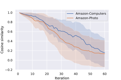
Figure 1. Average cosine similarity between the node embeddings of the original graph and the perturbed graph, results are on datasets Amazon-Computers and Amazon-Photo. The shaded area represents the standard deviation.

At the $30$-th iteration, with $0.97^{30}=40.10\%$ edges and features left, the average similarity of the positive samples are under $0.5$ on Amazon-Photo. At the $60$-th iteration, with $0.97^{60}=16.08\%$ edges and features left, the average similarity drops under $0.2$ on both Amazon-Computers and Amazon-Photo. Additionally, starting from the $30$-th iteration, the cosine similarity has around $0.3$ standard deviation for both datasets, which indicates that a lot of nodes are actually very sensitive to the external perturbations, even if we do not add any adversarial component but just mask out some information. These results demonstrate that the current graph contrastive learning framework is not trained over enough high-quality contrastive samples and is not robust to adversarial attacks.

Given this observation, we are motivated to build an adversarial graph contrastive learning framework that could improve the performance and robustness of the previous graph contrastive learning methods. The overview of our framework is shown in Figure 2.

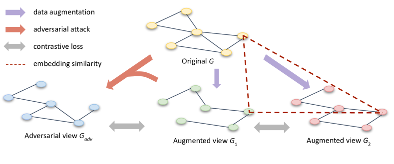
Figure 2. The overview of the proposed ArieL framework. For each iteration, two augmented views are generated from the original graph by data augmentation (purple arrows), and then an adversarial view is generated (red arrow) from the original graph by maximizing the contrastive loss against one of the augmented views. Besides, the similarities of the corresponding nodes (dashed lines) will get penalized by the information regularization if they exceed the estimated upper bound. The objective of ArieL is to minimize the contrastive loss (grey arrows) between the augmented views, the adversarial view, and the corresponding augmented view, and the information regularization. Best viewed in color.

3.2. Adversarial Training

Adversarial training uses the samples generated through the adversarial attack methods to improve the generalization ability and robustness of the original method during training. Although most existing attack frameworks are targeted at supervised learning, it is natural to generalize these methods to contrastive learning by replacing the classification loss with the contrastive loss. The goal of the adversarial attack on graph contrastive learning is to maximize the contrastive loss by adding a small perturbation on the contrastive samples, which can be formulated as

(11) $$G_{\text{adv}}=\arg\max_{G^{\prime}}L_{\text{con}}(G_{1},G^{\prime}),$$

where $G^{\prime}=\{\mathbf{A}^{\prime},\mathbf{X}^{\prime}\}$ is generated from the original graph $G$, and the change is constrained by the budget $\Delta_{\mathbf{A}}$ and $\Delta_{\mathbf{X}}$ as

(12) $$\sum_{i,j}|\mathbf{A}^{\prime}[i,j]-\mathbf{A}[i,j]|\leq\Delta_{\mathbf{A}},$$

(13) $$\sum_{i,j}|\mathbf{X}^{\prime}[i,j]-\mathbf{X}[i,j]|\leq\Delta_{\mathbf{X}}.$$

We treat adversarial attacks as one kind of data augmentation. Although we find it effective to make the adversarial attack on one or two augmented views as well, we follow the typical contrastive learning procedure as in SimCLR (Chen et al., 2020) to make the attack on the original graph in this work. Besides, it does not matter whether $G_{1}$, $G_{2}$ or $G$ is chosen as the anchor for the adversary, each choice works in our framework and it can also be sampled as a third view. In our experiments, we use PGD attack (Madry et al., 2019) as our attack method.

We generally follow the method proposed by Xu et al. (Xu et al., 2019) to make the PGD attack on the graph structure and apply the regular PGD attack method on the node features. Define the supplement of the adjacency matrix as $\mathbf{\bar{A}}=\mathbf{1}_{n\times n}-\mathbf{I}_{n}-\mathbf{A}$, where $\mathbf{1}_{n\times n}$ is the ones matrix of size $n\times n$. The perturbed adjacency matrix can be written as

(14) $$\mathbf{A}_{\text{adv}} =\mathbf{A}+\mathbf{C}\circ\mathbf{L}_{\mathbf{A}},$$

(15) $$\mathbf{C} =\bar{\mathbf{A}}-\mathbf{A},$$

where $\circ$ is the element-wise product, and $\mathbf{L}_{\mathbf{A}}\in\{0,1\}^{n\times n}$ is a symmetric matrix with each element $\mathbf{L}_{\mathbf{A}}[i,j]$ corresponding to the modification (e.g., add, delete or no modification) of the edge between the node pair $(v_{i},v_{j})$. The perturbation on $\mathbf{X}$ follows the regular PGD attack procedure and the perturbed feature matrix can be written as

(16) $$\mathbf{X}_{\text{adv}}=\mathbf{X}+\mathbf{L}_{\mathbf{X}},$$

where $\mathbf{L}_{\mathbf{X}}\in\mathbb{R}^{n\times d}$ is the perturbation on the feature matrix.

For the ease of optimization, $\mathbf{L}_{\mathbf{A}}$ is relaxed to its convex hull $\tilde{\mathbf{L}}_{\mathbf{A}}\in[0,1]^{n\times n}$, which satisfies $\mathcal{S}_{\mathbf{A}}=\{\tilde{\mathbf{L}}_{\mathbf{A}}|\sum\limits_{i,j}\tilde{\mathbf{L}}_{\mathbf{A}}\leq\Delta_{\mathbf{A}},\tilde{\mathbf{L}}_{\mathbf{A}}\in[0,1]^{n\times n}\}$. The constraint on $\mathbf{L}_{\mathbf{X}}$ can be written as $\mathcal{S}_{\mathbf{X}}=\{\mathbf{L}_{\mathbf{X}}|\|\mathbf{L}_{\mathbf{X}}\|_{\infty}\leq\delta_{\mathbf{X}},\mathbf{L}_{\mathbf{X}}\in\mathbb{R}^{n\times d}\}$, where we directly treat $\delta_{\mathbf{X}}$ as the constraint on the feature perturbation. In each iteration, we make the updates

(17) $$\tilde{\mathbf{L}}_{\mathbf{A}}^{(t)} =\Pi_{\mathcal{S}_{\mathbf{A}}}[\tilde{\mathbf{L}}_{\mathbf{A}}^{(t-1)}+\alpha\cdot\mathbf{G}_{\mathbf{A}}^{(t)}],$$

(18) $$\mathbf{L}_{\mathbf{X}}^{(t)} =\Pi_{\mathcal{S}_{\mathbf{X}}}[\mathbf{L}_{\mathbf{X}}^{(t-1)}+\beta\cdot\text{sgn}(\mathbf{G}_{\mathbf{X}}^{(t)})],$$

where $t$ denotes the current number of iterations, and

(19) $$\mathbf{G}_{\mathbf{A}}^{(t)} =\nabla_{\tilde{\mathbf{L}}_{\mathbf{A}}}L_{\text{con}}(G_{1},G_{\text{adv}}^{(t-1)}),$$

(20) $$\mathbf{G}_{\mathbf{X}}^{(t)} =\nabla_{\mathbf{L}_{\mathbf{X}}}L_{\text{con}}(G_{1},G_{\text{adv}}^{(t-1)}),$$

denote the gradients of the loss with respect to $\tilde{\mathbf{L}}_{\mathbf{A}}$ at $\tilde{\mathbf{L}}_{\mathbf{A}}^{(t-1)}$ and $\mathbf{L}_{\mathbf{X}}$ at $\mathbf{L}_{\mathbf{X}}^{(t-1)}$ respectively. Here $G_{\text{adv}}^{(t-1)}$ is defined as $\{\mathbf{A}+\mathbf{C}\circ\tilde{\mathbf{L}}_{\mathbf{A}}^{(t-1)},\mathbf{X}+\mathbf{L}_{\mathbf{X}}^{(t-1)}\}$. The projection operation $\Pi_{\mathcal{S}_{\mathbf{X}}}$ simply clips $\mathbf{L}_{\mathbf{X}}$ into the range $[-\delta_{\mathbf{X}},\delta_{\mathbf{X}}]$ elementwisely. The projection operation $\Pi_{\mathcal{S}_{\mathbf{A}}}$ is calculated as

(21) $$\Pi_{\mathcal{S}_{\mathbf{A}}}(\mathbf{Z})=\begin{cases}P_{[0,1]}[\mathbf{Z}-\mu\mathbf{1}_{n\times n}],&\text{if }\mu>0,\text{and }\sum\limits_{i,j}{P_{[0,1]}[\mathbf{Z}-\mu\mathbf{1}_{n\times n}]}=\Delta_{\mathbf{A}},\\ \\ P_{[0,1]}[\mathbf{Z}],&\text{if }\sum\limits_{i,j}{P_{[0,1]}[\mathbf{Z}]}\leq\Delta_{\mathbf{A}},\end{cases}$$

where $P_{[0,1]}[\mathbf{Z}]$ clips $\mathbf{Z}$ into the range $[0,1]$. We use the bisection method (Boyd and Vandenberghe, 2004) to solve the equation $\sum\limits_{i,j}P_{[0,1]}[\mathbf{Z}-\mu\mathbf{1}_{n\times n}]=\Delta_{\mathbf{A}}$ with respect to the dual variable $\mu$.

To finally obtain $\mathbf{L}_{\mathbf{A}}$ from $\tilde{\mathbf{L}}_{\mathbf{A}}$, each element is independently sampled from a Bernoulli distribution as $\mathbf{L}_{\mathbf{A}}[i,j]\sim\text{Bernoulli}(\tilde{\mathbf{L}}_{\mathbf{A}}[i,j])$. To obtain a symmetric matrix, we only sample the upper triangular part (the elements on the diagonal are known to be $0$ in our formulation) and obtain the lower triangular part through transposition.

3.3. Adversarial Graph Contrastive Learning

To assimilate the graph contrastive learning and adversarial training together, we treat the adversarial view $G_{\text{adv}}$ obtained from Equation (11) as another view of the graph. We define the adversarial contrastive loss as the contrastive loss between $G_{1}$ and $G_{\text{adv}}$. The adversarial contrastive loss is added to the original contrastive loss in Equation (3), which becomes

(22) $$L(G_{1},G_{2},G_{\text{adv}})=L_{\text{con}}(G_{1},G_{2})+\epsilon_{1}L_{\text{con}}(G_{1},G_{\text{adv}}),$$

where $\epsilon_{1}>0$ is the adversarial contrastive loss coefficient. We further adopt two additional subtleties on top of this basic framework: subgraph sampling and curriculum learning. For each iteration, a subgraph $G_{s}$ with a fixed size is first sampled from the original graph $G$, then the data augmentation and adversarial attack are both conducted on this subgraph. The subgraph sampling could avoid the gradient derivation on the whole graph, which will lead to heavy computation on a large network. Besides, we also observe that subgraph sampling could increase the randomness of the sample and sometimes boost the performance. To avoid the imbalanced sample on the isolated nodes, we uniformly sample a random set of nodes and then construct the subgraph atop them. For every $T$ epochs, the adversarial contrastive loss coefficient is multiplied by a weight $\gamma$. When $\gamma>1$, the portion of the adversarial contrastive loss is gradually increasing and the contrastive learning becomes harder as the training goes on.

3.4. Information Regularization

Adversarial training could effectively improve the model’s robustness to the perturbations, nonetheless, we find these hard training samples could impose the additional risk of training collapsing, i.e., the model will be located at a bad parameter area at the early stage of the training, assigning higher probability to a highly perturbed sample than a mildly perturbed one. In our experiment, we find this vanilla adversarial training method may fail to converge in some cases (e.g., Amazon-Photo dataset). To stabilize the training, we add one constraint termed information regularization, whose main goal is to regularize the instance similarity in the feature space.

The data processing inequality (Cover and Thomas, 2006) states that for three random variables $\mathbf{Z}_{1}$, $\mathbf{Z}_{2}$ and $\mathbf{Z}_{3}\in\mathbb{R}^{n\times d^{\prime}}$, if they satisfy the Markov relation $\mathbf{Z_{1}}\rightarrow\mathbf{Z}_{2}\rightarrow\mathbf{Z}_{3}$, then the inequality $I(\mathbf{Z}_{1};\mathbf{Z}_{3})\leq I(\mathbf{Z}_{1};\mathbf{Z}_{2})$ holds. As proved by Zhu et al. (Zhu et al., 2021), since the node embeddings of two views $\mathbf{H}_{1}$ and $\mathbf{H}_{2}$ are conditionally independent given the node embeddings of the original graph $\mathbf{H}$, they also satisfy the Markov relation with $\mathbf{H}_{1}\rightarrow\mathbf{H}\rightarrow\mathbf{H}_{2}$, and vice versa. Therefore, we can derive the following properties over their mutual information

(23) $$I(\mathbf{H}_{1};\mathbf{H}_{2}) \leq I(\mathbf{H};\mathbf{H}_{1}),$$

(24) $$I(\mathbf{H}_{1};\mathbf{H}_{2}) \leq I(\mathbf{H};\mathbf{H}_{2}).$$

In fact, this inequality holds on each node. A sketch of the proof is that the embedding of each node $v_{i}$ is determined by all the nodes from its $l$-hop neighborhood if an $l$-layer GNN is used as the encoder, and this subgraph composed of its $l$-hop neighborhood also satisfies the Markov relation. Therefore, we can derive the more strict inequalities

(25) $$I(\mathbf{H}_{1}[i,:];\mathbf{H}_{2}[i,:]) \leq I(\mathbf{H}[i,:];\mathbf{H}_{1}[i,:]),$$

(26) $$I(\mathbf{H}_{1}[i,:];\mathbf{H}_{2}[i,:]) \leq I(\mathbf{H}[i,:];\mathbf{H}_{2}[i,:]).$$

Since $-L_{\text{con}}(G_{1},G_{2})$ is only a lower bound of the mutual information, directly applying the above constraints is hard, we only consider the constraints on the density ratio. Using the Markov relation for each node, we give the following theorem:

Theorem 1.

For two graph views $G_{1}$ and $G_{2}$ independently transformed from the graph $G$, the density ratio of their node embeddings $\mathbf{H}_{1}$ and $\mathbf{H}_{2}$ should satisfy $g(\mathbf{H}_{2}[i,:],\mathbf{H}_{1}[i,:])\leq g(\mathbf{H}_{2}[i,:],\mathbf{H}[i,:])$ and $g(\mathbf{H}_{1}[i,:],\mathbf{H}_{2}[i,:])\leq g(\mathbf{H}_{1}[i,:],\mathbf{H}[i,:])$, where $\mathbf{H}$ is the node embeddings of the original graph.

Proof.

Following the Markov relation of each node, we get

(27) $$\begin{split}p(\mathbf{H}_{2}[i,:]|\mathbf{H}_{1}[i,:])&=p(\mathbf{H}_{2}[i,:]|\mathbf{H}[i,:])p(\mathbf{H}[i,:]|\mathbf{H}_{1}[i,:])\\ &\leq p(\mathbf{H}_{2}[i,:]|\mathbf{H}[i,:]),\end{split}$$

and consequently

(28) $$\frac{p(\mathbf{H}_{2}[i,:]|\mathbf{H}_{1}[i,:])}{p(\mathbf{H}_{2}[i,:])}\leq\frac{p(\mathbf{H}_{2}[i,:]|\mathbf{H}[i,:])}{p(\mathbf{H}_{2}[i,:])}.$$

Since $g(\mathbf{a},\mathbf{b})\propto\frac{p(\mathbf{a}|\mathbf{b})}{p(\mathbf{a})}$, we get $g(\mathbf{H}_{2}[i,:],\mathbf{H}_{1}[i,:])\leq g(\mathbf{H}_{2}[i,:],\mathbf{H}[i,:])$. A similar proof applies to the other inequality. ∎

Note that $g(\cdot,\cdot)$ is symmetric for the two inputs, we thus get two upper bounds for $g(\mathbf{H}_{1}[i,:],\mathbf{H}_{2}[i,:])$. According to the previous definition, $g(\mathbf{a},\mathbf{b})=e^{\theta(\mathbf{a},\mathbf{b})/\tau}$, we can simply replace $g(\cdot,\cdot)$ with $\theta(\cdot,\cdot)$ in the inequalities, then we combine these two upper bounds into one

(29) $$2\cdot\theta(\mathbf{H}_{1}[i,:],\mathbf{H}_{2}[i,:])\leq\theta(\mathbf{H}_{2}[i,:],\mathbf{H}[i,:])+\theta(\mathbf{H}_{1}[i,:],\mathbf{H}[i,:]).$$

This bound intuitively requires the similarity between $\mathbf{H}_{1}[i,:]$ and $\mathbf{H}_{2}[i,:]$ to be less than the similarity between $\mathbf{H}[i,:]$ and $\mathbf{H}_{1}[i,:]$ or $\mathbf{H}_{2}[i,:]$. Equipped with this upper bound, we define the following information regularization to penalize the higher probability of a less similar contrastive pair

(30) $$d_{i}=2\cdot\theta(\mathbf{H}_{1}[i,:],\mathbf{H}_{2}[i,:])-(\theta(\mathbf{H}_{2}[i,:],\mathbf{H}[i,:])+\theta(\mathbf{H}_{1}[i,:],\mathbf{H}[i,:])),$$

(31) $$L_{I}(G_{1},G_{2},G)=\frac{1}{n}\sum\limits_{i=1}^{n}{\max\{d_{i},0\}}.$$

Specifically, the information regularization could be defined over any three graphs that satisfy the Markov relation, but for our framework, to save the memory and time complexity, we avoid additional sampling and directly ground the information regularization on the existing graphs. It is also fine to apply the information regularization on $G$, $G_{1}$ and $G_{\text{adv}}$ or $G$, $G_{2}$ and $G_{\text{adv}}$.

The final loss of ArieL can be written as

(32) $$L(G_{1},G_{2},G_{\text{adv}})=L_{\text{con}}(G_{1},G_{2})+\epsilon_{1}L_{\text{con}}(G_{1},G_{\text{adv}})+\epsilon_{2}L_{I}(G_{1},G_{2},G),$$

where $\epsilon_{2}>0$ controls the strength of the information regularization.

The entire algorithm of ArieL is summarized in Algorithm 1.

Algorithm 1 Algorithm of ArieL

  Input data: Graph $G=(\mathbf{A},\mathbf{X})$

  Input parameters: $\alpha$, $\beta$, $\Delta_{\mathbf{A}}$, $\delta_{\mathbf{X}}$, $\epsilon_{1}$, $\epsilon_{2}$, $\gamma$ and $T$

  Randomly initialize the graph encoder $f$

  for iteration $k=0,1,\cdots$ do

     Sample a subgraph $G_{s}$ from $G$

     Generate two views $G_{1}$ and $G_{2}$ from $G_{s}$

     Generate the adversarial view $G_{\text{adv}}$ according to Equations (18) and (17)

     Update model $f$ to minimize $L(G_{1},G_{2},G_{\text{adv}})$ in Equation (32)

     if $(k+1)\mod T=0$ then

        Update $\epsilon_{1}\leftarrow\gamma*\epsilon_{1}$

     end if

  end for

  return: Node embedding matrix $\mathbf{H}=f(\mathbf{A},\mathbf{X})$

3.5. Extension to Graph-Level Contrastive Learning

For a batch of graphs $\mathcal{B}$ and the batch of their augmentation views $\mathcal{B}^{+}$, we aim to generate a batch of adversarial views, which we denote as $\mathcal{B}_{\text{adv}}$. Denote the combined graph of each batch as $G^{*}$, ${G^{+}}^{*}$ and $G_{\text{adv}}^{*}$. The objective of the adversarial graph contrastive learning on the graph level can be formulated as

(33) $$\mathcal{B}_{\text{adv}}=\arg \max_{\mathcal{B}^{\prime}}L_{\text{con}}(\mathcal{B}^{+},\mathcal{B}^{\prime}),$$

(34) subject to $$\sum_{i,j}|{\mathbf{A}^{\prime}}^{*}[i,j]-{\mathbf{A}}^{*}[i,j]|\leq\Delta_{\mathbf{A}},$$

(35) $$\sum_{i,j}|{\mathbf{X}^{\prime}}^{*}[i,j]-{\mathbf{X}}^{*}[i,j]|\leq\Delta_{\mathbf{X}}.$$

It is worth noting that the constraints we use here are applied on the batch rather than each graph, i.e., we only constrain the total perturbations over all graphs rather than the perturbations on each graph. This can greatly reduce the computational cost in solving the above-constrained maximization problem in that it reduces the number of constraints from twice the batch size to 2. However, it also introduces the additional risk that the perturbations could be severely imbalanced among the graphs in the batch, e.g., a graph is heavily perturbed while others are almost unchanged. In our experiment, we do not observe this problem but it could theoretically happen. A good practice is to start from this simple form, and then gradually add constraints to the vulnerable graphs in the batch if the imbalanced perturbations are observed.

During the attack stage, the perturbation matrix $\mathbf{L}_{\mathbf{A}}$ and its convex hull $\tilde{\mathbf{L}}_{\mathbf{A}}$ are further subject to the constraints that they should be block diagonal matrices with 0 at position $(i,j)$ if node $i$ and node $j$ are the nodes from two graphs in the batch. This could be easily implemented by using a block diagonal mask to zero out the gradients during the forward propagation,

(36) $$\mathbf{L}_{\mathbf{A}} =\text{block\_diag}(\mathbf{1}_{n_{i}\times n_{i}}|i=1\cdots,b)\circ\mathbf{L}_{\mathbf{A}},$$

(37) $$\tilde{\mathbf{L}}_{\mathbf{A}} =\text{block\_diag}(\mathbf{1}_{n_{i}\times n_{i}}|i=1\cdots,b)\circ\tilde{\mathbf{L}}_{\mathbf{A}},$$

where $n_{i}$ is the number of nodes in the graph $G_{i}$ in the batch. With this processing, the projection operation on the adjacency matrix remains the same as in Equation (21). In case we need to apply the constraints for each graph in the batch, we just need to apply the projection operation defined in Equation (21) on the adjacency matrix of each graph, using the bisection method to solve $\mu$ for each graph separately. The projection operation on the feature perturbation matrix is not affected on the graph level, which still clips $\mathbf{L}_{\mathbf{X}}$ into the range $[-\delta_{\mathbf{X}},\delta_{\mathbf{X}}]$ elementwisely.

Furthermore, the information regularization also applies to graph-level contrastive learning, where we only need to replace the node embedding with the graph embedding in Equation (30). Hence, we can derive the bound atop different views of the same graph in $\mathcal{B}$, $\mathcal{B}^{+}$ and $\mathcal{B}_{\text{adv}}$,

(38) $$d_{i}=2\cdot\theta(R(\mathbf{H}^{+}_{i}),R(\mathbf{H}_{\text{adv},i}))-(\theta(R(\mathbf{H}^{+}_{i}),R(\mathbf{H}_{i}))+\theta(R(\mathbf{H}_{\text{adv,i}}),R(\mathbf{H}_{i}))),$$

(39) $$L_{I}(\mathcal{B},\mathcal{B}^{+},\mathcal{B}_{\text{adv}})=\frac{1}{b}\sum\limits_{i=1}^{b}{\max\{d_{i},0\}}.$$

The final loss of ArieL for the graph-level contrastive learning could be written as

(40) $$L(\mathcal{B},\mathcal{B}^{+},\mathcal{B}_{\text{adv}})=L_{\text{con}}(\mathcal{B},\mathcal{B}^{+})+\epsilon_{1}L_{\text{con}}(\mathcal{B}^{+},\mathcal{B}_{\text{adv}})+\epsilon_{2}L_{I}(\mathcal{B},\mathcal{B}^{+},\mathcal{B}_{\text{adv}}).$$

The graph-level adversarial contrastive learning could also follow the steps outlined in Algorithm 1 for training, by simply replacing the input graph with the input batch in loss functions.

4. Experiments

In this section, we conduct empirical evaluations, which are designed to answer the following three questions:

• How effective is the proposed ArieL in comparison with previous graph contrastive learning methods on the node classification and graph classification task?

• To what extent does ArieL gain robustness over the attacked graph?

• How does each part of ArieL contribute to its performance?

We evaluate our method with the node classification task and graph classification task on the real-world graphs and further evaluate the robustness of it with the node classification task on the attacked graphs. The node/graph embeddings are first learned by the proposed ArieL algorithm, then the embeddings are fixed to perform the classification with a simple classifier trained over it. All our experiments are conducted on the NVIDIA Tesla V100S GPU with 32G memory.

4.1. Experimental Setup

4.1.1. Datasets

For the node-level contrastive learning, we use eight datasets for the evaluation, including Cora, CiteSeer, Amazon-Computers, Amazon-Photo, Coauthor-CS, Coauthor-Physics, Facebook and LastFM Asia. Cora and CiteSeer (Yang et al., 2016) are citation networks, where nodes represent documents and edges correspond to citations. Amazon-Computers and Amazon-Photo (Shchur et al., 2019) are extracted from the Amazon co-purchase graph. In these graphs, nodes are the goods and they are connected by an edge if they are frequently bought together. Coauthor-CS and Coauthor-Physics (Shchur et al., 2019) are the co-authorship graphs, where each node is an author and the edge indicates the co-authorship on a paper. Facebook (Rozemberczki et al., 2019) is a page-page graph of verified Facebook pages where edges correspond to the likes of each other. LastFM Asia (Rozemberczki and Sarkar, 2020) is a social network of Asian users, each node represents a user and they are connected via friendship.

For the graph-level contrastive learning, we evaluate ArieL on four datasets from the benchmark TUDataset (Morris et al., 2020), including the biochemical molecules graphs NCI1, PROTEINS, DD and MUTAG.

A summary of the datasets statistics is in Table 1 and Table 2.

Dataset	Nodes	Edges	Features	Classes
Cora	2,708	5,429	1,433	7
CiteSeer	3,327	4,732	3,703	6
Amazon-Computers	13,752	245,861	767	10
Amazon-Photo	7,650	119,081	745	8
Coauthor-CS	18,333	81,894	6,805	15
Coauthor-Physics	34,493	247,962	8,415	5
Facebook	22,470	342,004	128	4
LastFM Asia	7,624	55,612	128	18

Table 1. Node-level contrastive learning datasets statistics, the number of nodes, edges, node feature dimensions, and classes are listed.

Dataset	Graphs	Nodes	Degree	Features	Classes
NCI1	4110	29.87	1.08	37	2
PROTEINS	1113	39.06	1.86	3	2
DD	1178	284.32	2.52	89	2
MUTAG	188	17.93	1.10	7	2

Table 2. Graph-level contrastive learning datasets statistics, number of graphs, the average number of nodes and degree, and the number of node feature dimensions and classes are listed.

4.1.2. Baselines

We consider seven graph contrastive learning methods for node-level contrastive learning, including DeepWalk (Perozzi et al., 2014), DGI (Veličković et al., 2018b), Robust DGI (abbreviated as RDGI) (Xu et al., 2020), GMI (Peng et al., 2020), MVGRL (Hassani and Khasahmadi, 2020), GRACE (Zhu et al., 2020) and GCA (Zhu et al., 2021). Since DeepWalk only generates the embeddings for the graph topology, we concatenate the node features to the generated embeddings for evaluation so that the final embeddings can incorporate both topology and attribute information. Besides, we also compare our method with two supervised methods Graph Convolutional Network (GCN) (Kipf and Welling, 2017) and Graph Attention Network (GAT) (Veličković et al., 2018a).

For graph-level contrastive learning, we compare ArieL with the state-of-the-art graph kernel methods including graphlet kernel (GL), Weisfeiler-Lehman sub-tree kernel (WL) and deep graph kernel (DGK), and recent unsupervised graph representation learning methods including node2vec (Grover and Leskovec, 2016), sub2vec (Adhikari et al., 2018), graph2vec (Narayanan et al., 2017), InfoGraph (Sun et al., 2019) and GraphCL (You et al., 2020).

4.1.3. Evaluation protocol

For each dataset, we randomly select $10\%$ nodes/graphs for training, $10\%$ nodes/graphs for validation, and the remaining for testing. For contrastive learning methods, a logistic regression classifier is trained to do the node classification over the node embeddings while a support vector machine is trained to do the graph classification over the graph embeddings. The accuracy is used as the evaluation metric.

For node-level contrastive learning, we search each method over $6$ different random seeds, including $5$ random seeds from our own and the best random seed of GCA on each dataset. For each seed, we evaluate the method on $20$ random training-validation-testing dataset splits and report the mean and the standard deviation of the accuracy on the best seed. Specifically, for the supervised learning methods, we abandon the existing splits, for example on Cora and CiteSeer, but instead do a random split before the training and report the results over $20$ splits.

For graph-level contrastive learning, we keep the evaluation protocol the same as the setting in (Sun et al., 2019) and (You et al., 2020), where the experiments are conducted on 5 random seeds, each corresponding to a 10-fold evaluation.

Besides testing on the original, clean graphs, we also evaluate our method on the attacked graphs for node-level contrastive learning. We use Metattack (Zügner and Günnemann, 2019) to perform the poisoning attack. Since Metattack is targeted at graph structure only and computationally inefficient on large graphs, we first randomly sample a subgraph of $5000$ nodes if the number of nodes in the original graph is greater than $5000$, then we randomly mask out $20\%$ node features and finally use Metattack to perturb $20\%$ edges to generate the final attacked graph. For ArieL, we use the hyperparameters of the best models we obtain on the clean graphs for evaluation. For GCA, we report the performance in our main results for its three variants, GCA-DE, GCA-PR, and GCA-EV, which correspond to the adoption of degree, eigenvector, and PageRank (Page et al., 1999; Kang et al., 2018) centrality measures, and use the best variant on each dataset for the evaluation on the attacked graphs.

4.2. Hyperparameters

For node-level contrastive learning, we use the same parameters and design choices for ArieL’s network architecture, optimizer and training scheme as in GRACE and GCA on each dataset. However, we find GCA not behave well on Cora with a significant performance drop, so we re-search the parameters for GCA on Cora separately and use a different temperature for it. Other contrastive learning-specific parameters are kept the same over GRACE, GCA and ArieL. On graph-level contrastive learning, we keep ArieL’s hyperparameters the same as the ones used by GraphCL except for its own parameters.

All GNN-based baselines on node-contrastive learning use a two-layer GCN as the encoder. For each method, we compare its default hyperparameters and the ones used by ArieL and use the hyperparameters leading to better performance. Other algorithm-specific hyperparameters all respect the default setting in its official implementation. For graph-level contrastive learning, ArieL uses a three-layer GIN as the encoder, and we take the results for each baseline from its original paper under the same experimental setting.

Other hyperparameters of ArieL are summarized as follows:

• Adversarial contrastive loss coefficient $\epsilon_{1}$ and information regularization strength $\epsilon_{2}$. We search them over $\{0.5,1,1.5,2\}$ and use the one with the best performance on the validation set of each dataset. Specifically, we first fix $\epsilon_{2}$ as $0$ and decide the optimal value for all other parameters, then we search $\epsilon_{2}$ on top of the model with other hyperparameters fixed.

• Number of attack steps and perturbation constraints. These parameters are fixed on all datasets. For node-level contrastive learning, we set the number of attack steps 5, edge perturbation constraint $\Delta_{\mathbf{A}}=0.1\sum_{i,j}\mathbf{A}[i,j]$ and feature perturbation constraint $\delta_{\mathbf{X}}=0.5$. For graph-level contrastive learning, we set the number of attack steps 5, edge perturbation constraint $\Delta_{\mathbf{A}}=0.05\sum_{i,j}\mathbf{A}[i,j]$ and feature perturbation constraint $\delta_{\mathbf{X}}=0.04$.

• Curriculum learning weight $\gamma$ and change period $T$. In our experiments, we simply fix $\gamma=1.1$ and $T=20$ for node-level contrastive learning and $\gamma=1$ for graph-level contrastive learning.

• Graph perturbation rate $\alpha$ and feature perturbation rate $\beta$. We search both of them over $\{0.001,0.01,0.1\}$ and take the best one on the validation set of each dataset.

• Subgraph size. On node-level contrastive learning, we keep the subgraph size $500$ for ArieL on all datasets except Facebook and LastFM Asia, where we use a subgraph size $3000$. We do not do the subgraph sampling on graph-level contrastive learning. Instead, we control the batch size $b$, where we fix $b=32$ for DD and $b=128$ for the other three datasets.

4.3. Main Results

The comparison results of node classification on all eight datasets are summarized in Table 3. Our method ArieL outperforms baselines over all datasets except on Cora and Facebook, with only $0.11\%$ and $0.40\%$ lower in accuracy than MVGRL. It can be seen that the previous state-of-the-art method GCA does not bear significant improvements over previous methods. In contrast, ArieL can achieve consistent improvements over GRACE and GCA on all datasets, especially on Amazon-Computers with almost $3\%$ gain.

Method	Cora	CiteSeer	Amazon- Computers	Amazon- Photo	Coauthor- CS	Coauthor- Physics	Facebook	LastFM Asia
GCN	$84.14\pm 0.68$	$69.02\pm 0.94$	$88.03\pm 1.41$	$92.65\pm 0.71$	$92.77\pm 0.19$	$95.76\pm 0.11$	89.98 $\pm$ 0.26	83.96 $\pm$ 0.47
GAT	$83.18\pm 1.17$	$69.48\pm 1.04$	$85.52\pm 2.05$	$91.35\pm 1.70$	$90.47\pm 0.35$	$94.82\pm 0.21$	89.97 $\pm$ 0.39	83.04 $\pm$ 0.39
DeepWalk	$79.82\pm 0.85$	$67.14\pm 0.81$	$86.23\pm 0.37$	$90.45\pm 0.45$	$85.02\pm 0.44$	$94.57\pm 0.20$	86.67 $\pm$ 0.22	83.93 $\pm$ 0.61
DGI	$84.24\pm 0.75$	$69.12\pm 1.29$	$88.78\pm 0.43$	$92.57\pm 0.23$	$92.26\pm 0.12$	$95.38\pm 0.07$	89.80 $\pm$ 0.27	82.88 $\pm$ 0.52
RDGI	$81.84\pm 1.07$	$65.92\pm 1.26$	$88.07\pm 0.28$	$92.17\pm 0.27$	OOM	OOM	OOM	$77.34\pm 0.69$
GMI	$82.43\pm 0.90$	$70.14\pm 1.00$	$83.57\pm 0.40$	$88.04\pm 0.59$	OOM	OOM	OOM	74.71 $\pm$ 0.70
MVGRL	84.39 $\pm$ 0.77	$69.85\pm 1.54$	$89.02\pm 0.21$	$92.92\pm 0.25$	$92.22\pm 0.22$	$95.49\pm 0.17$	90.60 $\pm$ 0.28	83.83 $\pm$ 0.85
GRACE	$83.40\pm 1.08$	$69.47\pm 1.36$	$87.77\pm 0.34$	$92.62\pm 0.25$	$93.06\pm 0.08$	$95.64\pm 0.08$	88.95 $\pm$ 0.31	79.52 $\pm$ 0.64
GCA-DE	$82.57\pm 0.87$	$72.11\pm 0.98$	$88.10\pm 0.33$	$92.87\pm 0.27$	$93.08\pm 0.18$	$95.62\pm 0.13$	89.73 $\pm$ 0.37	82.42 $\pm$ 0.46
GCA-PR	$82.54\pm 0.87$	$72.16\pm 0.73$	$88.18\pm 0.39$	$92.85\pm 0.34$	$93.09\pm 0.15$	$95.58\pm 0.12$	89.68 $\pm$ 0.36	82.44 $\pm$ 0.51
GCA-EV	$81.80\pm 0.92$	$67.07\pm 0.79$	$87.95\pm 0.43$	$92.63\pm 0.33$	$93.06\pm 0.14$	$95.64\pm 0.08$	89.68 $\pm$ 0.38	82.35 $\pm$ 0.46
ARIEL	84.28 $\pm$ 0.96	72.74 $\pm$ 1.10	91.13 $\pm$ 0.34	94.01 $\pm$ 0.23	93.83 $\pm$ 0.14	95.98 $\pm$ 0.05	90.20$\pm$ 0.23	84.04$\pm$0.44

Table 3. Node classification accuracy in percentage on eight real-world datasets. We bold the results with the best mean accuracy. The methods above the line are the supervised ones, and the ones below the line are unsupervised. OOM stands for Out-of-Memory on our 32G GPUs.

Besides, we find MVGRL a solid baseline whose performance is close to or even better than GCA on these datasets. It achieves the highest score on Cora and Facebook, and the second-highest on Amazon-Computers and Amazon-Photo. However, it does not behave well on CiteSeer, where GCA can effectively increase the score of GRACE. To sum up, previous modifications over the grounded frameworks are mostly based on specific knowledge, for example, MVGRL introduces the diffusion matrix to DGI and GCA defines the importance on the edges and features, and they cannot consistently take effect on all datasets. However, ArieL uses the adversarial attack to automatically construct the high-quality contrastive samples and achieves more stable performance improvements.

In comparison with the supervised methods, ArieL also achieves a clear advantage over all of them. Although it would be premature to conclude that ArieL is more powerful than these supervised methods since they are usually tested under the specific training-testing split, these results do demonstrate that ArieL can indeed generate highly expressive node embeddings for the node classification task, which can achieve comparable performance to the supervised methods.

The graph classification results are summarized in Table 4.

Method	NCI1	PROTEINS	DD	MUTAG
GL	-	-	-	81.66 $\pm$ 2.11
WL	80.11 $\pm$ 0.50	72.92 $\pm$ 0.56	-	80.72 $\pm$ 3.00
DGK	80.31 $\pm$ 0.46	73.30 $\pm$ 0.82	-	87.44 $\pm$ 2.72
node2vec	54.89 $\pm$ 1.61	57.49 $\pm$ 3.57	-	72.63 $\pm$ 10.20
sub2vec	52.84 $\pm$ 1.47	53.03 $\pm$ 5.55	-	61.05 $\pm$ 15.80
graph2vec	73.22 $\pm$ 1.81	73.30 $\pm$ 2.05	-	83.15 $\pm$ 9.25
InfoGraph	76.20 $\pm$ 1.06	74.44 $\pm$ 0.31	72.85 $\pm$ 1.78	89.01 $\pm$ 1.13
GraphCL	77.87 $\pm$ 0.41	74.39 $\pm$ 0.45	78.62 $\pm$ 0.40	86.80 $\pm$ 1.34
ARIEL	78.91 $\pm$ 0.36	75.22 $\pm$ 0.26	79.15 $\pm$ 0.53	89.25 $\pm$ 1.18

Table 4. Graph classification accuracy in percentage on four real-world datasets. We bold the results with the best mean accuracy. The methods above the double line belong to the graph kernel methods, and the ones below the double line are unsupervised representation learning methods. The compared numbers are from the original paper under the same experimental setting.

Compared with our basic framework GraphCL, which uses naive augmentation methods, ArieL achieves even stronger performance on all datasets. GraphCL does not show a clear advantage against previous baselines such as InfoGraph and it does not behave well on the dataset with small graph size (e.g., NCI1 and MUTAG). However, ArieL can take the lead on three of the datasets and greatly reduce the performance gap on NCI1 with the graph kernel methods. It can be clearly seen that ArieL behaves better than GraphCL on NCI1 and MUTAG with at least $1\%$ improvement in accuracy. In comparison with another graph contrastive learning method InfoGraph, we can also see that ArieL takes an overall lead on all datasets, even on MUTAG where InfoGraph shows a dominant advantage against other baselines.

The above empirical results on the node classification and graph classification tasks clearly demonstrate the advantage of ArieL on real-world graphs, which indicates the better augmentation strategy of ArieL.

4.4. Results under Attack

The results on attacked graphs are summarized in Table 5. Specifically, we evaluate all these methods on the attacked subgraph of Amazon-Computers, Amazon-Photo, Coauthor-CS, Coauthor-Physics, Facebook, and LastFM Asia, so their results are not directly comparable to the results in Table 3. To compare with the previous results, we look at the datasets where ArieL takes the lead, and then find the performance of the second-best method on each dataset for both the original graph and the attacked one. If ArieL outperforms the second-best method by a much larger margin on the attacked graph compared with that on the original graph, we claim that ArieL is significantly robust on that dataset.

Method	Cora	CiteSeer	Amazon- Computers	Amazon- Photo	Coauthor- CS	Coauthor- Physics	Facebook	LastFM Asia
GCN	$80.03\pm 0.91$	$62.98\pm 1.20$	$84.10\pm 1.05$	$91.72\pm 0.94$	$80.32\pm 0.59$	$87.47\pm 0.38$	70.07 $\pm$ 0.74	73.22 $\pm$ 0.85
GAT	$79.49\pm 1.29$	$63.30\pm 1.11$	$81.60\pm 1.59$	$90.66\pm 1.62$	$77.75\pm 0.80$	$86.65\pm 0.41$	72.02 $\pm$ 0.78	73.21 $\pm$ 0.64
DeepWalk	$74.12\pm 1.02$	$63.20\pm 0.80$	$79.08\pm 0.67$	$88.06\pm 0.41$	$49.30\pm 1.23$	$79.26\pm 1.38$	59.07 $\pm$ 1.01	67.61 $\pm$ 0.80
DGI	$80.84\pm 0.82$	$64.25\pm 0.96$	$83.36\pm 0.55$	$91.27\pm 0.29$	$78.73\pm 0.50$	$85.88\pm 0.37$	70.52 $\pm$ 0.93	71.80 $\pm$ 0.59
RDGI	$77.29\pm 1.01$	$59.94\pm 1.29$	$82.35\pm 0.59$	$90.63\pm 0.41$	$83.09\pm 0.64$	$83.58\pm 0.75$	$67.85\pm 1.19$	$63.59\pm 0.91$
GMI	79.17 $\pm$ 0.76	$65.37\pm 1.03$	$77.42\pm 0.59$	$89.44\pm 0.47$	$80.92\pm 0.64$	$87.72\pm 0.45$	68.93 $\pm$ 0.83	58.89 $\pm$ 0.95
MVGRL	80.90 $\pm$ 0.75	$64.81\pm 1.53$	$83.76\pm 0.69$	$91.76\pm 0.44$	$79.49\pm 0.75$	$86.98\pm 0.61$	71.76 $\pm$ 0.69	73.42 $\pm$ 1.11
GRACE	$78.55\pm 0.81$	$63.17\pm 1.81$	$84.74\pm 1.13$	$91.26\pm 0.37$	$80.61\pm 0.63$	$85.71\pm 0.38$	71.97 $\pm$ 0.98	69.39 $\pm$ 0.63
GCA	$76.79\pm 0.97$	$64.89\pm 1.33$	$85.05\pm 0.51$	$91.71\pm 0.34$	$82.72\pm 0.58$	$89.00\pm 0.31$	69.54 $\pm$ 0.82	71.83 $\pm$ 1.03
ARIEL	80.33 $\pm$ 1.25	69.13 $\pm$ 0.94	88.61 $\pm$ 0.46	92.99 $\pm$ 0.21	84.43 $\pm$ 0.59	89.09 $\pm$ 0.31	71.15 $\pm$ 1.19	73.94 $\pm$ 0.78

Table 5. Node classification accuracy in percentage on the graphs under Metattack, where subgraphs of Amazon-Computers, Amazon-Photo, Coauthor-CS and Coauthor-Physics, Facebook and LastFM Asia are used for attack and their results are not directly comparable to those in Table 3. We bold the results with the best mean accuracy. GCA is evaluated on its best variant on each clean graph.

Under this principle, we can see that ArieL is significantly robust on CiteSeer, with the margin to the second best method increasing from $0.58\%$ to $3.96\%$, Amazon-Computers, with the margin increasing from $2.11\%$ to $3.56\%$, and Coauthor-CS, with the margin increasing from $0.74\%$ to $1.71\%$. On Coauthor-Physics, ArieL and GCA both show clear robustness against the remaining methods. Although some baselines are robust on specific datasets, for example, MVGRL on Cora, GMI on CiteSeer, GCN on Facebook, and GCA on Coauthor-CS and Coauthor-Physics, they fail to achieve consistent robustness over all datasets. Although GCA indeed makes GRACE more robust for most datasets, it is still vulnerable on Cora, CiteSeer, and Amazon-Computers, with more than $3\%$ lower than ArieL in the final accuracy.

Besides, we can also see that ArieL still shows high robustness on the datasets where it cannot take the lead. On Cora and Facebook, ArieL is only less than $1\%$ lower in accuracy than the best method and it is still better than most baselines. It does not show a sudden performance drop on any dataset, such as MVGRL on CiteSeer and GCA on Facebook.

Basically, MVGRL and GCA can improve the robustness of their respective grounded frameworks over specific datasets, but we find this kind of improvement relatively minor. Instead, ArieL has more significant improvements and greatly increases robustness. It is worth noting that though RDGI is also developed to improve the robustness of graph representation learning, it does not show a clear advantage against DGI in our evaluation. This is mainly because the original RDGI considers the attack at test time and what we evaluate is the robustness against the attack at training time, which is more common for the graph learning tasks (Bojchevski and Günnemann, 2019; Zügner et al., 2018; Zügner and Günnemann, 2019). Based on the comparative results, we claim that ArieL is more robust than previous graph contrastive learning methods in the face of the adversarial attack.

4.5. Ablation Study

For this section, we first set $\epsilon_{2}$ as $0$ and investigate the role of adversarial contrastive loss. The adversarial contrastive loss coefficient $\epsilon_{1}$ controls the portion of the adversarial contrastive loss in the final loss. When $\epsilon_{1}=0$, the final loss reduces to the regular contrastive loss in Equation (3). To explore the effect of the adversarial contrastive loss, we fix other parameters in our best models on Cora and CiteSeer and gradually increase $\epsilon_{1}$ from $0$ to $2$. The changes in the final performance are shown in Figure 3.

The dashed line represents the performance of GRACE with subgraph sampling, i.e., $\epsilon_{1}=0$. Although there exist some variations, ArieL is always above the baseline under a positive $\epsilon_{1}$ with around $2\%$ improvement. The subgraph sampling trick may sometimes help the model, for example, it improves GRACE without subgraph sampling by $1\%$ on CiteSeer, but it could be detrimental as well, such as on Cora. This is understandable since subgraph sampling can simultaneously enrich the data augmentation and lessen the number of negative samples, both critical to contrastive learning. While for the adversarial contrastive loss, it has a stable and significant improvement on GRACE with subgraph sampling, which demonstrates that the performance improvement of ArieL mainly stems from the adversarial loss rather than the subgraph sampling.

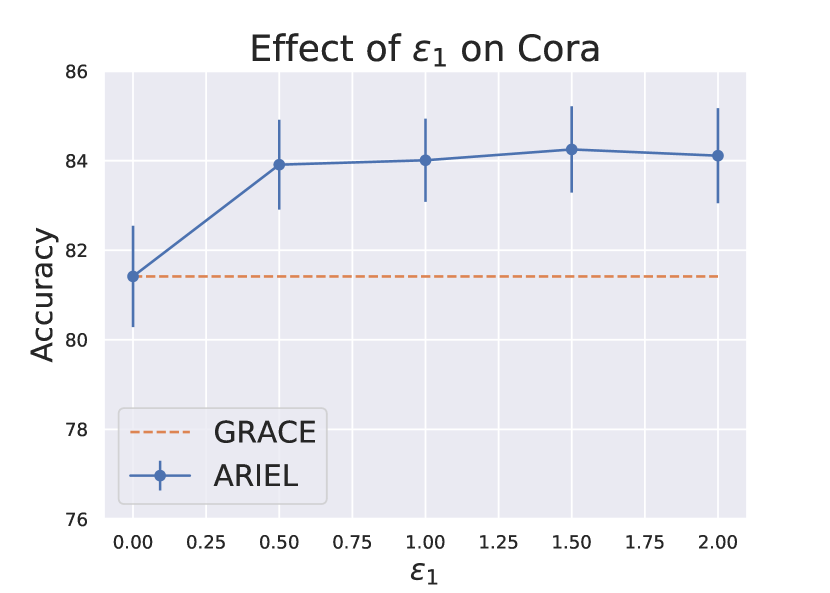
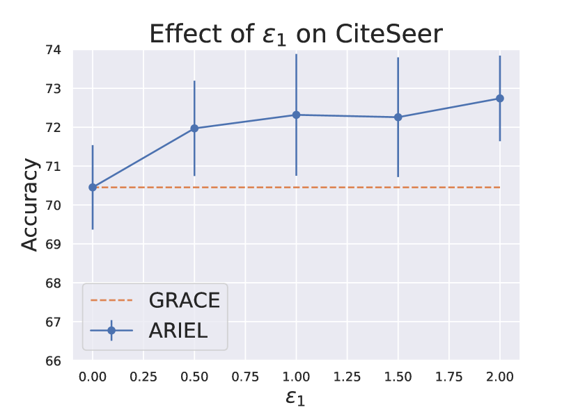
Figure 3. Effect of adversarial contrastive loss coefficient $\epsilon_{1}$ on Cora and CiteSeer. The dashed line represents the performance of GRACE with subgraph sampling.

Next, we fix all other parameters and check the behavior of $\epsilon_{2}$. Information regularization is mainly designed to stabilize the training of ArieL. We find ArieL would experience the collapsing at the early training stage and the information regularization could mitigate this issue. We choose the best run on Amazon-Photo, where the collapsing frequently occurs, and similar to before, we gradually increase $\epsilon_{2}$ from $0$ to $2$, the results are shown in Figure 4 (left).

Figure 4. Effect of information regularization on Amazon-Photo. The left figure shows the model performance under different $\epsilon_{2}$ and the right figure plots the training curve of ArieL under $\epsilon_{2}=0$ and $\epsilon_{2}=1.0$.

As can be seen, without using the information regularization, ArieL could collapse without learning anything, while setting $\epsilon_{2}$ greater than $0$ can effectively avoid this situation. To further illustrate this, we draw the training curve of the regular contrastive loss in Figure 4 (right), for the best ArieL model on Amazon-Photo and the same model by simply removing the information regularization. Without information regularization, the model could get stuck in a bad parameter area and fail to converge, while information regularization can resolve this issue.

4.6. Training Analysis

Here we compare the training of ArieL on node-level contrastive learning to other methods on our NVIDIA Tesla V100S GPU with 32G memory.

Adversarial attacks on graphs tend to be highly computationally expensive since the attack requires the gradient calculation over the entire adjacency matrix, which is of size $O(n^{2})$. For ArieL, we resolve this bottleneck with subgraph sampling on large graphs and empirically show that the adversarial training on the subgraph still yields significant improvements, without increasing the number of training iterations. In our experiments, we find GMI the most memory inefficient, which cannot be trained on Coauthor-CS, Coauthor-Physics, and Facebook. For DGI, MVGRL, GRACE, and GCA, the training of them also amounts to $30$G GPU memory on Coauthor-Physics while the training of ArieL requires no more than $8$G GPU memory. In terms of the training time, DGI and MVGRL are the fastest to converge, but it takes MVGRL a long time to compute the diffusion matrix on large graphs. ArieL is slower than GRACE and GCA on Cora and CiteSeer, but it is faster on large graphs like Coauthor-CS and Coauthor-Physics, with the training time for each iteration invariant to the graph size due to the subgraph sampling. On the largest graph Coauthor-Physics, each iteration takes GRACE 0.875 second and GCA 1.264 seconds, while it only takes ArieL 0.082 second. This demonstrates that ArieL has even better scalability than GRACE and GCA.

Subgraph sampling, under some mild assumptions, could be an efficient way to reduce the computational cost for any node-level contrastive learning algorithm. Besides this general trick, we want to point out that the attack is in fact not always needed on the whole graph to generate the adversarial view. Another solution to avoid explosive memory is to select some anchor nodes and only perturb the edges among these anchor nodes and their features. Since the scalability issue has been resolved by subgraph sampling on all datasets appearing in this work, we will not further discuss the details of this method and empirically prove its effectiveness, but leave it for future work.

5. Related Work

In this section, we review the related work in the following three categories: graph contrastive learning, adversarial attack on graphs, and adversarial contrastive learning.

5.1. Graph Contrastive Learning

Contrastive learning is known for its simplicity and strong expressivity. Traditional methods ground the contrastive samples on the node proximity in the graph, such as DeepWalk (Perozzi et al., 2014) and node2vec (Grover and Leskovec, 2016), which use random walks to generate the node sequences and approximate the co-occurrence probability of node pairs. However, these methods can only learn the embeddings for the graph structures but regardless of the node features.

GNNs (Kipf and Welling, 2017; Veličković et al., 2018a) can easily capture the local proximity and node features (Veličković et al., 2018b; Zhao et al., 2020; You et al., 2020; Jing et al., 2021e, c). To further improve the performance, the Information Maximization (InfoMax) principle (Linsker, 1988) has been introduced. DGI (Veličković et al., 2018b) is adapted from Deep InfoMax (Hjelm et al., 2019) to maximize the mutual information between the local and global features. It generates the negative samples with a corrupted graph and contrasts the node embeddings with the original graph embedding and the corrupted one. Based on a similar idea, GMI (Peng et al., 2020) generalizes the concept of mutual information to the graph domain by separately defining the mutual information on the features and edges. Graph Community Infomax (GCI) (Sun et al., 2021) instead tries to maximize the mutual information between the community representation and the node representation for those positive pairs. Another follow-up work of DGI, MVGRL (Hassani and Khasahmadi, 2020), maximizes the mutual information between the first-order neighbors and graph-diffusion. On the graph level, InfoGraph (Sun et al., 2019) makes use of a similar idea to maximize the mutual information between the global representation and patch representation from the same graph. HDI (Jing et al., 2021b) introduces high-order mutual information to consider both intrinsic and extrinsic training signals. However, mutual information-based methods generate the corrupted graphs by simply randomly shuffling the node features. Recent methods exploit the graph topology and features to generate better-augmented graphs. GCC (Qiu et al., 2020) adopts a random-walk-based strategy to generate different views of the context graph for a node, but it ignores the augmentation on the feature level. GCA (Zhu et al., 2020), instead, considers the data augmentation from both the topology and feature level, and introduces the adaptive augmentation by considering the importance of each edge and feature dimension. To investigate the power of different data augmentations in graph domains, GraphCL (You et al., 2020) systematically studies the different combinations of graph augmentation strategies and applies them to different graph learning settings. Unlike the above methods which construct the data augmentation samples based on domain knowledge, ArieL uses an adversarial attack to construct the view that maximizes the contrastive loss, which is more informative with broader applicability.

5.2. Adversarial Attack on Graphs

Deep learning methods are known vulnerable to adversarial attacks, and this is also the case in the graph domain. As shown by Bojchevski et al. (Bojchevski and Günnemann, 2019), both random-walk-based methods and GNNs-based methods could be attacked by flipping a small portion of edges. Xu et al. (Xu et al., 2019) propose a PGD attack and min-max attack on the graph structure from the optimization perspective. NETTACK (Zügner et al., 2018) is the first to attack GNNs using both structure attack and feature attack, causing a significant performance drop of GNNs on the benchmarks. After that, Metattack (Zügner and Günnemann, 2019) formulates the poisoning attack of GNNs as a meta-learning problem and achieves remarkable performance by only perturbing the graph structure. Node Injection Poisoning Attacks (Sun et al., 2020) uses a hierarchical reinforcement learning approach to sequentially manipulate the labels and links of the injected nodes. Recently, InfMax (Ma et al., 2021) formulated the adversarial attack on GNNs as an influence maximization problem.

5.3. Adversarial Contrastive Learning

The concept of adversarial contrastive learning is first proposed on visual domains (Kim et al., 2020; Jiang et al., 2020; Ho and Vasconcelos, 2020). All these works propose a similar idea to use the adversarial sample as a form of data augmentation in contrastive learning and it can bring better downstream task performance and higher robustness. ACL (Kim et al., 2020) studies the different paradigms of adversarial contrastive learning, by replacing one or two of the augmentation views with the adversarial view generated by PGD attack (Madry et al., 2019). CLAE (Ho and Vasconcelos, 2020) and RoCL (Jiang et al., 2020) use FGSM (Goodfellow et al., 2015) to generate an additional adversarial view atop the two standard augmentation views. RDGI (Xu et al., 2020) and AD-GCL (Suresh et al., 2021) are the most relevant work to ours in graph domains. RDGI quantifies the robustness of node representation as the decrease in mutual information between the graph and its embedding under adversarial attacks. It learns a robust node representation by simultaneously minimizing the standard contrastive learning loss and improving the robustness. Nonetheless, its objective sacrifices the expressiveness of the node representation for robustness while ArieL can improve both of them. AD-GCL formulates adversarial graph contrastive learning in a min-max form and uses a parameterized network for edge dropping. However, AD-GCL is designed for the graph classification task only and does not explore the robustness of graph contrastive learning. Finally, All previous adversarial contrastive learning methods do not take scalability into consideration, with visual models and AD-GCL dealing with independent instances and RDGI only working on small graphs, but ArieL can work for both interconnected instances (node embedding) and independent instances (graph embedding) on a large scale.

Some recent theoretical analyses further reveal the vulnerability of contrastive learning. Jing et al. (Jing et al., 2021d) show that dimensional collapse could happen if the variation of the data augmentation exceeds the variation of the data itself in contrastive learning. Wang et al. (Wang et al., 2022) prove that contrastive learning could cluster the instances from the same class only when the support of different intra-class samples overlaps under data augmentation. The representations learned by contrastive learning may fail in downstream tasks when either under-overlapping or overly overlapping happens. From these perspectives, searching for adversarial contrastive samples in a safe area is more likely to generate useful representations for downstream tasks.

6. Conclusion

In this paper, we propose a universal framework for graph contrastive learning by introducing an adversarial view, scaling it through subgraph sampling, and stabilizing it through information regularization. It consistently outperforms the state-of-the-art graph contrastive learning methods in the node classification and graph classification tasks and exhibits a higher degree of robustness to the adversarial attack. Our framework is not limited to the graph contrastive learning frameworks we build on in this paper, and it can be naturally extended to other graph contrastive learning methods as well. In the future, we plan to further investigate (1) the adversarial attack on graph contrastive learning and (2) the integration of graph contrastive learning and supervised methods.

References

- (1)
- Adhikari et al. (2018) Bijaya Adhikari, Yao Zhang, Naren Ramakrishnan, and B. Aditya Prakash. 2018. Sub2Vec: Feature Learning for Subgraphs. In PAKDD.
- Bojchevski and Günnemann (2019) Aleksandar Bojchevski and Stephan Günnemann. 2019. Adversarial Attacks on Node Embeddings via Graph Poisoning. arXiv:1809.01093 [cs.LG]
- Bordes et al. (2013) Antoine Bordes, Nicolas Usunier, Alberto Garcia-Duran, Jason Weston, and Oksana Yakhnenko. 2013. Translating Embeddings for Modeling Multi-relational Data. In Advances in Neural Information Processing Systems, C. J. C. Burges, L. Bottou, M. Welling, Z. Ghahramani, and K. Q. Weinberger (Eds.), Vol. 26. Curran Associates, Inc., 2787–2795. https://proceedings.neurips.cc/paper/2013/file/1cecc7a77928ca8133fa24680a88d2f9-Paper.pdf
- Boyd and Vandenberghe (2004) Stephen Boyd and Lieven Vandenberghe. 2004. Convex Optimization. Cambridge University Press. https://doi.org/10.1017/CBO9780511804441
- Chen et al. (2020) Ting Chen, Simon Kornblith, Mohammad Norouzi, and Geoffrey Hinton. 2020. A Simple Framework for Contrastive Learning of Visual Representations. arXiv:2002.05709 [cs.LG]
- Cover and Thomas (2006) Thomas M. Cover and Joy A. Thomas. 2006. Elements of Information Theory 2nd Edition (Wiley Series in Telecommunications and Signal Processing). Wiley-Interscience.
- Feng et al. (2022) Shengyu Feng, Baoyu Jing, Yada Zhu, and Hanghang Tong. 2022. Adversarial Graph Contrastive Learning with Information Regularization. https://doi.org/10.48550/ARXIV.2202.06491
- Goodfellow et al. (2015) Ian J. Goodfellow, Jonathon Shlens, and Christian Szegedy. 2015. Explaining and Harnessing Adversarial Examples. arXiv:1412.6572 [stat.ML]
- Grover and Leskovec (2016) Aditya Grover and Jure Leskovec. 2016. node2vec: Scalable Feature Learning for Networks. arXiv:1607.00653 [cs.SI]
- Hassani and Khasahmadi (2020) Kaveh Hassani and Amir Hosein Khasahmadi. 2020. Contrastive Multi-View Representation Learning on Graphs. arXiv:2006.05582 [cs.LG]
- He et al. (2020) Kaiming He, Haoqi Fan, Yuxin Wu, Saining Xie, and Ross Girshick. 2020. Momentum Contrast for Unsupervised Visual Representation Learning. arXiv:1911.05722 [cs.CV]
- Hjelm et al. (2019) R Devon Hjelm, Alex Fedorov, Samuel Lavoie-Marchildon, Karan Grewal, Phil Bachman, Adam Trischler, and Yoshua Bengio. 2019. Learning deep representations by mutual information estimation and maximization. arXiv:1808.06670 [stat.ML]
- Ho and Vasconcelos (2020) Chih-Hui Ho and Nuno Vasconcelos. 2020. Contrastive Learning with Adversarial Examples. arXiv:2010.12050 [cs.CV]
- Ioffe and Szegedy (2015) Sergey Ioffe and Christian Szegedy. 2015. Batch Normalization: Accelerating Deep Network Training by Reducing Internal Covariate Shift. https://doi.org/10.48550/ARXIV.1502.03167
- Ji et al. (2015) Guoliang Ji, Shizhu He, Liheng Xu, Kang Liu, and Jun Zhao. 2015. Knowledge Graph Embedding via Dynamic Mapping Matrix. In Proceedings of the 53rd Annual Meeting of the Association for Computational Linguistics and the 7th International Joint Conference on Natural Language Processing (Volume 1: Long Papers). Association for Computational Linguistics, Beijing, China, 687–696. https://doi.org/10.3115/v1/P15-1067
- Jiang et al. (2020) Ziyu Jiang, Tianlong Chen, Ting Chen, and Zhangyang Wang. 2020. Robust Pre-Training by Adversarial Contrastive Learning. arXiv:2010.13337 [cs.CV]
- Jing et al. (2021a) Baoyu Jing, Shengyu Feng, Yuejia Xiang, Xi Chen, Yu Chen, and Hanghang Tong. 2021a. X-GOAL: Multiplex Heterogeneous Graph Prototypical Contrastive Learning. (2021). https://doi.org/10.48550/ARXIV.2109.03560
- Jing et al. (2021b) Baoyu Jing, Chanyoung Park, and Hanghang Tong. 2021b. Hdmi: High-order deep multiplex infomax. In Proceedings of the Web Conference 2021. 2414–2424.
- Jing et al. (2021c) Baoyu Jing, Hanghang Tong, and Yada Zhu. 2021c. Network of tensor time series. In Proceedings of the Web Conference 2021. 2425–2437.
- Jing et al. (2023) Baoyu Jing, Yuchen Yan, Kaize Ding, Chanyoung Park, Yada Zhu, Huan Liu, and Hanghang Tong. 2023. STERLING: Synergistic Representation Learning on Bipartite Graphs. arXiv preprint arXiv:2302.05428 (2023).
- Jing et al. (2022) Baoyu Jing, Yuchen Yan, Yada Zhu, and Hanghang Tong. 2022. COIN: Co-Cluster Infomax for Bipartite Graphs. In NeurIPS 2022 Workshop: New Frontiers in Graph Learning.
- Jing et al. (2021e) Baoyu Jing, Zeyu You, Tao Yang, Wei Fan, and Hanghang Tong. 2021e. Multiplex Graph Neural Network for Extractive Text Summarization. In Proceedings of the 2021 Conference on Empirical Methods in Natural Language Processing. 133–139.
- Jing et al. (2021d) Li Jing, Pascal Vincent, Yann LeCun, and Yuandong Tian. 2021d. Understanding Dimensional Collapse in Contrastive Self-supervised Learning. (2021). https://doi.org/10.48550/ARXIV.2110.09348
- Jovanović et al. (2021) Nikola Jovanović, Zhao Meng, Lukas Faber, and Roger Wattenhofer. 2021. Towards Robust Graph Contrastive Learning. arXiv:2102.13085 [cs.LG]
- Kang et al. (2018) Jian Kang, Meijia Wang, Nan Cao, Yinglong Xia, Wei Fan, and Hanghang Tong. 2018. Aurora: Auditing pagerank on large graphs. In 2018 IEEE International Conference on Big Data (Big Data). IEEE, 713–722.
- Kim et al. (2020) Minseon Kim, Jihoon Tack, and Sung Ju Hwang. 2020. Adversarial Self-Supervised Contrastive Learning. arXiv:2006.07589 [cs.LG]
- Kipf and Welling (2017) Thomas N. Kipf and Max Welling. 2017. Semi-Supervised Classification with Graph Convolutional Networks. arXiv:1609.02907 [cs.LG]
- Li et al. (2022) Bolian Li, Baoyu Jing, and Hanghang Tong. 2022. Graph Communal Contrastive Learning. In Proceedings of the ACM Web Conference 2022. 1203–1213.
- Lin et al. (2015) Yankai Lin, Zhiyuan Liu, Maosong Sun, Yang Liu, and Xuan Zhu. 2015. Learning Entity and Relation Embeddings for Knowledge Graph Completion. In Proceedings of the Twenty-Ninth AAAI Conference on Artificial Intelligence (Austin, Texas) (AAAI’15). AAAI Press, 2181–2187.
- Linsker (1988) Ralph Linsker. 1988. Self-organization in a perceptual network. Computer 21, 3 (1988), 105–117.
- Ma et al. (2021) Jiaqi Ma, Junwei Deng, and Qiaozhu Mei. 2021. Adversarial Attack on Graph Neural Networks as An Influence Maximization Problem. arXiv:2106.10785 [cs.LG]
- Madry et al. (2019) Aleksander Madry, Aleksandar Makelov, Ludwig Schmidt, Dimitris Tsipras, and Adrian Vladu. 2019. Towards Deep Learning Models Resistant to Adversarial Attacks. arXiv:1706.06083 [stat.ML]
- Morris et al. (2020) Christopher Morris, Nils M. Kriege, Franka Bause, Kristian Kersting, Petra Mutzel, and Marion Neumann. 2020. TUDataset: A collection of benchmark datasets for learning with graphs. https://doi.org/10.48550/ARXIV.2007.08663
- Narayanan et al. (2017) Annamalai Narayanan, Mahinthan Chandramohan, Rajasekar Venkatesan, Lihui Chen, Yang Liu, and Shantanu Jaiswal. 2017. graph2vec: Learning Distributed Representations of Graphs. https://doi.org/10.48550/ARXIV.1707.05005
- Page et al. (1999) Lawrence Page, Sergey Brin, Rajeev Motwani, and Terry Winograd. 1999. The PageRank Citation Ranking: Bringing Order to the Web. Technical Report 1999-66. Stanford InfoLab. http://ilpubs.stanford.edu:8090/422/ Previous number = SIDL-WP-1999-0120.
- Peng et al. (2020) Zhen Peng, Wenbing Huang, Minnan Luo, Qinghua Zheng, Yu Rong, Tingyang Xu, and Junzhou Huang. 2020. Graph Representation Learning via Graphical Mutual Information Maximization. arXiv:2002.01169 [cs.LG]
- Perozzi et al. (2014) Bryan Perozzi, Rami Al-Rfou, and Steven Skiena. 2014. DeepWalk: Online Learning of Social Representations. In Proceedings of the 20th ACM SIGKDD International Conference on Knowledge Discovery and Data Mining (New York, New York, USA) (KDD ’14). ACM, New York, NY, USA, 701–710. https://doi.org/10.1145/2623330.2623732
- Qiu et al. (2020) Jiezhong Qiu, Qibin Chen, Yuxiao Dong, Jing Zhang, Hongxia Yang, Ming Ding, Kuansan Wang, and Jie Tang. 2020. Gcc: Graph contrastive coding for graph neural network pre-training. In Proceedings of the 26th ACM SIGKDD International Conference on Knowledge Discovery & Data Mining. 1150–1160.
- Robinson et al. (2021) Joshua David Robinson, Ching-Yao Chuang, Suvrit Sra, and Stefanie Jegelka. 2021. Contrastive Learning with Hard Negative Samples. In International Conference on Learning Representations. https://openreview.net/forum?id=CR1XOQ0UTh-
- Rossi et al. (2021) Andrea Rossi, Denilson Barbosa, Donatella Firmani, Antonio Matinata, and Paolo Merialdo. 2021. Knowledge Graph Embedding for Link Prediction. ACM Transactions on Knowledge Discovery from Data 15, 2 (apr 2021), 1–49. https://doi.org/10.1145/3424672
- Rozemberczki et al. (2019) Benedek Rozemberczki, Carl Allen, and Rik Sarkar. 2019. Multi-scale Attributed Node Embedding. https://doi.org/10.48550/ARXIV.1909.13021
- Rozemberczki and Sarkar (2020) Benedek Rozemberczki and Rik Sarkar. 2020. Characteristic Functions on Graphs: Birds of a Feather, from Statistical Descriptors to Parametric Models. (2020). https://doi.org/10.48550/ARXIV.2005.07959
- Shchur et al. (2019) Oleksandr Shchur, Maximilian Mumme, Aleksandar Bojchevski, and Stephan Günnemann. 2019. Pitfalls of Graph Neural Network Evaluation. arXiv:1811.05868 [cs.LG]
- Sun et al. (2019) Fan-Yun Sun, Jordan Hoffmann, Vikas Verma, and Jian Tang. 2019. InfoGraph: Unsupervised and Semi-supervised Graph-Level Representation Learning via Mutual Information Maximization. https://doi.org/10.48550/ARXIV.1908.01000
- Sun et al. (2021) Heli Sun, Yang Li, Bing Lv, Wujie Yan, Liang He, Shaojie Qiao, and Jianbin Huang. 2021. Graph Community Infomax. ACM Trans. Knowl. Discov. Data 16, 3, Article 53 (nov 2021), 21 pages. https://doi.org/10.1145/3480244
- Sun et al. (2020) Yiwei Sun, Suhang Wang, Xianfeng Tang, Tsung-Yu Hsieh, and Vasant Honavar. 2020. Adversarial Attacks on Graph Neural Networks via Node Injections: A Hierarchical Reinforcement Learning Approach. In Proceedings of The Web Conference 2020 (Taipei, Taiwan) (WWW ’20). Association for Computing Machinery, New York, NY, USA, 673–683. https://doi.org/10.1145/3366423.3380149
- Suresh et al. (2021) Susheel Suresh, Pan Li, Cong Hao, and Jennifer Neville. 2021. Adversarial Graph Augmentation to Improve Graph Contrastive Learning. arXiv:2106.05819 [cs.LG]
- Tong et al. (2006) Hanghang Tong, Christos Faloutsos, and Jia-Yu Pan. 2006. Fast random walk with restart and its applications. In Sixth international conference on data mining (ICDM’06). IEEE, 613–622.
- van den Oord et al. (2019) Aaron van den Oord, Yazhe Li, and Oriol Vinyals. 2019. Representation Learning with Contrastive Predictive Coding. arXiv:1807.03748 [cs.LG]
- Veličković et al. (2018a) Petar Veličković, Guillem Cucurull, Arantxa Casanova, Adriana Romero, Pietro Liò, and Yoshua Bengio. 2018a. Graph Attention Networks. arXiv:1710.10903 [stat.ML]
- Veličković et al. (2018b) Petar Veličković, William Fedus, William L. Hamilton, Pietro Liò, Yoshua Bengio, and R Devon Hjelm. 2018b. Deep Graph Infomax. arXiv:1809.10341 [stat.ML]
- Wang et al. (2023) Haohui Wang, Baoyu Jing, Kaize Ding, Yada Zhu, and Dawei Zhou. 2023. Characterizing Long-Tail Categories on Graphs. arXiv preprint arXiv:2305.09938 (2023).
- Wang et al. (2018) Ruijie Wang, Yuchen Yan, Jialu Wang, Yuting Jia, Ye Zhang, Weinan Zhang, and Xinbing Wang. 2018. Acekg: A large-scale knowledge graph for academic data mining. In Proceedings of the 27th ACM international conference on information and knowledge management. 1487–1490.
- Wang et al. (2022) Yifei Wang, Qi Zhang, Yisen Wang, Jiansheng Yang, and Zhouchen Lin. 2022. Chaos is a Ladder: A New Theoretical Understanding of Contrastive Learning via Augmentation Overlap. In International Conference on Learning Representations. https://openreview.net/forum?id=ECvgmYVyeUz
- Wang et al. (2014) Zhen Wang, Jianwen Zhang, Jianlin Feng, and Zheng Chen. 2014. Knowledge Graph Embedding by Translating on Hyperplanes. In Proceedings of the Twenty-Eighth AAAI Conference on Artificial Intelligence (Québec City, Québec, Canada) (AAAI’14). AAAI Press, 1112–1119.
- Xu et al. (2020) Jiarong Xu, Junru Chen, Yang Yang, Yizhou Sun, Chunping Wang, and Jiangang Lu. 2020. Unsupervised Adversarially Robust Representation Learning on Graphs. In AAAI Conference on Artificial Intelligence. https://api.semanticscholar.org/CorpusID:227305618
- Xu et al. (2019) Kaidi Xu, Hongge Chen, Sijia Liu, Pin-Yu Chen, Tsui-Wei Weng, Mingyi Hong, and Xue Lin. 2019. Topology Attack and Defense for Graph Neural Networks: An Optimization Perspective. arXiv:1906.04214 [cs.LG]
- Xu et al. (2018) Keyulu Xu, Weihua Hu, Jure Leskovec, and Stefanie Jegelka. 2018. How Powerful are Graph Neural Networks? https://doi.org/10.48550/ARXIV.1810.00826
- Yan et al. (2023) Yuchen Yan, Baoyu Jing, Lihui Liu, Ruijie Wang, Jinning Li, Tarek Abdelzaher, and Hanghang Tong. 2023. Reconciling Competing Sampling Strategies of Network Embedding. In Thirty-seventh Conference on Neural Information Processing Systems.
- Yan et al. (2021) Yuchen Yan, Lihui Liu, Yikun Ban, Baoyu Jing, and Hanghang Tong. 2021. Dynamic Knowledge Graph Alignment. In Proceedings of the AAAI Conference on Artificial Intelligence, Vol. 35. 4564–4572.
- Yang et al. (2016) Zhilin Yang, William W. Cohen, and Ruslan Salakhutdinov. 2016. Revisiting Semi-Supervised Learning with Graph Embeddings. arXiv:1603.08861 [cs.LG]
- You et al. (2020) Yuning You, Tianlong Chen, Yongduo Sui, Ting Chen, Zhangyang Wang, and Yang Shen. 2020. Graph Contrastive Learning with Augmentations. arXiv:2010.13902 [cs.LG]
- Zhao et al. (2020) Tong Zhao, Yozen Liu, Leonardo Neves, Oliver Woodford, Meng Jiang, and Neil Shah. 2020. Data Augmentation for Graph Neural Networks. arXiv:2006.06830 [cs.LG]
- Zhu et al. (2020) Yanqiao Zhu, Yichen Xu, Feng Yu, Qiang Liu, Shu Wu, and Liang Wang. 2020. Deep Graph Contrastive Representation Learning. arXiv:2006.04131 [cs.LG]
- Zhu et al. (2021) Yanqiao Zhu, Yichen Xu, Feng Yu, Qiang Liu, Shu Wu, and Liang Wang. 2021. Graph Contrastive Learning with Adaptive Augmentation. Proceedings of the Web Conference 2021 (Apr 2021). https://doi.org/10.1145/3442381.3449802
- Zügner et al. (2018) Daniel Zügner, Amir Akbarnejad, and Stephan Günnemann. 2018. Adversarial Attacks on Neural Networks for Graph Data. Proceedings of the 24th ACM SIGKDD International Conference on Knowledge Discovery and Data Mining (Jul 2018). https://doi.org/10.1145/3219819.3220078
- Zügner and Günnemann (2019) Daniel Zügner and Stephan Günnemann. 2019. Adversarial Attacks on Graph Neural Networks via Meta Learning. In International Conference on Learning Representations. https://openreview.net/forum?id=Bylnx209YX