Time-marching based quantum solvers for time-dependent linear differential equations
Abstract
The time-marching strategy, which propagates the solution from one time step to the next, is a natural strategy for solving time-dependent differential equations on classical computers, as well as for solving the Hamiltonian simulation problem on quantum computers. For more general homogeneous linear differential equations , a time-marching based quantum solver can suffer from exponentially vanishing success probability with respect to the number of time steps and is thus considered impractical. We solve this problem by repeatedly invoking a technique called the uniform singular value amplification, and the overall success probability can be lower bounded by a quantity that is independent of the number of time steps. The success probability can be further improved using a compression gadget lemma. This provides a path of designing quantum differential equation solvers that is alternative to those based on quantum linear systems algorithms (QLSA). We demonstrate the performance of the time-marching strategy with a high-order integrator based on the truncated Dyson series. The complexity of the algorithm depends linearly on the amplification ratio, which quantifies the deviation from a unitary dynamics. We prove that the linear dependence on the amplification ratio attains the query complexity lower bound and thus cannot be improved in the worst case. This algorithm also surpasses existing QLSA based solvers in three aspects: (1) does not need to be diagonalizable. (2) can be non-smooth, and is only of bounded variation. (3) It can use fewer queries to the initial state . Finally, we demonstrate the time-marching strategy with a first-order truncated Magnus series, which simplifies the implementation compared to high-order truncated Dyson series approach, while retaining the aforementioned benefits. Our analysis also raises some open questions concerning the differences between time-marching and QLSA based methods for solving differential equations.
1 Introduction
In modern science and engineering, mathematical descriptions of “real-world” problems often lead to differential equations, which play a prominent role in many disciplines such as physics, chemistry, biology and economics. Efficient simulation of large scale differential equations has therefore served as one of the core tasks in many scientific applications. Recent advances of quantum algorithms indicate that quantum computers may significantly accelerate the simulation of such differential equations, particularly for those defined in high dimensional spaces. Let be the number of degrees of freedom (e.g., the number of discretized points in a high dimensional space) which can be very large. For certain tasks, quantum computers can store and manipulate vectors of size at a cost that scales only as , which leads to potentially significant advantages over classical computers.
In this paper, we focus on the initial value problem of the system of homogeneous linear ordinary differential equations (ODEs)
| (1) |
where is the independent variable with as the final time, the vector is the dependent variable, the coefficient matrix is a matrix-valued function in , and is the initial condition. We assume the differential equation has a well-posed solution, which can be implied by, e.g., being piecewise continuous. The coefficients can have jump discontinuity and are not required to be smooth in . More precisely, we only need to assume that is of bounded variation, i.e., the total variation (see Eq. 10 for definition) is finite. The task for quantum differential equation solvers is to prepare a quantum state that is proportional to the final solution with certain precision.
One prominent example is the Hamiltonian simulation problem, which is a homogeneous linear differential equation governed by and is a Hermitian matrix. Recent years have witnessed remarkable progresses on designing new algorithms as well as establishing improved theoretical complexity estimate of existing algorithms for both time-independent Hamiltonian simulation [9, 10, 15, 11, 12, 13, 55, 27, 57, 28, 20, 53, 29, 30, 23, 69, 60] and time-dependent ones [47, 57, 7, 66, 67, 3, 4, 24]. These quantum algorithms can be applied, when the underlying dynamics is unitary or can be converted into a unitary dynamics (see e.g., [33]). Compared to the Hamiltonian simulation problem whose dynamics is unitary, quantum algorithms for the general linear differential equations are considerably less explored. Such algorithms produce a quantum state representing the solution of the differential equation. This is different from having the solution stored in classical memory, but we can still extract information from the quantum state that may not be efficiently obtainable from classical computation (see e.g., [26]). Unless otherwise specified, we do not consider the special case when is time-independent, in which setting we may directly encode the propagator (i.e., the matrix function ) using the quantum singular value transformation (QSVT) [38] when is Hermitian or anti-Hermitian, or using a contour integral based strategy for a general (see [59, 61], as well as Section 5.3).
The time-marching strategy is a natural strategy solving time-dependent differential equations, and is adopted by nearly all classical differential equation solvers (see e.g., [43, 42]). The idea is to divide the entire time interval into a number of short line segments separated by the temporal mesh points , and to calculate the solution information at the next time step using the solution information from previous time steps. Methods with are called one-step methods (e.g., Runge-Kutta methods). Methods with are called multi-step methods (e.g., Adams methods). Multi-step methods require multiple copies of the solution from previous steps, and cannot be directly implemented on quantum computers due to the obstruction of the no-cloning theorem. For non-unitary dynamics, even one-step methods lead to severe challenges in the design of quantum algorithms, mainly due to potentially diminishing success probability. In Section 1.3, we use an illustrative example with the simplest one-step integrator (the forward Euler method) to demonstrate such challenges. As a result, the time-marching strategy has not been viewed as a practical route for designing quantum differential equation solvers beyond the Hamiltonian simulation problem.
1.1 Related works
The prevailing strategy for designing quantum differential equation solvers to date is to construct a large linear system recording states during the entire history of the evolution, and then to apply the quantum linear systems algorithms (QLSA) [44, 1, 25, 58, 49, 5, 32] to solve the resulting linear systems of equations. One may perform certain amplification procedures to boost the success probability of getting the final solution. This QLSA-based strategy was first proposed by Berry [8], which successfully avoids the pitfall in Section 1.3. It has been adopted by various quantum linear differential equation solvers [14, 50, 26, 48], and has been applied to solve nonlinear differential equations using linearization techniques [51, 2, 34, 46, 52, 36, 64, 45].
The work [8] uses multi-step integrators, and the analysis is applicable to time-independent that is diagonalizable as with eigenvalues satisfying
| (2) |
The query complexity of the algorithms scales polynomially in , the spectral norm , the inverse precision , and the condition number of the eigenvector matrix . For time-independent , the work [14] combines a QLSA-based solver with the truncated Taylor series method, and the assumption in Eq. 2 was relaxed to being dissipative (i.e., ). The complexity of this algorithm is also improved to be , where is the sparsity of the matrix , is the condition number of , and . For time-dependent linear differential equations, [26] combines a QLSA-based solver with a Chebyshev pseudospectral method. It assumes that is diagonalizable as and dissipative for all , and the underlying solution is sufficiently smooth in . The complexity of the algorithm is , where is the sparsity of , , , , , and . The smoothness of the solution implicitly requires that should be sufficiently smooth (e.g., analytic in ). When the coefficient matrix is not sufficiently smooth, the polylogarithmic dependence on no longer holds, and the complexity of the algorithm depends polynomially on .
In all the analysis above, the complexity depends explicitly on the condition number of the eigenvector matrix , which can be difficult to estimate and may lead to significant overestimation of the cost. The recent work by Krovi [48] replaces the dependence on by the dependence on . This is a significant improvement due to the inequality
For instance, consider
| (3) |
Then , but is which diverges as . However, the technique in [48] is only applicable when is time-independent.
1.2 Contribution
In this work, we propose that the time-marching method can become an efficient strategy for solving linear differential equations. Our main technical tool (4) is a method to implement a sequence of non-unitary operations without incurring an exponential overhead. 4 has two main ingredients. The first is the uniform singular value amplification procedure, which was first developed in [54] and was refined in [38]. It allows us to amplify the success probability in each time step in a way that is oblivious to the quantum state. We find that in our context, the degree of the polynomial used by the uniform singular value amplification procedure in [38] exhibits a very large preconstant. We use a convex optimization based method to reduce the preconstant by orders of magnitude. 4 also proposes a useful tool called the compression gadget (which improves upon the result developed in [57]) to coherently combine short-time evolution operators into a long-time one without duplicating ancilla qubits. Combined with amplitude amplification [17], this leads to a further quadratic speedup in terms of the query complexity.
Consider a temporal mesh . Using the time-marching strategy and the high-order truncated Dyson series algorithms [12, 47, 57] for short time evolution, we propose an algorithm to solve Eq. 1, which requires queries to the coefficient matrix , and queries to the initial state (8). Here , and
| (4) |
as a central quantity of this work, is the amplification ratio. It quantifies the non-unitarity of the dynamics (e.g., for unitary dynamics).
Compared to the state-of-the-art results based on the QLSA in [26] and [48], our algorithm has several advantages, which we summarize in Table 1. First, our method does not require the diagonalizability of , and the complexity is independent of the condition number . This generalizes the result of [48] to equations with time-dependent matrix coefficients.
Second, our algorithm also has lower regularity requirement for the coefficient matrix and the solution . In [26] the query complexity depends on the high-order derivatives of the solution ( in [26, Theorem 1]), and if the solution is not smooth, the spectral method loses the desirable exponential accuracy. Remarkably, in our method, exponential accuracy is achieved even when the coefficient matrix is not smooth, thus allowing to be non-smooth. The results in both 8 and 14 are insensitive to the roughness in the coefficients . Note that being of bounded variation is a very weak regularity condition, and in particular when is differentiable. This also allows for the existence of jump discontinuities in the coefficients.
Third, our algorithm may use fewer queries to the initial state, which is advantageous if the initial state preparation is an important factor. To simplify the discussion, let us focus on the dependence on and assume all other quantities such as to be constants. In order to achieve the scaling in [26, Theorem 1] (for other QLSA based differential equation solvers discussed in Section 1.1, the situation is similar), the quantum solver must employ a quantum linear system solver with near optimal query complexities. In other words, the complexity of the linear system solver should scale as , and is the condition number of the linear system. Moreover, the near optimal quantum algorithms also need to query the initial state for times. Such a dependence is most clearly seen from the perspective of adiabatic based near-optimal quantum linear system solvers [5, 49, 32]. This is because the construction of the adiabatic Hamiltonian corresponding to the linear system uses the initial state, and thus each query to the adiabatic Hamiltonian also queries the initial state. As a result, the quantum differential equation solvers in both [26, 48] need to query the initial state for times. The relation between and is rooted in the no-fast-forwarding theorem and cannot be generally improved. Our time-marching based algorithm does not rely on such adiabatic constructions, and the query complexity to the initial states does not explicitly depend on . In the case where the time evolution is almost unitary, i.e., , and where is large, this feature can offer significant advantage.
Our method (8) also has two drawbacks. The first is that the dependence in the number of queries to is sub-optimal. The direct reason is that the uniform singular value amplification procedure becomes increasingly costly as increases. The second is that the cost of our algorithm depends on defined in Eq. 4, while previous QLSA based algorithms depends on , which satisfies . We prove in 10 that the dependence attains the query lower bound and cannot be improved in the worst case. There exists instances that can significantly (even exponentially) overestimate , as will be discussed at the end of Section 4. However, and may not be directly related in general.
Finally, the implementation of the high-order truncated Dyson series algorithm requires complicated quantum control logic for handling time-ordering operators. To simplify the implementation, we combine the time-marching strategy with a first-order truncated Magnus series, whose implementation does not require the complex time-clocking quantum control logics. Though the cost of the resulting algorithm depends on higher powers of and comparing to the high-order integrators, it retains the aforementioned advantages compared to QLSA based solvers. Interestingly, this algorithm also exhibits a commutator scaling for differential equations in the high precision limit (see 14), which can be desirable when the norm of the commutator is much smaller than .
| Algorithms | dependence | Requiring smooth | Queries to | Queries to |
| This work (Theorem 8) | No | No | ||
| [26, Theorem 1] | Yes | Yes | ||
| [48, Theorem 10] | No | - |
1.3 Challenges in designing time marching based quantum solvers
The most straightforward way of solving the ODE (1) is arguably the (forward) Euler method. For simplicity we consider the time-independent case, i.e., , and the time step sizes are chosen to be uniform: . We further assume is a normal matrix and can be unitarily diagonalized. Starting from , at each time step , we go from to via
| (5) |
We will show that a direct implementation of this method on a quantum computer leads to severe challenges despite its simple appearance. Let us first look at how we should implement on a quantum computer. Generally we can assume that is given through a block encoding (see Appendix B for a short introduction of block encoding and QSVT), with which we can construct a block encoding of denoted by through a linear combination of unitaries. This construction, if performed directly using [38, Lemma 29], involves a subnormalization factor of . Going from to , we apply the block encoding , and measure the ancilla qubits. The success of the procedure depends on the measurement outcome, and the success probability is
| (6) |
where the first factor comes from the subnormalization factor discussed above. Since the success at each time step is independent, the total success probability of implementing Euler’s method for steps is
For this method to yield a meaningful result, we need , and consequently . The success probability is therefore approximately , and it takes
trials for the procedure to succeed with probability.
To see why this is not a reasonable scaling, let us consider the case where is anti-Hermitian, which yields the Schrödinger equation, and we have . The number of trials needed is therefore , despite the fact that the usual Hamiltonian simulation algorithms generally succeed in one run!
The problem becomes even worse if we want to implement the time step with high accuracy, rather than approximating it with . For example, we may consider implementing through QSVT, if is either Hermitian or anti-Hermitian. But the subnormalization factor that comes from QSVT has an extra factor of , becoming , due to the summation of the even and odd parts [37, Theorem 56] or the real and imaginary parts [37, Theorem 58]. In the end the number of trials required becomes , which increases exponentially with respect to the number of segments even for a finite . In the anti-Hermitian case, we can use the oblivious amplitude amplification (OAA) [38, Theorem 15] to solve this problem, or use the algorithm in [55] to avoid this problem entirely, but both methods work only because of the unitarity of the exact time evolution. For non-unitary dynamics, as OAA is not applicable, we need a different strategy to implement a time-marching based method.
1.4 Organization
The rest of the paper is organized as follows: in Section 2 we provide an overview of the method, presenting our method (Theorem 4) to link up short-time evolutions into a long-time evolution while keeping the success probability from decaying faster than necessary. In Section 3 we will discuss how to implement short-time evolution using the truncated Dyson series algorithm, leading to our first algorithm in Theorem 8. The amplification ratio dependence in this algorithm is shown to be optimal in Section 4. In Section 5 we demonstrate the performance of the time-marching based method with a first-order truncated Magnus series, which simplifies the implementation and also exhibits a commutator scaling in the high precision limit.
2 Overview of the method
2.1 Main idea
Let us first revisit the challenge of implementing the Euler method in Section 1.3. The reason that we end up with the exponential overhead is that each time step involves a subnormalization factor . Now let us consider, what if the subnormalization factor is rather than ? The subnormalization factor cannot be better than this because we need to encode into a unitary matrix that has spectral norm . Again assume is a normal matrix. If the subnormalization factor is indeed , then the overhead is replaced by
This is a far more reasonable scaling. For instance, if is anti-Hermitian, then , rather than exponentially growing with time.
From the above discussion, we can see that the seemingly subtle difference between the subnormalization factors and is in fact crucial. To implement using linear combination of unitaries as discussed in Section 1.3 involves a success probability as described in (6), which can be much smaller than the intrinsic success probability:
| (7) |
The ratio between the intrinsic success probability and Eq. 6 is
| (8) |
which comes from excessive subnormalization due to the construction of the block encoding. This excessive factor can be removed through a technique called the uniform singular value amplification [38, Theorem 17]. In a nutshell, the uniform singular value amplification uses an odd polynomial to approximate a linear function in an interval for defined in Eq. 8, and satisfies the norm constraint for all . The norm constraint is a crucial requirement for applying QSVT with the polynomial . The effect of the uniform singular value amplification is that it approximately multiplies a factor to the encoded operator, which nearly exactly cancels the excessive subnormalization factor. One important feature of the uniform singular value amplification is that it is oblivious to the quantum state we want to act on, i.e., . This means we do not need to repeatedly prepare quantum states from previous time steps in this amplification procedure, and this is the key to avoiding an exponential overhead. After repeated usage of the uniform singular value amplification, the subnormalization factor scales as instead of . The same technique also solves the problem with the subnormalization factor being much larger than as discussed in Section 1.3.
As discussed above, for the time-independent case, assuming , we need to run the algorithm for times to achieve overall success probability. In the time-dependent case, this factor takes a slightly more complicated form,
where are determined by our choice of the temporal mesh. This gives the definition of in Eq. 4
Because this dependence comes from the number of trials needed in order to complete the whole procedure successfully with high probability, a natural question is whether the dependence can be improved from to using amplitude amplification [17]. However, a direct application of amplitude amplification comes at a price. As mentioned above, at each time step, we need to perform measurements on the ancilla qubits, and we need to ensure that the measurement results from all the time steps are correct. The direct application of amplitude amplification requires the usage of different ancilla qubits for each time step, and the number of ancilla qubits needed will scale linearly with respect to the number of time steps. To reduce the number of ancilla qubits, we employ a simplified version of the compression gadget introduced in [57] to coherently record the success or failure of each time step. This method ensures that the number of ancilla qubits needed to implement amplitude amplification scales only logarithmically in the number of time steps.
2.2 Input Model
To solve the ODE (1), we need to store the information of the coefficient matrix and the initial state in the quantum computer. We assume that we have access to a unitary circuit to prepare the initial state, i.e., , where is the number of qubits and . For this requires some explanation, in particular because we need not just a single matrix but a family of matrices on the time interval .
A similar problem is encountered in the setting of time-dependent Hamiltonian simulation problem, where a time-dependent matrix encoding was proposed in [57] to encode the time-dependent Hamiltonian. We adopt essentially the same idea, and extend it to the non-Hermitian case.
Definition 1 (Time-dependent matrix encoding).
An - is a unitary that acts on three registers, each containing , , and qubits respectively. It satisfies
| (9) |
where for . This unitary is called the time-dependent matrix encoding of on the time interval .
Here is the number of qubits corresponding to the system (), is the number of ancilla qubits for block encoding, and qubits are used to store the index of the quadrature points. There are quadrature points in total.
The total variation of on the interval , denoted , is defined as follows:
| (10) |
The set of all functions of bounded variation is denoted by
| (11) |
Our algorithm only requires that the total variation of the coefficient matrix is finite, i.e., .
We need to choose to achieve the required accuracy for performing numerical quadrature, and this will be discussed in detail in Section 3.1. We note that for the sparse matrix input model, which is used in other quantum differential equation solvers [8, 14, 26, 48] and time-dependent Hamiltonian simulation algorithms [7], one can construct an efficient time-dependent matrix encoding. Thus, our algorithms also apply to the case of sparse matrices, which will be discussed in more details in Section 3.4.
2.3 Uniform singular value amplification
For a given temporal mesh , the short time integrator at step can be abstractly written as
| (12) |
where is an operator approximating the exact evolution operator . We require that is consistent with to precision , i.e.,
| (13) |
We assume that is implemented with its -block encoding denoted by , i.e.,
| (14) |
Due to Eq. 13, can also be viewed as an -block encoding of .
In this section we discuss how to approximately implement a series of non-unitary operations , , …, sequentially, and boost the success probability using uniform singular value amplification, which is developed in [38, Theorem 17]. The idea is to linearly amplify the singular values of by a factor that is approximately . For simplicity, we first assume (i.e., block encodes the exact short time integrator), and study how this technique can help us boost the success probability of a single operation.
Lemma 2 (Uniform singular value amplification, [38, Theorem 17]).
Let be an -block encoding of . We can construct a -block encoding of , using applications of (controlled-) and its inverse.
Proof.
Consider the singular value decomposition , where . Applying QSVT with an odd polynomial gives us the block encoding of a new matrix, which up to rescaling is , where . We choose the odd polynomial in the same way as in [38, Theorem 17], and we choose . By these choices all singular values of are contained in the interval . If we choose the rescaling factor of so that
then by [38, Theorem 17],
which implies
Therefore is a -block encoding of . By [38, Theorem 17] it requires applications of (controlled-) and its inverse. ∎
We can now use 2 to address the problem discussed in Section 1.3, and for now neglect all errors in the block encodings. The error analysis with the block encoding errors taken into account will be analyzed in 4. If we directly apply and post-select the measurement results, through the procedure described in Figure 1 without the uniform singular value amplification, then the success probability will be
| (15) |
For each , , and the cumulative difference between and can be quite significant, as discussed for the case of Euler’s method in Section 1.3.
With the block encodings given by the uniform singular value amplification, we can implement as depicted in Figure 1. We apply each sequentially, measuring the ancilla qubits after each application, only proceeding when the measurement result is all , and otherwise aborting the procedure. The operator thus implemented will approximate the operator , which is our goal. With with the choice , we have
Therefore the success probability is, up to a constant factor,
| (16) |
By turning the success probability from (15) to (16) using 2, we address the problem of the vanishing success probability discussed in Section 1.3.
\Qcircuit@R=1em @C=2em
Ancilla & \multigate1~U_1 \meter \multigate1~U_2 \meter \qw \multigate1~U_L \meter
State \ghost~U_1 \qw \ghost~U_2 \qw \qw \ghost~U_L \qw
The uniform singular value amplification procedure was first proposed in [54, Theorem 5]. However, it only constructs an -block encoding of , and the extra factor means that the overall success probability of the procedure in Fig. 1 will still decrease exponentially fast as . This is not acceptable in the context of this paper. Therefore we adopt the version in [38, Theorem 17], which refines the analysis so that the subnormalization factor is .
In the abstract form, one needs a polynomial that approximates on the desired interval . Such a polynomial has been constructed by [38, Theorem 17], which we examine in more detail. It first constructs an even polynomial that approximates an even “rectangular function” defined as
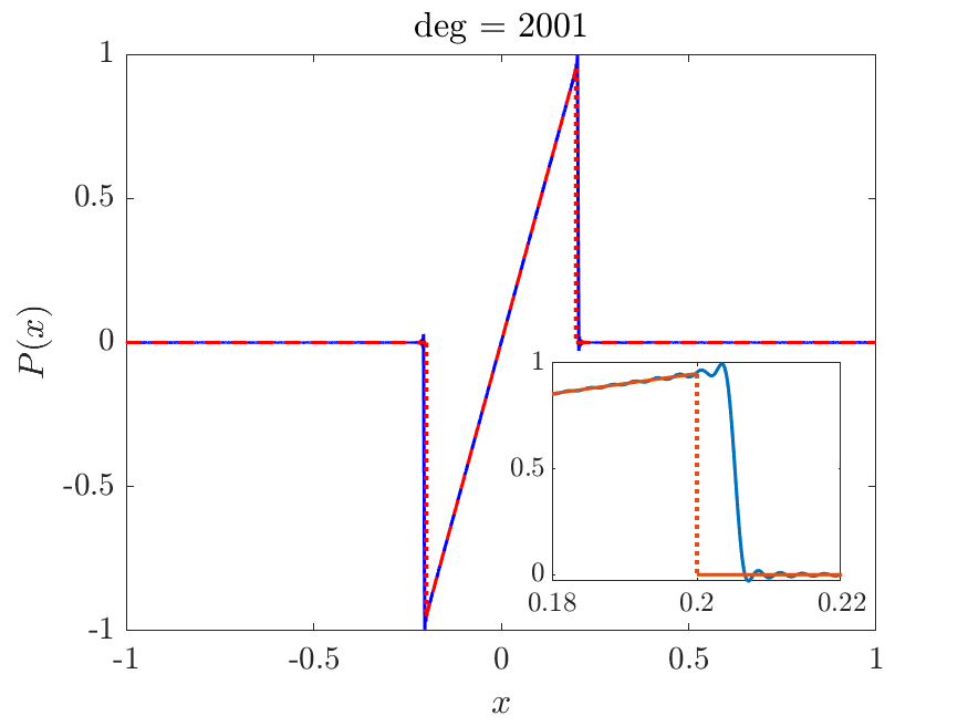
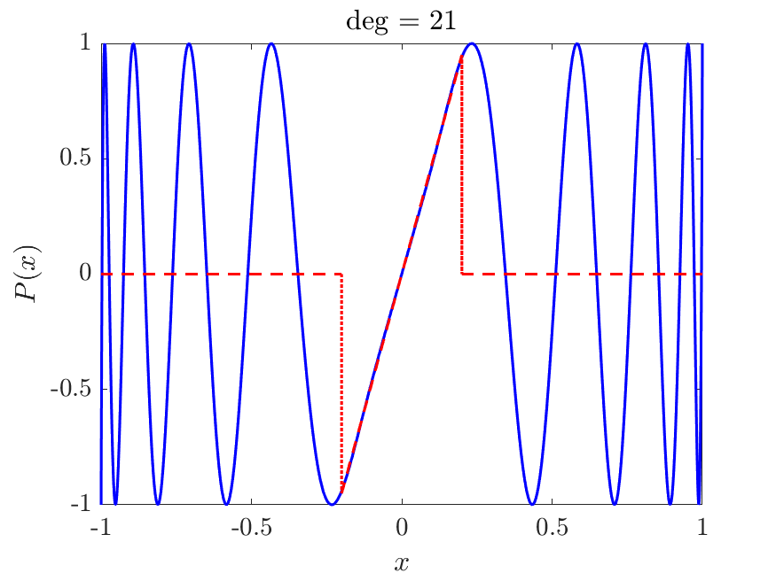
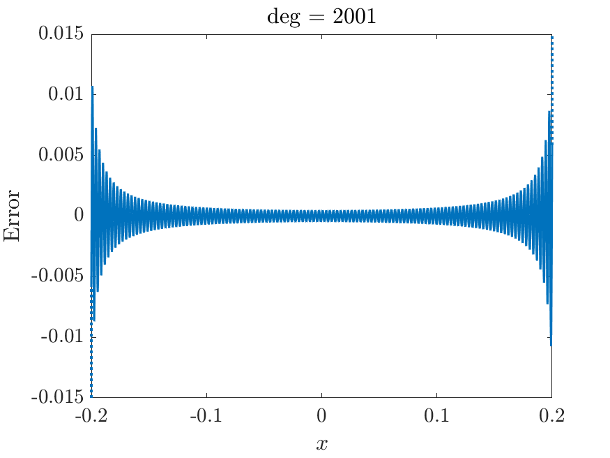
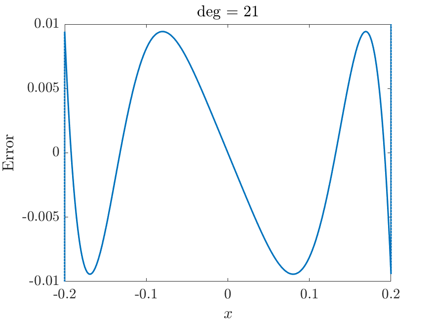
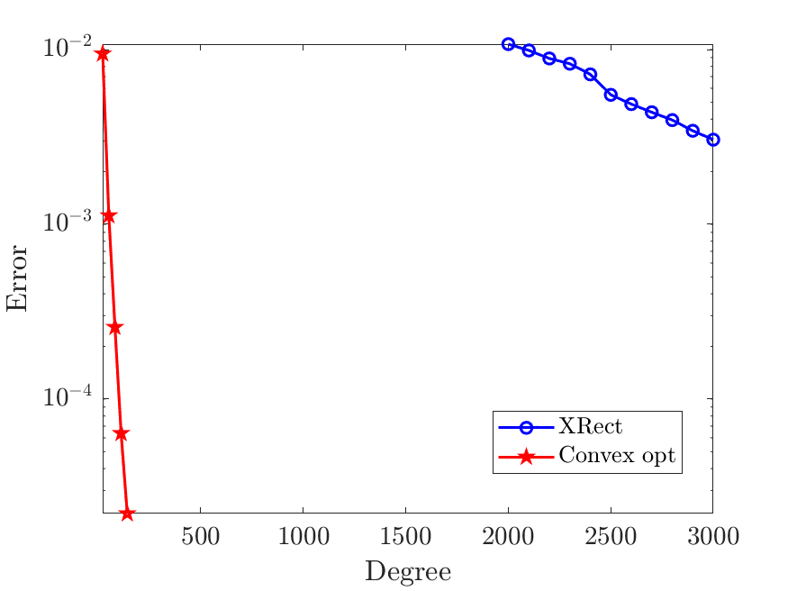
The desired odd polynomial is , which approximates , and agrees with the linear function on the interval . The polynomial should also satisfy the norm constraint: for all due to the requirement of QSVT (see [38, Corollary 5]). However, the function is discontinuous at , and therefore a polynomial approximation to exhibits the Gibbs phenomenon, which states that always overshoots around , even as the polynomial degree increases to infinity (see e.g., [39] and [62, Chapter 9]). An example of the Gibbs phenomenon is shown in the inset of Fig. 2 (a), where the polynomial approximation overshoots . As a result, instead of approximating , we can only find a polynomial that approximates the function to satisfy the norm constraint. It is worth mentioning that although the construction above leads to the desired asymptotic scaling in 2, the preconstant can be quite large, which leads to high polynomial degrees even for moderate values of the parameters . Fig. 2 (a) shows that for , the required polynomial degree is already as large as . Reducing to a smaller value would require a polynomial degree of around , which may be too large to be practically useful.
To address this issue, we notice that the uniform singular value amplification only requires us to find a polynomial that approximates on the desired interval . Outside this interval , the value of can be arbitrary, as long as the norm constraint is satisfied. In particular, does not need to approximate , which vanishes outside . This allows us to construct a convex optimization based procedure to numerically identify the near-optimal polynomial approximation for the uniform singular value amplification. The procedure is detailed in Appendix C. For the same parameter setting , the polynomial approximation is given in Fig. 2 (b) and the polynomial degree is merely . Fig. 2 (e) further shows that as fixing , both methods converge exponentially with respect to the increase of the polynomial degrees. However, the convergence rate of the convex optimization based method is significantly faster, which reduces the number of queries to by orders of magnitude.
2.4 Amplitude amplification using compression gadget
Since the main concern of running the algorithm in Fig. 1 is its success probability, it is natural to consider the usage of amplitude amplification [17] to reduce the number of repetitions needed to obtain a successful outcome. With the current procedure in Fig. 1, however, this results in a large space overhead. Directly applying (and hence ) sequentially involves intermediate measurements to determine whether each is applied successfully. We need to record the measurement outcome of each of the steps, and this means we need to duplicate the ancilla register times to implement amplitude amplification. To avoid this overhead, we need to replace the procedure with a fully coherent one, with measurement performed only at the end. This allows us to reduce the dependence from to .
Let us first formulate the problem in a more abstract way. We have unitaries , each of which is a -block encoding of a potentially non-unitary operation . The goal is to implement with amplitude amplification, and without duplicating the ancilla registers.
This goal can be achieved using the compression gadget in Fig. 3, following the idea in Ref. [57]. In fact we are using a simplified version of the compression gadget in Ref. [57], as the problem we are trying to solve is in some way easier. The main idea is to use a counter register to keep track of how many ’s have been applied successfully in a coherent way. This allows us to post-select on the counter register to ensure that all ’s have been applied successfully. This result is summarized in the following lemma. Its proof is given in Appendix D.
Lemma 3 (Compression gadget).
Suppose we are given unitaries , each of which is a -block encoding of . Then we can construct a -block encoding of , where
using one application of each .
\Qcircuit@R=1em @C=1em
Counter & \gateADD^L \gateADD^† \qw \gateADD^† \cds1⋯ \qw \gateADD^† \qw
Ancilla \multigate1V_1 \ctrlo-1 \multigate1V_2 \ctrlo-1 \qw \multigate1V_L \ctrlo-1 \qw
State \ghostV_1 \qw \ghostV_2 \qw \qw \ghostV_L \qw \qw
We can now use 3 to obtain the following result, taking into account the uniform singular value amplification procedure:
Theorem 4 (Coherent implementation of long-time integrator).
Suppose we are given through its -block encoding , for , and , then for any , we can construct an -block encoding of , where
| (17) |
and
| (18) |
using applications of each (controlled-) and its inverse.
Proof.
We denote by the matrix that is exactly encoded in each as in Eq. 14. Using Lemma 2, we first construct a -block encoding of each . Each uses times. Here we have used the fact that because of Eq. 13. We denote by the matrix that is exactly encoded in , i.e.,
Then
| (19) |
Next, we use Lemma 3 to combine ’s into a block encoding of . Directly applying Lemma 3 yields an -block encoding of , which we denote by , where
Noting the fact that
we can get the upper and lower bounds for through
To bound the error between and , we have
where for the second inequality we have used Eqs. 13 and 19, and for the last inequality we have used as well as . Therefore we can choose as in the statement of the corollary.
∎
With a coherent implementation of the long-time integrator given as a block encoding in 4, we can readily apply the standard amplitude amplification to boost the success probability and yield a quadratic speedup in terms of the query complexity.
3 High-order truncated Dyson series approach
In this section, we analyze the method described in Section 2, when the short time integrator is implemented using the high-order truncated Dyson series. In Section 3.1 we discuss how to implement the short time integrator developed in Ref. [57]. Then we use the tools developed in Sections 2.3 and 2.4 to link different segments of short time evolution into long time evolution in Section 3.2. We analyze the success probability in Section 3.3. Our time-marching based strategy can be combined with any input models such as the sparse matrix model [57, 7, 26, 48] and the linear combination of unitaries (LCU) model [57, 7]. We discuss in particular the implementation with a sparse matrix input model in Section 3.4.
3.1 Short time evolution
The truncated Dyson series method implements through
This infinite series can be truncated at order , and the error is upper bounded by . Therefore if we choose and so that , we can achieve high accuracy with only a few terms.
In order to be robust against error in the coefficient matrix, we need an additional step in the error analysis of the algorithm. If is accessed through an - as discussed in Section 2.2, then the above approach will yield a block encoding of a different time evolution operator , where is the time-dependent matrix encoded in exactly, as defined in Eq. 9. By 16, and assume that , then
With this additional step, using the same algorithm as in [57, Theorem 3], we can encode with the following costs:
Lemma 5 (Short-time evolution through truncated Dyson series).
Suppose , and is accessed through an - as defined in Definition 1 for some . , , where is the total variation of on the interval . Then we can construct an -block encoding of using queries to . Here and . We also use additional elementary gates.
In [57, Theorem 3], is chosen to satisfy
The discussion on the numerical quadrature error in Appendix F shows that we can further relax the regularity condition so that can be replaced by defined in Eq. 10.
3.2 Block encoding of the long time evolution operator
We choose ’s so that . Consequently the total number of segments are . For each segment , we construct a time-dependent matrix encoding of using the sparse matrix oracles in (27), and then implement the short time evolution operator . By 5, this procedure yields an -block encoding of , which we denote by . Since
the number of queries is . Each , and each satisfies
We need additional elementary gates and additional ancilla qubits as a working register. The working register starts in state and will be returned to at each time step, and can therefore be reused.
We introduce the shorthand notation
| (20) |
and use 4 to piece together the short time integrators into a block encoding approximating the long time evolution . This yields an -block encoding of , where
and
| (21) |
In this block encoding we use each times.
We now choose , and , . Also recall that . With this choice of parameters we have
| (22) |
and
| (23) |
Each is used times. Given the fact that each uses queries to times, and that there are of them, the total number of queries to are
| (24) |
We summarize the result of the construction of the block encoding for the long-time evolution using truncated Dyson series as follows.
Theorem 6 (Block encoding of long-time Dyson series evolution).
We assume , and is its total variation on . Suppose is accessed through an - as defined in 1. Let satisfy . We denote
Then we can construct an -block encoding of , where , and are given in Eqs. 22, 23 and 21, respectively. In this block encoding the number of times we need to use:
-
•
queries to as given by Eq. 24;
-
•
additional ancilla qubits that start in, and will be returned to ;
-
•
additional elementary gates.
3.3 Success probability and main result for Dyson series approach
We can now apply the block encoding to an initial state to get the final state . We assume that . Directly applying the block encoded time evolution operator will introduce an error, and we want to control the resulting error in the final normalized state. This can be done through the following lemma:
Lemma 7.
If , then
Proof.
Let . Then
| (25) | ||||
∎
We first use Theorem 6 to construct an -block encoding of . We denote this block encoding by . Let be the time evolution operator that is exactly encoded in . Then if we successfully prepare the state by applying the block encoding and measuring the ancilla qubits, the error will be
Therefore, by Lemma 7, in order to ensure that the error in the normalized state is upper bounded by , i.e.,
| (26) |
it suffices to choose .
Upon measuring the ancilla qubits, if all measurement outcomes are , then we have successfully prepared the state that approximates the exact solution . This happens with probability that is at least . Using the scaling of in Eq. 22, and the fact that , the success probability is , where
is the same as that defined in Eq. 4. Suppose that the initial state can be prepared using a unitary circuit , then we can boost the success probability to with rounds of amplitude amplification. With the above analysis, we can determine the cost of our algorithm, which we state in the following corollary.
Theorem 8 (Time-marching based solver using truncated Dyson series).
Let be the solution to the problem in Eq. 1. Suppose we have a unitary circuit that satisfies . For coefficient matrix , suppose . For each segment we have a time-dependent matrix encoding of denoted as that is an as defined in 1 for some , and for all . Then we can prepare, with probability at least , a quantum state that satisfies
using
queries to all , and applications of (controlled-) and its inverse. Here is defined in Eq. 4. In total we use qubits, and additional elementary gates. Success is flagged by the measurement result of a qubit.
3.4 Application to sparse matrix input model
In this section, we discuss the complexity of our time-marching strategy using the sparse matrix input model. The same input model has also been used in other QLSA-based differential equation solvers [8, 14, 26, 48] as well as time-dependent Hamiltonian simulation algorithms [7]. We assume that is a -sparse matrix with , and that the locations of non-zero elements are time-independent. The information of is given through the following oracles:
| (27) | ||||
Here is the row index of the th nonzero element in the th column, is the column index of the th nonzero element in the th row. We can use [37, Lemma 48] to construct in 1 using the sparse matrix oracles in Eq. 27. To construct a - we need a single query to both and , and two queries to . The precision parameter can be made arbitrarily small, but to keep the error below we need additional elementary gates and additional ancilla qubits are needed, where is the number of bits to encode the binary . These additional ancilla qubits can be reused.
Corollary 9 (Time-marching based solver using truncated Dyson series with sparse matrix input model).
Under the same assumptions in 8, together with the assumption that is a -sparse coefficient matrix given by unitaries , , and in Eq. 27we can prepare, with probability at least , a quantum state solving the problem in Eq. 1 that satisfies
using applications of (controlled-) , , and and their inverses, and applications of (controlled-) and its inverse. In total we use qubits, and additional elementary gates. Success is flagged by the measurement result of a qubit.
4 Optimality of the query complexity with respect to
In this section we show that the time-marching based solver using the high-order truncated Dyson series achieves the nearly optimal query complexity with respect to the amplification ratio . The optimality is guaranteed by the following lower bound result. Although we state this lower bound result in terms of a time-independent ODE, it automatically provides a lower bound for the harder problem of solving a time-dependent ODE in Eq. 1. The block encoding of the coefficient matrix also automatically provides a time-dependent matrix encoding needed in Theorem 8.
Theorem 10.
For any given , there exists a matrix that can be accessed through its -block encoding , a target time , and an initial state with such that the following statement holds: Let be the solution of the ODE with , i.e., . Then for any , there is no quantum algorithm that can prepare a quantum state (allowed to be a mixed state) with , which uses queries to . Here denotes the trace distance between two quantum states and
| (28) |
Proof.
We assume towards contradiction that such an algorithm exists. Now we apply this hypothetical algorithm to solve the unstructured search problem, in which we are asked to find a marked binary string of length . We denote . The target is marked by the following oracle :
Here is any binary string of length that is different from .
We let , then is an -block encoding of . Solving the ODE up to time yields us a (unnormalized) state
Note that in this quantum state, the amplitude corresponding to the marked element is amplified, while the amplitudes corresponding to all other elements are suppressed. Consequently, the probability getting when measuring the state in the computational basis increases with time. At time , this probability is
If we set , then the above probability will be . Suppose we can prepare a state with , then
As a result, once we prepare a copy of , we can measure in the computational basis, and with probability at least we will get the marked element . We can use one application of to check whether the measurement output is . Therefore in order to find with probability , we only need copies of .
Let us then look at the cost of preparing . With the hypothetical algorithm for solving the ODE, we can prepare using queries to . Here as chosen above, and in this scenario
Therefore, we need queries to prepare a single copy of . Since only copies are needed, we would then be able to solve the unstructured search problem using only queries to the oracle . This contradicts the lower bound for the unstructured search problem [6, Corollary 3.5]. ∎
It is worth noting that the lower bound result in 10 does not imply that the dependence on cannot be improved for specific instances of . For example, consider the following non-diagonalizable matrix
| (29) |
Direct calculation shows that , and therefore grows linearly in . However,
| (30) |
grows exponentially in , and so is in Eq. 28. Applying the result of [48], we know that the cost of the optimal solver should grow as for any . Therefore our time-marching based algorithm is suboptimal in this case. Note that if is a normal matrix, the quantity in Eq. 30 is equal to , and this issue does not arise.
5 Simplified implementation and first-order truncated Magnus series
The time-marching strategy can be paired with any reasonable short-time integrators. The implementation of the high-order truncated Dyson series algorithms requires complicated quantum control logic for handling time-ordering operators. In this section, we investigate the performance of time-marching based algorithms with low-order integrators that can be implemented without the explicit treatment of time-ordering operators. The simplest example is a first-order truncated Dyson series algorithm:
| (31) |
We can approximate the integral using numerical quadrature as in the implementation of the high-order truncated Dyson series.
A closely related first-order integrator takes the form
| (32) |
i.e., we perform the matrix exponentiation of the time-independent matrix directly without further Taylor expansion. This is the first-order truncated Magnus series for approximating the time-ordered integration. In the context of Hamiltonian simulation, this strategy gives rise to the quantum highly oscillatory protocol (qHOP) [4], which exhibits commutator scaling in high-precision limit, can be insensitive to the norm and the variation of , and can lead to second-order convergence (i.e., superconvergence) for certain . The rest of the section analyzes the scheme (32) for solving the ODE (1). We verify that this scheme also exhibits the desired commutator scaling. An extreme example where this is useful is when commutes with itself at any time, then (32) becomes exact, which leads to improved accuracy and poly-logarithmic dependence in the query complexity on the precision. For general non-commuting case, we can use higher order truncation of the Magnus series to improve the accuracy dependence while keeping the commutator scaling. However, the implementation of the quantum circuit can be more complicated.
5.1 Short-time evolution description
For each short time evolution, the time-ordered evolution operator is approximated by truncating its first-order Magnus expansion (32), which is equivalent to directly ignoring the time-ordering operator. The integral can be further approximated using standard Riemann sum with quadrature points () as
| (33) |
The short-time first-order Magnus evolution operator, denoted as is thus given as
| (34) |
The implementation of the short-time first-order Magnus evolution operator in two steps. The first step is to construct the block encoding of (33) via applying on the qubits where HAD represents the single qubit Hadamard gate, applying MAT and then uncomputing, namely
| (35) |
The quantum circuit of implementing Eq. 35 is described in Fig. 4.
The second step is to implement the time-independent matrix exponential via a contour integral formulation combined with QSVT, as detailed in Appendix G. The observation is that for general that are not normal, the singular value transformation no longer agrees with the eigenvalue transformation. Nevertheless, the matrix exponential can be applied by exploring the contour integral formulation proposed in [61]. The idea is to express as a contour integral:
| (36) |
where is a contour in the complex plane that contains all the eigenvalues of in its interior. We then discretize the integral using numerical quadrature. This procedure turns the matrix exponential into a linear combination of , which can be efficiently calculated as matrix inversion problems that does not require the matrix being normal. Here ’s are some constants determined by the numerical quadrature, which is detailed in Section 5.3. We also remark that there are certain cases of where admits a simpler implementation using QSVT via polynomial approximations of the exponential function [37, Corollary 64]. Ref. [59] also developed a method to apply a more general class of matrix functions using the contour integral, but they did not consider how to construct a block encoding, instead focusing on preparing the output state.
\Qcircuit@R=1em @C=1em
Ancilla & \qw \multigate2MAT_j \qw \qw
Control \gate⊗_qHAD \ghostMAT_j \gate⊗_qHAD \qw
State \qw \ghostMAT_j \qw \qw
5.2 Time discretization error
We now analyze the time-discretization error for the short-time evolution.
Lemma 11 (Time discretization errors of the first-order Magnus integrator).
Let denote the exact evolution operator on the time interval , and denote the first-order Magnus operator defined in Eq. 34. Then we have
| (37) |
Proof.
The errors come from two parts: one from dropping the time-ordering operator, while the other from the numerical quadrature. To estimate the error, we introduce the notations of the exact evolution from time to as
so that , and the matrix after dropping the time-ordering operator as
| (38) |
We first study the approximation error between the two. For any , by differentiating with respect to , we have
| (39) |
The difference between and satisfies the differential equation
| (40) |
and by the variation of parameter formula [18], we have
| (41) |
where
and
Applying the fundamental theorem of calculus in terms of yields that
Note that the exponential factor here is bounded quite loose, and in fact one can get a sharper bound by using the logarithmic norm. But here for our purposes, it is sufficient to estimate at the level of . Another useful fact is
| (42) |
which can be shown by applying the Gronwall’s inequality in terms of to
where is the fundamental matrix. Thus, the approximation error of the first part can be summarized as
| (43) |
We now estimate the error induced by the numerical quadrature using the total variation. Following the result in Appendix F, we have
| (44) |
where we recall that is the total variation of on the interval . Furthermore, the variation of parameter formula gives that for square matrices and ,
which implies that
| (45) |
Therefore,
| (46) |
5.3 Algorithm for implementing
In order to discuss the complexity of implementing the short-time first-order Magnus evolution operator, we first briefly discuss in this section how to implement a matrix exponential of a general time-independent matrix, namely to implement , when is given through its -block encoding. The details are laid out in Appendix G.
The main idea is to use the contour integral representation of a matrix function
| (47) |
where is a unit circle with radius : . This contour integral can be discretized as
| (48) |
for . The error that comes from this discretization can be analyzed using Lemma 18, which is modified from [63, Theorem 18.1] and [59, Proposition 5]. We choose , , and by Lemma 18 we have
| (49) |
Our goal is to construct a block encoding of using (48). We will proceed as follows: we first construct a block encoding of
| (50) |
where . Inverting using QSVT gives us
| (51) |
Now suppose we can prepare quantum states , that satisfy
then we obtain the desired block encoding
| (52) |
Here for a complex number , can be any such that .
To construct this block encoding we need additional ancilla qubits. The entire circuit acts on five different registers, as shown in Figure 6. The first register contains one qubit and is used for matrix inversion through QSVT. The second register contains qubits to encode the coefficients in the amplitude. The third register contains one qubit and is used in the block encoding of each . The fourth register contains qubits, and this is the ancilla register used in the block encoding . The fifth register contains qubits and is the qubits that acts on. We will use to denote the identity operator acting on qubits.
The cost of this implementation can be summarized in the following lemma, whose proof is laid out in Appendix G.
Lemma 12 (Matrix exponentiation).
Given a -block encoding of , we can construct a -block encoding of , with applications of (controlled-) and its inverse, and additional elementary gates. Here
where .
5.4 Short-time complexity of the first-order integrator
The cost of constructing a block encoding of the short-time first-order Magnus evolution operator is given by the following lemma.
Lemma 13 (Short-time evolution through the first-order Magnus integrator).
Suppose , and is accessed through an - as defined in Definition 1 for some . Let
and . Choose
where is the total variation of on the interval . Then we can construct an -block encoding of , with
This requires
-
•
queries to ,
-
•
additional elementary gates.
Proof.
is a time-dependent matrix encoding of with precision , and is hence a time-dependent matrix encoding of with precision by 1.
We first consider the cost of constructing the block encoding of
Let . As depicted in (35), one can construct a block encoding of , using query to and additional one-qubit gates.
We then use QSVT and contour integral formulation 12 to implement . Then we obtain the following
block encoding of , where
This uses queries to the block encoding of and hence queries to . The additional elementary gates needed for this procedure is
We now control the error between and . Denote
We first consider the error between and . Notice that
By (45), we have
Choose
so that
Thanks to 11, the error
By our choice of and we have that the right-hand-side is bounded by , as
Therefore, we get a
block encoding of .
∎
5.5 Block encoding of the long-time evolution operator
For simplicity, we choose a uniform temporal mesh. Let so that where is the number of time steps. We perform the short-time first-order Magnus evolution on each interval and multiply all the evolution together.
By 13, each short-time first-order Magnus evolution on yields a -block encoding (denoted ) of , where
and is an upper bound of
The construction uses queries to and additional elementary gates with .
Applying 4, we get a -block encoding of with
Here
and
| (53) |
where is an upper bound of
In this block encoding we use applications of each .
Denote the upper bound of the time average -scaling as . Thanks to our choice of ’s, each can be upper bounded by . Choose
where
| (54) |
With this choice of parameters we have
| (55) |
and
| (56) |
Each is used
times. Given the fact that each uses queries to times, and that there are of them, the total number of queries to all are
| (57) | ||||
| (58) |
Note that when , this first-order truncated series implementation in fact has the same complexity scaling as the high-order truncated Dyson series. We remark that it is also possible to get the scaling , by varying time step sizes in the propagation according to the average performance of the Hamiltonian as in [7, 4]: Let where is the number of time steps and are chosen such that
| (59) |
which we shall not discuss more details here.
5.6 Success probability and main result paired with first-order integrator
The success probability of the first-order Magnus method follows a similar argument as the Dyson series approach as detailed in Section 3.3. It suffices to choose and the success probability is at least . Suppose that the initial state can be prepared using a unitary circuit , then we can boost the success probability to with rounds of amplitude amplification. We can conclude the result when pairing the time-marching strategy with the first-order Magnus-type integrator for long time evolution as follows.
Theorem 14 (The time-marching differential equation solver paired with the first-order Magnus integrator).
Let be the solution to the ODE . Suppose we have a unitary circuit that satisfies . For a coefficient matrix , suppose , and for each segment we have a time-dependent matrix encoding of denoted as that is an as defined in 1 for some . Let be the total variation of on as defined in (10). We can prepare, with probability at least , a quantum state that satisfies
using
total number of queries to all , and applications of (controlled-) and its inverse. In particular, in the high-precision limit given a non-zero , the total number of queries to all can be simplified as
In total we use qubits. Here is defined as (4), and is defined in Eq. (54). Success is flagged by the measurement result of a qubit.
6 Discussion
We revisit the time-marching strategy for solving the ODE (1), and demonstrate that it can be a useful alternative to QLSA based quantum differential equation solvers. On a technical level, our time-marching based algorithm achieves the following tasks for the first time: (1) It has provable performance guarantees for non-diagonalizable, and time-dependent dynamics. (2) It retains high-order accuracy for non-smooth . (3) It can use few queries to the initial state. For inhomogeneous linear differential equations , we may use the variation of constants to express the solution as
| (60) |
After discretization of the integration with respect to , this is reduced to a series of homogeneous linear differential equations that can be implemented by the time-marching method. The analysis for the inhomogeneous case can thus be similar using the tools developed in this paper.
At a high level, time-marching based methods and QLSA based methods simply amount to two different ways of rearranging the same identities of the form . However, there are many differences between these two classes of algorithms, and we do not know whether the gaps can be closed with further improvements, or are intrinsic to each type of the method. For instance, it is possible to refine the complexity analysis of QLSA based algorithms so that the cost does not directly depend on the condition number , or to improve the algorithm so that it achieves high-order accuracy for non-smooth [16]. However, it is unclear whether the number of queries to the initial state of any QLSA based algorithm can be independent of . For time-marching based algorithms, though the dependence on the precision is near-optimal and scales as , the dependence of the query complexity to the input matrix is . We do not know whether the scaling in the query complexity to the matrix can be improved, or whether the dependence on can be weakened to . It is also possible that another class of algorithms is needed to provide a unifying perspective to the questions above, and to achieve near-optimal complexity with respect to all parameters.
Acknowledgments
This work was partially supported by the NSF Quantum Leap Challenge Institute (QLCI) program under Grant No. OMA-2016245 and NSF DMS-2208416 (D.F.), by the U.S. Department of Energy under the Quantum Systems Accelerator program under Grant No. DE-AC02-05CH11231 (Y.T.), and by a Google Quantum Research Award (L.L.). L.L. is a Simons Investigator. We thank Dong An, Dominic Berry, Andrew Childs and Jin-Peng Liu for discussions.
References
- [1] A. Ambainis. Variable time amplitude amplification and quantum algorithms for linear algebra problems. In Leibniz Int. Proc. Informatics, LIPIcs, volume 14, pages 636–647, 2012. doi:10.4230/LIPIcs.STACS.2012.636.
- [2] D. An, D. Fang, S. Jordan, J.-P. Liu, G. H. Low, and J. Wang. Efficient quantum algorithm for nonlinear reaction-diffusion equations and energy estimation, 2022. URL: http://arxiv.org/abs/2205.01141, arXiv:2205.01141, doi:10.48550/ARXIV.2205.01141.
- [3] D. An, D. Fang, and L. Lin. Time-dependent unbounded Hamiltonian simulation with vector norm scaling. Quantum, 5:1–49, may 2021. URL: https://doi.org/10.22331/q-2021-05-26-459, arXiv:2012.13105, doi:10.22331/Q-2021-05-26-459.
- [4] D. An, D. Fang, and L. Lin. Time-dependent Hamiltonian Simulation of Highly Oscillatory Dynamics and Superconvergence for Schrödinger Equation. Quantum, 6:690, apr 2022. doi:10.22331/q-2022-04-15-690.
- [5] D. An and L. Lin. Quantum Linear System Solver Based on Time-optimal Adiabatic Quantum Computing and Quantum Approximate Optimization Algorithm. ACM Trans. Quantum Comput., 3(2):1–28, 2022. arXiv:1909.05500, doi:10.1145/3498331.
- [6] C. H. Bennett, E. Bernstein, G. Brassard, and U. Vazirani. Strengths and weaknesses of quantum computing. SIAM journal on Computing, 26(5):1510–1523, 1997. doi:10.1137/S0097539796300933.
- [7] D. Berry, A. M. Childs, Y. Su, X. Wang, and N. Wiebe. Time-dependent Hamiltonian simulation with -norm scaling. Quantum, 4:254, 2020. doi:10.22331/q-2020-04-20-254.
- [8] D. W. Berry. High-order quantum algorithm for solving linear differential equations. Journal of Physics A: Mathematical and Theoretical, 47(10):105301, feb 2014. doi:10.1088/1751-8113/47/10/105301.
- [9] D. W. Berry, G. Ahokas, R. Cleve, and B. C. Sanders. Efficient quantum algorithms for simulating sparse hamiltonians. Commun. Math. Phys., 270(2):359–371, 2007. arXiv:0508139, doi:10.1007/s00220-006-0150-x.
- [10] D. W. Berry and A. M. Childs. Black-box hamiltonian simulation and unitary implementation. Quantum Inf. Comput., 12(1-2):29–62, 2012. arXiv:0910.4157, doi:10.26421/QIC12.1-2.
- [11] D. W. Berry, A. M. Childs, R. Cleve, R. Kothari, and R. D. Somma. Exponential improvement in precision for simulating sparse Hamiltonians. In Proc. Annu. ACM Symp. Theory Comput., pages 283–292, 2014. arXiv:1312.1414, doi:10.1145/2591796.2591854.
- [12] D. W. Berry, A. M. Childs, R. Cleve, R. Kothari, and R. D. Somma. Simulating hamiltonian dynamics with a truncated taylor series. Phys. Rev. Lett., 114(9):90502, 2015. arXiv:1412.4687, doi:10.1103/PhysRevLett.114.090502.
- [13] D. W. Berry, A. M. Childs, and R. Kothari. Hamiltonian Simulation with Nearly Optimal Dependence on all Parameters. Proc. - Annu. IEEE Symp. Found. Comput. Sci. FOCS, 2015-December:792–809, 2015. arXiv:1501.01715, doi:10.1109/FOCS.2015.54.
- [14] D. W. Berry, A. M. Childs, A. Ostrander, and G. Wang. Quantum algorithm for linear differential equations with exponentially improved dependence on precision. Communications in Mathematical Physics, 356(3):1057–1081, 2017. doi:10.1007/s00220-017-3002-y.
- [15] D. W. Berry, R. Cleve, and S. Gharibian. Gate-efficient discrete simulations of continuous-time quantum query algorithms. Quantum Inf. Comput., 14(1-2):1–30, 2014. doi:10.26421/qic14.1-2-1.
- [16] D. W. Berry and P. C. S. Costa. Quantum algorithm for time-dependent differential equations using dyson series, 2022. URL: https://arxiv.org/abs/2212.03544, doi:10.48550/ARXIV.2212.03544.
- [17] G. Brassard, P. Høyer, M. Mosca, and A. Tapp. Quantum amplitude amplification and estimation. Contemp. Math., 305:53–74, 2002. arXiv:0005055, doi:10.1090/conm/305/05215.
- [18] F. Brauer and J. A. Nohel. The Qualitative Theory of Ordinary Differential Equations: An Introduction. Dover Books on Mathematics. Dover Publications, 2012. URL: https://books.google.com/books?id=9qPsbRl7hBkC.
- [19] R. L. Burden, J. D. Faires, and A. C. Reynolds. Numerical analysis. Brooks Cole, 2000.
- [20] E. Campbell. Random Compiler for Fast Hamiltonian Simulation. Phys. Rev. Lett., 123(7):70503, 2019. arXiv:1811.08017, doi:10.1103/PhysRevLett.123.070503.
- [21] S. Chakraborty, A. Gilyén, and S. Jeffery. The power of block-encoded matrix powers: Improved regression techniques via faster Hamiltonian simulation. Leibniz Int. Proc. Informatics, LIPIcs, 132, 2019. arXiv:1804.01973, doi:10.4230/LIPIcs.ICALP.2019.33.
- [22] R. Chao, D. Ding, A. Gilyen, C. Huang, and M. Szegedy. Finding Angles for Quantum Signal Processing with Machine Precision. 2020. URL: http://arxiv.org/abs/2003.02831, arXiv:2003.02831, doi:10.48550/arXiv.2003.02831.
- [23] C.-F. Chen, Hsin-Yuan, Huang, R. Kueng, and J. a. Tropp. Concentration for random product formulas. arXiv:2008.11751, page 25, 2020. URL: http://arxiv.org/abs/2008.11751, arXiv:2008.11751, doi:10.1103/PRXQuantum.2.040305.
- [24] Y. H. Chen, A. Kalev, and I. Hen. Quantum Algorithm for Time-Dependent Hamiltonian Simulation by Permutation Expansion. PRX Quantum, 2(3):30342, sep 2021. URL: https://link.aps.org/doi/10.1103/PRXQuantum.2.030342, arXiv:2103.15334, doi:10.1103/PRXQuantum.2.030342.
- [25] A. M. Childs, R. Kothari, and R. D. Somma. Quantum algorithm for systems of linear equations with exponentially improved dependence on precision. SIAM J. Comput., 46(6):1920–1950, 2017. arXiv:1511.02306, doi:10.1137/16M1087072.
- [26] A. M. Childs and J. P. Liu. Quantum Spectral Methods for Differential Equations. Commun. Math. Phys., 375(2):1427–1457, 2020. arXiv:1901.00961, doi:10.1007/s00220-020-03699-z.
- [27] A. M. Childs, D. Maslov, Y. Nam, N. J. Ross, and Y. Su. Toward the first quantum simulation with quantum speedup. Proc. Natl. Acad. Sci. U. S. A., 115(38):9456–9461, 2018. arXiv:1711.10980, doi:10.1073/pnas.1801723115.
- [28] A. M. Childs, A. Ostrander, and Y. Su. Faster quantum simulation by randomization. Quantum, 3:182, 2019. arXiv:1805.08385, doi:10.22331/q-2019-09-02-182.
- [29] A. M. Childs and Y. Su. Nearly Optimal Lattice Simulation by Product Formulas. Phys. Rev. Lett., 123(5):50503, 2019. arXiv:1901.00564, doi:10.1103/PhysRevLett.123.050503.
- [30] A. M. Childs, Y. Su, M. C. Tran, N. Wiebe, and S. Zhu. Theory of Trotter Error with Commutator Scaling. Phys. Rev. X, 11(1):11020, 2021. doi:10.1103/PhysRevX.11.011020.
- [31] A. M. Childs and N. Wiebe. Hamiltonian simulation using linear combinations of unitary operations. Quantum Inf. Comput., 12(11-12):901–924, nov 2012. URL: http://dx.doi.org/10.26421/QIC12.11-12, arXiv:1202.5822, doi:10.26421/qic12.11-12-1.
- [32] P. C. Costa, D. An, Y. R. Sanders, Y. Su, R. Babbush, and D. W. Berry. Optimal scaling quantum linear-systems solver via discrete adiabatic theorem. PRX Quantum, 3:040303, Oct 2022. URL: https://link.aps.org/doi/10.1103/PRXQuantum.3.040303, doi:10.1103/PRXQuantum.3.040303.
- [33] P. C. S. Costa, S. Jordan, and A. Ostrander. Quantum algorithm for simulating the wave equation. Physical Review A, 99(1):012323, 2019. arXiv:1711.05394. doi:10.1103/PhysRevA.99.012323.
- [34] I. Y. Dodin and E. A. Startsev. On applications of quantum computing to plasma simulations. Physics of Plasmas, 28(9):092101, 2021. doi:10.1063/5.0056974.
- [35] Y. Dong, X. Meng, K. B. Whaley, and L. Lin. Efficient phase-factor evaluation in quantum signal processing. Phys. Rev. A, 103(4), 2021. arXiv:2002.11649, doi:10.1103/PhysRevA.103.042419.
- [36] A. Engel, G. Smith, and S. E. Parker. Linear embedding of nonlinear dynamical systems and prospects for efficient quantum algorithms. Physics of Plasmas, 28(6):062305, 2021. arXiv:2012.06681. doi:10.1063/5.0040313.
- [37] A. Gilyén, Y. Su, G. H. Low, and N. Wiebe. Quantum singular value transformation and beyond: exponential improvements for quantum matrix arithmetics. arXiv preprint arXiv:1806.01838, 2018. doi:10.48550/arXiv.1806.01838.
- [38] A. Gilyén, Y. Su, G. H. Low, and N. Wiebe. Quantum singular value transformation and beyond: exponential improvements for quantum matrix arithmetics. In Proc. 51st Annu. ACM SIGACT Symp. Theory Comput., pages 193–204, 2019. doi:10.1145/3313276.3316366.
- [39] D. Gottlieb and C.-W. Shu. On the Gibbs phenomenon and its resolution. SIAM Rev., 39(4):644–668, 1997. doi:10.1137/S0036144596301390.
- [40] M. Grant and S. Boyd. CVX: Matlab software for disciplined convex programming, version 2.1. http://cvxr.com/cvx, Mar. 2014.
- [41] J. Haah. Product decomposition of periodic functions in quantum signal processing. Quantum, 3:190, 2019. arXiv:1806.10236, doi:10.22331/q-2019-10-07-190.
- [42] E. Hairer, C. Lubich, and G. Wanner. Geometric Numerical Integration: Structure-Preserving Algorithms for Ordinary Differential Equations (Springer Series in Computational Mathematics), volume 31. Springer, 2006.
- [43] E. Hairer, S. P. Nørsett, and G. Wanner. Solving ordinary differential equations I. nonstiff problems, volume 29. Springer, 1987. doi:10.1016/0378-4754(87)90083-8.
- [44] A. W. Harrow, A. Hassidim, and S. Lloyd. Quantum algorithm for linear systems of equations. Phys. Rev. Lett., 103(15):150502, 2009. doi:10.1103/PhysRevLett.103.150502.
- [45] S. Jin and N. Liu. Quantum algorithms for computing observables of nonlinear partial differential equations, 2022. arXiv:2202.07834. doi:10.48550/arXiv.2202.07834.
- [46] I. Joseph. Koopman-von Neumann approach to quantum simulation of nonlinear classical dynamics. Physical Review Research, 2(4):043102, 2020. arXiv:2003.09980. doi:10.1103/PhysRevResearch.2.043102.
- [47] M. Kieferová, A. Scherer, and D. W. Berry. Simulating the dynamics of time-dependent Hamiltonians with a truncated Dyson series. Phys. Rev. A, 99(4), apr 2019. URL: http://dx.doi.org/10.1103/PhysRevA.99.042314, arXiv:1805.00582, doi:10.1103/PhysRevA.99.042314.
- [48] H. Krovi. Improved quantum algorithms for linear and nonlinear differential equations, 2022. URL: http://arxiv.org/abs/2202.01054, arXiv:2202.01054, doi:10.48550/ARXIV.2202.01054.
- [49] L. Lin and Y. Tong. Optimal polynomial based quantum eigenstate filtering with application to solving quantum linear systems. Quantum, 4:361, 2020. doi:10.22331/q-2020-11-11-361.
- [50] N. Linden, A. Montanaro, and C. Shao. Quantum vs. classical algorithms for solving the heat equation. Comm. Math. Phys., 395(2):601–641, 2022. doi:10.1007/s00220-022-04442-6.
- [51] J.-P. Liu, H. Ø. Kolden, H. K. Krovi, N. F. Loureiro, K. Trivisa, and A. M. Childs. Efficient quantum algorithm for dissipative nonlinear differential equations. Proceedings of the National Academy of Sciences, 118(35), 2021. arXiv:2011.03185. doi:10.1073/pnas.2026805118.
- [52] S. Lloyd, G. De Palma, C. Gokler, B. Kiani, Z.-W. Liu, M. Marvian, F. Tennie, and T. Palmer. Quantum algorithm for nonlinear differential equations, 2020. arXiv:2011.06571. doi:10.48550/arXiv.2011.06571.
- [53] G. H. Low. Hamiltonian simulation with nearly optimal dependence on spectral norm. In Proc. Annu. ACM Symp. Theory Comput., pages 491–502, 2019. arXiv:1807.03967, doi:10.1145/3313276.3316386.
- [54] G. H. Low and I. L. Chuang. Hamiltonian simulation by uniform spectral amplification. arXiv:1707.05391, 2017. doi:10.48550/arXiv.1707.05391.
- [55] G. H. Low and I. L. Chuang. Optimal Hamiltonian Simulation by Quantum Signal Processing. Phys. Rev. Lett., 118(1):10501, 2017. arXiv:1606.02685, doi:10.1103/PhysRevLett.118.010501.
- [56] G. H. Low and I. L. Chuang. Hamiltonian simulation by qubitization. Quantum, 3:163, 2019. arXiv:1610.06546, doi:10.22331/q-2019-07-12-163.
- [57] G. H. Low and N. Wiebe. Hamiltonian Simulation in the Interaction Picture. arXiv:1805.00675, 2018. URL: http://arxiv.org/abs/1805.00675, arXiv:1805.00675, doi:10.48550/arXiv.1805.00675.
- [58] Y. Subaşl, R. D. Somma, and D. Orsucci. Quantum algorithms for systems of linear equations inspired by adiabatic quantum computing. Phys. Rev. Lett., 122(6):60504, 2019. arXiv:1805.10549, doi:10.1103/PhysRevLett.122.060504.
- [59] S. Takahira, A. Ohashi, T. Sogabe, and T. S. Usuda. Quantum algorithm for matrix functions by cauchy’s integral formula. Quantum Inf. Comput., 20(1-2):14–36, 2020. arXiv:2106.08075, doi:10.26421/qic20.1-2-2.
- [60] Y. Tong, V. V. Albert, J. R. McClean, J. Preskill, and Y. Su. Provably accurate simulation of gauge theories and bosonic systems, 2021. URL: https://arxiv.org/abs/2110.06942, doi:10.48550/ARXIV.2110.06942.
- [61] Y. Tong, D. An, N. Wiebe, and L. Lin. Fast inversion, preconditioned quantum linear system solvers, fast Green’s-function computation, and fast evaluation of matrix functions. Phys. Rev. A, 104(3), 2021. doi:10.1103/PhysRevA.104.032422.
- [62] L. N. Trefethen. Approximation Theory and Approximation Practice, Extended Edition, volume 164. SIAM, 2019. doi:10.1137/1.9781611975949.
- [63] L. N. Trefethen and J. A. Weideman. The exponentially convergent trapezoidal rule. SIAM Rev., 56(3):385–458, 2014. doi:10.1137/130932132.
- [64] C. Tronci and I. Joseph. Koopman wavefunctions and Clebsch variables in Vlasov-Maxwell kinetic theory, 2021. doi:10.1017/S0022377821000805.
- [65] J. Wang, Y. Dong, and L. Lin. On the energy landscape of symmetric quantum signal processing. Quantum, 6:850, Nov. 2022. doi:10.22331/q-2022-11-03-850.
- [66] D. Wecker, M. B. Hastings, N. Wiebe, B. K. Clark, C. Nayak, and M. Troyer. Solving strongly correlated electron models on a quantum computer. Phys. Rev. A - At. Mol. Opt. Phys., 92(6):62318, 2015. arXiv:1506.05135, doi:10.1103/PhysRevA.92.062318.
- [67] N. Wiebe, D. Berry, P. Høyer, and B. C. Sanders. Higher order decompositions of ordered operator exponentials. J. Phys. A Math. Theor., 43(6), 2010. arXiv:0812.0562, doi:10.1088/1751-8113/43/6/065203.
- [68] L. Ying. Stable factorization for phase factors of quantum signal processing. Quantum, 6:842, Oct. 2022. doi:10.22331/q-2022-10-20-842.
- [69] B. Şahinoğlu and R. D. Somma. Hamiltonian simulation in the low-energy subspace. npj Quantum Inf., 7(1), 2021. arXiv:2006.02660, doi:10.1038/s41534-021-00451-w.
Appendix A Notations
Throughout the paper, denotes the spectral norm of a matrix , denotes 2-norm of a vector , and denotes the trace distance between two quantum states defined as
We use the following asymptotic notations besides the usual notation: we write if ; if and ; if . For two quantum states and , we sometimes write to denote . The notations regarding each short time evolution can be summarized as follows. Note that the same can be viewed as a block encoding of and , and the difference is only in the error of the block encoding.
| Notation | Meaning | Corresponding block encoding |
| the exact time evolution operator | is an -block encoding of | |
| an approximation of the exact evolution | is an -block encoding of | |
| after uniform singular value amplification | is a -block encoding of |
Appendix B Block encoding and quantum singular value transformation
We call a matrix an -qubit matrix or an -qubit operator. In this work we extensively use the technique of block encoding [56, 21, 38], which is a way of embedding an arbitrary matrix as a sub-matrix of a larger unitary matrix. Using a unitary matrix to encode as a sub-matrix means that there exist a subnormalization factor such that
| (61) |
where denotes arbitrary matrix blocks of proper sizes. In general, the matrix that we block encode may only approximate, but is not exactly equal to, . We use the following notation to describe such encodings.
Definition 15 (Block encoding, [38]).
An -qubit unitary operator is called an -block encoding of an -qubit operator , if
Here is the number of ancilla qubits for block encoding, and is called the subnormalization factor. With the -block encoding , we can perform a quantum singular value transformation (QSVT) of on a quantum computer using the technique developed in [38]. More precisely, suppose has a singular value decomposition , then for any odd polynomial with degree such that for , we can construct a block encoding of , and this block encoding uses times. This is the main tool for implementing the uniform singular value amplification in Lemma 2. QSVT requires finding a sequence of phase factors corresponding to the polynomial we want to implement. There are classical algorithms capable of doing this [41] in polynomial time, and later works developed more efficient methods for high-degree polynomials with high precision requirements [22, 35, 65, 68].
Appendix C Convex optimization based method for uniform singular value amplification
In order to approximate an odd target function using an odd polynomial of degree , we can express the target polynomial as the linear combination of Chebyshev polynomials with some unknown coefficients :
| (62) |
To formulate this as a discrete optimization problem, we first discretize using grid points (e.g., roots of Chebyshev polynomials ). We define the coefficient matrix, . Then the coefficients for approximating the polynomial used for uniform singular value amplification can be found by solving the following optimization problem
| (63) |
This is a convex optimization problem and can be solved using software packages such as CVX [40]. The norm constraint is relaxed to to take into account that the constraint can only be imposed on the sampled points, and the values of may slightly overshoot on . The effect of this relaxation can be negligible when we choose to be sufficiently close to (for instance, can be ). Since Eq. 63 approximately solves a min-max problem, it achieves the near-optimal solution (in the sense of the norm) by definition both in the asymptotic and pre-asymptotic regimes. Once the polynomial is given, the Chebyshev coefficients can be used as the input to find the phase factors using QSPPACK 111https://github.com/qsppack/QSPPACK with an optimization based method [35].
Appendix D The compression gadget
In this section we discuss how to construct the compression gadget that is used in Section 2.4 and prove 3. We suppose we are given unitaries , each of which is a -block encoding of a potentially non-unitary operation . Our goal is to construct a block encoding of without duplicating the ancilla registers in each .
To do this we introduce a counter register to count how many times is applied successfully. This counter register contains qubits, and its state encodes a binary that is used to track successful applications of . We introduce a unitary operator on this register defined through
This operator performs addition modulo . Its inverse perform subtraction. We initialize the counter register in the state , and subtract from the number it encodes by applying each time is applied successfully. We keep track of success/failure by applying controlled so that the whole process is coherent. In the end if all steps are successful the counter register will be in the state .
The circuit construction for the above coherent procedure is described in Figure 3. We denote , and regard each as acting on two registers, one is the ancilla register containing qubits and the other the state register. If , then we can simply let qubits in the ancilla register remain idle. The circuit in Fig. 3 is in fact a block encoding of . In this way we prove Lemma 3, which we restate here.
Lemma (Compression gadget).
Suppose we are given unitaries , each of which is a -block encoding of a potentially non-unitary operation . Then we can construct an -block encoding of , where
Appendix E Bounding the error due to the coefficient matrix
In this section, we show that small errors in the coefficient matrix can be controlled.
Lemma 16.
Let , and . Then
Proof.
We observe that
Using Duhamel’s principle we have
| (64) |
Because
Eq. (64) implies
The lemma can then be proved by observing that
∎
Appendix F Bounding numerical integration error using the total variation
In this section, we bound the numerical integration error. The standard numerical quadrature results typically bound the error by the derivative of the matrix , and hence the matrix needs to be differentiable (see, e.g., [57, Eq. (A11)] or the textbook [19]), Here we bound the numerical integration error by the total variation instead to account for non-differentiable cases.
For large interval , we can partition the interval into segments , , and the difference between the integral and the Riemann sum can be bounded through
Now we obtain similar bounds using the total variation. First for short time
where the second inequality is because . For long time
where we have used the fact that
Appendix G Circuit construction of the contour integral formulation
In this section, we construct the circuit to implement using QSVT and the contour integral formulation. We devote Section G.1 and Section G.2 to the preliminary discussions of the block encoding of the inverse of a matrix and the quadrature discretization errors of the contour integral formulation, respectively. Section G.3-Section G.5 discuss the circuit construction in details and prove 12.
G.1 Block encoding the inverse of a matrix
This section follows [61, Appendix B]. We will discuss how to build a block encoding of the inverse of a matrix , given a block encoding of .
For an odd function we define the singular value transformation in the following way: if , then . This transformation can be implemented on a quantum computer using the quantum singular value transformation (QSVT) method developed in Ref. [38]. The matrix inversion can be implemented as a singular value transformation in the following way: when is invertible, . Therefore
| (65) |
where . However here is not bounded by 1 and is in fact singular at . Therefore instead of approximating on the whole interval we consider an odd polynomial such that
and for all . The existence of such an odd polynomial of degree is guaranteed by [38, Corollary 69].
Then [38, Theorem 2] enables us to implement . We have
| (66) |
if all diagonal elements of , i.e. the singular values of , are in the interval . Therefore we want all singular values of to be at least distance away from the origin. We then use QSVT to block encode given a block encoding of .
We assume can be accessed by its -block encoding . The singular values of are contained in . Therefore we choose . Using QSVT, a -block encoding of can be implemented [38, Theorem 2]. We denote this block encoding by . Then by Eq. (66)
Consequently, by our choice of , is a -block encoding of where . Because the cost of QSVT scales linearly with respect to the degree of the polynomial , the total number of queries to to and its inverse is
We summarize the result in the following Lemma:
Lemma 17.
We assume can be accessed by its -block encoding . Then a -block encoding of can be constructed using applications of (controlled-) and its inverse.
Note that in the case where is unknown, it can be replaced with an upper bound of .
G.2 Evaluating contour integrals using the trapezoidal rule
In this section we analyze the error that comes from evaluating contour integrals using the trapezoidal rule. We want to evaluate a matrix function . Because of the fact that may not be a Hermitian matrix, we cannot directly apply QSVT. As a workaround, we use contour integral and linear combination of unitaries (LCU) [31] to implement this matrix function. By Cauchy’s formula we have
| (67) |
where is a circle with radius : , and . We need to discretize this integral in actual implementation. To do this we use the trapezoidal rule. If we use grid points on the unit circle we have
| (68) |
for .
G.3 Block encoding of
In this section we will only use the second to the fifth registers. We first define
Because these are normalized quantum states. We can then implement using gates unitaries and such that
| (70) |
These two unitaries will give us the coefficients we need in . Now we can construct a unitary :
| (71) |
where is controlled-. The circuit is given in Fig. 5. One can verify that
Therefore is a -block encoding of . Note that uses only once and additional elementary gates.
\Qcircuit@R=1em @C=1em
—0^log_2(K)⟩ & \multigate1PREP \qw \multigate1PREP’^† \qw
—0⟩ \ghostPREP \ctrl1 \ghostPREP’^† \qw
—0^m⟩ \qw \multigate1U_M \qw \qw
—0^n⟩ \qw \ghostU_M \qw \qw
G.4 Block encoding of
Now that we have a block encoding of we will directly apply Lemma 17 to get a block encoding of . We need to upper bound . First we have
where we have used the fact that and . Using this result, and direct calculation of the other parameters in Lemma 17, it can be seen that we can get a -block encoding of using applications of (controlled-) and its inverse, which translates to the same number of applications of (controlled-) and its inverse. We denote this block encoding of by . It acts on all registers of the circuit, and the first register contains the ancilla qubit needed for QSVT.
G.5 Using LCU to block encode
We have now come to the final step in which we construct a block encoding of using LCU. As discussed at the beginning of Section 5.3, we need quantum states , to encode the coefficients. We specify the normalization factor below:
| (72) |
where
One can see that . Now we can construct unitaries and that satisfy
| (73) |
These two unitaries each uses elementary gates. Then we let
| (74) |
The circuit is given by Fig. 6. We can then verify that
Therefore is a -block encoding of . By (49), it is also a -block encoding of . In order to get the error to be below we can choose , and . In the whole process (controlled-) and its inverse are used times. In sum, we get 12.
\Qcircuit@R=1em @C=1em
—0⟩ & \qw \multigate4SEL_inv \qw \qw
—0^log_2(K)⟩ \gatePREP_int \ghostSEL_inv \gatePREP’^†_int \qw
—0⟩ \qw \ghostSEL_inv \qw \qw
—0^m⟩ \qw \ghostSEL_inv \qw \qw
\qw \ghostSEL_inv \qw \qw
