Novel Ordering-based Approaches for Causal Structure Learning in the Presence of Unobserved Variables

Abstract

We propose ordering-based approaches for learning the maximal ancestral graph (MAG) of a structural equation model (SEM) up to its Markov equivalence class (MEC) in the presence of unobserved variables. Existing ordering-based methods in the literature recover a graph through learning a causal order (c-order). We advocate for a novel order called removable order (r-order) as they are advantageous over c-orders for structure learning. This is because r-orders are the minimizers of an appropriately defined optimization problem that could be either solved exactly (using a reinforcement learning approach) or approximately (using a hill-climbing search). Moreover, the r-orders (unlike c-orders) are invariant among all the graphs in a MEC and include c-orders as a subset. Given that set of r-orders is often significantly larger than the set of c-orders, it is easier for the optimization problem to find an r-order instead of a c-order. We evaluate the performance and the scalability of our proposed approaches on both real-world and randomly generated networks.

Introduction

A causal graph is a probabilistic graphical model that represents conditional independencies (CIs) among a set of observed variables $\mathbf{V}$ with a joint distribution $P_{\mathbf{V}}$. When all the variables in the system are observed (i.e., causal sufficiency holds), a causal graph is commonly modeled with a directed acyclic graph (DAG), $\mathcal{G}$. It is well-known that from mere observational distribution $P_{\mathbf{V}}$, graph $\mathcal{G}$ can only be learned up to its Markov equivalence class (MEC) (Spirtes et al. 2000; Pearl 2009). Therefore, the problem of causal structure learning (aka causal discovery) from observational distribution in the absence of latent variables refers to identifying the MEC of $\mathcal{G}$ using a finite set of samples from $P_{\mathbf{V}}$ and has important applications in many areas such as biology (Sachs et al. 2005), advertisements(Bottou et al. 2013), social science (Russo 2010), etc.

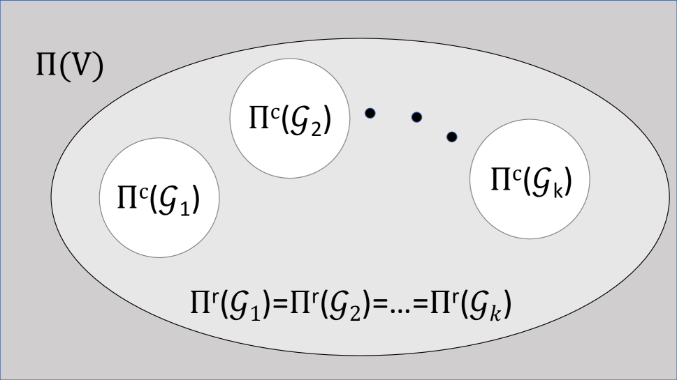
Figure 1: In this figure, $\{\mathcal{G}_{1},\cdots,\mathcal{G}_{k}\}$ denotes a set of Markov equivalent DAGs. $\Pi(\mathbf{V})$ denotes the set of orders over $\mathbf{V}$, which is the search space of ordering-based methods. $\Pi^{c}(\mathcal{G}_{i})$ denotes the set of c-orders of $\mathcal{G}_{i}$, the target space of existing ordering-based methods in the literature. $\Pi^{r}(\mathcal{G}_{i})$ denotes the set of r-orders of $\mathcal{G}_{i}$, which is the target space of the proposed methods in this paper.

There are three main classes of algorithms for causal structure learning: constraint-based, score-based, and hybrid methods. Constraint-based methods use the available data from $P_{\mathbf{V}}$ to test for CI relations in the distribution, from which they learn the MEC of $\mathcal{G}$ (Zhang et al. 2011; Spirtes et al. 2000; Colombo et al. 2012; Sun et al. 2007; Zhang et al. 2017). Score-based methods define a score function (e.g., regularized likelihood function or Bayesian information criterion (BIC)) over the space of graphs and search for a structure that maximizes the score function (Zheng et al. 2018; Zhu, Ng, and Chen 2020; Wang et al. 2021). Hybrid methods combine the strength of both constraint-based and score-based methods to improve score-based algorithms by applying constraint-based techniques (Tsamardinos, Brown, and Aliferis 2006).

Under causal sufficiency assumption, the search space of most of the score-based algorithms is the space of DAGs, which contain $2^{\Omega(n^{2})}$ members when there are $n$ variables in the system. In score-based methods, a variety of search strategies are proposed to solve the maximization problem. Teyssier and Koller (Teyssier and Koller 2005) introduced the first ordering-based search strategy to solve the score-based optimization. The search space of such ordering-based methods is the space of orders over the vertices of the DAG, which includes $2^{\mathcal{O}(n\log(n))}$ orders. Note that the space of orders is significantly smaller than the space of DAGs. Ordering-based methods such as (Zhu, Ng, and Chen 2020; Larranaga et al. 1996; Teyssier and Koller 2005; Friedman and Koller 2003), divide the learning task into two stages. In the first stage, they use the available data to find a causal order (c-order) over the set vertices of $\mathcal{G}$. They use the learned order in the second stage to identify the MEC of $\mathcal{G}$.

All the aforementioned ordering-based approaches for causal discovery require causal sufficiency. In practice, presence of unobserved variables is more the norm rather than the exception. In such cases, instead of a DAG, graphical models such as maximal ancestral graph (MAG) and inducing path graph (IPG) are developed in the literature to represent a causal model (Mokhtarian et al. 2021; Zhang et al. 2019; Rahman et al. 2021). We introduce a novel type of order for MAGs, called removable order (in short, r-order), and argue that r-orders are advantageous over c-orders for structure learning. For one, as r-orders are defined for MAGs (as opposed to DAGs), they can be used to design algorithms for causal graph structure discovery in the absence of causal sufficiency. Moreover, even in the absence of latent variables, r-orders are better suited for learning the MEC. This is because, as depicted in Figure 1, r-orders include c-orders. As a consequence, the problem of searching for an r-order is easier than finding a c-order as the search space remains the same, but the set of feasible solutions is larger.

Our main contributions are summarized as follows.

1. We introduce a novel type of order for MAGs, called r-order, which are invariant among the MAGs in a MEC (Proposition 2). In the case of DAGs, we note that this property does not hold for c-orders as they are mutually exclusive across the graphs in a MEC (Figure 1).

2. We propose ordering-based approaches for identifying the MEC of a MAG using r-orders. In particular, our methods do not require causal sufficiency. Furthermore, we show that the problem of finding an r-order can be cast as a minimization problem and prove that r-orders are the unique minimizers of this problem (Theorem 2).

3. We show that our minimization problem can be formulated with appropriately defined costs as a reinforcement learning problem. Accordingly, any reinforcement learning algorithm can be applied to find a solution for our problem. Additionally, we propose a hill-climbing search algorithm to approximate the solution of the optimization problem of our interest.

Related Work

Under causal sufficiency assumption, several causal structure discovery approaches have been proposed in the literature: constraint-based (Spirtes et al. 2000; Margaritis and Thrun 1999; Pellet and Elisseeff 2008b; Mokhtarian et al. 2021; Tsamardinos, Aliferis, and Statnikov 2003; Sun et al. 2007; Mokhtarian et al. 2022), score-based (Nandy, Hauser, and Maathuis 2018; Zheng et al. 2018; Bottou et al. 2013; Yu et al. 2019), and hybrid (Nandy, Hauser, and Maathuis 2018; Gámez, Mateo, and Puerta 2011; Schulte et al. 2010; Schmidt et al. 2007; Alonso-Barba et al. 2013). Some score-based methods such as (Yu et al. 2019; Lachapelle et al. 2020; Ng et al. 2022; Zheng et al. 2020) formulate the structure learning problem as a smooth continuous optimization and exploit gradient descent to solve it. In (Zhu, Ng, and Chen 2020; Wang et al. 2021), the optimization problem is formulated as a reinforcement learning problem, where the score function is defined over DAGs in (Zhu, Ng, and Chen 2020) and over orders in (Wang et al. 2021). Furthermore, among score-based approaches, various ordering-based methods such as (Zhu, Ng, and Chen 2020; Larranaga et al. 1996; Teyssier and Koller 2005; Friedman and Koller 2003) have been proposed that exploit different search strategies to find a c-order. All of these ordering-based approaches are heuristics and provide no guarantees to finding a correct c-order.

There are a few papers in the literature that do not require causal sufficiency. FCI (Spirtes et al. 2000) is a constraint-based algorithm that starts with the skeleton of the graph learned by PC algorithm and then performs more CI tests to learn a MAG up to its MEC. RFCI (Colombo et al. 2012), FCI+ (Claassen, Mooij, and Heskes 2013), and MBCS*(Pellet and Elisseeff 2008a) are three modifications of FCI. L-MARVEL (Akbari et al. 2021) is a recursive algorithm that iteratively eliminates specific variables and learns the skeleton of a MAG. M3HC (Tsirlis et al. 2018) is a hybrid method that can learn a MAG up to its MEC. To the best of our knowledge, the only other work in the literature that uses an ordering-based approach for causal discovery in MAGs (i.e., in the presence of latent variable) is GSPo which proposes a greedy algorithm that is only consistent as long as there are no latent variables in the system (the graph is a DAG) (Raskutti and Uhler 2018), but there are no theoretical guarantees in case of MAGs (Bernstein et al. 2020).

Preliminary and Problem Description

Throughout the paper, we denote random variables by capital letters (e.g., $X$) and sets of variables by bold letters (e.g., $\mathbf{X}$). A mixed graph (MG) is a graph $\mathcal{G}=(\mathbf{V},\mathbf{E}_{1},\mathbf{E}_{2})$, where $\mathbf{V}$ is a set of vertices, $\mathbf{E}_{1}$ is a set of directed edges, i.e., $\mathbf{E}_{1}\subseteq\{(X,Y)\mid X,Y\in\mathbf{V}\}$, and $\mathbf{E}_{2}$ is a set of bidirected edges, i.e., $\mathbf{E}_{2}\subseteq\{\{X,Y\}\mid X,Y\in\mathbf{V}\}$. For a subset $\mathbf{Z}\subseteq\mathbf{V}$, MG $\mathcal{G}[\mathbf{Z}]=(\mathbf{Z},\mathbf{E}_{1}^{\mathbf{Z}},\mathbf{E}_{2}^{\mathbf{Z}})$ denotes the induced subgraph of $\mathcal{G}$ over $\mathbf{Z}$, that is $\mathbf{E}_{1}^{\mathbf{Z}}=\{(X,Y)\in\mathbf{E}_{1}\mid X,Y\in\mathbf{Z}\}$ and $\mathbf{E}_{2}^{\mathbf{Z}}=\{\{X,Y\}\in\mathbf{E}_{2}\mid X,Y\in\mathbf{Z}\}$. For each directed edge $(X,Y)$ in $\mathbf{E}_{1}$, we say $X$ is a parent of $Y$ and $Y$ is a child of $X$. Further, we say $X$ and $Y$ are neighbors if a directed or undirected edge exists between them in $\mathcal{G}$. The skeleton of $\mathcal{G}$ is the undirected graph obtained by removing the directions of the edges of $\mathcal{G}$. A path $(X_{1},X_{2},\cdots\!,X_{k})$ in $\mathcal{G}$ is called a directed path from $X_{1}$ to $X_{k}$ if $(X_{i},X_{i+1})\in\mathbf{E}_{1}$ for all $1\leq i<k$. If a directed path exists from $X$ to $Y$, $X$ is called an ancestor of $Y$. We denote the set of parents, children, and ancestors of $X$ in $\mathcal{G}$ by $\textit{Pa}_{\mathcal{G}}(X)$, $\textit{Ch}_{\mathcal{G}}(X)$, and $\textit{Anc}_{\mathcal{G}}(X)$, respectively. We also apply these definitions disjunctively to sets of variables, e.g., $\textit{Anc}_{\mathcal{G}}(\mathbf{X})=\bigcup_{X\in\mathbf{X}}\textit{Anc}_{\mathcal{G}}(X)$. A non-endpoint vertex $X_{i}$ on a path $(X_{1},X_{2},\cdots,X_{k})$ is called a collider, if one of the following situations arises.

$$X_{i-1}\to X_{i}\leftarrow X_{i+1},\quad X_{i-1}\leftrightarrow X_{i}\leftarrow X_{i+1},$$

$$X_{i-1}\to X_{i}\leftrightarrow X_{i+1},\quad X_{i-1}\leftrightarrow X_{i}\leftrightarrow X_{i+1}.$$

A path $\mathcal{P}=(X,W_{1},\cdots,W_{k},Y)$ between two distinct variables $X$ and $Y$ is said to be blocked by a set $\mathbf{Z}\subseteq\mathbf{V}\setminus\{X,Y\}$ in $\mathcal{G}$ if there exists $1\leq i\leq k$ such that (i) $W_{i}$is a collider on $\mathcal{P}$ and $W_{i}\notin\textit{Anc}_{\mathcal{G}}(\mathbf{Z}\cup\{X,Y\})$, or (ii) $W_{i}$is not a collider on $\mathcal{P}$ and $W_{i}\in\mathbf{Z}$. We say $\mathbf{Z}$ m-separates $X$ and $Y$ in $\mathcal{G}$ and denote it by $(X\perp\!\!\!\perp Y|\mathbf{Z})_{\mathcal{G}}$ if all the paths in $\mathcal{G}$ between $X$ and $Y$ are blocked by $\mathbf{Z}$.

A directed cycle exists in an MG $\mathcal{G}=(\mathbf{V},\mathbf{E}_{1},\mathbf{E}_{2})$ when there exists $X,Y\in\mathbf{V}$ such that $(X,Y)\in\mathbf{E}_{1}$ and $Y\in\textit{Anc}_{\mathcal{G}}(X)$. Similarly, an almost directed cycle exists in $\mathcal{G}$ when there exists $X,Y\in\mathbf{V}$ such that $\{X,Y\}\in\mathbf{E}_{2}$ and $Y\in\textit{Anc}_{\mathcal{G}}(X)$. An MG with no directed cycles or almost-directed cycles is said to be ancestral. An ancestral MG is called maximal if every pair of non-neighbor vertices are m-separable, i.e., there exists a set of vertices that m-separates them. An MG is called a maximal ancestral graph (MAG) if it is both ancestral and maximal. A MAG with no bidirected edges is called a directed acyclic graph (DAG). Two MAGs $\mathcal{G}_{1}$ and $\mathcal{G}_{2}$ are Markov equivalent if they impose the same set of m-separations, i.e., $(X\perp\!\!\!\perp Y|\mathbf{Z})_{\mathcal{G}_{1}}\iff(X\perp\!\!\!\perp Y|\mathbf{Z})_{\mathcal{G}_{2}}$. We denote by $[\mathcal{G}]$ the Markov equivalence class (MEC) of MAG $\mathcal{G}$, i.e., the set of Markov equivalent MAGs of $\mathcal{G}$. Moreover, if $\mathcal{G}$ is a DAG, we denote by $[\mathcal{G}]^{\text{DAG}}$ the set of Markov equivalent DAGs of $\mathcal{G}$.

Let $\mathcal{G}=(\mathbf{V},\mathbf{E}_{1},\mathbf{E}_{2})$ and $P_{\mathbf{V}}$ denote a MAG and a joint distribution over set of vertices $\mathbf{V}$, respectively. For two distinct variables $X$ and $Y$ in $\mathbf{V}$ and a subset $\mathbf{Z}\subseteq\mathbf{V}\setminus\{X,Y\}$, if $P(X,Y\mid\mathbf{Z})=P(X\mid\mathbf{Z})P(Y\mid\mathbf{Z})$, then $X$ and $Y$ are said be conditionally independent given $\mathbf{Z}$ and it is denoted by $(X\perp\!\!\!\perp Y|\mathbf{Z})_{P_{\mathbf{V}}}$. A Conditional Independence (CI) test refers to detecting whether $(X\perp\!\!\!\perp Y|\mathbf{Z})_{P_{\mathbf{V}}}$. MAG $\mathcal{G}$ satisfies faithfulness w.r.t. (is faithful to) $P_{\mathbf{V}}$ if m-separations in $\mathcal{G}$ is equivalent to CIs in $P_{\mathbf{V}}$, i.e.,

$$(X\perp\!\!\!\perp Y|\mathbf{Z})_{\mathcal{G}}\iff(X\perp\!\!\!\perp Y|\mathbf{Z})_{P_{\mathbf{V}}}.$$

Problem Description:

Consider a set of variables $\mathbf{V}\cup\mathbf{U}$, where $\mathbf{V}$ and $\mathbf{U}$ denote the set of observed and unobserved variables, respectively. In a structural equation model (SEM), each variable $X\in\mathbf{V}\cup\mathbf{U}$ is generated as $X=f_{X}(\textit{Pa}(X),\epsilon_{X})$, where $f_{X}$ is a deterministic function, $\textit{Pa}(X)\subseteq\mathbf{V}\cup\mathbf{U}\setminus\{X\}$, and $\epsilon_{X}$ is the exogenous variable corresponding to $X$ with an additional assumption that the exogenous variables are jointly independent (Pearl 2009). The causal graph of an acyclic SEM is a directed acyclic graph (DAG) over $\mathbf{V}\cup\mathbf{U}$ obtained by adding a directed edge from each variable in $\textit{Pa}(X)$ to $X$, for $X\in\mathbf{V}\cup\mathbf{U}$. The latent projection of this DAG over $\mathbf{V}$ is a MAG over $\mathbf{V}$ such that for $X,Y\in\mathbf{V}$ and $\mathbf{Z}\subseteq\mathbf{V}\setminus\{X,Y\}$, we have

$$(X\perp\!\!\!\perp Y|\mathbf{Z})_{\text{DAG}}\iff(X\perp\!\!\!\perp Y|\mathbf{Z})_{\text{MAG}}.$$

For more details regarding the latent projection, please refer to (Verma and Pearl 1991; Akbari et al. 2021). Let us denote by $\mathcal{G}$ the resulting MAG over $\mathbf{V}$. In this paper, we assume faithfulness, i.e.,

$$(X\perp\!\!\!\perp Y|\mathbf{Z})_{P_{\mathbf{V}}}\iff(X\perp\!\!\!\perp Y|\mathbf{Z})_{\mathcal{G}}.$$

The assumption of causal sufficiency refers to assuming that $\mathbf{U}=\varnothing$. Note that with causal sufficiency, $\mathcal{G}$ is a DAG.

The problem of causal discovery refers to identifying the MEC of $\mathcal{G}$ using samples from the observational distribution. We propose three methods for identifying MEC $[\mathcal{G}]$ using a finite set of samples from $P_{\mathbf{V}}$. It is noteworthy that our proposed methods do not require causal sufficiency.

Ordering-based Methods: Removable Orders vs Causal Orders

In this section, we first define orders and c-orders. Then, we introduce our novel order, r-order, and provide some of its appealing properties.

Definition 1 (order).

An $n$-tuple $(X_{1},\cdots,X_{n})$ is called an order over a set $\mathbf{V}$ if $|\mathbf{V}|=n$ and $\mathbf{V}=\{X_{1},\cdots,X_{n}\}$. We denote by $\Pi(\mathbf{V})$, the set of all orders over $\mathbf{V}$.

Definition 2 (c-order).

An order $(X_{1},\!\cdots\!,X_{n})\in\Pi(\mathbf{V})$ is called a causal order (in short c-order) of a DAG $\mathcal{G}\!=\!(\mathbf{V},\mathbf{E}_{1},\varnothing)$ if $i\!>\!j$ for each $(X_{i},X_{j})\in\mathbf{E}_{1}$. We denote by $\Pi^{c}(\mathcal{G})$ the set of c-orders of $\mathcal{G}$.

Consider the two DAGs $\mathcal{G}_{1}$ and $\mathcal{G}_{2}$ and their sets of c-orders depicted in Figure 2. In this case, $\mathcal{G}_{1}$ and $\mathcal{G}_{2}$ are Markov equivalent and together form a MEC. Furthermore, $\Pi^{c}(\mathcal{G}_{1})$ and $\Pi^{c}(\mathcal{G}_{2})$ are disjoint and each contain 2 orders.

As mentioned earlier, nearly all existing ordering-based methods assume causal sufficiency. These methods divide the learning task into two stages. In the first stage, they search in $\Pi(\mathbf{V})$ (which we refer to as the search space) to find an order in $\Pi^{c}(\mathcal{G})$ (which we refer to as the target space). In the second stage, they use the discovered order to identify MEC $[\mathcal{G}]^{\text{DAG}}$.

(a) DAG $\mathcal{G}_{1}$,
$\Pi^{c}(\mathcal{G}_{1})=\{(X_{1},X_{2},X_{3},X_{4}),$ 
$(X_{1},X_{2},X_{4},X_{3})\}$.

(b) DAG $\mathcal{G}_{2}$,
$\Pi^{c}(\mathcal{G}_{2})=\{(X_{2},X_{1},X_{3},X_{4}),\,$
$(X_{2},X_{1},X_{4},X_{3})\}$.

Figure 2: Two Markov equivalent DAGs $\mathcal{G}_{1}$ and $\mathcal{G}_{2}$ that form a MEC together and their disjoint sets of c-orders. In this example, any order over $\mathbf{V}=\{X_{1},X_{2},X_{3},X_{4}\}$ is an r-order, i.e., $\Pi^{r}(\mathcal{G}_{1})=\Pi^{r}(\mathcal{G}_{2})=\Pi(\mathbf{V})$. Note that $|\Pi^{r}(\mathcal{G}_{1})|=|\Pi^{r}(\mathcal{G}_{2})|=24>2=|\Pi^{c}(\mathcal{G}_{1})|=|\Pi^{c}(\mathcal{G}_{2})|$.

Next, we show that different DAGs in a MEC have a disjoint set of c-orders. In other words, c-orders are not invariant among the DAGs in a MEC. Note that detailed proofs appear in the appendix.

Proposition 1.

Let $\mathcal{G}$ denotes a DAG with MEC $[\mathcal{G}]^{\text{DAG}}=\{\mathcal{G}_{1},...,\mathcal{G}_{k}\}$. For any two distinct DAGs $\mathcal{G}_{i}$ and $\mathcal{G}_{j}$ in $[\mathcal{G}]^{\text{DAG}}$, we have $\Pi^{c}(\mathcal{G}_{i})\cap\Pi^{c}(\mathcal{G}_{j})=\varnothing$.

Removable Orders

In this section, we propose a novel set of orders over the vertices of a MAG, called removable order (in short r-order), and show that r-orders are advantageous for structure learning. First, we review the notion of a removable variable in a MAG, which was recently proposed in the structure learning literature (Mokhtarian et al. 2021, 2022; Akbari et al. 2021).

Definition 3 (removable variable).

Suppose $\mathcal{G}=(\mathbf{V},\mathbf{E}_{1},\mathbf{E}_{2})$ is a MAG. A variable $X\in\mathbf{V}$ is called removable in $\mathcal{G}$ if $\mathcal{G}$ and $\mathcal{G}[\mathbf{V}^{\prime}]$ impose the same set of m-separation relations over $\mathbf{V}^{\prime}$, where $\mathbf{V}^{\prime}=\mathbf{V}\setminus\{X\}$. That is, for any variables $Y,W\in\mathbf{V}^{\prime}$ and $\mathbf{Z}\subseteq\mathbf{V}^{\prime}\setminus\{Y,W\}$,

$$(Y\perp\!\!\!\perp W|\mathbf{Z})_{\mathcal{G}}\iff(Y\perp\!\!\!\perp W|\mathbf{Z})_{\mathcal{G}[\mathbf{V}^{\prime}]}.$$

Below, we introduce the notion of r-order.

Definition 4 (r-order).

An order $\pi=(X_{1},\cdots,X_{n})$ over set $\mathbf{V}$ is called a removable order (r-order) of a MAG $\mathcal{G}=(\mathbf{V},\mathbf{E}_{1},\mathbf{E}_{2})$ if $X_{i}$ is a removable variable in $\mathcal{G}[\{X_{i},\cdots,X_{n}\}]$ for each $1\leq i\leq n$. We denote by $\Pi^{r}(\mathcal{G})$ the set of r-orders of $\mathcal{G}$.

Back to the example in Figure 2 where $\mathcal{G}_{1}$ and $\mathcal{G}_{2}$ are two Markov equivalent DAGs. In this case, any order over the set of vertices is an r-order for both $\mathcal{G}_{1}$ and $\mathcal{G}_{2}$. Hence, each graph has 24 r-orders.

In general, all MAGs in a MEC have the same set of r-orders. Furthermore, in DAGs, r-orders include all the c-orders as subsets (See Figure 1). The following propositions formalize these assertions.

Proposition 2.

If $\mathcal{G}_{1}$ and $\mathcal{G}_{2}$ are two Markov equivalent MAGs, then $\Pi^{r}(\mathcal{G}_{1})=\Pi^{r}(\mathcal{G}_{2})$.

Proposition 3.

For any DAG $\mathcal{G}$, we have $\Pi^{c}(\mathcal{G})\subseteq\Pi^{r}(\mathcal{G})$.

In light of the above propositions, we can summarize some clear advantages of r-orders as follows:

(i) Implication of Proposition 2 is that, unlike c-ordering-based methods, which fail to find a c-order consistent with all the DAGs within a MEC (Proposition 1), r-ordering-based methods can find an order which is an r-order for all the MAGs in its corresponding MEC.

(ii) Proposition 3 implies that in DAGs, the space of r-orders is in general bigger than the space of c-orders. Hence, the target space of an r-ordering-based method is larger than the target space of a c-ordering-based method. For instance, in Figure 2, a c-ordering-based method must find one of the two c-orders of either $\mathcal{G}_{1}$ or $\mathcal{G}_{2}$, while an r-ordering-based method can find any of the 24 r-orders in $\Pi^{r}(\mathcal{G}_{1})=\Pi^{r}(\mathcal{G}_{2})$.

(iii) Since r-orders are defined for MAGs (instead of DAGs), they could be used in ordering-based structure learning approaches without requiring causal sufficiency.

Learning an R-order

In this section, we describe our approach for learning an r-order of the MAGs in $[\mathcal{G}]$. Recall that all MAGs in $[\mathcal{G}]$ have the same set of r-orders. We first propose an algorithm that constructs an undirected graph $\mathcal{G}^{\pi}$ corresponding to an arbitrary order $\pi\in\Pi(\mathbf{V})$. Subsequently, we assign a cost to an order $\pi$ based on the constructed graph $\mathcal{G}^{\pi}$, which is simply the number of edges in $\mathcal{G}^{\pi}$, and show that finding an r-order for $[\mathcal{G}]$ can be cast as an optimization problem with the aforementioned cost. Then, we propose three algorithms to solve the optimization problem.

1:  Function LearnGPi ($\pi,\,\textit{Data}(\mathbf{V})$)

2:  $\mathbf{V}_{1}\leftarrow\mathbf{V}$, $\mathbf{E}^{\pi}\leftarrow\varnothing$

3:  for $t=1$ to $|\mathbf{V}|-1$ do

4:     $X_{t}\leftarrow\pi(t)$

5:     $\mathbf{N}_{X_{t}}\leftarrow\textbf{FindNeighbors}(X_{t},\,\textit{Data}(\mathbf{V}_{t}))$

6:     Add undirected edges between $X_{t}$ and the variables in $\mathbf{N}_{X_{t}}$ to $\mathbf{E}^{\pi}$.

7:     $\mathbf{V}_{t+1}\leftarrow\mathbf{V}_{t}\setminus\{X\}$

8:  Return $\mathcal{G}^{\pi}=(\mathbf{V},\mathbf{E}^{\pi})$

Algorithm 1 Learning $\mathcal{G}^{\pi}$.

Learning an Undirected Graph From an Order

Algorithm 1 iteratively constructs an undirected graph $\mathcal{G}^{\pi}=(\mathbf{V},\mathbf{E}^{\pi})$ from a given order $\pi\in\Pi(\mathbf{V})$. The inputs of Algorithm 1 are an order $\pi$ over $\mathbf{V}$ and observational data $\textit{Data}(\mathbf{V})$ sampled from a joint distribution $P_{\mathbf{V}}$. The algorithm initializes $\mathbf{V}_{1}$ with $\mathbf{V}$ and $\mathbf{E}^{\pi}$ with the empty set in lines 2 and 3, respectively. Then in lines 4-8, it iteratively selects a variable $X_{t}$ according to the given order $\pi$ (line 5) and calls function FindNeighbors in line 6 to learn a set $\mathbf{N}_{X_{t}}\subseteq\mathbf{V}_{t}\setminus\{X_{t}\}$. Then, the algorithm adds undirected edges to $\mathcal{G}^{\pi}$ to connect $X_{t}$ and its discovered neighbors $\mathbf{N}_{X_{t}}$ (line 7). Finally, it updates $\mathbf{V}_{t+1}$ by removing $X_{t}$ from $\mathbf{V}_{t}$ (line 8) and repeats the process.

The output of function FindNeighbors, i.e., $\mathbf{N}_{X_{t}}$, is the set of variables in $\mathbf{V}_{t}$ that are not m-separable from $X_{t}$ using the variables in $\mathbf{V}_{t}$. Hence, if MAG $\mathcal{G}[\mathbf{V}_{t}]$ is faithful to $P_{\mathbf{V}_{t}}$, then $N_{X_{t}}$ would be the set of neighbors of $X_{t}$ among the variables in $\mathbf{V}_{t}$. However, since $\pi$ is arbitrary, $\mathcal{G}[\mathbf{V}_{t}]$ is not necessarily faithful to $P_{\mathbf{V}_{t}}$ and therefore, $\mathbf{N}_{X_{t}}$ can include some vertices that are not neighbors of $X_{t}$. There exist several constraint-based algorithms in the literature, such as (Spirtes et al. 2000; Pellet and Elisseeff 2008a; Colombo et al. 2012; Akbari et al. 2021) that are designed to verify whether two given variables are m-separable. Accordingly, FindNeighbors can use any of such algorithms. Please note that unlike the methods in (Mokhtarian et al. 2022; Akbari et al. 2021) where removable variables are discovered in each iteration, Algorithm 1 selects variables according to the given order $\pi$ (line 4).

Cost of an Order

Suppose $\mathcal{G}$ is faithful to $P_{\mathbf{V}}$. It is shown in (Akbari et al. 2021) that omitting a removable variable does not violate faithfulness in the remaining graph. Hence, due to the definition of r-order, if $\pi\in\Pi^{r}(\mathcal{G}$), then after each iteration $t$, MAG $\mathcal{G}[\mathbf{V}_{t}]$ remains faithful to $P_{\mathbf{V}_{t}}$. The next result shows that Algorithm 1 constructs the skeleton of $\mathcal{G}$ correctly if and only if $\pi$ is an r-order of $\mathcal{G}$.

Theorem 1.

Suppose $\mathcal{G}=(\mathbf{V},\mathbf{E}_{1},\mathbf{E}_{2})$ is a MAG and is faithful to $P_{\mathbf{V}}$, and let $\textit{Data}(\mathbf{V})$ be a collection of i.i.d. samples from $P_{\mathbf{V}}$ with a sufficient number of samples to recover the CI relations in $P_{\mathbf{V}}$. Then, we have the following.

• The output of Algorithm 1 (i.e., $\mathcal{G}^{\pi}$) equals the skeleton of $\mathcal{G}$ if and only if $\pi\in\Pi^{r}(\mathcal{G})$.

• For an arbitrary order $\pi$ over set $\mathbf{V}$, $\mathcal{G}^{\pi}$ is a supergraph of the skeleton of $\mathcal{G}$.

Theorem 1 implies that if $\pi\in\Pi^{r}(\mathcal{G})$, then $\mathcal{G}^{\pi}$ is the skeleton of $\mathcal{G}$, and if $\pi\notin\Pi^{r}(\mathcal{G})$, then $\mathcal{G}^{\pi}$ is a supergraph of the skeleton of $\mathcal{G}$ that contains at least one extra edge. Therefore, by defining the cost of an order in $\Pi(\mathbf{V})$ equal to the number of edges in $\mathcal{G}^{\pi}$, r-orders will be the minimizers, which implies the following.

Theorem 2 (Consistency of the score function).

Any solution of the optimization problem

$$\operatorname*{arg\,min}_{\pi\in\Pi(\mathbf{V})}|\mathbf{E}^{\pi}|,$$ (1)

is an r-order, i.e., a member of $\Pi^{r}(\mathcal{G})$. Conversely every member of $\Pi^{r}(\mathcal{G})$ is also a solution of (1).

Next, we propose both exact and heuristic algorithms for solving the above optimization problem.

Algorithmic Approaches to Finding an R-order

In this section, we propose three algorithms for solving the optimization problem in (1).

Hill-climbing Approach (ROL${}_{\text{HC}}$)

1:  Input: $Data(\mathbf{V})$, maxSwap, maxIter

2:  Initialize $\pi\in\Pi(\mathbf{V})$ as discussed in Appendix A.1

3:  $C_{\pi}\leftarrow\textbf{ComputeCost}(\pi,\textit{Data}(\mathbf{V}))$

4:  for  1 to maxIter do

5:     Denote $\pi$ by $(X_{1},\cdots,X_{n})$

6:     $\Pi^{\text{new}}\!\leftarrow\{(X_{1},\cdots X_{a-1},X_{b},X_{a+1},\cdots,\linebreak X_{b-1},X_{a},X_{b+1},\cdots,X_{n})|1\leq b-a\leq\textit{maxSwap}\}$

7:     for $\pi_{\text{new}}\in\Pi^{\text{new}}$ do

8:        $C_{\pi_{\text{new}}}\leftarrow\textbf{ComputeCost}(\pi_{\text{new}},\textit{Data}(\mathbf{V}))$

9:        if $C_{\pi_{\text{new}}}<C_{\pi}$ then

10:           $\pi\leftarrow\pi_{\text{new}}$, $C_{\pi}\leftarrow C_{\pi_{\text{new}}}$

11:           Break go to line 5

12:  Return $\pi$

1:  Function ComputeCost ($\pi,\,\textit{Data}(\mathbf{V})$)

2:  $\mathcal{G}^{\pi}=(\mathbf{V},\mathbf{E}^{\pi})\leftarrow\textbf{LearnGPi}(\pi,\,\textit{Data}(\mathbf{V}))$

3:  Return $|\mathbf{E}^{\pi}|$

Algorithm 2 Hill-climbing approach (ROL${}_{\text{HC}}$)

In Algorithm 2, we propose a hill-climbing approach, called ROL${}_{\text{HC}}$ for finding an r-order. In general, the output of Algorithm 2 is a suboptimal solution to (1) as it takes an initial order $\pi$ and gradually modifies it to another order with less cost, but it is not guaranteed to find a minimizer of (1) by taking such greedy approach. Nevertheless, this algorithm is suitable for practice as it is scalable to large graphs, and also achieves a superior accuracy compared to the state-of-the-art methods (please refer to the experiment section).

Inputs to Algorithm 2 are the observational data $\textit{Data}(\mathbf{V})$ and two parameters maxIter and maxSwap. maxIter denotes the maximum number of iterations before the algorithm terminates, and maxSwap is an upper bound on the index difference of two variables that can get swapped in an iteration (line 6). Initial order $\pi$ in line 2 can be any arbitrary order, but selecting it cleverly will improve the performance of the algorithm. In Appendix A.1, we describe several ideas for selecting the initial order, such as initialization using the output of other approaches. The algorithm computes the cost of $\pi$ (denoted by $C_{\pi}$) in line 3 by calling subroutine ComputeCost which itself calls subroutine LearnGPi (See Algorithm 1). The remainder of the algorithm (lines 4-12) updates $\pi$ iteratively, maxIter number of times. It updates the current order $\pi\!=\!(X_{1},\!\cdots\!,X_{n})$ as follows: first, it constructs a set of orders $\Pi^{\text{new}}\subseteq\Pi(\mathbf{V})$ from $\pi$ by swapping any two variables $X_{a}$ and $X_{b}$ in $\pi$ as long as $1\leq b-a\leq\textit{maxSwap}$. Next, for each $\pi_{\text{new}}\in\Pi^{\text{new}}$, it computes the cost of $\pi_{\text{new}}$ and if it has a lower cost compared to the current order, the algorithm replaces $\pi$ by that order and repeats the process.

In Appendix A.2, we present a slightly modified version of Algorithm 2, called Algorithm 4, which does not compute the cost of an order as in line 8 of Algorithm 2 but rather uses the information of $C_{\pi}$ for computing the cost of the new permutation $C_{\pi_{\text{new}}}$ (using Algorithm 3 also presented in the Appendix A.2). By doing so, Algorithm 4 significantly reduces the computational complexity.

Exact Reinforcement Learning Approach (ROL${}_{\text{VI}}$)

In this section, we show that the optimization problem in (1) can be cast as a reinforcement learning (RL) problem.

Recall the process of recovering $\mathcal{G}^{\pi}$ from a given order $\pi$ in Algorithm 1. This process can be interpreted as a Markov decision process (MDP) in which the iteration index $t$ denotes time, the set of variables $\mathbf{V}$ represents the action space, and the state space is the set of all subsets of $\mathbf{V}$. More precisely, let $s_{t}$ and $a_{t}$ denote the state and the action of the MDP at time/iteration $t$, respectively. In our setting, $s_{t}$ is the remaining variables at time $t$, i.e., $s_{t}=\mathbf{V}_{t}$, and action $a_{t}$ is the variable that is getting removed from $\mathbf{V}_{t}$ in that iteration, i.e., $a_{t}=X_{t}$. Accordingly, the state transition due to action $a_{t}$ is $s_{t+1}=\mathbf{V}_{t}\setminus\{a_{t}\}$. The immediate reward of selecting action $a_{t}$ at state $s_{t}$ will be the negative of the instant cost, that is the number of discovered neighbors for $a_{t}$ by FindNeighbors in line 6 of Algorithm 1, i.e.,

$$r(s_{t},a_{t})=|\textbf{FindNeighbors}(a_{t},\,\textit{Data}(s_{t}))|=-|\mathbf{N}_{a_{t}}|.$$

Since the form of the function $r(s_{t},a_{t})$ is not known, this is an RL as opposed to a classic MDP setting. We denote by $\pi_{\theta}$, a deterministic policy parameterized by $\theta$. That is, for any state $s_{t}$, $a_{t}=\pi_{\theta}(s_{t})$ is an action in $s_{t}$. Accordingly, we modify Algorithm 1 as follows: it gets a policy $\pi_{\theta}$ instead of a permutation $\pi$ as input. Furthermore, it selects $X_{t}$ in line 5 as $X_{t}=\pi_{\theta}(\mathbf{V}_{t})$. Given a policy $\pi_{\theta}$ and the initial state $s_{1}=\mathbf{V}$, a trajectory $\tau=(s_{1},a_{1},s_{2},a_{2},\cdots,s_{n-1},a_{n-1})$ denotes the sequence of states and actions selected by $\pi_{\theta}$. The cumulative reward of this trajectory, denoted by $R(\tau_{\theta})$, is the sum of the immediate rewards.

$$R(\tau_{\theta})=\sum_{t=1}^{n-1}r(s_{t},a_{t})=-\sum_{t=1}^{n-1}|\mathbf{N}_{a_{t}}|.$$

Hence, if we denote the output of this modified algorithm by $\mathcal{G}^{\theta}=(\mathbf{V},\mathbf{E}^{\theta})$, then $R(\tau_{\theta})=-|\mathbf{E}^{\theta}|$. In this case, any algorithm that finds the optimal policy for RL, such as Value iteration (Sutton and Barto 2018) or Q-learning (Watkins and Dayan 1992) can be used to find a minimum-cost policy $\pi_{\theta}$.

Remark 1.

According to the introduced RL setting, value-iteration can be used to find the optimal policy with the time complexity of $\mathcal{O}(n2^{n})$, which is much less than $\mathcal{O}(n!)$ for naively iterating over all orders.

Approximate Reinforcement Learning Approach (ROL${}_{\text{PG}}$)

Although any algorithm suited for RL is capable of finding an optimal deterministic policy for us, the complexity does not scale well as the graph size. Therefore, we advocate searching for a stochastic policy that increases the exploration during the training of an RL algorithm. As discussed earlier, we could exploit stochastic policies parameterized by neural networks to further improve scalability. However, this could come at the price of approximating the optimal solution instead of finding the exact one. In the stochastic setting, an action $a_{t}$ is selected according to a distribution over the remaining variables, i.e., $a_{t}\sim P_{\theta}(\cdot|s_{t}=\mathbf{V}_{t})$, where $\theta$ denotes the parameters of the policy (e.g., the weights used in training of a neural network). In this case, the objective of the algorithm is to minimize the expected total number of edges learned by policy $P_{\theta}(\cdot|s_{t}=\mathbf{V}_{t})$, i.e.,

$$\operatorname*{arg\,max}_{\theta}\mathbb{E}_{\tau_{\theta}\sim P_{\theta}}\big{[}-|\mathbf{E}^{\theta}|\big{]},$$ (2)

where the expectation is taken w.r.t. randomness of the stochastic policy. Many algorithms have been developed in the literature for finding stochastic policies and solving (2). Some examples include Vanilla Policy Gradient (VPG) (Williams 1992), REINFORCE (Sutton et al. 1999),and Deep Q-Networks (DQN) (Mnih et al. 2013).

Second Stage: Identifying the MEC

In the previous section, we proposed three algorithms for finding an r-order $\pi^{*}\in\Pi^{r}(\mathbf{V})$. Recall that our goal in this paper is to identify the MEC $[\mathcal{G}]$ using the available data from $P_{\mathbf{V}}$. To this end, we can recover the skeleton of the MAGs in $[\mathcal{G}]$ by calling Algorithm 1 with input $\pi^{*}$. Moreover, since FindNeighbors finds a separating set for non-neighbor variables of $X_{t}$ in $\mathcal{G}[\mathbf{V}_{t}]$, we can modify Algorithm 1 to further return a set of separating sets for all the non-neighbor variables in MAG $\mathcal{G}$. This information suffices to identify $[\mathcal{G}]$ by maximally orienting the edges using the complete set of orientation rules introduced in (Zhang 2008).

Experiments

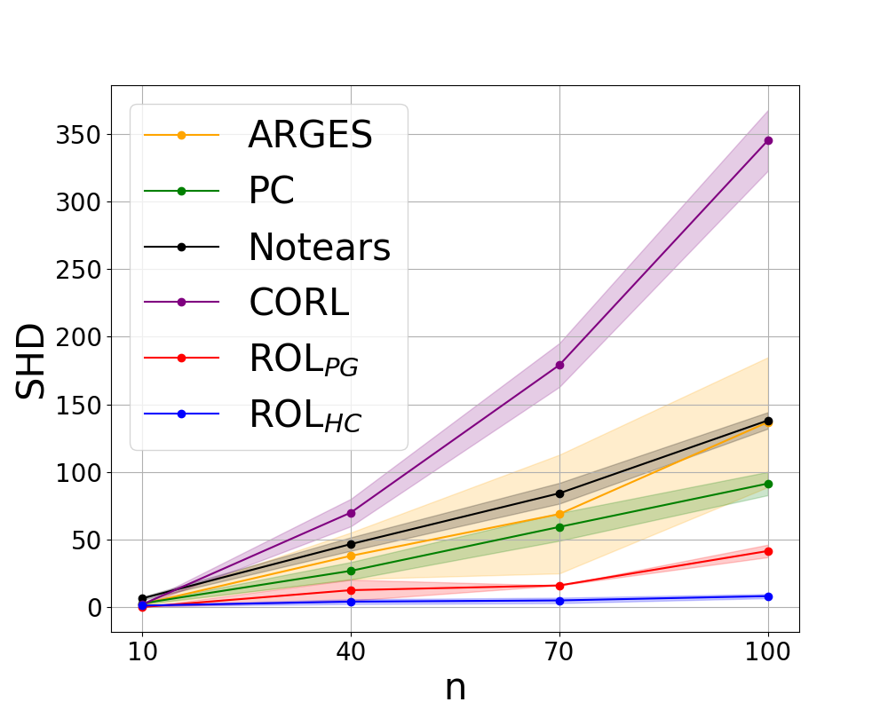
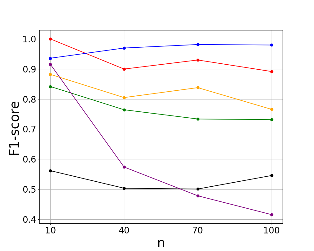
(a) Erdös-Rènyi $Er(n,p=n^{-0.7}),\,\text{sample size}=50n$.

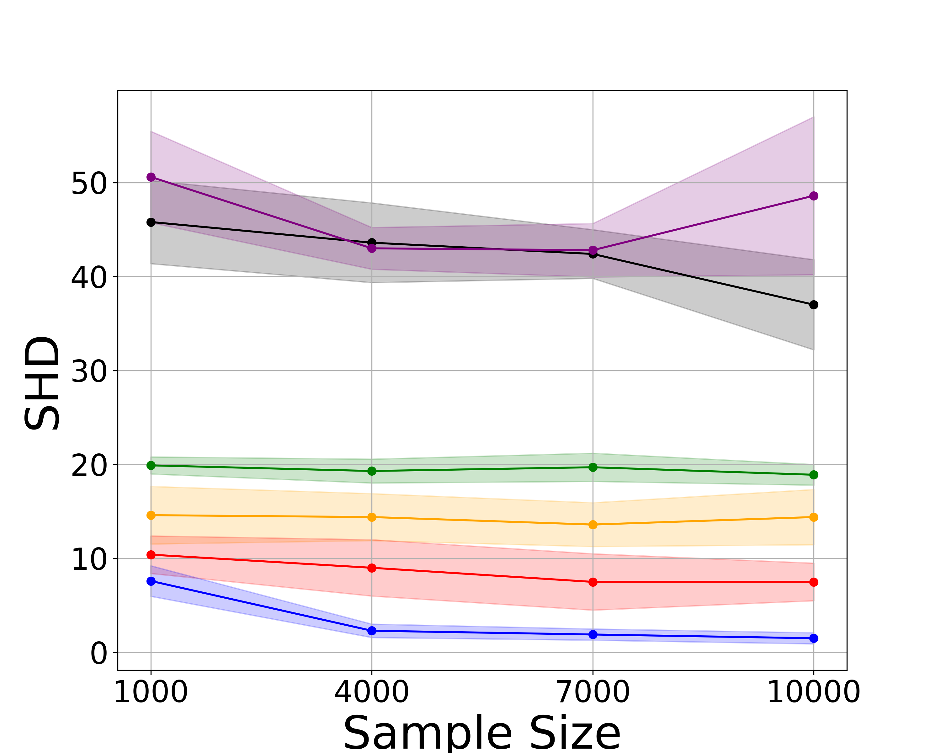
(b) Alarm ($n=37,e=46$).

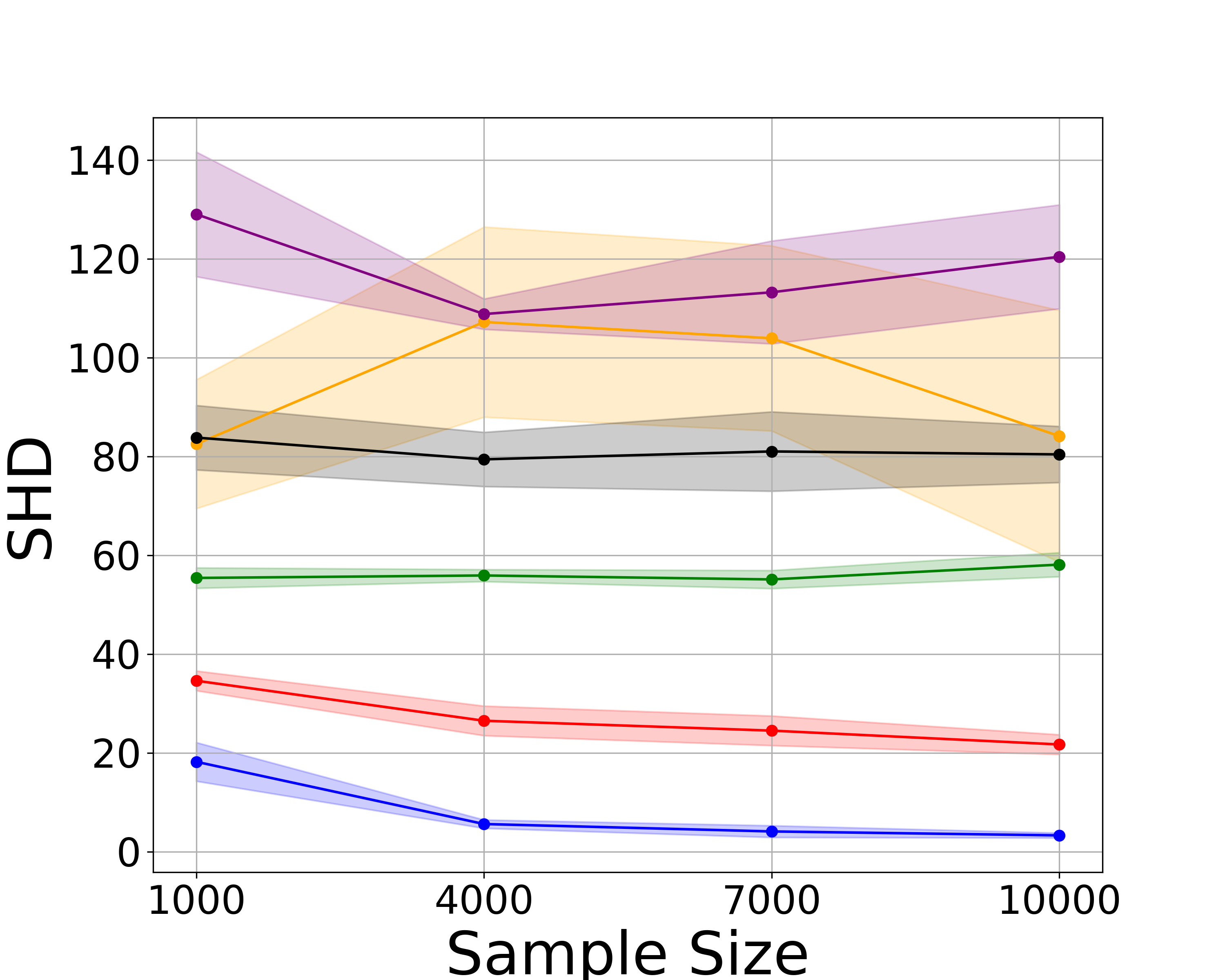
(c) Barley ($n=48,e=84$).

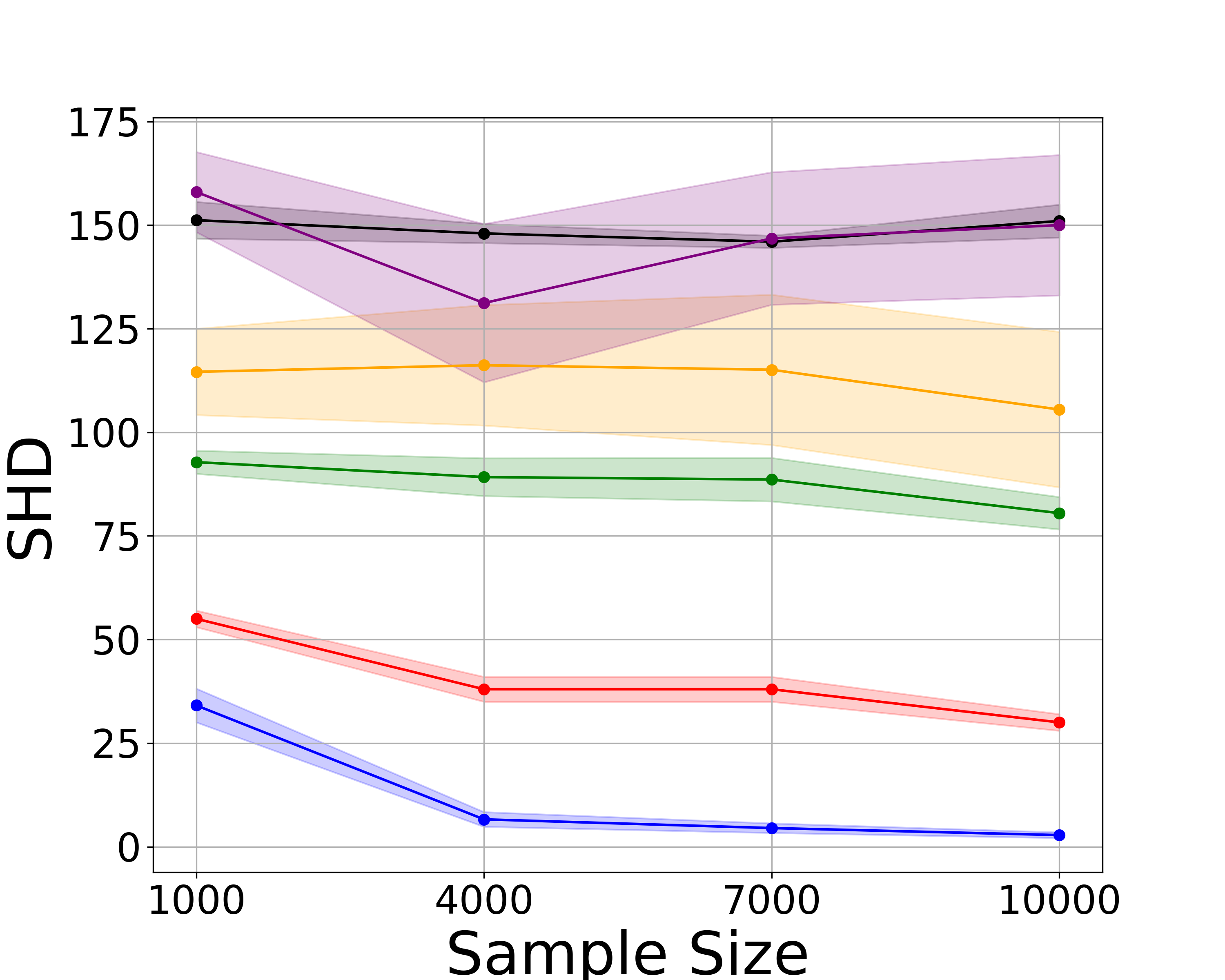
(d) Hepar2 ($n=70,e=123$).

Figure 3: DAG learning; $n$ and $e$ denote the number of variables and the number of edges, respectively.

In this section, we evaluate and compare our algorithms against two types of methods: (i) those assuming causal sufficiency (DAG learning): PC (Spirtes et al. 2000), NOTREARS (Zheng et al. 2018), CORL (Wang et al. 2021), and ARGES (Nandy, Hauser, and Maathuis 2018); (ii) those that do not require causal sufficiency (MAG learning): RFCI (Colombo et al. 2012), FCI+ (Claassen, Mooij, and Heskes 2013), L-MARVEL (Akbari et al. 2021), MBCS* (Pellet and Elisseeff 2008a), and GSPo (Bernstein et al. 2020).

We evaluated the aforementioned algorithms on finite sets of samples, where they were generated using a linear SEM. The coefficients were chosen uniformly at random from $[-1.5,-1]\cup[1,1.5]$; the exogenous noises were generated from normal distribution $\mathcal{N}(0,\sigma^{2})$, where $\sigma$ was selected uniformly at random from $[0.7,1.2]$. We measured the performance of the algorithms by two commonly used metrics in the literature: F1-score and Structural Hamming Distance (SHD) (the discrepancy between the number of extra and missing edges in the learned vs the ground truth graph).

Each point on the plots is reported as the average of 10 runs with 80% confidence interval. Also, each entry in the tables is reported as the average of 10 runs.

DAG Learning

We consider two types of graphs: random graphs generated from Erdös-Rènyi model $Er(n,p)$ and real-world networks. To generate a DAG from $Er(n,p)$, skeleton is first sampled using the Erdös-Rènyi model (Erdős and Rényi 1960) in which undirected edges are sampled independently with probability $p$. Then, the edges are oriented according to a randomly selected c-order.

Figure 3 shows the results for learning DAGs. In Figure 3(a), DAGs are generated from $Er(n,p=n^{-0.7})$ and $n$ varies from 10 to 100. The size of the datasets generated for this part is $50n$. Figures 3(b), 3(c), and 3(d) depict the performance of the algorithms on three real-world structures, called Alarm, Barley, and Hepar2, for a various number of samples. As shown in these figures, ROL${}_{\text{PG}}$ and ROL${}_{\text{HC}}$ outperform the state of the art in both SHD and F1-score metrics.

	Structure		Earthquake	Survey	Asia	Sachs
	$(\#\text{nodes},\#\text{edges})$		(5, 4)	(6, 6)	(8, 8)	(11, 17)
	ROL${}_{\text{VI}}$	F1	0.96	1	0.97	0.97
		SHD	0.4	0	0.4	1
	ROL${}_{\text{HC}}$	F1	0.96	0.98	0.97	0.95
		SHD	0.4	0.2	0.4	1.6

Table 1: Comparing ROL${}_{\text{HC}}$ and ROL${}_{\text{VI}}$ on small graphs.

Table 1 illustrates the performance of ROL${}_{\text{VI}}$ in comparison to ROL${}_{\text{HC}}$ on four small real-world structures. This table shows that ROL${}_{\text{VI}}$ achieves better accuracy on small graphs. Note that ROL${}_{\text{VI}}$ unlike ROL${}_{\text{HC}}$ has theoretical guarantees, but is not scalable to large graphs. However, ROL${}_{\text{VI}}$’s performance is limited to the accuracy of CI tests, and by increasing the dataset sizes, ROL${}_{\text{VI}}$ performs without any errors.

MAG Learning

	Structure		Insurance	Water	Ecoli70	Hailfinder	Carpo	Hepar2	Arth150
	(#Observed, #Unobserved)		(24, 3)	(29, 3)	(43, 3)	(53, 3)	(57, 4)	(65, 5)	(100, 7)
	ROL${}_{\text{HC}}$	F1-score	0.89	0.86	0.93	0.90	1.00	0.97	0.93
		SHD	10.1	18.3	8.1	13.9	0.2	7.6	19.3
	ROL${}_{\text{PG}}$	F1-score	0.86	0.76	0.90	0.87	0.97	0.84	0.93
		SHD	12.9	35.3	12.7	18.4	4.1	36.5	21.5
	RFCI	F1-score	0.74	0.68	0.84	0.84	0.86	0.70	0.86
		SHD	20.5	34.0	17.7	19.7	16.8	52.6	36.3
	FCI+	F1-score	0.60	0.55	0.78	0.77	0.80	0.57	0.78
		SHD	31.2	50.0	23.5	27.2	24.4	81.4	56.7
	L-MARVEL	F1-score	0.87	0.78	0.93	0.90	0.99	0.94	0.92
		SHD	11.5	26.2	8.5	12.8	0.8	12.3	21.2
	MBCS*	F1-score	0.77	0.62	0.90	0.83	0.99	0.92	0.87
		SHD	17.8	38.7	12.0	20.1	1.1	17.0	34.2
	GSPo	F1-score	0.75	0.60	0.66	0.58	0.84	0.58	0.45
		SHD	32.3	89.1	67.6	101.4	31.2	170.6	358.5

Table 2: MAG learning; performance of various algorithms on seven real-world structures, when sample size is $50n$.

We selected seven real-world DAGs for this part. For each structure, we randomly removed $5\%$ to $10\%$ of the variables and constructed a MAG over the set of observed variables (those not eliminated) using the latent projection approach of (Verma and Pearl 1991). Finally, we generated a finite set of samples over all the variables and fed the data pertaining to the observed variables as the input to all the algorithms. The goal of all algorithms is to learn the MEC of the corresponding MAG from the samples they have.

Table 2 presents the results. As demonstrated by the bold entries in the table, ROL${}_{\text{HC}}$ achieves the best F1-score and SHD in almost all the cases.

Remark 2.

Recall that prior to this work, GSPo was the only ordering-based method in the literature that does not require causal sufficiency. However, the table shows that it has the worst performance among the algorithms and is not scalable to large graphs. For instance, it has a poor performance on Arth150, which is a graph with 100 variables.

Conclusion, Limitations, Future work

We advocated for a novel type of order, called an r-order, and argued that r-orders are advantageous over the previously used orders in the literature. Accordingly, we proposed three algorithms for causal structure learning in the presence of unobserved variables: ROL${}_{\text{HC}}$, a Hill-climbing-based heuristic algorithm that is scalable to large graphs; ROL${}_{\text{VI}}$, an exact RL-based algorithm that has theoretical guarantees but is not scalable to large graphs; ROL${}_{\text{PG}}$, an approximate RL-based algorithm that exploits stochastic policy gradient. We showed in our experiments that ROL${}_{\text{VI}}$ on small graphs and ROL${}_{\text{HC}}$ on larger graphs outperform the state-of-the-art algorithms. Although ROL${}_{\text{PG}}$ is scalable to large graphs and outperforms the existing methods, ROL${}_{\text{HC}}$ performs slightly better, mainly due to better initialization. The weights of the neural networks in ROL${}_{\text{PG}}$ are selected randomly, while we proposed clever methods for the initialization step in ROL${}_{\text{HC}}$. Nevertheless, an important future work is to improve the policy gradient approaches.

Appendix

Appendix A A  Implementation of the Hill-climbing Approach

In this section, we discuss some details regarding implementing our hill-climbing approach. In Section A.1, we introduce three ways to initialize $\pi$ in line 2 of Algorithm 2. In Section A.2, we present a slightly modified version of Algorithm 2 which does not compute the cost of an order as in line 8 of Algorithm 2 but rather uses the information of $C_{\pi}$ for computing the cost of the new permutation $C_{\pi_{\text{new}}}$.

A.1  Initialization in Line 2 of Algorithm 2

Random Permutation:

This is a naive approach in which we select the initial order randomly from $\Pi(\mathbf{V})$.

Sort by the Size Markov Boundary:

The Markov boundary of a variable is defined in the following.

Definition 5 (Markov boundary).

Markov boundary of $X\in\mathbf{V}$, denoted by $\textit{Mb}_{\mathbf{V}}(X)$, is a minimal set of variables $\mathbf{Z}\subseteq\mathbf{V}\setminus\{X\}$, such that $X$ is independent of the rest of the variables of $\mathbf{V}$ conditioned on $\mathbf{Z}$.

There exist several algorithms in the literature for discovering the Markov boundaries (Margaritis and Thrun 1999; Pellet and Elisseeff 2008b). For instance, TC (Pellet and Elisseeff 2008b) algorithm proves that $X$ and $Y$ are in each other’s Markov boundary if and only if

$$(X\not\!\perp\!\!\!\perp Y|\mathbf{V}\setminus\{X,Y\})_{P_{\mathbf{V}}}.$$

The following lemma shows that removable variables have a small Markov boundary size.

Lemma 1 (Lemma 3 in (Akbari et al. 2021)).

If $X$ is removable in $\mathcal{G}$, then for every $Y\in\textit{Mb}_{\mathbf{V}}(X)$, we have

$$\textit{Mb}_{\mathbf{V}}(X)\subseteq\textit{Mb}_{\mathbf{V}}(Y).$$ (3)

Motivated by this lemma, we initialize $\pi$ by the sorting of $\mathbf{V}$ based on the Markov boundary size in ascending order. That is, $\pi:=(X_{1},\cdots,X_{n})$, where $\textit{Mb}_{\mathbf{V}}(X_{1})\leq\cdots\leq\textit{Mb}_{\mathbf{V}}(X_{n})$.

A recursive Approaches:

As mentioned in the main text, some recursive approaches have been proposed in the literature of structure learning (Mokhtarian et al. 2021; Akbari et al. 2021; Mokhtarian et al. 2022). These methods identify a removable variable in each iteration by performing a set of CI tests. Herein, we use one of those algorithms and store the order of removed variables. In practice, the CI tests are noisy. Accordingly, their removability test may not be accurate. However, we can use their found order to initialize $\pi$. By doing so, and as illustrated in our experiments, the accuracy of our proposed method is significantly improved.

A.2  Computing the Cost of a New Permutation

Herein, we propose Algorithm 3, an alternative way for computing the cost of an order $\pi=(X_{1},\cdots,X_{n})$ instead of using Algorithm 1 and counting the number of edges in $\mathcal{G}^{\pi}$.

1:  Function ComputeCost ($\pi,\,a,\,b,\,\textit{Data}(\mathbf{V})$)

2:  $\mathbf{V}_{\text{rem}}\leftarrow\mathbf{V}$

3:  $C_{ab}\leftarrow(0,0,\cdots,0)\in\mathbb{R}^{n}$

4:  for $t=a$ to $b$ do

5:     $X\leftarrow\pi(t)$

6:     $\mathbf{N}_{X}\leftarrow\textbf{FindNeighbors}(X,\,\textit{Data}(\mathbf{V}_{\text{rem}}))$

7:     $\mathbf{C}_{ab}(t)\leftarrow|\mathbf{N}_{X}|$

8:     $\mathbf{V}_{\text{rem}}\leftarrow\mathbf{V}_{\text{rem}}\setminus\{X\}$

9:  Return $C_{ab}$

Algorithm 3 Compute cost of an order

This algorithm additionally gets two numbers $1\leq a<b\leq n$ as input and returns a vector $C_{ab}\in\mathbb{R}^{n}$. For $a\leq i\leq b$, the $i$-th entry of $C_{ab}$ is equal to $|N_{X_{i}}|$ which is the number of neighbors of $X_{i}$ in the remaining graph. Hence, to learn the total cost of $\pi$, we can call this function with $a=1$ and $b=n$ and then compute the sum of the entries of the output $C_{1n}$. Accordingly, we modify Algorithm 2 and propose Algorithm 4.

1:  Input: $Data(\mathbf{V})$, maxSwap, maxIter

2:  Initialize $\pi\in\Pi(\mathbf{V})$ as discussed in Appendix A.1

3:  $C_{1n}\leftarrow\textbf{ComputeCost}(\pi,1,n,\textit{Data}(\mathbf{V}))$

4:  for  1 to maxIter do

5:     Denote $\pi$ by $(X_{1},\cdots,X_{n})$

6:     for $1\leq a<b\leq n$ such that $b-a<\text{maxSwap}$ do

7:        $\pi_{\text{new}}\leftarrow$ Swap $X_{a}$ and $X_{b}$ in $\pi$

8:        $C^{\text{new}}_{ab}\leftarrow\textbf{ComputeCost}(\pi_{\text{new}},a,b,\textit{Data}(\mathbf{V}))$

9:        if $\sum_{i=a}^{b}C^{\text{new}}_{ab}(i)<\sum_{i=a}^{b}C_{1n}(i)$ then

10:           $\pi\leftarrow\pi_{\text{new}}$

11:           $C_{1n}(a:b)\leftarrow C^{\text{new}}_{ab}(a:b)$

12:           Break the for loop in line 5

13:  Return $\pi$

Algorithm 4 Modified hill climbing approach

In this algorithm, $C_{1n}$ is a vector that stores the cost of $\pi$, computed in line 3. Similar to Algorithm 2, a new permutation $\pi_{\text{new}}$ is constructed by swapping two entries $X_{a}$ and $X_{b}$ in $\pi$. The main change is in line 8, where the algorithm calls function ComputeCost with $a$ and $b$ to compute the cost of the new policy. The reason is that for $i<a$ and $i>b$, the $i$-th entry of the cost of $\pi$ and $\pi_{\text{new}}$ are the same. This is because the set of remaining variables is the same. Hence, to compare the cost of $\pi$ with the cost of $\pi_{\text{new}}$, it suffices to compare them for entries between $a$ and $b$. Accordingly, Algorithm 4 checks the condition in line 9, and if the cost of the new policy is better, then the algorithm updates $\pi$ and its corresponding cost. Note that it suffices to update the entries between $a$ to $b$ of $C_{1n}$.

Appendix B B  Technical proofs

Proposition 1.

Let $\mathcal{G}$ denotes a DAG with MEC $[\mathcal{G}]^{\text{DAG}}=\{\mathcal{G}_{1},...,\mathcal{G}_{k}\}$. For any two distinct DAGs $\mathcal{G}_{i}$ and $\mathcal{G}_{j}$ in $[\mathcal{G}]^{\text{DAG}}$, we have $\Pi^{c}(\mathcal{G}_{i})\cap\Pi^{c}(\mathcal{G}_{j})=\varnothing$.

Proof.

Let $\mathcal{G}_{i}=(\mathbf{V},\mathbf{E}_{i})$ and $\mathcal{G}_{j}=(\mathbf{V},\mathbf{E}_{j})$ denote two distinct DAGs in $[\mathcal{G}]^{\text{DAG}}$. It is well-known that two Markov equivalent DAGs have the same skeleton (Verma and Pearl 1991). Hence, $\mathcal{G}_{i}$ and $\mathcal{G}_{j}$ have the same skeleton. Moreover, as $\mathcal{G}_{i}$ and $\mathcal{G}_{j}$ are two distinct DAGs, there exist two variables $X$ and $Y$ in $\mathbf{V}$ such that $(X,Y)\in\mathbf{E}_{i}$ and $(Y,X)\in\mathbf{E}_{j}$. Recall that in c-orders, parents of a variable appear after that variable in the order. This implies that in any c-order of $\mathcal{G}_{i}$, $X$ appears after $Y$, but in any c-order of $\mathcal{G}_{j}$, $X$ appears before $Y$. Therefore, the set of c-orders of $\mathcal{G}_{i}$ and $\mathcal{G}_{j}$ do not share any common order, i.e., $\Pi^{c}(\mathcal{G}_{i})\cap\Pi^{c}(\mathcal{G}_{j})=\varnothing$. ∎

Proposition 2.

If $\mathcal{G}_{1}$ and $\mathcal{G}_{2}$ are two Markov equivalent MAGs, then $\Pi^{r}(\mathcal{G}_{1})=\Pi^{r}(\mathcal{G}_{2})$.

Proof.

To prove this proposition, we first provide a corollary of a result in (Akbari et al. 2021).

Corollary 1 (It follows from Theorem 2 in (Akbari et al. 2021)).

For two Markov equivalent MAGs $\mathcal{G}^{1}$ and $\mathcal{G}^{2}$ over $\mathbf{V}$ and an arbitrary variable $X\in\mathbf{V}$, $X$ is removable in $\mathcal{G}^{1}$ if and only if $X$ is removable in $\mathcal{G}^{2}$.

Suppose $\pi=(X_{1},\cdots,X_{n})\in\Pi^{r}(\mathcal{G}_{1})$. It suffices to show that $\pi\in\Pi^{r}(\mathcal{G}_{2})$, i.e., $X_{i}$ is removable in $\mathcal{G}_{2}[\{X_{i},\cdots,X_{n}\}]$ for each $1\leq i\leq n$.

By induction on $i$, we show that $\mathcal{G}_{1}[\{X_{i},\cdots,X_{n}\}]$ and $\mathcal{G}_{2}[\{X_{i},\cdots,X_{n}\}]$ are Markov equivalent. This claim holds for $i=1$ due to the assumption of the proposition. Suppose it holds for an $i<n$ and we want to show that $\mathcal{G}_{1}[X_{i+1},\cdots,X_{n}]$ and $\mathcal{G}_{2}[\{X_{i+1},\cdots,X_{n}\}]$ are Markov equivalent. As $\pi\in\Pi^{r}(\mathcal{G}_{1})$, $X_{i}$ is removable in $\mathcal{G}_{1}[\{X_{i},\cdots,X_{n}\}]$. Furthermore, Corollary 1 implies that $X_{i}$ is also removable in $\mathcal{G}_{2}[\{X_{i},\cdots,X_{n}\}]$. Therefore, for any variables $Y,W\in\{X_{i+1},\cdots,X_{n}\}$ and $\mathbf{Z}\subseteq\{X_{i+1},\cdots,X_{n}\}\setminus\{Y,W\}$, we have

$$(Y\perp\!\!\!\perp W|\mathbf{Z})_{\mathcal{G}_{1}[X_{i},\cdots,X_{n}]}\iff(Y\perp\!\!\!\perp W|\mathbf{Z})_{\mathcal{G}_{1}[X_{i+1},\cdots,X_{n}]},$$ (4)

and

$$(Y\perp\!\!\!\perp W|\mathbf{Z})_{\mathcal{G}_{2}[X_{i},\cdots,X_{n}]}\iff(Y\perp\!\!\!\perp W|\mathbf{Z})_{\mathcal{G}_{2}[X_{i+1},\cdots,X_{n}]}.$$ (5)

Because $\mathcal{G}_{1}[\{X_{i},\cdots,X_{n}\}]$ and $\mathcal{G}_{2}[\{X_{i},\cdots,X_{n}\}]$ are Markov equivalent, they impose the same m-separation relations over $\{X_{i},\cdots,X_{n}\}$. Thus, Equations (4) and (5) imply that $\mathcal{G}_{1}[\{X_{i+1},\cdots,X_{n}\}]$ and $\mathcal{G}_{2}[\{X_{i+1},\cdots,X_{n}\}]$ impose the same m-separation relations over $\{X_{i+1},\cdots,X_{n}\}$, i.e., they are Markov equivalent which proves our claim.

So far, we have shown that $\mathcal{G}_{1}[\{X_{i},\cdots,X_{n}\}]$ and $\mathcal{G}_{2}[\{X_{i},\cdots,X_{n}\}]$ are Markov equivalent for each $1\leq i\leq n$. In this case, for each $1\leq i\leq n$, Corollary 1 implies that $X_{i}$ is removable in $\mathcal{G}_{2}[\{X_{i},\cdots,X_{n}\}]$, because it is removable in $\mathcal{G}_{1}[\{X_{i},\cdots,X_{n}\}]$. This completes the proof. ∎

Proposition 3.

For any DAG $\mathcal{G}$, we have $\Pi^{c}(\mathcal{G})\subseteq\Pi^{r}(\mathcal{G})$.

Proof.

Let $\pi=(X_{1},\cdots,X_{n})$ be an order in $\Pi^{c}(\mathcal{G})$. It suffices to show that $\pi\in\Pi^{r}(\mathcal{G})$ or equivalently, $X_{i}$ is removable in DAG $\mathcal{G}[\{X_{i},\cdots,X_{n}\}]$ for each $1\leq i\leq n$. Let $1\leq i\leq n$ be arbitrary. As $\pi\in\Pi^{c}(\mathcal{G})$, there is no directed edge from $X_{i}$ to the variables in $\{X_{i+1},\cdots,X_{n}\}$. Hence, $X_{i}$ has not child in $\mathcal{G}[\{X_{i},\cdots,X_{n}\}]$. In this case, Remark 6 in (Mokhtarian et al. 2021) proves that $X_{i}$ is removable in DAG $\mathcal{G}[\{X_{i},\cdots,X_{n}\}]$. ∎

Theorem 1.

Suppose $\mathcal{G}=(\mathbf{V},\mathbf{E}_{1},\mathbf{E}_{2})$ is a MAG and is faithful to $P_{\mathbf{V}}$, and let $\textit{Data}(\mathbf{V})$ be a collection of i.i.d. samples from $P_{\mathbf{V}}$ with a sufficient number of samples to recover the CI relations in $P_{\mathbf{V}}$. Then, we have the following.

1. The output of Algorithm 1 (i.e., $\mathcal{G}^{\pi}$) equals the skeleton of $\mathcal{G}$ if and only if $\pi\in\Pi^{r}(\mathcal{G})$.

2. For an arbitrary order $\pi$ over set $\mathbf{V}$, $\mathcal{G}^{\pi}$ is a supergraph of the skeleton of $\mathcal{G}$.

Proof.

We prove the two parts of the theorem separately.

1. Suppose $\mathcal{G}^{1}$ is a MAG over a set $\mathbf{V}^{1}$ that is faithful to a distribution $P_{\mathbf{V}^{1}}$ and let $\mathbf{V}^{2}$ be an arbitrary subset of $\mathbf{V}^{1}$. The latent projection of $\mathcal{G}^{1}$ over $\mathbf{V}^{2}$ is a MAG over $\mathbf{V}^{2}$ that is faithful to $P_{\mathbf{V}^{2}}$. It is well-known that $\mathcal{G}^{2}$ is a supergraph of $\mathcal{G}^{1}$ where some extra edges are added to $\mathcal{G}^{1}$ according to some new unblocked paths, known as inducing paths (Verma and Pearl 1991). Equipped with this definition, (Akbari et al. 2021) provides the following result.

   Lemma 2 (Proposition 1 in (Akbari et al. 2021)).

   Suppose $\mathcal{G}^{1}$ is a MAG over a set $\mathbf{V}^{1}$ that is faithful to $P_{\mathbf{V}^{1}}$. Let $X\in\mathbf{V}^{1}$ be arbitrary and $\mathcal{G}^{2}$ be the latent projection of $\mathcal{G}^{1}$ over $\mathbf{V}^{2}$, where $\mathbf{V}^{2}=\mathbf{V}^{1}\setminus\{X\}$. In this case, MAG $\mathcal{G}^{1}[\mathbf{V}^{2}]$ is equal to $\mathcal{G}^{2}$ if and only if $X$ is removable in $\mathcal{G}^{1}$.

   Using this lemma, we complete the proof in the following.

   Sufficient part: Suppose $\pi=(X_{1},\cdots,X_{n})\in\Pi^{r}(\mathcal{G})$, i.e., $X_{t}$ is removable in $\mathcal{G}[\{X_{t},\cdots,X_{n}\}]$ for each $1\leq t\leq n$. Recall that $\mathbf{V}_{t}=\{X_{t},\cdots,X_{n}\}$ in Algorithm 1. Lemma 2 implies that at each iteration $t$, $\mathcal{G}[\mathbf{V}_{t}]$ is faithful to $P_{\mathbf{V}_{t}}$. In this case, function FindNeighbors correctly learns the neighbors of $X_{t}$ among the remaining variables $\mathbf{V}_{t}$, i.e., $N_{X_{t}}$ is the set of neighbors of $X_{t}$ in $\mathcal{G}[\mathbf{V}_{t}]$. Hence, $\mathcal{G}^{\pi}$ equals the skeleton of $\mathcal{G}$ at the end of the algorithm.

   Necessary part: Suppose $\pi=(X_{1},\cdots,X_{n})\notin\Pi^{r}(\mathcal{G})$, i.e., there exists $1\leq i\leq n$ such that $X_{i}$ is not removable in $\mathcal{G}[\mathbf{V}_{i}]$. Recall that $\mathbf{V}_{i}=\{X_{i},\cdots,X_{n}\}$ and $\mathbf{V}_{i+1}=\mathbf{V}_{i}\setminus\{X_{i}\}$. Let $\mathcal{G}^{1}$ denotes $\mathcal{G}[\mathbf{V}_{i}]$ and $\mathcal{G}^{2}$ denotes the latent projection of $\mathcal{G}^{1}$ on $\mathbf{V}_{i+1}$. In this case, Lemma 2 implies that $\mathcal{G}^{2}$ has some extra edges compared to $\mathcal{G}^{1}[\mathbf{V}_{i+1}]=\mathcal{G}[\mathbf{V}_{i+1}]$. Let $(Y,W)$ be an edge in $\mathcal{G}^{2}$ that is not in $\mathcal{G}[\mathbf{V}_{i+1}]$. In this case, $Y$ and $W$ are not m-separable using the subsets of $\mathbf{V}_{i+1}$. Hence, $\{Y,W\}$ will be added to the learned graph $\mathcal{G}^{\pi}$. Note that this edge does not exist in $\mathcal{G}$, which shows that the learned graph is not equal to the skeleton of $\mathcal{G}$.

2. Let $\pi=\{X_{1},\cdots,X_{n}\}$ and $(X_{a},X_{b})$ be an edge in $\mathcal{G}$. It suffices to show that $\{X_{a},X_{b}\}$ appears in $\mathcal{G}^{\pi}$. When $t=\min(a,b)$ in Algorithm 1, both $X_{a}$ and $X_{b}$ exists in $\mathbf{V}_{t}$. Note that $X_{t}\in\{X_{a},X_{b}\}$. In this case, $X_{a}$ and $X_{b}$ are not m-separable as they are neighbors. Hence, function FindNeighbors identify them as neighbors and therefore, undirected edge $\{X_{a},X_{b}\}$ will be added to $\mathcal{G}^{\pi}$.

∎

Appendix C C  Complementary of the Experiment Section

In this section, we provide additional experiments, discuss details pertaining to the reproducibility and hyper-parameters, formally define the evaluation metrics, illustrate the runtime and discuss the time-complexity of our methods, and present more details about the real-world structures used in our experiments.

C.1  Additional Experiments

Additional Experiments on Random Graphs:

To illustrate the effect of the graph density on the performance of various learning algorithms, in this section, we evaluated several algorithms on randomly generated graphs with a fixed number of vertices and different densities. Figure 4 illustrates the performance of various learning algorithms on random graphs generated from $Er(50,p)$ model when $n=50$ and $p$ varies from $0.04$ to $0.08$. Similar to Figure 2(a) in the main text, ROL${}_{\text{PG}}$ and ROL${}_{\text{HC}}$ outperform the state of the art in both SHD and F1-score metrics.

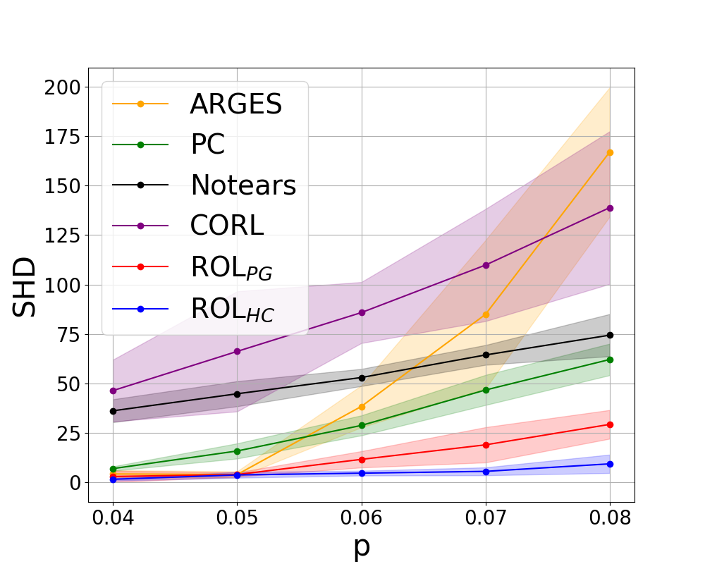
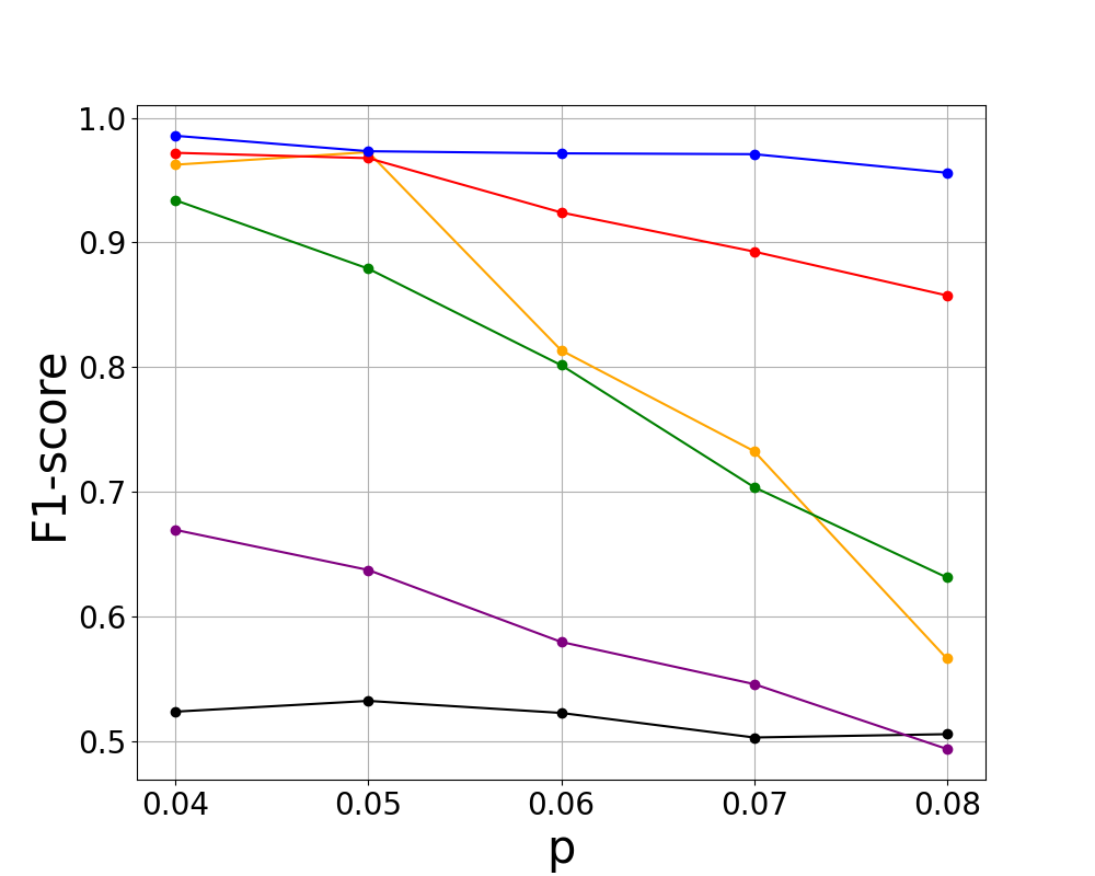
Figure 4: Erdös-Rènyi $Er(n=50,p),\,\text{sample size}=2500$.

ROC Curves

we present the ROC of different methods in Figure 5 for learning the graph of dataset Alarm. This shows that our algorithms have both higher true positive (TP) and lower false positive (FP) rates compared to the others.

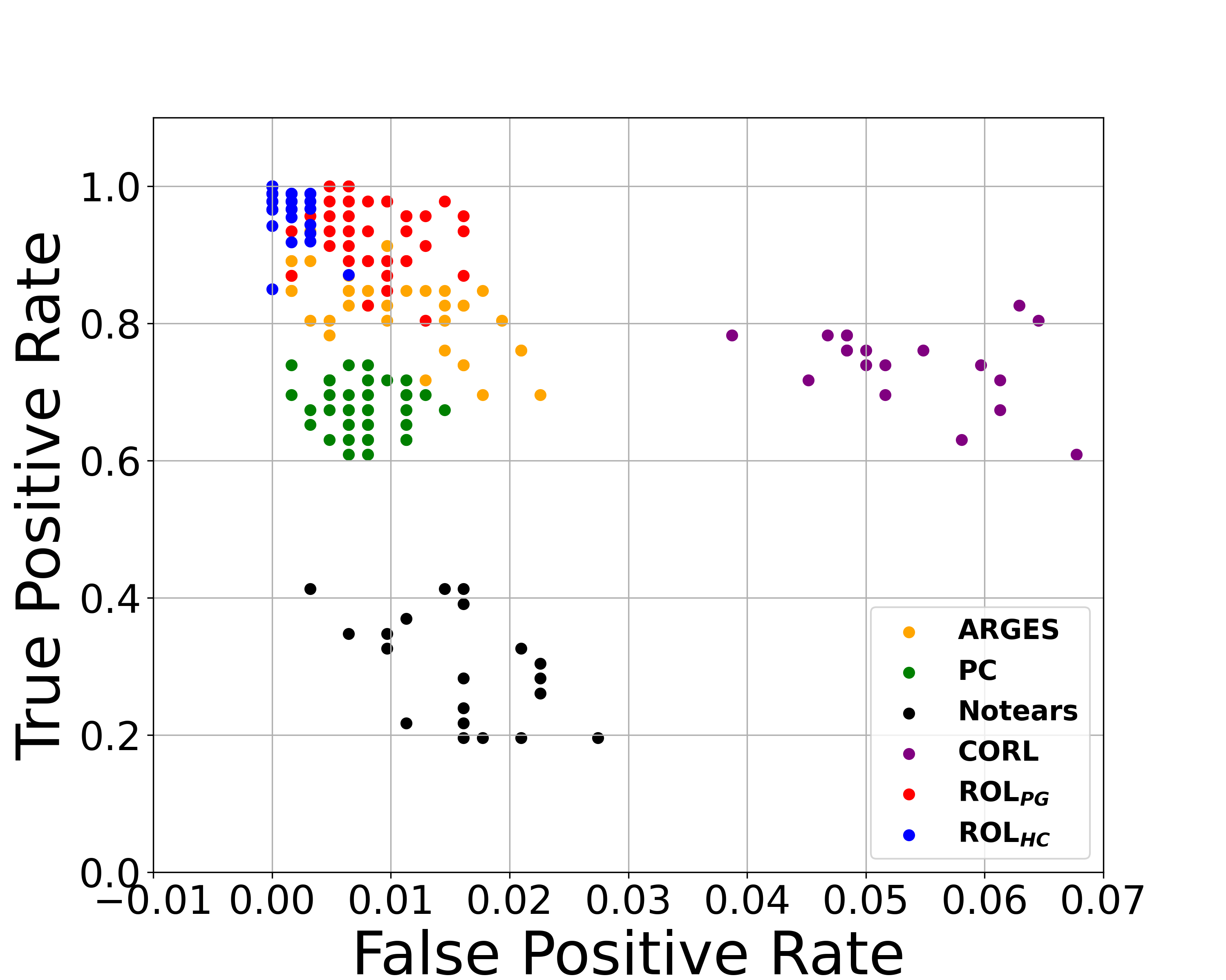
Figure 5: ROC plot of various algorithms for learning graph Alarm.

C.2  Reproducibility and Hyper-parameters

For our experiments, we utilized a Linux server with Intel Xeon CPU E5-2680 v3 (24 cores) operating at 2.50GHz with 256 GB DDR4 of memory and 2x Nvidia Titan X Maxwell GPUs.

Next, we introduce all the details, including hyper-parameters that were used in the implementation of our proposed methods.

ROL${}_{\text{HC}}$:

In our implementation, we used the modified version of our algorithm introduced in Appendix A.2, i.e., Algorithms 3 and 4. We called the algorithms with parameters $\textit{maxIter}=20$ and $\textit{maxSwap}=10$. To initialize $\pi$ in line 2, we used the recursive approach introduced in Appendix A.1 by the method in (Mokhtarian et al. 2022). As discussed in the main text, there are several algorithms in the literature to implement FindNeighbors function. Herein, we used the algorithm in (Mokhtarian et al. 2022) which is reasonably fast for large graphs. To perform CI tests from the available dataset, we used Fisher Z-transformation with a significance level of $\alpha=0.01$. Please note that we repeated almost all the experiments with different $\alpha$, e.g., $\alpha=0.05$, and the results remained very similar to the results for $\alpha=0.01$. Thus, we did not report them separately.

ROL${}_{\text{PG}}$:

For our RL approach, we used Garage library (garage contributors 2019) as it is easy to maintain and parallelize. To this end, we implemented an environment class compatible with Garage library and Softmax Policy. We used an MLP with two hidden layers, each with 64 neurons, and the $\tanh$ activation function for the hidden layers to model the policy function. Afterward, we employed a modified version of the Vanilla Policy Gradient algorithm that allows us to fit a linear feature baseline in order to achieve better performance by reducing the variance (Sutton et al. 1999).

C.3  Evaluation Metrics

As mentioned in the experiment section, we measured the performance of the algorithms by two commonly used metrics in the literature: F1-score and Structural Hamming Distance (SHD). Herein, we formally define these measures.

Let $\mathcal{G}_{1}$ and $\mathcal{G}_{2}$ denote the true graph’s skeleton and the learned graph’s skeleton, respectively. We first define a few notations. True-positive (TP) is the number of edges that appear in both $\mathcal{G}_{1}$ and $\mathcal{G}_{2}$. False-positive (FP) is the number of edges that appear in $\mathcal{G}_{2}$ but do not exist in $\mathcal{G}_{1}$. False-negative (FN) is the number of edges in $\mathcal{G}_{1}$ that the algorithm failed to learn in $\mathcal{G}_{2}$. In this case, SHD is defined as follows.

$$\text{SHD = FP + FN}.$$

To define F1-score, we first define precision and recall in the following.

$$\text{Precision = }\frac{\text{TP}}{\text{TP + FP}}.$$

$$\text{Recall = }\frac{\text{TP}}{\text{TP + FN}}.$$

Finally, F1-score is defined as follows.

$$\text{F1-score = }2\times\frac{\text{Precision }\times\text{ Recall}}{\text{Precision }+\text{ Recall}}.$$

Note that F1-score is a number between 0 to 1, while larger numbers indicate better accuracy.

C.4  Time Complexity and Runtime

We illustrate the runtime of various algorithms in Figure 6 for learning the graph of the dataset Barley. This figure shows that our algorithms are relatively faster than the state-of-the-art methods.

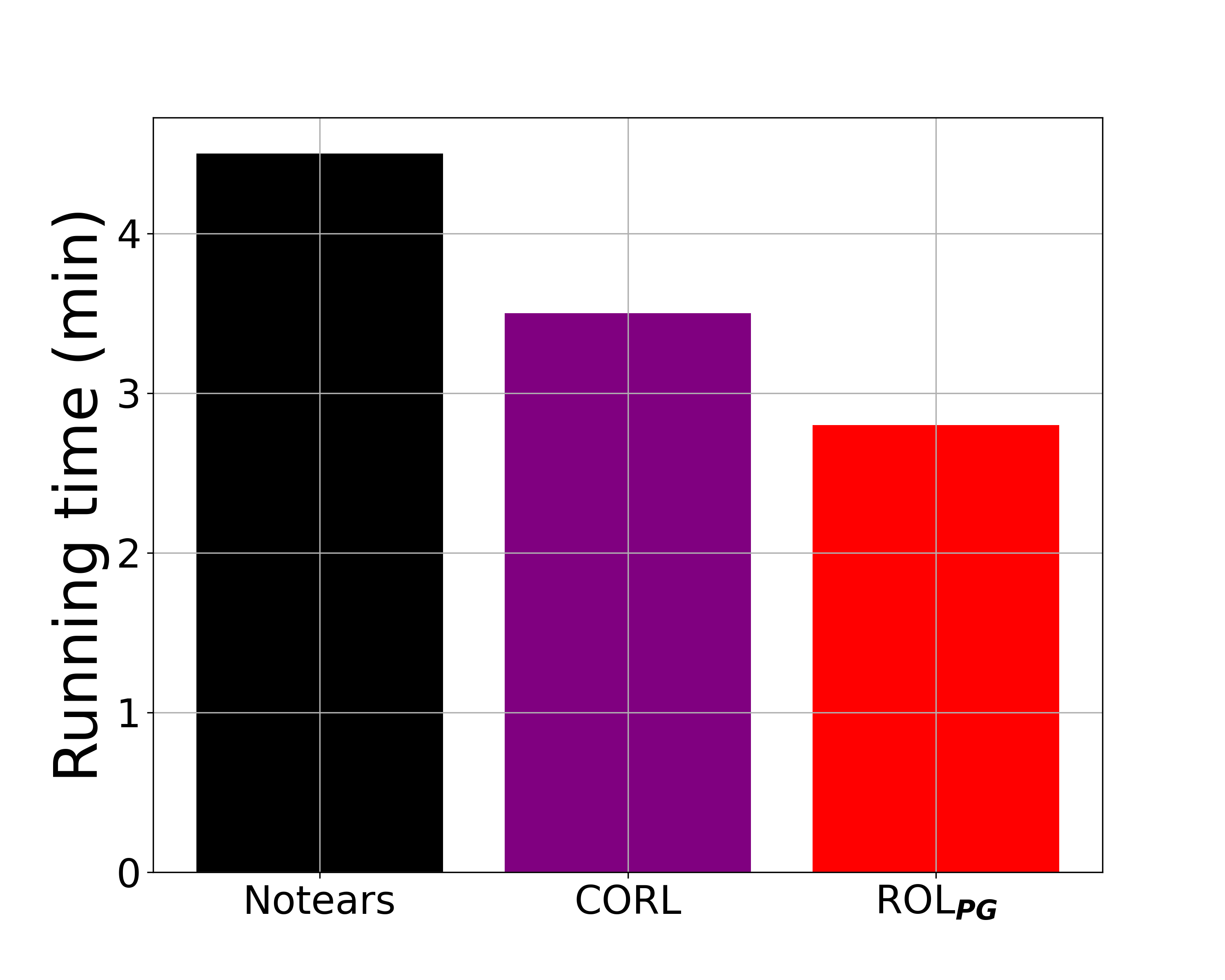
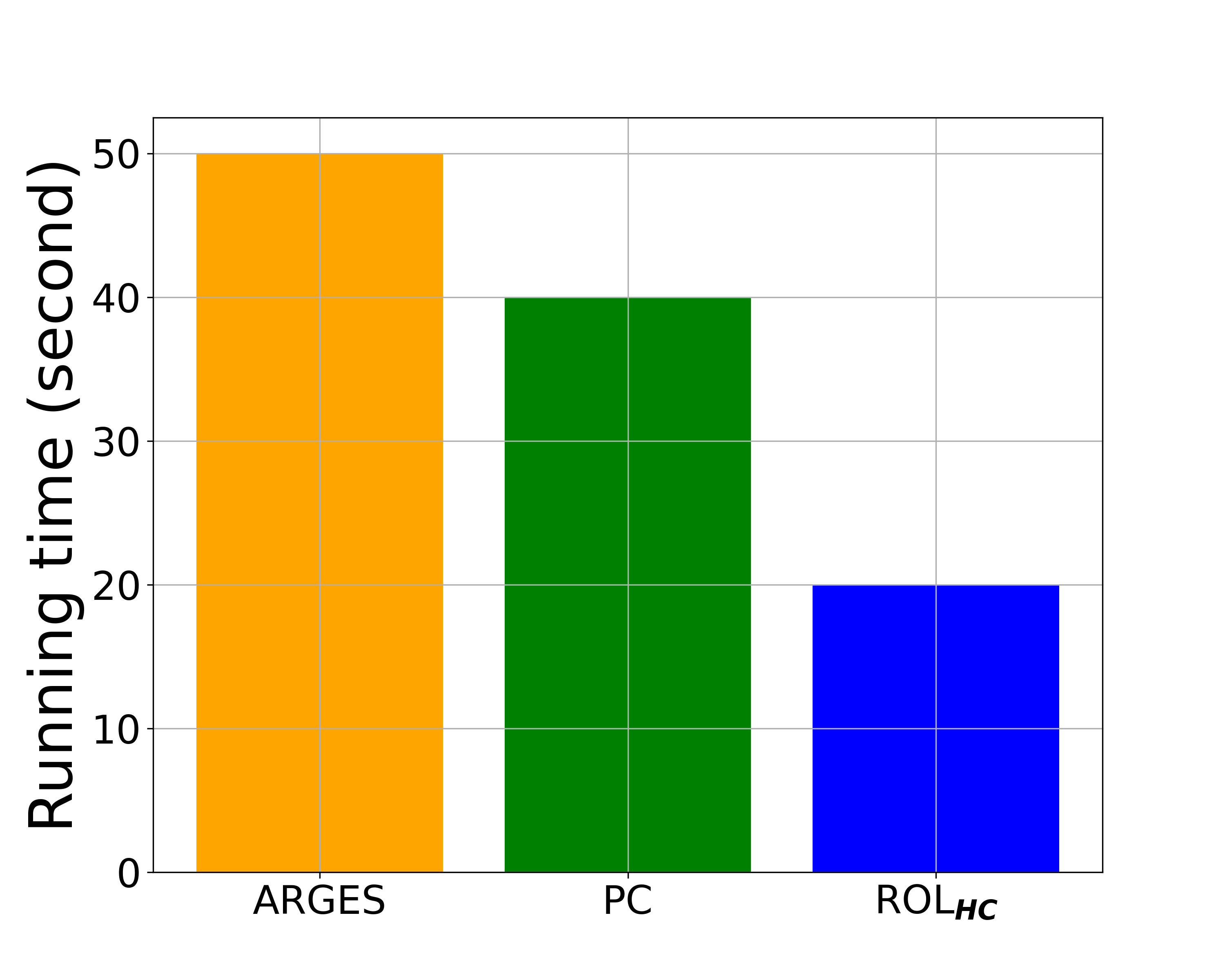
Figure 6: Runtime of various algorithms for learning graph Barley.

In general, ROL${}_{\text{HC}}$ is more scalable than RL-based algorithms. For example, ROL${}_{\text{HC}}$ could easily be applied on graphs with less than 200 variables with the computational power of a standard PC. ROL${}_{\text{VI}}$ which uses value-iteration, is limited to small size graphs with at most 35-40 variables. This can be improved by using approximation RL algorithms such as vanilla policy gradient. Our ROL${}_{\text{PG}}$ uses vanilla policy gradient.

In terms of the complexity of our algorithms, herein, we discuss the number of CI tests required by our algorithm. As we described in Appendix C.2, we used an algorithm for FindNeighbors that requires $|Mb(X)|$ number of CI tests. Hence, Algorithm 3 requires at most $(b-a)\alpha$ CI tests, where $\alpha$ is the size of the largest Markov boundary. Then, each iteration of Algorithm 3 (the implementation of ROL${}_{\text{HC}}$) performs at most $\mathcal{O}(n\ \text{maxSwap}^{2}\alpha)$ CI tests. Hence, ROL${}_{\text{HC}}$ performs at most $O(n\ \textit{maxIter}\ \textit{maxSwap}^{2}\alpha)$ CI tests.

C.5  Real-world Structures

In Table 3, we present more details about the real-world structures used in our experiments. In this table, $n$, $e$, $\Delta_{\text{in}}$, and $\Delta$ denote the number of vertices, number of edges, maximum in-degree, and maximum degree of the structures, respectively.

	Graph name	$n$	$e$	$\Delta_{\text{in}}$	$\Delta$
	Asia	8	8	2	4
	Sachs	11	17	3	7
	Insurance	27	51	3	9
	Water	32	66	5	8
	Alarm	37	46	4	6
	Ecoli70	46	70	4	11
	Barley	48	84	4	8
	Hailfinder	56	66	4	17
	Carpo	61	74	5	12
	Hepar2	70	123	6	19
	Arth150	107	150	6	20

Table 3: Detailed information of the real-world structures used in the experiments.

References

- Akbari et al. (2021) Akbari, S.; Mokhtarian, E.; Ghassami, A.; and Kiyavash, N. 2021. Recursive Causal Structure Learning in the Presence of Latent Variables and Selection Bias. Advances in Neural Information Processing Systems, 34.
- Alonso-Barba et al. (2013) Alonso-Barba, J. I.; Gámez, J. A.; Puerta, J. M.; et al. 2013. Scaling up the greedy equivalence search algorithm by constraining the search space of equivalence classes. International journal of approximate reasoning, 54(4): 429–451.
- Bernstein et al. (2020) Bernstein, D.; Saeed, B.; Squires, C.; and Uhler, C. 2020. Ordering-based causal structure learning in the presence of latent variables. In International Conference on Artificial Intelligence and Statistics, 4098–4108. PMLR.
- Bottou et al. (2013) Bottou, L.; Peters, J.; Quiñonero-Candela, J.; Charles, D. X.; Chickering, D. M.; Portugaly, E.; Ray, D.; Simard, P.; and Snelson, E. 2013. Counterfactual Reasoning and Learning Systems: The Example of Computational Advertising. Journal of Machine Learning Research, 14(11).
- Claassen, Mooij, and Heskes (2013) Claassen, T.; Mooij, J. M.; and Heskes, T. 2013. Learning Sparse Causal Models is not NP-hard. In In Proceedings of the 29th Annual Conference on Uncertainty in Artificial Intelligence (UAI), 172–181.
- Colombo et al. (2012) Colombo, D.; Maathuis, M. H.; Kalisch, M.; and Richardson, T. S. 2012. Learning high-dimensional directed acyclic graphs with latent and selection variables. The Annals of Statistics, 294–321.
- Erdős and Rényi (1960) Erdős, P.; and Rényi, A. 1960. On the evolution of random graphs. Publications of the Mathematical Institute of the Hungarian Academy of Sciences, 5: 17–61.
- Friedman and Koller (2003) Friedman, N.; and Koller, D. 2003. Being Bayesian about network structure. A Bayesian approach to structure discovery in Bayesian networks. Machine learning, 50(1): 95–125.
- Gámez, Mateo, and Puerta (2011) Gámez, J. A.; Mateo, J. L.; and Puerta, J. M. 2011. Learning Bayesian networks by hill climbing: efficient methods based on progressive restriction of the neighborhood. Data Mining and Knowledge Discovery, 22(1): 106–148.
- garage contributors (2019) garage contributors, T. 2019. Garage: A toolkit for reproducible reinforcement learning research. https://github.com/rlworkgroup/garage.
- Lachapelle et al. (2020) Lachapelle, S.; Brouillard, P.; Deleu, T.; and Lacoste-Julien, S. 2020. Gradient-based neural dag learning. ICLR.
- Larranaga et al. (1996) Larranaga, P.; Kuijpers, C. M.; Murga, R. H.; and Yurramendi, Y. 1996. Learning Bayesian network structures by searching for the best ordering with genetic algorithms. IEEE transactions on systems, man, and cybernetics-part A: systems and humans, 26(4): 487–493.
- Margaritis and Thrun (1999) Margaritis, D.; and Thrun, S. 1999. Bayesian network induction via local neighborhoods. Advances in Neural Information Processing Systems, 12: 505–511.
- Mnih et al. (2013) Mnih, V.; Kavukcuoglu, K.; Silver, D.; Graves, A.; Antonoglou, I.; Wierstra, D.; and Riedmiller, M. 2013. Playing atari with deep reinforcement learning. arXiv preprint arXiv:1312.5602.
- Mokhtarian et al. (2021) Mokhtarian, E.; Akbari, S.; Ghassami, A.; and Kiyavash, N. 2021. A recursive Markov boundary-based approach to causal structure learning. In The KDD’21 Workshop on Causal Discovery, 26–54. PMLR.
- Mokhtarian et al. (2022) Mokhtarian, E.; Akbari, S.; Jamshidi, F.; Etesami, J.; and Kiyavash, N. 2022. Learning Bayesian networks in the presence of structural side information. Proceeding of AAAI-22, the Thirty-Sixth AAAI Conference on Artificial Intelligence.
- Nandy, Hauser, and Maathuis (2018) Nandy, P.; Hauser, A.; and Maathuis, M. H. 2018. High-dimensional consistency in score-based and hybrid structure learning. The Annals of Statistics, 46(6A): 3151–3183.
- Ng et al. (2022) Ng, I.; Zhu, S.; Fang, Z.; Li, H.; Chen, Z.; and Wang, J. 2022. Masked gradient-based causal structure learning. In Proceedings of the 2022 SIAM International Conference on Data Mining (SDM), 424–432. SIAM.
- Pearl (2009) Pearl, J. 2009. Causality. Cambridge university press.
- Pellet and Elisseeff (2008a) Pellet, J.-P.; and Elisseeff, A. 2008a. Finding latent causes in causal networks: an efficient approach based on Markov blankets. Neural Information Processing Systems Foundation.
- Pellet and Elisseeff (2008b) Pellet, J.-P.; and Elisseeff, A. 2008b. Using Markov blankets for causal structure learning. Journal of Machine Learning Research, 9(Jul): 1295–1342.
- Rahman et al. (2021) Rahman, M. M.; Rasheed, A.; Khan, M. M.; Javidian, M. A.; Jamshidi, P.; and Mamun-Or-Rashid, M. 2021. Accelerating Recursive Partition-Based Causal Structure Learning. In Proceedings of the 20th International Conference on Autonomous Agents and MultiAgent Systems, 1028–1036.
- Raskutti and Uhler (2018) Raskutti, G.; and Uhler, C. 2018. Learning directed acyclic graph models based on sparsest permutations. ISI Journal for the Rapid Dissemination of Statistics Research.
- Russo (2010) Russo, F. 2010. Causality and causal modelling in the social sciences. Springer Dordrecht.
- Sachs et al. (2005) Sachs, K.; Perez, O.; Pe’er, D.; Lauffenburger, D. A.; and Nolan, G. P. 2005. Causal protein-signaling networks derived from multiparameter single-cell data. Science, 308(5721): 523–529.
- Schmidt et al. (2007) Schmidt, M.; Niculescu-Mizil, A.; Murphy, K.; et al. 2007. Learning graphical model structure using L1-regularization paths. In AAAI, volume 7, 1278–1283.
- Schulte et al. (2010) Schulte, O.; Frigo, G.; Greiner, R.; and Khosravi, H. 2010. The IMAP hybrid method for learning Gaussian Bayes nets. In Canadian Conference on Artificial Intelligence, 123–134. Springer.
- Spirtes et al. (2000) Spirtes, P.; Glymour, C. N.; Scheines, R.; and Heckerman, D. 2000. Causation, prediction, and search. MIT press.
- Sun et al. (2007) Sun, X.; Janzing, D.; Schölkopf, B.; and Fukumizu, K. 2007. A kernel-based causal learning algorithm. In Proceedings of the 24th international conference on Machine learning, 855–862.
- Sutton and Barto (2018) Sutton, R. S.; and Barto, A. G. 2018. Reinforcement learning: An introduction. MIT press.
- Sutton et al. (1999) Sutton, R. S.; McAllester, D.; Singh, S.; and Mansour, Y. 1999. Policy gradient methods for reinforcement learning with function approximation. Advances in neural information processing systems, 12.
- Teyssier and Koller (2005) Teyssier, M.; and Koller, D. 2005. Ordering-based search: A simple and effective algorithm for learning Bayesian networks. In Proceedings of the 21st Annual Conference on Uncertainty in Artificial Intelligence (UAI), 584–590.
- Tsamardinos, Aliferis, and Statnikov (2003) Tsamardinos, I.; Aliferis, C. F.; and Statnikov, A. 2003. Time and sample efficient discovery of Markov blankets and direct causal relations. In Proceedings of the ninth ACM SIGKDD international conference on Knowledge discovery and data mining, 673–678.
- Tsamardinos, Brown, and Aliferis (2006) Tsamardinos, I.; Brown, L. E.; and Aliferis, C. F. 2006. The max-min hill-climbing Bayesian network structure learning algorithm. Machine learning, 65(1): 31–78.
- Tsirlis et al. (2018) Tsirlis, K.; Lagani, V.; Triantafillou, S.; and Tsamardinos, I. 2018. On scoring maximal ancestral graphs with the max–min hill climbing algorithm. International Journal of Approximate Reasoning, 102: 74–85.
- Verma and Pearl (1991) Verma, T.; and Pearl, J. 1991. Equivalence and synthesis of causal models. UCLA, Computer Science Department.
- Wang et al. (2021) Wang, X.; Du, Y.; Zhu, S.; Ke, L.; Chen, Z.; Hao, J.; and Wang, J. 2021. Ordering-based causal discovery with reinforcement learning. International Joint Conference on Artificial Intelligence (IJCAI).
- Watkins and Dayan (1992) Watkins, C. J.; and Dayan, P. 1992. Q-learning. Machine learning, 8(3): 279–292.
- Williams (1992) Williams, R. J. 1992. Simple statistical gradient-following algorithms for connectionist reinforcement learning. Machine learning, 8(3): 229–256.
- Yu et al. (2019) Yu, Y.; Chen, J.; Gao, T.; and Yu, M. 2019. DAG-GNN: DAG structure learning with graph neural networks. In International Conference on Machine Learning, 7154–7163. PMLR.
- Zhang et al. (2019) Zhang, H.; Zhou, S.; Yan, C.; Guan, J.; and Wang, X. 2019. Recursively learning causal structures using regression-based conditional independence test. In Proceedings of the AAAI Conference on Artificial Intelligence, volume 33, 3108–3115.
- Zhang (2008) Zhang, J. 2008. Causal reasoning with ancestral graphs. Journal of Machine Learning Research, 9: 1437–1474.
- Zhang et al. (2011) Zhang, K.; Peters, J.; Janzing, D.; and Schölkopf, B. 2011. Kernel-based conditional independence test and application in causal discovery. In Proceedings of the 27th Annual Conference on Uncertainty in Artificial Intelligence (UAI), 804–813.
- Zhang et al. (2017) Zhang, K.; Schölkopf, B.; Spirtes, P.; and Glymour, C. 2017. Learning causality and causality-related learning: Some recent progress. National Science Review, 5(1): 26–29.
- Zheng et al. (2018) Zheng, X.; Aragam, B.; Ravikumar, P. K.; and Xing, E. P. 2018. Dags with no tears: Continuous optimization for structure learning. Advances in Neural Information Processing Systems, 31.
- Zheng et al. (2020) Zheng, X.; Dan, C.; Aragam, B.; Ravikumar, P.; and Xing, E. 2020. Learning sparse nonparametric dags. In International Conference on Artificial Intelligence and Statistics, 3414–3425. PMLR.
- Zhu, Ng, and Chen (2020) Zhu, S.; Ng, I.; and Chen, Z. 2020. Causal discovery with reinforcement learning. ICLR.