Do Investors Hedge Against Green Swans?
Option-Implied Risk Aversion to Wildfires

Abstract

Measuring beliefs about natural disasters is challenging. Deep out-of-the-money options allow investors to hedge at a range of strikes and time horizons, thus the 3-dimensional surface of firm-level option prices provides information on (i) skewed and fat-tailed beliefs about the impact of natural disaster risk across space and time dimensions at daily frequency; and (ii) information on the covariance of wildfire-exposed stocks with investors’ marginal utility of wealth. Each publicly-traded company’s daily surface of option prices is matched with its network of establishments and wildfire perimeters over two decades. First, wildfires affect investors’ risk neutral probabilities at short and long maturities; investors price asymmetric downward tail risk and a probability of upward jumps. The volatility smile is more pronounced. Second, comparing risk-neutral and physical distributions reveals the option-implied risk aversion with respect to wildfire-exposed stock prices. Investors’ marginal utility of wealth is correlated with wildfire shocks. Option-implied risk aversion identifies the wildfire-exposed share of portfolios. For risk aversions consistent with Barro (2012), equity options suggest (i) investors hold larger shares of wildfire-exposed stocks than the market portfolio; or (ii) investors may have more pessimistic beliefs about wildfires’ impacts than what observed returns suggest, such as pricing low-probability unrealized downward tail risk. We calibrate options with models featuring both upward and downward risk. Results are consistent a significant pricing of downward jumps.

1 Introduction

Natural disaster risk is receiving increasing attention by both academics and policymakers preparing for a potential “Green Swan” [bolton2020green, rudebusch2021climate]. What are market participants’ beliefs about the wealth impact of natural disasters? Measuring such beliefs is challenging as they may be (a) asymmetric, as firms may lose or gain; (b) fat-tailed, as natural disasters may cause large jumps and volatility shifts; (c) non-stationary, as agents learn about the probability distribution of disaster risk over time; (d) heterogeneous, as firms have different levels of adaptation to disasters; and (e) ambiguous as different forecasters provide different probability distributions. A seminal literature uses surveys to measure beliefs about assets’ risk exposure [bakkensen2017flood], and about the evolution of future disaster risk [leiserowitz2010climate, ballew2019climate]. Yet, eliciting high frequency and spatially heterogeneous beliefs about climate risk for the United States at both local and national levels, and for short- and long-run time horizons, remains challenging.

The exchange-traded market for options is a fast-growing global market with a total volume of 33.3 billion contracts in 2021 that allows financial agents to trade hedges for firm-, time-, and maturity-specific risks. The surface of option prices by maturity and strike depends on market participants’ subjective probability distribution as well as the marginal utility of consumption or wealth, thus revealing the set of Arrow-Debreu prices for each level of each climate-exposed stock [breeden1978prices, ait2003nonparametric, beber2006effect, figlewski2018risk]. Such surface typically displays a ’smile’ or ’smirk’ that steepened significantly after the 1987 market crash [benzoni2011explaining], as market participants hedge against large downward and upward tail risks. Teasing out what, in Arrow Debreu state prices, is driven by the marginal utility of wealth and by beliefs about risks enables an estimation of investors’ aversion to natural disaster risks.

This paper measures the response of investors’ hedging to natural disaster shocks, compares this response to observed returns, and identifies investors’ option-implied risk aversion with respect to such natural disasters. It matches the universe of establishments, sales, and employment of publicly-traded firms between 2000 and 2018 to their daily surface of option prices by strike and maturity, and to the boundaries of wildfire perimeters reported by fire departments across the United States. First, the paper estimates the daily risk neutral distribution implied by the surface of option prices for all day-firms affected by a wildfire, and for an equal-sized set of control surfaces, at short-, medium-, and long-run time horizons. This panel approach can non-parametrically estimate the impact of wildfires on the risk neutral distribution over and above day- and firm-specific confounders. Second, over the last two decades the paper estimates a significant impact of exposure to wildfires on the price in deep out-of-the-money options, controlling for day- and firm-specific confounders. This increase in prices is over and above what a log normal distribution of stock prices would imply. Third, the paper compares such risk neutral probabilities to the physical probabilities, thus inferring investors’ marginal utility for each level of a wildfire-exposed stock. This yields a risk aversion parameter with respect to each wildfire-exposed stock. Fourth, the paper develops a continuous time merton1969lifetime model with a wildfire stock and the index to tease out risk aversion with respect to the index from that with respect to the wildfire-exposed stock. Portfolio shares are typically unobserved, and this paper’s novel approach provides, ‘in reverse’, the weight of wildfire stocks implied by deep out-of-the-money option prices. Fifth, the paper calibrates investors’ marginal utility at the levels of each wildfire-exposed stock to disentangle what, in the impact of wildfires on the risk neutral distribution is due to marginal utility from what is due to change in beliefs.

The paper puts forward and implements a fast and efficient way to identify the impact of natural disasters on investors’ risk-neutral probability distributions for each firm and for each maturity at daily frequency. Using such daily probability surfaces, the paper estimates the impact of wildfires on the risk neutral distribution non-parametrically when affected by a wildfire. This enables an estimation of the impact of wildfires on beliefs’ (a) asymmetry, (b) fat tails, and (c) non-stationarity. Results suggest that when a firm’s network of establishments is exposed to a wildfire, the risk neutral probability of downward tail events increases but is heterogeneous across industries, while they have a small but precisely estimated positive impact on the risk neutral probability of upward movements. Impacts are observed for short and long maturities.

Backing out risk neutral distributions from option prices requires using arbitrage-free prices. Since such arbitrage opportunities may be observed, prices are converted into arbitrage-free prices that do not exhibit possibilities of butterfly, calendar spread, or call spread arbitrage [carr2005note]. Yet, wildfires show little correlation with the difference between arbitrage-free and observed prices, suggesting that there may be few opportunities to take advantage of ‘climate risk’ arbitrage opportunities in vanilla option markets. This also suggests that arbitrage opportunities are unlikely to drive the paper’s main findings.

Investors’ hedging against downward and upward tail risks is typically associated with a steeper implied volatility smile [bakshi2003stock]. The surface of implied volatilities is a simple transformation of the surface of option prices such that, if the firm’s stock followed a geometric diffusion process, the implied volatility would be independent of strike and maturity. In the short-run, wildfires have a greater impact on the implied volatility smile for low strikes than for strikes higher than the forward price: the impact is asymmetric, suggesting that market participants hedge more against the downside than for the upside. Over medium and long run time horizons, the lower hedging for the upside remains: markets price a lower probability of an upside. Impacts are long-lasting, with a smile that persists after the first wildfire.

Results on the risk neutral distribution and the volatility smile are obtained either in a linear panel data regression with day and firm fixed effects with daily data between 2000 and 2018; they are also obtained using a more flexible non-parametric approach pooling all day-firm surfaces after orthogonalization with respect to firm and day-specific confounders.

Option prices can also enable an identification of the correlation of investor’s wealth with wildfires. Arrow Debreu state prices are the product of the marginal utility of investors, the physical probability of each state, and the risk free discount factor. As each wildfire-exposed stock represents a small share of the S&P 500, wildfire stocks could be statistically uncorrelated with investors’ wealth, once controlling for the stock’s beta with respect to the index. If movements in wildfire-exposed stocks were uncorrelated with investors’ marginal utility of wealth or consumption, risk neutral probabilities would be proportional to the physical probabilities. We compare the Arrow Debreu state prices for each day-firm to the physical probability distribution of future returns to estimate investors’ risk aversion with respect to the wildfire stocks. This also identifies the marginal utility of investors at each level of the wildfire-exposed stock. The first finding is that the ratio of risk neutral to physical probabilities significantly differs from a constant for treated stocks. This suggests that investors’ marginal utility is significantly correlated with wildfire shocks. Results provide a firm-level elasticity of state prices with respect to the level of the stock.

Such risk aversion with respect to a specific stock can reveal the weight of the stock in the investor’s portfolio. We develop a merton1971optimum portfolio allocation problem with two risky assets, the index and a wildfire-exposed stock, to separately identify what, in investors’ demand for equity options, is driven by the beta of the wildfire-exposed stock w.r.t the index from what is driven by wildfires. Proposition 1 of Section 5.1 shows that the Arrow-Pratt risk aversion with respect to a single stock is proportional to the relative risk aversion with respect to wealth, where the proportionality constant is a linear function of the share of the stock in the investor’s portfolio and the beta of the stock w.r.t. the market. Using the option-implied risk aversion with respect to the stock, assuming that the investor holds the market portfolio, and using the estimated betas from CRSP, we can identify the risk aversion with respect to wealth that is consistent with the option-implied risk aversion with respect to the wildfire-exposed stock.

Assuming the market portfolio, the option-implied relative risk aversion w.r.t wealth is significantly higher than that suggested by barro2006rare, barro2012rare, or mehra1985equity. This is consistent with (i) investors holding shares of wildfire-exposed stocks larger than what the market portfolio implies, markets may be segmented as in gabaix2007limits; (ii) a mismeasurement of the physical probability distribution, which reflects investors’ beliefs; thus investors’ beliefs are not well captured by the realization of past or future returns; this would include investors’ expectations of rare tail risk, that does not materialize with high enough frequency in the sample of wildfire-exposed stocks, a phenomenon suggested for the index by barro2012rare.

The last part of the paper parameterizes the risk neutral distribution using merton1976option jump-diffusion model, and kou2004option double exponential jump model to be able to observe the pricing of both upward and downward shocks in the same model. Results of this calibration on the treatment group (affected by wildfires) and the control group (unaffected) suggest a small increase in the pricing of upward jumps, but a doubling in the risk-neutral magnitude of downward jumps.

merton1976option suggests that jumps are a source of market incompleteness, as riskless delta hedging is not typically feasible. A set of state-contingent parametric insurance, with a payoff tied to the occurrence of wildfires for each specific area, could allow market participants to hedge wildfire risk. The calibration of the options, by providing the risk neutral distribution, allows the pricing of such parametric insurance.

This paper contributes to at least three literatures. First, the growing literature on the impact of natural disaster on option prices. kruttli2021pricing important contribution provides convincing evidence of an increase in the at-the-money implied volatility of firms affected by a hurricane. The paper also finds that, for firms hit by hurricanes, the variance risk premium, i.e. the difference between the implied volatility and the realized volatility, is a significant predictor of future stock returns. This paper’s model-free approach to the recovery of the risk neutral distribution from option prices has two benefits that complement kruttli2021pricing key insights. First, this paper provides the entire probability distribution by stock level and by time horizon (maturity) and thus can separate symmetric uncertainty (volatility) from asymmetric expectations of gains and losses. As such, this paper’s approach reveals the response of the moments of the risk neutral distribution and the downside and upside hedging of investors: this enables an identification of downward and upward tail risks separately, as investors perceive the possibility of firms’ recovery in the short-, medium-, and long-run. This enables the identification of jump risk separately from stochastic volatility, as the calibration of option prices as in duffie2000transform enables the identification of the jump diffusion processes consistent with the surface of option prices. An emerging literature studies the skewness risk premium [orlowski2020nature]. Second, this paper’s approach has the benefit of identifying investors’ option-implied risk aversion, and thus reveals the importance of wildfire shocks for investors’ portfolio. Results suggest that wildfire shocks matter more than if investors held the market portfolio.

This paper also contributes to the literature on the estimation of beliefs. An important literature uses surveys to measure beliefs about the specific risk exposure of assets [bakkensen2017flood], and about the evolution of future climate risk [leiserowitz2010climate, ballew2019climate]. The economics literature has shown that stated beliefs have predictive power for individual behavior [manski2018survey], predict portfolio allocation [giglio2021five] and shape macroeconomic outcomes [fuster2010natural]. This paper suggests that option prices provide a low-cost, high-frequency, and spatially heterogeneous way of measuring beliefs in natural disaster risk at multiple time horizons. The absence of a significant correlation between arbitrage opportunities and wildfire risk suggests that this recovers well-behaved impacts on the risk neutral probability distribution.

This paper contributes to the literature on risk aversion and asset pricing. In the mortgage-backed securities (MBS) market, gabaix2007limits suggests that prepayment risk, which is diversified in the aggregate, is priced in MBS yields. They also find that the sign for the correlation between income and yields is the opposite of what would be expected. Their conclusion is that markets are segmented. This paper is also in the flavor of froot1999pricing, which finds that the price of catastrophe reinsurance is unusually high, lending support for a segmented trading of such assets; in this paper, we find that the pricing of deep out of the money puts is significantly higher than the pricing when investors hold a diversified portfolio.

The response of option prices to transitory shocks is akin to dessaint2017managers finding that the managers of firms located next to hurricane-hit areas tend to express concerns about hurricanes in their 10-Ks/10-Qs, and increase cash holdings, even when actual risk remains unchanged. This paper suggests that such concerns translate into the pricing of downward tail risk in out-of-the-money options, but also in upward tail risk pricing. It is also closely related to orlik2014understanding on Black Swans: when people form expectations like Bayesian econometricians, and when they estimate tail risk probabilities dynamically, small changes in estimated skewness cause large changes that “whip around” the probabilities of unobserved tail events.

Finally, this paper contributes to the literature on firms’ adaptation to natural disaster risk [kahn2020climate]. This paper provides a method for identifying the option-implied price of wildfire insurance, a set of state-contingent and spatially-located Arrow Debreu assets whose price is the risk neutral price of downward tail risk. This paper’s wildfire data suggests a significant upward trend in the probability that a Zip code is in a wildfire perimeter. Results suggest long-run impacts of wildfires on the implied volatility smile, but such long-run impacts are priced in after the first exposure to a wildfire rather than cumulatively per wildfire. Hence option prices may provide an adaptation signal [kahn2021adapting]. Out of the money put and call options are part of the set of hedging devices that enable investors to weather natural disaster risks. And, in reverse, investors’ demand for such options reveals their expectations of firms’ ability to adapt to natural disasters. In this sense, this paper’s causal estimates are the reduced-form estimates of firms’ adaptation responses.

The paper is structured as follows. Section 2 describes the main data set: the daily set of option implied volatilities and prices by strike and maturity, matched to each publicly-traded firm’s geocoded network of establishments and wildfire perimeters. Section 3 describes the relationship between option prices and their implied risk neutral distribution. It estimates the firm-level risk neutral distribution at daily frequency between 2000 and 2018 for listed firms using the convexity of option prices. It estimates the impact of wildfires on the risk neutral moments, the lower and upper tails, as well as the central part of the probability distribution. Section 4 estimates the model-free impact of wildfires on the volatility smile, using daily longitudinal panel data controlling for day and firm-level unobservables. Section 5 then estimates the relationship between the risk neutral distribution and the physical distribution for wildfire-exposed stocks, thus identifying a correlation between investors’ marginal utility and the value of wildfire-exposed stocks. This yields an option-implied risk aversion. Section 7 calibrates the surface of option prices to tease out whether wildfires cause in upward and downward jump intensity or magnitude. Section 8 concludes.

2 Data Sets

Estimating the impact of natural disasters on the surface of option prices, on Arrow-Debreu prices, and on investors’ beliefs requires four data sets. First, the universe of establishments of publicly-traded companies. Second, the spatial footprint of natural disasters at daily frequency. Third, option prices by maturity and strike at daily frequency. Fourth, stock prices and dividends to build physical probability distributions that can be compared to the risk-neutral distribution of Arrow-Debreu prices.

2.1 The Geography of Publicly-Traded Companies’ Establishments

The first source of data is Dun and Bradstreet’s NETS for the 50 states and the District of Columbia between 2000 and 2018. NETS provides the geographic location of establishments, with their employment, sales, and 8-digit NAICS code at annual frequency. barnatchez2017assessment compares NETS data to the County Business Patterns (CBP), the Nonemployer Statistics, and the Quarterly Census of Employment and Wages (QCEW) and finds that the data set covers three quarters of U.S. private sector employment. The study finds that the county-level correlation of NETS employment and CBP employment is typically above 0.99. We follow the convention of echeverri2019chasing in omitting the last two years of data, which can be subject to revisions. Other studies using NETS and comparing it to administrative data counts include neumark2011small. Recent work using NETS includes song2019firming.

A key feature of NETS is its inclusion of the ticker symbol when the establishment is the headquarters of a publicly-traded firm. It also links a parent firm with its subsidiaries. Hence the data enable the estimation of each publicly-traded firm’s geographic footprint. We compute the number of establishments, the employment, and the sales of each publicly traded firm in each 5-digit Zip code. As NETS is longitudinal, the data also enable the estimation of the relocation of a firm’s establishments over time in response to climate shocks. Thus this paper’s estimates use the firm’s latest measured geographic footprint and exposure to wildfires, which may respond to expectations or experiences of climate risk.

2.2 Wildfire Risk

Wildfire perimeters and dates are provided by the Development and Application team of Wildland Fire Management Research at the National Interagency Fire Center. Such center coordinates the actions of local firefighting agencies and records the polygon of each fire’s perimeter, the date of the fire, the number of acres burnt, the reporting agency; for a total of 43,114 wildfire perimeters on 829 separate dates, with an average of 726 perimeters per year, 67 million acres in total, and an average of 3,771 acres per perimeter. For each 5-digit Zip Code (Census ZCTAs) we record the area of the Zip code intersecting the wildfire perimeter in the US National Atlas Equal Area coordinate reference system. Wildfires affected 1,964 5-digit Zip codes. The share of a publicly-traded firm’s establishments, sales, and employment hit by a wildfire depends on the share of its establishments in each of the US’s 33,120 ZCTAs. We use the boundaries of 2014 ZCTAs. The log number of establishments, employees, and sales hit by a wildfire according to this definition are presented on Appendix Figure A. The figures suggest a substantial increase in the number of establishments, employees, and sales hit by a wildfire over time.

2.3 Option Prices and Implied Volatility

Our option data comes from OptionMetrics’ IvyDB US, which covers all US-listed equity options. We consider data on the same time period as the Dun and Bradstreet data, i.e. from January 2000 till December 2018. The data include the strike, maturity, call/put indicator, best bid/ask prices and we use the midpoint as the option price. We estimate the moneyness of the option using ratio of the strike over the forward price. Implied volatility is obtained by OptionMetrics using binomial trees, which account for the possibility of early exercise. Option prices are de-Americanized using the methodology described by burkovska2018calibration, which converts binomial-tree implied volatilities into European option prices. In total, this comprises 2.36 billion equity option $\times$ day $\times$ maturity $\times$ strike observations. To work with a more manageable data set amenable to a panel regression with multi-way fixed effects, we (i) include all option prices of treated (wildfire-exposed) firms, and (ii) a random sample of 500 untreated firms on a random 5% of trading days. We end up with a sample of 16,842,463 option prices.

2.4 Descriptive Statistics

Figure 1(a) presents the spatial distribution of publicly-listed companies’ employment. For each listed company, the map estimates the number of employees in each 5-digit Zip code on average between 2000 and 2018, represented by colors from black to yellow. The black dots are for the headquarters. The map suggests that NETS data covers the coterminous United States, and that the employment captured in this paper extends beyond the location of the headquarters. Figure 1(b) presents the spatial distribution of wildfires between 2000 and 2018. The colors correspond to the number of years that a 5-digit Zip code was hit by a wildfire. The map suggests that wildfires hit most of the forests of the Western part of the United States, forests of the Pacific Northwest and Southwest, the Intermountain area, the Northern region, the Rocky Mountain region, and the Southwestern region. They also affected the George Washington and Jefferson forests in the Appalachians, the Ozark and Ouachita forests in Arkansas, Southernwestern Florida, but also the Sam Houston forest in Texas, the Tallageda forest in Alabama.

3 Option-Implied Risk Neutral Probabilities of Natural Disasters

3.1 Identifying Probability Distributions from the Surface of Option Prices

The surface of option prices by maturity and by strike reveals market participants’ set of Arrow Debreu prices at each level of the future stock price and for each maturity. This appears when considering the price of a European option, which can be exercised at maturity, before considering the case of American options. At time $t$, the payoff of a European call option with maturity $T$ and with strike $K$ is the expectation of the payoff at $T$:

$$C(K,T,t)=e^{-r(T-t)}\mathbb{E}_{t}^{\mathbb{Q}}\left[\max(S_{T}-K,0)\right],$$ (1)

where the expectation is taken at $t$ with respect to the risk neutral distribution, whose pdf is denoted $f^{*}(S_{T})$, consistent with the notations of ait1998nonparametric. This risk neutral distribution $f^{*}$ typically differs from the physical distribution of the stock price, noted $f$. We investigate what we learn from their differences in Section 5.1. The price of the option is thus:

$$C(K,T,t)=e^{-r(T-t)}\int_{K}^{\infty}(s-K)f^{*}(s)ds,$$ (2)

where $r$ is the risk-free rate.

When the strike $K$ increases marginally, it has two impacts on the call price. First, the lower bound of integration changes, and second the payoff $S_{T}-K$ declines. breeden1978prices shows that this leads to a simple relationship between the derivatives of the option price with respect to the strike and the risk neutral distribution:

$$\left.\frac{\partial^{2}C}{\partial K^{2}}\right|_{K=S_{T}}=e^{-r(T-t)}f^{*}(S_{T}),\qquad\textrm{and}\qquad\left.\frac{\partial C}{\partial K}\right|_{K=S_{T}}=-e^{-r(T-t)}\left[1-F^{*}(S_{T})\right],$$ (3)

where $F^{*}$ is the cumulative risk neutral distribution function. Hence this suggests that the convexity of option prices at the strike $K=S_{T}$ identifies the price of an Arrow-Debreu asset that pays off $1 when $S=S_{T}$ at maturity $T$. This key result, implemented using arbitrage-free approaches of ait2003nonparametric enables an estimation of the Arrow-Debreu prices of states in which a climate shock hits.

This approach provides the risk neutral distribution at each time $t$, for each stock price $S_{T}$, and for each maturity $T$. It enables an estimation that depends on investors’ time horizon, an estimation of belief updating, and recovers a rich probability distribution parameterized by exposure to wildfires, allowing a comparison $f^{*}(S_{t}|\text{Disaster}=1)-f^{*}(S_{t}|\text{Disaster}=0)=\Delta f^{*}(S_{t})$ at each future level of the stock for a range of maturities.

3.2 Estimation Technique: Arbitrage Free Prices and the Convexity of Option Prices

breeden1978prices approach described in equation (3) suggests that the convexity of option prices reveals the risk neutral distribution for each maturity. Practical implementation requires arbitrage-free option prices.

Observed option prices may display arbitrage opportunities [carr2005note], and a naive approach consisting of taking the second-difference of observed prices may not yield the risk neutral distribution. First, call prices may not be convex, which may be a source of butterfly arbitrage [carr2005note]. Second, call prices may not be decreasing in the strike, which may lead to a call spread arbitrage opportunity. Third, observed call prices may not be higher than $S-Ke^{-r(T-t)}$, leading to potential calendar spread arbitrage.

We address this concern by estimating arbitrage-free option prices using a method close to the approach of ait2003nonparametric. We first de-Americanize option prices using the method described in Section 2.3. We then estimate the closest prices, in the least-squares sense, that satisfy the three no-arbitrage conditions above. This is done by a constrained linear least squares similar to ait2003nonparametric but allowing here for an unequal grid of strikes whenever such grid is observed. Such unequal strike steps are common when considering options on individual equities. This first step yields a vector of arbitrage-free call prices for each observed strike.

Finally, we estimate the second derivative with a local polynomial regression of order 4 with a Gaussian kernel. The second-derivative of option prices is the coefficient of the second order term in the strike. In contrast with malz2014simple, we allow the probabilities to be nonzero at the boundaries of the support of traded strikes and assess the impact of wildfires on the support of traded strikes in a second step. Both steps (arbitrage free and second derivative) rely on a constrained least squares approach with an interior point optimization algorithm.We use a grid of 100 equally spaced strikes $K\in\left[\underline{K}_{jtT},\overline{K}_{jtT}\right]$, with the same range as the observed strikes $K_{jtTk}$ for $k=1,2,\dots,$. $\left[\underline{K}_{jtT},\overline{K}_{jtT}\right]$ is the support. Formally, the risk neutral distribution at point $K$ is the coefficient $\beta_{2}$ in the optimization program:

$$\min_{\beta_{p},p=0,\dots,4} \sum_{i=1}^{N}\left[C_{i}-\sum_{p=0}^{4}\beta_{p}(k_{i}-K)^{p}\right]K_{h}(k_{i}-K)$$ (4)

with $\beta_{2}\geq 0$. The function $K_{h}(x)=K(x/h)/h$ is a Gaussian kernel, where the bandwidth $h$ was selected as in ait2003nonparametric.

Important alternative methods include jackwerth1996recovering and figlewski2009estimating. Recent reviews include figlewski2018risk and cuesdeanu2018pricing.

3.3 Wildfires and Arbitrage Opportunities

To see whether wildfires cause the emergence or the increase in arbitrage opportunities, we compute the difference between the arbitrage-free prices of ait2003nonparametric and the observed prices. We regress such difference on the treatment indicator variable at different maturities. Results are presented on Appendix Table C, with three different approaches for the dependent variable. Column (1) uses the dollar difference, column (2) the absolute value of the dollar difference, and column (3) the log of the absolute value of the difference. The table presents results for 5 different ranges of maturities. Results are similar when pooling all maturities. Results suggest that most coefficients on the treatment indicator are not significant, and often of small magnitude. These results also suggest that there may not be ‘climate risk’ arbitrage opportunities based on the butterfly, the calendar, and call spreads.

3.4 PG&E’s Risk Neutral Distribution during the October 2017 Wildfires

The Northern California wildfires broke a record as the most destructive wildfires in California’s history, with an estimated 44 deaths, 250,000 acres hit [mass2019northern], 100,000 evacuated and 8,900 structures destroyed.. The California Department of Forestry and Fire Protection released a report on June 8, 2018 stating that:

After extensive and thorough investigations, CAL FIRE investigators have determined that 12 Northern California wildfires in the October 2017 Fire Siege were caused by electric power and distribution lines, conductors and the failure of power poles.

The PG&E Fire Victim Trust filed a lawsuit on February 24, 2021 arguing that ”The 2017 North Bay Fires Could Have Been Prevented If PG&E Had Implemented A De-Energization Program” and that ”PG&E Should Have Cut Off Power Because It Had Failed to Maintain Vegetation in Violation of Applicable Regulations.” While it took significant time for courts and CAL FIRE to describe their assessment of responsibilities, the evidence below suggests that option markets reacted quickly and provided investors with hedges against tail risk and rising, potentially stochastic, volatility.

Results are presented on Figure 2 for October 2, October 12, November 7 and November 30. The colors correspond to the traded maturities of the options. The maturity is in fraction of a year. The RND distribution suggests a clear asymmetry in investors’ risk neutral expectations. Hedges against tail risk appear as soon as October 2, and become more evident during the wildfire (figure (b)) and after the wildfire. In the aftermath of the wildfire, hedges for downside risk appear for both shorter-dated and for longer-dated options. The risk neutral distribution displays both negative skewness and negative kurtosis that become more pronounced over time.

3.5 Panel Data Impacts on the Risk Neutral Distribution: Identification Challenges

Estimating the causal impact of wildfires on listed firms’ out-of-the-money option prices, risk neutral probabilities, and implied volatility is challenging for at least four reasons. First, firms affected by wildfires may already have stock prices that are more likely to exhibit average skewness and kurtosis, asymmetric jumps and stochastic volatility, independently of wildfires. Second, wildfires may occur on days where the market is overall more likely to experience skewness and kurtosis in returns, jumps and stochastic volatility. Third, wildfires may coincide with other adverse or positive events for the firm. Fourth, option prices may exhibit arbitrage opportunities, including non-convexities.

The causal impact of wildfires on out-of-the-money option prices may also be heterogeneous across firms depending on their adaptation or expected ability to adapt to wildfire shocks. Firms that are expected to be resilient to wildfires may experience a smaller or no increase in the price of out-of-the-money puts. Firms that are expected to gain or be affected only shortly may experience increases in the price of out-of-the-money calls.

3.6 Panel Data Estimates: Wildfires and Arrow Debreu State Prices

We then turn to the estimation of the impact of wildfires on the risk neutral distribution or Arrow Debreu state prices. The approach described for PG&E is applied systematically to stocks of the treatment group, and, for computational reasons, to a random sample of the control group of the same size as the treatment group.

As in the previous sections, we wish to identify the causal impact of wildfires over and above the confounding impact of shocks specific to the day of wildfires and shocks specific to firms. The following regression estimates the impact of wildfires controlling for non-time-varying firm-level and day-specific confounders:

$$f_{j,t,T,m}^{*}=\sum_{\ell=1}^{M}\nu_{\ell}\mathbf{1}(m=\ell)+\mathbf{1}(\textrm{Treated}_{j,t})\sum_{\ell=1}^{M}\delta_{\ell}\mathbf{1}(m=\ell)+\textrm{Firm}\times\text{Moneyness}_{jm}+\textrm{Date}_{t}+\varepsilon_{j,t,T,k}$$ (5)

where $f_{j,t,T,m}^{*}$ is the risk neutral distribution obtained using the ait2003nonparametric approach for firm $j$ on day $t$ at maturity $T$ for moneyness levels on a grid of $M$ equally-spaced moneynesses on the observed support. $\mathbf{1}(\textrm{Treated}_{j,t})$ an indicator variable equal to 1 either when (a) firm $j$ is exposed to a wildfire on day $t$, (b) firm $j$ has been exposed to a wildfire any time before $t$, (c) firm $j$ has been exposed to its last recorded wildfire any time before $t$. $\delta_{\ell}$ is the set of coefficients of interest. $\nu_{\ell}$ captures the baseline distribution. Standard errors are double-clustered as in cameron2011robust at the firm and date levels.

This specification is flexible as it allows an estimation of the impact of wildfire on each part of the risk neutral distribution separately. It is also demanding in terms of inference and statistical power when the grid of moneyness levels $m=1,\dots,M$ is fine-grained.

Another approach is to estimate a treatment effect at each moneyness level, weighing observations depending on how far (in a kernel weighting sense) from the moneyness level of interest. We are interested in measuring the treatment effect for moneyness level $m\in\{1,2,\dots,M\}$:

$$\text{TE}_{m}=E(f_{j,t,T,m}^{*}|\text{Treated}_{j,t}=1)-E(f_{j,t,T,m}^{*}|\text{Treated}_{j,t}=0),$$ (6)

and each expectation can be approximated using local polynomial regression. This yields an estimator for the treatment effect based on a two-way fixed effects regression:

$$f_{j,t,T,m}^{*}=\delta_{m}\mathbf{1}(\textrm{Treated}_{j,t})+\textrm{Firm}_{j}+\textrm{Date}_{t}+\varepsilon_{j,t,T,m},$$ (7)

weighted by a smooth function of the distance between the moneyness of interest and the moneyness of the observation. This smooth function is a Gaussian kernel here. We estimate the treatment effects with different bandwidths of the kernel, to test for robustness. We also control for firm and date fixed effects as before, and cluster standard errors as before.

The sample has 630 tickers, 387 treated at least one day, 243 firms in the control group, 45.25 million observations across 539 days pre- and post-wildfires, a median maturity of 51 days. Appendix Figure A displays the evolution of treated firms over time.

Different supports of strikes across firms, time, and maturity could be a potential issue in the analysis. For instance, risk neutral probabilities may not be changing but rather be traded more often. Two additional regressions alleviate concerns about selection into the sample: 1) a regression focusing only on firms with moneyness levels that include at least the segment $[0.5,1.5]$ yields similar results, and 2) a selection regression of the probability of being quoted on the same set of covariates shows that options close to at the money are more likely to enter the sample that options deep out of the money, which is the opposite of what would be expected if tails were more likely to be traded.

Results are presented on Figure 3. The figure and the table present estimates of the coefficients $\delta_{\ell}$ in specification (5). The segment of moneyness levels from 0.1 to 1.8 is divided into 30 quantiles of equal numbers of observations. The first column presents results for out-of-the-money puts, and the second column presents results for out-of-the-money calls.

Results are presented on Figure 3. Panel (a) presents the two-way fixed effect approach of specification (5) with 100 moneyness bins and double-clustered standard errors. Panels (b) and (c) present the local polynomial approach (7) with two different bandwidths. Both approaches suggest a positive impact of wildfires on the risk neutral probabilities at the tails.

On panel (a), in the upper tail, the impact is significant at 95% for moneyness levels above 1.208 and below 1.762. In the lower tail, the impact is significant for moneyness levels between 0.39 and 0.5132, as well as between 0.54 and 0.57, and 0.61 and 0.64. Thus the impact is more precisely estimated in the upper tail, suggesting expectations of an upside.

On panels (b) and (c), the standard errors of the local polynomial approach are less conservative. One benefit of panel (a) is that it accounts for the joint correlation of residuals across moneyness levels. Panels (b) and (c) are smoother as they use the entire panel for estimation of each treatment effect. They suggest a higher risk neutral probability at the tails, suggesting that wildfires lead to fat tails, or leptokurtic distributions.

This is clearly visible on Figure 4, which estimates the treatment effect separately for each 1-digit NAICS industry. It keeps all observations of the control, but only retains those observations of the treatment group that belong to a specific 1-digit NAICS. Limiting the number of observations could lead to more imprecise estimates, but the results of panel (a), Figure 4, suggest a strongly significant impact on the risk neutral probability for low moneyness states in the trade, transportation and warehousing industry. Interestingly here the effect is asymmetric, with higher expectations of a downside than an upside. Effects are significant on both sides, but the point estimates are more than twice as large on the downside. Panel (b) shows symmetric impact in the NAICS 5 – Finance, Insurance, Real Estate, with a lower probability of almost at-the-money stock prices. This is also visible on Panel (c), for NAICS 7 – Entertainment, Recreation, Accomodation, Food Services, where there is a lower probability of being at the forward price at maturity.

Figure 5 performs an analysis by splitting the sample in two, for maturity levels below the median of 51 days, and above the median. Results are significant for both samples, but the impact on the downside is mostly visible for higher maturity levels, suggesting that investors hedge on the downside.

Overall, in a specification saturated with firm $\times$ moneyness and day fixed effects and conservative double-clustered standard errors with risk neutral probabilities obtained using breeden1978prices, results suggest that wildfires have significant impacts on the risk neutral probability distribution at the tails. While the effects seem to price the upside more precisely than the downside on average for the entire sample, the market hedges against the downside in the trade, transportation, warehousing industry.

4 Natural Disaster Risk and the Volatility Smile

The volatility is a deviation from the standard Black and Scholes approach whose first appearance in the aftermath of the 1987 Black Monday is well-documented [ait1998nonparametric, derman2016volatility]. birru2012anatomy suggests that such implied volatility smile became more pronounced during the 2008 crisis. yan2011jump suggests that the slope of the smile is a significant predictor of jump risk and future stock returns.

Whether the physical risk exposure to wildfires leads to a steepening of such smile is an empirical question.

This section provides evidence of a steepening volatility smile and skew for firms exposed to wildfires by a systematic panel data approach on the daily implied volatility surface of listed equity options between 2000 and 2018. Estimating the impact of wildfires has an advantage over the use of the risk neutral distribution, as it requires less processing and relies solely on the binomial tree approach readily available in OptionMetrics [cox1979option]. The smile or skew focuses on the tails, which provides information on the pricing of large deviations, complementary to the volatility information at the money [kruttli2021pricing].

4.1 The Risk Neutral Distribution and the Implied Volatility Smile

We model below the relationship between the implied volatility surface and the risk neutral probability distribution.

black1973pricing approach indeed parameterizes underlying stock price dynamics using a single parameter, the volatility $\sigma$, when this stock follows a diffusion process, $\frac{dS_{t}}{S_{t}}=rdt+\sigma dB_{t}$ where the risk-neutral trend of the stock is the risk-free rate, and $B_{t}$ is a Brownian motion. In this world, option prices at different strikes and maturities are redundant, as the price of one option, typically the at-the-money (ATM) call option, provides the price of options of all maturities and strikes.

The implied volatility $IV$ is the volatility that makes the observed price at maturity $T$ and strike $K$ consistent with the Black and Scholes price. While stocks do not follow geometric Brownian motions, the market price of an option is typically quoted through its Black-Scholes implied volatility. If $C$ is the observed option price, and $BS(\sigma,K,T,S_{t},r)$ is the Black and Scholes price of an option with volatility $\sigma$, the implied volatility is:

$$C=BS(IV(C,K;T,S_{t},r),K;T,S_{t},r),$$ (8)

where $r$ is the risk-free rate. $IV$ is independent of the strike $K$ and maturity $T$ if the stock follows a geometric Brownian motion.

A more pronounced volatility smile is typically associated with a corresponding shift in the underlying risk-neutral distribution, or Arrow Debreu state prices [bakshi2003stock]. However bakshi2003stock documents that the moments of the risk neutral distribution are typically different from the distribution of implied volatilities. This is visible by noticing that the first and second derivatives of the implied volatility with respect to the strike is a weighted average of the risk neutral cdf and the risk neutral pdf, with non-linear weights. In general, applying the chain rule:

$$\frac{dIV}{dK}(C,K)=\frac{\partial IV}{\partial C}\frac{\partial C}{\partial K}+\frac{\partial IV}{\partial K}=-e^{-r(T-t)}\left[1-F^{*}(S_{T})\right]\frac{\partial IV}{\partial C}+\frac{\partial IV}{\partial K}$$ (9)

where the implied volatility function is a deterministic function of the strike $K$and the price $C$ of the call, the inverse of the Black and Scholes pricing function $BS$ w.r.t. to the volatility.

Thus the slope $dIV/dK$ in implied volatility along the range of out-of-the-money strikes is related to a shift in the cumulative distribution function, weighted by $\frac{\partial IV}{\partial C}$ and with a constant $\frac{\partial IV}{\partial K}$. An increasing slope of the implied volatility surface at the tails is related higher values of the cumulative distribution function.

4.2 PG&E’s Volatility Smile During the October 2017 Wildfires

Figure 6 presents the evolution of the implied volatility smile for the PG&E stock (ticker: PCG) during the October 2017 wildfires. Maturity is in days, and $K/S$ is the ratio of the strike over the forward price. Axis scales are constant across figures. The figures consider out-of-the-money calls and puts only. Hence, when $K/S>1$, the data is that of calls, while $K/S<1$ is the implied volatility data for puts.

The wildfires started on the evening of 8 October 2017, and lasted until October 31, 2017. Figures 1(a) and 1(b) are thus estimated prior to the beginning of the wildfires; Figure 1(c) is the set of implied volatilities during the wildfire and 1(d) is drawn after the wildfires. The graphs suggest two phenomena. First, the trading and pricing of shorted-dated options. On September 22, 2017, options with maturities of 28, 56, 84, and 175 are quoted. On October 12, options with maturities of 8, 36, 64, 155 days are traded. On November 7, there are 9 maturities traded: 3, 10, 17, 24, 31, 38, 45, 129, 220 days. This thicker market is also visible in the number of traded strikes: from 14 strikes until October 12, to 46 smiles on November 7. The minimum traded strike also decreases, from $35 to $30. The second phenomenon is the increase in implied volatilities that is larger for out-of-the-money options than for at-the-money options: on September 22, the ATM implied volatility ranges between 0.13 and 0.148 from short-dated to long-dated options. The smile is already visible on September 22, with implied volatilities for deep out of the money ranging between 0.96 and 0.42. The smile becomes substantially more pronounced during the wildfires, with deep OTM IVs for puts ranging between 2.19 (short-dated) and 0.45, while ATM calls and puts have IVs ranging between 0.28 and 0.19. This smile becomes significantly more pronounced in November. Hence, while ATM implied volatilities increase during the wildfire, most of the volatility is at the tails, for deep out-of-the-money calls and puts.

While the PG&E smile suggests that information is contained in deep out of the money options, it also suggests controlling for sources of endogeneity, such as pre-existing trends in deep OTM implied volatility and for market-level volatility. These endogeneity concerns and the identification strategy conditioning for unobservables are addressed in Section 3.5.

4.3 The Out-of-the-Money Volatility Smile: Linear Fixed Effect Panel Regression

A ‘model-free’ linear specification addresses the first three identification concerns. The effect of exposure to a wildfire on the volatility surface by strike and maturity is estimated controlling for firm-specific and time-specific unobservables with a specification similar to dumas1998implied.

$$IV(K/S,T)_{i,t} = \alpha+\beta(K/S)_{it}+\gamma\sqrt{T}+\delta\sqrt{T}\times(K/S)_{it}$$ (11)

$$+Treated_{i,t}~{}(\alpha^{\tau}+\beta^{\tau}(K/S)_{it}+\gamma^{\tau}\sqrt{T}+\delta^{\tau}\sqrt{T}\times(K/S)_{it})$$

$$+Firm_{i}+Date_{t}+\varepsilon_{it}$$

A separate regression is estimated for calls and for puts. $IV(K/S,T)_{i,t}$ is the implied volatility of option $i$ on day $t$ obtained using binomial trees. It is regressed on the moneyness of the option $K/S$, i.e the ratio of the strike over the forward price. The coefficient $\beta$ on this first covariate captures the volatility skew. $\sqrt{T}$ is the square root of maturity. $\delta$ measures a phenomenon observed in the case of PG&E on Figure 6: it measures how the volatility skew depends on the maturity of the option. $\textrm{Treated}_{it}=0,1$ is an indicator variable for the treatment status.

The coefficients of interests are $\beta^{\tau}$, $\gamma^{\tau}$, and $\delta^{\tau}$. $\beta^{\tau}$ measures the impact of wildfires on volatility skew. $\gamma^{\tau}$ measures the impact of the wildfire on the term structure of implied volatilities. $\delta^{\tau}$ captures the impact of wildfires on the variation in the skew along maturities.

$\textrm{Firm}_{i}$ captures non-time-varying firm-specific differences in implied volatilities. $\textrm{Date}_{t}$ controls for increases or declines in implied volatility specific to each day. Standard errors are double-clustered at the firm and date levels, as in cameron2011robust.

A firm is treated if either 10% of its establishments, its employment or its sales are in a ZIP code affected by a wildfire on day $t$. Table 3, panels (a) and (b) presents industry-level statistics on the share of treated firm $\times$ date observations. 74.4% of 6-digit NAICS industries have at least one treated firm $\times$ date observation, the median industry has 1.2% of treated observations, and the industry with the largest share has 8% of treated observations. The top 3 is Home Health Care Services, Ammunition Manufacturing, Petroleum and Petroleum Productions Merchant Wholesalers. These panels suggest that the share of treated firm $\times$ date observations is quite homogeneous across industries, and that this paper’s results are therefore unlikely to be due to a single or a few industries.

4.4 The Out-of-the-Money Volatility Smile: Non-Parametric Analysis

While the linear panel fixed effect provides a model-free set of estimators that are arguably independent of the specific parametric assumptions of option pricing models, the functional form of the implied volatility is better captured by a non-parametric approach relying on flexible function forms. Option pricing that feature stochastic volatility [heston1993closed], jumps kou2004option, or combine both stochastic volatility and jumps duffie2000transform predict more general functional forms for the implied volatility. Two models are identified in Section 7.

An alternative approach regresses the implied volatility of the set of options on a flexible functional form that differs between the control and the treatment groups.

$$IV(K/S,T)_{i,t} = g(K/S,T)+\mathbf{1}(Treated_{i,t})\Delta g(K/S,T)+Firm_{i}+Date_{t}+\varepsilon_{it},$$ (12)

where $g(K/S,T)$ is a two-dimensional function of moneyness and maturity for the control group. $\Delta g(K/S,T)$ is the impact of the treatment on the functional form. As before, the regression includes firm and day fixed effects. These functional forms are estimated using a Frisch-Waugh-Lovell approach by first orthogonalizing the implied volatilities with respect to the firm and day fixed effects. This yields $IV^{\perp}(K/S,T)_{it}$. The functional forms $g$ and $g+\Delta g$ are then estimated using a local polynomial regression [cleveland1979robust] of order 2 of $IV^{\perp}(K/S,T)_{it}$ on the surface of $(K/S,T)$.

4.5 Linear Panel Data Results

Estimates of the impact of a wildfire on the volatility skew are presented in Table 2. The upper panel is for puts, and the lower panel for calls. Column (1) is an OLS regression with double-clustered standard errors. Column (2) includes firm fixed effects. Column (3) includes day fixed effects. Column (4) is a two-way fixed effect regression with double-clustered standard errors.

Baseline coefficients suggest a volatility skew for both puts ($\beta<0$) and for calls ($\beta>0$), inconsistent with the Black and Scholes geometric Brownian motion. Coefficients also suggest that implied volatility is a decreasing function of the square root of maturity, for both puts and calls ($\gamma<0$). The skew is less pronounced for longer-dated options ($\delta$) in the control group.

In the treatment group, results suggest that the volatility skew is significantly steeper for both puts and for calls. In the regression including both fixed effects, the coefficient $\beta^{\tau}$ is significant at 5% for both puts and calls. For puts, its magnitude is approximately $0.159/0.413=38.5\%$ of the baseline skew. For calls, its magnitude is $0.155/0.048=3.2$ times the magnitude of the baseline skew. For calls, the effect is statistically significant in columns (1)–(3). Thus the impact on puts is more precisely estimated than on calls, even though the magnitude of the impact on calls is larger. This suggests an asymmetry and a heterogeneity in the impact of wildfires: wildfires may lead to significant increases in the prices of out-of-the-money puts, which insure investors against downside risk. And more heterogeneity in the impact on the price of out-of-the-money calls, which allow investor to sell the upside.

Table 3, panel (c), presents results estimated separately for each 3-digit NAICS industry. For puts, results suggest that the steepening of the volatility smile of out-of-the-money puts is present in a majority of industries (66%), and that 57% of industries exhibit a steepening significant at 99%. For calls, 26% of industries exhibit a steepening of the volatility smile, suggesting an asymmetry between downward risk (observable with puts) and upward risk (observable with calls). For calls, 24.3% of industries exhibit an effect significant at 99%.

4.6 Non-Parametric Treatment Effect Along the Volatility Surface

The non-parametric enables an estimation of the treatment effect that is specific to each strike and maturity. As such, it also reassures us that the linear specification used previously is not driving results. The non-parametric results are presented on Figure 7. Figure (a) presents the shape of the IV surface in the control group, while (b) presents the shape of the treatment effect $\Delta g$, as defined in specification (12). Figures (c) and (d) present cross sections at two different maturities. This analysis is performed only on calls, both in-the-money and out-of-the-money.

Figure (a) suggests that the average IV surface in the control displays a smile: as documented in past literature, option IVs are higher at low and high moneyness levels, and the smile is steeper for shorter-dated options. Figure (b) suggests that the IV of wildfire-exposed stocks is higher for moneyness less than 1, and higher for moneyness levels higher than 1. This is consistent with investors pricing in a higher risk-neutral probability of downward shocks and a lower probability of an upward shock. Figures (c) and (d) show that the pricing of the downward shock happens for short-dated options. For longer maturities, investors are less likely to price upward shocks, but there is no difference in the pricing of downward shocks.

4.7 Long-Run: Linear Panel Data Approach

The previous approach focuses on effects on the days of the wildfire. This section estimates the permanent impact of wildfire exposure on the skews of calls and puts. Wildfires may have a permanent impact on puts and calls if wildfires affect expected stock price dynamics or the dividend flow.

To do so, we estimate two sets of regressions, where the Treatment variable is replaced by either an ‘After the first wildfire’ indicator variable, or an ‘After the last wildfire’ indicator variables. Other covariates are kept as in the baseline regression.

The results are presented on Table 4. All fours specifications include day and firm fixed effects, and double-cluster standard errors by firm and by day. Columns (1) and (3) are for puts, and columns (3) and (4) are for calls. Columns (1) and (2) are for the permanent impact after the first wildfire, and columns (3) and (4) for the permanent impact after the last wildfire. The results suggest that the permanent effects are on calls. This is consistent with the previous non-parametric evidence that suggested that long-dated options priced a lower probability of upward stock price movements. This is consistent with this evidence, that call options respond permanently to wildfire exposure. The impact on the slope of calls’ implied volatility is $-0.152$ after the first wildfire: a call with strike at 1.5 times the forward price of the stock has a $0.228$ lower implied volatility in the treatment group than in the control group. The impact ($-0.132$) is similar after the last wildfire: a call with strike at 1.5 times the forward price of the stock has a $0.198$ lower implied volatility in the treatment group than in the control group. The impact is stronger for short-dated options than for long-dated options: there is no permanent impact on call options with a 136-day maturity ($(0.152/0.013)^{2}$) after the first wildfire, and with a 144-day maturity after the last wildfire.

5 Wildfires and Investors’ Marginal Utility

A key question is whether the results presented in the previous section are small, diversifiable shocks on a single stock in the market portfolio or whether they are correlated with investors’ wealth and its marginal utility. This would occur if, for instance, investors hold higher shares of wildfire-exposed stocks than what the market portfolio would suggest.

By comparing the risk neutral distribution to the physical distribution of wildfire-exposed stock returns, we can identify investors’ marginal utility at each level of the wildfire-exposed stock. This allows an estimation of the correlation between the investors’ marginal utility of wealth and the value of a wildfire stock. A simple proposition, derived from a Merton portfolio model with a wildfire stock and the index, provides a relationship between the Arrow Pratt risk aversion with respect to a wildfire-exposed stock and the risk aversion with respect to wealth.

Results suggest a risk aversion w.r.t. wealth that is arguably inconsistent with a representative agent investing in the market portfolio. Multiple hypothesis are consistent with this result. Wildfire stocks could be held by heterogeneous investors who hold significantly more shares exposed to natural disaster risk than what the market portfolio suggests. Investors may be hedging against rare tail risk, that is not observed in realized returns, and thus not captured in the physical distribution measured in this paper. This latter explanation is consistent with the option hedging on the index.

5.1 Pricing Kernel and Investors’ Marginal Utility of Wealth

This section (i) estimates state prices and the pricing kernel for all wildfire-exposed stocks, (ii) shows that the relationship between the state prices of wildfire-exposed stocks and the value of such stocks depends on the weight of wildfire-exposed stocks in the portfolio, the stocks’ beta, and investors’ risk aversion; thus (iii) we provide an empirical method to estimate a stock-specific Arrow-Pratt aversion and a statistical test of this null hypothesis of independence.

As a testable benchmark, consider a continuous-time investment problem over the time period $t\in\left[0,T\right]$ where the investor maximizes the expected utility of terminal wealth. At each time $t$, the investor can invest a share $q_{t}^{w}$ in the potentially wildfire-exposed stock $S_{t}^{w}$ and a share $q_{t}$ of wealth in a diversified portfolio with price $S_{t}$:

$$\frac{dS_{t}}{S_{t}} = \mu(S_{t},t)dt+\sigma(S_{t},t)dB_{t}$$ (13)

$$\frac{dS_{t}^{w}}{S_{t}^{w}} = \alpha(S_{t}^{w},t)dt+\beta\frac{dS_{t}}{S_{t}}+\sigma^{w}(S_{t}^{w},t)dB_{t}^{w},$$ (14)

where $dB_{t},dB_{t}^{w}$ are two independent Brownian motions, and $\mu,\alpha$ (resp. $\sigma,\sigma^{w}$) are functions from $\mathbb{R}\times\mathbb{R}^{+}$ to $\mathbb{R}$ (resp., to $\mathbb{R}^{+}$). The portfolio $S_{t}$ follows a diffusion process whose trend $\mu(S_{t},t)$ and volatility $\sigma(S_{t},t)$ are general functional forms that depend on both the price and time. The wildfire exposed stock follows a similar diffusion process with general functional forms but with a beta on the portfolio $S_{t}$.

The investor picks $q_{t}$ and $q_{t}^{w}$ to maximize the utility of terminal wealth:

$$\max_{q_{s},q_{s}^{w}|t\leq s\leq T}E\left[U(W_{T})\right]$$

$$s.t. dW_{s}=\left[r+q_{s}\left(\mu(S_{s},s)-r\right)+q_{s}^{w}\left(\alpha(S_{s}^{w},s)+\beta\mu(S_{s},s)-r\right)\right]W_{s}ds$$ (15)

$$\qquad\qquad+(q_{s}+\beta q_{s}^{w})\sigma(S_{s},s)W_{s}dB_{s}+q_{s}^{w}\sigma^{w}(S_{s}^{w},s)W_{s}dB_{s}^{w}$$

If $V(W,S,S^{w},t)$ is the investor’s value function, the Euler equation becomes:

$$\frac{\partial V(W_{s},S_{s},S_{s}^{w},s)}{\partial W}=e^{-r(s-t)}\frac{\partial V(W_{t},S_{t},S_{t}^{w},t)}{\partial W}\zeta_{s}$$ (16)

where $\zeta_{s}$ is the pricing kernel, a random variable at time $s$ that depends both on the value $S_{t}$ of the diversified portfolio and the value $S_{t}^{w}$ of the wildfire-exposed stock.

The risk neutral density of the wildfire stock is related to the physical density $f$ by the expectation of the pricing kernel condition on the value of the wildfire stock:

$$f_{t}^{*}(S_{T}^{w})=e^{-r(T-t)}f_{t}(S_{T}^{w})E(\zeta_{T}|S_{T}^{w},S_{t}^{w})$$ (17)

This has multiple implications. First, the ratio of the risk neutral distribution to the physical density identifies the stochastic discount factor $e^{-r(T-t)}E(\zeta_{T}|S_{T}^{w},S_{t}^{w})$. The risk neutral distribution for wildfire-exposed stocks was estimated in the previous section. Second, the pricing kernel is the marginal utility of wealth, up to a multiplicative constant. As marginal utility is decreasing in wealth, the estimated $\zeta_{T}$ should be decreasing in wealth. Third, the beta of the wildfire-exposed stock matters, as the expectation of the pricing kernel is taken conditional on the wildfire-exposed stock, and thus depends on the joint distribution of the value $S_{T}$ diversified portfolio and the value $S_{T}^{w}$ of the wildfire-exposed stock. Intuitively, if the beta is large, declines in $S_{T}^{w}$ are correlated with declines in $S_{T}$, and thus a high Arrow Debreu state price for low values of $S_{T}^{w}$ may be an indication of the $\beta$.

Since the pricing kernel is equal to the marginal utility up to a multiplicative constant, its relationship with wealth identifies risk aversion. rosenberg2002empirical suggests the Arrow-Pratt measure [arrow1964role, pratt1964risk].

$$\gamma=-W_{T}\frac{\zeta_{T}^{\prime}(W_{T})}{\zeta_{T}(W_{T})}$$ (18)

where $\zeta^{\prime}_{T}$ is the derivative of the state price w.r.t. the value of the wildfire-exposed stock. When terminal utility is CRRA, this is equal to the constant relative risk aversion.

Here, as suggested by rosenberg2002empirical, we can obtain the Arrow-Pratt measure projected on to the value of a wildfire-exposed stock to estimate the sensitivity of investors’ marginal utility of wealth to the value of such stock.

$$\gamma^{w}=-S_{T}^{w}\frac{\zeta^{\prime}_{T}(S_{T}^{w})}{\zeta_{T}(S_{T}^{w})}$$ (19)

which is the elasticity of the pricing kernel w.r.t. the value of the wildfire-exposed stock. This quantity can be estimated for all of this paper’s treated firms following the method outlined in the next subsections.

(19) can be estimated and it provides key information on the sensitivity of wealth to changes in wildfire-exposed stocks and on investors’ risk aversion.

Proposition 1.

Sensitivity of State Prices $\zeta_{T}$ with Respect to the Wildfire-Exposed Stock Assume the stocks’ parameters $\mu,\alpha,\beta,\sigma,\sigma^{w}$ are non-time-varying, the investor has CRRA preferences $u(w)=\frac{w^{1-\gamma}}{1-\gamma}$ where $\gamma$ is risk aversion with respect to wealth. Then a closed form ties the sensitivity $\gamma^{w}$ of state prices w.r.t. to the wildfire stock at maturity to the investor’s risk aversion $\gamma$ with respect to wealth and the share $q^{w}$ of the wealth invested in the wildfire-exposed stock:

$$\gamma^{w}=(q^{w}+\rho\frac{\sigma}{\sigma_{w}}q)\gamma$$ (20)

where $q$ is the share of wealth invested in the diversified portfolio; $\rho$ is the correlation between the returns on the wildfire stock and the diversified portfolio, $\rho=\beta\sigma/\sqrt{\beta^{2}\sigma^{2}+(\sigma^{w})^{2}}$; $\sigma$ and $\sigma^{w}$ the volatilities of the stock and the wildfire-exposed stock respectively.

The proof is presented in Appendix Section 9. The intuition of the proof of Proposition 1 is simple. The proof first expresses the marginal utility of terminal wealth as a function of both $\log S_{T}^{w}$ and $\log S_{T}$. $(\log S_{T}^{w},\log S_{T})$ is a joint bivariate normal distribution whose correlation depends on the beta of the wildfire stock and the variances. Since $\gamma^{w}$ depends on the conditional expectation of a bivariate normal, the classic bivariate normal expectation formula applies, conditional on the value of $S_{T}^{w}$, which gives the coefficient $q^{w}+\rho\frac{\sigma}{\sigma_{w}}q$. Details are provided on page 9.

Monte Carlo simulations with more complex stochastic processes for $S_{T}^{w}$ suggest the result holds for Brownian motions with jumps and stochastic volatility.

Investors’ demand for insurance against low values of $S_{T}^{w}$ may thus be due to a high beta, a high share invested in a wildfire-exposed stock, or a high risk aversion. We use these results empirically below in sections 5.4 and 5.5 to estimate risk aversion $\gamma$.

5.2 Estimating and Forecasting the Physical Distribution of $S_{T}^{w}$

Estimation of a Firm-Specific GARCH-Wildfire Process

The pricing kernel $E(\zeta_{T}|S_{T}^{w})$ w.r.t. to the wildfire-exposed stock price $S_{T}^{w}$ is the ratio of the risk neutral and the physical distribution. First, we use the previous section’s daily and stock-specific risk neutral distributions $f^{*}(S_{T}^{w})$ for each stock of a treated firm. Second, the so-called physical distribution $f(S_{T}^{w})$ of the future level of the stock price $S_{T}^{w}$ is estimated using a time series GARCH-Wildfire model that accounts for jumps in returns and in volatility caused by wildfires. Such physical distribution reflects investors’ beliefs and thus our approach requires using different assumptions for investors’ expectations: myopic (based on the previous history of returns), foresight (based on the post-wildfire series of returns), and stationary (assuming that the GARCH model has similar autoregressive parameters before and after the wildfire).

The GARCH-Wildfire model allows returns to have time-varying volatility and wildfire jumps:

$$\log(S_{jt}/S_{jt-1}) =\alpha_{j}+\beta_{j}R_{t}+\sigma_{jt}\varepsilon_{jt}+\delta_{j}W_{jt-1}$$

$$\sigma_{jt}^{2} =\omega_{j}+\zeta_{j}\sigma_{jt-1}^{2}+\xi_{j}\varepsilon_{jt-1}^{2}+\rho_{j}\varsigma_{t}+\gamma_{j}W_{jt-1}$$ (21)

where notations are similar to the important barone2008garch, with a number of additions.

First, $W_{jt}=1$ when a wildfire hit the firm either in the current period or in previous periods (in this case we include lags $W_{jt-k}$). Wildfires cause jumps in the stock’s return, denoted $\delta_{j}$ and in volatility, denoted $\gamma_{j}$.

Second, the model accounts for the beta of the stock w.r.t. to the index, which is potentially correlated with the occurence of the wildfire. This controls for shifts in the index return in the estimation of $\delta_{j}$. The market return is modeled as $R_{jt}=\mu+\varsigma_{t}\epsilon_{jt}$ with an autoregressive structure for the variance $\varsigma_{t}^{2}=\omega+\zeta\varsigma_{t-1}^{2}+\xi\epsilon_{t-1}^{2}$.

Third, the model allows the volatility of the stock to depend on market volatility.

When indexed by $j$, parameters $(\alpha_{j},\beta_{j},\delta_{j},\omega_{j},\zeta_{j},\xi_{j},\rho_{j},\gamma_{j})$ are estimated separatelty for each stock.

Forward-Looking Physical Distribution of Wildfire-Exposed Stocks at Time $t+k$

The physical distribution $f(S_{jt+k}^{w})$ of a wildfire-exposed stock $j$ at $t+k$ given the history of observations of the stock and the index at $t$ is modelled as the distribution of the GARCH-Wildfire stock with estimated parameters $(\widehat{\alpha_{j}},\widehat{\beta_{j}},\widehat{\delta_{j}},\widehat{\omega_{j}},\widehat{\zeta_{j}},\widehat{\xi_{j}},\widehat{\rho_{j}},\widehat{\gamma_{j}})$ conditional on the initial volatility and prior wildfire exposure. The physical distribution of market returns $R_{t+k}$ is also estimated using the parameters of the estimated GARCH $(p,q)$ process. Forward-looking wildfire probabilities are estimated using the history of wildfire probabilities for each firm. We discuss further in the paper how the risk neutral distribution can be used to identify the forward-looking wildfire probability.

5.3 Panel Data Estimation of Firm-Level Arrow-Pratt Risk Aversions

When investors have CRRA preferences, there is a linear relationship between the log risk neutral distribution $\log f_{jt}^{*}$ for stock $j$, the log of the physical distribution $\log f_{jt}$ and the risk free return, on the log of the forward stock price. For each stock $j$,

$$\log f_{jt}^{*}(S_{j,T}^{w})-\log f_{jt}(S_{j,T}^{w})+r_{t,T}(T-t)=-\gamma_{j}^{w}\log S_{j,T}^{w}$$ (22)

Hence firm-specific Arrow-Pratt risk aversion is obtained by regressing the left-hand side on the right-hand side for a grid of forward prices $S_{T,t,k}^{j}$, for equally spaced forward prices ranging from the lower bound of the support of option strikes to the upper bound of such support:

$$\log\widehat{f_{jt}^{*}(S_{j,T,k}^{w})}-\log\widehat{f_{jt}(S_{j,T,k}^{w})}+\widehat{r_{t,T}}(T-t)=-\widehat{\gamma_{j}^{w}}\log S_{j,T,k}^{w}+\text{Firm}_{j}+\textrm{Date}_{t}+\text{Maturity}_{T}+\varepsilon_{j,t,T,k}^{w}$$ (23)

where we can control for firm, date, and maturity fixed effects. For maturity we control for 10 bins of maturities, and the choice of the number of maturity bins does not affect the estimation. We restrict the estimation to the range of forward prices $S_{j,T,k}^{w}$ on the support of both the risk neutral and physical distributions as Euler condition 17 implies that their supports should coincide. $r_{t,T}$ is the risk-free rate, obtained by calibrating the LIBOR time series at the option’s maturity using the Intercontinental Exchange (ICE) time series. Ordinary least squares regression 23 performed for each firm $j$ separately provides a firm-specific risk aversion index $\widehat{\gamma_{j}^{w}}$ and an associated standard error $SE_{j}$.

In regression 23, the risk neutral distribution, the physical distribution and the risk-free rate are estimates rather than the true values. hausman2001mismeasured suggests that such left-hand side measurement error leads to larger standard errors, smaller $t$ statistics, and more imprecise estimators of $\hat{\gamma}$, but does not affect the unbiased nature of the OLS estimator of $\gamma_{j}^{w}$.

5.4 Empirical Results: PG&E

Figure 8 gives a visual intuition of the test and its results for PG&E. It presents the risk neutral distribution estimated using option prices and the physical distribution estimated using past returns. The lower panels present the ratio of the two probability distributions. The ratio is taken for stock prices in the support of the physical distribution of future prices. As before, the RND is obtained using arbitrage-free prices and a local polynomial regression using the breeden1978prices butterfly spread method.

The upper panels of Figure 8 suggest that the risk neutral distribution is above the physical distribution for low values of the stock, consistent with higher values of Arrow-Debreu state-contingent assets for lower values of the stock. Similarly, the panels suggest that, for higher stock prices, the physical probabilities are higher the risk neutral probabilities, consistent with lower values of Arrow-Debreu state-contingent prices for higher wildfire-exposed stock prices.

The lower panels of Figure 8 take the ratio of the two distributions, to present an estimate of the pricing kernel. Up to a constant equal to the risk-free discount factor, this is the marginal utility of the investor in model (15) if the physical distribution is correctly specified. An extant literature estimates this pricing kernel for the S&P500 index [chernov2000study, figlewski2009estimating, birru2012anatomy, figlewski2018risk, reinke2020risk] and highlights the potential pricing kernel puzzles that emerge. We address this systematically for all of the stocks in our sample in the next section.

An estimation of the elasticity $\gamma^{w}$ of state prices w.r.t. to the PG&E stock for these two dates, September 22, 2017, and October 12, 2017, provides estimates of $\widehat{\gamma^{w}}=6.19$ and $\widehat{\gamma^{w}}=4.56$. Proposition 1 can be used to identify risk aversion from such elasticity of state prices w.r.t PG&E. Given that the PG&E stock represents 0.157% of the S&P 500 on October 1, 2017, the beta of the stock is $\widehat{\beta}=0.78$, this would suggest investors’ risk aversion equal to $\widehat{\gamma}=\widehat{\gamma^{w}}/(q^{w}+\widehat{\rho}\frac{\hat{\sigma}}{\widehat{\sigma^{w}}}q)\simeq 242.8$ on September 22, 2017 and 178.8 on October 12, 2017. These are far higher than conventional measures of relative risk aversion [mehra1985equity, meyer2005relative, guiso2018time].

5.5 Empirical Results: Panel Data

Firm-specific risk aversion $\gamma_{j}$ is estimated stock by stock for each wildfire event of the treatment group. For each stock, and for each day that a listed firm is exposed to a wildfire, the risk neutral distribution is estimated using ait2003nonparametric approach of applying the breeden1978prices approach using a local polynomial regression on arbitrage-free prices. The physical distribution is estimated using the GARCH-Wildfire model, estimated separately for each firm. The day- and maturity-specific risk-free rate is obtained using the LIBOR. The physical distribution is estimated on the same grid as the risk neutral distribution. This yields 1,481,076 observations for 361 firms across 233 days.

Results are presented on Figure 9. Panel (i) presents the distribution of firm-level risk aversions. Panel (ii) suggests that the average relative risk aversion is 0.292. The 75th percentile is between 0.497 and 0.571. The lower part of panel (ii) presents the t statistics, of an average of 23.0, 20.2, and 31.4 respectively.

On panel (i), observations left of the vertical line are for negative risk aversions, for which a pricing kernel puzzle is present. An extensive literature describes the presence of non-monotonic parts of the pricing kernel for specific subsets of the range of forward prices [beare2016empirical, cuesdeanu2018pricing, linn2018pricing, figlewski2018risk]. The evidence here is on the overall monotonicity of the pricing kernel. Panel (ii) suggests that 87% of firms do not exhibit a pricing kernel puzzle (1-0.13=0.87). This pricing kernel puzzle is significant at 95% for only 8% of firms (second row of estimates). This suggests that a substantial majority of pricing kernels are downward sloping. Any upward sloping segment of the state prices would lead to downward biased estimates of $\hat{\gamma}$. Our estimates should thus be interpreted as lower bounds on the elasticity of state prices w.r.t. the wildfire-exposed stock.

We then turn to the result of proposition 1 to estimate investors’ risk aversion w.r.t. wealth. The proposition states that, for a geometric brownian motion with wildfire jumps, the $\gamma^{w}=\gamma(q^{w}+\rho\frac{\sigma}{\sigma^{w}}q)$. Such calculation is performed for each firm exposed to a wildfire separately. $q^{w}$ is estimated assuming the investor holds the S&P 500. The share of stocks in the investor’s portfolio is obtained using the Survey of Consumer Finances (SCF). The correlation $\rho$ is a function of each stock’s $\beta$, the variance of returns, and the variance of market returns. The table below displays the risk aversion parameters thus estimated using each firm-level data, using the forecast physical distribution $f(S_{jT}^{w})$. If the model (including beliefs) are correctly specified, estimating relative risk aversion using different stocks $j$ should yield similar estimates $\hat{\gamma}$. Hence below, and again in the case of a well-specified model, $\gamma_{j}$ should only differ across $j$s due to differences in the share of the stock in the market portfolio and differences in the $\beta_{j}$ and volatility $\sigma_{j}^{w}$ of the stock.

Table 1: Option-Implied Relative Risk Aversion with respect to Wealth Assuming the Market Portfolio is Held

Parameter	Mean	P25	Median	P75
$\hat{\gamma}=\frac{\gamma^{b}}{q^{w}+\rho\frac{\sigma}{\sigma^{w}}q}$	114.41	38.56	91.44	181.79

Risk aversion w.r.t wealth under the assumption that: the share $q^{w}$ of the asset in the investor’s portfolio is equal to its share in the S&P 500 times the share of stocks in the investor’s portfolio; correlations and variances using the observed returns of the stock and the index; share of stocks $q$ in the investor’s portfolio using the Survey of Consumer Finances.

Results suggest a median risk aversion parameter of 38.56 (P25) to 181.79 (P75), with a median of 91.44 and mean of 114.41. The distribution is as expected right-skewed given the demand for hedges for stocks with little impact of wildfires on their physical distribution. barro2006rare states that the usual view of the literature is that $\gamma$ should be between 2 and 5. In the wildfire-exposed sample, using firm-level $\gamma^{w}$s , 88% of the estimates suggest a risk aversion w.r.t wealth above 5. This is the case even as our estimates $\widehat{\gamma_{j}}$ of $\gamma_{j}$ are lower bounds due to the use of estimates $\widehat{f^{*}}$ and $\widehat{f}$ of $f^{*}$ and $f$.

These higher than expected levels of risk aversion could be consistent by at least two mechanisms:

1. Investors holding larger amounts $q_{j}^{w}$ of wildfire-exposed stocks than the market portfolio.

2. A difference between the observed physical distribution of returns (which was estimated using a GARCH-Wildfire model) and that used by investors to price options. Investors hold beliefs, and this probability distribution $f^{b}(S_{T}^{w})$ may significantly differ from the $f(S_{T}^{w})$ as estimated using the observed time series. Investors may hedge against large and rare downward jumps, or they may hedge against stochastic volatility. Options on wildfire-exposed stocks may price disasters, the micro counterpart of the market-level approach of barro2006rare.

This second mechanism is a version of what cuesdeanu2018pricing coins the Peso problem, when observed historical returns do not include an event, but subjective distributions incorporate investors’ fears.

We implement an empirical approach for these two points below.

6 Discussion

6.1 Identification of Option-Implied Portfolio Shares Exposed to Wildfires

Proposition 1 can be used to calibrate the portfolio shares held by investors given literature-driven choices of the risk aversion parameter $\gamma$ with respect to wealth. Following relationship (20), the portfolio share in the wildfire-exposed stock is:

$$q^{w}=\frac{\gamma^{w}}{\gamma}-\rho\frac{\sigma}{\sigma^{w}}q,$$ (24)

where $\gamma^{w}$ is the elasticity of state prices with respect to the wildfire stock, $\rho$ is the correlation of the stock $S_{T}^{w}$ and the index $S_{T},$$\sigma$ is the standard deviation of the diffusion of the index, $\sigma^{w}$ is the standard deviation of the diffusion of the wildfire-exposed stock. Numerical simulations suggest this relationship holds for other types of stochastic processes than geometric brownian motions, including with stochastic volatility and jumps.

A literature provides mappings between portfolio shares and beliefs including eganrecovering, egan2021drives, and heipertz2019transmission proposition 5 on the inversion of factor models in a Markowitz setting. This paper’s approach differs in two respects. First, options reveal an additional and granular distribution $f^{*}()$ of state prices. Second, in previous work portfolio shares do not reveal the physical distribution (beliefs about future returns) but rather the risk neutral distribution, which this paper’s approach (24) aims at breaking down into marginal utilities and physical probabilities. An extension of (24) allows for a joint recovery of $q_{j}^{w}$ for the set $j\in\mathcal{J}$ of wildfire-exposed stocks.

We estimate the share of the portfolio in a wildfire-exposed stock $q_{j}^{w}$ on a range of possible measures of risk aversion w.r.t. wealth $\gamma$. barro2006rare suggests the coefficient of relative risk aversion $\gamma$, has to be substantially above one, cannot be below 3, and it suggests a value of 4. bansal2004risks match the observed equity premium using $\gamma=10$. This value is the upper bound of mehra1985equity. With the bansal2004risks approach, estimated portfolio shares are still very substantial and above their weight in the index. A reassuring fact is that $q_{jt}^{w}\in[0,1]$ for 70% of the firms of the treated sample. 87.7% of treated firms do not exhibit a pricing kernel puzzle ($q_{jt}^{w}>0$) and 82% of the treated firms have option-implied portfolio shares below 1. For this sample the distribution of firm-level portfolio shares is:

	Min.	1st Qu.	Median	Mean	3rd Qu.	Max.
$q_{jt}^{w}$	0.002	0.194	0.382	0.425	0.657	0.971

which suggests higher portfolio allocations than the market index even with high values of relative risk aversion.

7 Calibrating Risk Neutral Tail Risk

Parameterizing the risk neutral distribution enables an identification of downward and upward jumps that can account for the shape of the risk neutral distribution. We use here two simple models that feature jumps to analyze the impact of wildfires. For important recent contributions on the general topic, with models featuring more complex stochastic structures, see, e.g. ait2021closed, todorov2011econometric.

Merton Model

The first model we consider is the Merton model, which is a Black and Scholes geometric brownian motion with Jumps (BSJ). Denote $s_{t}=\log(S_{t})$ the log stock price, whose dynamic can be written under the risk neutral distribution as a set of two equations, one for the log stock, and one for the time-varying stochastic volatility. The stock evolves according to a process with a diffusion $B_{t}^{1}$ and a jump process $Z_{t}^{s}$:

$$ds_{t}=(r-\delta-\lambda^{s}\mu^{s}-\frac{1}{2}\sigma^{2})dt+\sigma dB_{t}^{1}+dZ_{t}^{s}$$ (25)

where $r$ is the risk free rate, $\delta$ is the dividend yield, $\lambda^{s}$ the average jump intensity for the stock, occurring with Poisson probability $\lambda^{s}$. $\mu^{s}$ is the average jump magnitude for the stock. $f^{s}$ denotes the pdf of stock jumps. The jumps in the BSJ a have a log normal distribution with mean $\mu^{s}$ and standard deviation $\sigma^{s}$.

This model parameterizes the risk neutral distribution obtained in the previous sections as, at a given time $t$, a choice of $\Theta=(r,\delta,\sigma,\lambda^{s},\mu^{s},\sigma^{s})$ defines a risk neutral distribution $f^{*}(s_{T})$ for the log stock at $T>t$ conditional on $s_{t}$. Our calibration goal is to estimate the impact of wildfires on $(r,\delta,\sigma,\lambda^{s},\mu^{s},\sigma^{s})$ .

The Double Jump Model

The risk neutral distribution results of Section 3 suggest that wildfires might lead to an increasing probability of both upward and downward jumps. The parametric model just presented only allows for one type of jump. The second model we consider is kou2004option double exponential jump model. The risk neutral dynamic of the stock is:

$$ds_{t}=(r-\delta-\frac{1}{2}\sigma^{2}-\lambda\zeta)dt+\sigma dB_{t}+d(\sum_{i=1}^{N(t)}(V_{i}-1)),$$ (26)

where $dB_{t}$ is a Brownian motion, $N(t)$ is a Poisson process with intensity $\lambda$, and $V_{i}$ is the magnitude of the jumps, distributed as $V_{i}=\exp(Y_{i})$ where $Y_{i}$ has a downward exponential distribution with probability $1-p$ and mean $1/\eta_{1}$, and an upward exponential distribution with probability $p$ and mean $1/\eta_{2}$.

Here a choice of $\Theta=(r,\delta,\sigma,\lambda,\zeta,p,\eta_{1},\eta_{2})$ defines the risk neutral distribution $f^{*}(s_{T})$. Our calibration goal is to estimate the impact of wildfires on $(r,\delta,\sigma,\lambda,\zeta,p,\eta_{1},\eta_{2})$ .

7.1 Calibration of the Option-Implied Parameters

The paper follows duffie2000transform in pricing options using the characteristic function. We estimate the structural parameters as follows. The risk-free rate $r$ is calibrated using the LIBOR at the maturity of the options. The dividend yield $\delta$ is matched to the historical dividend yield. For a given vector of parameters, the option prices are converted into Black and Scholes implied volatilities. We then find by a least-squares approach the parameters for which the observed implied volatilities match the ones predicted by the AJD option pricing model.

$$\Theta\equiv\min\sum_{k=1}^{N_{K}}\sum_{\ell=1}^{N_{T}}\left\{\widehat{IV_{k\ell}^{j}}-IV(K_{k},T_{\ell},t;S_{t},\Theta)\right\}^{2}$$ (27)

where $k=1,\dots,N_{K}$ indexes observed strikes, and $t=1,2,\dots,N_{T}$ indexes observed maturities. $IV(\cdot)$ generates implied volatilities using the parametric model 25. $\widehat{IV_{k\ell}^{jt}}$ are the observed implied volatilities for firm $j$ on day $t$, at observed strike $K_{k}$ and maturity $T_{\ell}$.

7.2 Identifying the Impact of Wildfires on Tail Risk

Table 5 presents the results of the calibration of the two models. For each model, the calibration is performed for the control group (first column) and for the treatment group (second column). For each model, the mean squared error is also reported, as the ratio of squared errors over the total variance.

Overall model calibration suggest that the most noticeable difference between the control and the treatment group is in the jump magnitude: in the jump diffusion model, the average magnitude of jumps goes from $-0.308$ in the control group to $-1.10$ in the treatment group. In the double exponential model the exponential parameter of downward jumps increases from $0.908$ to $1.765$.

These results suggest a pricing of tail risk consistent with the asymmetry of the volatility surface observed for PG&E on Figure 6 and for the panel data set on Figure 7. Downward jumps are systematically priced: in the double exponential jump model, the probability of downward jumps increases 5 percentage points in the treatment group, and the magnitude of downward jumps almost doubles. Overall, results are consistent with wildfires causing a significant increase in the pricing of asymmetric tail risk of the underlying stock in equity options.

8 Conclusion

This paper develops a fast method for the identification of investors’ hedging of localized natural disaster risk, and the relationship between such risk and investors’ marginal utility of wealth. 45 million firm-, maturity-, moneyness-level option prices over two decades reveal the market’s demand for climate risk hedging on the entire surface of out-of-the-money options by strike and maturity at daily frequency. The convexity of option prices yields a complete set of Arrow Debreu prices for each state on the support of quoted prices, including those states when the firm’s establishments are exposed to physical risk. Availability of granular data on physical risk exposure could spark a literature at the intersection of option hedging and climate risk, where financial market participants design delta hedging strategies that take into account the exposure of firms to natural disasters, including its impact on stochastic volatility and jumps.

Observed option prices suggest that investors hedge for natural disaster risk, with larger demand for out of the money puts than what is suggested by the small share of wildfire-exposed stocks in the market portfolio. This finding is consistent with the hiatus described by cochrane2022portfolios between financial theory’s guidance [markowitz1952utility, merton1969lifetime] of holding the market portfolio and its practice by investors. This direct evidence is also consistent with prior empirical work on the lack of diversification of portfolios [goetzmann2005individual].

Results could also be consistent with the findings of the behavioral economics literature. rabin2001anomalies presents evidence that agents are risk averse for small gambles, an anomaly in the expected utility framework.

While merton1976option suggests that jumps may lead to market incompleteness, the paper provides insights into the pricing of parametric insurance by identifying of the risk neutral probabilities of downward jumps for wildfire-exposed stock. Parametric insurance delivers a fixed payoff in the event of a spatially-located natural disaster. The Arrow Debreu prices obtained by calibrating the option-implied risk neutral distribution pin down such price. Comparing such risk neutral prices with the price of a corresponding set of weather derivatives could enable the separate identification of weather surprises from predictable events.

Figure 1: Wildfires and the Nationwide Distribution of Publicly Listed Firms’ Employment

This map presents the geographic distribution of employment of publicly listed firms between 2000 and 2018. Black points indicate the location of the headquarters of public firms. Colors indicate the log number of employees of such public firms per squared mile in each ZIP code.

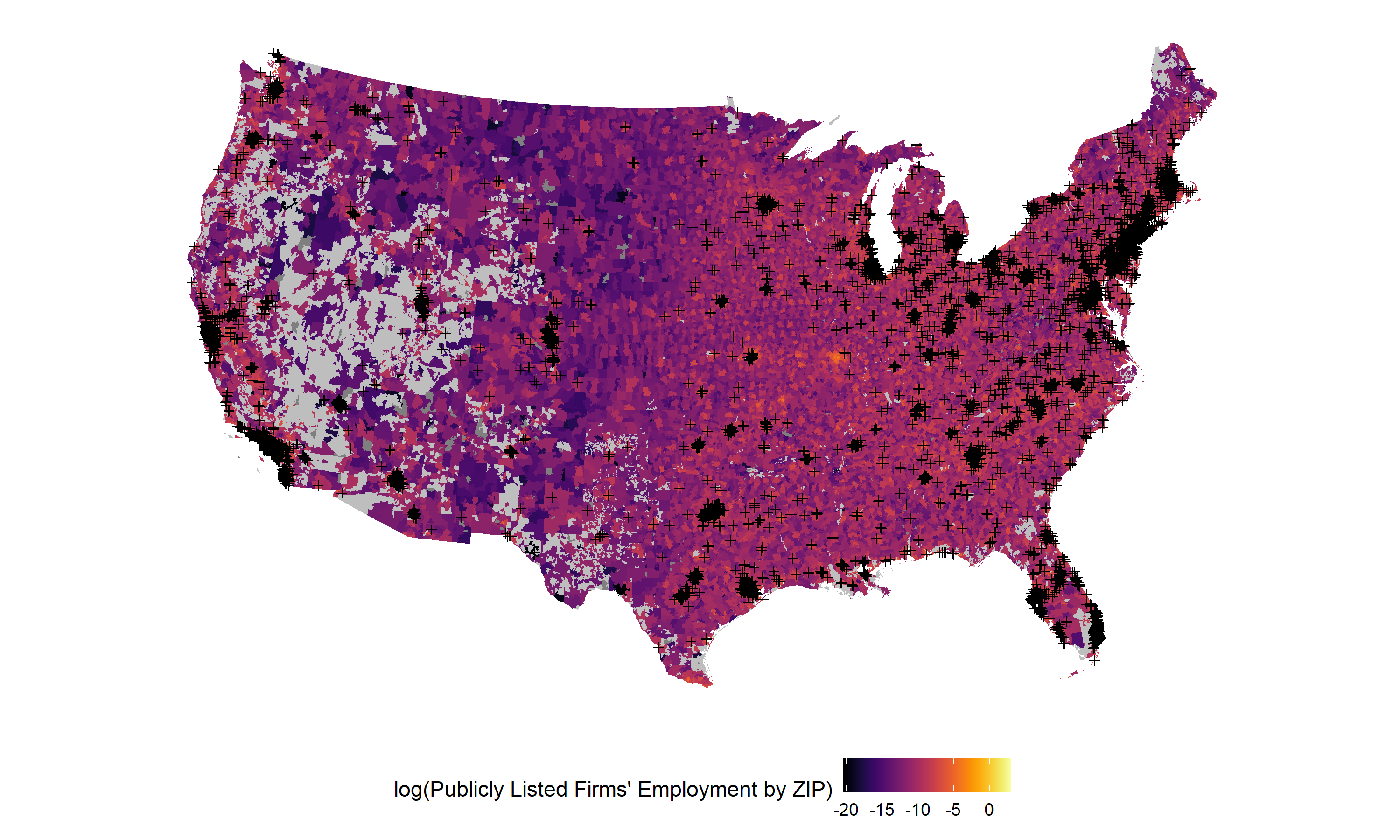
(a) Geographic Distribution of the Employment of Establishments of Publicly-Listed Companies

This map presents the number of years with at least one wildfire for each 5-digit ZIP code, between 2000 and 2018. Fire perimeters from the National Interagency Fire Center. ZIP code boundaries from the Census’ Zip Code Tabulation Areas. In the paper’s regressions, fires are recorded at daily frequency.

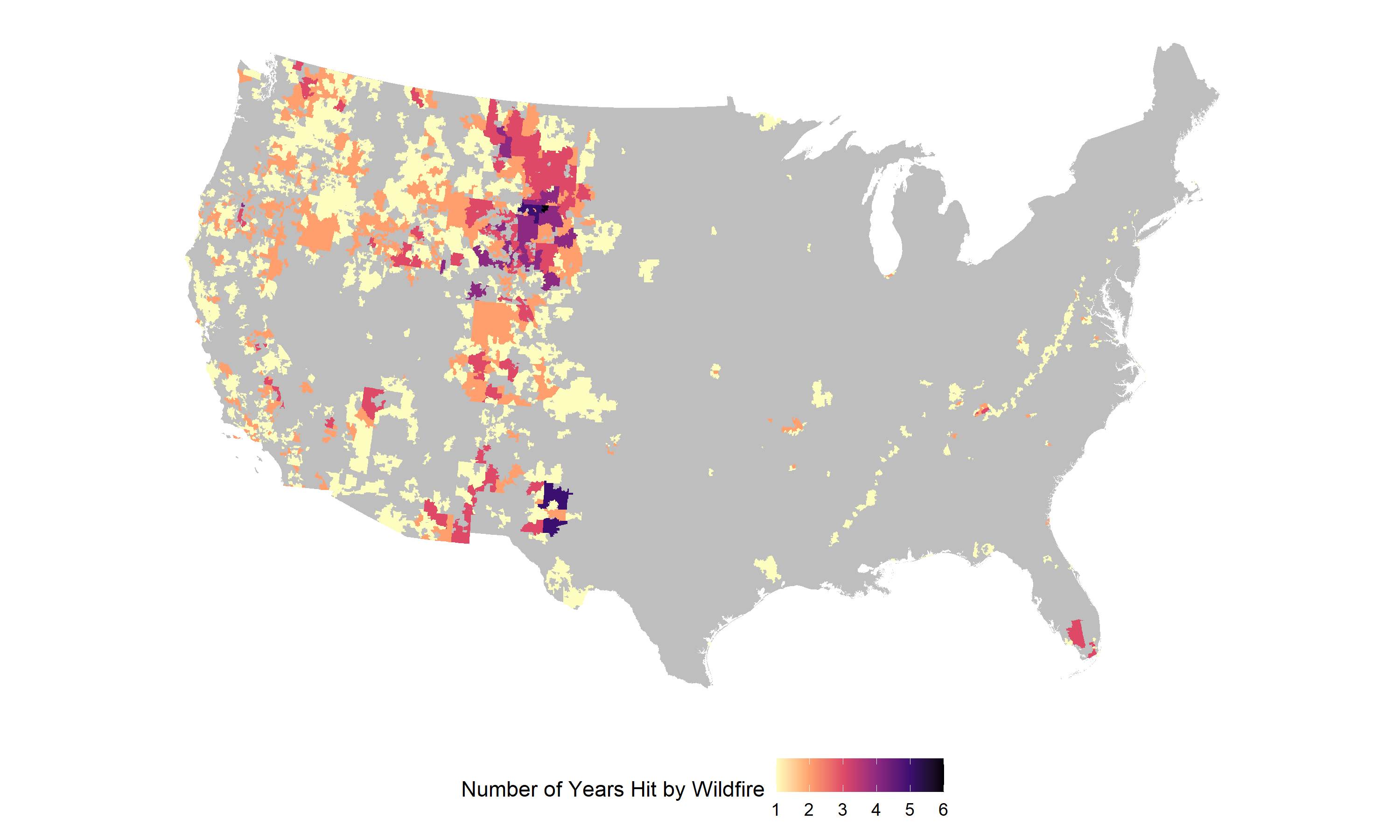
(b) Geographic Distribution of 2000–2018 Wildfires

Figure 2: The Risk Neutral Distribution of PG&E during the October 2017 Wildfires

These four figures display the risk neutral distribution obtained using the convexity of option prices with respect to the strike, as in breeden1978prices. The practical implementation of this recovery is based on arbitrage-free option prices and a local polynomial regression, a method similar to ait2003nonparametric described in Section 3.2.

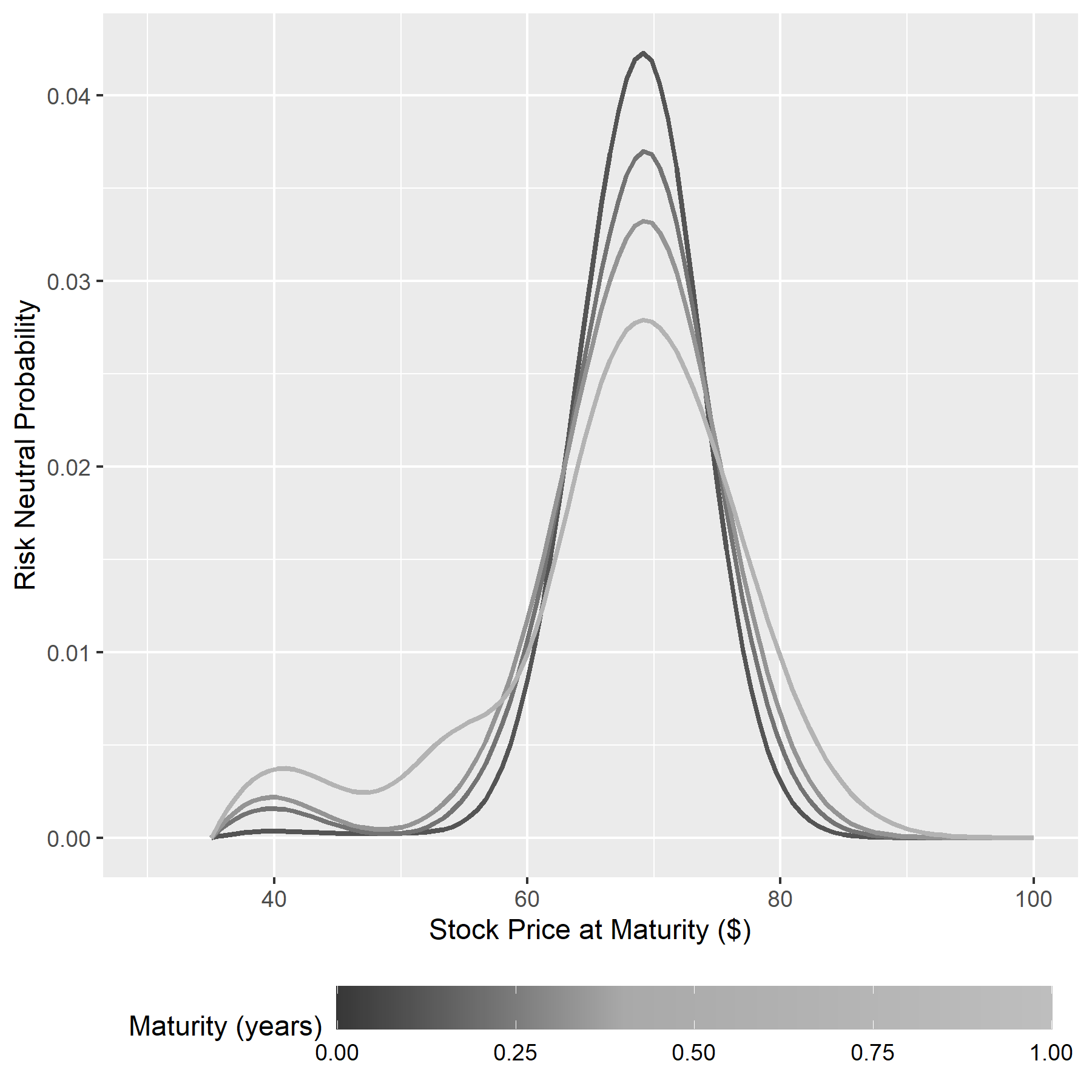
(a) September 22, 2017

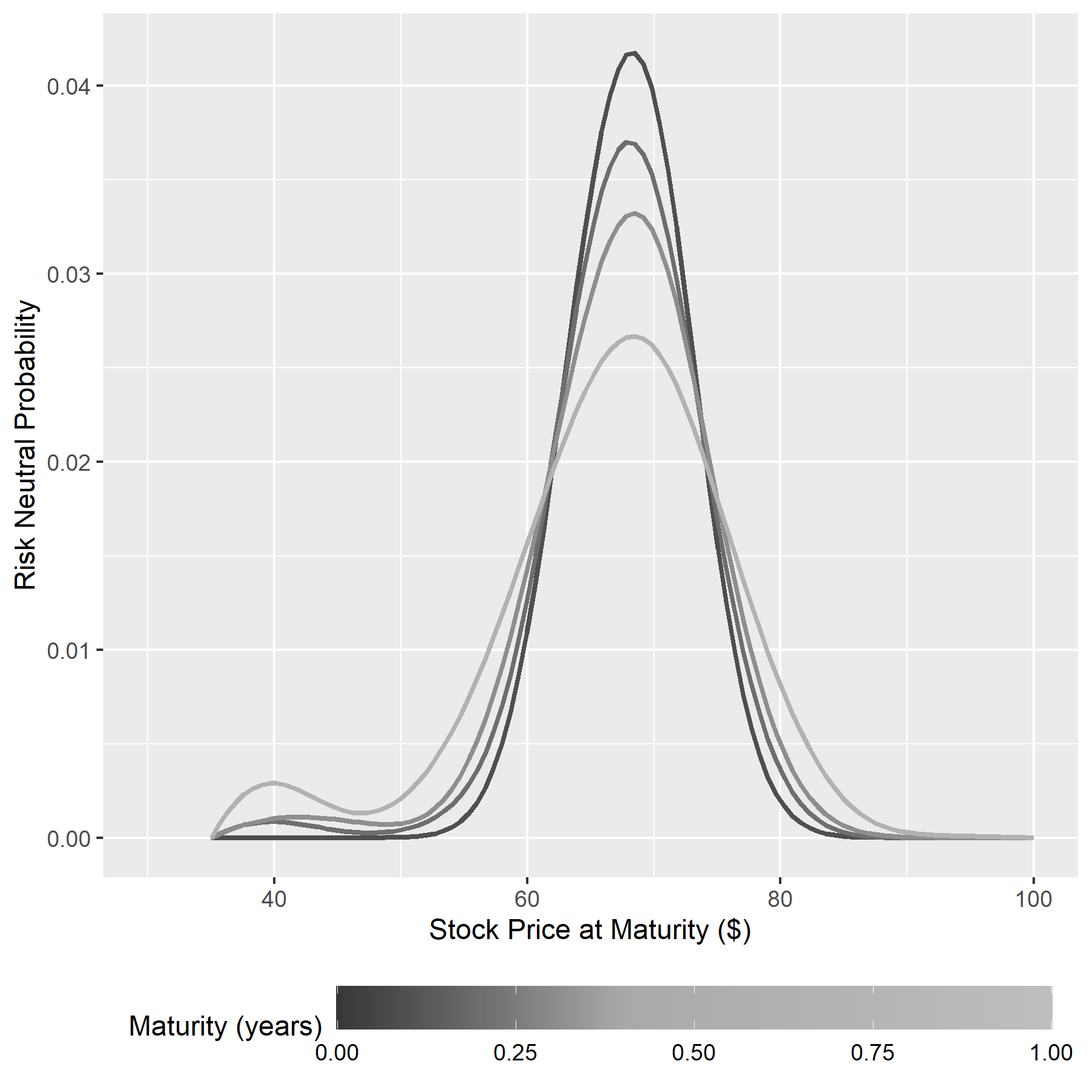
(b) September 27, 2017

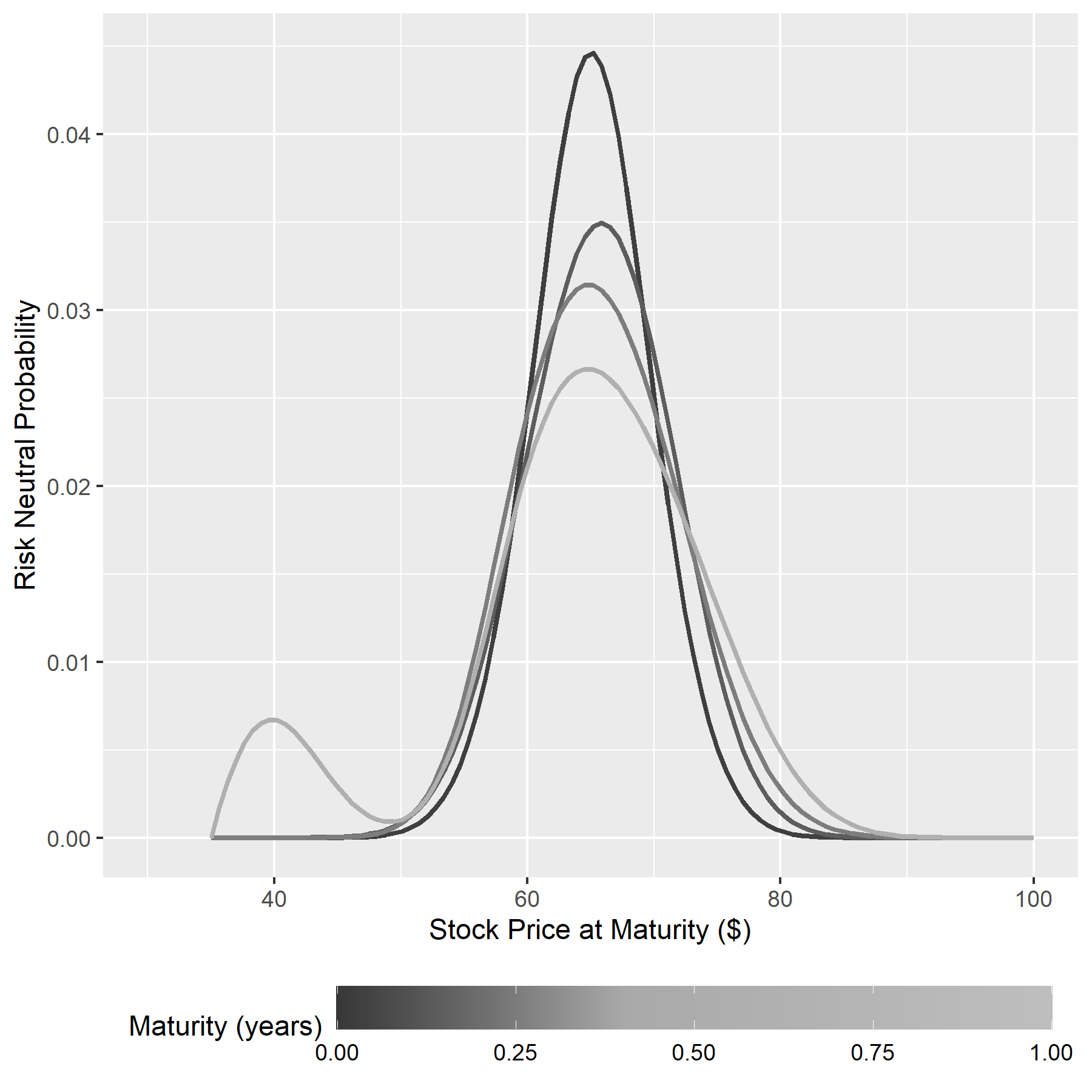
(c) October 12, 2017

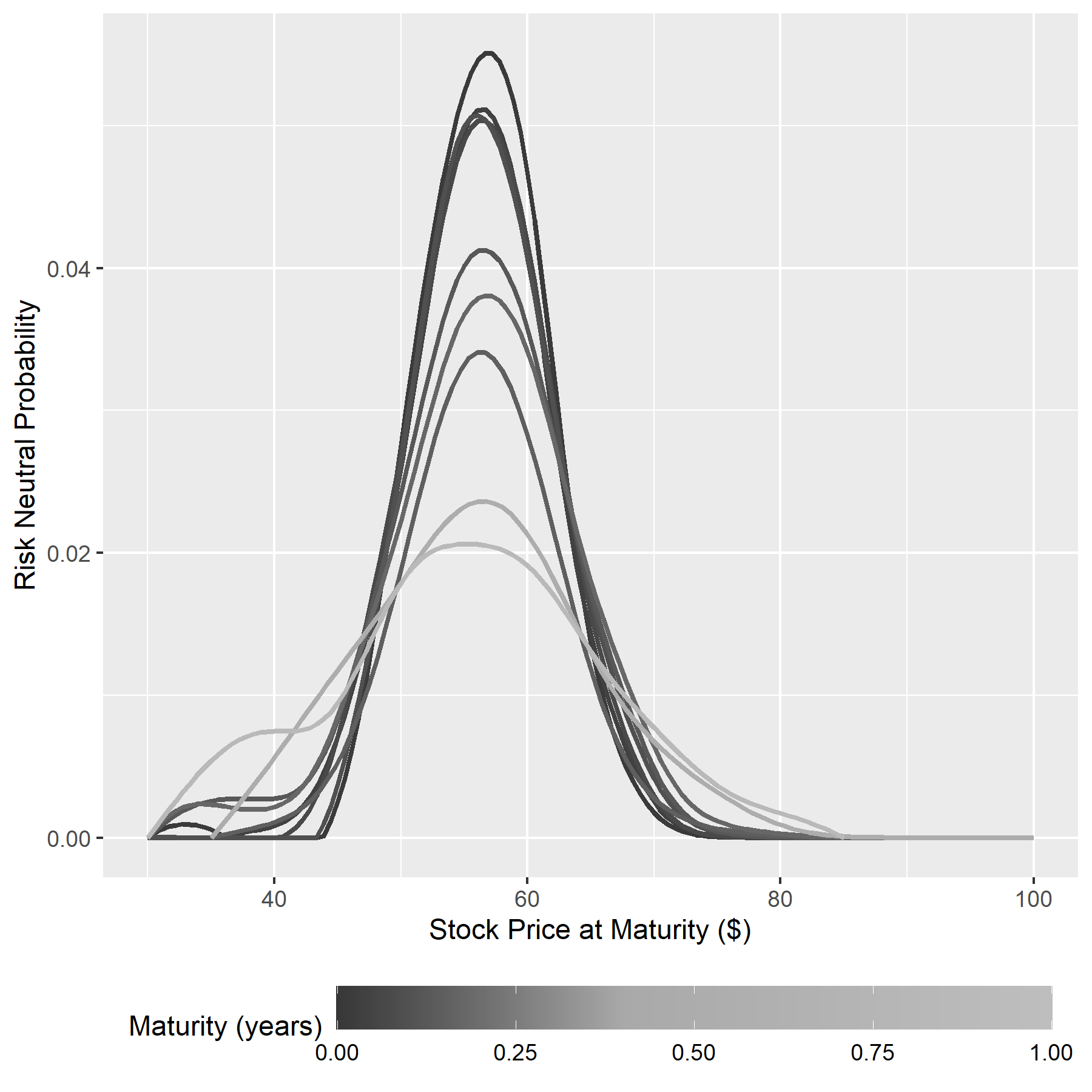
(d) November 7, 2017

Figure 3: Impact of Wildfires on the Risk Neutral Distribution

These figures present the regression of the risk neutral distribution implied by Out of The Money (OTM) puts and calls, on the following covariates: (1) indicators for the 100 moneyness bins, (2) interactions between the treatment – exposure to a wildfire – and the 100 moneyness bins, (3) firm$\times$moneyness and day fixed effects. The points correspond to (2), the interaction between the treatment and the 15 moneyness bins. Standard errors at 95% are double-clustered at the firm and day levels.

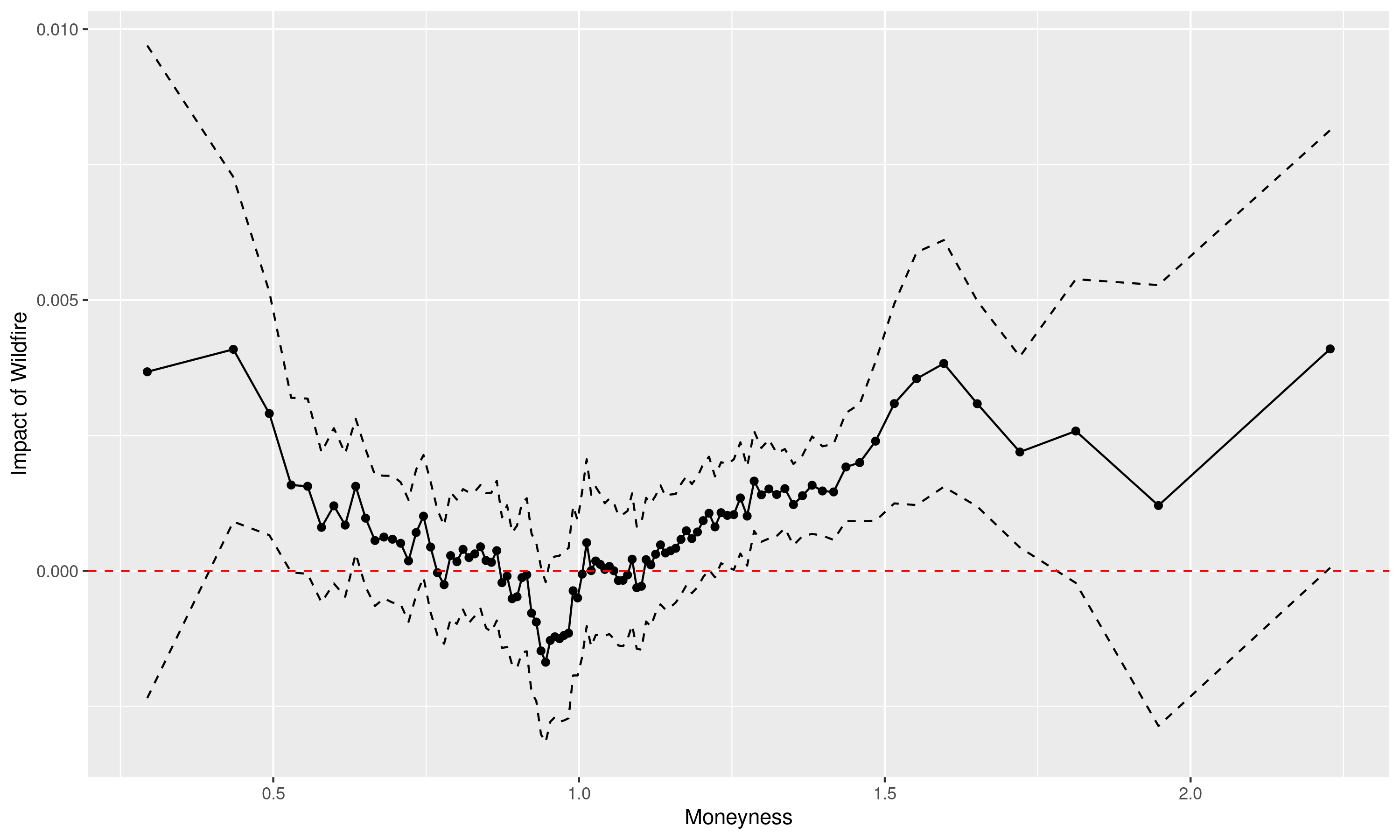
(a) Treatment Effect on Risk Neutral Probabilities, Panel Data with Firm$\times$Moneyness and Day Fixed Effects, 100 Moneyness Bins

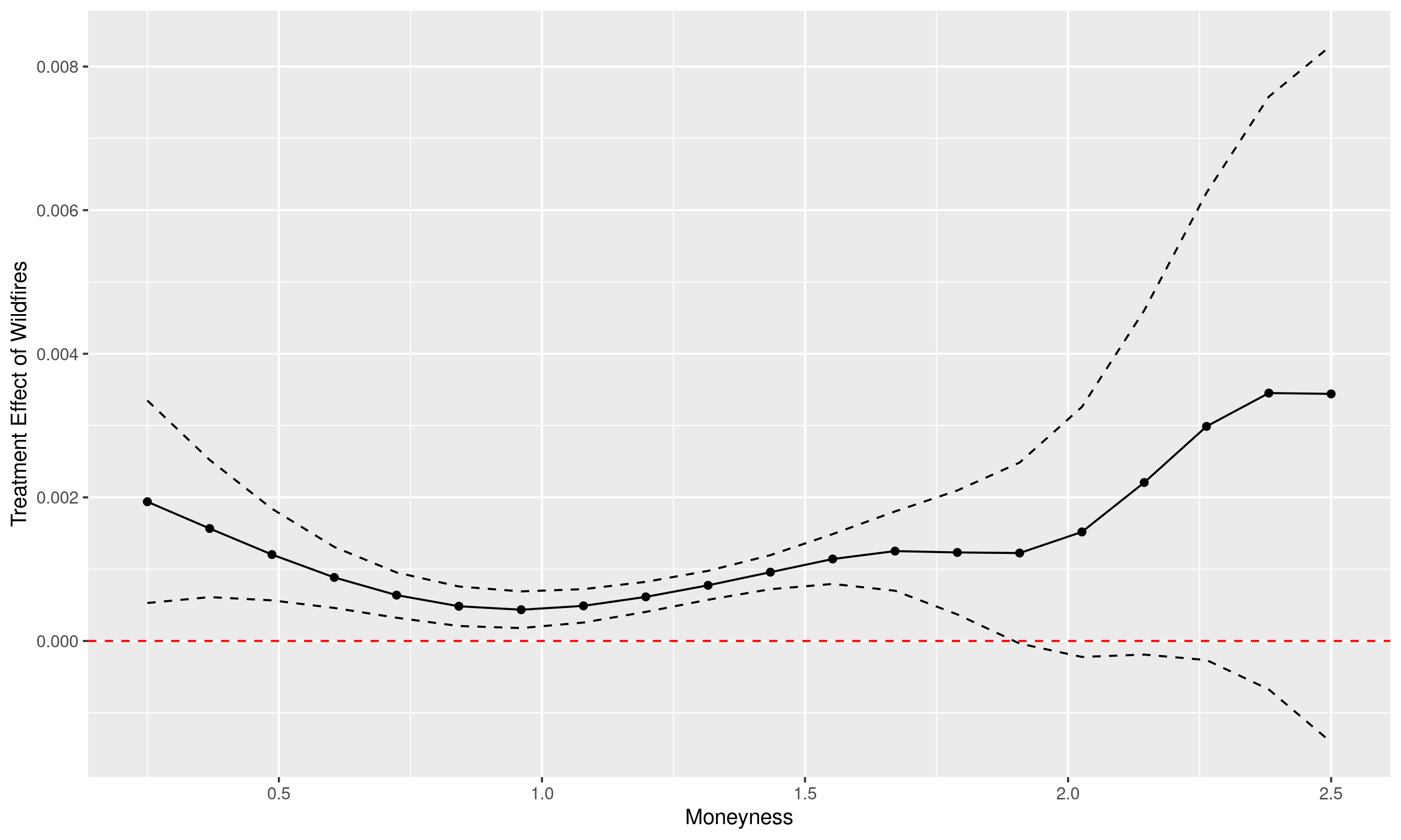
(b) Treatment Effect on Risk Neutral Probabilities, Local Polynomial Regression, Bandwidth=20

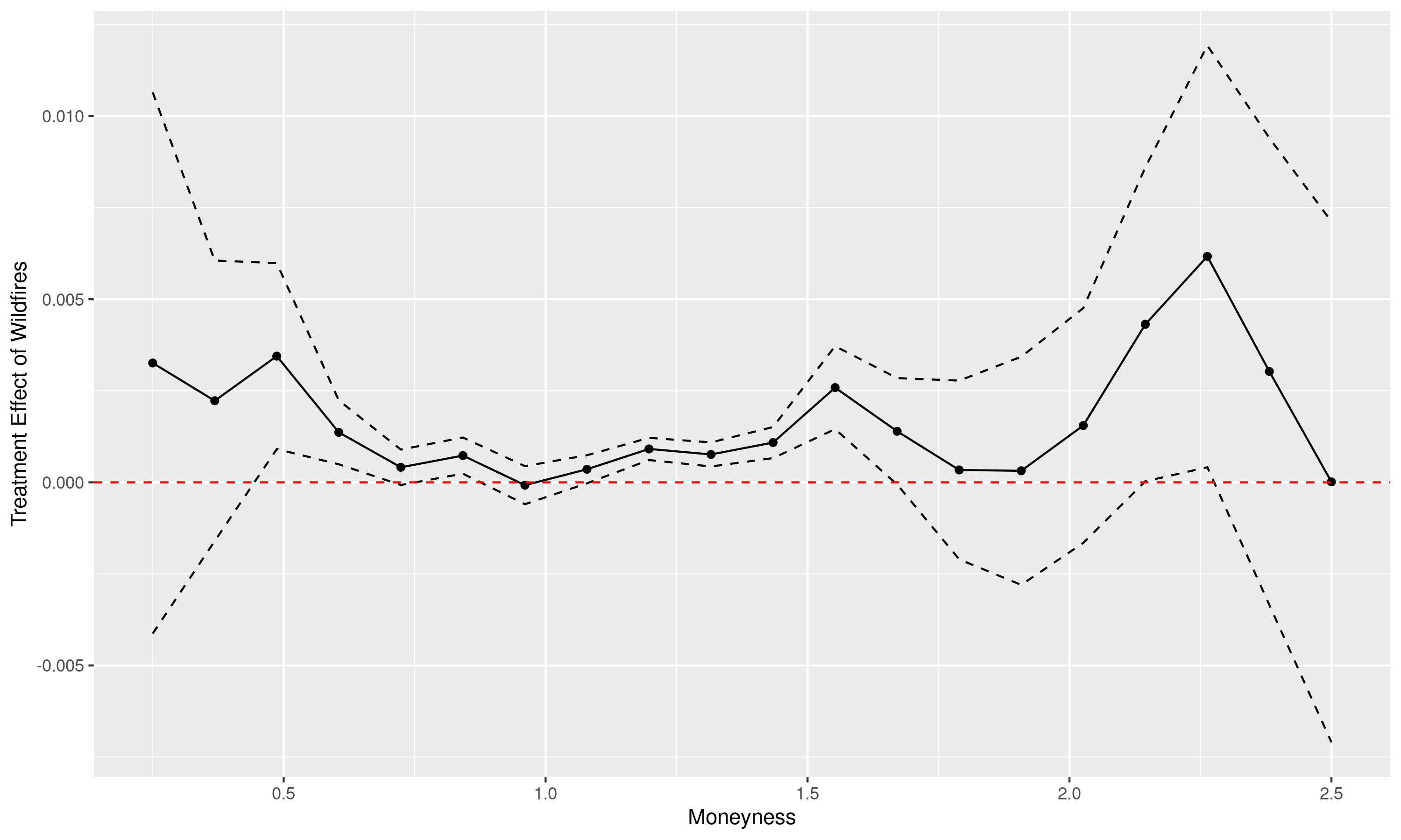
(c) Treatment Effect on Risk Neutral Probabilities, Local Polynomial Regression, Bandwidth=5

Figure 4: By Industry – Impact of Wildfires on the Risk Neutral Distribution

These figures present the regression of the risk neutral distribution implied by Out of The Money (OTM) puts and calls, for three separate NAICS industries. Each point is the estimate of the impact of wildfires on the risk neutral probabilities, controlling for firm$\times$moneyness and day fixed effects.

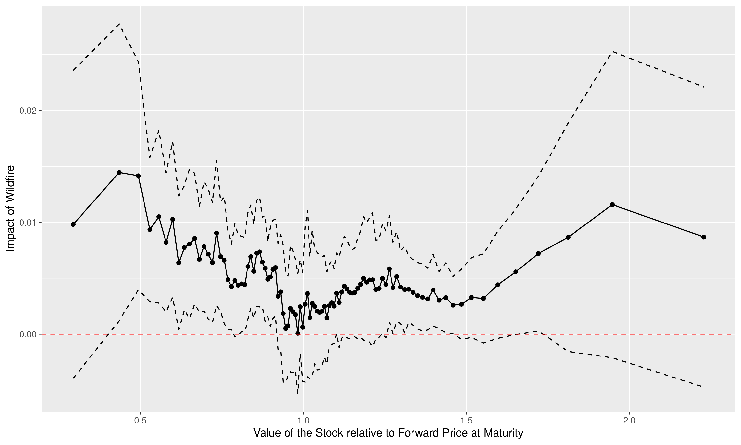
(a) NAICS 4 - Trade, Transportation and Warehousing

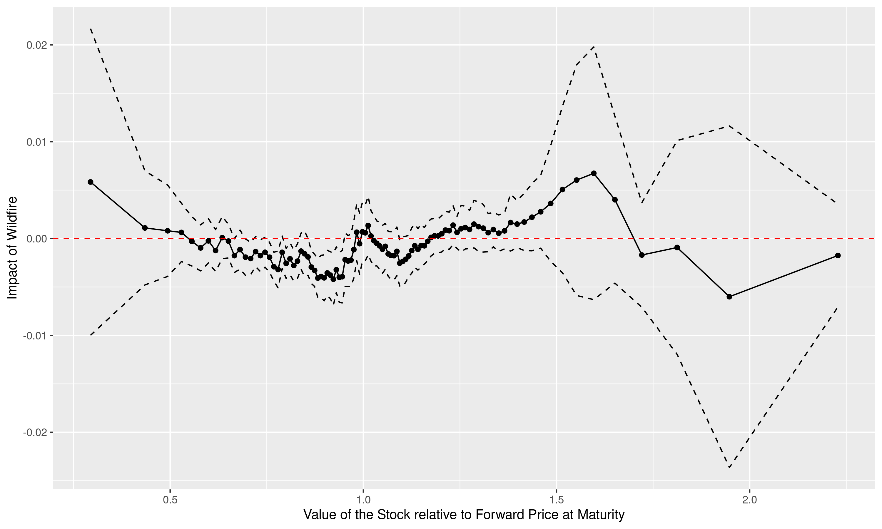
(b) NAICS 5 – Finance, Insurance, Real Estate

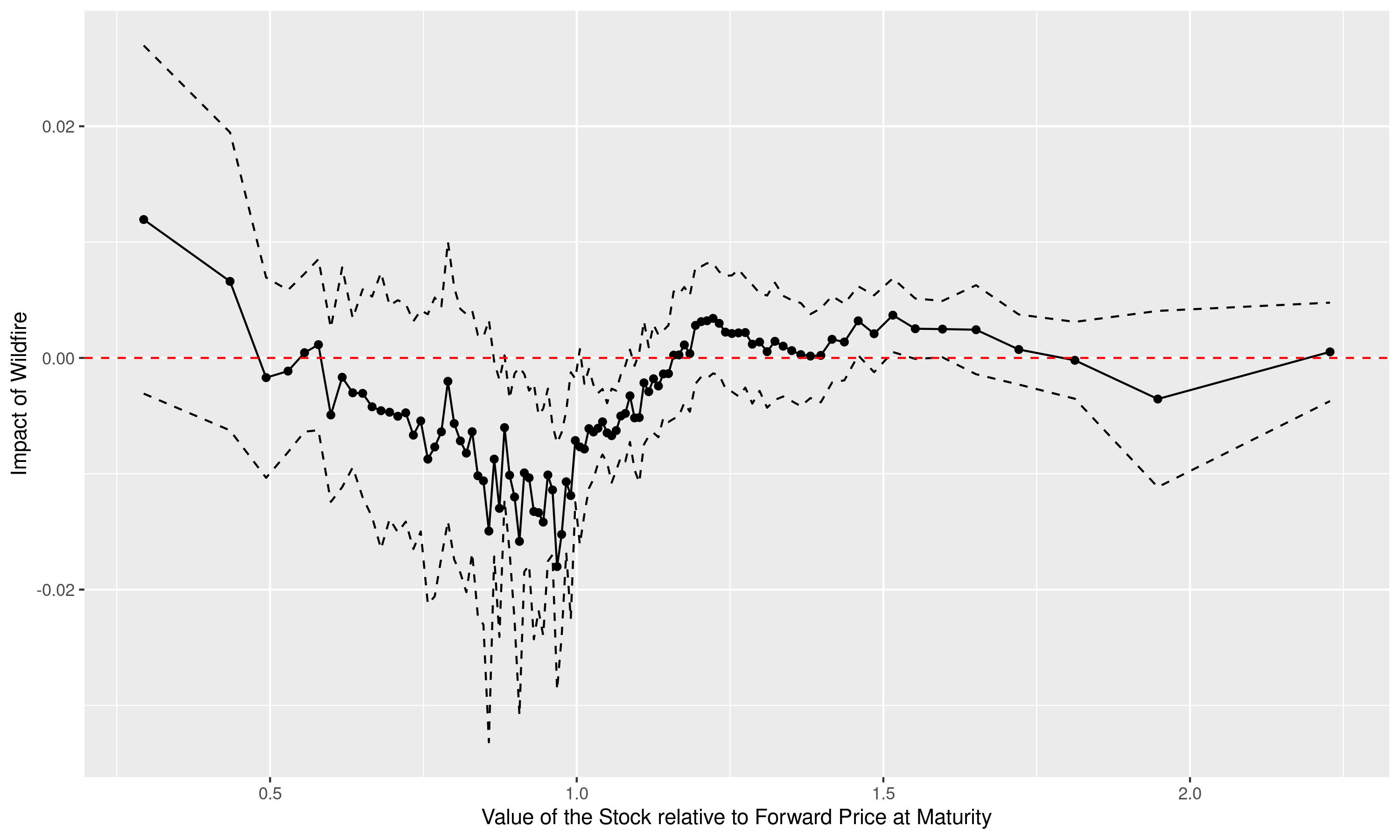
(c) NAICS 7 – Entertainment, Recreation, Accomodation, Food Services

Dotted lines are clustered standard errors at 95%. Black dots are the coefficients of a 2-way fixed effect regression with firm$\times$moneyness and day fixed effects.

Figure 5: By Maturity: Impact of Wildfires on The Risk Neutral Distribution, Panel Data Evidence

These graphs present the non-parametric impact of a wildfire on the risk neutral distribution, estimated using the longitudinal panel of risk neutral probabilities, controlling for day and firm$\times$moneyness fixed effects. Risk neutral probabilities (the dependent variable) are implied by each firm’s daily surface of call prices. Risk neutral probabilities are derived using breeden1978prices approach, implemented using ait2003nonparametric method.

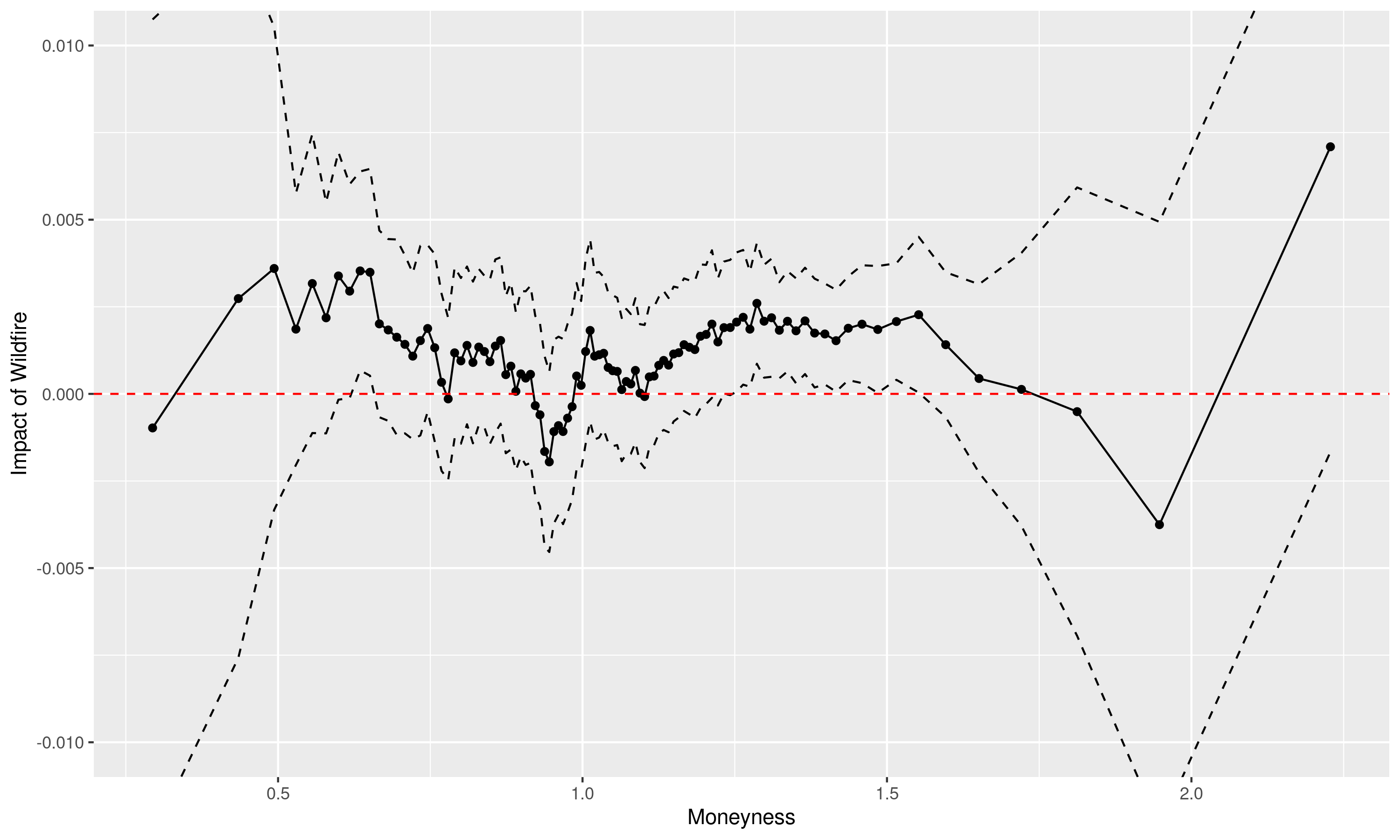
(a) Treatment Effect, Maturity Below the Median

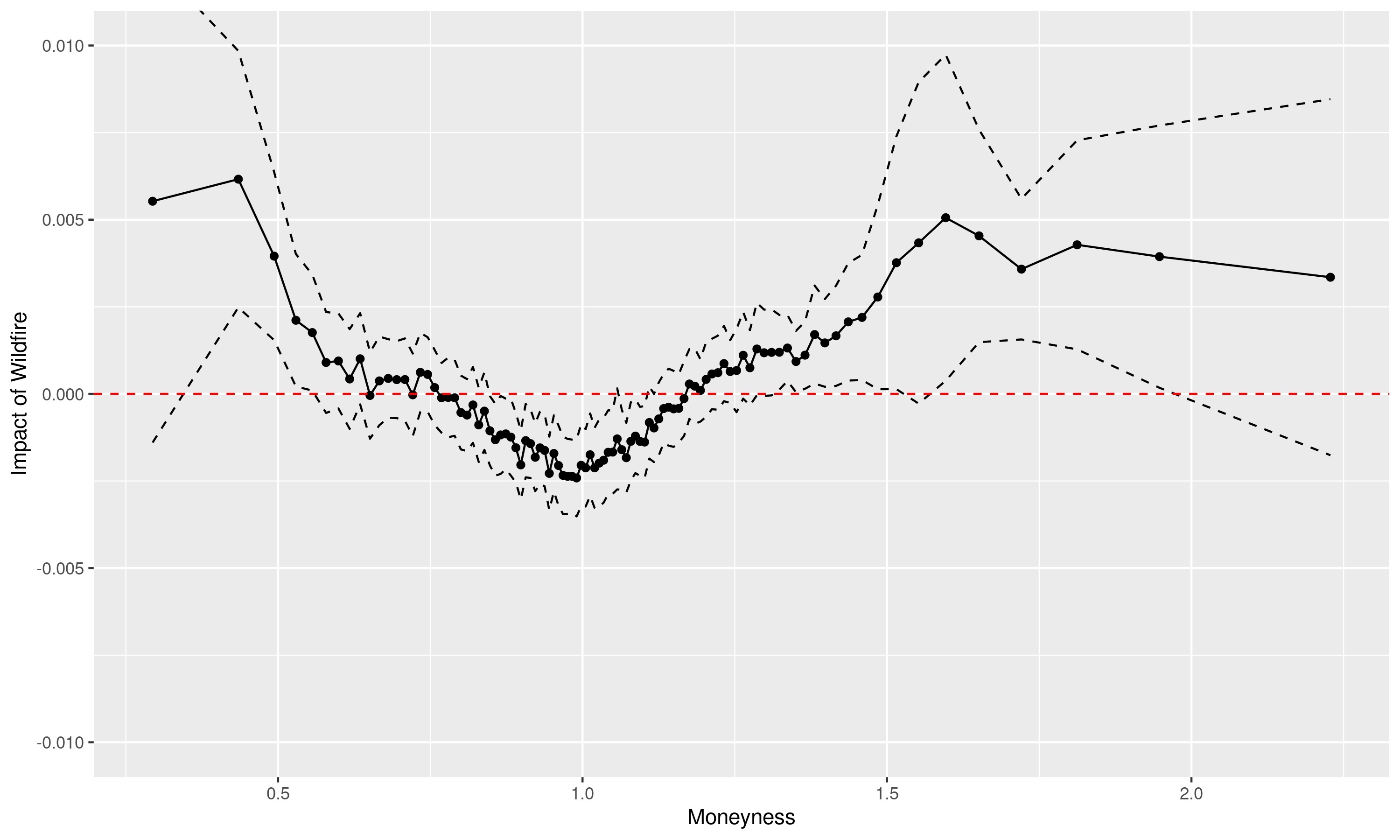
(b) Treatment Effect, Maturity Above the Median

Dotted lines are clustered standard errors at 95%. Black dots are the coefficients of a 2-way fixed effect regression with firm$\times$moneyness and day fixed effects.

Figure 6: The Volatility Surface of PG&E Before and During the October 2017 Northern California wildfires

The implied volatility surface is flat when the underlying stock follows a Geometric Brownian Motion. Here, in contrast, data from PG&E before, during, and after the October 2017 wildfires displays a steepening implied volatility smile. Results are described in Section 4.2.

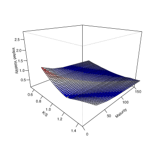
(a) September 22, 2017

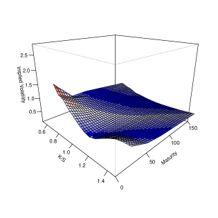
(b) September 27, 2017

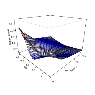
(c) October 12, 2017

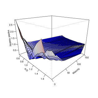
(d) November 7, 2017

Implied volatility from OptionMetrics, obtained using cox1979option binomial-tree approach for American options.

Figure 7: The Impact of Wildfires on the Volatility Smile: Non-Parametric Approach

These four figures present the estimation of the non-parametric specification (12), using both in the money and out of the money options. Implied volatilities are orthogonalized with respect to firm and day fixed effects. A local polynomial regression then regresses orthogonalized implied volatilities on strike and maturity in the control and the treatment groups. Figure (a) presents the IV surface in the control group, denoted $g$. Figure (b) presents the treatment effect, denoted $\Delta g$. Hence the IV surface in the treatment group is $g+\Delta g$. Figure (c) presents a cross section for calls of 3-day maturity. Figure (d) presents the cross section for calls of 11-day maturity. Cross sections of puts display similar results. Cross sections of option IVs with longer maturities display similar results as for the 11-day maturity.

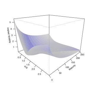
(a) IV Surface, Control Group $g$

(b) IV Surface, Treatment Effect, $\Delta g$

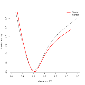
(c) IV Cross Section, Calls, 3-Day Maturity

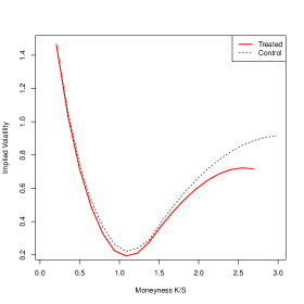
(d) IV Cross Section, Calls, 11-Day Maturity

Figure 8: Identifying Investors’ Marginal Utility of Wildfire Shocks: State Prices from the Ratio of the Risk Neutral Distribution vs. the Physical Distribution, the PG&E Case

In the two upper panels, the bold line is the risk neutral distribution $f^{*}$ on September 22nd (before the fires) and October 12th (during the fires), as obtained using the method of Section 5.1. The dotted lines is the physical distribution $f$ assuming backward-looking expectations. Three approaches for building the physical distribution are described in Section 5.1. The two bottom panels present the pricing kernel, obtained by taking the ratio $f^{*}/f$ of the RND and the physical distribution.

(a) September 22, 2017

(b) October 12, 2017

(c) Pricing Kernel, Backward-Looking Expectations

(d) Pricing Kernel, Backward-Looking Expectations

$\gamma^{w}=-S_{T}^{w}\frac{\zeta^{\prime}(S_{T}^{w})}{\zeta(S_{T}^{w})}\simeq 6.19$           $\gamma^{w}=-S_{T}^{w}\frac{\zeta^{\prime}(S_{T}^{w})}{\zeta(S_{T}^{w})}\simeq 4.56$

Figure 9: Distribution of the Elasticity $\gamma_{j}^{w}$ of State Prices w.r.t. Wildfire-Exposed Stocks

This figure presents the distribution of estimated firm-level elasticity of state prices (investors’ marginal utility) parameters $\gamma_{j}^{w}$ with respect to the value of wildfire-exposed stocks $S_{T}^{w}$. This is done using regression (22), i.e.by regressing $\log f^{*}(S_{j,T}^{w})-\text{log}f(S_{j,T}^{w})-r_{t,T}(T-t)$ on $\log$ moneyness for each firm separately. $f^{*}$ is the risk neutral distribution obtained using option prices and the breeden1978prices approach; $f$ is the physical distribution, obtained by using the estimated GARCH-Wildfire process separately for each firm and forecasting $S_{jt}^{w}$ using the time series of pre-wildfire returns. $r_{t,T}$ is the risk-free interest rate, calibrated using ICE’s LIBOR. $T$ is the maturity of the option.

For most firms, investors’ marginal utility declines when the value of the wildfire stock $S_{T}^{w}$ is higher, consistent with consumer theory, $\gamma^{w}>0$ . Estimates left of the red dotted line exhibit the pricing kernel puzzle, but 87% of firms do not exhibit such a puzzle.

(i) Distribution of $\hat{\gamma}_{j}^{w}$

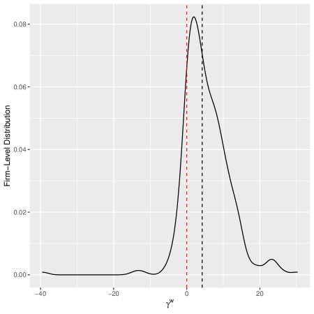
(ii) Descriptive Statistics

Point Estimate (firm-level)	Mean	S.D.	P25	P50	P75	$1(\gamma)<0$	J	N
$\widehat{\gamma_{j}^{w}}$	5.29	6.38	1.34	4.37	8.56	0.13	311	1,479,976
t-Statistic	Mean	S.D.	P25	P50	P75	$1(t)<-1.96$	J	N
$\widehat{\gamma_{j}}/\widehat{SE_{j}}$	11.07	10.88	3.40	10.38	17.56	0.08	311	1,479,976

$J$: number of distinct wildfire-exposed firms with moneyness ranging between 0.5 and 1.5 times the forward price. $N$: number of day $\times$ strike $\times$ firm observations, wildfire-exposed firms. $1(\gamma)<0$ : exhibits a pricing kernel puzzle (point estimate). $1(t)<-1.96$: the pricing kernel puzzle is statistically significant.

Table 2: The Impact of Wildfires on the Volatility Smile : Panel Data Evidence, 2000-2018

These two tables present the impact of a wildfire, on the days of the wildfire, on the implied volatility skew for puts (upper panel) and for calls (lower panel). The specification is a linear panel fixed effect regression, as in (11) with double-clustered standard errors. $S$ is the forward price. We take the square root of maturity, as in dumas1998implied and consistent with the empirical term structure of implied volatilities.

	Implied Volatility, Puts
	(1)	(2)	(3)	(4)
Constant	1.093***
	(0.001)
Moneyness $K/S$	$-$0.342***	$-$0.394***	$-$0.355***	$-$0.413***
	(0.001)	(0.022)	(0.023)	(0.032)
Maturity $\sqrt{T}$	$-$0.044***	$-$0.051***	$-$0.044***	$-$0.051***
	(0.000)	(0.001)	(0.002)	(0.002)
$K/S$ $\times$ $\sqrt{T}$	0.014***	0.014***	0.014***	0.013***
	(0.000)	(0.002)	(0.002)	(0.002)
Treated	0.131***	0.151**	0.124**	0.145**
	(0.006)	(0.063)	(0.046)	(0.070)
Treated $\times$ $K/S$	$-$0.197***	$-$0.176**	$-$0.184***	$-$0.159**
	(0.006)	(0.070)	(0.052)	(0.076)
Treated $\times$ $\sqrt{T}$	$-$0.015***	$-$0.015**	$-$0.014**	$-$0.014**
	(0.001)	(0.005)	(0.004)	(0.006)
Treated $\times$ $K/S$ $\times$ $\sqrt{T}$	0.016***	0.016**	0.016***	0.016**
	(0.001)	(0.006)	(0.005)	(0.006)
Firm fixed effects		Yes		Yes
Day fixed effects			Yes	Yes
$N$	16,842,463	16,842,463	16,842,463	16,842,463
$R^{2}$	0.109	0.309	0.146	0.352
	Implied Volatility, Calls
	(1)	(2)	(3)	(4)
Constant	0.509***
	(0.001)
Moneyness $K/S$	0.219***	0.066**	0.206***	0.048
	(0.001)	(0.023)	(0.020)	(0.031)
Maturity $\sqrt{T}$	$-$0.003***	$-$0.016***	$-$0.003**	$-$0.017***
	(0.000)	(0.002)	(0.002)	(0.002)
$K/S$ $\times$ $\sqrt{T}$	$-$0.026***	$-$0.020***	$-$0.026***	$-$0.020***
	(0.000)	(0.002)	(0.001)	(0.002)
Treated	0.139***	0.148*	0.134**	0.148
	(0.006)	(0.087)	(0.049)	(0.091)
Treated $\times$ $K/S$	$-$0.194***	$-$0.173*	$-$0.180***	$-$0.155
	(0.006)	(0.092)	(0.047)	(0.095)
Treated $\times$ $\sqrt{T}$	$-$0.016***	$-$0.015**	$-$0.015***	$-$0.013*
	(0.001)	(0.007)	(0.004)	(0.008)
Treated $\times$ $K/S$ $\times$ $\sqrt{T}$	0.017***	0.015**	0.017***	0.015*
	(0.001)	(0.007)	(0.004)	(0.008)
Firm fixed effects		Yes		Yes
Day fixed effects			Yes	Yes
$N$	16,839,339	16,839,339	16,839,339	16,839,339
$R^{2}$	0.091	0.280	0.127	0.321

***: significant at 1%, **: significant at 5%, *: significant at 10%.

Table 3: By Industry: Control and Treatment Group

These two tables present industry-level statistics on the share of firm $\times$ date observations treated, i.e. exposed to a wildfire, with either more than 10% of establishments, employment, or sales in the perimeter of a wildfire between 2000 and 2018. The first table displays overall statistics for the 238 6-digit NAICS codes. 74.4% of such industries have at least one treated firm $\times$date observation, and on average 1.5% of observations are treated. The bottom table presents the industries ranked in decreasing order of the share of observations treated.

Share of Industries	Fraction Treated						Number of Industries
with Treated Firm(s)	Average	P10	Median	P90	P95	P99	6-Digit NAICS
0.744	0.015	0.000	0.012	0.035	0.043	0.064	238

(a) Industry Statistics

NAICS Code	2017 NAICS Title	Fraction Treated	Distinct Firm $\times$ Dates
621610	Home Health Care Services	0.08	251
332993	Ammunition (except Small Arms) Manufacturing	0.07	178
424720	Petroleum and Petroleum Products Merchant Wholesalers (except Bulk Stations and Terminals)	0.07	461
335999	All Other Miscellaneous Electrical Equipment and Component Manufacturing	0.06	281
722320	Caterers	0.05	300
211130	Natural Gas Extraction	0.05	351
517311	Wired Telecommunications Carriers	0.05	765
532490	Other Commercial and Industrial Machinery and Equipment Rental and Leasing	0.05	259
561920	Convention and Trade Show Organizers	0.05	522
333999	All Other Miscellaneous General Purpose Machinery Manufacturing	0.05	397
621512	Diagnostic Imaging Centers	0.04	404
447190	Other Gasoline Stations	0.04	412
451211	Book Stores	0.04	278
334515	Instrument Manufacturing for Measuring and Testing Electricity and Electrical Signals	0.04	285
424110	Printing and Writing Paper Merchant Wholesalers	0.04	285
221310	Water Supply and Irrigation Systems	0.04	1125
483112	Deep Sea Passenger Transportation	0.04	1078
316998	All Other Leather Good and Allied Product Manufacturing	0.04	470
445110	Supermarkets and Other Grocery (except Convenience) Stores	0.04	315
541614	Process, Physical Distribution, and Logistics Consulting Services	0.04	315

(b) Share of Firm $\times$ Date Treated, by Industry

	Share of Industries with	Statistically Significant
	Steepening Volatility Smile	at 90%	at 95%	at 99%
Out-of-the-money Puts	0.657	0.600	0.571	0.572
Out-of-the-money Calls	0.257	0.243	0.243	0.243

(c) Treatment Effects by Industry

Table 4: Permanent Effects of a Wildfire on Options’ Implied Volatility Smile

This table estimates the permanent effects of wildfires on option implied volatilities. ”After First Wildfire” is equal to 1 on any day after the first wildfire affecting the publicly traded company. ”After Last Wildfire” is equal to 1 on any day after the first wildfire affecting the company. Other covariates are similar to the linear specification of table 2 and specification (11). As in Table 2, standard errors are double-clustered at the firm and day levels. All four regressions include two-way fixed effects.

	Implied Volatility
	Puts	Calls	Puts	Calls
	(1)	(2)	(3)	(4)
Moneyness $K/S$	-0.420***	0.080**	-0.414***	0.067**
	(0.031)	(0.031)	(0.030)	(0.031)
Maturity $\sqrt{T}$	-0.053***	-0.015***	-0.052***	-0.016***
	(0.002)	(0.002)	(0.002)	(0.002)
Moneyness $K/S$ $\times$ Maturity $\sqrt{T}$	0.014***	-0.022***	0.013***	-0.021***
	(0.002)	(0.002)	(0.002)	(0.002)
After First Wildfire	-0.047	0.126**
	(0.062)	(0.056)
After First Wildfire $\times$ Moneyness $K/S$	0.017	-0.152**
	(0.066)	(0.057)
After First Wildfire $\times$ Maturity $\sqrt{T}$	0.005	-0.009**
	(0.005)	(0.004)
After First Wildfire $\times$ Moneyness $K/S$ $\times$ Maturity $\sqrt{T}$	-0.001	0.013**
	(0.005)	(0.004)
After Last Wildfire			-0.016	0.106
			(0.075)	(0.066)
After Last Wildfire $\times$ Moneyness $K/S$			-0.013	-0.132**
			(0.081)	(0.066)
After Last Wildfire $\times$ Maturity $\sqrt{T}$			0.002	-0.008*
			(0.006)	(0.005)
After Last Wildfire $\times$ Moneyness $K/S$ $\times$ Maturity $\sqrt{T}$			0.002	0.011**
			(0.007)	(0.005)
Firm fixed effects	Yes	Yes	Yes	Yes
Day fixed effects	Yes	Yes	Yes	Yes
$N$	16,842,463	16,839,339	16,842,463	16,839,339
$R^{2}$	0.352	0.322	0.352	0.322

***: significant at 1%, **: significant at 5%, *: significant at 10%.

Table 5: Implied Jumps and Stochastic Volatility for Wildfire-Exposed Stocks: US Exchange-Traded Equity Options Exposed to Wildfires

This table presents the estimation of the stochastic volatility and jump parameters implied by the equity options of the publicly-listed firms exposed to wildfires. This is the treatment group of Section 4. We also present the calibration for the control group. Estimation is performed by minimizing the distance between the model-based implied volatilities to the implied volatilities of the treatment group (resp. the control group). The baseline Black and Scholes diffusion without jumps has a mean squared error of 0.703 in the treatment group and 0.677 in the control group.

	Jump Diffusion		Double Exponential Jumps
	merton1976option		kou2004option
	Control	Treatment	Control	Treatment
Volatility ($\sigma$)	0.064	0.003	0.001	0.003
Jump intensity ($\lambda$)	0.148	0.146	0.721	0.428
Mean jump magnitude ($\mu^{s}$)	$-$0.308	$-$1.013	-	-
S.D. of jump magnitude ($\sigma^{s}$)	1.354	1.533	-	-
Probability of an upward jump ($p$)	-	-	0.796	0.743
Mean downward jump ($-1/\eta_{1}$)	-	-	$-$0.908	$-$1.765
Mean upward jump ($1/\eta_{2}$)	-	-	0.378	0.383
Mean Squared Error	0.056	0.066	0.072	0.058

Parameters are calibrated by pricing options using the characteristic function approach. The calibration minimizes the sum of squared deviations between the model and the empirical implied volatilities.

9 Proof of Proposition 1

Proposition.

Sensitivity of State Prices $\zeta_{T}$ to the Terminal Value of the Wildfire-Exposed Stock

When the parameters of the stocks’ stochastic processes $\mu,\alpha,\beta,\sigma,\sigma^{w}$ are constant, when the investor has CRRA preferences $u(w)=\frac{w^{1-\gamma}}{1-\gamma}$, a closed form ties the sensitivity of state prices w.r.t the wildfire-exposed stock to the investor’s risk aversion w.r.t. wealth:

$$\gamma^{w}=(q^{w}+\rho\frac{\sigma}{\sigma^{w}}q)\gamma$$ (28)

where $q^{w}$ the share of wealth invested in the wildfire-exposed stock, $q$ is the share of wealth invested in the diversified portfolio; $\rho$ is the correlation between the returns on the wildfire stock and the diversified portfolio, $\rho=\beta\sigma/\sqrt{\beta^{2}\sigma^{2}+(\sigma^{w})^{2}}$; $\sigma$ and $\sigma^{w}$ the volatilities of the stock and the wildfire-exposed stock respectively.

Proof.

This framework corresponds to merton1969lifetime continuous-time portfolio problem with two risky assets. Risk aversion is the elasticity of the pricing kernel w.r.t. either wealth (for $\gamma$) or the wildfire-exposed stock (for $\gamma^{w}$):

$$\gamma=-\frac{d\log\zeta_{T}}{d\log W_{T}},\qquad\gamma^{w}=-\frac{d\log E(\zeta_{T}|S_{T}^{w})}{d\log S_{T}^{w}}$$ (29)

In merton1969lifetime, the portfolio share $q_{t}$ invested in the index and the share invested in the wildfire-exposed stock $q_{t}^{w}$ are constant, $q_{t}=q$ and $q_{t}^{w}=q^{w}$. The shares held in the wildfire-exposed stock and in the index are obtained using the Hamilton-Jacobi-Bellman equation:

$$q^{w}=\frac{\alpha+\beta\mu-r}{\gamma(\sigma^{w})^{2}},\qquad q=\frac{\mu-r}{\gamma\sigma^{2}}-q^{w}\beta$$ (30)

where $\gamma=-\frac{V_{W}}{V_{WW}W}$ is the Arrow-Pratt relative risk aversion with respect to wealth, $V_{W}=\frac{\partial V}{\partial W}$, $V_{WW}=\frac{\partial^{2}V}{\partial W^{2}}$. Such risk aversion is simply the scalar $\gamma$ when the investor’s utility is CRRA.

Terminal wealth conditional on the value $S_{T}^{w}$ of the wildfire stock is a function of the shares $q$, $q^{w}$ invested and the paths of the Brownians:

$$W_{T}=W_{0}e^{(q(\mu-r)+q^{w}(\alpha+\beta\mu-r)+r-\frac{1}{2}q^{2}\sigma^{2})t}e^{(q+\beta q^{w})\sigma(B_{T}-B_{0})}e^{q^{w}\sigma^{w}(B_{T}^{w}-B_{0}^{w})}$$ (31)

and $\zeta_{T}=u^{\prime}(W_{T})=W_{T}^{-\gamma}$, hence the log of the pricing kernel:

$$\log\zeta_{T} =-\gamma\log W_{0}-\gamma(q(\mu-r)+q^{w}(\alpha+\beta\mu-r)+r-\frac{1}{2}q^{2}\sigma^{2})t$$

$$\quad\quad\quad\quad\quad\quad\quad-\gamma(q+\beta q^{w})\sigma(B_{T}-B_{0})+q^{w}\sigma^{w}(B_{T}^{w}-B_{0}^{w})$$ (32)

this can also be rewritten as a function of the values of the stocks. To see this, first express the terminal values of $S_{T}$ and $S_{T}^{w}$:

$$\log S_{T} =\log S_{0}+(\mu-\frac{1}{2}\sigma^{2})t+\sigma(B_{T}-B_{0})$$ (33)

$$\log S_{T}^{w} =\log S_{0}^{w}+(\alpha+\beta\mu-\frac{1}{2}\beta^{2}\sigma^{2}-\frac{1}{2}(\sigma^{w})^{2})t+\beta\sigma(B_{T}-B_{0})+\sigma^{w}(B_{T}^{w}-B_{0}^{w})$$ (34)

$(\log S_{T},\log S_{T}^{w})$ is bivariate normal with correlation $\rho$ and with variances $\sigma T$ and $\sigma^{w}T$. The correlation $\rho$ is a function of the beta of the stock and the standard deviations $\rho=\beta\sigma/\sqrt{\beta^{2}\sigma^{2}+(\sigma^{w})^{2}}$. Hence the classic bivariate conditional expectation formula applies. The expected value of $\log S_{T}$ conditional on $S_{T}^{w}$ is $E(\log S_{T})+\rho\frac{\sigma}{\sigma^{w}}(\log S_{T}^{w}-E(\log S_{T}^{w}))$. Hence $d\log E(\zeta_{T}|S_{T}^{w})/d\log S_{T}^{w}=q^{w}+\rho\frac{\sigma}{\sigma^{w}}q$. ∎

Appendix Figure A: Wildfire Exposure Over Time

At daily frequency, these three panels present the log number of establishments, the log number of employees, and the log dollar sales of establishments of listed firms in wildfire perimeters.

(a) Establishments

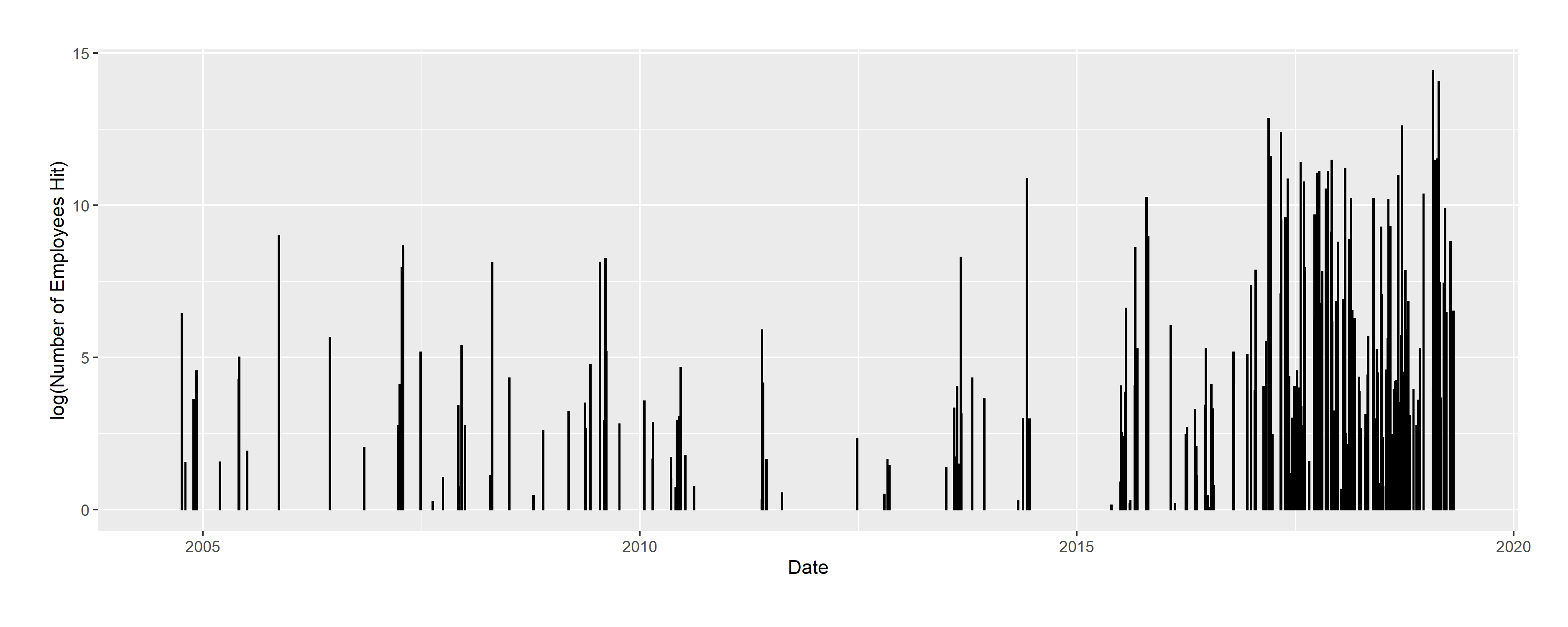
(b) Employment

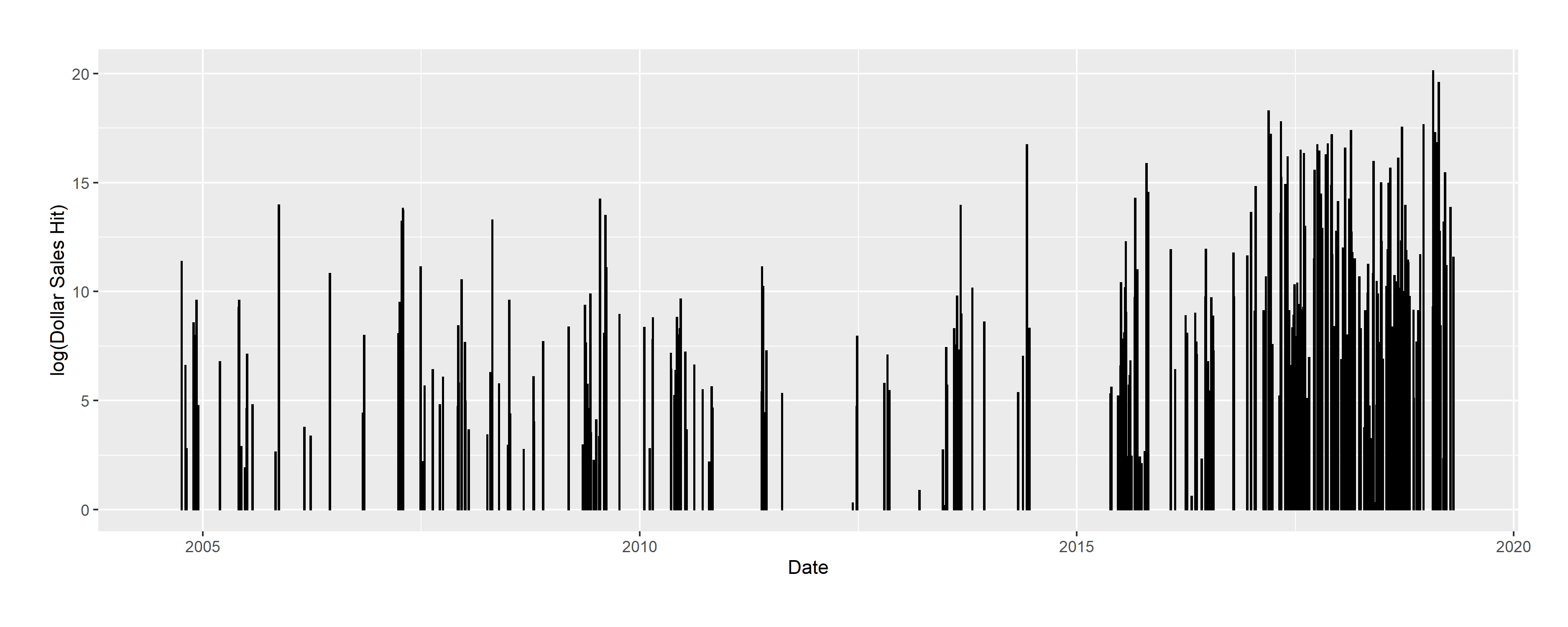
(c) Sales

Appendix Table A: Industries Hit by Wildfires, Ranked by Number of Establishments Hit

For each 6-digit NAICS industry, this table presents the number of establishments, the employment, in thousands, and the sales, in thousands of $, in wildfire perimeters. Wildfire perimeters are as reported by the National Interagency Fire Center. Establishments, employment, and sales as reported by Dun and Bradstreet’s National Establishment Timer Series (NETS). These numbers are cumulative over the 681 days with a wildfire.

		In Wildfire Perimeter At Any Point
		Establishments	Employment	Sales
NAICS	Description	(’000)	(’000)	(’000)
722513	Limited-Service Restaurants	18.1	410.8	21,914.1
522110	Commercial Banking	15.6	189.9	51,623.9
721110	Hotels (except Casino Hotels) and Motels	14.7	156.8	17,780.6
445110	Supermarkets and Other Grocery (except Convenience) Stores	14.5	123.5	29,724.8
519130	Internet Publishing and Broadcasting and Web Search Portals	13.4	75.3	19,953.2
523930	Investment Advice	12.4	17.2	4,580.3
333318	Other Commercial and Service Industry Machinery Manufacturing	12.3	15.1	3,878.0
561621	Security Systems Services (except Locksmiths)	12.2	14.5	3,747.2
324110	Petroleum Refineries	11.4	78.0	93,234.3
722511	Full-Service Restaurants	10.1	264.9	13,746.9
561499	All Other Business Support Services	8.1	12.4	2,776.6
611310	Colleges, Universities, and Professional Schools	7.5	11.5	2,611.0
452319	All Other General Merchandise Stores	6.9	359.4	85,674.0
532120	Truck, Utility Trailer, and RV (Recreational Vehicle) Rental and Leasing	5.8	26.2	5,279.1
531210	Offices of Real Estate Agents and Brokers	5.6	120.1	14,804.7
486110	Pipeline Transportation of Crude Oil	5.5	31.4	29,888.7
446110	Pharmacies and Drug Stores	4.6	87.0	31,673.4
722515	Snack and Nonalcoholic Beverage Bars	3.7	61.0	3,530.2
515210	Cable and Other Subscription Programming	3.4	29.9	10,010.1
523920	Portfolio Management	3.3	69.7	10,801.0

Appendix Table B: Trading of Short-Maturity Options and Wildfires: Panel Data Evidence

These tables present the impact of a wildfire period, during the wildfire, on the maturity of traded options.

	Puts
	$T<5$	$T<10$	$T<20$	$T<50$	$T<100$
	(1)	(2)	(3)	(4)	(5)
Treated	0.011**	0.020**	0.049***	0.027	-0.003
	(0.004)	(0.007)	(0.013)	(0.017)	(0.012)
Moneyness $K/S$	0.006***	0.008***	0.014***	0.032***	0.007
	(0.001)	(0.002)	(0.003)	(0.007)	(0.005)
Treated $\times$ Moneyness $K/S$	-0.011***	-0.020***	-0.050***	-0.028*	0.004
	(0.003)	(0.005)	(0.013)	(0.016)	(0.012)
Firm fixed effects	Yes	Yes	Yes	Yes	Yes
Day fixed effects	Yes	Yes	Yes	Yes	Yes
$N$	16,842,463	16,842,463	16,842,463	16,842,463	16,842,463
$R^{2}$	0.059	0.068	0.076	0.147	0.083
	Calls
	$T<5$	$T<10$	$T<20$	$T<50$	$T<100$
	(1)	(2)	(3)	(4)	(5)
Treated	0.008*	0.021**	0.022**	0.029*	0.008
	(0.005)	(0.007)	(0.011)	(0.017)	(0.014)
Moneyness $K/S$	0.012***	0.021***	0.034***	0.037***	0.044***
	(0.002)	(0.002)	(0.004)	(0.006)	(0.005)
Treated $\times$ Moneyness $K/S$	-0.010**	-0.023***	-0.024**	-0.031**	-0.008
	(0.004)	(0.006)	(0.010)	(0.015)	(0.013)
Firm fixed effects	Yes	Yes	Yes	Yes	Yes
Day fixed effects	Yes	Yes	Yes	Yes	Yes
$N$	16,839,339	16,839,339	16,839,339	16,839,339	16,839,339
$R^{2}$	0.056	0.066	0.075	0.151	0.086

***: significant at 1%, **: significant at 5%, *: significant at 10%.

Appendix Table C: Wildfires and Arbitrage Opportunities in Option Prices

These tables present the regression of the difference between the observed option prices, as the midpoint between the bid and the ask, and the arbitrage-free prices obtained using ait2003nonparametric approach described in Section 3.2. Column (1) has the $ difference noted $\Delta C$ as the lhs. Column (2) has the absolute $ difference $\Delta|C|$. Column (3) uses the log difference $\Delta\log C$ as the lhs. The regression is performed for each of the five quintiles of maturities. Performing the regression for the entire sample or for a different set of cuts has no significant impact on results.

	(1)	(2)	(3)
Dependent variable:	$\Delta C$	$\Delta|C|$	$\Delta\log|C|$
Sample:	Maturities $\leq 17$ days, Q1
During a Wildfire	$-0.00$	$0.01^{*}$	$-0.49$
	$(0.01)$	$(0.01)$	$(0.38)$
Observations	$121,263$	$121,263$	$121,263$
R2	$0.04$	$0.14$	$0.04$
Ticker fixed effects	$462$	$462$	$462$
Date fixed effects	$398$	$398$	$398$
Sample:	Maturities $\in(17,38]$ days, Q2
During a Wildfire	$-0.00$	$0.00$	$0.07$
	$(0.01)$	$(0.00)$	$(0.21)$
Observations	$134,323$	$134,323$	$134,323$
R2	$0.02$	$0.12$	$0.04$
Ticker fixed effects	$508$	$508$	$508$
Date fixed effects	$426$	$426$	$426$
Sample:	Maturities $\in(38,92]$ days, Q3
During a Wildfire	$-0.01$	$0.01$	$-0.41^{*}$
	$(0.01)$	$(0.01)$	$(0.22)$
Observations	$122,052$	$122,052$	$122,051$
R2	$0.02$	$0.10$	$0.03$
Ticker fixed effects	$536$	$536$	$536$
Date fixed effects	$472$	$472$	$472$
Sample:	Maturities $\in(92,207]$ days, Q4
During a Wildfire	$0.00$	$-0.00$	$-0.19$
	$(0.01)$	$(0.01)$	$(0.14)$
Observations	$128,410$	$128,410$	$128,404$
R2	$0.03$	$0.04$	$0.01$
Ticker fixed effects	$538$	$538$	$538$
Date fixed effects	$512$	$512$	$512$
Sample:	Maturities $\geq 207$ days, Q5
During a Wildfire	$-0.01$	$0.01$	$-0.01$
	$(0.01)$	$(0.01)$	$(0.08)$
Observations	$126,964$	$126,964$	$126,964$
R2	$0.02$	$0.02$	$0.01$
Ticker fixed effects	$480$	$480$	$480$
Date fixed effects	$502$	$502$	$502$

***: significant at 1%, **: significant at 5%, *: significant at 10%.

References

- [1] \harvarditemAït-Sahalia \harvardand Duarte2003ait2003nonparametric Aït-Sahalia, Y. \harvardand Duarte, J. \harvardyearleft2003\harvardyearright, ‘Nonparametric option pricing under shape restrictions’, Journal of Econometrics 116(1-2), 9–47.
- [2] \harvarditem[Aït-Sahalia et al.]Aït-Sahalia, Li \harvardand Li2021ait2021closed Aït-Sahalia, Y., Li, C. \harvardand Li, C. X. \harvardyearleft2021\harvardyearright, ‘Closed-form implied volatility surfaces for stochastic volatility models with jumps’, Journal of Econometrics 222(1), 364–392.
- [3] \harvarditemAït-Sahalia \harvardand Lo1998ait1998nonparametric Aït-Sahalia, Y. \harvardand Lo, A. W. \harvardyearleft1998\harvardyearright, ‘Nonparametric estimation of state-price densities implicit in financial asset prices’, The journal of finance 53(2), 499–547.
- [4] \harvarditemArrow1964arrow1964role Arrow, K. J. \harvardyearleft1964\harvardyearright, ‘The role of securities in the optimal allocation of risk-bearing’, The Review of Economic Studies 31(2), 91–96.
- [5] \harvarditemBakkensen \harvardand Barrage2017bakkensen2017flood Bakkensen, L. A. \harvardand Barrage, L. \harvardyearleft2017\harvardyearright, Flood risk belief heterogeneity and coastal home price dynamics: Going under water?, Technical report, National Bureau of Economic Research.
- [6] \harvarditem[Bakshi et al.]Bakshi, Kapadia \harvardand Madan2003bakshi2003stock Bakshi, G., Kapadia, N. \harvardand Madan, D. \harvardyearleft2003\harvardyearright, ‘Stock return characteristics, skew laws, and the differential pricing of individual equity options’, The Review of Financial Studies 16(1), 101–143.
- [7] \harvarditem[Ballew et al.]Ballew, Leiserowitz, Roser-Renouf, Rosenthal, Kotcher, Marlon, Lyon, Goldberg \harvardand Maibach2019ballew2019climate Ballew, M. T., Leiserowitz, A., Roser-Renouf, C., Rosenthal, S. A., Kotcher, J. E., Marlon, J. R., Lyon, E., Goldberg, M. H. \harvardand Maibach, E. W. \harvardyearleft2019\harvardyearright, ‘Climate change in the american mind: Data, tools, and trends’, Environment: Science and Policy for Sustainable Development 61(3), 4–18.
- [8] \harvarditemBansal \harvardand Yaron2004bansal2004risks Bansal, R. \harvardand Yaron, A. \harvardyearleft2004\harvardyearright, ‘Risks for the long run: A potential resolution of asset pricing puzzles’, The journal of Finance 59(4), 1481–1509.
- [9] \harvarditem[Barnatchez et al.]Barnatchez, Crane \harvardand Decker2017barnatchez2017assessment Barnatchez, K., Crane, L. D. \harvardand Decker, R. \harvardyearleft2017\harvardyearright, ‘An assessment of the National Establishment Time Series (NETS) database’.
- [10] \harvarditem[Barone-Adesi et al.]Barone-Adesi, Engle \harvardand Mancini2008barone2008garch Barone-Adesi, G., Engle, R. F. \harvardand Mancini, L. \harvardyearleft2008\harvardyearright, ‘A garch option pricing model with filtered historical simulation’, The review of financial studies 21(3), 1223–1258.
- [11] \harvarditemBarro2006barro2006rare Barro, R. J. \harvardyearleft2006\harvardyearright, ‘Rare disasters and asset markets in the twentieth century’, The Quarterly Journal of Economics 121(3), 823–866.
- [12] \harvarditemBarro \harvardand Ursúa2012barro2012rare Barro, R. J. \harvardand Ursúa, J. F. \harvardyearleft2012\harvardyearright, ‘Rare macroeconomic disasters’, Annu. Rev. Econ. 4(1), 83–109.
- [13] \harvarditemBeare \harvardand Schmidt2016beare2016empirical Beare, B. K. \harvardand Schmidt, L. D. \harvardyearleft2016\harvardyearright, ‘An empirical test of pricing kernel monotonicity’, Journal of Applied Econometrics 31(2), 338–356.
- [14] \harvarditemBeber \harvardand Brandt2006beber2006effect Beber, A. \harvardand Brandt, M. W. \harvardyearleft2006\harvardyearright, ‘The effect of macroeconomic news on beliefs and preferences: Evidence from the options market’, Journal of Monetary Economics 53(8), 1997–2039.
- [15] \harvarditem[Benzoni et al.]Benzoni, Collin-Dufresne \harvardand Goldstein2011benzoni2011explaining Benzoni, L., Collin-Dufresne, P. \harvardand Goldstein, R. S. \harvardyearleft2011\harvardyearright, ‘Explaining asset pricing puzzles associated with the 1987 market crash’, Journal of Financial Economics 101(3), 552–573.
- [16] \harvarditemBirru \harvardand Figlewski2012birru2012anatomy Birru, J. \harvardand Figlewski, S. \harvardyearleft2012\harvardyearright, ‘Anatomy of a meltdown: The risk neutral density for the S&P 500 in the fall of 2008’, Journal of Financial Markets 15(2), 151–180.
- [17] \harvarditemBlack \harvardand Scholes1973black1973pricing Black, F. \harvardand Scholes, M. \harvardyearleft1973\harvardyearright, ‘The pricing of options and corporate liabilities’, Journal of Political Economy 81(3), 637–654.
- [18] \harvarditem[Bolton et al.]Bolton, Despres, Da Silva, Samama, Svartzman et al.2020bolton2020green Bolton, P., Despres, M., Da Silva, L. A. P., Samama, F., Svartzman, R. et al. \harvardyearleft2020\harvardyearright, ‘The green swan’, BIS Books .
- [19] \harvarditemBreeden \harvardand Litzenberger1978breeden1978prices Breeden, D. T. \harvardand Litzenberger, R. H. \harvardyearleft1978\harvardyearright, ‘Prices of state-contingent claims implicit in option prices’, Journal of business pp. 621–651.
- [20] \harvarditem[Burkovska et al.]Burkovska, Gaß, Glau, Mahlstedt, Schoutens \harvardand Wohlmuth2018burkovska2018calibration Burkovska, O., Gaß, M., Glau, K., Mahlstedt, M., Schoutens, W. \harvardand Wohlmuth, B. \harvardyearleft2018\harvardyearright, ‘Calibration to american options: numerical investigation of the de-americanization method’, Quantitative finance 18(7), 1091–1113.
- [21] \harvarditem[Cameron et al.]Cameron, Gelbach \harvardand Miller2011cameron2011robust Cameron, A. C., Gelbach, J. B. \harvardand Miller, D. L. \harvardyearleft2011\harvardyearright, ‘Robust inference with multiway clustering’, Journal of Business & Economic Statistics 29(2), 238–249.
- [22] \harvarditemCarr \harvardand Madan2005carr2005note Carr, P. \harvardand Madan, D. B. \harvardyearleft2005\harvardyearright, ‘A note on sufficient conditions for no arbitrage’, Finance Research Letters 2(3), 125–130.
- [23] \harvarditemChernov \harvardand Ghysels2000chernov2000study Chernov, M. \harvardand Ghysels, E. \harvardyearleft2000\harvardyearright, ‘A study towards a unified approach to the joint estimation of objective and risk neutral measures for the purpose of options valuation’, Journal of financial economics 56(3), 407–458.
- [24] \harvarditemCleveland1979cleveland1979robust Cleveland, W. S. \harvardyearleft1979\harvardyearright, ‘Robust locally weighted regression and smoothing scatterplots’, Journal of the American statistical association 74(368), 829–836.
- [25] \harvarditemClewlow \harvardand Hodges1997clewlow1997optimal Clewlow, L. \harvardand Hodges, S. \harvardyearleft1997\harvardyearright, ‘Optimal delta-hedging under transactions costs’, Journal of Economic Dynamics and Control 21(8-9), 1353–1376.
- [26] \harvarditemCochrane2022cochrane2022portfolios Cochrane, J. H. \harvardyearleft2022\harvardyearright, ‘Portfolios for long-term investors’, Review of Finance 26(1), 1–42.
- [27] \harvarditem[Cox et al.]Cox, Ross \harvardand Rubinstein1979cox1979option Cox, J. C., Ross, S. A. \harvardand Rubinstein, M. \harvardyearleft1979\harvardyearright, ‘Option pricing: A simplified approach’, Journal of financial Economics 7(3), 229–263.
- [28] \harvarditemCuesdeanu \harvardand Jackwerth2018cuesdeanu2018pricing Cuesdeanu, H. \harvardand Jackwerth, J. C. \harvardyearleft2018\harvardyearright, ‘The pricing kernel puzzle: Survey and outlook’, Annals of Finance 14(3), 289–329.
- [29] \harvarditemDerman \harvardand Miller2016derman2016volatility Derman, E. \harvardand Miller, M. B. \harvardyearleft2016\harvardyearright, The volatility smile, John Wiley & Sons.
- [30] \harvarditemDessaint \harvardand Matray2017dessaint2017managers Dessaint, O. \harvardand Matray, A. \harvardyearleft2017\harvardyearright, ‘Do managers overreact to salient risks? evidence from hurricane strikes’, Journal of Financial Economics 126(1), 97–121.
- [31] \harvarditem[Duffie et al.]Duffie, Pan \harvardand Singleton2000duffie2000transform Duffie, D., Pan, J. \harvardand Singleton, K. \harvardyearleft2000\harvardyearright, ‘Transform analysis and asset pricing for affine jump-diffusions’, Econometrica 68(6), 1343–1376.
- [32] \harvarditem[Dumas et al.]Dumas, Fleming \harvardand Whaley1998dumas1998implied Dumas, B., Fleming, J. \harvardand Whaley, R. E. \harvardyearleft1998\harvardyearright, ‘Implied volatility functions: Empirical tests’, The Journal of Finance 53(6), 2059–2106.
- [33] \harvarditemEcheverri-Carroll \harvardand Feldman2019echeverri2019chasing Echeverri-Carroll, E. L. \harvardand Feldman, M. P. \harvardyearleft2019\harvardyearright, ‘Chasing entrepreneurial firms’, Industry and Innovation 26(5), 479–507.
- [34] \harvarditem[Egan et al.]Egan, MacKay \harvardand Yang2021aegan2021drives Egan, M. L., MacKay, A. \harvardand Yang, H. \harvardyearleft2021a\harvardyearright, What drives variation in investor portfolios? evidence from retirement plans, Technical report, National Bureau of Economic Research.
- [35] \harvarditem[Egan et al.]Egan, MacKay \harvardand Yang2021beganrecovering Egan, M., MacKay, A. \harvardand Yang, H. \harvardyearleft2021b\harvardyearright, ‘Recovering investor expectations from demand for index funds’, The Review of Economic Studies .
- [36] \harvarditemFiglewski2009figlewski2009estimating Figlewski, S. \harvardyearleft2009\harvardyearright, ‘Estimating the implied risk neutral density for the US market portfolio’.
- [37] \harvarditemFiglewski2018figlewski2018risk Figlewski, S. \harvardyearleft2018\harvardyearright, ‘Risk-neutral densities: A review’, Annual Review of Financial Economics 10, 329–359.
- [38] \harvarditemFroot \harvardand O’Connell1999froot1999pricing Froot, K. A. \harvardand O’Connell, P. G. \harvardyearleft1999\harvardyearright, The pricing of us catastrophe reinsurance, in ‘The Financing of Catastrophe Risk’, University of Chicago Press, pp. 195–232.
- [39] \harvarditem[Fuster et al.]Fuster, Laibson \harvardand Mendel2010fuster2010natural Fuster, A., Laibson, D. \harvardand Mendel, B. \harvardyearleft2010\harvardyearright, ‘Natural expectations and macroeconomic fluctuations’, Journal of Economic Perspectives 24(4), 67–84.
- [40] \harvarditem[Gabaix et al.]Gabaix, Krishnamurthy \harvardand Vigneron2007gabaix2007limits Gabaix, X., Krishnamurthy, A. \harvardand Vigneron, O. \harvardyearleft2007\harvardyearright, ‘Limits of arbitrage: Theory and evidence from the mortgage-backed securities market’, The Journal of Finance 62(2), 557–595.
- [41] \harvarditem[Giglio et al.]Giglio, Maggiori, Stroebel \harvardand Utkus2021giglio2021five Giglio, S., Maggiori, M., Stroebel, J. \harvardand Utkus, S. \harvardyearleft2021\harvardyearright, ‘Five facts about beliefs and portfolios’, American Economic Review 111(5), 1481–1522.
- [42] \harvarditem[Goetzmann et al.]Goetzmann, Kumar et al.2005goetzmann2005individual Goetzmann, W. N., Kumar, A. et al. \harvardyearleft2005\harvardyearright, Why do individual investors hold under-diversified portfolios?, Technical report, Yale School of Management.
- [43] \harvarditem[Guiso et al.]Guiso, Sapienza \harvardand Zingales2018guiso2018time Guiso, L., Sapienza, P. \harvardand Zingales, L. \harvardyearleft2018\harvardyearright, ‘Time varying risk aversion’, Journal of Financial Economics 128(3), 403–421.
- [44] \harvarditemHausman2001hausman2001mismeasured Hausman, J. \harvardyearleft2001\harvardyearright, ‘Mismeasured variables in econometric analysis: problems from the right and problems from the left’, Journal of Economic perspectives 15(4), 57–67.
- [45] \harvarditem[Heipertz et al.]Heipertz, Ouazad \harvardand Rancière2019heipertz2019transmission Heipertz, J., Ouazad, A. \harvardand Rancière, R. \harvardyearleft2019\harvardyearright, The transmission of shocks in endogenous financial networks: A structural approach, Technical report, National Bureau of Economic Research.
- [46] \harvarditemHeston1993heston1993closed Heston, S. L. \harvardyearleft1993\harvardyearright, ‘A closed-form solution for options with stochastic volatility with applications to bond and currency options’, The review of financial studies 6(2), 327–343.
- [47] \harvarditemHull \harvardand White2017hull2017optimal Hull, J. \harvardand White, A. \harvardyearleft2017\harvardyearright, ‘Optimal delta hedging for options’, Journal of Banking & Finance 82, 180–190.
- [48] \harvarditem[Hutchinson et al.]Hutchinson, Lo \harvardand Poggio1994hutchinson1994nonparametric Hutchinson, J. M., Lo, A. W. \harvardand Poggio, T. \harvardyearleft1994\harvardyearright, ‘A nonparametric approach to pricing and hedging derivative securities via learning networks’, The journal of Finance 49(3), 851–889.
- [49] \harvarditemJackwerth2000jackwerth2000recovering Jackwerth, J. C. \harvardyearleft2000\harvardyearright, ‘Recovering risk aversion from option prices and realized returns’, The Review of Financial Studies 13(2), 433–451.
- [50] \harvarditemJackwerth \harvardand Rubinstein1996jackwerth1996recovering Jackwerth, J. C. \harvardand Rubinstein, M. \harvardyearleft1996\harvardyearright, ‘Recovering probability distributions from option prices’, The journal of Finance 51(5), 1611–1631.
- [51] \harvarditemKahn2021kahn2021adapting Kahn, M. \harvardyearleft2021\harvardyearright, Adapting to climate change, in ‘Adapting to Climate Change’, Yale University Press.
- [52] \harvarditemKahn2020kahn2020climate Kahn, M. E. \harvardyearleft2020\harvardyearright, ‘The climate change adaptation literature’, Review of Environmental Economics and Policy .
- [53] \harvarditemKou \harvardand Wang2004kou2004option Kou, S. G. \harvardand Wang, H. \harvardyearleft2004\harvardyearright, ‘Option pricing under a double exponential jump diffusion model’, Management science 50(9), 1178–1192.
- [54] \harvarditem[Kruttli et al.]Kruttli, Roth Tran \harvardand Watugala2021kruttli2021pricing Kruttli, M. S., Roth Tran, B. \harvardand Watugala, S. W. \harvardyearleft2021\harvardyearright, ‘Pricing Poseidon: Extreme weather uncertainty and firm return dynamics’.
- [55] \harvarditem[Leiserowitz et al.]Leiserowitz, Maibach, Roser-Renouf \harvardand Smith2010leiserowitz2010climate Leiserowitz, A., Maibach, E., Roser-Renouf, C. \harvardand Smith, N. \harvardyearleft2010\harvardyearright, ‘Climate change in the american mind: Americans’ global warming beliefs and attitudes in june 2010’, Yale University and George Mason University .
- [56] \harvarditem[Linn et al.]Linn, Shive \harvardand Shumway2018linn2018pricing Linn, M., Shive, S. \harvardand Shumway, T. \harvardyearleft2018\harvardyearright, ‘Pricing kernel monotonicity and conditional information’, The Review of Financial Studies 31(2), 493–531.
- [57] \harvarditemMalz2014malz2014simple Malz, A. M. \harvardyearleft2014\harvardyearright, ‘A simple and reliable way to compute option-based risk-neutral distributions’, FRB of New York Staff Report (677).
- [58] \harvarditemManski2018manski2018survey Manski, C. F. \harvardyearleft2018\harvardyearright, ‘Survey measurement of probabilistic macroeconomic expectations: progress and promise’, NBER Macroeconomics Annual 32(1), 411–471.
- [59] \harvarditemMarkowitz1952markowitz1952utility Markowitz, H. \harvardyearleft1952\harvardyearright, ‘The utility of wealth’, Journal of political Economy 60(2), 151–158.
- [60] \harvarditemMass \harvardand Ovens2019mass2019northern Mass, C. F. \harvardand Ovens, D. \harvardyearleft2019\harvardyearright, ‘The northern california wildfires of 8–9 October 2017: The role of a major downslope wind event’, Bulletin of the American Meteorological Society 100(2), 235–256.
- [61] \harvarditemMehra \harvardand Prescott1985mehra1985equity Mehra, R. \harvardand Prescott, E. C. \harvardyearleft1985\harvardyearright, ‘The equity premium: A puzzle’, Journal of monetary Economics 15(2), 145–161.
- [62] \harvarditemMerton1971merton1971optimum Merton, R. \harvardyearleft1971\harvardyearright, ‘Optimum consumption and portfolio rules in a continuous-time model’, Journal of Economic Theory 3(4), 373–413.
- [63] \harvarditemMerton1969merton1969lifetime Merton, R. C. \harvardyearleft1969\harvardyearright, ‘Lifetime portfolio selection under uncertainty: The continuous-time case’, The review of Economics and Statistics pp. 247–257.
- [64] \harvarditemMerton1976merton1976option Merton, R. C. \harvardyearleft1976\harvardyearright, ‘Option pricing when underlying stock returns are discontinuous’, Journal of financial economics 3(1-2), 125–144.
- [65] \harvarditemMeyer \harvardand Meyer2005meyer2005relative Meyer, D. J. \harvardand Meyer, J. \harvardyearleft2005\harvardyearright, ‘Relative risk aversion: What do we know?’, Journal of Risk and Uncertainty 31(3), 243–262.
- [66] \harvarditem[Neumark et al.]Neumark, Wall \harvardand Zhang2011neumark2011small Neumark, D., Wall, B. \harvardand Zhang, J. \harvardyearleft2011\harvardyearright, ‘Do small businesses create more jobs? new evidence for the united states from the National Establishment Time Series’, The Review of Economics and Statistics 93(1), 16–29.
- [67] \harvarditemOrlik \harvardand Veldkamp2014orlik2014understanding Orlik, A. \harvardand Veldkamp, L. \harvardyearleft2014\harvardyearright, Understanding uncertainty shocks and the role of black swans, Technical report, National bureau of economic research.
- [68] \harvarditem[Orłowski et al.]Orłowski, Schneider \harvardand Trojani2020orlowski2020nature Orłowski, P., Schneider, P. \harvardand Trojani, F. \harvardyearleft2020\harvardyearright, ‘On the nature of (jump) skewness risk premia’, Swiss Finance Institute Research Paper (19-31).
- [69] \harvarditemPratt1964pratt1964risk Pratt, J. W. \harvardyearleft1964\harvardyearright, ‘Risk aversion in the large and in the small’, Econometrica 32(1-2), 122–136.
- [70] \harvarditemRabin \harvardand Thaler2001rabin2001anomalies Rabin, M. \harvardand Thaler, R. H. \harvardyearleft2001\harvardyearright, ‘Anomalies: risk aversion’, Journal of Economic perspectives 15(1), 219–232.
- [71] \harvarditemReinke2020reinke2020risk Reinke, M. \harvardyearleft2020\harvardyearright, ‘Risk-neutral density estimation: Looking at the tails’, The Journal of Derivatives 27(3), 99–125.
- [72] \harvarditemRosenberg \harvardand Engle2002rosenberg2002empirical Rosenberg, J. V. \harvardand Engle, R. F. \harvardyearleft2002\harvardyearright, ‘Empirical pricing kernels’, Journal of Financial Economics 64(3), 341–372.
- [73] \harvarditemRudebusch et al.2021rudebusch2021climate Rudebusch, G. D. et al. \harvardyearleft2021\harvardyearright, ‘Climate change is a source of financial risk’, FRBSF Economic Letter 2021(03), 01–06.
- [74] \harvarditem[Song et al.]Song, Price, Guvenen, Bloom \harvardand Von Wachter2019song2019firming Song, J., Price, D. J., Guvenen, F., Bloom, N. \harvardand Von Wachter, T. \harvardyearleft2019\harvardyearright, ‘Firming up inequality’, The Quarterly journal of economics 134(1), 1–50.
- [75] \harvarditemTodorov2011todorov2011econometric Todorov, V. \harvardyearleft2011\harvardyearright, ‘Econometric analysis of jump-driven stochastic volatility models’, Journal of Econometrics 160(1), 12–21.
- [76] \harvarditemYan2011yan2011jump Yan, S. \harvardyearleft2011\harvardyearright, ‘Jump risk, stock returns, and slope of implied volatility smile’, Journal of Financial Economics 99(1), 216–233.
- [77] \harvarditem[Zhuang et al.]Zhuang, Fu, Santer, Dickinson \harvardand Hall2021zhuang2021quantifying Zhuang, Y., Fu, R., Santer, B. D., Dickinson, R. E. \harvardand Hall, A. \harvardyearleft2021\harvardyearright, ‘Quantifying contributions of natural variability and anthropogenic forcings on increased fire weather risk over the western united states’, Proceedings of the National Academy of Sciences 118(45).
- [78]