Gradient Mask: Lateral Inhibition Mechanism Improves Performance in Artificial Neural Networks

Abstract

Lateral inhibitory connections have been observed in the cortex of the biological brain, and has been extensively studied in terms of its role in cognitive functions. However, in the vanilla version of backpropagation in deep learning, all gradients (which can be understood to comprise of both signal and noise gradients) flow through the network during weight updates. This may lead to overfitting. In this work, inspired by biological lateral inhibition, we propose Gradient Mask, which effectively filters out noise gradients in the process of backpropagation. This allows the learned feature information to be more intensively stored in the network while filtering out noisy or unimportant features. Furthermore, we demonstrate analytically how lateral inhibition in artificial neural networks improves the quality of propagated gradients. A new criterion for gradient quality is proposed which can be used as a measure during training of various convolutional neural networks (CNNs). Finally, we conduct several different experiments to study how Gradient Mask improves the performance of the network both quantitatively and qualitatively. Quantitatively, accuracy in the original CNN architecture, accuracy after pruning, and accuracy after adversarial attacks have shown improvements. Qualitatively, the CNN trained using Gradient Mask has developed saliency maps that focus primarily on the object of interest, which is useful for data augmentation and network interpretability.

1 Introduction

One may largely divide the discussions on the connection between neuroscience and artificial neural networks (ANN) into two different school of thoughts: ANN has achieved significant results, many even beyond human performance, with minimal contribution from neuroscience and should proceed as such; another being that, there is a wealth of knowledge in neuroscience that ANN or AI in general can learn from.

On the one hand, one may argue that ANNs were inspired by neuroscience, notable examples could be listed as such: inspired by neuronal working mechanism, the early neural network model was developed [30, 38]; inspired by biological memory storage, Hopfield networks were proposed [22]; the working mechanism of convolutional neural networks (CNNs) is often considered to be similar to the visual receptive field [26]; based on the firing pattern of biological neurons, spiking neural networks (SNNs) were proposed [8, 41, 34]; the continuous-attractor neural network (CANN) was inspired by neuronal network dynamics [3, 5]; the cortical minicolumn influenced the design of CapsuleNet [21, 39]; predictive coding mechanism [37] was applied to ANNs in many practical problems [29, 48, 50], and work on contrastive predictive coding [33] has led to current trend of unsupervised contrastive learning[20, 18, 10].

On the other hand, researchers have used neuro-scientific findings to corroborate and explain the effectiveness of ANNs: [35, 27] argue for the biological plausibility of back-propagation in the biological brain. In [4], researchers identified a number of neurons sharing grid cell activation characteristics in LSTM networks. OpenAI has also discovered multimodal neurons in ANNs in its recent work [36, 16].

We have referred to several brain-inspired mechanisms that enhance the performance of ANNs, our work falls in this category.

Research in neuroscience has shown that inhibitory circuitry may play an important role in associative LTD (Long-term depression) by ensuring that a postsynaptic cell is inhibited when certain inputs to that cell are active [31]. And long-lasting changes in the efficacy of synaptic connections between two neurons can involve the making and breaking of synaptic contacts [42], which is an integral part in the ability of an organism to learn [11]. As a kind of inhibitory mechanism, lateral inhibition (LI) affects the distribution of the attention field by amplifying the contrast between strong and weak stimuli (see Figure 1(a)). This effect can be described by a Mexican hat function (see Figure 1(b)). In our model, we use the Laplacian of Gaussian (LoG) operator to approximate this function - highlighting the signal and reducing the noise.

During training of ANN, we hope to inhibit non-critical features to highlight key features. Therefore, we introduce the lateral inhibition (LI) mechanism in ANN training to calculate the importance distribution of the gradients on feature maps, which leads to a new training method Gradient Mask — filtering out the noise gradients, so that only the important gradients could be passed in the backpropagation. The rationality of this method is not only theoretically intuitive (see Section 2.2) but also demonstrated in several experiments (see Section 3.2 and 3.3.3).

The effectiveness of the Gradient Mask method is reflected in the following: Firstly, better classification accuracy is obtained by training the network with Gradient Mask (see Section 3.1). Secondly, the training in which the weights are updated by the most relevant gradients leads to a more robust network. On one hand, this method reduces the impact of the unimportant features (as demonstrated by adversarial experiments, see Section 3.3.2), on the other hand, the signals are packed into a smaller subnet which is sparser but more decisive for learning. (as demonstrated by resistance to pruning, see Section 3.3.1). In addition, a new data enhancement method by Gradient Mask is proposed, in which we detect the background of the image in real time, and generate new training data by some operations (Gaussian blur, etc.) (see Section 3.4).

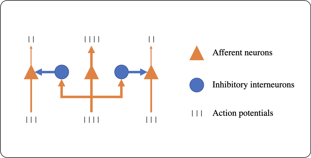
(a) Lateral inhibition process

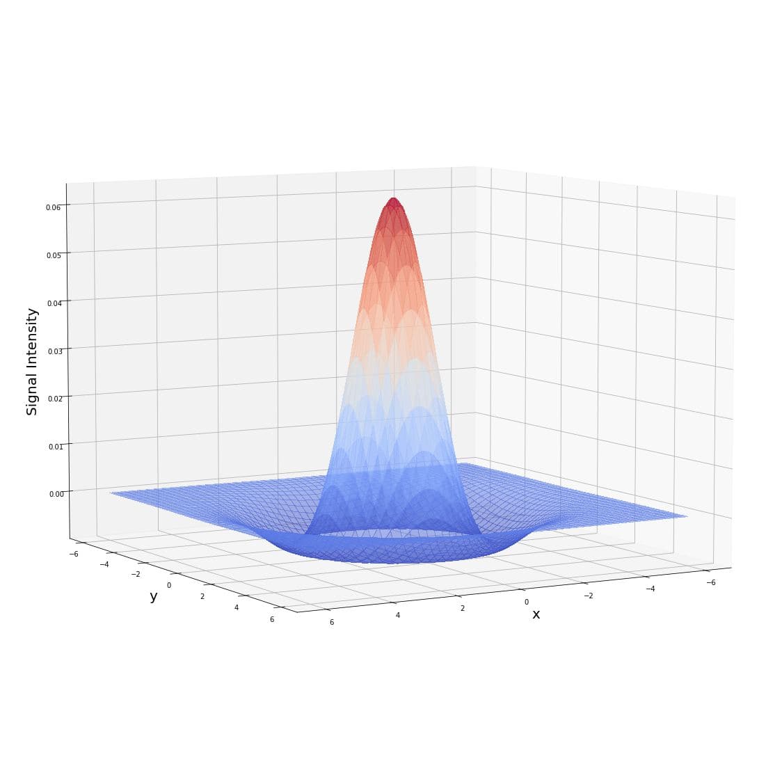
(b) Mexican-hat like distribution

Figure 1: In figure 1(a), the contrast between strong and weak stimuli is amplified after lateral inhibition; In figure 1(b), The Mexican-hat like distribution reflects the effects of LI.

2 Methods

During backpropagation, gradients are generated for all elements the feature map, these then work together to update the corresponding weights. However, previous work [25] showed that not every gradient is critical for training, so the importance of the gradient needs to be measured. In order to achieve this goal, we implement the LI mechanism with Laplacian of Gaussian (LoG) operator in the backpropagation process of ANN, because the LI mechanism makes the signal distributed like a Mexican hat, and the LoG operator functions similarly. The operator assigns a value to each feature gradient as a measure of its importance, and through theoretical intuition and experiments we show that this measure of importance is reasonable and effective. During training based on this metric Gradient Mask is generated to filter out unimportant feature gradients, so that back propagation is performed in a subnet.

2.1 Gradient Mask

For convolutional layer $l$ with feature maps of width $u$ and height $v$, we divide all the feature maps into $K$ sets evenly. For each set, in order to reduce the computational complexity, the gradients at the same coordinate are composed into a vector called minicolumn, which constitutes a fundamental computational unit of the cerebral cortex [45, 44, 46, 32, 7, 7]. We denote the minicolumn on the coordinates $(i,j)$ of the $k$-th set as $M_{ij}^{l}(k)$. We calculate its $l_{2}$ norm $||M_{ij}^{l}(k)||_{2}$ to represent the magnitude of the gradients in this minicolumn.

Then for each $k$ we apply the $LoG$ operator to the matrix composed of $||M_{ij}^{l}(k)||_{2}$ for all $0\leq i\leq u,0\leq j\leq v$. This process is done with $LoG$ convolution kernel,

$$LoG(x,y) =\frac{\partial^{2}G_{\sigma}(x,y)}{\partial x^{2}}+\frac{\partial^{2}G_{\sigma}(x,y)}{\partial y^{2}}$$ (1)

$$=-\frac{1}{\pi\sigma^{4}}[1-\frac{x^{2}+y^{2}}{2\sigma^{2}}]e^{-\frac{x^{2}+y^{2}}{2\sigma^{2}}}$$ (2)

where $(x,y)$ refers to the coordinates of the $LoG$ convolution kernel and $G_{\sigma}(x,y)$ is the Gaussian convolution with standard deviation $\sigma$. Let $\delta^{l}_{ij}(k)$ denote the result of the $LoG$ convolution on the corresponding part.

By setting the threshold to $\epsilon$, we can define the set of coordinates on which the gradient is not important,

$$A^{l}(k)=\{(i,j):|\delta^{l}_{ij}(k)|<\epsilon\}$$ (3)

Therefor we can generate the Gradient Mask: $Mask^{l}(k)=[a_{ij}]_{u\times v}$, where

$$a_{ij}=\left\{\begin{array}[]{rcl}0&&,{(i,j)\in A^{l}(k)}\\ 1&&,{(i,j)\not\in A^{l}(k)}\\ \end{array}\right.$$ (6)

Since gradient mask $Mask^{l}(k)$ corresponds to the $k$-th set of the feature maps, the filters corresponding to this set of feature maps share the same mask $Mask^{l}(k)$. During backpropagation, each gradient passes through the gradient mask, i.e. multiplied by the mask in an element-wise fashion, and then continues to propagate. Let $L$ denote the loss, the gradient of the weight $w_{mn}^{l}$ on a filter may be written as

$$\frac{\partial L}{\partial w^{l}_{mn}} =\frac{\partial L}{\partial a^{l}_{11}}\frac{\partial a^{l}_{11}}{\partial w^{l}_{mn}}+\dots+\frac{\partial L}{\partial a^{l}_{NN}}\frac{\partial a^{l}_{NN}}{\partial w^{l}_{mn}}$$ (7)

$$=\underbrace{\sum_{(i,j)\in A^{l}}\frac{\partial L}{\partial a^{l}_{ij}}\frac{\partial a^{l}_{ij}}{\partial w^{l}_{mn}}}_{inhibited~{}part}+\underbrace{\sum_{(i^{\prime},j^{\prime})\not\in A^{l}}\frac{\partial L}{\partial a^{l}_{i^{\prime}j^{\prime}}}\frac{\partial a^{l}_{i^{\prime}j^{\prime}}}{\partial w^{l}_{mn}}}_{important~{}part}$$ (8)

$$=0+\underbrace{\sum_{(i^{\prime},j^{\prime})\not\in A^{l}}\frac{\partial L}{\partial a^{l}_{i^{\prime}j^{\prime}}}\frac{\partial a^{l}_{i^{\prime}j^{\prime}}}{\partial w^{l}_{mn}}}_{important~{}part}$$ (9)

The unimportant feature gradients are set to 0; therefore, the weight only changes in the direction indicated by the important feature gradients, which helps to denoise the feature information retained in the weight [2], improving robustness of the network. This is illustrated in experiments which test the performance of our model against adversarial attacks 3.3.2. The denoising effect is also illustrated in the GSNR (Gradient Signal to Noise Ratio) (see Section 3.3.3).

With gradients masked during back-propagation, given the same accuracy, one can intuitively understand that most features are packed into a smaller subset of useful weights. This is illustrated in the network loss of accuracy during pruning, as discussed in section 3.3.1. Figure 2 describes how Gradient Mask is generated and affects the backpropagation. Algorithm 1 illustrates the entire process of our method.

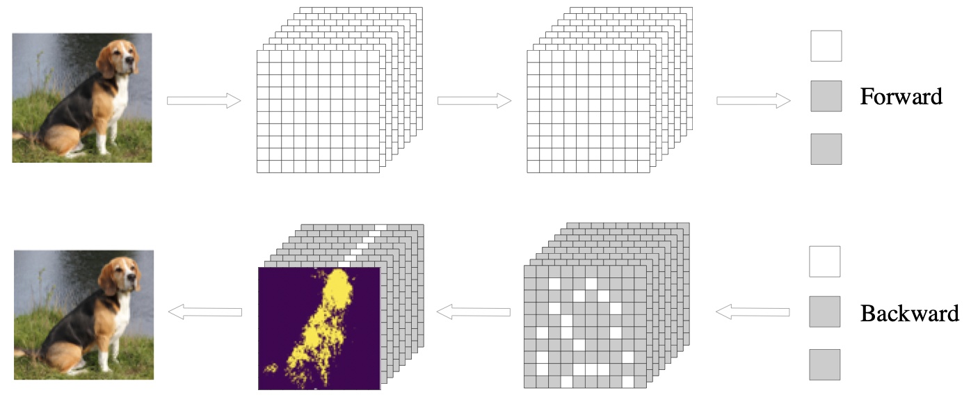
Figure 2: Lateral Inhibition in neural networks. The white square represents the activated neuron while the gray square is inhibited, and the gradient is only flowing through the activated neurons.

2.2 Gradient Flux Sensitivity

In this section, we provide the theoretical intuition of the Gradient Mask, which is to show the rationality of using $\delta^{l}_{ij}$ to measure the importance of the feature gradients.

In backpropagation, as shown in equation (5), a weight gradient can be decomposed into multiple terms, and each term corresponds to a coordinate on the feature map. In order to express how significant a point on the feature map is to a weight gradient $g^{l}_{mn}$, we calculate its laplacian along the coordinates $(i,j)$ on the feature map:

$$\Delta g_{mn}^{l}=\frac{\partial^{2}g_{mn}^{l}}{\partial i^{2}}+\frac{\partial^{2}g_{mn}^{l}}{\partial j^{2}}$$ (10)

Physically speaking, it is the divergence of the change of the gradient $g^{l}_{mn}$ in space, and its absolute value indicates to what extent the point $(i,j)$ is the ”source” (positive or negative source) of the gradient $g^{l}_{mn}$ [23]. A larger source means that it is more significant and critical for the gradient $g^{l}_{mn}$. We define it as Gradient Flux Sensitivity $s^{l}_{mn}=|\Delta g_{mn}^{l}|$.

Let $\overline{\frac{\partial L}{\partial a^{l}_{ij}}}$ be the feature gradient after Gaussian smoothing. So that the gradient flux sensitivity can be rewritten as follows:

$$s_{mn}^{l} =\left|\Delta\sum_{i,j}(\overline{\frac{\partial L}{\partial a^{l}_{ij}}}\frac{\partial a^{l}_{ij}}{\partial w^{l}_{mn}})\right|$$ (11)

$$=\frac{\partial a^{l}_{ij}}{\partial w^{l}_{mn}}\left|\Delta\overline{\frac{\partial L}{\partial a^{l}_{ij}}}\right|$$ (12)

The coefficient $\frac{\partial a^{l}_{ij}}{\partial w^{l}_{mn}}$ is the derivative of the activation function given the input of the neuron, which can be regarded as a constant, and is non-negative since ReLU is the activation function. So the element of the Gradient Mask $\delta^{l}_{ij}=\left|\Delta\overline{\frac{\partial L}{\partial a^{l}_{ij}}}\right|$ is positively related to $s_{mn}^{l}$, therefore $\delta^{l}_{ij}$ can measure the importance of feature gradients to a weight gradient.

Algorithm 1 Generation of Gradient Masks for one sample in layer $l$

1:Tensor of gradients in layer $l$, Quantile, Sigma, Kernel size, Number of channels, Number of sets.

2:Initialize $G^{l}$ = Tensor of gradients in layer $l$, $q$ = Quantile, $\sigma$ = Sigma, $s$ = Kernel size, $C$ = Number of channels , $K$ = Number of sets. Let $l_{c}$ be the $c$-th feature map of layer $l$,

$$G^{l}=[\frac{\partial{L}}{\partial{a_{ij}^{l_{c}}}}]_{C\times u\times v}$$ (13)

3:Divide gradients into minicolumns:

$$M^{l}_{ij}(k)=[\frac{\partial{L}}{\partial{a_{ij}^{l_{c^{\prime}}}}}]_{\frac{C}{K}\times 1}$$ (14)

and compute $l_{2}$ norm of each minicolumn: $||M^{l}_{i,j}(k)||_{2}$ to get $K$ matrices:

$$D^{l}(k)=[||M^{l}_{ij}(k)||_{2}]_{u\times v},$$ (15)

4:Perform $LoG$ convolution on each matrix $D^{l}(k)$ with given parameters $\sigma$ and $s$:

$$\delta_{ij}^{l}(k)=LoG_{\sigma,s}(D^{l}(k))$$ (16)

5:Calculate threshold value $Q_{k}^{l}$ with given parameter quantile $q$:

$$Q^{l}_{k}=Threshold({[\delta_{ij}^{l}(k)]_{u\times v},q)}$$ (17)

6:Generate Gradient Masks:

$$Mask^{l}(k)=[\mathbb{I}_{|\delta^{l}_{ij}(k)|>Q_{k}}]_{u\times v}$$ (18)

7:Update the gradients on each feature map $c$ with the Gradient Mask:

$$\overline{G_{c}^{l}}=[\frac{\partial{L}}{\partial{a_{ij}^{l_{c}}}}]_{u\times v}\circ Mask^{l}(k)|_{k\in\{k|l_{c}\in set(k)\}}$$ (19)

8:Continue backpropagation with $\overline{G^{l}}=[\overline{G^{l}_{c}}]_{C\times 1}$.

3 Experiments

Training with Gradient Mask, our model achieved higher accuracy on ImageNet [12] and CIFAR-100 [24] datasets. And In order to visualize the effect of the Gradient Mask method, we use the LoG operator to generate saliency maps, and compare them with the saliency maps generated by other methods like Grad-CAM[40], verifying that this method is able to more accurately capture key features.

The network trained with Gradient Mask has also improved in robustness and generalization ability, which comes from the accumulation of signals and the inhibition of noise:

• In terms of signal, the pruning experiment shows that the model can be pruned more while maintaining accuracy, indicating that the key gradients are indeed packed into a sparser sub-network;

• In terms of noise, adversarial experiments show that the noise gradients are less learned by the model.

• Furthermore, we quantitatively demonstrate the relative enhancement of the signal and the reduction of the noise by calculating the Gradient Signal to Noise Ratio (GSNR) [28].

Finally, applying Lateral Inhibition, we propose a new data enhancement scheme that can detect and blur unimportant parts of the images in real time.

3.1 Training with Gradient Mask

To fairly compare the performance of the original network and the network trained with Gradient Mask, we use ResNet[19] as the experimental framework and apply the same hyperparameters and data enhancement strategy. In order to generate the Gradient Mask, we set additional hyperparameters $\sigma=11$, $K=16$, and the quantile(inhibition rate) at $50\%$. We apply Gradient Mask on the output layer of every bottleneck except the last two bottlenecks, which contain rich semantic information, and too much inhibition would lead to degradation of network performance. Although using the same learning rate as the original network is not the optimal choice for the Gradient Masked network, as the latter only updates the weights in its sub-network, but in order to make a fair comparison, we use the same hyperparameters as the original network. We conducted classification experiments on ImageNet (with 8 Tesla V100 GPUs) and CIFAR-100 (with 1 Tesla V100 GPU) respectively, and the experiments showe that using Gradient Mask improves classification accuracy. Table 1 shows the result of ResNet with/without gradient masks in the two datasets.

Model	CIFAR-100	ImageNet
Normal ResNet-18/50	78.2	75.5
Masked ResNet-18/50	80.26	76.01

Table 1: The top-1 accuracy (%) of ResNet-18 with/without masks on CIFAR-100 and ResNet-50 with/without mask on ImageNet

In order to investigate whether LI and minicolumns are crucial for Gradient Mask to work, two experiments are conducted: in the first experiment, after slicing the pixel channels into minicolumns, we perform an $l_{2}$ norm operation on each minicolumn, and we took the quantile directly from the norm results to decide which minicolumns should be inhibited/activated (without LI); in the second experiment, we do not aggregate neurons as minicolumn, we take the absolute value of each pixel on each feature map, and then perform $LoG$ on the feature map (without minicolumn).

Model	Masked ResNet-18	Without LI	Without Minicolumn
Accuracy	80.26	75.86	78.97

Table 2: The top-1 accuracy (%) of ResNet-18 with and without LI and Minicolumn on CIFAR-100

We use ResNet-18 and the same hyperparameters to conduct the experiment in CIFAR-100. The results are shown in Table 2 and Figure 3, we show that $LoG$ is crucial for the generation of Gradient Mask - Without LI reduces the accuracy significantly. The accuracy of Without Minicolumn is lower than Masked ResNet-18, and its training speed is 3 times slower than Masked ResNet-18 (more masks need to be generated).

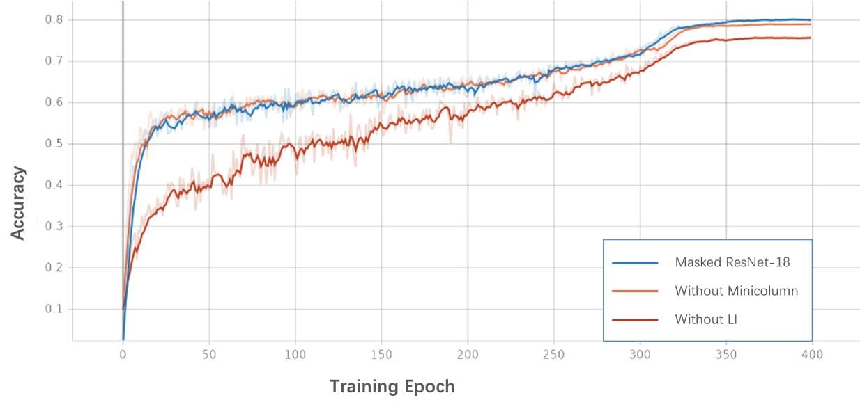
Figure 3: Training with and without LoG and Minicolumn in CIFAR-100 dataset.

3.2 Saliency Map

Saliency map highlights portion of the image that contributes to a classification decision, hence it is an effective tool for the interpretation of convolutional neural networks (CNN). In recent years, various saliency detection methods have been proposed: Guided Backpropagation(GBP) [43], Class Activation Mapping(CAM)[52], Grad-CAM[40], Grad-CAM++[9] and so on. Although some saliency detection methods [43] are able to generate the saliency map, they are independent of the model and data generation process, and may not best explain the relationship between the inputs and outputs of the model during learning or to debug the model [1].

We used the LI method on a CNN to generate better saliency maps, which we named as LI-Map. Additional experiments were conducted to show that the saliency map generated with LI pass the Cascading Randomization test [1] (See Appendix A), confirming that the generated saliency map is helpful for interpretability of the network.

For every activation layer $A^{l}$, we apply step 1-3 from Algorithm 1 to get $\delta^{l}$. Notice that: 1) Replace loss $L$ with $P$, where $P$ is the prediction of interest; 2) Set $K=1$, i.e. each pixel channel can be seen as one minicolumn. Then resize $\delta^{l}$ from $u\times v$ to $H\times W$, where $H$ and $W$ are the height and width of the input image:

$$\delta^{l}=LoG_{\sigma,s}(D^{l})$$ (20)

$$\delta^{l}\in\mathbb{R}^{u\times v}\rightarrow\delta^{l}\in\mathbb{R}^{H\times W}$$ (21)

Finally, in order to combine information from each layer, we sum the $\delta^{l}$ of all activation layers to get the saliency map $F$:

$$F=\sum_{l=1}^{t}\delta^{l},\quad l\in[1,t]$$ (22)

where $t$ is the number of activation layers. Figure 4 shows our results compared with Grad-CAM. We can see that the saliency maps generated by LI-Map are more accurately focused on the target objects.

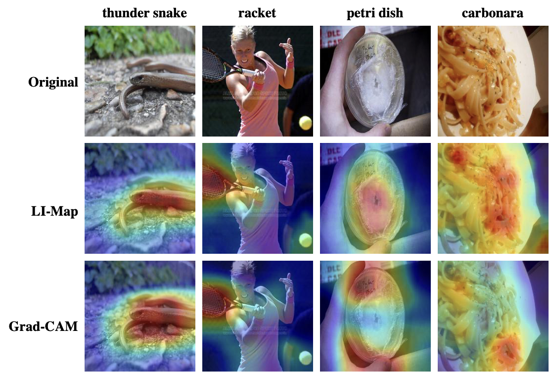
Figure 4: Saliency maps generated by LI-Map and Grad-CAM. Note that the saliency maps generated by LI-Map are more accurately focused on the target objects.

With the aim of quantitatively comparing the object detection ability of various saliency map methods, we propose a measure based on Intersection over Union (IoU) scores. We select 15% of pixels with the largest F values (F is calculated by Equation 22) in the saliency map generated by the different methods as the region of interest. The smallest and largest coordinate points of these pixels are used to form a rectangular bounding box and the IoU score is calculated with the real bounding box where the target is located. As shown in Table 3, we verify the superiority of our method on the PASCAL VOC 2007 [15] and ImageNet datasets.

Dataset	Grad-CAM	Grad-CAM++	LI-Map
PASCAL VOC 2007	0.44	0.45	0.5
ImageNet	0.46	0.46	0.49

Table 3: The IoU results on PASCAL VOC 2007 and ImageNet

In order to further understand the impact of using Gradient Mask, we visualize different saliency maps trained with no mask, up to one mask per image, see Appendix B.

3.3 Robustness and Generalization performance

3.3.1 Network Pruning

To confirm that the network trained with Gradient Mask has the ability to intensively learn features into a sparser subnet, we trained a GM-ResNet-50 using Gradient Mask, pruned it with L1 (we pruned a certain percentage of the weights with the smallest absolute value between layers or globally to observe the performance of the network) and compared it with a normally trained ResNet-50. As shown in Figure 5, the network with Gradient Mask has better performance after pruning.

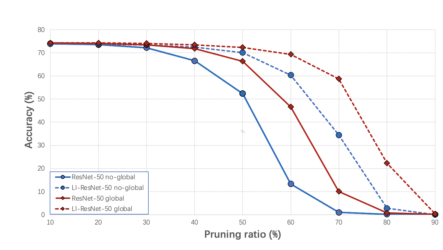
Figure 5: The LI-based network has better performance after pruning

3.3.2 Adversarial Attack

In order to test the robustness of the network trained with Gradient Mask, we conducted adversarial attacks on it. We apply Fast Gradient Sign Attack (FGSM) [17] on both models (GM-ResNet-50 and normal ResNet-50). The dataset comprises of images from ImageNet validation set that can be correctly predicted by both models. As shown in Figure 6, model trained with Gradient Mask is more robust against adversarial attacks.

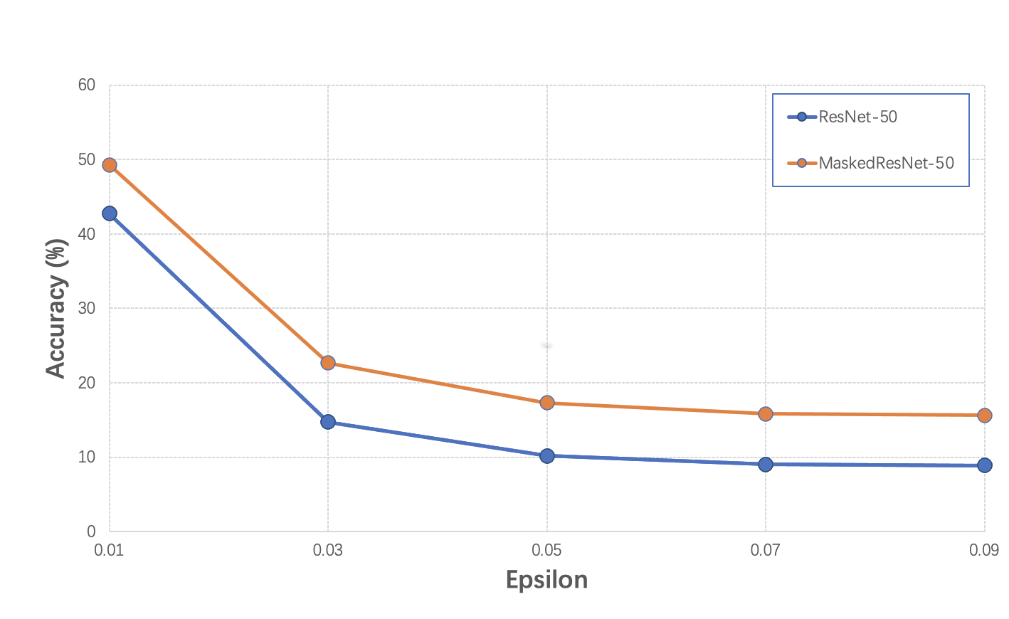
Figure 6: The LI-based network has better capabilities against adversarial attacks compared with ordinary networks.

3.3.3 Gradient Mask leads to better GSNR

In order to test the performance of Gradient Mask in filtering noise gradient, we use the Gradient Signal to Noise Ratio (GSNR) [28] that has been shown to quantify network generalizability. The GSNR of a model parameter $\theta_{j}$ is defined as:

$$r\left(\theta_{j}\right):=\frac{\tilde{\mathbf{g}}^{2}\left(\theta_{j}\right)}{\rho^{2}\left(\theta_{j}\right)}$$

where $\tilde{\mathbf{g}}\left(\theta_{j}\right)$, $\rho\left(\theta_{j}\right)$ are mean and variance of $\theta_{j}$ in the iteration, respectively. In our experiment, we compare the GSNR of convolutional layers between normal training and training with Gradient Mask in CIFAR-10 [24]. Figure LABEL:gsnr shows that Gradient Mask can improve GSNR of the model during training, indicating training with Gradient Mask can improve the generalization of the network.

3.4 Data Enhancement

Data enhancement is an effective method to improve the generalization and robustness of a neural network. Previous works [51, 49] demonstrated that context and background will greatly affect the performance of the network and the network can easily overfit to the background during training. As Section 3.2 shown, LI can help to locate the target of interest in real time, so that we can insert noise in the non-target area (background or other objects) for data enhancement.

Since no annotation was found for the ImageNet validation set, we selected 100,000 images with bounding box from 1.28 million images as the validation set, and retrained the ResNet-50 on the rest 1.18 million images. Figure 8 shows the examples from the validation dataset, in which sigma is the blur ratio. Based on the retrained ResNet-50, we continued to train the model using data augmentation for 30 epochs, tested it on 100,000 images with bounding box and Gaussian blur, and compared it with the original pre-trained model. The algorithm is described in Algorithm 2. Examples of enhanced images are shown in Figure 9, we can observe that the irrelevant information of the target object in the image is well covered.

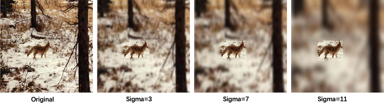
Figure 8: Examples from validation dataset

Algorithm 2 Data Enhancement with Gradient Mask

1:Input tensor with shape $N\times 3\times H\times W$, Quantile, Sigma, Kernel size, Set of activation layers

2:Output tensor with shape $N\times 3\times H\times W$.

3:Initialize $I$ = Input tensor, $q$ = Quantile, $\sigma$ = Sigma, $s$ = Kernel size, $K$ = Number of Sets = 1, $A=\{A^{1},A^{2},\ldots,A^{t}\}$ = Set of activation layers.

4:For every activation layer $A^{l}$, $1\leq l\leq t$ in $A$, apply steps 1-3 in algorithm 1. Then Use linear interpolation to scale $\delta^{l}$ to input size $(H,W)$.

$$\delta^{l} =LoG_{\sigma,s}(D^{l})$$ (23)

$$\delta^{l}\in\mathbb{R}^{N\times 1\times u\times v} \rightarrow\delta^{l}\in\mathbb{R}^{N\times 1\times H\times W}$$ (24)

5:Summary all $\delta^{l}$ on second dimession:

$$F=\sum_{l=1}^{t}\delta^{l},\quad F\in\mathbb{R}^{N\times 1\times H\times W}$$ (25)

6:Calculate threshold value $Q$ with given parameter quantile $q$:

$$Q=Threshold({[F_{ij}]_{H\times W},q)},\quad Q\in\mathbb{R}^{N}$$ (26)

7:Generate input Mask for every sample:

$$Mask=[\mathbb{I}_{|F_{ij}|>Q}]_{H\times W},Mask\in\{0,1\}^{N\times 1\times H\times W}$$ (27)

8:Random sampling $r\%$ images from the input, then apply Gaussian blur on their inhibited areas (i.e where mask[i,j]= 0) to obtain the enhanced image.

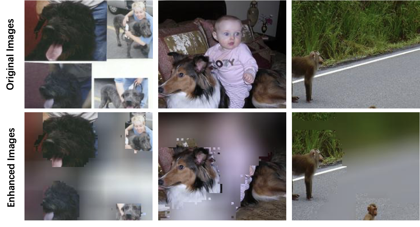
Figure 9: Generation of enhanced images with lateral inhibition.

Figure LABEL:enhancement shows the result of ResNet-50 and enhanced ResNet-50 on the validation set with different blur ratio applied to their ”background”. It can be seen that the data-enhanced network has better robustness in the dataset with blurred background.

4 Conclusion and Discussion

In this work, we propose a novel CNN training technique inspired by biological lateral inhibition - Gradient Mask - for filtering noise gradients during the backpropagation process so as to improve its performance. The experimental results show that, accuracy of the original CNN architecture, after pruning, and under adversarial attacks, improves. CNN trained with Gradient Mask also generates better saliency maps, which is used for data enhancement which achieves better network interpretability. Furthermore, we provide an analytical explanation for these improvements based on a new criterion for gradient quality: the gradient flux sensitivity.

For future work, we would consider making some of the hyper-parameters, such as the inhibition rate of each layer/bottleneck, $\sigma$ in LoG, the number of groups of channel division, learnable. Gradient Mask applies the notion of LI during back-propagation. How would one implement LI in the forward-propagation, and what purpose would it serve? With the recent advances made by Transformers in CV and NLP [47, 13, 6, 14, 53, 36], and its potential to unify different neural network architectures [36], and to form minicolumn naturally, one may contemplate how LI maybe introduce to the transformer.

References

- [1] Julius Adebayo, Justin Gilmer, Michael Muelly, Ian Goodfellow, Moritz Hardt, and Been Kim. Sanity checks for saliency maps. arXiv preprint arXiv:1810.03292, 2018.
- [2] Zeyuan Allen-Zhu and Yuanzhi Li. Feature purification: How adversarial training performs robust deep learning. arXiv preprint arXiv:2005.10190, 2020.
- [3] Shun-ichi Amari. Dynamics of pattern formation in lateral-inhibition type neural fields. Biological cybernetics, 27(2):77–87, 1977.
- [4] Andrea Banino, Caswell Barry, Benigno Uria, Charles Blundell, Timothy Lillicrap, Piotr Mirowski, Alexander Pritzel, Martin J Chadwick, Thomas Degris, Joseph Modayil, et al. Vector-based navigation using grid-like representations in artificial agents. Nature, 557(7705):429–433, 2018.
- [5] Francesco P Battaglia and Alessandro Treves. Attractor neural networks storing multiple space representations: a model for hippocampal place fields. Physical Review E, 58(6):7738, 1998.
- [6] Tom B Brown, Benjamin Mann, Nick Ryder, Melanie Subbiah, Jared Kaplan, Prafulla Dhariwal, Arvind Neelakantan, Pranav Shyam, Girish Sastry, Amanda Askell, et al. Language models are few-shot learners. arXiv preprint arXiv:2005.14165, 2020.
- [7] Daniel P Buxhoeveden and Manuel F Casanova. The minicolumn and evolution of the brain. Brain, Behavior and Evolution, 60(3):125–151, 2002.
- [8] Yongqiang Cao, Yang Chen, and Deepak Khosla. Spiking deep convolutional neural networks for energy-efficient object recognition. International Journal of Computer Vision, 113(1):54–66, 2015.
- [9] Aditya Chattopadhay, Anirban Sarkar, Prantik Howlader, and Vineeth N Balasubramanian. Grad-cam++: Generalized gradient-based visual explanations for deep convolutional networks. In 2018 IEEE Winter Conference on Applications of Computer Vision (WACV), pages 839–847. IEEE, 2018.
- [10] Ting Chen, Simon Kornblith, Mohammad Norouzi, and Geoffrey Hinton. A simple framework for contrastive learning of visual representations. In International conference on machine learning, pages 1597–1607. PMLR, 2020.
- [11] Steven J Cooper. Donald o. hebb’s synapse and learning rule: a history and commentary. Neuroscience & Biobehavioral Reviews, 28(8):851–874, 2005.
- [12] Jia Deng, Wei Dong, Richard Socher, Li-Jia Li, Kai Li, and Li Fei-Fei. Imagenet: A large-scale hierarchical image database. In 2009 IEEE conference on computer vision and pattern recognition, pages 248–255. Ieee, 2009.
- [13] Jacob Devlin, Ming-Wei Chang, Kenton Lee, and Kristina Toutanova. Bert: Pre-training of deep bidirectional transformers for language understanding. arXiv preprint arXiv:1810.04805, 2018.
- [14] Alexey Dosovitskiy, Lucas Beyer, Alexander Kolesnikov, Dirk Weissenborn, Xiaohua Zhai, Thomas Unterthiner, Mostafa Dehghani, Matthias Minderer, Georg Heigold, Sylvain Gelly, et al. An image is worth 16x16 words: Transformers for image recognition at scale. arXiv preprint arXiv:2010.11929, 2020.
- [15] M. Everingham, L. Van Gool, C. K. I. Williams, J. Winn, and A. Zisserman. The PASCAL Visual Object Classes Challenge 2007 (VOC2007) Results. http://www.pascal-network.org/challenges/VOC/voc2007/workshop/index.html.
- [16] Gabriel Goh, Nick Cammarata, Chelsea Voss, Shan Carter, Michael Petrov, Ludwig Schubert, Alec Radford, and Chris Olah. Multimodal neurons in artificial neural networks. Distill, 6(3):e30, 2021.
- [17] Ian J Goodfellow, Jonathon Shlens, and Christian Szegedy. Explaining and harnessing adversarial examples. arXiv preprint arXiv:1412.6572, 2014.
- [18] Kaiming He, Haoqi Fan, Yuxin Wu, Saining Xie, and Ross Girshick. Momentum contrast for unsupervised visual representation learning. In Proceedings of the IEEE/CVF Conference on Computer Vision and Pattern Recognition, pages 9729–9738, 2020.
- [19] Kaiming He, Xiangyu Zhang, Shaoqing Ren, and Jian Sun. Deep residual learning for image recognition. In Proceedings of the IEEE conference on computer vision and pattern recognition, pages 770–778, 2016.
- [20] Olivier Henaff. Data-efficient image recognition with contrastive predictive coding. In International Conference on Machine Learning, pages 4182–4192. PMLR, 2020.
- [21] Geoffrey E Hinton, Alex Krizhevsky, and Sida D Wang. Transforming auto-encoders. In International conference on artificial neural networks, pages 44–51. Springer, 2011.
- [22] John J Hopfield. Neural networks and physical systems with emergent collective computational abilities. Proceedings of the national academy of sciences, 79(8):2554–2558, 1982.
- [23] Victor J Katz. The history of stokes’ theorem. Mathematics Magazine, 52(3):146–156, 1979.
- [24] Alex Krizhevsky, Geoffrey Hinton, et al. Learning multiple layers of features from tiny images. 2009.
- [25] Janice Lan, Rosanne Liu, Hattie Zhou, and Jason Yosinski. Lca: Loss change allocation for neural network training. arXiv preprint arXiv:1909.01440, 2019.
- [26] Yann LeCun, Bernhard Boser, John S Denker, Donnie Henderson, Richard E Howard, Wayne Hubbard, and Lawrence D Jackel. Backpropagation applied to handwritten zip code recognition. Neural computation, 1(4):541–551, 1989.
- [27] Timothy P Lillicrap, Adam Santoro, Luke Marris, Colin J Akerman, and Geoffrey Hinton. Backpropagation and the brain. Nature Reviews Neuroscience, 21(6):335–346, 2020.
- [28] Jinlong Liu, Guoqing Jiang, Yunzhi Bai, Ting Chen, and Huayan Wang. Understanding why neural networks generalize well through gsnr of parameters. arXiv preprint arXiv:2001.07384, 2020.
- [29] William Lotter, Gabriel Kreiman, and David Cox. Deep predictive coding networks for video prediction and unsupervised learning. arXiv preprint arXiv:1605.08104, 2016.
- [30] Warren S McCulloch and Walter Pitts. A logical calculus of the ideas immanent in nervous activity. The bulletin of mathematical biophysics, 5(4):115–133, 1943.
- [31] Kenneth D Miller. Synaptic economics: competition and cooperation in synaptic plasticity. Neuron, 17(3):371–374, 1996.
- [32] Vernon B Mountcastle. The columnar organization of the neocortex. Brain: a journal of neurology, 120(4):701–722, 1997.
- [33] Aaron van den Oord, Yazhe Li, and Oriol Vinyals. Representation learning with contrastive predictive coding. arXiv preprint arXiv:1807.03748, 2018.
- [34] Michael Pfeiffer and Thomas Pfeil. Deep learning with spiking neurons: opportunities and challenges. Frontiers in neuroscience, 12:774, 2018.
- [35] Isabella Pozzi, Sander Bohte, and Pieter Roelfsema. Attention-gated brain propagation: How the brain can implement reward-based error backpropagation. Advances in Neural Information Processing Systems, 33, 2020.
- [36] Alec Radford, Jong Wook Kim, Chris Hallacy, Aditya Ramesh, Gabriel Goh, Sandhini Agarwal, Girish Sastry, Amanda Askell, Pamela Mishkin, Jack Clark, et al. Learning transferable visual models from natural language supervision. arXiv preprint arXiv:2103.00020, 2021.
- [37] Rajesh PN Rao and Dana H Ballard. Predictive coding in the visual cortex: a functional interpretation of some extra-classical receptive-field effects. Nature neuroscience, 2(1):79–87, 1999.
- [38] Frank Rosenblatt. The perceptron: a probabilistic model for information storage and organization in the brain. Psychological review, 65(6):386, 1958.
- [39] Sara Sabour, Nicholas Frosst, and Geoffrey E Hinton. Dynamic routing between capsules. arXiv preprint arXiv:1710.09829, 2017.
- [40] Ramprasaath R Selvaraju, Michael Cogswell, Abhishek Das, Ramakrishna Vedantam, Devi Parikh, and Dhruv Batra. Grad-cam: Visual explanations from deep networks via gradient-based localization. In Proceedings of the IEEE international conference on computer vision, pages 618–626, 2017.
- [41] Abhronil Sengupta, Yuting Ye, Robert Wang, Chiao Liu, and Kaushik Roy. Going deeper in spiking neural networks: Vgg and residual architectures. Frontiers in neuroscience, 13:95, 2019.
- [42] Yoko Shoji-Kasai, Hiroshi Ageta, Yoshihisa Hasegawa, Kunihiro Tsuchida, Hiromu Sugino, and Kaoru Inokuchi. Activin increases the number of synaptic contacts and the length of dendritic spine necks by modulating spinal actin dynamics. Journal of Cell Science, 120(21):3830–3837, 2007.
- [43] Jost Tobias Springenberg, Alexey Dosovitskiy, Thomas Brox, and Martin Riedmiller. Striving for simplicity: The all convolutional net. arXiv preprint arXiv:1412.6806, 2014.
- [44] Nicholas V Swindale. Is the cerebral cortex modular? Trends in Neurosciences, 13(12):487–492, 1990.
- [45] J Szentagothai. The ‘module-concept’in cerebral cortex architecture. Brain research, 95(2-3):475–496, 1975.
- [46] Gary W Van Hoesen and Ana Solodkin. Some modular features of temporal cortex in humans as revealed by pathological changes in alzheimer’s disease. Cerebral Cortex, 3(5):465–475, 1993.
- [47] Ashish Vaswani, Noam Shazeer, Niki Parmar, Jakob Uszkoreit, Llion Jones, Aidan N Gomez, Lukasz Kaiser, and Illia Polosukhin. Attention is all you need. arXiv preprint arXiv:1706.03762, 2017.
- [48] Haiguang Wen, Kuan Han, Junxing Shi, Yizhen Zhang, Eugenio Culurciello, and Zhongming Liu. Deep predictive coding network for object recognition. In International Conference on Machine Learning, pages 5266–5275. PMLR, 2018.
- [49] Kai Xiao, Logan Engstrom, Andrew Ilyas, and Aleksander Madry. Noise or signal: The role of image backgrounds in object recognition. arXiv preprint arXiv:2006.09994, 2020.
- [50] Muchao Ye, Xiaojiang Peng, Weihao Gan, Wei Wu, and Yu Qiao. Anopcn: Video anomaly detection via deep predictive coding network. In Proceedings of the 27th ACM International Conference on Multimedia, pages 1805–1813, 2019.
- [51] Mengmi Zhang, Claire Tseng, and Gabriel Kreiman. Putting visual object recognition in context. In Proceedings of the IEEE/CVF Conference on Computer Vision and Pattern Recognition, pages 12985–12994, 2020.
- [52] Bolei Zhou, Aditya Khosla, Agata Lapedriza, Aude Oliva, and Antonio Torralba. Learning deep features for discriminative localization. In Proceedings of the IEEE conference on computer vision and pattern recognition, pages 2921–2929, 2016.
- [53] Xizhou Zhu, Weijie Su, Lewei Lu, Bin Li, Xiaogang Wang, and Jifeng Dai. Deformable detr: Deformable transformers for end-to-end object detection. arXiv preprint arXiv:2010.04159, 2020.