Cavity induced many-body localization

Abstract

In this manuscript, we explore the feasibility of achieving many-body localization in the context of cavity quantum electrodynamics at strong coupling. Working with a spinless electronic Hubbard chain sitting coupled to a single-mode cavity, we show that the global coupling between electrons and photons – which generally would be expected to delocalize the fermionic excitations – can instead favor the appearance of localization. This is supported by a novel high-frequency expansion that correctly accounts for electron-photon interaction at strong coupling, as well as numerical calculations in both single particle and many-bod regimes. We find evidence that many-body localization may survive strong quantum fluctuations of the photon number by exploring energy dependence, seeing signatures of localization down to photon numbers as small as $n\sim 2$.

I Introduction

With the dramatic advance in coherent control during the past decade COH1 ; COH2 , an increasing set of controllable quantum systems are available, such as ultracold atoms, trapped ions, and superconducting qubits. In these systems, experimentalists can steer the dynamics of the system far away from thermal equilibrium, which has stimulated a surge of interest in non-equilibrium dynamics and phases of quantum matter. Examples include new families of topological phases without equilibrium analogs Rudner2013 ; Roy2016 ; MBLTOPO2 ; Else2016 ; Potter2016 ; Nathan2015 ; Roy2017 ; Titum2016 ; Po2016 ; Potter2017 ; Harper2017 ; Roy2017a ; Po2017 ; Potter2018 ; Reiss2018 ; Kolodrubetz2018 ; Nathan2019 ; Timms2021 ; Long2021 ; Nathan2021 , novel forms of symmetry breaking such as quantum time crystals Khemani2016 ; MBLTOPO3 ; Else2016a ; DFTC3 ; zhang2017observation ; Else2020 ; KhemaniArxiv2019 ; Mi2022 , and long-live prethermal states with non-trivial dynamics RubioAbadal2020 ; Peng2021 ; Beatrez2021 . While in general these systems are fragile and eventually heat to a featureless infinite-temperature state, there is strong evidence that this can be circumvented by mitigating slow resonant heating Bukov2016a ; Weidinger2017 , introducing constraints Turner2018 ; Nandkishore2019 , or adding sufficient disorder to realize many-body localization (MBL) FMBL1 ; FMBL2 ; FMBL3 ; ResonanceMBL .

While MBL is a paradigmatic method for avoiding thermalization, its potential beyond locally interacting models with finite on-site Hilbert space remains to be understood. Recently, we have provided strong numerical evidence that MBL can be robust in the context of cavity quantum electrodynamics (QED), where the local interactions within a system of particles or spins competes against global interactions induced by the cavity MBLCentral1 ; MBLCentral2 ; Ng2021 ; these results are confirmed elsewhere Kubala2021 . These papers hinged on the well-explored case of MBL in the presence of time-periodic (Floquet) drive, which becomes a cavity QED model in the appropriate limit. Extending beyond the Floquet limit involves a high-frequency expansion, whose (asymptotic) convergence rests on the separation of scales between the weak cavity/atom coupling and the large photon energy scale.

Yet the most interesting Floquet phenomenon involves resonant driving, for which no such separation of scales exists. In this paper, we investigate the possibility of achieving MBL in a strongly coupled model of cavity QED. Intuitively, the presence of a global cavity mode will induce all-to-all couplings, which will be detrimental to achieving MBL. However, we find the presence of the cavity mode instead favors localization. We show that this behavior is related to the Floquet phenomenon of coherent destruction of tunneling Grossmann1991 ; Lignier2007 and comment on the role of gauge freedom in determining this limit. We provide numerical evidence of a parameter regime where localization survives to a small photon number $n\sim 2$ where quantization of the cavity photon is clearly relevant. We find a version of the high-frequency expansion that can be used to understand these strongly and resonantly driven systems, which we expect will be extensible to a wider variety of cavity QED systems.

II Setup and model

We are interested in the setup illustrated in Figure 1, in which the electric field of a single-mode photonic cavity is coupled to electrons in a one-dimensional system such as a nanowire. The wire is oriented along the polarization direction of the electric field, such that the electronic polarization of the wire, $P=qd\sum_{j}jn_{j}$ – where $q$ is the charge of the particles and $d$ is the lattice spacing – couples directly to the cavity electric field as $\mathbf{P}\cdot\mathbf{E}$. We assume the wire is much shorter than the waist of the cavity mode, such that the electric field amplitude can be treated as uniform along the length of the wire. If we think of the cavity mode in its semi-classical limit, then the electric field will be $E=E_{0}\cos(\omega t)$ where $\omega$ is the cavity frequency. In the strong coupling limit, this large oscillatory electric field interferes with electronic tunneling, resulting in the phenomenon of coherent destruction of tunneling Grossmann1991 ; Lignier2007 . We will be interested to see how this phenomenon holds up in the quantized photon limit, as well as study the role of electronic interactions in localizing the electrons.

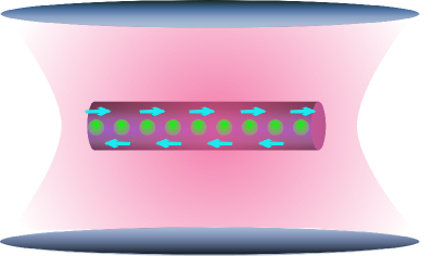
Figure 1: Schematic showing a spinless fermion chain inside a photonic cavity. The electric field polarization of the cavity mode is chosen to be parallel to the length of the chain, such that photons maximally affect the particle motion along the wire.

Modeling this system is surprisingly challenging due to the apparent gauge ambiguity that has been found in cavity QED systems at strong coupling gauge3 . Recently, the gauge ambiguity was found to be induced by truncating the Hilbert space of the matter degrees of freedom gauge ; gauge1 ; gauge2 ; gauge3 . By appropriate truncations, the physical gauge freedom is restored, allowing an unambiguous description of the dynamics within a truncated Hilbert space. While many of these ideas came out of the study of cavity-mediated chemical reactions, where the matter consists of interacting molecules, they can readily be adapted to other systems. Here, we use these techniques to model a single band of spinless fermions in our nanowire. We will refer to these spinless fermions as “electrons” throughout the majority of this paper, but note that none of our results depend on the particular choice of charged fermion.

Let’s begin by considering the most general case, as discussed in gauge , for later generalization. We start with the minimum coupling Hamiltonian for many fermionic degrees of freedom in a single-mode cavity (with $\hbar=1$ throughout) in the Coulomb gauge:

$$H_{C}^{gen}=\sum_{j}\frac{({\bf p_{j}}-q{\bf A({\bf r}_{j}}))^{2}}{2m}+V({\bf r_{j}})+\omega a^{\dagger}a,$$

where ${\bf p}_{j}$ and ${\bf r}_{j}$ are the momentum and position operators of the $j$th particle, $V({\bf r_{j}})$ describes interactions between the particles and their environment (e.g., with the crystal lattice that will give our band structure), and $a^{\dagger}$ is the creation operators of the photon mode with frequency $\omega$. The photon field operator is given by ${\bf A}({\bf r})={\bf f}({\bf r})(ia^{\dagger}-ia)$ with ${\bf f}({\bf r})$ determined by the mode profile. Going into the dipole gauge using the Power-Zienau-Woolley gauge transform $U_{{\rm PZW}}=\exp\big{(}-i\sum_{j}q{\bf r}_{j}\cdot{\bf A}({\bf r}_{j})\big{)}$, we get gauge

$$H_{D}^{gen}= \sum_{j}\left[\frac{p_{j}^{2}}{2m}+V({\bf r_{j}})-\omega q{\bf r}_{j}\cdot{\bf f}({\bf r}_{j})\left(a+a^{\dagger}\right)\right]$$

$$\;\;\;+\omega\left(\sum_{j}q{\bf r}_{j}\cdot{\bf f}({\bf r}_{j})\right)^{2}+\omega a^{\dagger}a,$$

The dipole gauge makes approximating this Hamiltonian much easier, as the electric field has been removed from the kinetic energy term. We are interested in a simple model of one-dimensional spinless fermions on a lattice, for which we choose the disordered single-band Hubbard model. Furthermore, we will assume that the field strength is uniform across the length of the wire, such that $\mathbf{f}(\mathbf{r}_{j})=\mathbf{f}_{0}$ is constant. For a one-dimensional lattice with lattice spacing $d$ and polarization $f$ parallel to the wire, we see that

$$H_{D} =\sum_{j}\Bigg{[}-J\left(c_{j}^{\dagger}c_{j+1}+h.c.\right)+Un_{j}n_{j+1}+V_{j}n_{j}$$

$$\;\;\;\;\;\;-\omega\eta jn_{j}\left(a+a^{\dagger}\right)\Bigg{]}+\omega a^{\dagger}a+\omega\left(\sum_{j}\eta jn_{j}\right)^{2},$$ (1)

in the dipole gauge, where $j$ now sums over sites with particle number $n_{j}=c_{j}^{\dagger}c_{j}$. We have introduced

$$\eta\equiv qdf_{0},$$

as a unitless characterization of the interaction strength between photons and electrons; $\eta\apprge 1$ will correspond to the strong coupling regime. We are interested in quenched disorder with $V_{j}$ drawn independently on each site from a flat distribution: $V_{j}\in[-W,W]$. For this lattice model, the gauge transformation becomes $U_{PZW}=\exp\left[-i\sum_{j}qdjn_{j}f_{0}\left(ia^{\dagger}-ia\right)\right]$. We can use this to return to the Coulomb gauge, for which

$$H_{C} =\sum_{j}\Bigg{[}-J\left(e^{-i\eta\left(ia^{\dagger}-ia\right)}c_{j}^{\dagger}c_{j+1}+h.c.\right)+Un_{j}n_{j+1}$$

$$\;\;\;\;\;\;+V_{j}n_{j}\Bigg{]}+\omega a^{\dagger}a.$$ (2)

The Eqs. (1) and (2) define our main model of interest to be considered throughout this paper. Note that the gauge choice has no physical effect. For example, since they are obtained from unitary transforms of one another, $H_{D}$ and $H_{C}$ are isospectral. For numerical simplicity, the majority of our calculations are done in the dipole gauge, except where stated otherwise.

III High frequency expansion

In order to proceed analytically in understanding the dynamics of the electrons, our goal is to adiabatically eliminate the photons. In previous work on MBL in cavity QED MBLCentral1 , we have done so via a high-frequency expansion, which works when the cavity frequency $\omega$ is much larger than all other microscopic scales in the problem. That work implicitly used the dipole gauge and ignored the polarization-squared term due to weak coupling. Here, however, we are interested in the strong coupling, so these approximations are no longer valid. In this section, we will show how a modified high-frequency expansion (HFE) can be obtained which is valid in the strong coupling limit as well as weak coupling.

To start, we note that in the Coulomb gauge there is in fact a reasonable separation of scales as long as $\omega$ is large. One could proceed to directly eliminate the cavity photon by a canonical transformation similar to Schrieffer-Wolff perturbation theory MBLCentral2 . However, we instead appeal to a useful trick we developed earlier in the context of Floquet drive, namely that the Schrieffer-Wolff transformation can be directly obtained from the effective Hamiltonian of a high-frequency-driven Floquet system Bukov2016 . To use this trick, we start by moving to a rotating frame in which the photon degree of freedom develops time dependence

$$V_{\mathrm{rot}}(t) =\exp(i\omega a^{\dagger}at)$$

$$H_{\mathrm{rot}}(t) =\sum_{j}\Bigg{[}-J\left(e^{-i\eta\left(ia^{\dagger}e^{i\omega t}-iae^{-i\omega t}\right)}c_{j}^{\dagger}c_{j+1}+h.c.\right)$$

$$\;\;\;\;\;\;+Un_{j}n_{j+1}+V_{j}n_{j}\Bigg{]}.$$ (3)

Notice that $H_{\mathrm{rot}}$ is time-periodic with period $T=2\pi/\omega$, enabling the use of Floquet theory to describe this coupled electron-photon system. We can then apply Floquet’s theorem to rewrite the dynamics as HFE1

$$\mathcal{U}_{\mathrm{rot}}(t)=e^{-iK_{\mathrm{eff}}(t)}e^{-iH_{\mathrm{eff}}t}e^{iK_{\mathrm{eff}}(0)}.$$

The effective Hamiltonian can then be approximated by a high-frequency expansion, as detailed in Appendix A. We start by expanding the Hamiltonian as a Fourier series, $H_{\mathrm{rot}}(t)=\sum_{\ell}H^{(\ell)}e^{i\ell\omega t}$. The effective Hamiltonian can be solved perturbatively for large $\omega$ via a high-frequency expansion (HFE) Goldman2014 :

$$H_{\mathrm{eff}}=H^{(0)}+\sum_{\ell>0}\frac{\left[H^{(\ell)},H^{(-\ell)}\right]}{\ell\omega}+\cdots$$

Note that we don’t actually eliminate the photon from our Hilbert space. $H_{\mathrm{eff}}$, as well all of the terms $H^{(\ell)}$, live in the full Hilbert space $\mathcal{H}=\mathcal{H}_{\mathrm{photon}}\otimes\mathcal{H}_{\mathrm{electrons}}$. Instead, one can readily show that the photon number commutes with $H_{\mathrm{eff}}$ at any order of the HFE. Therefore, we can index the effective Hamiltonian by the photon number $n$, such that the complicated photon-electron interactions map to the classical tuning parameter $n$.

At leading (zeroth) order, the effective Hamiltonian is simply given by the time average:

$$H_{\mathrm{eff}}^{0} =\sum_{j}\left[-J_{\mathrm{eff}}\left(c_{j}^{\dagger}c_{j+1}+h.c.\right)+Un_{j}n_{j+1}+V_{j}n_{j}\right]$$

$$J_{\mathrm{eff}} =Je^{-\eta^{2}/2}L_{n}\left(\eta^{2}\right),$$

where $L_{n}(x)$ is the Laguerre polynomial. The first order correction leads to correlated hopping of the form $\left(\sum_{j}c_{j}^{\dagger}c_{j+1}\pm h.c.\right)^{2}$, which are the leading infinite-range integrability-breaking terms that are generally expected to destroy localization. In the appendix, we show that this term vanishes in the limit $\omega\to\infty$ at fixed $\eta$, demonstrating at least asymptotic convergence of the HFE.

III.1 Floquet limit ($n\to\infty$)

In the limit of large photon number, $n\rightarrow\infty$, the effect of cavity photons becomes identical to that of an external classical field, i.e., a Floquet drive. We use the asymptotic formula $L_{n}(x/n)\approx\exp\left[x/(2n)\right]\mathcal{J}_{0}(2\sqrt{x})$ to find

$$J_{\mathrm{eff}}(n,\eta)\approx Je^{-\eta^{2}/2}\mathcal{J}_{0}(2\eta\sqrt{n}),$$

where $\mathcal{J}_{0}$ is the zeroth order Bessel function of the first kind. This is precisely the formula obtained for Floquet driving HFE1 , as expected. It leads to the phenomenon of coherent destruction of tunneling, whereby tunneling is turned off at leading order by tuning to one of the zeros of the Bessel function, e.g., $2\eta\sqrt{n}\approx 2.4$. This idea was used in CIMBL ; CIMBLinherent to suggest drive-induced many-body localization since, in the near absence of tunneling, the disorder should stabilize many-body localization for sufficiently weak interactions.

III.2 Finite photon number

At finite photon number, the effective hopping depends non-trivially on both $\eta$ and $n$. In order to have a well-defined Floquet limit, we clearly need to scale $\eta\sim 1/\sqrt{n}$ at large $n$, but it is less clear what we should do at $n\sim 1$. To motivate the correct scaling, consider the role of weak drive, $\eta\ll 1$, for which we can Taylor expand $J_{\mathrm{eff}}$:

$$\frac{J_{\mathrm{eff}}}{J}=e^{-\eta^{2}/2}L_{n}(\eta^{2})\approx 1-\eta^{2}\left(n+\frac{1}{2}\right).$$

This suggests to rescale $\eta$ as $1/\sqrt{n+1/2}$. Defining the rescaled drive strength

$$\tilde{\eta}\equiv\eta\sqrt{n+1/2},$$

we plot $J_{\mathrm{eff}}(n,\tilde{\eta})$ in Figure 2. At small $\tilde{\eta}$, the different photon numbers match, but they diverge on a scale $\tilde{\eta}\sim n$. The number of zeros – where perfect coherent destruction of tunneling occurs – is equal to $n$, as $L_{n}$ is an $n$th order polynomial with positive real roots. Besides these coherent effects which lead to zeros of the tunneling, there is an overall Gaussian envelope $\exp\left[-\tilde{\eta}^{2}/\left(2n+1\right)\right]$ which suppresses the tunneling at a low photon number for $\eta\apprge 1$. By contrast, $\eta\to 0$ in the limit of large photon number, $n\gg 1$, so we are instead dominated by the oscillatory power-law tails of the Bessel function.

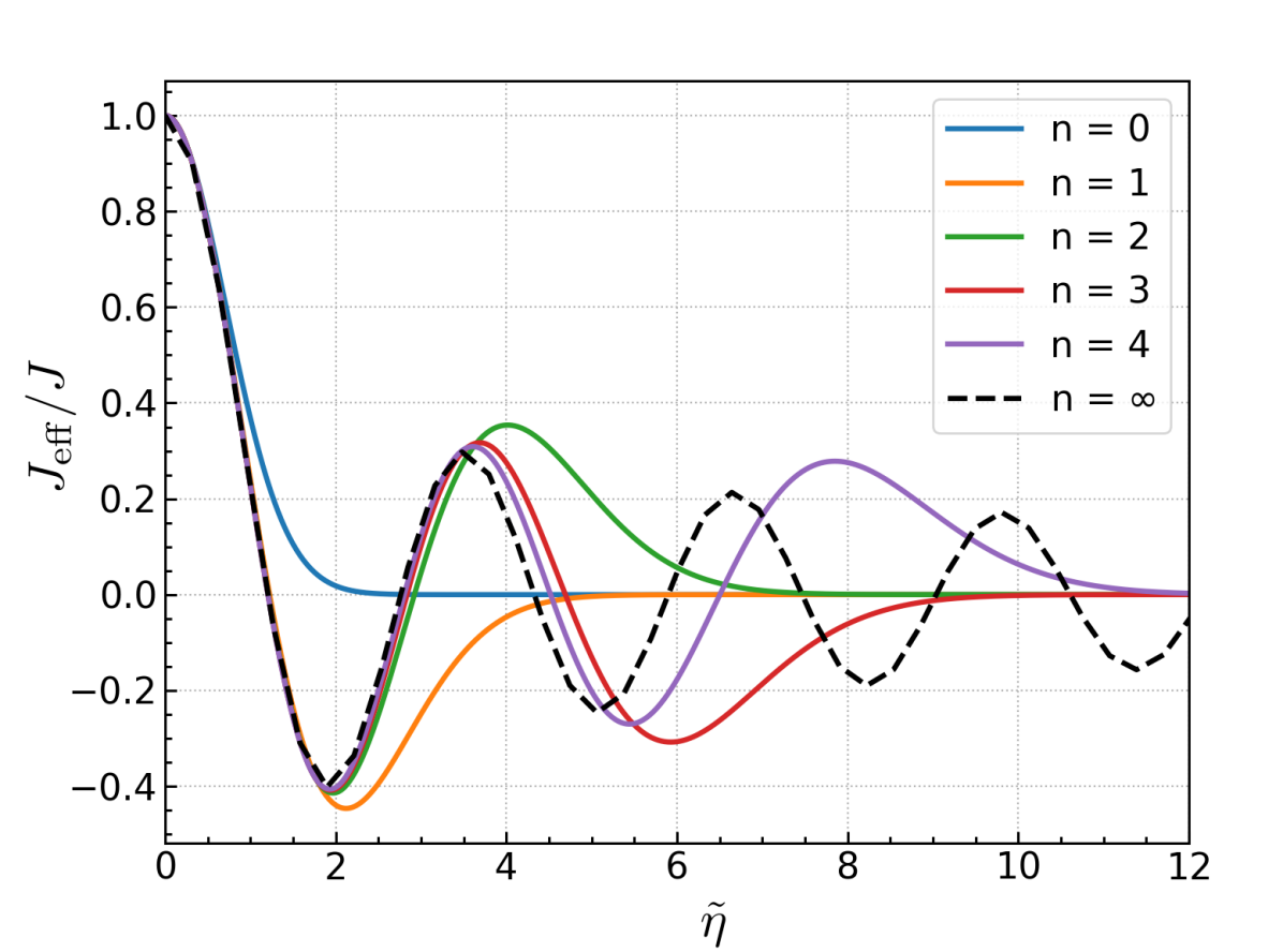
Figure 2: Renormalized coupling strength $J_{\mathrm{eff}}$ as a function of rescaled drive strength $\tilde{\eta}$ for various photon numbers. The limit $n\to\infty$ reproduces Floquet drive, where $J_{\mathrm{eff}}=J\mathcal{J}_{0}(2\tilde{\eta})$.

The second important effect of finite photon number is an infinite range correlated hopping, which is captured at leading order by $H_{\mathrm{eff}}^{1}$. This term is suppressed as $\omega^{-1}$, as expected for a high-frequency expansion. More interestingly, it is also suppressed as $1/n$ within the first order approximation as $n\to\infty$ (see Appendix A), allowing the definition of a Floquet limit where there is clearly no long-range interactions. This is similar to the weakly driven case, in which interactions similarly vanish as $1/(n\omega)$ if the coupling strength is scaled as $1/\sqrt{n}$ (cf. MBLCentral1 ). This suggests that the photon number or coupling strength at which infinite range correlated hopping will induce delocalization scales similarly to the weakly coupled case. The main difference is that the scaled coupling strength $\tilde{\eta}$ has a more interesting dependence, rather than entering directly at low orders in perturbation theory.

Higher order terms in the HFE will give rise to more complicated interactions, as well as local dressing of hopping and interactions due to the commutators of various harmonics with the density-dependent terms in $H_{\mathrm{rot}}^{(0)}$. Terms at order $k$ will be suppressed as $1/(n\omega)^{k}$, so will be negligible in the high frequency and/or large photon number limit.

We now test predictions of the HFE for two cases: the single particle regime (Section IV) and many particle regime (Section V).

IV Single particle localization

If the electron lattice contains a single particle, then the system is integrable and readily solved numerically. Furthermore, the long-range correlated hoppings induced by the cavity mode do not play a role, as terms of the form $c_{j}^{\dagger}c_{j\pm 1}c_{j^{\prime}}^{\dagger}c_{j^{\prime}\pm 1}$ vanish in the single particle sector unless $j=j^{\prime}\pm 1$. Therefore, higher order terms in the HFE simply become longer range hopping: second-nearest neighbor at order 1, third-nearest neighbor at order 2, and so on. Combined with modulation of the nearest neighbor hopping by $J_{\mathrm{eff}}$ (and higher order corrections), we should simply end up with a quasilocal hopping model after integrating out the photon. For our one dimensional model with the chemical potential disorder, such a system will Anderson localize for any finite disorder strength $W>0$.

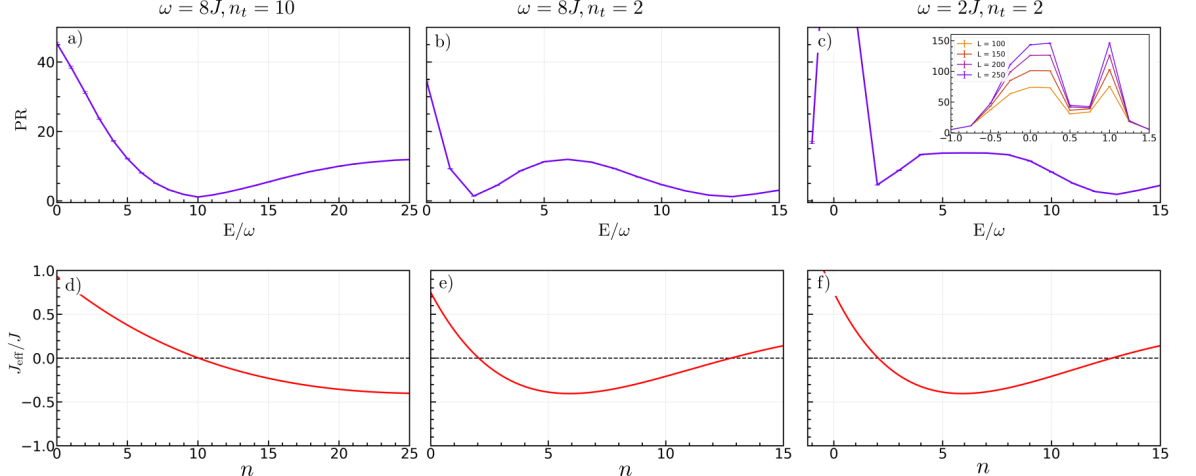
Figure 3: (a-c) Participation ratio (PR) as a function for the single-particle model in 3 regimes: (a) $\omega=8J$ and $n_{t}=10$ ($\eta=0.265$), which approximates the Floquet limit, (b) $\omega=8J$ and $n_{t}=2$ ($\eta=0.765$), where notable deviations exist from the Floquet limit but the high-frequency expansion (HFE) is still useful, and (c) $\omega=2J$ and $n_{t}=2$, where the photon frequency is less than the bandwidth and, therefore, the HFE should not hold. For (a-c), disorder is $W=0.5$ and system size is $L=250$. Results are averaged over disorder realizations and energy in the window $E\pm\omega/2$; error bars are smaller than data points. Data is approximately converged to $L=\infty$ except at low energies in (c). The inset to (c) zooms in on this region. (d-f) Effective hopping in the leading order HFE for identical parameters.

However, this is a useful testbed for the controlled analysis of our HFE, as the microscopic parameters controlling localization depend strongly on photon number/energy and drive frequency. To test these scalings, we start by considering single-particle localization as a function of $\eta$ and energy. We work in the Coulomb gauge, for which the hopping is translation invariant, and therefore use periodic boundary conditions to allow translation invariance of our results upon averaging over disorder. We solve the energy eigenstates of the single particle model treating the photon exactly up to a cutoff photon number $n_{c}\gg 1$. For all data, including that in the many-body section (Section V), we confirm that $n_{c}$ is large enough that our results are unaffected by it for the range of energies considered. Given that our single particle model is expected to be localized for all parameters, we examine the parameter dependence of the localization length to test how strongly the system localizes. More specifically, we consider the spatial participation ratio (PR),

$$\text{PR}=\left(\sum_{j}p_{j}^{2}\right)^{-1},$$

where $p_{j}=\langle E|c_{j}^{\dagger}c_{j}|E\rangle$ is the probability of finding the particle at site $j$ in energy eigenstate $|E\rangle$. The participation ratio is a useful proxy for the localization length $\xi$. For a state localized to a single site, $\mathrm{PR}=1$, while for a delocalized state, $\mathrm{PR}\sim L$.

From the zeroth order HFE, we expect that localization length (and thus participation ratio) will decrease in line with $J_{\mathrm{eff}}$, and in particular will nearly turn off at points where we have coherent destruction of tunneling. For finite $\omega$, longer range hopping coming from first order ($\omega^{-1}$) corrections to the HFE should compete against this. Cavity-modulated hopping in the HFE depends on three parameters: photon number $n$, cavity frequency $\omega$, and drive strength $\eta$. In the lab frame, the photon number is not a conserved quantity. However, it should be closely connected to energy via $E\approx n\omega$, as all other terms in the Hamiltonian average to zero. Therefore, we expect that the $n$-dependence in the HFE should directly reflect in the energy dependence, which is what we calculate. Note that we choose the convention $E=0$ to be the photon ground state, rather than the middle of the many-body energy spectrum; the latter convention is often used in studies of models with bounded on-site Hilbert space.

Let’s start with the well-understood Floquet limit to understand conventional coherent destruction of tunneling in our model. We pick a relatively small disorder $W=0.5$, such that the system has a large localization length in the absence of photons. Noting from Figure 2 that the first zero of $J_{\mathrm{eff}}$ is nearly $n$-independent for $n>0$, we choose $\eta$ to target a photon number $n_{t}$ for which there will first occur coherent destruction of tunneling. Specifically, we pick $\eta$ such that

$$2\eta\sqrt{n_{t}+1/2}=x_{0}\implies\mathcal{J}_{0}(2\eta\sqrt{n_{t}+1/2})=0,$$ (4)

where $x_{0}=2.4$ is the first zero of the Bessel function. Then the Floquet limit is achieved by choosing $n_{t}\gg 1$. Data for $n_{t}=10$ is shown in Figure 3; we further choose large frequency $\omega=8J$ to suppress higher-order corrections from the HFE. We see a clear relationship between improved localization (i.e., smaller PR) and decreased $J_{\mathrm{eff}}$; in fact, nearly ideal localization with $\mathrm{PR}=1$ is obtained at $E/\omega=10$. In order to interpolate $J_{\mathrm{eff}}$ between integer values of the photon number, we write it as

$$L_{n}(x)\to M(-n,1,x),$$

where $M$ is the confluent hypergeometric function that is defined for non-integer $n$.

Next, we deviate away from the Floquet limit by choosing $n_{t}=2$. In the high-frequency case, $\omega=8J$ (Figure 3), a similar effect occurs. There are small effects of the quantized photon being near its vacuum state, but few qualitative changes. The systems become more interesting when lowering the frequency to allow the different photon branches to talk to each other. For $\omega=2J$ we see notable effects of the longer range hopping in decreasing the tendency towards localization. Indeed, the high-frequency expansion is no longer expected to converge since $\omega$ is smaller than the bandwidth, $4J$. At low photon number (Figure 3c, inset), we see signs of an approach to delocalization. However, the system should remain localized, as the low energy states have finite photon numbers and are, therefore, effectively one-dimensional.

These results benchmark the reliability of our HFE, which we now apply to the much more complicated case of many interacting particles.

V Many-body localization

In the presence of interactions, localization is far from guaranteed in one spatial dimension. Indeed, while a vast literature on MBL has been developed in the past few years (cf. Nandkishore2015 for a review), there remain fundamental questions about whether it even exists as a true phase of matter for infinite times Suntajs2020 ; Sels2021 ; LeBlond2021 . Setting aside that fundamental point, it is increasingly clear that small-size numerics miss fundamental properties of MBL, including giving incorrect critical exponents and likely estimating an incorrect value of the requisite disorder strength by a significant margin. These issues will exist in our model as well, in which there is the additional complication of global (infinite-range) coupling to a cavity mode.

However, it is clear that cavity-induced coherent destruction of tunneling will favor localization. In principle, it is probably possible to localize the system if one tunes $J_{\mathrm{eff}}$ exactly to zero, as in that case one simply has commuting density-dependent terms left in the Hamiltonian. In the presence of the cavity, finite $\omega$ and infinite range interactions complicate this story.

Here we will explore localization numerically using exact diagonalization, specifically shift-invert targetting of many-body eigenstates in a given energy window. We use two measures to numerically distinguish localized and delocalized phases of matter. First, we study the energy-dependent level spacing ratio $r_{n}=\min\{\delta_{n},\delta_{n+1}\}/\max\{\delta_{n},\delta_{n+1}\}$ averaged over different disorder sampling ($\langle r\rangle$), where $\delta_{n}=|E_{n+1}-E_{n}|$ is the gap between neighboring energy levels. For a Poisson distribution, where the energy levels are randomly distributed, one finds $\langle r\rangle=0.39$. For delocalized states that satisfy the eigenstate thermalization hypothesis (ETH Deutsch1991 ; Srednicki1994 ; Rigol2008 ), the level statistics are well-approximated by random matrix theory, and in particular, undergo level repulsion. Identification of the correct random matrix ensemble is non-trivial here, but noting that the matrix elements are all real in the Coulomb gauge and that the energy spectrum is gauge invariant, we expect to find a Gaussian orthogonal ensemble (GOE) statistics, for which $\langle r\rangle=0.53$ LSR1 ; LSR2 .

Second, we calculate the classical relative entropy of neighboring energy eigenstates, also known as the Kullback-Liebler divergence (KL), $KL=-\sum_{i}p_{i,n}\ln\frac{p_{i,n}}{p_{i,n+1}}$, where $p_{i,n}$ is the probability to find the state at energy $E_{n}$ in basis state $i$. We use the natural direct product basis $i$ consisting of fermions localized in real space at half-filling and photons in their Fock states. It has been shown recently that the scaling behavior of KL with system size gives strong evidence for localization/delocalization KL1 ; KL2 . In particular, $KL=2$ for delocalized states, while $KL\propto L$ when the system is localized.

We calculate these metrics for localization at half filling and for two different target photon numbers: $n_{t}=2$ and $n_{t}=6$. For historical reasons, calculations of $r$ and $KL$ are done with the opposite sign of $J$ ($J\to-J$) and modified cavity interactions corresponding to a staggering chemical potential in the dipole gauge: $\sum_{j}jn_{j}\to\sum_{j}(-1)^{j}n_{j}/2$. As shown in Appendix A, this leaves $H_{\mathrm{eff}}^{0}$ unchanged, while making minor changes to higher order corrections. Therefore, we do not anticipate that this choice will significantly affect the results.

The results, shown in Figure 4, indicate that, indeed, the system pushes towards localization when $J_{\mathrm{eff}}\to 0$ in the leading-order HFE. Localization is noticeably weaker for smaller $n_{t}=2$ compared to larger $n_{t}=6$ which approaches the Floquet limit. One possible explanation for this effect is that the energy eigenstates are not fully localized in photon space, despite the predictions of the HFE, due to hybridization between photon levels at large system size $L$. This can spread the photon state over a range of $J_{\mathrm{eff}}$, many of which will of course not be zero, and therefore hinder localization. The effect should be stronger at small $n_{t}$ because relative fluctuations of the photon (and thus $J_{\mathrm{eff}}$) are larger there.

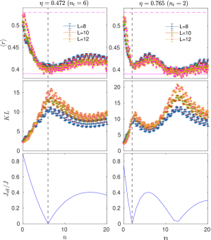
Figure 4: Level statistic $r$ (top) and Kullback-Leibler divergence (KL) (middle) for $n_{t}=6$ (left) and $n_{t}=2$ (right) as a function of energy, compared with hopping strength $J_{\mathrm{eff}}$ obtained from the HFE (bottom). Both large and small target photon number show evidence of localization when energy is chosen to get coherent destruction of tunneling, $J_{\mathrm{eff}}\approx 0$. Localization is stronger for $n_{t}=6$, which we attribute to a smaller relative fluctuation of the photon number at higher energy. Note that the model has been slightly modified compared to other figures, namely $J\to-J$ and $\sum_{j}jn_{j}\to\sum_{j}(-1)^{j}n_{j}/2$, as described in the text.

While the regime of MBL or, at least, significant slowing down of the dynamics remain only loosely clear, what is clear is that localization is favored by small $J_{\mathrm{eff}}$ at high energy. This model therefore illustrates a variant of the inverted mobility edge that we found in an earlier work MBLCentral2 , namely that such centrally coupled models tend to localize at high energies and delocalize at low energies. The coherent oscillations of $J_{\mathrm{eff}}(n)$ lead to an even more interesting structure where the thermal phase can occur in multiple windows of energy, for which $J_{\mathrm{eff}}$ is above the threshold for thermalization.

Another interesting note is that there are large regions of the data where both level statistics and KL divergence seem to stay in between the MBL and ETH values with little dependence on system size. This is likely a finite size effect that will eventually flow to one phase or the other (likely the thermal phase, which is stabilized by higher-order corrections and resonances that are beyond our small size numerics). However, this model seems to have surprisingly slow finite size drifts compared to similar models in the MBL literature.

Finally, to emphasize the relevance of being able to tune localization dynamics via energy, we consider a more physically relevant observable, namely the imbalance $\mathcal{I}$, which in the absence of a cavity has been measured in multiple AMO experiments on MBL landig2016quantum; Hruby2018avalanche; Mazzucchi:16 ; PhysRevA.94.023632 . The idea is to initialize a charge density wave (CDW) with minimal wavelength, $|0101\cdots\rangle$, and then watch for relaxation of the CDW order as the system time evolves. The imbalance is defined as

$$\mathcal{I}=L^{-1}\sum_{j}\left(-1\right)^{j}\left(2\langle n_{j}\rangle-1\right),$$

which measures the order such that $\mathcal{I}=1$ in the initial state and $\mathcal{I}=0$ in thermal equilibrium. In order to modify the energy, we prepare the cavity mode in a coherent state $|\alpha\rangle$, such that the disorder-averaged energy $\overline{E}$ is

$$\overline{E}= \overline{\langle\alpha,0101\cdots|H_{D}|\alpha,0101\cdots\rangle}$$

$$= \overline{\sum_{j\text{ odd}}V_{j}}+\omega\left|\alpha\right|^{2}=\omega\left|\alpha\right|^{2},$$

Note that we have chosen an initial state with zero polarization, $\sum_{j}j\langle n_{j}\rangle=0$, such that switching from Coulomb gauge to dipole gauge does not change the initial state . Then we measure $\langle\mathcal{I}(t)\rangle$, the results of which are plotted in Figure 5 for 300-6000 realization of disorders. We see strong indications of slowing down and localization when tuning near the point with $J_{\mathrm{eff}}=0$. While this does not prove the existence of an MBL phase, it does suggests an experimentally relevant route to tuning localization dynamics in these cavity QED systems.

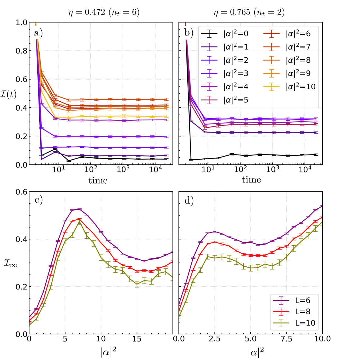
Figure 5: (a and b) Imbalance ($\mathcal{I}(t)$) as a function of time for different $|\alpha|^{2}$ and $L=10$. (c and d) Steady state value, $I(t=\infty)$. For small finite size, $\mathcal{I}(\infty)$ is nonzero, with a value that aligns well with other metrics for localization in Figure 4. For values with $J_{\mathrm{eff}}=0$ from the HFE, $\mathcal{I}(\infty)$ is large and decreases slowly with system size, consistent with many-body localized dynamics. Parameters are $\omega=8J$, $W=0.5J$ and $U=1.5J$ with constant electric field ($\eta_{j}=\eta=\mathrm{const.}$) as in the single-particle case. The initial state is a period-2 charge density wave with photons in coherent state $|\alpha\rangle$.

VI Experimental realization

As alluded to in Section II, the main experimental setup where this will be relevant is electronic systems in the strong coupling regime of cavity QED. Semiconducting nanowires are a natural situation to consider these physics, as illustrated in Figure 1. The one-dimensional nature of this model is not crucial for realizing cavity-mediated tuning of the hopping. In higher dimensional models, a similar analysis will hold, with coupling strength $\eta_{ij}$ for a given bond $<ij>$ proportional to the component of the electric field along the direction of the hopping. In two dimensions, for example, this can be used to tune lattice symmetries and connectivities, as we recently showed the case of classical drive on a moiré heterostructure GeArxiv2021 . We also note that the strong coupling regime has been achieved in electron systems, most notably cavity-mediated chemical reactions ribeiro2018polariton ; schafer2021shining , which is precisely the system for which gauge choices in cavity QED have been most actively explored gauge3 ; gauge2 ; gauge1 ; gauge .

Modifying the hopping strength will have a profound impact on the properties of these electronic systems. While molecular Hamiltonians are much more complicated than those we have written down due to strong electron-electron interactions, cavity-mediated control of the kinetic energy will still significantly modify their electron structure and many allow control of chemical reactions via tuning the strength of a cavity-pumping laser to change the intracavity photon number. In the context of nanowires, laser tuning of the photon state will directly modify transport across the wire. By gating the nanowire into a low-filling regime, the single-particle physics from Section IV may be accessible. There we expect exponential dependence of conductivity with $J_{\mathrm{eff}}$, as the transport in such single-particle localized systems is primarily through thermally activated variable range hopping Mott1969 ; Efros1975 . In both the cases of quantum chemistry and nanowires, the cavity plays an important role in enhancing the electric field strength at the electrons, allowing a strong drive regime to be accessed. A key result of our work is that the side effect of the cavity – photon-mediated long-range coupling – does not immediately destroy localization.

Cavity-induced localization may also be relevant to other cavity QED settings. It’s not likely to be immediately accessible in the context of neutral atoms, as these systems are difficult to push into the strong coupling regime. However, cavity QED with superconducting qubits, a.k.a. circuit QED, could be a useful platform to realize these physics. In that case the dipole moment of the artificial atoms, i.e., the superconducting qubits, are local to each qubit and there will not be direct hopping of the electronic excitations. Instead, the spatially dependent coupling (in the dipole gauge) could be realized by the mode profile $f(x_{j})$ of the superconducting cavity, where $x_{j}$ are the spatial locations of the superconducting qubits along the cavity. Locally interacting Bose-Hubbard models with tunable frequencies or disorder are readily realized in recent transmon experiments Chen2014 ; Roushan2014 ; Neill2016 ; Roushan2017 ; Roushan2017a . Placing an array of transmons at chosen locations along the superconducting cavity in order to realize an effective potential gradient, $f(x_{j})\propto j$, and tuning into the strong coupling regime, similar cavity-mediated localization should be realizable. In these controllable quantum systems, local measurements such as the imbalance $\mathcal{I}$ are natural, and would give a strong indication of localization dynamics.

VII conclusion

In conclusion, we studied the possibility of realizing many-body localization (MBL) in the context of strong coupling cavity QED. By working with a fermion Hubbard chain inside a high-quality cavity, we show that a variant of coherent destruction of tunneling is possible even at a moderate photon number. In the single-particle regime, this directly modulates the localization length. In the many-body regime, we show evidence that MBL survives, despite the presence of cavity-mediated long-range correlated hopping and interactions. These results should prove relevant to electronic systems coupled to optical cavities, which routinely access the strong coupling regime gauge3 ; gauge2 ; gauge1 ; gauge , and may also be relevant to superconducting circuit QED.

A major theoretical accomplishment of this work is to develop a method for integrating out the cavity photon in the presence of strong driving, which is intricately tied to the electromagnetic gauge choice made in quantizing the cavity mode. The high-frequency expansion developed here can be extended to other cases of strong and/or resonant drive, where a naive expansion in the dipole gauge would fail. A particularly interesting case where we anticipate using these results is the cavity QED realization of a quantum time crystal, in which the cavity mode plays the role of a Floquet drive. Since both the time crystal and most other non-trivial Floquet phases of matter require strong and/or resonant drive, these techniques will be valuable in understanding how these phases behave in the presence of quantized photons.

VIII Acknowledgments

The authors acknowledge useful discussions with Nathan Ng. Work was performed with support from the National Science Foundation through award number DMR-1945529 (MK and SRK) and the Welch Foundation through award number AT-2036-20200401 (MK and RG). Part of this work was performed at the Aspen Center for Physics, which is supported by National Science Foundation grant PHY-1607611, and at the Kavli Institute for Theoretical Physics, which is supported by the National Science Foundation under Grant No. NSF PHY1748958. RG is also supported by the ”Fundamental Research Funds for the Central Universities”. We used the computational resources of the Lonestar 5 cluster operated by the Texas Advanced Computing Center at the University of Texas at Austin and the Ganymede and Topo clusters operated by the University of Texas at Dallas’ Cyberinfrastructure and Research Services Department.

Appendix A Details of high-frequency expansion

We start the high-frequency expansion (HFE) using the Floquet version of our Hamiltonian, Eq. (3):

$$H_{\mathrm{rot}}(t)=\sum_{j}\left[-J\left(e^{-i\eta_{j}\left(ia^{\dagger}e^{i\omega t}-iae^{-i\omega t}\right)}c_{j}^{\dagger}c_{j+1}+h.c.\right)+Un_{j}n_{j+1}+V_{j}n_{j}\right]$$

Note that we allow position-dependent coupling $\eta_{j}$. This can capture our two main cases from the text: constant electric field, $\eta_{j}=\eta$, and staggered chemical potential, $\eta_{j}=\eta\left(-1\right)^{j}$. We recognize the photon-dependent term as the displacement operator,

$$\mathcal{D}(\alpha)=\exp\left[\alpha a^{\dagger}-\alpha^{\ast}a\right]$$

where $\alpha=\eta_{j}e^{i\omega t}$. The Hermitian conjugate ($+h.c.$) is then

$$e^{i\eta_{j}\left(-iae^{-i\omega t}+ia^{\dagger}e^{i\omega t}\right)}c_{j+1}^{\dagger}c_{j}=\mathcal{D}(-\alpha)c_{j+1}^{\dagger}c_{j}$$

where we used that $\eta_{j}$ is real. In order to do a high frequency expansion, we must expand $H_{\mathrm{rot}}$ in Fourier harmonics:

$$H_{\mathrm{rot}}(t)=\sum_{\ell}H_{\mathrm{rot}}^{(\ell)}e^{i\ell\Omega t}.$$

Let’s start by doing so for the displacement operator, from which the remainder will follow. First, note that the matrix elements of $\mathcal{D}$ in the number basis are given by Cahill1969

$$\langle m|\mathcal{D}(\alpha)|n\rangle =\begin{cases}\sqrt{\frac{n!}{m!}}\alpha^{m-n}e^{-\left|\alpha\right|^{2}/2}L_{n}^{(m-n)}\left(\left|\alpha\right|^{2}\right)&\text{for }m\geq n\\ \sqrt{\frac{m!}{n!}}\left(-\alpha\right)^{n-m}e^{-\left|\alpha\right|^{2}/2}L_{m}^{(n-m)}\left(\left|\alpha\right|^{2}\right)&\text{for }m<n\end{cases}$$

where $L_{n}^{(k)}$ are the associate Laguerre polynomials. The only time-dependence here is in the $\alpha^{m-n}$ or $\left(-\alpha\right)^{m-n}$ term. Noting that $\alpha^{m-n}=\eta_{j}^{m-n}e^{i\omega\left(m-n\right)t}$, this is clearly going to give the $\ell$th Fourier harmonic with $\ell=m-n\geq 0$. Adding together all the terms, the $\ell$th Fourier harmonic of $H_{\mathrm{rot}}$ is then

$$H_{\mathrm{rot}}^{(\ell\geq 0)} =\sum_{n=0}^{\infty}\sum_{j}\Bigg{[}-J\left(\sqrt{\frac{n!}{\left(n+\ell\right)!}}\eta_{j}^{\ell}e^{-\left|\eta_{j}\right|^{2}/2}L_{n}^{(\ell)}\left(\left|\eta_{j}\right|^{2}\right)c_{j}^{\dagger}c_{j+1}+\sqrt{\frac{n!}{\left(n+\ell\right)!}}\left(-\eta_{j}\right)^{\ell}e^{-\left|\eta_{j}\right|^{2}/2}L_{n}^{(\ell)}\left(\left|\eta_{j}\right|^{2}\right)c_{j+1}^{\dagger}c_{j}\right)$$

$$\;\;\;\;\;\;\;\;\;\;\;\;+\delta_{\ell,0}\left(Un_{j}n_{j+1}+V_{j}n_{j}\right)\Bigg{]}|n+\ell\rangle\langle n|$$

$$=\sum_{n=0}^{\infty}\sum_{j}\Bigg{[}-J\sqrt{\frac{n!}{\left(n+\ell\right)!}}\eta_{j}^{\ell}e^{-\left|\eta_{j}\right|^{2}/2}L_{n}^{(\ell)}\left(\left|\eta_{j}\right|^{2}\right)\left(c_{j}^{\dagger}c_{j+1}+\left(-1\right)^{\ell}c_{j+1}^{\dagger}c_{j}\right)+\delta_{\ell,0}\left(Un_{j}n_{j+1}+V_{j}n_{j}\right)\Bigg{]}|n+\ell\rangle\langle n|$$

$$H_{\mathrm{rot}}^{(-\ell)} =\left[H_{\mathrm{rot}}^{(\ell)}\right]^{\dagger}$$

where the last line follows from Hermitianity of $H_{\mathrm{rot}}$.

The time-average of $H_{\mathrm{rot}}$, which is the zeroth order $H_{\mathrm{eff}}$, is then easy to compute. Noting that the effective Hamiltonian has zero frequency and is, therefore, diagonal in the number basis, we can project onto the photon number state $|n\rangle$ to get

$$H_{\mathrm{eff}}^{0}(n) =\langle n|H_{\mathrm{rot}}^{(0)}|n\rangle$$

$$=\sum_{j}\Bigg{[}-\underbrace{Je^{-\left|\eta_{j}\right|^{2}/2}L_{n}\left(\left|\eta_{j}\right|^{2}\right)}_{J_{\mathrm{eff}}(n,\eta_{j})}\left(c_{j}^{\dagger}c_{j+1}+c_{j+1}^{\dagger}c_{j}\right)+Un_{j}n_{j+1}+V_{j}n_{j}\Bigg{]}$$

Note that, for both choices of $\eta_{j}$ made in paper, one gets an identical $J_{\mathrm{eff}}$ at zeroth order.

The first order correct will give rise to leading correlated hopping terms. Again, projecting onto the $n$ photon state, we have

$$H_{\mathrm{eff}}^{1}(n) =\sum_{\ell>0}\frac{\langle n|\left[H^{(\ell)},H^{(-\ell)}\right]|n\rangle}{\ell\omega}=\sum_{\ell>0}\frac{\langle n|\left[H^{(\ell)},\left(H^{(\ell)}\right)^{\dagger}\right]|n\rangle}{\ell\omega}$$

$$=\sum_{\ell>0}\frac{\langle n|H^{(\ell)}\left(H^{(\ell)}\right)^{\dagger}|n\rangle-\langle n|\left(H^{(\ell)}\right)^{\dagger}H^{(\ell)}|n\rangle}{\ell\omega}$$

$$=\sum_{\ell=1}^{n}\frac{\langle n|H^{(\ell)}|n-\ell\rangle\langle n-\ell|\left(H^{(\ell)}\right)^{\dagger}|n\rangle}{\ell\omega}-\sum_{\ell=1}^{\infty}\frac{\langle n|\left(H^{(\ell)}\right)^{\dagger}|n+\ell\rangle\langle n+\ell|H^{(\ell)}|n\rangle}{\ell\omega}$$

$$=\sum_{\ell=1}^{n}\frac{\langle n|H^{(\ell)}|n-\ell\rangle\left(\langle n|H^{(\ell)}|n-\ell\rangle\right)^{\dagger}}{\ell\omega}-\sum_{\ell=1}^{\infty}\frac{\left(\langle n+\ell|H^{(\ell)}|n\rangle\right)^{\dagger}\langle n+\ell|H^{(\ell)}|n\rangle}{\ell\omega}$$

$$=\frac{J^{2}}{\omega}\sum_{\ell=1}^{n}\frac{\left(n-\ell\right)!}{\ell n!}\sum_{j,j^{\prime}}L_{n-\ell}^{(\ell)}\left(\left|\eta_{j}\right|^{2}\right)L_{n-\ell}^{(\ell)}\left(\left|\eta_{j^{\prime}}\right|^{2}\right)\eta_{j}^{\ell}\eta_{j^{\prime}}^{\ell}e^{-\left(\left|\eta_{j}\right|^{2}+\left|\eta_{j^{\prime}}\right|^{2}\right)/2}\times$$

$$\;\;\;\;\;\;\;\;\;\;\;\;\;\;\;\;\times\left(-1\right)^{\ell}\left(c_{j}^{\dagger}c_{j+1}+\left(-1\right)^{\ell}c_{j+1}^{\dagger}c_{j}\right)\left(c_{j^{\prime}}^{\dagger}c_{j^{\prime}+1}+\left(-1\right)^{\ell}c_{j^{\prime}+1}^{\dagger}c_{j^{\prime}}\right)$$

$$\;\;\;\;\;-\frac{J^{2}}{\omega}\sum_{\ell=1}^{\infty}\frac{n!}{\ell\left(n+\ell\right)!}\sum_{j,j^{\prime}}L_{n}^{(\ell)}\left(\left|\eta_{j}\right|^{2}\right)L_{n}^{(\ell)}\left(\left|\eta_{j^{\prime}}\right|^{2}\right)\eta_{j}^{\ell}\eta_{j^{\prime}}^{\ell}e^{-\left(\left|\eta_{j}\right|^{2}+\left|\eta_{j^{\prime}}\right|^{2}\right)/2}\times$$

$$\;\;\;\;\;\;\;\;\;\;\;\;\;\;\;\;\times\left(-1\right)^{\ell}\left(c_{j}^{\dagger}c_{j+1}+\left(-1\right)^{\ell}c_{j+1}^{\dagger}c_{j}\right)\left(c_{j^{\prime}}^{\dagger}c_{j^{\prime}+1}+\left(-1\right)^{\ell}c_{j^{\prime}+1}^{\dagger}c_{j^{\prime}}\right)$$

In order to simplify this expression, let’s consider the simplest case that $\eta_{j}=\eta$ is constant. Then

$$\begin{split}H_{\mathrm{eff}}^{1}(n)&=\frac{J^{2}}{\omega}\sum_{\ell=1}^{n}\frac{\left(-1\right)^{\ell}}{\ell}\left[\frac{\left(n-\ell\right)!}{n!}\left(L_{n-\ell}^{(\ell)}\left(\eta^{2}\right)\right)^{2}-\frac{n!}{\left(n+\ell\right)!}\left(L_{n}^{(\ell)}\left(\eta^{2}\right)\right)^{2}\right]\eta^{2\ell}e^{-\eta^{2}}\times\\ &\;\;\;\;\;\;\;\;\;\;\;\;\;\;\;\;\times\sum_{j,j^{\prime}}\left(c_{j}^{\dagger}c_{j+1}+\left(-1\right)^{\ell}c_{j+1}^{\dagger}c_{j}\right)\left(c_{j^{\prime}}^{\dagger}c_{j^{\prime}+1}+\left(-1\right)^{\ell}c_{j^{\prime}+1}^{\dagger}c_{j^{\prime}}\right)\\ &\;\;\;\;\;-\frac{J^{2}}{\omega}\sum_{\ell=n}^{\infty}\frac{\left(-1\right)^{\ell}n!}{\ell\left(n+\ell\right)!}\left(L_{n}^{(\ell)}\left(\eta^{2}\right)\right)^{2}\eta^{2\ell}e^{-\eta^{2}}\sum_{j,j^{\prime}}\left(c_{j}^{\dagger}c_{j+1}+\left(-1\right)^{\ell}c_{j+1}^{\dagger}c_{j}\right)\left(c_{j^{\prime}}^{\dagger}c_{j^{\prime}+1}+\left(-1\right)^{\ell}c_{j^{\prime}+1}^{\dagger}c_{j^{\prime}}\right)\\ &=-\frac{J^{2}e^{-\eta^{2}}}{\omega}\left(\sum_{\ell=1,3,\cdots}\frac{f(n,\ell,\eta)}{\ell}\eta^{2\ell}\right)\left[\sum_{j}\left(c_{j}^{\dagger}c_{j+1}-c_{j+1}^{\dagger}c_{j}\right)\right]^{2}\\ &\;\;\;+\frac{J^{2}e^{-\eta^{2}}}{\omega}\left(\sum_{\ell=2,4,\cdots}\frac{f(n,\ell,\eta)}{\ell}\eta^{2\ell}\right)\left[\sum_{j}\left(c_{j}^{\dagger}c_{j+1}+c_{j+1}^{\dagger}c_{j}\right)\right]^{2}\end{split}$$ (5)

where

$$f(n,\ell,\eta)=\begin{cases}\frac{\left(n-\ell\right)!}{n!}\left(L_{n-\ell}^{(\ell)}\left(\eta^{2}\right)\right)^{2}-\frac{n!}{\left(n+\ell\right)!}\left(L_{n}^{(\ell)}\left(\eta^{2}\right)\right)^{2}&\text{if }\ell\leq n\\ -\frac{n!}{\left(n+\ell\right)!}\left(L_{n}^{(\ell)}\left(\eta^{2}\right)\right)^{2}&\text{if }\ell>n\end{cases}$$

The case $\eta_{j}=\left(-1\right)^{j}$ is quite similar, except with an additional distinction between hopping sign for even and odd sites. From Eq. 5, we can define the effective long-range coupling as

$$g_{\mathrm{eff}}^{\mathrm{I}} =e^{-\eta^{2}}\sum_{\ell=1,3,\cdots}\frac{f(n,\ell,\eta)}{\ell}\eta^{2\ell}$$ (6)

$$g_{\mathrm{eff}}^{\mathrm{R}} =e^{-\eta^{2}}\sum_{\ell=2,4,\cdots}\frac{f(n,\ell,\eta)}{\ell}\eta^{2\ell}$$ (7)

where the labels R and I denote that the corresponding correlated hopping terms have real and imaginary phase, respectively. The behavior of these $g_{\mathrm{eff}}$ couplings as a function of $\eta$ is shown in Figure 6. For any $n$, the coupling constants clearly vanish at large $\tilde{\eta}$, meaning that strong coupling eliminates long-range correlated hopping as well as nearest neighbor hopping. Combined with our arguments for the appropriate scaling of $g$ with $L$ (see main text), this provides further analytical support for the possibility of MBL in the strong coupling regime, even for the extreme quantum limit of photons in their ground state ($n=0$). Note, however, that at medium coupling strengths $\tilde{\eta}\sim 1$, $g_{\mathrm{eff}}$ for the real and imaginary terms do not vanish at the same values of $\tilde{\eta}$, implying that the fine-tuned physics of coherent destruction of tunneling do not simply persist in these higher order terms.

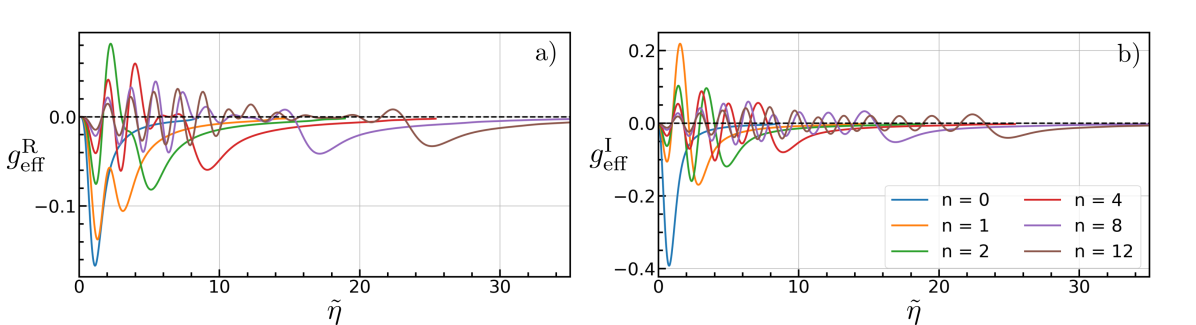
Figure 6: Effective long-range hopping coefficient $g_{\mathrm{eff}}$ as a function of rescaled drive strength $\tilde{\eta}$ for various photon numbers. At large drive strength, $\tilde{\eta}\gg 1$, the long-range correlated hopping is switched off, favoring localization.

We are often interested in the large-$n$ expansion of this effective long-range coupling, since that will tell us about the semi-classical limit of the cavity photons. Noting that $\eta=\tilde{\eta}/\sqrt{n+1/2}$, a large $n$ expansion corresponds to $\eta\ll 1$. Thus, at leading order, we simply have $e^{-\eta^{2}}\approx 1$. Then the relevant term is $f(n,\ell,\eta)\eta^{2\ell}$. We will see this is dominated by small $\ell$, so for now restrict ourselves to $\ell\ll n$. Writing out the associated Legendre polynomial,

$$L_{n}^{(\ell)}\left(\eta^{2}\right)=\sum_{m=0}^{n}\frac{\left(-\eta^{2}\right)^{m}\left(n+\ell\right)!}{\left(n-m\right)!m!\left(\ell+m\right)!}$$ (8)

Taking this at second order in $\eta\ll 1$ (i.e., up to $m=2$), we have

$$L_{n}^{(\ell)}\left(\eta^{2}\right) =\frac{\left(n+\ell\right)!}{n!\ell!}-\eta^{2}\frac{\left(n+\ell\right)!}{\left(n-1\right)!\left(\ell+1\right)!}+\frac{\eta^{4}}{2}\frac{\left(n+\ell\right)!}{\left(n-2\right)!\left(\ell+2\right)!}+O\left(\eta^{6}\right)$$ (9)

$$=\frac{\left(n+\ell\right)!}{n!\ell!}\left[1-\frac{\eta^{2}n}{\ell+1}+\frac{\eta^{4}n\left(n-1\right)}{\left(\ell+1\right)\left(\ell+2\right)}+O\left(\eta^{6}\right)\right]$$ (10)

$$\left[L_{n}^{(\ell)}\left(\eta^{2}\right)\right]^{2} =\left(\frac{\left(n+\ell\right)!}{n!\ell!}\right)^{2}\left[1-\eta^{2}\frac{2n}{\ell+1}+\eta^{4}\frac{2n\left(n-1\right)\left(\ell+1\right)+n^{2}\left(\ell+2\right)}{\left(\ell+1\right)^{2}\left(\ell+2\right)}+O\left(\eta^{6}\right)\right]$$ (11)

Notice that each term in the square brackets is independent of $n$ in the limit $n\gg\ell$, since $\eta^{2}\approx\tilde{\eta}^{2}/n$. Furthermore, higher order terms $\sim\eta^{2m}$ quickly vanish for $m\gg 1$ due to the factorial appearing in the denominator.

When we combine terms to get $f$, we see that (for $\ell\ll n$)

$$f(n,\ell,\eta) =\frac{n!}{\left(n-\ell\right)!\left(\ell!\right)^{2}}\left[1-\eta^{2}\frac{2\left(n-\ell\right)}{\ell+1}+\eta^{4}\frac{2\left(n-\ell\right)\left(n-\ell-1\right)\left(\ell+1\right)+\left(n-\ell\right)^{2}\left(\ell+2\right)}{\left(\ell+1\right)^{2}\left(\ell+2\right)}+O\left(\eta^{6}\right)\right]$$ (12)

$$\;\;\;\;-\frac{\left(n+\ell\right)!}{n!\left(\ell!\right)^{2}}\left[1-\eta^{2}\frac{2n}{\ell+1}+\eta^{4}\frac{2n\left(n-1\right)\left(\ell+1\right)+n^{2}\left(\ell+2\right)}{\left(\ell+1\right)^{2}\left(\ell+2\right)}+O\left(\eta^{6}\right)\right]$$ (13)

Note that, at leading order in $n^{-1}$, we just get $f=0$. Therefore, we need to expand it to first order:

$$\frac{n!}{\left(n-\ell\right)!} =n(n-1)\cdots(n-\ell+1)=n^{\ell}+n^{\ell-1}\left(-1-2-\cdots-\left(\ell-1\right)\right)+O\left(n^{\ell-2}\right)$$ (14)

$$=n^{\ell}-n^{\ell-1}\frac{\ell\left(\ell-1\right)}{2}+O\left(n^{\ell-2}\right)$$ (15)

$$\eta^{2m} =\frac{\tilde{\eta}^{2m}}{\left(n+1/2\right)^{m}}=\frac{\tilde{\eta}^{2m}}{n^{m}}\left(1+\frac{1}{2n}\right)^{-m}=\frac{\tilde{\eta}^{2m}}{n^{m}}\left(1-\frac{m}{2n}+O\left(n^{-2}\right)\right)$$ (16)

$$\left(\ell!\right)^{2}f(n,\ell,\eta) \approx\left(n^{\ell}-n^{\ell-1}\frac{\ell\left(\ell-1\right)}{2}\right)\Bigg{[}1-\frac{2\tilde{\eta}^{2}\left(1-\frac{1}{2n}\right)\left(1-\frac{\ell}{n}\right)}{\left(\ell+1\right)}\;+$$ (17)

$$\;\;\;\;\;\;\;\;\;\;\;\;\;\;\;\;\;\;\;\;\;\;\;\;\;\;\;\;\frac{\tilde{\eta}^{4}\left(1-\frac{1}{n}\right)\left[2\left(\ell+1\right)\left(1-\frac{2\ell+1}{n}\right)+\left(1-\frac{2\ell}{n}\right)\left(\ell+2\right)\right]}{\left(\ell+1\right)^{2}\left(\ell+2\right)}+O\left(\eta^{6}\right)\Bigg{]}\;-$$ (18)

$$\;\;\;\;\left(n^{\ell}+n^{\ell-1}\frac{\ell\left(\ell+1\right)}{2}\right)\left[1-\frac{2\tilde{\eta}^{2}\left(1-\frac{1}{2n}\right)}{\left(\ell+1\right)}+\frac{\tilde{\eta}^{4}\left(1-\frac{1}{n}\right)\left[2\left(1-\frac{1}{n}\right)\left(\ell+1\right)+\left(\ell+2\right)\right]}{\left(\ell+1\right)^{2}\left(\ell+2\right)}+O\left(\eta^{6}\right)\right]$$ (19)

$$=n^{\ell-1}F\left(\ell,\tilde{\eta}\right)+O\left(n^{\ell-2}\right)$$ (20)

where we see explicitly that the term proportional to $n^{\ell}$ cancels out. Finally, we find the leading correction to the long-range interaction is

$$g_{\mathrm{eff}}^{s} \approx s\frac{J^{2}}{\omega}\left(\sum_{\ell_{s}}\left[\frac{n^{\ell-1}F\left(\ell,\tilde{\eta}\right)}{\ell\left(\ell!\right)^{2}}+O\left(n^{\ell-2}\right)\right]\eta^{2\ell}\right)$$ (21)

$$=s\frac{J^{2}}{n\omega}\left(\sum_{\ell_{s}}\frac{F\left(\ell,\tilde{\eta}\right)\tilde{\eta}^{2\ell}}{\ell\left(\ell!\right)^{2}}\right)+O\left(n^{-2}\right)$$ (22)

where $s=\pm 1$ tells us whether to sum over even ($s=1$) or odd ($s=-1$) terms. As expected, the leading correction at fixed $\tilde{\eta}$ goes as $1/\left(n\omega\right)$ for large $n$. Notice that this vanishes very quickly for $\ell\gg 1$, so there is no need to consider any limit besides $\ell\ll n$.

Appendix B Role of gauge freedom in many-body localization

Most papers on cavity QED implicitly work in the dipole gauge yet neglect the $P^{2}$ term. A generic such Hamiltonian can be written

$$H_{\tilde{D}}^{gen}=\sum_{j}\left[\frac{p_{j}^{2}}{2m}+V({\bf r_{j}})-\omega q{\bf r}_{j}\cdot{\bf f}({\bf r}_{j})\left(a+a^{\dagger}\right)\right]+\omega a^{\dagger}a$$

where we will use the convention that a tilde over the gauge label indicates this missing term. Truncating this Hamiltonian to get a Fermi-Hubbard model similar to that in the main text, one finds

$$H_{\tilde{D}}=\sum_{j}\left[-J\left(c_{j}^{\dagger}c_{j+1}+h.c.\right)+Un_{j}n_{j+1}+V_{j}n_{j}-\omega\eta jn_{j}\left(a+a^{\dagger}\right)\right]+\omega a^{\dagger}a$$ (23)

which seems natural. However, we will soon see that this incorrect quantization leads to significant differences, including qualitative changes in the ability to localize the system.

We can move to the Coulomb gauge by the same gauge transformation as before, $U_{PZW}=\exp\left[-i\sum_{j}qdjn_{j}f_{0}\left(ia^{\dagger}-ia\right)\right]$. But now we find

$$H_{\tilde{C}}=\sum_{j}\left[-J\left(e^{-i\eta\left(ia^{\dagger}-ia\right)}c_{j}^{\dagger}c_{j+1}+h.c.\right)+Un_{j}n_{j+1}+V_{j}n_{j}\right]+\omega a^{\dagger}a-\omega\left(\sum_{j}\eta jn_{j}\right)^{2}.$$ (24)

In other words, the infinite range $P^{2}$ interaction appears in the Coulomb gauge, albeit with opposite sign as in the correct quantization. This is problematic for a number of reasons. First, it kills translation invariance in this gauge, where it is expected on physical grounds. Second, it remains untouched in the high-frequency expansion, which must be done in the Coulomb gauge for strong drive, as we saw in the main text. Therefore, even at zeroth order, one finds long-range interactions which compete with hopping and local interactions:

$$H_{\mathrm{eff}}^{0}=\sum_{j}\left[-J_{\mathrm{eff}}\left(c_{j}^{\dagger}c_{j+1}+h.c.\right)+Un_{j}n_{j+1}+V_{j}n_{j}\right]-\omega\left(\sum_{j}\eta jn_{j}\right)^{2}$$

Indeed, the existence of this last term calls the high-frequency expansion into question, as it is large (proportional to $\omega$) yet has not been made diagonal by the canonical transformation.

The effects of this term also show up numerically. As seen in Figure 7, the system shows little sign of localization in the presence of this additional term, even in the case where one has nearly perfect coherent destruction of tunneling ($E/\omega\approx n_{t}$). This seems to be due to the additional long-range interactions, which make localization fragile.

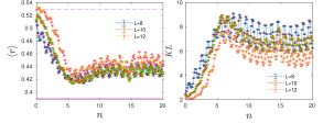
Figure 7: Level statistics (left) and Kullback-Leibler divergence (KL) (right) for $n_{t}=6$ when using the incorrect quantization, shown in Eqs. 23 and 24. Parameters are similar to those in Figure 4, except that $n_{t}=5.523$ ($\eta=0.49$).

References

- (1) I. Bloch, J. Dalibard, and W. Zwerger, Many-body physics with ultracold gases, Rev. Mod. Phys. 80, 885 (2008).
- (2) J. Dalibard, F. Gerbier, G. Juzeliunas, and P. Ohberg, Colloquium: Artificial gauge potentials for neutral atoms, Rev. Mod. Phys. 83, 1523 (2011).
- (3) M. S. Rudner, N. H. Lindner, E. Berg, and M. Levin, Anomalous edge states and the bulk-edge correspondence for periodically driven two-dimensional systems, Phys. Rev. X 3, 031005 (2013).
- (4) R. Roy and F. Harper, Abelian floquet symmetry-protected topological phases in one dimension, Phys. Rev. B 94, 125105 (2016).
- (5) C. W. von Keyserlingk and S. L. Sondhi, Phase structure of one-dimensional interacting floquet systems. i. abelian symmetry-protected topological phases, Phys. Rev. B 93, 245145 (2016).
- (6) D. V. Else and C. Nayak, Classification of topological phases in periodically driven interacting systems, Phys. Rev. B 93, 201103 (2016).
- (7) A. C. Potter, T. Morimoto, and A. Vishwanath, Classification of interacting topological floquet phases in one dimension, Phys. Rev. X 6, 041001 (2016).
- (8) F. Nathan and M. S. Rudner, Topological singularities and the general classification of floquet-bloch systems, New J. Phys. 17, 125014 (2015).
- (9) R. Roy and F. Harper, Periodic table for floquet topological insulators, Phys. Rev. B 96, 155118 (2017).
- (10) P. Titum, E. Berg, M. S. Rudner, G. Refael, and N. H. Lindner, Anomalous floquet-anderson insulator as a nonadiabatic quantized charge pump, Phys. Rev. X 6, 021013 (2016).
- (11) H. C. Po, L. Fidkowski, T. Morimoto, A. C. Potter, and A. Vishwanath, Chiral floquet phases of many-body localized bosons, Phys. Rev. X 6, 041070 (2016).
- (12) A. C. Potter and T. Morimoto, Dynamically enriched topological orders in driven two-dimensional systems, Phys. Rev. B 95, 155126 (2017).
- (13) F. Harper and R. Roy, Floquet topological order in interacting systems of bosons and fermions, Phys. Rev. Lett. 118, 115301 (2017).
- (14) R. Roy and F. Harper, Floquet topological phases with symmetry in all dimensions, Phys. Rev. B 95, 195128 (2017).
- (15) H. C. Po, L. Fidkowski, A. Vishwanath, and A. C. Potter, Radical chiral floquet phases in a periodically driven kitaev model and beyond, Phys. Rev. B 96, 245116 (2017).
- (16) A. C. Potter, A. Vishwanath, and L. Fidkowski, Infinite family of three-dimensional floquet topological paramagnets, Phys. Rev. B 97, 245106 (2018).
- (17) D. Reiss, F. Harper, and R. Roy, Interacting floquet topological phases in three dimensions, Phys. Rev. B 98, 045127 (2018).
- (18) M. H. Kolodrubetz, F. Nathan, S. Gazit, T. Morimoto, and J. E. Moore, Topological floquet-thouless energy pump, Phys. Rev. Lett. 120, 150601 (2018).
- (19) F. Nathan, D. Abanin, E. Berg, N. H. Lindner, and M. S. Rudner, Anomalous floquet insulators, Phys. Rev. B 99, 195133 (2019).
- (20) C. I. Timms, L. M. Sieberer, and M. H. Kolodrubetz, Quantized floquet topology with temporal noise, Phys. Rev. Lett. 127, 270601 (2021).
- (21) D. M. Long, P. J. D. Crowley, and A. Chandran, Nonadiabatic topological energy pumps with quasiperiodic driving, Phys. Rev. Lett. 126, 106805 (2021).
- (22) F. Nathan, R. Ge, S. Gazit, M. Rudner, and M. Kolodrubetz, Quasiperiodic floquet-thouless energy pump, Phys. Rev. Lett. 127, 166804 (2021).
- (23) V. Khemani, A. Lazarides, R. Moessner, and S. L. Sondhi, Phase structure of driven quantum systems, Phys. Rev. Lett. 116, 250401 (2016).
- (24) C. W. von Keyserlingk and S. L. Sondhi, Phase structure of one-dimensional interacting floquet systems. ii. symmetry-broken phases, Phys. Rev. B 93, 245146 (2016).
- (25) D. V. Else, B. Bauer, and C. Nayak, Floquet time crystals, Phys. Rev. Lett. 117, 090402 (2016).
- (26) S. Choi, J. Choi, R. Landig, G. Kucsko, H. Zhou, J. Isoya, F. Jelezko, S. Onoda, H. Sumiya, V. Khemani, et al., Observation of discrete time-crystalline order in a disordered dipolar many-body system, Nature 543, 221 (2017).
- (27) J. Zhang, P. W. Hess, A. Kyprianidis, P. Becker, A. Lee, J. Smith, G. Pagano, I.-D. Potirniche, A. C. Potter, A. Vishwanath, et al., Observation of a discrete time crystal, Nature 543, 217 (2017).
- (28) D. V. Else, C. Monroe, C. Nayak, and N. Y. Yao, Discrete time crystals, Annu. Rev. Condens. Matter Phys. 11, 467 (2020).
- (29) V. Khemani, R. Moessner, and S. L. Sondhi, A brief history of time crystals, arXiv:1910.10745.
- (30) X. Mi, M. Ippoliti, C. Quintana, A. Greene, Z. Chen, J. Gross, F. Arute, K. Arya, J. Atalaya, R. Babbush, et al., Time-crystalline eigenstate order on a quantum processor, Nature 601, 531 (2022).
- (31) A. Rubio-Abadal, M. Ippoliti, S. Hollerith, D. Wei, J. Rui, S. L. Sondhi, V. Khemani, C. Gross, and I. Bloch, Floquet prethermalization in a bose-hubbard system, Phys. Rev. X 10, 021044 (2020).
- (32) P. Peng, C. Yin, X. Huang, C. Ramanathan, and P. Cappellaro, Floquet prethermalization in dipolar spin chains, Nat. Phys. 17, 444 (2021).
- (33) W. Beatrez, O. Janes, A. Akkiraju, A. Pillai, A. Oddo, P. Reshetikhin, E. Druga, M. McAllister, M. Elo, B. Gilbert, D. Suter, and A. Ajoy, Floquet prethermalization with lifetime exceeding 90 s in a bulk hyperpolarized solid, Phys. Rev. Lett. 127, 170603 (2021).
- (34) M. Bukov, M. Heyl, D. A. Huse, and A. Polkovnikov, Heating and many-body resonances in a periodically driven two-band system, Phys. Rev. B 93, 155132 (2016).
- (35) S. A. Weidinger and M. Knap, Floquet prethermalization and regimes of heating in a periodically driven, interacting quantum system (2017).
- (36) C. J. Turner, A. A. Michailidis, D. A. Abanin, M. Serbyn, and Z. Papic, Weak ergodicity breaking from quantum many-body scars, Nat. Phys. 14, 745 (2018).
- (37) R. M. Nandkishore and M. Hermele, Fractons, Annu. Rev. Condens. Matter Phys. 10, 295 (2019).
- (38) P. Ponte, Z. Papic, F. Huveneers, and D. A. Abanin, Many-body localization in periodically driven systems, Phys. Rev. Lett. 114, 140401 (2015).
- (39) A. Lazarides, A. Das, and R. Moessner, Fate of many-body localization under periodic driving, Phys. Rev. Lett. 115, 030402 (2015).
- (40) D. A. Abanin, W. De Roeck, and F. Huveneers, Theory of many-body localization in periodically driven systems, Ann. Phys. 372, 1 (2016).
- (41) C. Chen, F. Burnell, and A. Chandran, How does a locally constrained quantum system localize?, Phys. Rev. Lett. 121, 085701 (2018).
- (42) N. Ng and M. Kolodrubetz, Many-body localization in the presence of a central qudit, Phys. Rev. Lett. 122, 240402 (2019).
- (43) S. R. Koshkaki and M. H. Kolodrubetz, Inverted many-body mobility edge in a central qudit problem, Phys. Rev. B 105, L060303 (2022).
- (44) N. Ng, S. Wenderoth, R. R. Seelam, E. Rabani, H.-D. Meyer, M. Thoss, and M. Kolodrubetz, Localization dynamics in a centrally coupled system, Phys. Rev. B 103, 134201 (2021).
- (45) P. Kubala, P. Sierant, G. Morigi, and J. Zakrzewski, Ergodicity breaking with long-range cavity-induced quasiperiodic interactions, Phys. Rev. B 103, 174208 (2021).
- (46) F. Grossmann, T. Dittrich, P. Jung, and P. HAcnggi, Coherent destruction of tunneling, Phys. Rev. Lett. 67, 516 (1991).
- (47) H. Lignier, C. Sias, D. Ciampini, Y. Singh, A. Zenesini, O. Morsch, and E. Arimondo, Dynamical control of matter-wave tunneling in periodic potentials, Phys. Rev. Lett. 99, 220403 (2007).
- (48) D. De Bernardis, P. Pilar, T. Jaako, S. De Liberato, and P. Rabl, Breakdown of gauge invariance in ultrastrong-coupling cavity qed, Phys. Rev. A 98, 053819 (2018).
- (49) M. A. D. Taylor, A. Mandal, W. Zhou, and P. Huo, Resolution of gauge ambiguities in molecular cavity quantum electro- dynamics, Phys. Rev. Lett. 125, 123602 (2020).
- (50) O. Di Stefano, A. Settineri, V. Macri, L. Garziano, R. Stassi, S. Savasta, and F. Nori, Resolution of gauge ambiguities in ultrastrong-coupling cavity quantum electrodynamics, Nat. Phys. 15, 803 (2019).
- (51) A. Stokes and A. Nazir, Gauge ambiguities imply jaynes-cummings physics remains valid in ultrastrong coupling qed, Nat. commun. 10, 1 (2019).
- (52) M. Bukov, M. Kolodrubetz, and A. Polkovnikov, Schrieffer-wolff transformation for periodically driven systems: Strongly correlated systems with artificial gauge fields, Phys. Rev. Lett. 116, 125301 (2016).
- (53) M. Bukov, L. DÁlessio, and A. Polkovnikov, Universal high-frequency behavior of periodically driven systems: from dynamical stabilization to floquet engineering, Adv. Phys. 64, 139 (2015).
- (54) N. Goldman and J. Dalibard, Periodically driven quantum systems: Effective hamiltonians and engineered gauge fields, Phys. Rev. X 4, 031027 (2014).
- (55) E. Bairey, G. Refael, and N. H. Lindner, Driving induced many-body localization, Phys. Rev. B 96, 020201 (2017).
- (56) D. S. Bhakuni, R. Nehra, and A. Sharma, Drive-induced many-body localization and coherent destruction of Stark many-body localization, Phys. Rev. B 102, 024201 (2020).
- (57) R. Nandkishore and D. A. Huse, Many-body localization and thermalization in quantum statistical mechanics, Annu. Rev. Condens. Matter Phys. 6, 15 (2015).
- (58) J. Å untajs, J. Bonca, T. Prosen, and L. Vidmar, Quantum chaos challenges many-body localization, Phys. Rev. E 102, 062144 (2020).
- (59) D. Sels and A. Polkovnikov, Dynamical obstruction to localization in a disordered spin chain, Phys. Rev. E 104, 054105 (2021).
- (60) T. LeBlond, D. Sels, A. Polkovnikov, and M. Rigol, Universality in the onset of quantum chaos in many-body systems, Phys. Rev. B 104, L201117 (2021).
- (61) J. M. Deutsch, Quantum statistical mechanics in a closed system, Phys. Rev. A 43, 2046 (1991).
- (62) M. Srednicki, Chaos and quantum thermalization, Phys. Rev. E 50, 888 (1994).
- (63) M. Rigol, V. Dunjko, and M. Olshanii, Thermalization and its mechanism for generic isolated quantum systems, Nature 452, 854 (2008).
- (64) V. Oganesyan and D. A. Huse, Localization of interacting fermions at high temperature, Phys. Rev. B 75, 155111 (2007).
- (65) A. Pal and D. A. Huse, Many-body localization phase transition, Phys. Rev. B 82, 174411 (2010).
- (66) D. J. Luitz, N. Laflorencie, and F. Alet, Many-body localization edge in the random-field heisenberg chain, Phys. Rev. B 91, 081103 (2015).
- (67) F. Alet and N. Laflorencie, Many-body localization: An introduction and selected topics, Comptes Rendus Physique 19, 498 (2018), quantum simulation / Simulation quantique.
- (68) R. Landig, L. Hruby, N. Dogra, M. Landini, R. Mottl, T. Donner, and T. Esslinger, Quantum phases from competing short-and long-range interactions in an optical lattice, Nature 532, 476 (2016).
- (69) L. Hruby, N. Dogra, M. Landini, T. Donner, and T. Esslinger, Metastability and avalanche dynamics in strongly correlated gases with long-range interactions, Proceedings of the National Academy of Sciences 115, 3279 (2018),
- (70) G. Mazzucchi, S. F. Caballero-Benitez, D. A. Ivanov, and I. B. Mekhov, Quantum optical feedback control for creating strong correlations in many-body systems, Optica 3, 1213 (2016).
- (71) N. Dogra, F. Brennecke, S. D. Huber, and T. Donner, Phase transitions in a bose-hubbard model with cavity-mediated global-range interactions, Phys. Rev. A 94, 023632 (2016).
- (72) In practice we do this by choosing to define j = 0 such that polarization vanishes, even if that means the origin lies between sites. This choice has no effect on the physics, but makes the calculation easier.
- (73) R.-C. Ge and M. Kolodrubetz, Floquet engineering of lattice structure and dimensionality in twisted moiré heterobilayers, arXiv:2103.09874.
- (74) R. F. Ribeiro, L. A. Martinez-Martinez, M. Du, J. Campos-Gonzalez-Angulo, and J. Yuen-Zhou, Polariton chemistry: controlling molecular dynamics with optical cavities, Chemical science 9, 6325 (2018).
- (75) C. Schafer, J. Flick, E. Ronca, P. Narang, and A. Rubio, Shining light on the microscopic resonant mechanism responsible for cavity-mediated chemical reactivity, arXiv preprint arXiv:2104.12429 (2021).
- (76) N. F. Mott, Conduction in non-crystalline materials, Philos Mag. 19, 835 (1969).
- (77) A. L. Efros and B. I. Shklovskii, Coulomb gap and low temperature conductivity of disordered systems, J. Phys. C: Solid State Phys. 8, L49 (1975).
- (78) Y. Chen, C. Neill, P. Roushan, N. Leung, M. Fang, R. Barends, J. Kelly, B. Campbell, Z. Chen, B. Chiaro, et al., Qubit architecture with high coherence and fast tunable coupling, Phys. Rev. Lett. 113, 220502 (2014).
- (79) P. Roushan, C. Neill, Y. Chen, M. Kolodrubetz, C. Quintana, N. Leung, M. Fang, R. Barends, B. Campbell, Z. Chen, et al., Observation of topological transitions in interacting quantum circuits, Nature 515, 241 (2014).
- (80) C. Neill, P. Roushan, M. Fang, Y. Chen, M. Kolodrubetz, Z. Chen, A. Megrant, R. Barends, B. Campbell, B. Chiaro, et al., Ergodic dynamics and thermalization in an isolated quantum system, Nat. Phys. 12, 1037 (2016).
- (81) P. Roushan, C. Neill, A. Megrant, Y. Chen, R. Babbush, R. Barends, B. Campbell, Z. Chen, B. Chiaro, A. Dunsworth, et al., Chiral ground-state currents of interacting photons in a synthetic magnetic field, Nat. Phys. 13, 146 (2017).
- (82) P. Roushan, C. Neill, J. Tangpanitanon, M. Bastidas V., A. Megrant, R. Barends, Y. Chen, Z. Chen, B. Chiaro, A. Dunsworth, et al., Spectroscopic signatures of localization with interacting photons in superconducting qubits, Science 358, 1175 (2017).
- (83) K. E. Cahill and R. J. Glauber, Ordered expansions in boson amplitude operators, Phys. Rev, 177, 1857 (1969).