Emergent orbital magnetization in Kitaev quantum magnets

Abstract

Unambiguous identification of the Kitaev quantum spin liquid (QSL) in materials remains a huge challenge despite many encouraging signs from various measurements. To facilitate the experimental detection of the Kiteav QSL, here we propose to use remnant charge response in Mott insulators hosting QSL to identify the key signatures of QSL. We predict an emergent orbital magnetization in a Kitaev system in an external magnetic field. The direction of the orbital magnetization can be flipped by rotating the external magnetic field in the honeycomb plane. The orbital magnetization is demonstrated explicitly through a detailed microscopic analysis of the multiorbital Hubbard-Kanamori Hamiltonian and also supported by a phenomenological picture. We first derive the localized electrical loop current operator in terms of the spin degrees of freedom. Thereafter, utilizing the Majorana representation, we estimate the loop currents in the ground state of the chiral Kitaev QSL state, and obtain the consequent current textures, which are responsible for the emergent orbital magnetization. Finally, we discuss the possible experimental techniques to visualize the orbital magnetization which can be considered as the signatures of the underlying excitations.

I Introduction

Understanding quantum spin liquid (QSL) states and identifying them  Balents (2010); Savary and Balents (2016); Zhou et al. (2017); Takagi et al. (2019) in materials, has become a centerpiece of research in modern condensed matter physics. The QSL is a topologically ordered state with long-range entanglement that appears in spin systems with frustrated magnetic interactions. Although the beginning of the exploration of various QSL states dates back to the seminal work by Anderson on resonating valence bond states in antiferromagnetic Mott insulators Anderson (1973), the research in QSLs rapidly intensified with the discovery of high-T_c cuprates Bednorz and Müller (1986) due to its possible connection to the origin of superconductivity Baskaran et al. (1987). Over the last four decades, various theoretical proposals Kalmeyer and Laughlin (1987); Affleck and Marston (1988); Senthil and Fisher (2000, 2001) have been made to understand this exotic phase of matter. All these works hinge on a universal consensus about the fractional nature of quasiparticles in a typical QSL state. However, an unambiguous material-based realization of a QSL phase is hitherto absent.

Among the zoo of various predicted QSL states, the Kitaev spin liquid Kitaev (2006) plays a special role. It is an exactly solvable $S=1/2$ spin model on a two-dimensional honeycomb lattice, in which the spins fractionalize into (i) Majorana fermions and (ii) $\mathbb{Z}_{2}$ vortices, also known as visons. Recently, substantial interest has emerged in the study of the Kitaev model owing to its potential realization in a few spin-orbit coupled Mott insulators such as complex iridates A₂IrO₃ Singh et al. (2012) (A = Na, Li) and $\alpha$-RuCl₃ Banerjee et al. (2016). For real materials, however, non-Kitaev interactions and further spin-exchange interactions are inevitably present Shitade et al. (2009); Chaloupka et al. (2010); Bhattacharjee et al. (2012); Rau et al. (2014), which spoils the integrability of the ideal Kitaev model and makes it difficult to assess its predictions. In this regard, various proposals have been put forward to tune the magnetic exchange interactions towards the ideal Kitaev limit by applying strain Yadav et al. (2018), modifying spin-orbit coupling (SOC) Yu et al. (2013) or through Floquet engineering Arakawa and Yonemitsu (2021); Strobel and Daghofer (2022); Banerjee et al. (2022); Kumar et al. (2022) in the honeycomb Mott insulators.

Recent experiments on $\alpha$-RuCl₃ Baek et al. (2017); Sears et al. (2017); Wolter et al. (2017); Leahy et al. (2017); Banerjee et al. (2018); Hentrich et al. (2018); Balz et al. (2019); Czajka et al. (2021); Tanaka et al. (2022); Bruin et al. (2022) have provided a strong evidence for the existence of the Kitaev QSL phase in an intermediate magnetic field regime of $B\sim 8-14$ T. Namely, nuclear magnetic resonance Baek et al. (2017) and neutron diffraction Sears et al. (2017) experiments observed field-induced spin gap opening around $10$ T consistent with the physics of an ideal Kitaev model in an applied magnetic field. Particular features of such gap opening have also been speculated by inelastic neutron scattering studies Banerjee et al. (2018), although the similar evidence of gap opening can be associated with a partially polarized magnetic phase at high magnetic field. Specifically, the observation of half-quantized thermal Hall conductivity Kasahara et al. (2018); Bruin et al. (2022) has been interpreted as a signature of chiral Majorana edge modes in $\alpha$-RuCl₃. On the other hand, the observation of thermal conductivity oscillations in $\alpha$-RuCl₃ as a function magnetic field, for an intermediate magnetic-field regime, suggests a metallic nature of the underlying quasiparticles, despite that the material is a perfect Mott insulator with a large Mott gap Czajka et al. (2021). Nonetheless, direct experimental observation of the Kitaev phase has remained somewhat controversial Trebst and Hickey (2022). The reason is that these experimental probes provide, mostly, an indirect signature of the underlying excitations of the Kitaev model, and cannot unambiguously determine the nature of the quasiparticles. Hence, the current state-of-the-art research demands an alternative, more direct, way to detect the Majorana and vison excitations in the Kitaev QSL phase.

Motivated by these fascinating experimental findings, here, we consider a different route to electrically detect the signatures of the fractionalized neutral excitations in the Kitaev model. A priori, such an approach might seem counter-intuitive as the parent compounds, realizing proximate Kitaev physics, are Mott insulators. However, in the paper by Bulaevskii et al., it was shown that certain frustrated Mott insulators can exhibit non-zero spontaneous circular electrical currents or nonuniform charge distribution in the ground state Bulaevskii et al. (2008). On the other hand, spontaneous breakdown of injected electrons on a QSL material, into the fractionalized excitations, can be used to detect Majorana fermions Barkeshli et al. (2014). A previous theoretical work Pereira and Egger (2020) has recently proposed an experimental set-up utilizing the local charge distribution to detect vison excitations in $\alpha$-RuCl₃; whereas another contemporary work Aasen et al. (2020) proposed a more exotic electrical access to the Majorana fermions in Kitaev materials utilizing the transmutation protocol Barkeshli and Qi (2012); Barkeshli et al. (2013, 2014).

In this continuing search for various innovative electrical access in Mott insulators, one very exciting aspect still remains unexplored – the induced electrical loop currents, which is allowed in QSL without time-reversal symmetry. The orbital coupling between the emergent gauge field and physical gauge field for QSL with spinon Fermi surface was discussed before. Motrunich (2006) Here, we develop a theoretical formalism to analyze such localized orbital loop current profile in a multiorbital Mott insulator relevant for $\alpha$-RuCl₃ and propose experimental set-ups to detect the signatures of Majorana and vison excitations in a Kitaev quantum magnet. For a half-filled single orbital Hubbard model on a 2D lattice with $|t_{ij}|\ll U$, with an on-site Coulomb repulsion $U$ and the inter-site hopping amplitude $t_{ij}$, the corresponding expression for the loop current operator reads as Bulaevskii et al. (2008)

$$\bm{\mathcal{I}}_{ij,k}=\frac{24t_{ij}t_{jk}t_{ki}}{U^{2}}\mathbf{S}_{k}\cdot(\mathbf{S}_{i}\times\mathbf{S}_{j}),$$ (1)

where $\mathbf{S}_{i}=(S_{i}^{x},S_{i}^{y},S^{z}_{i})$ is the spin-1/2 operator, and $(ijk)$ labels the site indices on the smallest triangular plaquette within the lattice. Eq. (1) can be understood from symmetry consideration. Both the spin chirality $\mathbf{S}_{k}\cdot(\mathbf{S}_{i}\times\mathbf{S}_{j})$ and current are odd under time reversal operation and spatial inversion (i.e. interchange of the indices $i$ and $j$). The system also has SU(2) spin rotation symmetry. Unless explicitly mentioned, we use natural units $\hbar=e=c=1$ throughout this paper.

In this work, we investigate the induced localized loop current profile in a multiorbital spin-orbit coupled Hubbard-Kanamori model relevant for Kiteav quantum magnets such as $\alpha$-RuCl₃. The key findings of our work are listed as follows: (i) Utilizing the Schrieffer-Wolff transformation (SWT), we derive the expression for the localized loop current operator in the Mott insulator to the third order in perturbation expansion [see Eq. (6a)]. The breakdown of the SU(2) spin rotation symmetry, due to spin-orbit coupling, leads to a different loop current expression compared to its single-orbital counterpart.

(ii) In the presence of an external magnetic field, the Kitaev ground state hosts non-zero expectation value of such localized loop currents. Adopting microscopic parameters relevant for $\alpha$-RuCl₃ Kim and Kee (2016); Sinn et al. (2016), we obtain the orbital current profile in a finite 2D honeycomb lattice with localized edge and bulk loop current distributions, as shown in Fig. 2. The induced localized currents in the bulk of a 2D honeycomb lattice constitute an emergent super-structure of two inter-penetrating triangular lattices as illustrated in Fig. 2(b,b^′). When an in-plane [$ab$-plane in Fig. 1(a)] magnetic field is applied to the Kitaev system, these emergent orbital currents produce an out-of-plane ($c$-axis) magnetic field, which we identify as the key feature of a Kitaev system.

(iii) Finally, we notice that vison excitations drastically modify the current distribution profile and the associated orbital magnetization locally, as shown in Fig. 3. We provide quantitative estimates for this change and about the possible measurement of such orbital magnetization using various possible experimental techniques. Our work provides an important platform to directly detect the electrical signatures of the concomitant excitations (Majorana and vison) in a Kitaev quantum magnet.

II Phenomenological picture

Before moving to full microscopic model analysis, here we provide a more intuitive picture of why we expect an orbital magnetization in Mott insulators hosting the Kitaev quantum spin liquid in terms of the parton theory Coleman (1984); Ioffe and Larkin (1989). The electron operator can be written as $c_{\sigma}=bf_{\sigma}$, where $b$ is a boson operator carrying electron charge quantum number and $f_{\sigma}$ is the fermionic spinon operator carrying spin quantum number. The parton decomposition leads to an emergent gauge field $\mathbf{a}$, which inherently couple to the spinons as $f_{\sigma}\rightarrow f_{\sigma}\exp(ia)$, while the charged boson couple to both the physical gauge field $\mathbf{A}$ and emergent gauge field $\mathbf{a}$, as $b\rightarrow b\exp[i(A-a)]$. The effective low-energy Lagrangian for the $b$ boson has the standard Ginzburg-Landau form Chowdhury et al. (2018)

$$\mathcal{L}_{b}=\sum_{\mu=x,y,z}|(i\partial_{\mu}+a_{\mu}-A_{\mu})b|^{2}-g|b|^{2}-\frac{u}{2}|b|^{4}+\cdots.$$ (2)

Here we only keep the spatial components of the gauge fields, because they are responsible for the diamagnetic response discussed below. When $b$ boson condenses for $g<0$, the Anderson-Higgs mechanism generates a term proportional to $(a_{\mu}-A_{\mu})^{2}$, which locks $\mathbf{a}$ to $\mathbf{A}$ Senthil and Fisher (2000). As a consequence, the emergent gauge field behaves the same way as the physical gauge field, and the system is metal if $f_{\sigma}$ forms the fermi surface or a superconductor if $f_{\sigma}$ forms Cooper pairs and condenses.

In the Mott insulator, $b$ boson is gapped with $g>0$. However, there is still diamagnetic response in $\mathbf{A}-\mathbf{a}$ due to the gapped charged boson, similar to the Landau diamagnetism in metal, albeit weaker. When an external magnetic is applied in Mott insulators, local current loops are induced which generate magnetization opposite to the applied field as a diamagnetic response. The diamagnetic response increases with decreasing charge gap, and hence the effect discussed here is more prominent near the Mott transition. The effective Lagrangian of the system after integrating out $b$ boson has the form Sodemann et al. (2018)

$$\mathcal{L}=\mathcal{L}_{f}(f_{\sigma},\mathbf{a})-\frac{\chi_{b}}{2}[\nabla\times(\mathbf{a}-\mathbf{A})]^{2}-\frac{\chi_{\mathrm{B}}}{2}(\nabla\times\mathbf{A})^{2},$$ (3)

where $\chi_{b}$ accounts for the diamagnetic susceptibility due to the gapped boson $b$, $\chi_{\mathrm{B}}$ is the susceptibility of the background. $\mathcal{L}_{f}(f_{\sigma},\mathbf{a})$ is the Lagrangian describing the spinons coupled to the emergent gauge field $\mathbf{a}$. Due to the diamagnetic response, an emergent magnetic field induces a physical magnetic field, which is obtained by minimizing $\mathcal{L}$ with respect to $\mathbf{B}\equiv\nabla\times\mathbf{A}$: $\mathbf{B}=(\nabla\times\mathbf{a})\chi_{b}/(\chi_{b}+\chi_{\mathrm{B}})$. We remark one subtle point that $\mathbf{a}$ is compact meaning that the system is invariant under $\mathbf{a}\rightarrow\mathbf{a}+2\pi$. Because of the compactness of $\mathbf{a}$, the flux of $\mathbf{a}$ is defined upto modulo of $2\pi$. In the context Kitaev Mott insulator, therefore a vison carrying $\pi$ flux without magnetic field is time-reversal symmetric and does not induce a nonzero $\mathbf{B}$. Here we have considered isotropic response. For the two-dimensional systems we consider below, the diamagnetic susceptibility is only for the field component perpendicular to the plane, and the induced $\mathbf{B}$ is also along the direction perpendicular to the plane.

In the spinon description, the chiral Kitaev quantum spin liquid stabilized by a magnetic field corresponds to the state with $f_{\sigma}$ fermions being in the $p+ip$ superconducting state, where the time-reversal symmetry is explicitly broken by the magnetic field Burnell and Nayak (2011). In this phase, there exists chiral edge current of $f_{\sigma}$ and the associated magnetization of $\nabla\times\mathbf{a}$. At the same time, the vortex carries flux of $\mathbf{a}$. Because of the diamagnetism due to the gapped $b$ boson, the emergent magnetic field induces a physical magnetic field. This picture will be corroborated through the explicit calculation of a microscopic model below.

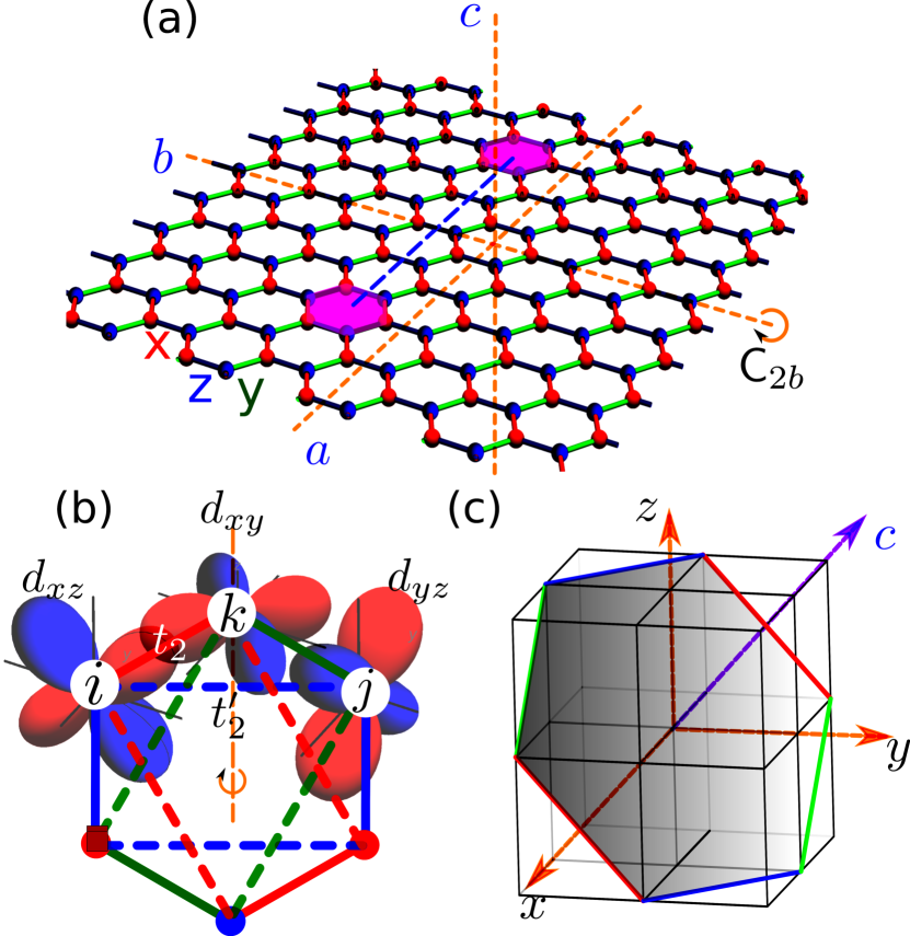
Figure 1: (a) Schematic of a finite size ($L\times L$) honeycomb lattice made out of magnetic ions with two $\mathbb{Z}_{2}$ vortices (vison excitations) [shaded region]. The vison excitations are separated by a string operator (dashed blue line) which flips $u_{ij}$ eigenvalue when it crosses a particular bond $\braket{ij}$. The colored bonds represent three anisotropic bond-dependent Kitaev interactions. The $\pi$-rotation symmetry along the crystalline axes $b$ is illustrated by the dashed orange lines. There is an additional three-fold rotation symmetry along the crystalline $c$-axis. Note that the $\pi$-rotation along the $a$-axis is not a symmetry in the presence of ligands. As an example, the crystal symmetry for the monolayer $\alpha$-$\mathrm{RuCl_{3}}$ is P6₃/mcm which does not contain $\pi$-rotation along the $a$-axis as a symmetry. (b) A single hexagonal plaquette with the (next)- nearest neighbor hopping amplitudes ($t_{2}^{\prime}$) $t_{2}$ formed by the bond-dependent orbital overlaps. (c) The relative orientation of the honeycomb plane ($abc$-coordinate system) in panel (a) with respect to the spin quantization axes ($xyz$-coordinate system).

III Microscopic model

We start from the microscopic multiorbital description for $\alpha$-RuCl₃, however, this formalism can be suitably generalized to other Kitaev candidate materials. The electronic configuration of the transition metal (TM) ion Ru in $\alpha$-RuCl₃ is $4d^{5}$. These five electrons reside in the $t_{2\mathsf{g}}$ manifold formed by the three orbitals: $d_{xy}$, $d_{yz}$ and $d_{zx}$. The presence of strong atomic SOC Sears et al. (2015); Jackeli and Khaliullin (2009); Chaloupka et al. (2013); Winter et al. (2016, 2017); Gotfryd et al. (2017) further splits this manifold into $J_{\mathrm{eff}}=1/2$ and $J_{\mathrm{eff}}=3/2$ states. This leads to a completely filled $J_{\mathrm{eff}}=3/2$ manifold with the four electrons, and the remaining electron resides in the $J_{\mathrm{eff}}=1/2$ sector. Consequently, it leads to an effective one-hole model, constructed with the following parameters: an on-site Coulomb repulsion of strength $U$, the Hund’s coupling $J_{\mathrm{H}}$, and (next-)nearest neighbor hopping ($t_{2}^{\prime}$) $t_{2}$, respectively Jackeli and Khaliullin (2009); Rau et al. (2014) [see Fig. 1(a,b)].

In the strong-coupling limit ($t_{2},t_{2}^{\prime}\ll U,J_{\mathrm{H}}$), the low-energy effective Hamiltonian is obtained by the (SWT) [see supplemental material (SM)sup for more details] and leads to the ferromagnetic Kitaev Hamiltonian as

$$\mathcal{H}_{0}=-K\sum_{\langle ij\rangle;\alpha}S^{\alpha}_{i}S^{\alpha}_{j},\quad K=\frac{8J_{\mathrm{H}}t_{2}^{2}}{3(U^{2}-4UJ_{\mathrm{H}}+3J_{\mathrm{H}}^{2})},$$ (4)

where $\langle ij\rangle$ denotes the nearest-neighbor sites, and $\alpha\in\{x,y,z\}$ labels the planar orientation of the bond-type as illustrated in Fig. 1(a)-(b). The Kitaev coupling $K$ in Eq. (4) is obtained to the lowest order in perturbation, and does not include $t_{2}^{\prime}$. Note that we treat $t_{2}^{\prime}$ as a small perturbation. We first obtain the ground state configuration without $t_{2}^{\prime}$. Then the induced orbital current is obtained by considering $t_{2}\textquoteright$ as a small perturbation, which is accurate up to the first order in $t_{2}\textquoteright$.

This model can be solved exactly, as shown by Kitaev himself Kitaev (2006), by introducing Majorana representation of the spin-1/2 operators as $S_{i}^{\alpha}=ib_{i}^{\alpha}c_{i}/2$ for $\alpha=x,y,z$. Here $b^{\alpha}_{i},c_{i}$ are four mutually anti-commuting Majorana operators. In terms of $b^{\alpha}_{i}$ and $c_{i}$, the Hamiltonian in Eq. (4) can be rewritten as $\mathcal{H}_{0}=iK/4\sum_{\langle ij\rangle}u_{ij}c_{i}c_{j}$, where $u_{ij}(=ib^{\alpha}_{i}b^{\alpha}_{j})$ are the $\mathbb{Z}_{2}$ gauge field operators with eigenvalues $\pm 1$. Since $u_{ij}$ commutes with the Hamiltonian, one can pick a particular choice of $u_{ij}$ (a gauge sector $\ket{\mathcal{G}}$) and solve the remaining non-interacting Majorana Hamiltonian. The pinned flux in each honeycomb plaquette is obtained by the gauge-invariant loop operator $\mathcal{W}_{p}=\prod_{\braket{ik}\in\mathord{\raisebox{-0.5pt}{ \leavevmode\hbox to4.21pt{\vbox to3.7pt{\text{[drawing]}}}}}_{p}}u_{ik}$. Here $\mathcal{W}_{p}=+1$ corresponds to zero-flux in a plaquette, whereas $\mathcal{W}_{p}=-1$ signifies a $\pi$-flux and corresponds to a $\mathbb{Z}_{2}$ vortex or a vison excitation [see the shaded hexagons in Fig. 1(a)]. Following Lieb’s theorem Lieb (1994), the ground state of the Majorana fermions is obtained with the gauge choice of $\mathcal{W}_{p}=1,\forall p$, for all the hexagonal plaquettes. Starting from a uniform gauge configuration, one may create a single vison excitation by changing the eigenvalue of a single plaquette loop operator to $-1$.

To induce orbital magnetization, it is necessary to break the related symmetries. In crystals realizing the Kitaev model, the symmetry is low because of the spin-orbit coupling. As shown in Fig. 1(a), the system has translation symmetry, two-fold rotation symmetry along crystalline $b$-axis denoted by $\mathsf{C}_{2b}$ in panel (a), 3-fold rotation symmetry along the $c$ axis, $\mathsf{C}_{3c}$, time-reversal symmetry (TRS) and inversion symmetry. The seemingly two-fold rotation along the $a$-axis Fig. 1(a) is absent when one embeds the honeycomb plane into the parent crystal. To allow for orbital magnetization along the $c$ axis, we need to break the TRS and also the $\mathsf{C}_{2b}$ symmetry. This can be achieved by applying a magnetic field with non-zero component perpendicular to the $b$ axis. One particularly interesting case is when the magnetic field is applied in the $a$-$b$ plane, which induces orbital magnetization along the $c$ axis. Generally, the induced magnetization is much weaker than the applied magnetic field. The case with an external magnetic field in the plane may be more convenient for experimental detection of the induced orbital magnetization.

IV Circulating loop currents

Since the parent compound of a Kitaev spin liquid is a multiorbital spin-orbit coupled Mott insulator, there is remnant charge response and there can exist localized circulating electrical currents. The charge response is governed by the charge excitation gap, which is of the order of $U$. Similar to the derivation of the effective spin Hamiltonian in Eq. (4) from the Hubbard model, we perform a strong-coupling expansion (SWT) for the current operator defined on the bond $\langle ij\rangle$ [see Fig. 1(b)] as

$$\bm{\mathcal{I}}_{ij}=\frac{iet_{2}^{\prime}\hat{\mathbf{r}}_{ij}}{\hbar}\sum_{\alpha,\beta,\sigma}\left(d^{\dagger}_{j\alpha\sigma}d_{i\beta\sigma}-d^{\dagger}_{i\beta\sigma}d_{j\alpha\sigma}\right),$$ (5)

where $d^{\dagger}_{i\alpha\sigma}$ creates an electron in the $i$-th site with spin $\sigma$ and orbital $\alpha,\beta\in\{x,y,z\}$, and obtain a generalization of Eq. (1) for the triangular loop current as (see the details of the derivation in Sec. (II) in the SM sup )

$$\tilde{\bm{\mathcal{I}}}_{ij,k} =\bm{\mathcal{I}}_{0}(3S^{x}_{i}S^{y}_{j}+S^{y}_{i}S^{x}_{j})S^{z}_{k}+$$

$$\quad\quad\bm{\mathcal{I}}_{0}(3S^{y}_{i}S^{z}_{j}-5S^{z}_{i}S^{y}_{j})S^{x}_{k}+$$

$$\quad\quad\quad\bm{\mathcal{I}}_{0}(3S^{z}_{i}S^{x}_{j}-5S^{x}_{i}S^{z}_{j})S^{y}_{k},$$ (6a)

$$\bm{\mathcal{I}}_{0} =\frac{e\hat{\mathbf{r}}_{ij}}{\hbar}\frac{8t_{2}^{2}t_{2}^{\prime}J_{\mathrm{H}}(U-2J_{\mathrm{H}})}{9(U^{2}-4UJ_{\mathrm{H}}+3J_{\mathrm{H}}^{2})^{2}},$$ (6b)

where $S^{\alpha}_{i}$ is the $\alpha$-th component of the spin at site $i$, and $U,J_{\mathrm{H}}$, and $t_{2}$ are the microscopic parameters as defined earlier. For the current operator defined on the other bonds, we need to modify the loop current expression by permuting both the orbital and site indices on the three spin operators. The expression (6a) is consistent with the $\mathsf{C}_{2b}$ symmetry [orange dashed line in Fig. 1 (b)]. Under $\mathsf{C}_{2b}$, $i\leftrightarrow j$, $k\leftrightarrow k$, $S^{x}\rightarrow-S^{y}$, $S^{y}\rightarrow-S^{x}$, $S^{z}\rightarrow-S^{z}$ and $\tilde{\bm{\mathcal{I}}}_{ij,k}=-\tilde{\bm{\mathcal{I}}}_{ji,k}$. However, the $\mathsf{C}_{2b}$ symmetry cannot uniquely determine the form of $\tilde{\bm{\mathcal{I}}}_{ij,k}$. Actually the absence of any terms with repeated index in the spin space (i.e. $S_{i}^{x}S_{j}^{x}S_{k}^{z}$) in Eq. (6a) is an artifact of considering an ideal situation, where we retain only $t_{2}$, and $t_{2}^{\prime}$ hoppings in the multiorbital tight-binding (TB) description. Indeed, a more realistic TB modeling Rau et al. (2014) for Kitaev quantum magnets would lead to additional three-spin terms with possible repeated indices. However, for the subsequent analysis in this work, we focus on the ideal Kitaev limit.

For an estimate of the amplitude of the induced electrical current, we adopt all the parameters entering Eq. (6b) from the recent ab initio Kim and Kee (2016) and photoemission reports Sinn et al. (2016) for $\alpha$-RuCl₃ as $U=3.0$ eV, $J_{\mathrm{H}}=0.45$ eV, $t_{2}=0.191$ eV, and $t^{\prime}_{2}=-0.058$ eV. The value of $t^{\prime}_{2}$ has been adopted from Ref. Eichstaedt et al. (2019). Plugging in the numbers in Eqs. (4) and (6b), we estimate $|\bm{\mathcal{I}}_{0}|\sim 30$ nA, with a Kitaev coupling $K\sim 0.023$ eV.

The key quantity now is the expectation value of the induced loop current operator in the ground state of the Kitaev model. The pure Kitaev model can be solved exactly from the Hamiltonian $\mathcal{H}_{0}=iK/4\sum_{ij}c_{i}c_{j}$, with all $u_{ij}$ chosen to be $+1$. The ground state eigenfunction can be written as $\ket{\Psi_{0}}=\mathcal{Z}\ket{\mathcal{G}_{0}}\otimes\ket{\mathcal{M}}$ where $\ket{\mathcal{G}_{0}}$ corresponds to $\mathcal{W}_{p}=1$ for all hexagonal plaquettes and $\ket{\mathcal{M}}$ is the ground state of gapless Majorana fermions sup . However as the Hilbert space is enlarged due to the fractionalization of the spin degrees of freedom, we need to project the eigenstates of $\mathcal{H}_{0}$ to the physical Hilbert space of the spin Hamiltonian in Eq. (4). The corresponding projection is achieved by the local constraint $\mathcal{D}_{i}=ic_{i}b_{i}^{x}b_{i}^{y}b_{i}^{z}=1$ and the global projection operator $\mathcal{Z}=\Pi_{i}(1+\mathcal{D}_{i})/2$ Kitaev (2006); Pedrocchi et al. (2011); Zschocke and Vojta (2015).

Due to the static nature of the vison excitations in a pure Kitaev model, only the first term, $S_{i}^{x}S_{j}^{y}S_{k}^{z}$, in Eq. (6a) contributes to the computation of the loop current expectation value in the Kitaev ground state. All the other five terms in Eq. (6a) do not contribute as they have zero expectation value in $\ket{\Psi_{0}}$ (see the SM sup for more details). It is straightforward to see that the loop current expectation value vanishes in the pure Kitaev model ground state, i.e., $\braket{\Psi_{0}}{\tilde{\bm{\mathcal{I}}}_{ij,k}}{\Psi_{0}}=0$. This absence is not a surprise, since any finite loop current would lead to an orbital magnetization that breaks TRS, whereas the ground state $\ket{\Psi_{0}}$ preserves the TRS.

IV.1 External magnetic field

The TRS of the system is broken in the presence of an external magnetic field. In this case, we may expect a finite loop current expectation value in the ground state. We consider the Kitaev model in an external magnetic field and explore its consequences. The integrability of the model is destroyed in the presence of an external magnetic field $\mathbf{h}=(\mathrm{h}_{x},\mathrm{h}_{y},\mathrm{h}_{z})$, defined along spin quantization axes (we call it the $xyz$-coordinate system). For a small $|\mathbf{h}|$, we can treat the effect of $\mathbf{h}$ in a perturbative manner. The lowest order perturbation correction, that breaks the TRS Kitaev (2006), reads as $\mathcal{H}_{\mathrm{eff}}=-\kappa\sum_{ijk,\triangle}S^{x}_{i}S^{y}_{j}S^{z}_{k}$, where $\kappa=\mathrm{h}_{x}\mathrm{h}_{y}\mathrm{h}_{z}/K^{2}$. Note that $\mathcal{H}_{\mathrm{eff}}$ has the same form as the first term in $\tilde{\bm{\mathcal{I}}}_{ij,k}$, and therefore it is natural to have a nonzero current in the QSL. Choosing the same gauge configuration $\ket{\mathcal{G}_{0}}$ as before, the total Hamiltonian $\mathcal{H}=\mathcal{H}_{0}+\mathcal{H}_{\mathrm{eff}}$ can be simplified as

$$\mathcal{H}=\frac{iK}{4}\sum_{\langle ik\rangle}c_{i}c_{k}+\frac{i\kappa}{8}\sum_{\llangle ij\rrangle}c_{i}c_{j},$$ (7)

where all the $u_{ij}$’s are replaced by their eigenvalues. The ground state eigenfunction of the above Hamiltonian can be written as $\ket{\Psi_{\mathrm{mag}}}=\mathcal{Z}\ket{\mathcal{G}_{0}}\otimes\ket{\mathcal{M}_{\mathrm{mag}}}$, where $\ket{\mathcal{M}_{\mathrm{mag}}}$ is the ground state of the gapped Majorana fermions sup , and $\mathcal{Z}$ is the global projection operator, as defined earlier. The loop current expectation value becomes non-vanishing in this case and $\braket{\Psi_{\mathrm{mag}}}{\tilde{\bm{\mathcal{I}}}_{ij,k}}{\Psi_{\mathrm{mag}}}\propto\kappa$ for $\kappa\ll K$ (see the SM sup for more details).

One key feature of the Kitaev system is that even an in-plane magnetic field [applied in the $ab$-plane shown in Fig. 1(b)] can have non-zero components along all the three spin quantization axes. Let us write the external magnetic field $\mathbf{h}^{\mathrm{ext}}$ in the coordinate system containing the honeycomb plane (we call it the $abc$-coordinate system) as $\mathbf{h}^{\mathrm{ext}}=\mathrm{h}(\sin\theta\cos\phi,\sin\theta\sin\phi,\cos\theta)$, where $\phi$ and $\theta$ are azimuthal angle measured from the crystalline $a$ axis and polar angle from the crystalline $c$ axis, respectively, and $\mathrm{h}$ is the strength of the applied magnetic field. After a straightforward transformation between the $abc$- and the $xyz$-coordinate system [see Fig. 1(c)], we obtain sup

$$(\mathrm{h}_{x},\mathrm{h}_{y},\mathrm{h}_{z})=\mathrm{h}\left(\frac{\cos\theta}{\sqrt{3}}+\frac{\sin\theta\cos\phi}{\sqrt{6}}-\frac{\sin\theta\sin\phi}{\sqrt{2}},\;\frac{\cos\theta}{\sqrt{3}}+\frac{\sin\theta\cos\phi}{\sqrt{6}}+\frac{\sin\theta\sin\phi}{\sqrt{2}},\;\frac{\cos\theta}{\sqrt{3}}-\sqrt{\frac{2}{3}}\sin\theta\cos\phi\right).$$ (8)

It is evident from Eq. (8) that even for an in-plane magnetic field (with $\theta=0$), one can have non-zero $(\mathrm{h}_{x},\mathrm{h}_{y},\mathrm{h}_{z})$, leading to a finite $\kappa$. By rotating the magnetic field in the $ab$-plane, $\kappa$ can change the sign and even become zero for certain angles (see the SM sup for the details about the variation of $\kappa$ as a function of this rotation angle). For the field applied along the $b$ axis, $\theta=\pi/2$ and $\phi=\pi/2$, we have $\kappa=0$ and therefore the induced orbital magnetization vanishes, which is consistent with the symmetry analysis above.

When the magnetic field strength becomes large, the perturbative treatment is inadequate. In addition to the $\kappa$ term, the magnetic field generates dynamics for the visons, which spoil the integrability of the model. To make analytical progress, we take $\kappa$ as a free parameter with the understanding that it relates to the magnetic field for a weak field. The main results of the orbital magnetization obtained below are expected to hold even when visons are dynamical. For a large magnetic field, the chiral Kiteav QSL is destroyed and the description in Eq. (7) is no longer applicable Patel and Trivedi (2019); Hickey and Trebst (2019).

So far we focused on a specific triangular plaquette, however, in a lattice geometry, the situation becomes more interesting. A specific triangle is shared between three honeycomb plaquettes, whereas each nearest-neighbor (NN) bond on the triangle is shared between four triangles. Among these four triangles, two belong to the hexagonal plaquette containing the next-nearest neighbor (NNN) bond $\langle ij\rangle$, where the current operator is defined, and the other two belong to the neighboring hexagonal plaquettes (see Fig. 1). Consequently, the net current along the NN bonds forming the honeycomb plaquettes vanishes because of counter-propagating currents from the two honeycomb plaquettes for translationally invariant systems. In a finite size system with open boundary conditions (OBC), however, such perfect cancellations are not possible near the edge terminations, as shown in Fig. 2. On the other hand, since the NNN bonds are not shared between any plaquettes, the localized currents are never canceled and they create an interesting loop current profile distributed over the entire system, as will be discussed in the next section.

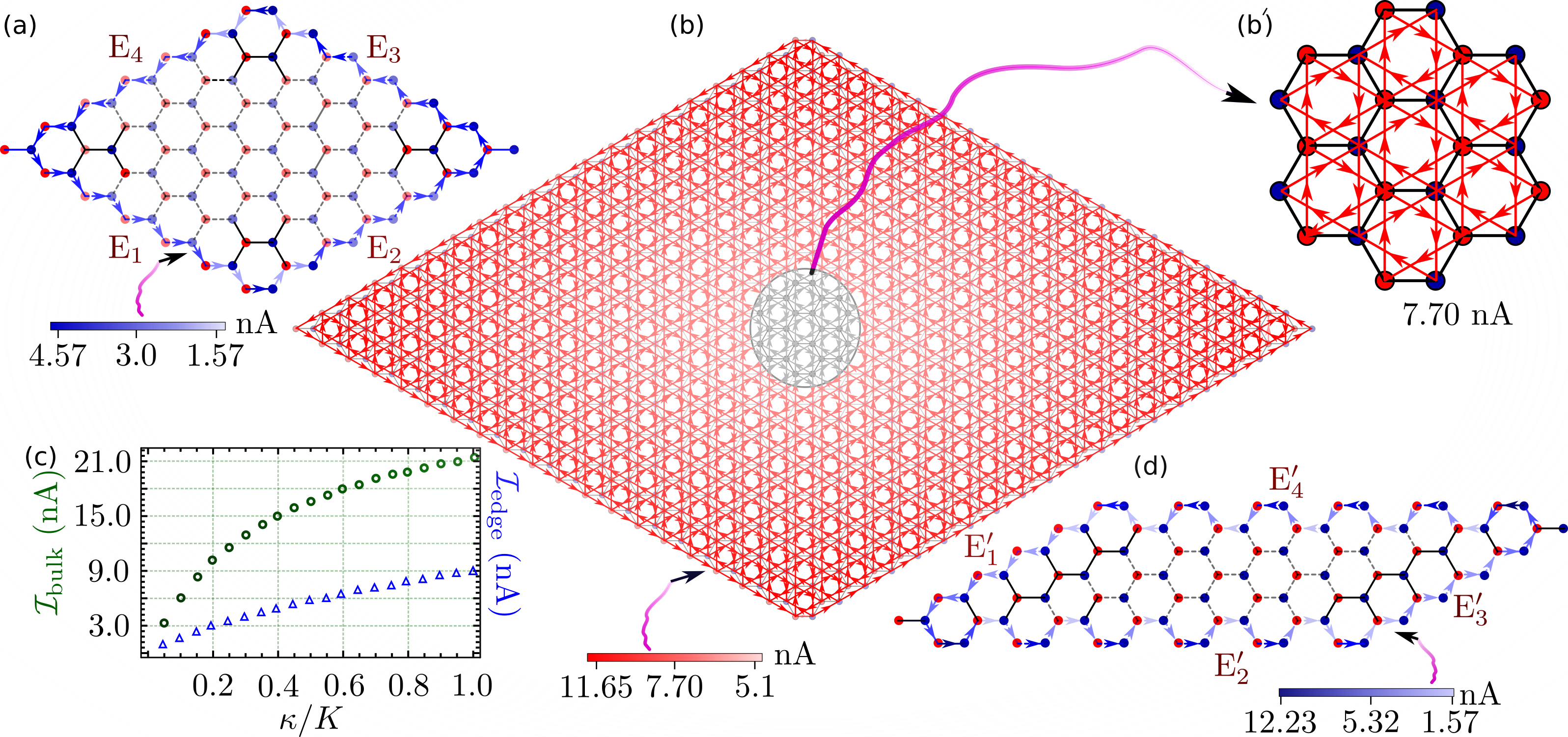
Figure 2: (a) Distribution of the localized edge currents around the zigzag type edges for a finite system with OBC of size $L=21$ (the bulk of the system is illustrated by the dashed bonds). Note that the localized currents on four different edges are displayed only for the bonds lying on the honeycomb plaquettes. The localized currents on the next-nearest neighbor (NNN) bonds are not shown for simplicity. (b) The macroscopic build-up of localized currents along the NNN bonds is distributed over the entire sample size and forms filament-like current textures. A magnified view of the details of the current textures in the middle of the system is shown in the top right panel (b^′). (c) The variation of the localized current as a function of $\kappa$ for the nearest-neighbor (NN) bonds on the middle of the edges $\mathrm{E}_{1}-\mathrm{E}_{4}$ (open triangles) and NNN bonds inside the lattice (open circles), respectively. (d) The current profile around a different geometry with both the zigzag and arm-chair edges. The numerical estimates are provided with $\kappa=0.2K$.

V Finite system analysis

We now focus our analysis on a finite system to compute the localized current profile. We first consider a finite system (with OBC) of linear size $L$ without any $\mathbb{Z}_{2}$ vortices or vison excitations. We set the value of $\kappa$ motivated by the recent experimental work on $\alpha$-RuCl₃ Tanaka et al. (2022). Comparing the gap magnitude from Eq. (7) with the observed field-dependent Majorana gap at an applied magnetic field of $\sim 10$ T, we estimate $\kappa\sim 0.77K$. However, this value of $\kappa$ corresponds to a large magnetic field, when our approximate Hamiltonian in Eq. (7) is no longer applicable. Hence, we use a smaller magnitude of $\kappa=0.2K$ for subsequent quantitative estimates, unless otherwise mentioned. As explained previously, the localized current on a particular bond $\braket{ij}_{\alpha}$ on the honeycomb plaquette is the sum of the contributions from the associated triangles. Following the analytical form in Eq. (6a), it appears as if there are three different average currents $\mathcal{I}_{\alpha}$ in three different bonds, $\alpha=x,y,z$, respectively [see Fig. 1(a)]. However, the $C_{3}$ rotation symmetry of the underlying lattice implies that all these three currents are identical i.e., $\mathcal{I}_{\alpha}=\mathcal{I}$. In addition, neighboring honeycomb plaquettes of a particular bond host counter-propagating current $\mathcal{I}$, leading to vanishing average current distribution at the sides of each honeycomb plaquette in the bulk. However, such perfect cancellations are absent near the edge terminations of the finite system, which consequently leads to non-vanishing localized currents around the edge as shown in Fig. 2(a) and 2(c). The lack of translational invariance around the edges of the system leads to different localized currents along different bonds in each of the triangular plaquettes along the edge. The total current is conserved at each vertex.

On the other hand, the localized currents in each of the NNN bonds $\braket{ij}$ within the triangle $\triangle_{ijk}$ do not vanish as they are not shared between other triangles in the lattice geometry. It leads to a macroscopic build-up of the localized currents which mimics a filament like structure distributed over the entire system, as shown in Fig. 2(b). For an infinite system, these localized currents on the NNN bonds, form an emergent superlattice of two interpenetrating triangular lattices as illustrated in Fig. 2(b^′). We emphasize that there is no free-flowing current over long distances because of the Mott nature of the system. Currents only flow around a closed loop of atomic size. The seemingly free flow of current (red line in Fig. 2(b)) is an illusion due to the superposition of localized current loops. The dependence of the current amplitude as a function of $\kappa$ is shown in Fig. 2(c). In the subsequent sections Sec. V.1, and  V.2, we focus on two types of edge-termination geometry for finite systems with OBC in the absence of vison excitations. In Sec. V.3, we again consider a finite system with PBC in the presence of two well-separated $\mathbb{Z}_{2}$ vortices, and illustrate the drastic modification of the bulk loop currents around these vison excitations.

V.1 Quantitative estimates and analysis – case of zigzag geometry

We performed numerical diagonalization for a system of linear size $L=21$ with zigzag edge terminations to obtain the average localized current distribution without any vison excitations. In this case, the thermodynamic limit is reached for a relative small system size $L\geq 20$ because the system is fully gapped. (see the SM  sup for the technical details). The corresponding results are shown in Fig. 2(a-c). In this geometry, the four different zigzag edges $\mathrm{E}_{1}-\mathrm{E}_{4}$ are related to each other by the three-fold rotation along the $c$-axis, and we focus on one edge viz. $\mathrm{E}_{1}$ for the quantitative analysis.

As shown in Fig. 2(a), the edge $\mathrm{E}_{1}$ is formed by two types of bonds: $x$- and $z$-bond. In the thermodynamic limit, we obtain a localized current that saturates at $\mathcal{I}^{(0)}_{\mathrm{edge}}\sim 3.0$ nA for both the bonds, that lie far away from the corner sites with $\mathrm{E}_{2}$ and $\mathrm{E}_{4}$, respectively. The variation of the the thermodynamic edge current $\mathcal{I}^{(0)}_{\mathrm{edge}}$ as a function of $\kappa$ is shown in Fig. 2(c) (see the variation with open triangles).

The value of $\mathcal{I}_{\mathrm{edge}}$ deviates toward the corners of the system and differs for each bond type because of the lack of translation invariance along the edge. The amplitude for $z(x)$-bond near the corner with $\mathrm{E}_{4}$ is $\sim 4.57$ ($3.83$) nA, whereas near the other corner with $\mathrm{E}_{2}$ it is slightly less $\sim 2.21$ ($1.58$) nA as shown in Fig. 2(a). This variation along the edge is illustrated by the color legend below panel (a) in Fig. 2. The saturation length (the distance beyond which the bond currents become $\mathcal{I}^{(0)}_{\mathrm{edge}}$) near the edge with $\mathrm{E}_{4}$ is slightly larger than the saturation length near the edge with $\mathrm{E}_{2}$. Furthermore, the currents on the NN bonds inside the system almost vanish as mentioned earlier.

On the other hand, the current amplitude on the NNN bonds [$x^{\prime},y^{\prime},z^{\prime}$-type corresponding to $t_{2}^{\prime}$ hopping, see Fig. 1(b)] inside the lattice far away from the edges and corners saturates at $\mathcal{I}^{(0)}_{\mathrm{bulk}}\sim 7.70$ nA as shown in Fig. 2(b). In comparison to the edge current $\mathcal{I}^{(0)}_{\mathrm{edge}}$, the variation of this thermodynamic bulk localized current $\mathcal{I}^{(0)}_{\mathrm{bulk}}$ as a function of $\kappa$ is shown in Fig. 2(c) (see the variation with open circles). This value also deviates from the bulk value as the bonds come close to the edges/corners of the system. The $\mathsf{C}_{3c}$ rotation symmetry, which enforces identical localized currents $\mathcal{I}^{(0)}_{\mathrm{bulk}}$ on all $x^{\prime},y^{\prime},z^{\prime}$ bonds in the bulk, is lost as we go away from the middle of the system to its edge. Consequently, the amplitudes of the localized currents for the three bonds gradually differ as they come closer to the edge/corner as illustrated by the color legend below panel (b) in Fig. 2.

V.2 Quantitative estimates and analysis – case of armchair geometry

In the previous section, we focused our quantitative analysis on a finite-size honeycomb lattice with zigzag edges as shown in Fig. 2(a). However, such edge terminations are not the only possible options. Motivated by the graphene literature Castro Neto et al. (2009); Wimmer et al. (2010); Nakada et al. (1996), we consider a different geometry with both the zigzag and the armchair edge terminations, as shown in Fig. 2(d). Such geometry can be created by modifying the choice of the unit vectors Kohmoto and Hasegawa (2007) compared to the previous case. We again perform numerical diagonalization on this geometry of linear size $L=21$ to obtain the current distribution, without any vison excitations. The localized current on the NNN bonds in the middle of the system saturates at the same value $\mathcal{I}^{(0)}_{\mathrm{bulk}}$ as before. There are four edges and two pairs of edges are related by the inversion operation. Consequently, we focus only on two different edges $\mathrm{E}^{\prime}_{1}$ and $\mathrm{E}^{\prime}_{2}$ with zigzag and armchair termination, respectively. For $\mathrm{E}^{\prime}_{1}$ (with $z$ and $y$-bonds), the current far away from the corners saturates at the same amplitude $\mathcal{I}^{(0)}_{\mathrm{edge}}$ as quoted in the previous section. Of course, this number varies as the bonds come close to the corners as before. This variation is similar to Fig. 2(a).

However, the localized current distribution along the armchair edge $\mathrm{E}^{\prime}_{2}$ (with all the three bonds – $x$, $y$ and $z$) is very different from its zigzag counterpart. The amplitude of the current on the outer lying $z$-bonds in the middle of the edge, away from the corners, saturates at a larger value $\mathcal{I}^{(0)}_{\mathrm{z-ach}}\sim 10.35$ nA, whereas the current on the accompanying $x$ and $y$-bonds saturates at a lower value $\mathcal{I}^{(0)}_{\mathrm{xy-ach}}\sim 4.31$ nA. The variation of the localized currents on the bonds as they come close to the corners for both the zigzag and the armchair edge terminations is illustrated in Fig. 2(d). The current profile on the NNN bonds is similar to the previous case and is not shown for simplicity. A more interesting edge current profile can be obtained by modifying the edge termination patterns to others such as the bearded edge ribbons Kohmoto and Hasegawa (2007).

V.3 Quantitative estimates and analysis – case of two vison excitations

In this section, we analyze the current distributions in the presence of localized vison excitations. For this purpose, we now consider a finite system with PBC and a bigger linear size $L=32$ compared to the previous case. We chose a bigger system size to reduce the mutual interaction between the two vison excitations.

We introduce two visons and keep them at the largest possible distance $\lfloor\tfrac{L-1}{2}\rfloor$ to minimize their mutual interaction effects. Such configuration can be achieved by flipping all the link variables on the $z$-bonds which are connected by the string operator between them, as illustrated in Fig. 1(a). However, as the string operator is gauge-dependent, the specific choice of the string operator connecting two vison excitations does not affect the electrical currents.

The ground state of the two-vison Kitaev model, in the presence of an external magnetic field can be similarly obtained, utilizing the Majorana and gauge degrees of freedom, as $\ket{\Psi^{(2)}_{\mathrm{mag}}}=\mathcal{Z}\ket{\mathcal{G}_{2}}\otimes\ket{\mathcal{M}_{\mathrm{mag}}}$. Here $\ket{\mathcal{G}_{2}}$ corresponds to the gauge configuration with two visons, and $\mathcal{Z}$ is the projection operator as defined in Sec. (IV). We note that the action of the projection operator $\mathcal{Z}$ translates into satisfying a parity constraint for the matter and bond fermions as $(-1)^{n_{f}+n_{\chi}}=1$ (see the SM sup for the technical details) Zschocke and Vojta (2015); Pedrocchi et al. (2011). Next, we compute the average localized current in the ground state $\ket{\Psi^{(2)}_{\mathrm{mag}}}$, by numerically diagonalizing the tight-binding Majorana Hamiltonian with $\ket{\mathcal{G}_{2}}$ sup .

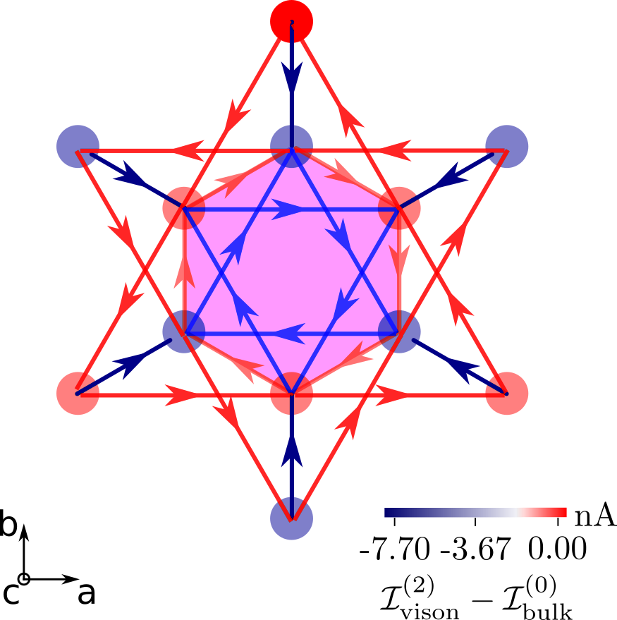
Figure 3: Current profile around a vison excitation (colored hexagon). In contrast to the previous case in Fig. 2, the localized currents on the NN bonds around honeycomb plaquettes containing the vison are nonzero.

In the previous section with the gauge configuration $\ket{\mathcal{G}_{0}}$, we observed that the localized currents on the NNN bonds, within the bulk, saturated at a uniform value $\mathcal{I}^{(0)}_{\mathrm{bulk}}$. Such current configuration led to vanishing localized currents on the NN bonds forming the hexagonal plaquettes. In the case with the gauge configuration $\ket{\mathcal{G}_{2}}$, the localized current profile far away from the static vison excitations is identical to $\mathcal{I}^{(0)}_{\mathrm{bulk}}$.

However, this distribution acquires drastic modification inside and around the vison excitations. The localized currents on the three NNN bonds ($x^{\prime}$, $y^{\prime}$, and $z^{\prime}$-bonds) within the hexagon containing a vison excitation become isotropic but differ from the localized currents on the NNN bonds surrounding the honeycomb plaquettes, and consequently, finite non-vanishing currents emerge on the NN bonds forming the hexagon, as shown in Fig. 3. The localized current on the NNN bonds inside the vison $\mathcal{I}^{(2)}_{\mathrm{vison}}$ saturate at a smaller value of $\sim 4.03$ nA, whereas the corresponding currents on the surrounding hexagons saturates at almost $\mathcal{I}^{(0)}_{\mathrm{bulk}}\sim 7.70$ nA. Consequently, NN bonds surrounding the hexagon containing the vison excitation host non-zero localized loop currents $\mathcal{I}^{(2)}_{\mathrm{vison-edge}}\sim 7.29$ nA, which is obtained by adding the contributions of the four triangular plaquettes containing the NN bonds. The variation of the amplitudes of these localized currents on the vison plaquettes as a function of the orientation and magnitude of the external magnetic field follows similar dependence as was illustrated in Fig. 2(c) in Sec. (V).

VI Loop currents: Implications

So far, we discussed patterns of the TRS breaking localized loop currents in a Kitaev system in the presence of an external magnetic field. For an infinite system, we noticed that the localized loop currents constitute a superlattice formed by inter-penetrating triangular lattices as shown in Fig. 2(b^′). The direction of the loop currents is determined by the sign of $\kappa$ and therefore depends on the direction of the external magnetic field. Therefore, in the absence of any vison excitations, one should expect them to contribute a uniform local magnetic moment $\mu_{\mathrm{loop}}$ for each of the hexagonal plaquettes. Since the current orientation for both the triangular plaquettes is the same, the magnetic moment of each of the two triangles adds up and leads to a total orbital magnetic moment in each hexagon as $\mu_{\mathrm{hexagon}}=2\times\mu_{\mathrm{loop}}$. Adopting realistic atomic lattice constant for $\alpha$-RuCl₃ from the recent ab intio study Kim and Kee (2016), we obtain $\mu_{\mathrm{hexagon}}\sim 0.0003\mu_{\mathrm{B}}$, where $\mu_{\mathrm{B}}$ is the Bohr-magneton. Consequently, we find a weak emergent orbital ferromagnetic magnetic order within the Kitaev QSL phase. Naturally, the vison excitations would create a local change in this emergent long-range orbital ferromagnetic phase as the localized currents are different around the vison excitations. Adopting the previous parameters, we estimate that the magnitude of the local magnetization on an isolated vison to be $\sim\pm 20\%$ of the $\mu_{\rm{hexagon}}$. Such orbital ferromagnetic order can be resolved by polarized neutron diffraction Fauqué et al. (2006); Jeong et al. (2017), muon spin spectroscopy Zhang et al. (2018), second harmonic generation Zhao et al. (2016), optical birefringence measurements Lubashevsky et al. (2014), or superconducting quantum interference device magnetometers Lampen-Kelley et al. (2018).

The key feature of the Kitaev system is that for an external magnetic field only applied in $ab$-plane would lead to an induced out-of-plane (along $c$-axis) magnetization. The direction and the magnitude of such $c$-axis magnetic field can be tuned by rotating the magnetic field in the $ab$-plane. Note that the direction of the orbital magnetic field depends on the sign of $\kappa$ which is dictated by Eq. (8).

The magnitude of the localized moments is weak based on our quantitative estimate for $\alpha$-RuCl₃. However, two polymorphs of $\alpha$-RuCl₃, by replacing the ligand Cl^--ion with Br^- and I^-, have recently become possible candidate materials for realizing Kitaev QSL phase Kaib et al. (2022). Among these two polymorphs, RuI₃ is still debated to be a metal, although RuBr₃ is an insulator with almost half the Mott gap compared to RuCl₃ Kaib et al. (2022). On the other hand, it has a much larger Ru-Ru distance and considerable Ru 4$d$ and Br 4$p$ orbital overlap Imai et al. (2022). Adopting the parameters from the ab initio Ersan et al. (2019) results for RuBr₃, we predict an order of magnitude enhancement of such localized magnetic moments for an analogous situation in RuBr₃ with $\mu_{\mathrm{hexagon}}\sim 0.003\mu_{\mathrm{B}}$ at $\kappa\sim 0.14K$ if the Kitaev quantum spin liquid phase can be realized there. On the other hand, if we adopt an inflated magnitude of $\kappa$ for RuBr₃ motivated by the experimentally measured Majorana gap for $\alpha$-RuCl₃ Tanaka et al. (2022) as $\kappa\sim 0.77$, the orbital magnetization can go up as much as $0.01\mu_{\mathrm{B}}$.

VII Discussion and conclusion

In this paper, we developed a theoretical framework for analyzing the remnant electrical current responses in spin-orbit coupled multiorbital Mott insulators, such as iridates or ruthenates, considered to be plausible candidate materials to realize the Kitaev QSL phase. Our analysis and predictions reveal an exciting and alternative detection protocol for the signatures of the fractionalized excitations in a Kitaev QSL through emergent orbital magnetization due to the localized orbital currents. This formalism can be generalized to other QSL hosting Mott insulators with broken time-reversal symmetry. Starting from the microscopic multiorbital Hubbard-Kanamori model, we derived the functional form of the induced localized currents in a triangular loop [see Eq. (6a)] using SWT. The current operator expressed in terms of the spin operator in Mott insulators without SU(2) spin rotation symmetry is an important result, on its own, and forms the basis for the rest of our paper. In the presence of an external magnetic field, we solve the Kitaev model in the Majorana representation and notice that the ground state hosts a non-zero expectation value for the localized loop currents. Because of the underlying honeycomb lattice structure, the average non-zero triangular loop current leads to a rich current profile in the two-dimensional system, as shown in Fig. 2. The current on the NNN bonds on the hexagonal plaquettes extends over the entire system and forms a super-lattice of two inter-penetrating triangular lattices as illustrated in Fig. 2(b^′), whereas the current on the NN bonds vanishes identically within the bulk. However, depending on the edge termination profiles (zigzag, armchair, or bearded) of the 2D Kitaev system, the localized currents on the NN bonds along the edge can survive and lead to rich and interesting patterns.

We then revisited the analysis of our current profile in the presence of vison excitations. While the localized current distribution in the absence of any visons (uniform gauge configuration) remains identical on the NNN bonds within the bulk, leading to the vanishing currents on NN bonds, a single vison excitation leads to a drastic modification of the currents on the bonds containing the $\mathbb{Z}_{2}$ vortex (see Fig. 3). Depending on the orientation of the applied magnetic field, the currents on NNN bonds in hexagons containing the $\mathbb{Z}_{2}$ vortex decrease compared to the surrounding hexagons away from the vison excitation. This leads to a reappearance of non-zero localized currents on the NN bonds around the hexagon with vison excitation, and implies that the visons carry the physical magnetic flux, which makes visons resemble the Abrikosov vortices in superconductors. Note that the inevitable presence of local inhomogeneities in real materials would also leads to modifications of the magnetization profile because of the breakdown of translational invariance. The current pattern induced by impurities can be random and is different from the current pattern induced by a vison. Furthermore, visons are dynamical excitations of the quantum spin liquid, while the orbital current induced by impurities is static. These two distinct features for current induced by impurities and visons can be easily distinguished.

The visons can couple to an external magnetic field directly and can interact through electromagnetic coupling. This direct electromagnetic coupling is generally weak because of the small magnetic moment associated with visons. Under the circumstances when the vison gap is small, one may induce vison lattice by an external magnetic field similar to the Abrikosov vortex lattice.

VIII Acknowledgments

We would like to thank Philipp Gegenwart, Alexander V. Balatsky, Cristian Batista, Dieter Vollhardt, Krishnendu Sengupta, Ross David Mcdonald, Vivien Zapf, Avadh Saxena, and Umesh Kumar for useful discussions and careful remarks on the manuscript. This work was carried out under the auspices of the US DOE NNSA under Contract No. 89233218CNA000001 through the LDRD Program, and was performed, in part, at the Center for Integrated Nanotechnologies, an Office of Science User Facility operated for the U.S. DOE Office of Science, under user proposals $\#2018BU0010$ and $\#2018BU0083$.

References

- Balents (2010) Leon Balents, “Spin liquids in frustrated magnets,” Nature 464, 199–208 (2010).
- Savary and Balents (2016) Lucile Savary and Leon Balents, “Quantum spin liquids: a review,” Rep. Prog. Phys. 80, 016502 (2016).
- Zhou et al. (2017) Yi Zhou, Kazushi Kanoda, and Tai-Kai Ng, “Quantum spin liquid states,” Rev. Mod. Phys. 89, 025003 (2017).
- Takagi et al. (2019) Hidenori Takagi, Tomohiro Takayama, George Jackeli, Giniyat Khaliullin, and Stephen E. Nagler, “Concept and realization of Kitaev quantum spin liquids,” Nat. Rev. Phys. 1, 264–280 (2019).
- Anderson (1973) P.W. Anderson, “Resonating valence bonds: A new kind of insulator?” Mater. Res. Bull. 8, 153–160 (1973).
- Bednorz and Müller (1986) J. G. Bednorz and K. A. Müller, “Possible high Tc superconductivity in the Ba-La-Cu-O system,” Z. Phys. B Condens. Matter 64, 189–193 (1986).
- Baskaran et al. (1987) G. Baskaran, Z. Zou, and P.W. Anderson, “The resonating valence bond state and high-Tc superconductivity — A mean field theory,” Solid State Commun. 63, 973–976 (1987).
- Kalmeyer and Laughlin (1987) V. Kalmeyer and R. B. Laughlin, “Equivalence of the resonating-valence-bond and fractional quantum Hall states,” Phys. Rev. Lett. 59, 2095–2098 (1987).
- Affleck and Marston (1988) Ian Affleck and J. Brad Marston, “Large-n limit of the Heisenberg-Hubbard model: Implications for high-Tc superconductors,” Phys. Rev. B 37, 3774–3777 (1988).
- Senthil and Fisher (2000) T. Senthil and Matthew P. A. Fisher, “ gauge theory of electron fractionalization in strongly correlated systems,” Phys. Rev. B 62, 7850–7881 (2000).
- Senthil and Fisher (2001) T. Senthil and Matthew P. A. Fisher, “Fractionalization in the Cuprates: Detecting the Topological Order,” Phys. Rev. Lett. 86, 292–295 (2001).
- Kitaev (2006) Alexei Kitaev, “Anyons in an exactly solved model and beyond,” Ann. Phys. 321, 2–111 (2006).
- Singh et al. (2012) Yogesh Singh, S. Manni, J. Reuther, T. Berlijn, R. Thomale, W. Ku, S. Trebst, and P. Gegenwart, “Relevance of the Heisenberg-Kitaev Model for the Honeycomb Lattice Iridates A2IrO3,” Phys. Rev. Lett. 108, 127203 (2012).
- Banerjee et al. (2016) A. Banerjee, C. A. Bridges, J.-Q. Yan, A. A. Aczel, L. Li, M. B. Stone, G. E. Granroth, M. D. Lumsden, Y. Yiu, J. Knolle, S. Bhattacharjee, D. L. Kovrizhin, R. Moessner, D. A. Tennant, D. G. Mandrus, and S. E. Nagler, “Proximate Kitaev quantum spin liquid behaviour in a honeycomb magnet,” Nat. Mater. 15, 733–740 (2016).
- Shitade et al. (2009) Atsuo Shitade, Hosho Katsura, Jan Kunes, Xiao-Liang Qi, Shou-Cheng Zhang, and Naoto Nagaosa, “Quantum Spin Hall Effect in a Transition Metal Oxide Na2IrO3,” Phys. Rev. Lett. 102, 256403 (2009).
- Chaloupka et al. (2010) Jiri Chaloupka, George Jackeli, and Giniyat Khaliullin, “Kitaev-Heisenberg Model on a Honeycomb Lattice: Possible Exotic Phases in Iridium Oxides A2IrO3,” Phys. Rev. Lett. 105, 027204 (2010).
- Bhattacharjee et al. (2012) Subhro Bhattacharjee, Sung-Sik Lee, and Yong Baek Kim, “Spin-orbital locking, emergent pseudo-spin and magnetic order in honeycomb lattice iridates,” New J. Phys. 14, 073015 (2012).
- Rau et al. (2014) Jeffrey G. Rau, Eric Kin-Ho Lee, and Hae-Young Kee, “Generic Spin Model for the Honeycomb Iridates beyond the Kitaev Limit,” Phys. Rev. Lett. 112, 077204 (2014).
- Yadav et al. (2018) Ravi Yadav, Stephan Rachel, Liviu Hozoi, Jeroen van den Brink, and George Jackeli, “Strain- and pressure-tuned magnetic interactions in honeycomb Kitaev materials,” Phys. Rev. B (R) 98, 121107 (2018).
- Yu et al. (2013) Yue Yu, Long Liang, Qian Niu, and Shaojing Qin, “Tuning into the Kitaev spin liquid phase: A spin model on the honeycomb lattice with two types of Heisenberg exchange couplings,” Phys. Rev. B (R) 87, 041107 (2013).
- Arakawa and Yonemitsu (2021) Naoya Arakawa and Kenji Yonemitsu, “Floquet engineering of Mott insulators with strong spin-orbit coupling,” Phys. Rev. B 103, L100408 (2021).
- Strobel and Daghofer (2022) Pascal Strobel and Maria Daghofer, “Comparing the influence of Floquet dynamics in various Kitaev-Heisenberg materials,” Phys. Rev. B 105, 085144 (2022).
- Banerjee et al. (2022) Saikat Banerjee, Umesh Kumar, and Shi-Zeng Lin, “Inverse Faraday effect in Mott insulators,” Phys. Rev. B 105, L180414 (2022).
- Kumar et al. (2022) Umesh Kumar, Saikat Banerjee, and Shi-Zeng Lin, “Floquet engineering of Kitaev quantum magnets,” Commun. Phys. 5, 157 (2022).
- Baek et al. (2017) S.-H. Baek, S.-H. Do, K.-Y. Choi, Y. S. Kwon, A. U. B. Wolter, S. Nishimoto, Jeroen van den Brink, and B. Büchner, “Evidence for a Field-Induced Quantum Spin Liquid in -RuCl3,” Phys. Rev. Lett. 119, 037201 (2017).
- Sears et al. (2017) J. A. Sears, Y. Zhao, Z. Xu, J. W. Lynn, and Young-June Kim, “Phase diagram of -RuCl3 in an in-plane magnetic field,” Phys. Rev. B (R) 95, 180411 (2017).
- Wolter et al. (2017) A. U. B. Wolter, L. T. Corredor, L. Janssen, K. Nenkov, S. Schönecker, S.-H. Do, K.-Y. Choi, R. Albrecht, J. Hunger, T. Doert, M. Vojta, and B. Büchner, “Field-induced quantum criticality in the Kitaev system -RuCl3,” Phys. Rev. B (R) 96, 041405 (2017).
- Leahy et al. (2017) Ian A. Leahy, Christopher A. Pocs, Peter E. Siegfried, David Graf, S.-H. Do, Kwang-Yong Choi, B. Normand, and Minhyea Lee, “Anomalous Thermal Conductivity and Magnetic Torque Response in the Honeycomb Magnet -RuCl3,” Phys. Rev. Lett. 118, 187203 (2017).
- Banerjee et al. (2018) Arnab Banerjee, Paula Lampen-Kelley, Johannes Knolle, Christian Balz, Adam Anthony Aczel, Barry Winn, Yaohua Liu, Daniel Pajerowski, Jiaqiang Yan, Craig A. Bridges, Andrei T. Savici, Bryan C. Chakoumakos, Mark D. Lumsden, David Alan Tennant, Roderich Moessner, David G. Mandrus, and Stephen E. Nagler, “Excitations in the field-induced quantum spin liquid state of -RuCl3,” npj Quantum Mater. 3, 8 (2018).
- Hentrich et al. (2018) Richard Hentrich, Anja U. B. Wolter, Xenophon Zotos, Wolfram Brenig, Domenic Nowak, Anna Isaeva, Thomas Doert, Arnab Banerjee, Paula Lampen-Kelley, David G. Mandrus, Stephen E. Nagler, Jennifer Sears, Young-June Kim, Bernd Büchner, and Christian Hess, “Unusual Phonon Heat Transport in -RuCl3: Strong Spin-Phonon Scattering and Field-Induced Spin Gap,” Phys. Rev. Lett. 120, 117204 (2018).
- Balz et al. (2019) Christian Balz, Paula Lampen-Kelley, Arnab Banerjee, Jiaqiang Yan, Zhilun Lu, Xinzhe Hu, Swapnil M. Yadav, Yasu Takano, Yaohua Liu, D. Alan Tennant, Mark D. Lumsden, David Mandrus, and Stephen E. Nagler, “Finite field regime for a quantum spin liquid in -RuCl3,” Phys. Rev. B (R) 100, 060405 (2019).
- Czajka et al. (2021) Peter Czajka, Tong Gao, Max Hirschberger, Paula Lampen-Kelley, Arnab Banerjee, Jiaqiang Yan, David G. Mandrus, Stephen E. Nagler, and N. P. Ong, “Oscillations of the thermal conductivity in the spin-liquid state of -RuCl3,” Nat. Phys. 17, 915–919 (2021).
- Tanaka et al. (2022) O. Tanaka, Y. Mizukami, R. Harasawa, K. Hashimoto, K. Hwang, N. Kurita, H. Tanaka, S. Fujimoto, Y. Matsuda, E.-G. Moon, and T. Shibauchi, “Thermodynamic evidence for a field-angle-dependent Majorana gap in a Kitaev spin liquid,” Nat. Phys. 18, 429–435 (2022).
- Bruin et al. (2022) J. A. N. Bruin, R. R. Claus, Y. Matsumoto, N. Kurita, H. Tanaka, and H. Takagi, “Robustness of the thermal Hall effect close to half-quantization in -RuCl3,” Nat. Phys. 18, 401–405 (2022).
- Kasahara et al. (2018) Y. Kasahara, T. Ohnishi, Y. Mizukami, O. Tanaka, Sixiao Ma, K. Sugii, N. Kurita, H. Tanaka, J. Nasu, Y. Motome, T. Shibauchi, and Y. Matsuda, “Majorana quantization and half-integer thermal quantum Hall effect in a Kitaev spin liquid,” Nature 559, 227–231 (2018).
- Trebst and Hickey (2022) Simon Trebst and Ciarán Hickey, “Kitaev materials,” Phys. Rep. 950, 1–37 (2022).
- Bulaevskii et al. (2008) L. N. Bulaevskii, C. D. Batista, M. V. Mostovoy, and D. I. Khomskii, “Electronic orbital currents and polarization in Mott insulators,” Phys. Rev. B 78, 024402 (2008).
- Barkeshli et al. (2014) Maissam Barkeshli, Erez Berg, and Steven Kivelson, “Coherent transmutation of electrons into fractionalized anyons,” Science 346, 722–725 (2014).
- Pereira and Egger (2020) Rodrigo G. Pereira and Reinhold Egger, “Electrical Access to Ising Anyons in Kitaev Spin Liquids,” Phys. Rev. Lett. 125, 227202 (2020).
- Aasen et al. (2020) David Aasen, Roger S. K. Mong, Benjamin M. Hunt, David Mandrus, and Jason Alicea, “Electrical Probes of the Non-Abelian Spin Liquid in Kitaev Materials,” Phys. Rev. X 10, 031014 (2020).
- Barkeshli and Qi (2012) Maissam Barkeshli and Xiao-Liang Qi, “Topological Nematic States and Non-Abelian Lattice Dislocations,” Phys. Rev. X 2, 031013 (2012).
- Barkeshli et al. (2013) Maissam Barkeshli, Chao-Ming Jian, and Xiao-Liang Qi, “Twist defects and projective non-Abelian braiding statistics,” Phys. Rev. B 87, 045130 (2013).
- Motrunich (2006) Olexei I. Motrunich, “Orbital magnetic field effects in spin liquid with spinon Fermi sea: Possible application to -(ET)2Cu2(CN)3,” Phys. Rev. B 73, 155115 (2006).
- Kim and Kee (2016) Heung-Sik Kim and Hae-Young Kee, “Crystal structure and magnetism in RuCl3: An ab initio study,” Phys. Rev. B 93, 155143 (2016).
- Sinn et al. (2016) Soobin Sinn, Choong Hyun Kim, Beom Hyun Kim, Kyung Dong Lee, Choong Jae Won, Ji Seop Oh, Moonsup Han, Young Jun Chang, Namjung Hur, Hitoshi Sato, Byeong-Gyu Park, Changyoung Kim, Hyeong-Do Kim, and Tae Won Noh, “Electronic Structure of the Kitaev Material -RuCl3 Probed by Photoemission and Inverse Photoemission Spectroscopies,” Sci. Rep. 6, 39544 (2016).
- Coleman (1984) Piers Coleman, “New approach to the mixed-valence problem,” Phys. Rev. B 29, 3035–3044 (1984).
- Ioffe and Larkin (1989) L. B. Ioffe and A. I. Larkin, “Gapless fermions and gauge fields in dielectrics,” Phys. Rev. B 39, 8988–8999 (1989).
- Chowdhury et al. (2018) Debanjan Chowdhury, Inti Sodemann, and T. Senthil, “Mixed-valence insulators with neutral Fermi surfaces,” Nat. Commun. 9, 1766 (2018).
- Sodemann et al. (2018) Inti Sodemann, Debanjan Chowdhury, and T. Senthil, “Quantum oscillations in insulators with neutral Fermi surfaces,” Phys. Rev. B 97, 045152 (2018).
- Burnell and Nayak (2011) F. J. Burnell and Chetan Nayak, “SU(2) slave fermion solution of the Kitaev honeycomb lattice model,” Phys. Rev. B 84, 125125 (2011).
- Sears et al. (2015) J. A. Sears, M. Songvilay, K. W. Plumb, J. P. Clancy, Y. Qiu, Y. Zhao, D. Parshall, and Young-June Kim, “Magnetic order in -RuCl3: A honeycomb-lattice quantum magnet with strong spin-orbit coupling,” Phys. Rev. B 91, 144420 (2015).
- Jackeli and Khaliullin (2009) G. Jackeli and G. Khaliullin, “Mott Insulators in the Strong Spin-Orbit Coupling Limit: From Heisenberg to a Quantum Compass and Kitaev Models,” Phys. Rev. Lett. 102, 017205 (2009).
- Chaloupka et al. (2013) Jiri Chaloupka, George Jackeli, and Giniyat Khaliullin, “Zigzag Magnetic Order in the Iridium Oxide Na2IrO3,” Phys. Rev. Lett. 110, 097204 (2013).
- Winter et al. (2016) Stephen M. Winter, Ying Li, Harald O. Jeschke, and Roser Valentí, “Challenges in design of Kitaev materials: Magnetic interactions from competing energy scales,” Phys. Rev. B 93, 214431 (2016).
- Winter et al. (2017) Stephen M Winter, Alexander A Tsirlin, Maria Daghofer, Jeroen van den Brink, Yogesh Singh, Philipp Gegenwart, and Roser Valentí, “Models and materials for generalized Kitaev magnetism,” J. Phys. Condens. Matter. 29, 493002 (2017).
- Gotfryd et al. (2017) Dorota Gotfryd, Juraj Rusnacko, Krzysztof Wohlfeld, George Jackeli, Jiri Chaloupka, and Andrzej M. Oles, “Phase diagram and spin correlations of the Kitaev-Heisenberg model: Importance of quantum effects,” Phys. Rev. B 95, 024426 (2017).
- (57) See the Supplemental Material for more details .
- Lieb (1994) Elliott H. Lieb, “Flux Phase of the Half-Filled Band,” Phys. Rev. Lett. 73, 2158–2161 (1994).
- Eichstaedt et al. (2019) Casey Eichstaedt, Yi Zhang, Pontus Laurell, Satoshi Okamoto, Adolfo G. Eguiluz, and Tom Berlijn, “Deriving models for the Kitaev spin-liquid candidate material -RuCl3 from first principles,” Phys. Rev. B 100, 075110 (2019).
- Pedrocchi et al. (2011) Fabio L. Pedrocchi, Stefano Chesi, and Daniel Loss, “Physical solutions of the Kitaev honeycomb model,” Phys. Rev. B 84, 165414 (2011).
- Zschocke and Vojta (2015) Fabian Zschocke and Matthias Vojta, “Physical states and finite-size effects in Kitaev’s honeycomb model: Bond disorder, spin excitations, and NMR line shape,” Phys. Rev. B 92, 014403 (2015).
- Patel and Trivedi (2019) Niravkumar D. Patel and Nandini Trivedi, “Magnetic field-induced intermediate quantum spin liquid with a spinon Fermi surface,” Proc. Natl. Acad. Sci. U.S.A. 116, 12199–12203 (2019).
- Hickey and Trebst (2019) Ciarán Hickey and Simon Trebst, “Emergence of a field-driven U(1) spin liquid in the Kitaev honeycomb model,” Nat. Commun. 10, 530 (2019).
- Castro Neto et al. (2009) A. H. Castro Neto, F. Guinea, N. M. R. Peres, K. S. Novoselov, and A. K. Geim, “The electronic properties of graphene,” Rev. Mod. Phys. 81, 109–162 (2009).
- Wimmer et al. (2010) M. Wimmer, A. R. Akhmerov, and F. Guinea, “Robustness of edge states in graphene quantum dots,” Phys. Rev. B 82, 045409 (2010).
- Nakada et al. (1996) Kyoko Nakada, Mitsutaka Fujita, Gene Dresselhaus, and Mildred S. Dresselhaus, “Edge state in graphene ribbons: Nanometer size effect and edge shape dependence,” Phys. Rev. B 54, 17954–17961 (1996).
- Kohmoto and Hasegawa (2007) Mahito Kohmoto and Yasumasa Hasegawa, “Zero modes and edge states of the honeycomb lattice,” Phys. Rev. B 76, 205402 (2007).
- Fauqué et al. (2006) B. Fauqué, Y. Sidis, V. Hinkov, S. Pailhès, C. T. Lin, X. Chaud, and P. Bourges, “Magnetic Order in the Pseudogap Phase of High-Tc Superconductors,” Phys. Rev. Lett. 96, 197001 (2006).
- Jeong et al. (2017) Jaehong Jeong, Yvan Sidis, Alex Louat, Véronique Brouet, and Philippe Bourges, “Time-reversal symmetry breaking hidden order in Sr2(Ir,Rh)O4,” Nat. Commun. 8, 15119 (2017).
- Zhang et al. (2018) Jian Zhang, Zhaofeng Ding, Cheng Tan, Kevin Huang, Oscar O. Bernal, Pei-Chun Ho, Gerald D. Morris, Adrian D. Hillier, Pabitra K. Biswas, Stephen P. Cottrell, Hui Xiang, Xin Yao, Douglas E. MacLaughlin, and Lei Shu, “Discovery of slow magnetic fluctuations and critical slowing down in the pseudogap phase of YBa2Cu3Oy,” Sci. Adv. 4, eaao5235 (2018).
- Zhao et al. (2016) L. Zhao, D. H. Torchinsky, H. Chu, V. Ivanov, R. Lifshitz, R. Flint, T. Qi, G. Cao, and D. Hsieh, “Evidence of an odd-parity hidden order in a spin-orbit coupled correlated iridate,” Nat. Phys. 12, 32–36 (2016).
- Lubashevsky et al. (2014) Y. Lubashevsky, LiDong Pan, T. Kirzhner, G. Koren, and N. P. Armitage, “Optical Birefringence and Dichroism of Cuprate Superconductors in the THz Regime,” Phys. Rev. Lett. 112, 147001 (2014).
- Lampen-Kelley et al. (2018) P. Lampen-Kelley, S. Rachel, J. Reuther, J.-Q. Yan, A. Banerjee, C. A. Bridges, H. B. Cao, S. E. Nagler, and D. Mandrus, “Anisotropic susceptibilities in the honeycomb Kitaev system -RuCl3,” Phys. Rev. B 98, 100403 (2018).
- Kaib et al. (2022) David A. S. Kaib, Kira Riedl, Aleksandar Razpopov, Ying Li, Steffen Backes, Igor I. Mazin, and Roser Valentí, “Electronic and magnetic properties of the RuX3 (X= Cl, Br, I) family: two siblings – and a cousin?” npj Quantum Mater. 7, 75 (2022).
- Imai et al. (2022) Yoshinori Imai, Kazuhiro Nawa, Yasuhiro Shimizu, Wakana Yamada, Hideyuki Fujihara, Takuya Aoyama, Ryotaro Takahashi, Daisuke Okuyama, Takamasa Ohashi, Masato Hagihala, Shuki Torii, Daisuke Morikawa, Masami Terauchi, Takayuki Kawamata, Masatsune Kato, Hirotada Gotou, Masayuki Itoh, Taku J. Sato, and Kenya Ohgushi, “Zigzag magnetic order in the Kitaev spin-liquid candidate material RuBr3 with a honeycomb lattice,” Phys. Rev. B 105, L041112 (2022).
- Ersan et al. (2019) Fatih Ersan, Erol Vatansever, Sevil Sarikurt, Yusuf Yüksel, Yelda Kadioglu, H. Duygu Ozaydin, Olcay Üzengi Aktürk, Ümit Akıncı, and Ethem Aktürk, “Exploring the electronic and magnetic properties of new metal halides from bulk to two-dimensional monolayer: RuX3 (X=Br, I),” J. Magn. Magn. Mater 476, 111–119 (2019).