CoShNet: A Hybrid Complex Valued Neural Network using Shearlets

Abstract

In a hybrid neural network, the expensive convolutional layers are replaced by a non-trainable fixed transform with a great reduction in parameters. In previous works, good results were obtained by replacing the convolutions with wavelets. However, wavelet based hybrid network inherited wavelet’s lack of vanishing moments along curves and has axis-bias. We propose to use Shearlets with its robust support for important image features like edges, ridges and blobs. The resulting network is called Complex Shearlets Network (CoShNet). It was tested on Fashion-MNIST against ResNet-50 and Resnet-18, obtaining $92.2\%$ versus $90.7\%$ and $91.8\%$ respectively. The proposed network has $49.9k$ parameters versus ResNet-18 with $11.18m$ and use $52\times$ fewer FLOPs. Finally, we trained in under 20 epochs versus 200 epochs required by ResNet and do not need any hyperparameter tuning nor regularization.

Code: https://github.com/Ujjawal-K-Panchal/coshnet

Keywords Complex-Valued Neural Net  $\cdot$ Shearlets  $\cdot$ Tensor-Train  $\cdot$ Transform-CNN  $\cdot$ Scattering  $\cdot$ mobile-CNN  $\cdot$ tinyML  $\cdot$ phase congruency

1 Introduction

Neural networks have been getting larger each day, leading to an explosion in required training time and large amount of quality labeled data. Often, this becomes the main limiting factor to successfully deploying a deep neural network. Training such large networks has adverse environmental effects and requires GPU clusters with large memory that are out of reach for a lot of organizations. The authors feel standard CNNs unnecessarily spend a lot of model capacity and computational resources to learn a good embedding (features) in order to feed the classifier layers. In addition, they need extensive hyperparamter tuning to land the “lottery ticket” [1] which exacerbates the heavy computation burden.

The best known hybrid neural network is Oyallon & Mallat’s scattering-network [2]. It replaces the expensive convolution layers with a fixed but well designed signal transform (wavelets) that produces a sparse embedding. Mallat [3] also eloquently showed that scattering give us the highly desirable property of local deformation stability and rotational invariance. In [4] Szegedy et al. documented the fragility of standard CNNs and their vulnerability to input perturbations. However, scattering networks can be further improved with a better transform inside a complex-valued network.

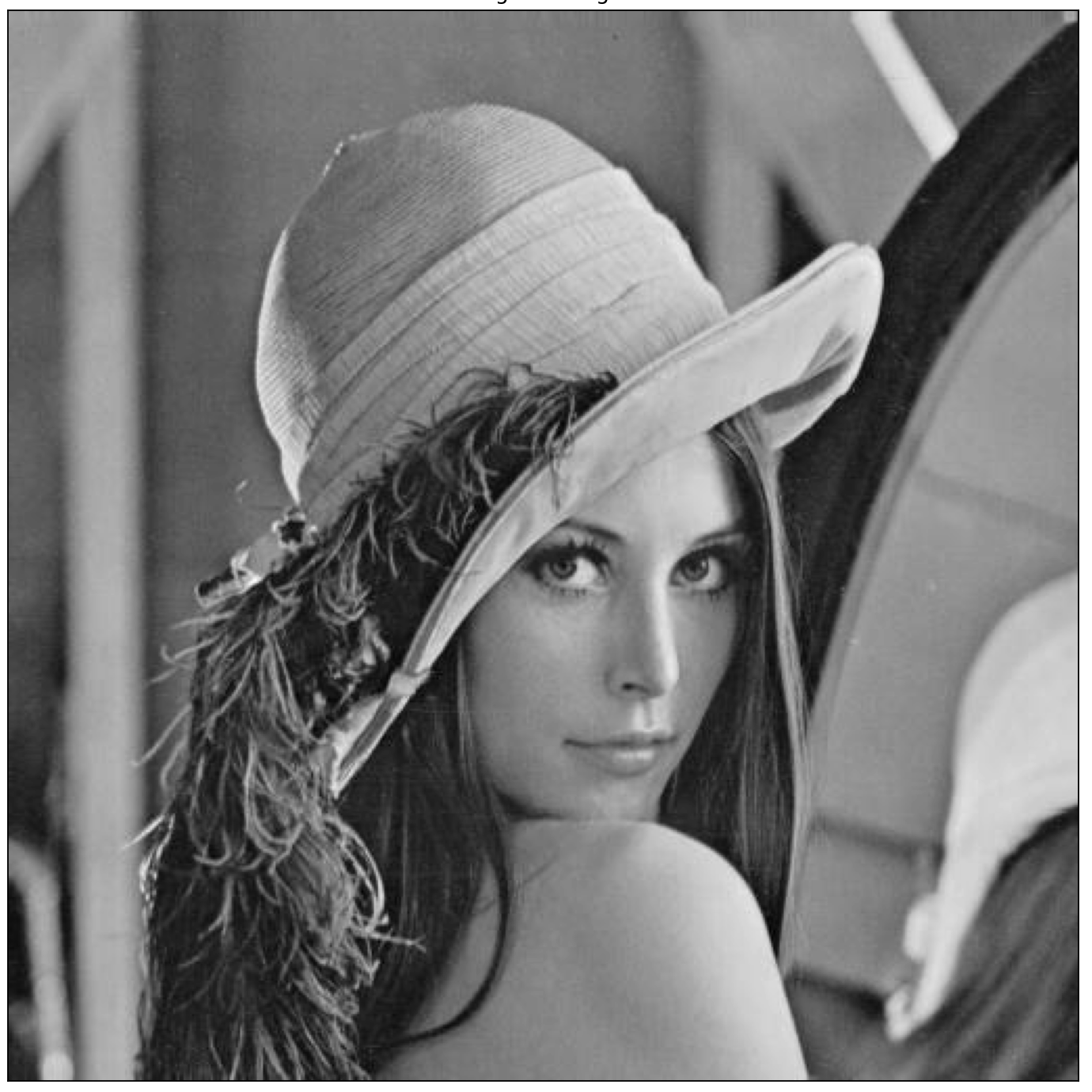
(a) Source Lena image.

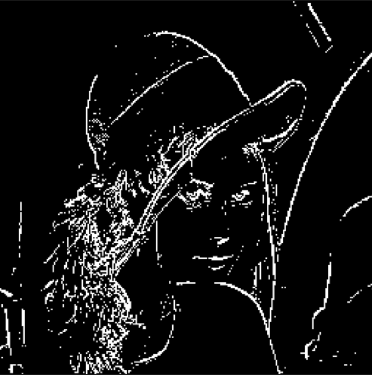
(b) Edge detection using Haar wavelet transform

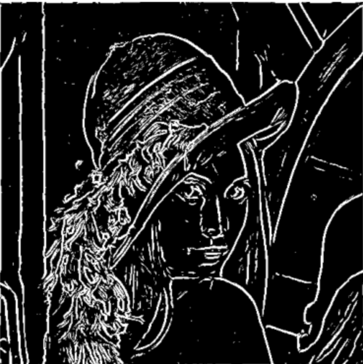
(c) Edge detection using CoShRem transform

Figure 1: wavelet transform fails to capture curvilinear edges which are successfully captured by the CoShRem.

These are the main reasons behind CoShNet’s novel architecture. CoShNet uses a complex Shearlet transform CoShRem [5] [6] and operates entirely in $\mathbb{C}$-domain. CoShRem does not have axis bias which wavelets suffers from, and handles edges of all orientations. Fig. 1 contrasts wavelets’ and shearlets’ ability to represent edges. CoShRem gracefully handles edges of varies orientations while wavelets struggles with some of them (curved or non-aligned to horizontal or vertical axes). CoShRem also gives us a critical property call “phase-congruency” [7], which keeps the features stable under perturbation and noise. Kovesi eloquently uses the agreement of phase across scale (frequency) to robustly localize an edge/ridge/blob while the gradients and magnitude can disagree extensively (fig 5). Phase-congruency will be covered in detail in S 3.2. This is in contrast to scattering and it’s use of complex-modulus which kills the critically important phase information. Recently, Wiatowski [8] shows us, CoShRem is a type of scattering and inherits its desirable property of deformation stability and can be efficiently implemented by FFT. Besides using a robust transform, CoShNet has the following desirable properties:

2 Contributions

• A Compact hybrid and efficient CNN architecture. CoShNet uses a fixed 2nd-generation wavelet transform to produce informative and stable representations for classification. In addition, through a series of tests, CoShNet has demonstrated state of the art results using a fraction of parameters ($49.9k$) versus ResNet-18 with $11.2m$. The architecture does not require any regularization nor hyperparameter tuning and is extremely stable with respect to initialization and training.

• Exceptional Generalization. Training with the $10k$ samples from Fashion and testing using the remaining $60k$ samples, we are able to obtain Top-1 accuracy close to $90\%$.

• Complex-valued neural network (CVnn) a CVnn has many attractive properties absent in its real valued counterpart. Nitta [9][10] studied the critical-points of real vs. complex neural networks and showed that a lot of critical-points of regular CNNs are local minima, whereas CVnn’s critical-points are mostly saddle-points. Nitta [11] also showed that the decision surface 4.1 of a CVnn has more representational power and is self regularizing. However, a good implementation in the complex domain is non-trivial. In S. 4 we will layout the important components for a efficient CVnn that performs competitively.

• Fully complex CVnn CoShRem is unique among CVnns as a fully complex network - all operations are performed using complex operators.

• Training a compressed model. We present a novel way of training a highly compressed version of CoShNet by using tensor compression and DCFNet [12] while preserving all of its good qualities. Unlike most efforts on model compression, the compressed model is trained in one pass.

Extensive experimental data presented here demonstrates that CoShNet trains much faster and uses less training data. All of the proposed models can be trained in less than $20$ epochs (some as low as $10$) in under 20 seconds on a modest GTX 1070Ti. Contrast that with a recent ResNet-50 based model which took 400 epochs to reach $91\%$ and has 28m parameters.

Finally, the structure of the paper is as follow: Section 3 discusses some critical properties of complex Shearlets and the importance of phase-congruency. Section 4 outlines the mathematics and implementation of complex-valued neural network (CVnn). Section 5 presents the simple architecture of CoShNet. Section 6 presents the highly compressed tiny-CoShNet. Section 7 presents the experimental results and ablation studies.

3 Hybrid CNN & Scattering

Raghu et al. showed in [13] that the lower levels of a CNN converge very early and that class-specific information is concentrated in the upper layers. Their proposal is to freeze the lower levels early. This confirms the central thesis of CoShNet for the role played by the lower levels in a classic CNN which is to learn an embedding. This article argues the embedding obtained by the CNN is largely generic - it has more to do with general “image statistics” and less to do with class-specific traits. Ravishankar et al. [14] “Deep Residual Transform” produce learned filters 2a which look very similar to those of K-SVD 2b, which is an exemplar of sparsity methods. These results inspired us to go one step further, and use a fixed signal transform instead of using a lot of capacity and time to learn a sparsifying transform. A fixed transform automatically implies better sampling efficiency and less affected by distribution or covariant shift.

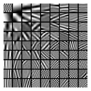
(a) Learned Transforms [14]

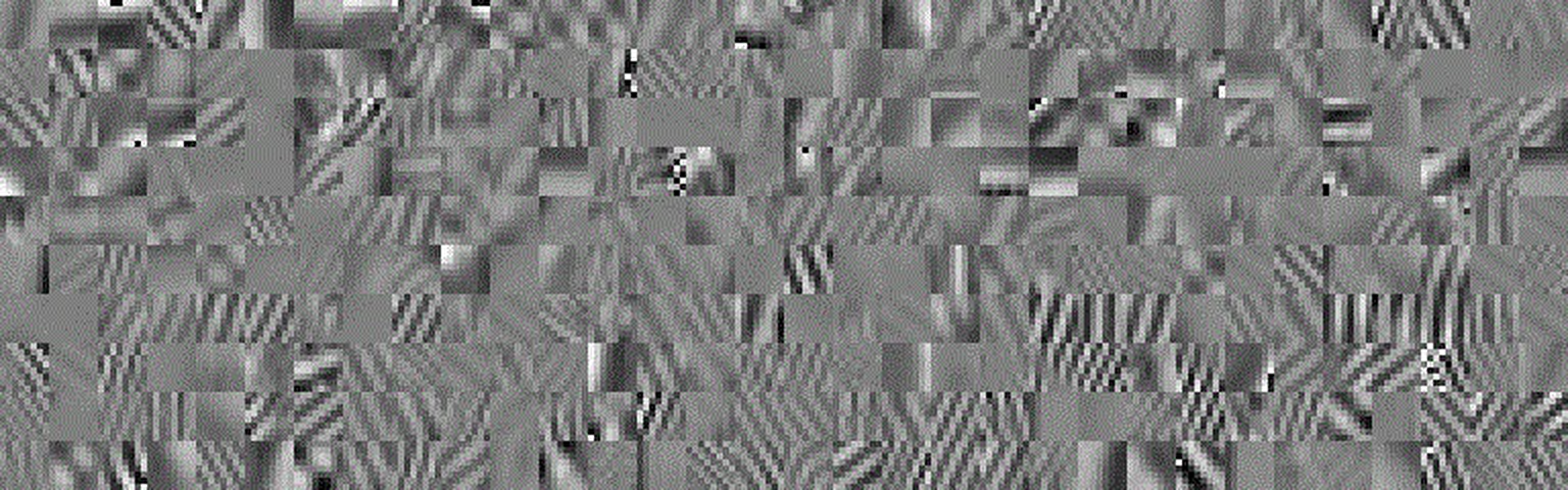
(b) Atoms from K-SVD for Sparse Encoding

Figure 2: a learned transform from [14] and atoms in a sparse encoding

Thus, CoShNet can be evaluated in the context of Oyallon & Mallat’s scattering-network [2]. Both are hybrid NN, and they replace the early layers in a CNN with a fixed transform that provide a sparse embedding for images. Mallat [3] also eloquently showed that scattering gave us the highly desirable property of local deformation stability and rotation invariance. However, scattering use complex-modulus after convolving with a Morlet wavelet 3 which kills the phase information. Phase encodes structure and is rich in semantics. CoShRem carefully preserves the phase across the cascade of scale and orientation by performing all operation in $\mathbb{C}$. We will discuss the critical role of phase in S 2.2.

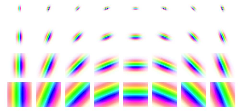
Figure 3: Real and imaginary parts of Morlet wavelets at 4 different scales and 8 orientations. Phase and amplitude are respectively given by the color and the contrast. Scattering and CoShRem both using filters that resemble Morlet wavelets.

3.1 CoShRem Transform

CoShRem is based on $\alpha$-molecules which is introduced in [15]. The transform is constructed by translating, scaling, and rotating members of a possibly infinite set of generator functions $\{\psi\}$. The scaling $a$ and shearing $s$ are applied to the arguments of the generator:

$$A_{a,\alpha}S_{s}\psi(x-t),$$ (1)

$$A_{a,\alpha}=\begin{bmatrix}a&0\\ 0&a^{\alpha}\end{bmatrix},\hskip 4.0ptS_{s}=\begin{bmatrix}1&s\\ 0&1\end{bmatrix},\hskip 4.0pta>0,\hskip 2.0pt\alpha\in[0,1],$$

$\alpha$ controls the anisotropy and smoothly interpolates the generator function to create a family of wavelets (isotropic scaling with $\alpha=1$), shearlets (parabolic scaling with $\alpha=0.5$) and ridgelets (fully anisotropic scaling with $\alpha=0$).

CoShRem can stably detects edges, ridges, and blobs [6] using phase and oriented filter-banks 5 without the need for unstable gradients. In Table 1, one can clearly see the filter’s alignment and the image features it detects. As a Fourier integral operator, CoShRem is stable and noise immune [16].

image / filter
	$11.13\%$	$1.03\%$	$1.04\%$	$10.17\%$
	$7.96\%$	$3.83\%$	$3.96\%$	$7.42\%$
	$4.43\%$	$7.35\%$	$7.73\%$	$4.16\%$
	$2.90\%$	$8.79\%$	$9.33\%$	$2.78\%$

Table 1: columns: 4 CoShRem filters, rows: MNIST. Each cell is the percentage energy of the filter response. In the first two rows, more energy is concentrated in the vertical aligned filters since both are dominated by vertical shapes and the opposite for remain two rows.

Reisenhofer at al. [6] show that the CoShRem transform is very stable in the presence of perturbations. Fig 4 shows despite the considerable perturbations (blurring and Gaussian noise), CoShRem remain stable to most of the characteristic edges and ridges (two step discontinuity in close proximity).

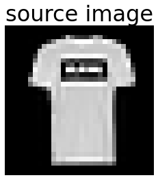
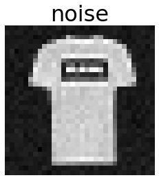
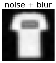
(a) image, noise($\sigma^{2}=50$), blur($\sigma=1$)

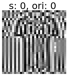
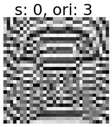
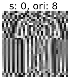
(b) phase without perturation

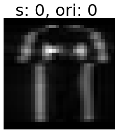
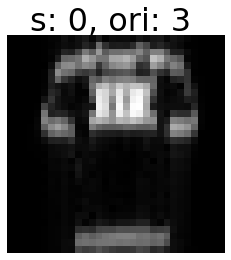
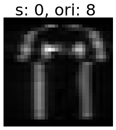
(c) magnitude without perturbation

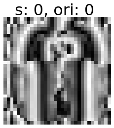
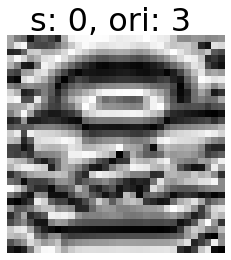
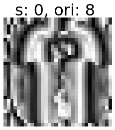
(d) phase with perturbation

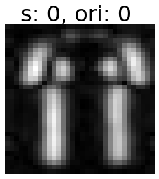
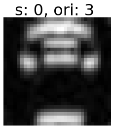
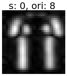
(e) magnitude with perturbation

Figure 4: (a) image and perturbations (b)..(e) CoShRem phase, magnitude

3.2 Phase & Phase-congruency

The important role of phase has been well established in signal processing. A motivating example is [17], [18] for encoding structure and semantics. Phase play a critical role in Kovesi [7]’s phase-congruency". He clearly show the power of agreement of phase across scales and orientation[19]. Reisenhofer et al. [6] and [20] show that with “phase-congruency", CoShRem can extract stable features - edges, ridges and blobs - that are contrast invariant. In Fig 6.b we can see a stable and robust (immune to noise and contrast variations) localization of critical features in an image by using agreement of phase. This is all the more striking in contrast to Fig 6 where gradients across scales wildly mismatch and are extremely sensitive to noise. In other words, gradients fluctuates wildly across scale but phase remains very stable at critical parts of the image.

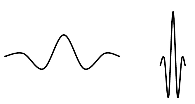
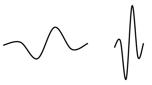
Figure 5: (a) even-symmetric Gabor (b) odd-symmetric Gabor

Phase congruency [21] in CoShRem is implemented using even-odd complex symmetric Gabor-pairs - filters of equal amplitude but orthogonal in phase - i.e. a $\pi/2$ offset (Fig. 5). See Phase congruency for more details. The pair is related by a Hilbert transform, which is the textbook method from Bracewell [22] to convert a real signal to a complex one. CoShNet thus inherits the desirable properties of the Hilbert transform.

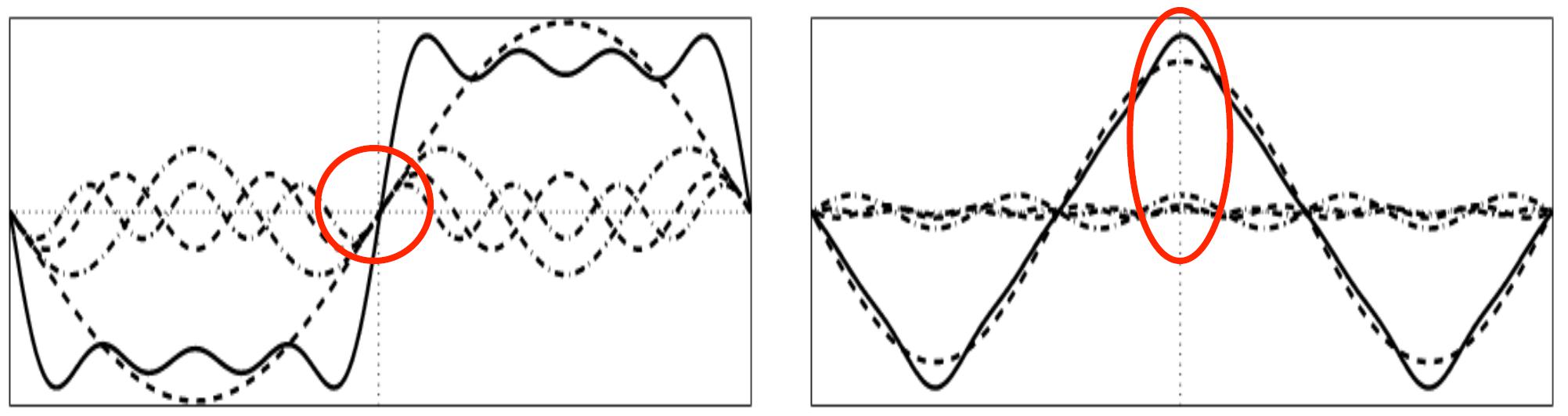
Figure 6: phase-congruency - (a) gradients across scales disagree (b) Fourier components are all in phase at the step in the square wave and at the peaks and troughs of the triangular wave. Images generated using [23].

4 Complex-Valued Neural Networks (CVnns)

Given the importance of phase and CoShRem being a complex transform, it seems natural for the network to be complex-valued. A CVnn has complex inputs, weights, biases and activations with all the mathematical operation performed in $\mathbb{C}$. It requires a complex version of backprop [24] demanding careful analysis and efficient implementation 4.4. It can be traced back to the pioneering work of Nitta [25] and Hirose [26]. It has several attractive properties such as orthogonal decision boundaries and attractive structure among its critical points, which are particularly powerful, but not well known.

4.1 Complex Decision Boundary, Critical Points & Generalization

Nitta’s [9], [11] seminal work shows the CVnn has the following remarkable properties not found in standard CNNs -

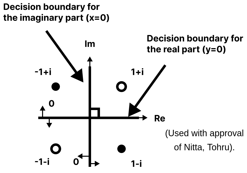
Figure 7: Decision boundary formed by a neuron of a CVnn.

1. Orthogonality of decision boundaries: The decision boundary of a CVnn consists of two hypersurfaces that intersect orthogonally (Fig. 7) and divides a decision region into four equal sections. Furthermore, the decision boundary of a 3-layer CVnn stays almost orthogonal [27]. This orthogonality improves generalization. As an example, several problems (e.g. Xor) that cannot be solved with a single real neuron, can be solved with a single complex-valued neuron using the orthogonal property.

2. Structure of critical points: Nitta shows most of the critical points of a CVnn are saddle points, not local minima [10], unlike the real-valued case [28]. The derivative of the loss function is equal to zero at a critical point. SGD with random inits can largely avoid saddle points [29] [30], but not a local minimum.

3. Generalization: a CVnn trains several times faster than regular CNN and generalizes much better. Nitta [27] show they are both connected to Orthogonality property. We will show in our experimental section how our CVnn can be trained with $1k$ data and 20 epochs with excellent results.

Our finding is in strong agreement of with all three of Nitta’s findings. The power of a NN is determined by its ability to model complex decision boundaries [31]. A CVnn is endowed with a much more powerful ability to represent complex decision surfaces due to Orthogonality property 1.

4.2 Complex Product & $2\times 2$ Orthogonal Matrix

In neural networks, most of the heavy lifting are performed by linear-operators $z=W\times x+b$. For the $\mathbb{C}$ valued case, the complex-linear (ear) operator becomes:

$$z=\mathbb{R}(W)\times\mathbb{R}(x)-\mathbb{I}(W)\times\mathbb{I}(x)+i(\mathbb{I}(W)\times\mathbb{R}(x)+\mathbb{R}(W)\times\mathbb{I}(x))+b$$ (2)

In terms of operator count, a cplx-linear is 4 times more expensive than a real one. We will later show the actual performance difference is considerably less with a good implementation. The cplx-linear used in CoShNet follows Hirose [32] and treats complex as a $2\times 2$ orthogonal matrix. Given $\mathbb{C}$-linear transform $T_{c}:c=a+ib$:

$$T_{c}\begin{pmatrix}x\\ y\end{pmatrix}=\begin{pmatrix}ax-by\\ bx+ay\end{pmatrix}=\begin{pmatrix}a&-b\\ b&a\end{pmatrix}\begin{pmatrix}x\\ y\end{pmatrix}$$ (3)

The linear transform $c=a+ib$ is represented by the matrix $\begin{pmatrix}a&-b\\ b&a\end{pmatrix}=r\begin{pmatrix}cos\theta&-sin\theta\\ sin\theta&cos\theta\end{pmatrix}$. This is easily recognizable as a planar rotation matrix and is directly used in the “split-layer” 4.3 of CoShNet. Alternatively one may also write complex multiplication (cplx-mult) as amplitude-phase - i.e. $z_{1}=a_{1}e^{i\theta_{1}}$ and $z_{2}=a_{2}e^{i\theta_{2}}$:

$$a_{1}e^{i\theta_{1}}a_{2}e^{i\theta_{2}}=a_{1}a_{2}e^{i(\theta_{1}+\theta_{2})}$$ (4)

Thus, cplx-mult is equivalent to amplitude scaling and phase addition or shift. The significance of phase cannot be overstated, since phase encodes shifts in time for wave signals or position in images. The polar form is valuable for physical intuition, but its direct use in CVnn is less attractive as Nitta [33] shows a polar CVnn is unidentifiable.

4.3 Efficient complex-linear operator

The proposed CVnn is implemented using “split-layers” i.e. to store and propagate real and imaginary parts as two independent real tensors [34]. This enables it to leverage existing and highly optimized code of PyTorch (e.g. real-Autograd) and other repos since most are in $\mathbb{R}$ domain. Split-layer use a SoA (Structure-of-Arrays) layout and is critical for efficient SIMD/GPU code.

Since real and imaginary components are propagated separately, one might be tempted to ask if a CVnn is just a $2\times$ RVnn. Hirose’s works [26], [35] encourage us to look at cplx-mult as a $2\times 2$ orthogonal matrix or operating in amplitude-phase space as shown in section 4.2. The real and imaginary components might be stored separately, but they are far from just $2$ real channels. The cross-terms in eq 2 are critical for this intuition (See [36] for more details). The cross-terms allow information to flow between the real and imaginary part. This is also the approach taken by SurReal [37] which model complex as a product manifold of scaling and planar rotations. Complex scaling naturally becomes a group of transitive actions.

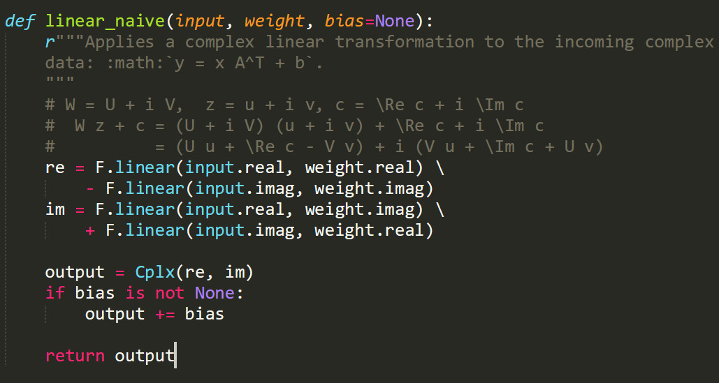
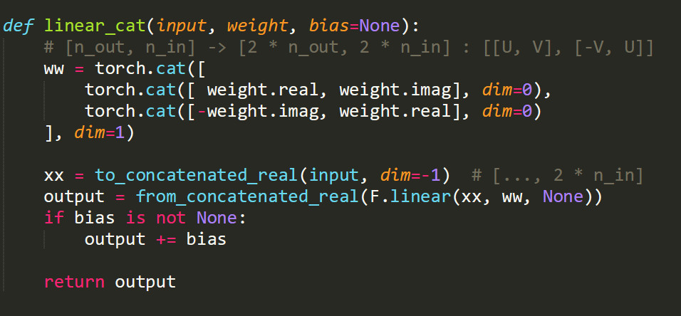
Figure 8: cplx-module L: naive cplx-linear R: eq 3 in code

CoShNet’s cplx-linear layers directly use eq.3 for cplx-mult . This enables the highly optimized autograd of PyTorch to seamlessly provide gradient support without special coding and saves GPU time.

4.4 Efficient Differentiation/Backprop in Complex Domain

The field of complex values is unordered; hence a CVnn is modeled as $f:\mathbb{C}\rightarrow\mathbb{R}$ with a real loss function $\mathcal{L}$. Cauchy-Riemann equation requires a complex differentiable function to be holomorphic. However, ReLU is non-holomorphic because it is unbounded. Let’s examine how Wirtinger calculus [38] circumvents the holomorphism requirement.

Similar to the $4\times$ problem of forward pass, during regular backprop a gradient is just $\dfrac{\partial L(z)}{\partial(z)}$. For cplx-backprop the direction of steepest ascent is given by its conjugate-gradient 5 which required 4 partials:

$$\dfrac{\partial L}{\partial z^{*}}=\dfrac{\partial L}{\partial u}\times\dfrac{\partial u}{\partial z^{*}}+\dfrac{\partial L}{\partial v}\times\dfrac{\partial v}{\partial z^{*}}$$ (5)

Let us have a look at Wirtinger’s complex differentiation. Let $f$ be a function of reals $a$ and $b$. We can write $f(z,z^{*})=f(a,b)$ where $z=a+ib$ and its complex conjugate $z^{*}=a-ib$. Wirtinger’s derivatives are:

$$\frac{\partial f}{\partial\mathbf{z}} = \frac{1}{2}\left(\frac{\partial f}{\partial a}-i\frac{\partial f}{\partial b}\right),$$ (6)

$$\frac{\partial f}{\partial\mathbf{z^{*}}} = \frac{1}{2}\left(\frac{\partial f}{\partial a}+i\frac{\partial f}{\partial b}\right).$$ (7)

Eq. 6 gives CVnns the ability to use non-holomorphic activation functions, which are often shown to outperform holomorphic ones. Trabelsi [34] explored several complex activations and found the simplest split-ReLU to be the best. ELU was explored in [39] because of its negative half-space response (which has interesting properties). We found it to be closely behind split-ReLU in experiments. Both equations in 6 are necessary-and-sufficient, only conjugate-gradient ($\frac{\partial f}{\partial\mathbf{z^{*}}}$) is needed using two partials:

$$\dfrac{ds}{dz^{*}}=\dfrac{dL}{ds^{*}}\times(\dfrac{ds}{dz})^{*}$$ (8)

The gradient sharing trick is used by PyTorch. In contrast, cplx-linear directly use the matrix interpretation in our 4.3. See 8 in supplement. The difference of making this choices can be seen in the performance difference between CoShNet using cplxmodule (which uses the $2\times 2$ multiplication during forward) vs. native complex type of PyTorch (which does not use $2\times 2$ multiplication). Porting entire CoShNet to PyTorch 1.9 native complex tensors, it takes 0.192 and 0.355 seconds for forward and backprop respectively. By comparison the cplxmodule based model takes 0.099 and 0.184 - i.e. twice as fast. This difference is also partially attributed to SoA in our ’split-layer’ vs. AoS (Array-of-Structures) used by PyTorch.

4.5 Complex initialization

Good initialization is critical to a CNN. Trabelsi et al. [34] followed Xavier’s [40] reasoning to derive the initialization for complex weights. Key insight is a complex Gaussian modulus follows a Rayleigh distribution $\frac{x}{\sigma^{2}}e^{-x^{2}/2\sigma^{2}}$. For weights $W$:

$$Var(W)=Var(|W|)(\mathbb{E}(|W|)^{2})$$ (9)

We now have a formulation for the variance of $W$ in terms of the variance and expectation of its magnitude, both are analytically computable from the Rayleigh distribution’s single parameter $\sigma$, indicating the mode. These are:

$$\mathbb{E}(|W|)=\sigma\sqrt{\frac{\pi}{2}},\quad Var(|W|)=\frac{4-\pi}{2}\sigma^{2}$$ (10)

Xavier provides a good scaling to keep the outputs and gradients to be the same order of magnitude. We set $\sigma=\sqrt{\frac{Var[W]}{2}}=1/\sqrt{n_{in}+n_{out}}$. The magnitude of the complex parameter $W$ is then initialized using the Rayleigh distribution with $\sigma$. The phase is uniformly initialized in range $[-\pi,\pi]$ to make sure phase is covered evenly.

5 CoShNet Model

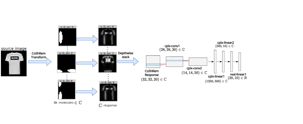
Figure 9: CoShNet with 2 cplx-conv and 3 cplx-linear layers. Images are transformed by CoShRem in the data pipeline but acts as a fixed input layer. Its only uniqueness being its use of complex operators.

Fig 9 shows the architecture for CoShNet. Each of the two convolutional layers has $2\times 2$ average-pooling and split-ReLU activation. Following this, the response map is flattened and propagated through $2$ cplx-linear layers. Next, the real and imaginary components of response are concatenated and passed through an additional linear layer which feed the cross-entropy loss. CoShNet operates entirely in $\mathbb{C}$ until the last layer. Especially in the fully connected linear layers to take advantage of the orthogonal decision boundary of complex layers. CoShNet is initialized with cplx-init from Trabelsi et al. discussed in 4.5.

The proposed CVnn is notable for what it does not have:

1. data-augmentation is often used to learn a stable embedding. CoShNet is endowed with a embedding stable to perturbations due to CoShRem’s properties.

2. skip-connections is usually needed for deep models to pass the higher resolution signals to upper layers. CoShNet uses a multi-scale transform and naturally preserve signal resolution.

3. batch normalization is needed in deep models to combat vanishing gradients. CoShNet only needs 5 layers to achieve good performance and do not suffer from vanishing gradients.

4. weight-decay and dropout regularization are not needed.

5. learning rate schedule and early stop are usually used to avoid overfitting. CoShNet avoided overfitting with a fixed transform. In the experiment section one can see CoShNet is very stable to training regime and initialization 6.

6. hyper-parameter tuning is important for RVnns and considerable effect usually goes into it. CoShNet is very stable towards change in learning rate, number of epochs, batch size etc. as shown later in section 7.

CoShNet uses Adam’s defaults with a fixed learning rate of $0.001$ and trains on very modest number of epochs (maximum $20$). It use batch-size of $128$ when training on the 10k set and $256$ when training on 60k.

This is in stark contrast to a recent paper [41] “.. the necessity to optimize jointly the architecture and the training procedure: ..having the same training procedure is not sufficient for comparing the merits of different architectures.” Which is the opposite of what one wants to have - a no-fuss, reliable training procedure for different datasets and models.

5.1 Strengths of CoShNet

Previous efforts to develop CVnns [34], [42], [37] mostly were split-CVnns and ignored the special properties of $\mathbb{C}$ (4.2, 4.3) or switch from $\mathbb{C}$ to $\mathbb{R}$ in the middle [43]. Others did not use special initialization 4.5 required for complex weights. Still earlier CVnns spend large effort on finding good complex holomorphic activation which were found to be inferior to split-ReLU. Others have inefficient back-prop, while Trabelsi et al. [34] require BatchNorm and learn-rate search.

CoShNet is probably the most thorough CVnn, it stays in $\mathbb{C}$ domain especially in the MLP layers 9. Naturally this is inspired by Nitta’s decision boundary and critical point 4.1 analysis. CoShNet is a fully complex CVnn while the better known work by Trabelsi et al. [34] and SurReal [37] are really partial complex/real-CNNs. While SurReal treated the merits of a fully complex NN most thoroughly, it still switch to real after their DIST layer. The MLP layers within a CNN performs the actual classification, which means it is critical for it be endowed with the orthogonal property discussed in S 4.1. CoShNet use two cplx-linear layers to form its MLP block.

Another strength of CoShNet in the context of CVnns is how it maps real-valued images into $\mathbb{C}$ domain. In well known CVnns, the imaginary component is set to $0$ while Trabelsi et al. [34] uses a single residual block to learn the imaginary component. Phase recovery is notoriously difficult. CoShNet use complex even-odd symmetric Gabor-pairs and the Hilbert transform as covered in S. 5. CoShNet uses this principled method from classic signal processing [22]. Instead of treating it as a real to complex conversion, CoShNet uses a spatial to frequency transform (CoShRem) which encodes the semantic structure of the image in phase.

5.2 Prior works in CVNN

CoShNet leveraged these building blocks [34], [42], [37] for CVNN especially the excellent cplxmodule by Nazarov. We integrated and adapted all of them into a coherent and efficient framework shnetutil and are releasing it as a building block for other researchers.

https://github.com/Ujjawal-K-Panchal/coshnet

6 Compressing CoShNet with DCF, Tensor-Train & tiny

Although the CoShNet is quite efficient with respect to generalization and training times. Its 1.3m parameters when compared to a ResNet18 (11.18m parameters) is very good. There is room for improvement. In a CNN the bulk of the computation resides in the convolutional layers while most of the parameters are in the linear layers. CoShNet attacks it on these two fronts - adopting DCFNet [12] to optimize the cplx-conv layers and Tensor-Train [44] for the cplx-linear layers. The result is a highly compressed tiny-CoShNet. It only has $49.9k$ parameters, which is $1/221$ that of ResNet-18, and still achieves SOTA performance on Fashion MNIST.

6.1 Decomposed Convolutional Filters

DCFNet [12] decomposes convolutional filters into a truncated expansion using a fixed Fourier-Bessel dictionary in the spatial domain (Fig.10). Only the expansion coefficients are learned from data. Representing the filters in functional bases reduce the number of trainable parameters to those of the expansion coefficients ($KM^{\prime}\times M$) where $K$ is the number of basis we select from the dictionary. DCFNet can be seen as dictionary-learning applied to a convolution kernel. In addition, the Fourier-Bessel bases captures the low-frequency component which helps to counteract the tendency for CNN to over emphasize fine details, thus reducing overfitting . Thus, DCFNet approximate the Toeplitz-matrix $W_{\lambda^{\prime},\lambda}(u)$ of the convolution kernel by $W_{\lambda^{\prime},\lambda}(u)=\sum\limits_{k=1}^{K}(a_{\lambda^{\prime},\lambda})_{k}\Psi_{k}(u)$ using $K$ atoms $\Psi_{k}$:

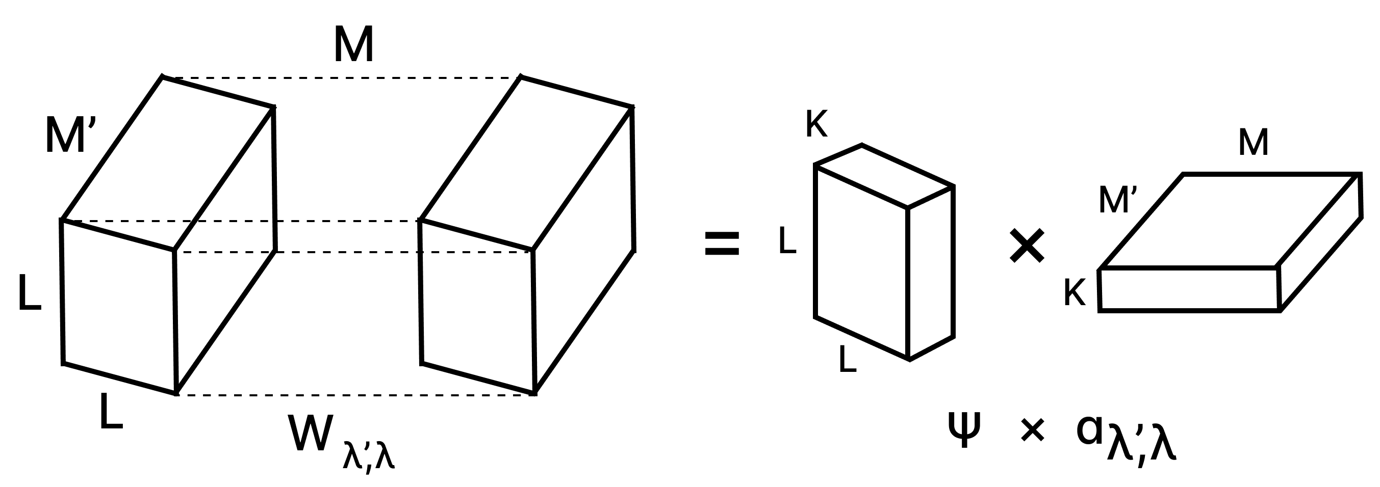
Figure 10: DCFNet: $L\times L\times M^{\prime}\times M$ conv-layer is decomposed into $K$ atoms of size $L\times L(\Psi)$ and $KM^{\prime}\times M$ coefficients $a$ where $\Psi$ is fixed and $a$ is learned.

$K=3$ was found to be sufficient for high accuracy. Hence the savings is $\frac{K}{L^{2}}\approx\frac{1}{8.3}$ for $L=5$ (for $5\times 5$ convolution used in CoShNet).

6.2 Tensor Decomposition & $49.9k$ tiny-CoShNet

Over $90\%$ of the parameters in CoShNet are in the linear layers. We apply Tensor-Train factoring to compress them. Oseledets [44] introduce the Tensor-Train (TT) factorization to approximate the $W\in\mathbb{R}^{M\times N}$ in a linear layer: $f(x)=W\cdot x+B$ using a product factorization:

$$\mathcal{A}(j_{1},j_{2},\ldots,j_{d})=\mathbf{G}_{1}[(j_{1})]\mathbf{G}_{2}[(j_{2})]\ldots\mathbf{G}_{d}[(j_{d})]\approx W$$ (11)

Tensor-Train (TT) in CoShNet can be seen as a complex version of TT-layer of Novikov et al. [45] which introduced TT to deep learning.

The number of terms in the factorization $\{r_{k}\}^{d}_{k=0}$ is the TT-ranks which controls the approximation quality. The collections of matrices $\mathbf{G}_{k}$ are called TT-cores - each is a $3D$ tensor. All matrices related to the same dim $k$ are restricted to be of size $r_{k-1}\times r_{k}$. The rank on the first and last core must be $R_{1}=R_{N+1}=1$ to ensure scalar input and outputs. . The approximation error is controlled by the maximum rank $r_{max}$. Storage of TT decomposition depends linearly on the number of dimensions unlike e.g. Tucker which is exponential. It also has robust approximations algorithms (tt-svd [44]) which we leveraged to produce tt-svd-init 6.2.1 covered in the next section. TT also efficiently supports basic linear algebra operations.

In tiny-CoShNet the above two compressions are applied - DCF for the two cplx-conv and TT-layer [45] for the largest of its fully-connected layer. The stunning fact is how small tiny-CoShNet is - $49.9k$ (from $1.3m$). Converting the dense $1250\mathsf{x}500$ FC-layers to a rank-$8$ TT format ($50\mathsf{x}1\mathsf{x}8\mathsf{x}20$) reduced the parameters by $45\times$ (from $1.25m\mapsto 2.7k$) without sacrificing the expressive power of the layer. Unlike earlier works which first train an uncompressed model and then apply TT to compress. The tiny-CoShNet is constructed with TT-layer before training. This saves considerable time since one does need neither to iterate to compress nor re-train after compression.

6.2.1 tt-svd-init

Tensor-Train conceptually seems straight forward, but to implement it well in a CVnn is not so obvious. First, TT-layer [45] is implemented with cplx-linear. For initialization, at first CoShNet follow other ML researchers and use a simple random or Xavier init for each tensor-core and the results are not competitive. Instead tiny-CoShNet first initialize a dense nn.linear with cplx-init from Trabelsi et al. [34]. Next, tt-svd [44] is used to find the best rank-$k$ TT approximation for the initialized dense layer. This ensures the TT-layer behaves like a Xavier initialized cplx-linear layer at the start of training. This might seems obvious, but the authors are not aware of previous publications that approached it this way. Good initialization was found to be key and is a novel contribution of tiny-CoShNet. This enable tiny-CoShNet to use an aggressive compression factor of $45\times$ without sacrificing performance.

Supplement details ablation studies where each of the two methods were applied separately.

7 Experiments & Ablations

To test the hypothesis that CoShNet needs less training data and generalizes better most training is performed using the 10k test set of Fashion-MNIST [46] and 60k train set to test. Additional results using $1k..5k$ to train are in table 7 .

MNIST is known to be too simple as a dataset, but it is still ubiquitous. To make it harder we use the 10k test set to train and $60k$ for test, the top-1 accuracy after 20 epochs is $98.2$. Additional MNIST results are in Table 2. All of the remaining experiments use Fashion-MNIST.

Table 2 compares the performance of the already small base-CoShNet ($1.3m$) and the even smaller tiny-CoShNet ($49.9k$). In the last column of the table, the full training set (60k) is used to make it easier to compare against other published results. If we place its performance against the FashionMNIST leaderboard, both $92.2$ and $91.4$ place us $8^{th}$ position in the research papers leaderboard. The $7^{th}$ place use a VGG model with $528m$ parameters. A Resnet-18 based model with $11.18m$ parameters achieved $91.8$ vs. $92.2$ for base-CoShNet.

Model	Dataset	size	epochs	10k training	60k training
base	Fashion	$1.36m$	$20$	$89.2$ (20 epoch)	$92.2$ (20 epoch)
tiny	Fashion	$49.9k$	$20$	$88.2$ (18 epoch)	$91.4$ (20 epoch)
base	MNIST	$1.36m$	$20$	$98.2$ (20 epoch)	$99.1$ (10 epoch)
tiny	MNIST	$49.9k$	$20$	$98.1$ (16 epoch)	$99.2$ (20 epoch)

Table 2: base-CoShNet vs. tiny-CoShNet on Fashion & MNIST

tiny-CoShNet Top-1 accuracy is already within $1.0\%$ (88.2 vs 89.2) of the base-model. Next a simple "learning rate schedule" is performed to see what if any difference it might make.

7.0.1 tiny-CoShNet with learning-rate schedule and over training

A simple trial was done with: 5 epochs at lr=0.01 & 15 at lr=0.002. The schedule is partially inspired by Tishby’s 2018 Stanford lecture in which he described the "two-phases of NN training dynamics" [47]. From table 3 one can see the tiny $49.9k$ model is neck-to-neck with the baseline using the schedule. The best model was trained in 10 epochs! The 80 epoch test also shows both models do not degrade with over-training.

Model	size	20 epochs: 60K best	80 epochs: 60K best
base	$1366390$	89.2(20E)	89.9(77E)
tiny + lr_schedule	$49990$	$89.1$(10E)	$89.0$ (10E)

Table 3: 10K20E|10K80E, base-model vs. tiny+lr_schedule, train=$10k$, test=$60k$, size = number of parameters

7.1 CoShNet vs. ResNet-18/50

This section is dedicated to comparison of CoShNet against the popular ResNet-18 and ResNet-50 in terms of model size, training efficiency, performance, FLOPs etc.

7.1.1 Model Size & Convergence

As shown in following table 4, despite it smaller size (1/8.6), CoShNet-base is consistently better than ResNet-18 in final performance and convergence speed (20 vs. 100 epochs). The tiny-CoShNet is even more impressive as it is $1/(11.18*1024/49.99)\approx 1/229$ the size of ResNet-18 but is neck-to-neck with it.

Model	Epochs	# of Parameters	Size Ratio	Top1 Accuracy (60k)	Accuracy (10k)
ResNet-18	100	11.18M	229	91.8%	88.3%
ResNet-50	100	23.53M	481	90.7%	87.8%
CoShNet (base)	20	1.37M	28	92.2%	89.2%
tiny-CoShNet	20	49.99K	1	91.6%	88.0%

Table 4: CoShNet vs. ResNet for Fashion. CoShNet was only trained for 20 epochs versus 100 for ResNet.

Here, 60k means training on the training set (60k) and testing using the 10k test set. Similarly, 10k means training on the test set and testing on training set.

7.1.2 FLOPs comparison

In table 5, we compare the number of FLOPs per batch for CoShNet and ResNet.

Model	Batch Size	FLOPs	FLOP Ratio
ResNet-18	128	4.77 GFLOPs	52.48
ResNet-50	128	10.82 GFLOPs	119
CoShNet (base)	128	93.06 MFLOPs	1

Table 5: FLOPs for CoShNet and ResNet.

CoShNet consume $93$ MFLOPs while ResNet-18 need $4.77$ GFLOPs which is $52$ times more. ResNet-50 use $119$ times more FLOPs. CVNN usually is considered to be $4\times$ more expensive than their real valued networks. We can see this is not the case for CoShNet.

7.2 Initialization, Batchsize and learning-rate stability tests

Picard [48], while studying the influence of random seeds concluded: “it is surprisingly easy to find an outlier that performs much better or much worse than the average”. On the contrary, Table 6 shows the impact of random seeds is negligible for CoShNet. The number of epochs needed to reach the ‘best model’ also is very stable. While $4k$ seeds were not tested, the entire model is trained from scratch each time with a different seed and not just 1 layer like [48].

random seed	89.5	89.4	89.3	89.4	89.1	89.6	89.5	89.1	89.7	89.4	89.3
batchsize 32..1024	89.2	89.4	89.5(128)	89.4	89.8	89.5	89.4	89.6	89.3	88.5	87.2(1024)
lr (.001..01)	89.3	88.8	88.8	89.0	88.9	88.7	88.7	88.3	88.3	88.5

Table 6: Top-1 accuracy for different random seeds/batch sizes/learning-rate, train $10k$ test $60k$, 20 epochs

Similar to initialization, batch sizes ($32|64|128|160|192|224|256|288|320|512|1024$) and learning rates are evaluated in second and third row of 6. Again the results are very stable. For scientific integrity, only default initialization and batch size is quoted in all the results in this paper. One can see some small potential gain if one is willing to do hyperparameter tuning - e.g. batch size of 192 is $.3\%$ higher. Even then the gain is not dramatic. Astute reader will notice CoShNet trained with 10k data and batch of 1024 still performs remarkably well (87.2).

7.2.1 CoShNet generalization, data efficiency & RVNN

Recent results by Barrachina et al. [49] also confirm our finding that CVnn do not need drop-out and still generalizes well. Unlike for RVNN where the authors reported a drop from $92\%$ to $66\%$ without drop-out.

Additionally, Table 7 show using as little as $1k$ to $5k$ training data from Fashion while testing using $60k$, CoShNet managed an accuracy of around $82..87\%$. With 100 samples per class, this is almost in the Few-Shot regime. In addition, the variability among different subsets of the same size also is small.

training set	1k	2k	3k	5k	10k
best model	${82.2|81.7|81.8}$	${84.7|85.0|84.6}$	${85.9|85.3|85.8}$	${87.0}|{87.0}|{87.7}$	${89.1}$

Table 7: CoShNet when trained on differently sized subsets of the test set and tested on the 60k training set. The variability among different subsets of the same size is also small in each cell.

7.3 CoShNet under Perturbation & Noise

As described previously in section 3, CoShRem Shearlet transform demonstrate good robustness to perturbations such as noise and blur. In this section we investigated if this visual robustness translates to better inference and generalization within the CoShNet. The dataset is perturbed with random Gaussian noise ($\mu=0,\sigma^{2}=10.0$) and random Gaussian blur filter ($\sigma\leq 0.75$). CoShNet is trained with different combinations of clean (c) (no perturbation nor noise) and/or perturbed (p) test and/or train sets. The best performance is shown in the following figure 11.

Decent performance in the face of perturbation suggests that the CoShNet is fairly robust to presence of perturbation.

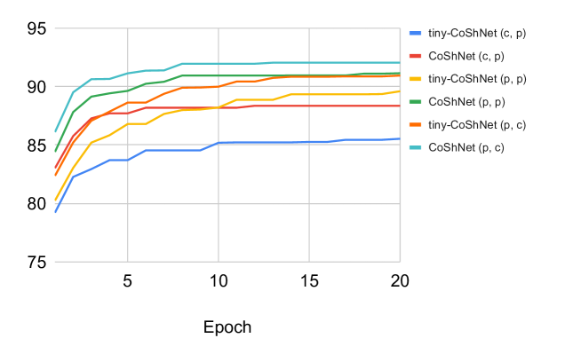
Figure 11: Robustness in presence of perturbation and noise. In legend, clean is abbreviated as ’c’, perturbed is abbreviated as ’p’. CoShNet(c, p) means it is trained on a clean training set and then tested on a perturbed test set. Likewise, all other combinations for CoShNet and tiny-CoShNet are trained for 20 epochs and best test-accuracy is reported.

8 Conclusion

This article introduced a novel hybrid-CVnn architecture using complex-valued shearlet transform. It is more than $200\times$ smaller than ResNet-18, use $100\times$ less FLOPs and train faster than their real valued counterparts for similar performance. It generalizes extremely well and trains with little labeled data. CoShNet trains fast without hyperparameter tuning, learning rate schedules, early-stops, batchnorm or regularization etc.

CVnn have been found to give superior results in naturally complex signals (e.g. MRI [50], SAR [50], RF [51] etc. ), but a recent study [52] found CVnn to not be competitive for images or have difficulties with training [53]. Experimental results herein challenge us to reassess. A principled conversion of real to complex is critical as well as thoroughly treating all the building blocks of a fully complex-CNN.

Compelling results using DCF and Tensor-Train in a compressed CVnn (tiny-CoShNet) and directly training the compressed model should be of independent interest.

Besides mobile and IoT applications where model size and real-time response is valued, the tiny-CoShNet can be an effective block in other architectures. Such as routing-transformer, twins, network-in-network, which requires instantiating many NN within a larger network.

9 Acknowledgements

We would like to thank Ivan Nazarov, Ivan Barrientos, Rey Medina, Enrico Mattei, Tohru Nitta, Rudrasis Chakraborty for their valuable advice.

References

- [1] M. C. Jonathan Frankle, “The Lottery Ticket hypothesis: Finding Sparse, Trainable Neural Networks,” in ICLR ’19, vol. 2, p. 42, 2019.
- [2] E. Oyallon and S. Mallat, “Deep roto-translation scattering for object classification,” in CVPR, vol. 07-12-June, pp. 2865–2873, IEEE Computer Society, oct 2015.
- [3] J. Bruna and S. Mallat, “Invariant Scattering Convolution Networks,” PAMI, vol. 35, pp. 1872–1886, Aug 2013.
- [4] C. Szegedy, W. Zaremba, I. Sutskever, J. Bruna, D. Erhan, I. Goodfellow, and R. Fergus, “Intriguing properties of neural networks,” in ICLR ’14, 2014.
- [5] G. Kutyniok, W. Q. Lim, and R. Reisenhofer, “ShearLab 3D: Faithful Digital Shearlet Transforms based on Compactly Supported Shearlets,” ACM Trans on Mathematical Software, vol. V, no. 212, pp. 1–39, 2014.
- [6] R. Reisenhofer and E. J. King, “Edge, Ridge, and Blob Detection with Symmetric Molecules,” SIAM J on Imaging Sciences, vol. 12, no. 4, pp. 1585–1626, 2019.
- [7] P. Kovesi, “Image Features from Phase Congruency,” J of Comp. Vision Res., vol. 1, p. 27, 1999.
- [8] T. Wiatowski and H. Bölcskei, “Deep Convolutional Neural Networks Based on Semi-Discrete Frames,” in IEEE Int Symp on Information Theory, pp. 1212–1216, 2015.
- [9] T. Nitta, “On the critical points of the complex-valued neural network,” in ICONIP, vol. 3, pp. 1099–1103, 2002.
- [10] T. Nitta, “Local minima in hierarchical structures of complex-valued neural networks,” Neural Networks, vol. 43, pp. 1–7, 2013.
- [11] T. Nitta, “Orthogonality of Decision Boundary in Complex-valued Neural Networks,” Neural computation ’03, vol. 16, no. 1, pp. 73–97, 2003.
- [12] Q. Qiu, X. Cheng, R. Calderbank, and G. Sapiro, “DCFNet: Deep Neural Network with Decomposed Convolutional Filters,” in ICML, vol. 9, pp. 6687–6696, feb 2018.
- [13] M. Raghu, J. Gilmer, J. Yosinski, and J. Sohl-Dickstein, “Svcca: Singular vector canonical correlation analysis for deep learning dynamics and interpretability,” 2017.
- [14] S. Ravishankar and B. Wohlberg, “Learning Multi-Layer Transform Models,” arXiv:1810.08323, p. 6, oct 2018.
- [15] P. Grohs, S. Keiper, G. Kutyniok, and M. Schäfer, “-molecules: curvelets, shearlets, ridgelets, and beyond,” in Wavelets and Sparsity XV, vol. 8858, p. 34, 2013.
- [16] K. Guo and D. Labate, “Representation of Fourier Integral Operators Using Shearlets,” J of Fourier Analysis and Applications ’08, vol. 14, no. 3, pp. 327–371, 2008.
- [17] T. S. Huang, J. W. Burnett, and A. G. Deczky, “The Importance of Phase in Image Processing Filters,” ASSP ’75, vol. 23, no. 6, pp. 529–542, 1975.
- [18] A. V. Oppenheim and J. S. Lim, “The Importance of Phase in Signals,” Proc of the IEEE ’81, vol. 69, no. 5, pp. 529–541, 1981.
- [19] P. Kovesi, “Phase Congruency Detects Corners and Edges,” in Digital Image Computing Techniques and Applications ’03, p. 10, 2003.
- [20] H. Andrade-Loarca, G. Kutyniok, and O. Öktem, “Shearlets as feature extractor for semantic edge detection: The model-based and data-driven realm,” Proc. Math Phys Eng Sci., vol. 476, no. 2243, p. 30, 2020.
- [21] M. C. Morrone and D. C. Burr, “Feature detection in human vision: a phase-dependent energy model.,” Proc of the Royal Society of London. Series B, Biological Sciences, vol. 235, no. 1280, pp. 221–245, 1988.
- [22] R. Bracewell, The Fourier Transform and its Applications. McGraw-Hill Kogakusha, Ltd., 2nd ed., 1978.
- [23] P. D. Kovesi, “MATLAB and Octave functions for computer vision and image processing.” Available from: https://www.peterkovesi.com/matlabfns/.
- [24] N. Benvenuto and F. Piazza, “On the complex backpropagation algorithm,” IEEE Transactions on Signal Processing, vol. 40, no. 4, pp. 967–969, 1992.
- [25] T. Nitta, “An extension of the back-propagation algorithm to complex numbers,” Neural Networks, vol. 10, no. 8, pp. 1391–1415, 1997.
- [26] A. Hirose, “Nature of complex number and complex-valued neural networks,” in Frontiers of Electrical and Electronic Engineering in China, 2011.
- [27] T. Nitta, “On the inherent property of the decision boundary in complex-valued neural networks,” Neurocomputing, vol. 50, pp. 291–303, 2003.
- [28] K. Fukumizu and S.-I. Amari, “Local minima and plateaus in hierarchical structures of multilayer perceptrons,” Neural Networks ’00, vol. 13, no. 3, pp. 317–327, 2000.
- [29] J. D. Lee, M. Simchowitz, M. I. Jordan, and B. Recht, “Gradient descent converges to minimizers,” 2016.
- [30] C. Jin, R. Ge, P. Netrapalli, S. M. Kakade, and M. I. Jordan, “How to escape saddle points efficiently,” in ICML ’17, vol. 4, pp. 2727–2752, 2017.
- [31] A. Shi, “Neural Network: How Many Layers and Neurons Are Necessary,” 2020.
- [32] A. Hirose, “Complex-valued neural networks: The merits and their origins,” in IJCNN, pp. 1237–1244, 2009.
- [33] T. Nitta, “Plateau in a polar variable complex-valued neuron,” in ICAART ’14, vol. 1, pp. 526–531, 2014.
- [34] C. Trabelsi, O. Bilaniuk, Y. Zhang, D. Serdyuk, S. Subramanian, J. F. Santos, S. Mehri, N. Rostamzadeh, Y. Bengio, and C. J. Pal, “Deep Complex Networks,” in ICLR 2018, 2017.
- [35] A. Hirose and S. Yoshida, “Generalization Characteristics of Complex-Valued Feedforward Neural Networks in Relation to Signal Coherence,” IEEE Tran on Neural Networks and Learning Systems, vol. 23, pp. 541–551, 2012.
- [36] B. Igelnik, M. Tabib-Azar, and S. R. Leclair, “A net with complex weights,” IEEE Trans on Neural Networks, vol. 12, no. 2, pp. 236–249, 2001.
- [37] R. Chakraborty, Y. Xing, and S. X. Yu, “SurReal: Complex-Valued Learning as Principled Transformations on a Scaling and Rotation Manifold,” IEEE Trans on Neural Networks and Learning Systems, pp. 1–12, 2020.
- [38] S. Haykin, Adaptive filter theory. Upper Saddle River, NJ: Prentice Hall, 4th ed., 2002.
- [39] D.-A. Clevert, T. Unterthiner, and S. Hochreiter, “Fast and Accurate Deep Network Learning by Exponential Linear Units (ELUs),” in ICLR ’16, pp. 1–13, 2015.
- [40] X. Glorot and Y. Bengio, “Understanding the difficulty of training deep feedforward neural networks,” in AISTATS, vol. 9, pp. 249–256, 2010.
- [41] R. Wightman, H. Touvron, and H. Jégou, “Resnet strikes back: An improved training procedure in timm,” 2021.
- [42] I. Nazarov and E. Burnaev, “Bayesian sparsification of deep c-valued networks,” in ICML, pp. 7230–7242, 2020.
- [43] D. Brooks, O. Schwander, F. Barbaresco, J. Y. Schneider, and M. Cord, “Complex-valued neural networks for fully-temporal micro-Doppler classification,” in Int Radar Sym, vol. 2019-June, p. 11, 2019.
- [44] I. V. Oseledets, “Tensor-train decomposition,” in SIAM J on Scientific Computing, vol. 33, pp. 2295–2317, 2011.
- [45] A. Novikov, D. Podoprikhin, A. Osokin, and D. Vetrov, “Tensorizing Neural Networks,” in NIPS, pp. 1–9, 2015.
- [46] H. Xiao, K. Rasul, and R. Vollgraf, “Fashion-mnist: a novel image dataset for benchmarking machine learning algorithms,” arXiv preprint arXiv:1708.07747, 2017.
- [47] R. Shwartz-Ziv and N. Tishby, “Opening the Black Box of Deep Neural Networks via Information,” arXiv:1703.00810, p. 19, mar 2017.
- [48] D. Picard, “torch.manual seed (3407) is all you need : On the influence of random seeds in deep learning architecture for computer vision,” arXiv:2109.08203, pp. 1–9, sep 2021.
- [49] J. A. Barrachina, C. Ren, C. Morisseau, G. Vieillard, and J. P. Ovarlez, “Complex-valued vs. Real-valued neural networks for classification perspectives: An example on non-circular data,” in ICASSP, pp. 2990–2994, 2021.
- [50] E. K. Cole, J. Y. Cheng, J. M. Pauly, and S. S. Vasanawala, “Analysis of Deep Complex-Valued Convolutional Neural Networks for MRI Reconstruction,” 2020.
- [51] C. N. Brown, E. Mattei, and A. Draganov, “ChaRRNets: Channel Robust Representation Networks for RF Fingerprinting,” 2021.
- [52] N. Mönning and S. Manandhar, “Evaluation of Complex-Valued Neural Networks on Real-Valued Classification Tasks,” arXiv:1811.12351, p. 18, 2018.
- [53] H. G. Zimmermann, A. Minin, and V. Kusherbaeva, “Comparison of the Complex Valued and Real Valued Neural Networks Trained with Gradient Descent and Random Search Algorithms,” in ESANN ’11, pp. 27–29, 2011.