Strong Convergence of Forward-Reflected-Backward Splitting Methods for Solving Monotone Inclusions with Applications to Image Restoration and Optimal Control

Abstract.

In this paper, we propose and study several strongly convergent versions of the forward-reflected-backward splitting method of Malitsky and Tam for finding a zero of the sum of two monotone operators in a real Hilbert space. Our proposed methods only require one forward evaluation of the single-valued operator and one backward evaluation of the set-valued operator at each iteration; a feature that is absent in many other available strongly convergent splitting methods in the literature. We also develop inertial versions of our methods and strong convergence results are obtained for these methods when the set-valued operator is maximal monotone and the single-valued operator is Lipschitz continuous and monotone. Finally, we discuss some examples from image restorations and optimal control regarding the implementations of our methods in comparisons with known related methods in the literature.

1. Introduction

Let $\mathcal{H}$ be a real Hilbert space. We are interested in the monotone inclusion problem

(1.1) $$\mbox{find}~{}\widehat{w}\in\mathcal{H}~{}\mbox{such that}~{}0\in(S+T)\widehat{w},$$

where $S:\mathcal{H}\to 2^{\mathcal{H}}$ and $T:\mathcal{H}\to{\mathcal{H}}$ are monotone operators. We denote the solution set of (1.1) by $(S+T)^{-1}(0)$. Problem (1.1) naturally includes many important optimization problems such as variational inequalities, minimization problems, linear inverse problems, saddle-point problems, fixed point problems, split feasibility problems, Nash equilibrium problems in noncooperative games, and many more (see [12]). Also, many problems in signal processing, image recovery and machine learning can be formulated as Problem (1.1).

Some of the most commonly used methods for solving the monotone inclusion problem (1.1) are various splitting methods. These methods involve tackling each of the two operators ($S$ and $T$) separately (by means of forward evaluation of the single-valued operator and backward evaluation of the set-valued operator) rather than their sum. A popular splitting method for solving Problem (1.1) is the forward-backward splitting method [15, 22]

(1.2) $$w_{n+1}=(I_{\mathcal{H}}+\bar{\delta}S)^{-1}(w_{n}-\bar{\delta}Tw_{n}),~{}n\geq 1,$$

where $I_{\mathcal{H}}$ is the identity operator on $\mathcal{H}$ and $\bar{\delta}>0$ is a constant. Method (1.2) requires at each iteration only one forward evaluation of $T$ and one backward evaluation of $S$. This method is known to converge weakly to a solution of Problem (1.1) when $T$ is $\mathsf{L}^{-1}$-cocoercive, $\bar{\delta}\in(0,2\mathsf{L}^{-1})$, $S$ is maximal monotone and $(S+T)^{-1}(0)$ is nonempty. Apart from the cocoercivity assumption on $T$ (which is strict), other assumptions which guarantee the convergence of (1.2) are the strong monotonicity of $S+T$ [6] or the use of a backtracking technique [2] (which are also strict).

In order to weaken the cocoercivity assumption on $T$, the following forward-backward-forward splitting method was introduced in [34]:

(1.3) $$\begin{cases}v_{n}=(I_{\mathcal{H}}+\bar{\delta}S)^{-1}(w_{n}-\bar{\delta}Tw_{n}),\\ w_{n+1}=v_{n}-\bar{\delta}Tv_{n}+\bar{\delta}Tw_{n},~{}n\geq 1.\end{cases}$$

This method converges weakly to a solution of (1.1) under the assumptions that $T$ is monotone and $\mathsf{L}$-Lipschitz continuous, $\bar{\delta}\in(0,\mathsf{L}^{-1})$, $S$ is maximal monotone and $(S+T)^{-1}(0)\neq\emptyset$. Note that monotonicity and Lipschitz continuity are much weaker assumptions than cocoercivity and strong monotonicity [11, Remark 2.1]. However, the forward-backward-forward splitting method (1.3) requires an additional forward evaluation of $T$ (that is, it involves two forward evaluations of $T$ and one backward evaluation of $S$ per iteration). This might affect the efficiency of the method especially when it is applied to solving large-scale optimization problems and optimization problems emanating from optimal control theory, where computations involving pertinent operators are often very expensive (see [14]).

Strongly convergent variants of both the forward-backward splitting method (1.2) and the forward-backward-forward splitting method (1.3) have been studied in the literature recently in [3, 9, 29, 32, 36]. In [3], four modifications of the inertial forward-backward splitting method for solving monotone inclusion problem (1.1) are discussed. For instance, the authors studied the following inertial viscosity-type forward-backward-forward splitting method [3, Algorithm 3.4]:

(1.4) $$\begin{cases}u_{n}=w_{n}+\vartheta_{n}(w_{n}-w_{n-1}),\\ v_{n}=(I_{\mathcal{H}}+\bar{\delta}S)^{-1}(u_{n}-\bar{\delta}Tu_{n}),\\ z_{n}=v_{n}-\bar{\delta}Tv_{n}+\bar{\delta}Tw_{n},\\ w_{n+1}=\sigma_{n}Uw_{n}+(1-\sigma_{n})z_{n},~{}n\geq 1,\end{cases}$$

where $U$ is a contraction mapping and $\vartheta_{n}\in[0,1)$ is the inertial parameter. It was shown in [3, Theorem 3.4] that $\{w_{n}\}$ converges strongly to a point in $(S+T)^{-1}(0)$. However, observe that [3, Algorithm 3.4] and other strongly convergent splitting methods in [3, 9, 23, 29, 30, 32, 36] have the same drawback of at least two forward evaluations of the single-valued operator $T$ per iteration or the assumption that $T$ is cocoercive.

In order to overcome this disadvantage inherent in the forward-backward-forward splitting method (1.3), Malitsky and Tam [21] proposed the following forward-reflected-backward splitting method:

(1.5) $$w_{n+1}=(I_{\mathcal{H}}+\bar{\delta}S)^{-1}(w_{n}-2\bar{\delta}Tw_{n}+\bar{\delta}Tw_{n-1}),~{}n\geq 1,$$

where $\bar{\delta}\in(0,\frac{1}{2}\mathsf{L}^{-1})$. Method (1.5) converges weakly to a solution of (1.1) under the same assumptions as the forward-backward-forward splitting method (1.3), but has the same computational structure as the forward-backward splitting method (1.2). In other words, it converges weakly when $T$ is monotone and Lipschitz continuous, and $S$ is maximal monotone, but only requires one forward evaluation of $T$ and one backward evaluation of $S$. See [5, 10, 18, 19] and references therein for several weakly convergent variants of Method (1.5).

It is worth noting that in infinite dimensional spaces, strong convergence results are much more desirable than weak convergence results for iterative algorithms. However, due to the computational structure of Method (1.5), its strongly convergent variants are very rare in the literature (see, e.g., [20]). Note that the strongly convergent method proposed in [20] is of a hybrid projection type and it tackles the particular case where $S$ in the inclusion problem (1.1) is the normal cone of a nonempty, closed and convex set.

Our Contributions. Motivated by the above-mentioned results, our contributions in this paper are summarized below.

• We introduce new strongly convergent splitting methods for solving the monotone inclusion problem (1.1). In similar computational structure as the forward-reflected-backward splitting method (1.5), our proposed methods only require one forward evaluation of $T$ and one backward evaluation of $S$ at each iteration, and strong convergence results are obtained without assuming strong monotonicity of either $S$ or $T$. Thus, our results are strongly convergent versions of the weak convergence results obtained in [5, 10, 21].

• Our first method employs the anchored (or Halpern type) extrapolation technique for a general maximal monotone operator $S$ and our convergence analysis is entirely different from that given in [20]. Moreover, it is known that besides ensuring strong convergence, the anchored extrapolation step improves the convergence rate of iterative methods (see [23, 37] for details). Viscosity-type approximations are also discussed and strong convergence results are given under mild assumptions.

• To further increase the convergence speed of our methods, we propose inertial variants of both the anchored-type and the viscosity-type approximations, and establish their corresponding strong convergent results.

• We conduct numerical experiments arising from image restoration and optimal control problems in order to illustrate the validity of our proposed methods. Results from the numerical tests show that our methods are efficient, computationally inexpensive and outperform related methods in the literature.

Organization. The rest of our paper is organized as follows: Section 2 contains basic definitions and results. In Section 3 we present the first method of this paper and establish its strong convergence. In Section 4 we present an inertial variant of the first method and obtain some convergence results for it. In Section 5 we study the viscosity and inertial viscosity variants of our proposed methods. In Section 6 we present several numerical examples which illustrate the implementation of our algorithms in comparison with known methods in the literature. We then make some concluding remarks and suggest possible directions for future research in Section 7.

2. Preliminaries

Throughout this work, $\langle\cdot,\cdot\rangle$ and $\|\cdot\|$ are the inner product and norm, respectively, of a real Hilbert space $\mathcal{H}$.

The operator $T:\mathcal{H}\rightarrow\mathcal{H}$ is called $\mathsf{L}$-cocoercive (or inverse strongly monotone) if there exists $\mathsf{L}>0$ such that

$$\langle T{a}-T{b},{a}-{b}\rangle\geq\mathsf{L}\|T{a}-T{b}\|^{2}~{}\forall a,b\in\mathcal{H},$$

and monotone if

$$\langle Ta-Tb,a-b\rangle\geq 0\;~{}\forall a,b\in\mathcal{H}.$$

The operator $T$ is called $\mathsf{L}$-Lipschitz continuous if there exists $\mathsf{L}>0$ such that

$$\|Ta-Tb\|\leq\mathsf{L}\|a-b\|~{}\forall a,b\in\mathcal{H}.$$

If $\mathsf{L}\in[0,1)$ then $T$ is a contraction.

Let $S$ be a set-valued operator $S:\mathcal{H}\rightarrow 2^{\mathcal{H}}$, then $S$ is said to be monotone if

$$\langle\widehat{a}-\widehat{b},a-b\rangle\geq 0\;~{}\forall a,b\in\mathcal{H},~{}\widehat{a}\in Sa,~{}\widehat{b}\in Sb.$$

The monotone operator $S$ is called maximal if the graph $\mathcal{G}(S)$ of $S$, defined by

$$\mathcal{G}(S):=\{(a,\widehat{a})\in\mathcal{H}\times\mathcal{H}:\widehat{a}\in Sa\},$$

is not properly contained in the graph of any other monotone operator. In other words, $S$ is called a maximal monotone operator if for $(a,\widehat{a})\in\mathcal{H}\times\mathcal{H}$, we have that $\langle\widehat{a}-\widehat{b},a-b\rangle\geq 0$ for all $(b,\widehat{b})\in\mathcal{G}(S)$ implies $\widehat{a}\in Sa$.
For a set-valued operator $S$, the resolvent associated with it is the mapping $J_{\bar{\delta}}^{S}:\mathcal{H}\rightarrow 2^{\mathcal{H}}$ defined by

$$J_{\bar{\delta}}^{S}(a):=(I_{\mathcal{H}}+\bar{\delta}S)^{-1}(a),~{}~{}a\in\mathcal{H},~{}\bar{\delta}>0.$$

If $S$ is maximal monotone and $T$ is single-valued, then both $J_{\bar{\delta}}^{S}$ and $J_{\bar{\delta}}^{S}(I_{\mathcal{H}}-\bar{\delta}T)$ are single-valued and everywhere defined on $\mathcal{H}$ [11].

Lemma 2.1.

The following equalities are true:

• $2\langle\widehat{a},\widehat{b}\rangle=\|\widehat{a}\|^{2}+\|\widehat{b}\|^{2}-\|\widehat{a}-\widehat{b}\|^{2}=\|\widehat{a}+\widehat{b}\|^{2}-\|\widehat{a}\|^{2}-\|\widehat{b}\|^{2}~{}~{}~{}\forall~{}\widehat{a},\widehat{b}\in\mathcal{H}.$

• $\|\bar{r}~{}\widehat{a}+(1-\bar{r})\widehat{b}\|^{2}=\bar{r}\|\widehat{a}\|^{2}+(1-\bar{r})\|\widehat{b}\|^{2}-\bar{r}(1-\bar{r})\|\widehat{a}-\widehat{b}\|^{2}~{}~{}~{}\forall~{}\widehat{a},\widehat{b}\in\mathcal{H},~{}\bar{r}\in\mathbb{R}$.

Lemma 2.2.

[24] Suppose that $\{t_{n}\}$ is a sequence of nonnegative real numbers, $\{\sigma_{n}\}$ is a sequence of real numbers in $(0,1)$ satisfying $\sum_{n=1}^{\infty}\sigma_{n}=\infty$, and $\{h_{n}\}$ is a sequence of real numbers such that

$$t_{n+1}\leq(1-\sigma_{n})t_{n}+\sigma_{n}h_{n},~{}n\geq 1.$$

If $\limsup\limits_{i\to\infty}h_{n_{i}}\leq 0$ for each subsequence $\{t_{n_{i}}\}$ of $\{t_{n}\}$ satisfying $\liminf\limits_{i\to\infty}\left(t_{n_{i}+1}-t_{n_{i}}\right)\geq 0$, then $\lim\limits_{n\to\infty}t_{n}=0$.

Lemma 2.3.

[13] Suppose that $T:\mathcal{H}\rightarrow\mathcal{H}$ is monotone and Lipschitz continuous, and $S:\mathcal{H}\rightarrow 2^{\mathcal{H}}$ is maximal monotone, then $(S+T):\mathcal{H}\rightarrow 2^{\mathcal{H}}$ is maximal monotone.

Lemma 2.4.

[17, Lem. 3.1] Suppose that $\{t_{n}\}$ and $\{r_{n}\}$ are sequences of nonnegative real numbers such that

$$t_{n+1}\leq(1-\sigma_{n})t_{n}+s_{n}+r_{n},\ \ n\geq 1,$$

where $\{\sigma_{n}\}$ is a sequence in $(0,1)$ and $\{s_{n}\}$ is a real sequence. Let $\sum_{n=1}^{\infty}r_{n}<\infty$ and $s_{n}\leq\sigma_{n}M$ for some $M\geq 0$. Then $\{t_{n}\}$ is bounded.

3. Modified Forward-Reflected-Backward Splitting Method

  

Assumption 3.1.

  

• $S$ is maximal monotone,

• $T$ is monotone and Lipschitz continuous with constant $\mathsf{L}>0$,

• $(S+T)^{-1}(0)$ is nonempty.

  

Algorithm 3.2.

Let $\delta_{0},\delta_{1}>0$, $\bar{r}\in\Big{(}\bar{\beta},~{}\frac{1-2\bar{\beta}}{2}\Big{)}$ with $\bar{\beta}\in(0,\frac{1}{4})$, and choose the sequences $\{\sigma_{n}\}$ in $(0,1)$ and $\{c_{n}\}$ in $[0,\infty)$ such that $\sum_{n=1}^{\infty}c_{n}<\infty$. For arbitrary $\hat{v},w_{0},w_{1}\in\mathcal{H}$, let the sequence $\{w_{n}\}$ be generated by   

(3.1) $$w_{n+1}=J^{S}_{\delta_{n}}\big{(}\sigma_{n}\hat{v}+(1-\sigma_{n})w_{n}-\delta_{n}Tw_{n}-\delta_{n-1}(1-\sigma_{n})(Tw_{n}-Tw_{n-1})\big{)},~{}n\geq 1,$$

where

(3.2) $$\delta_{n+1}=\begin{cases}\min\left\{\frac{\bar{r}\|w_{n}-w_{n+1}\|}{\|Tw_{n}-Tw_{n+1}\|},~{}\delta_{n}+c_{n}\right\},&\mbox{if}~{}Tw_{n}\neq Tw_{n+1},\\ \delta_{n}+c_{n},&\mbox{otherwise}.\end{cases}$$

  

We call Algorithm 3.2 a forward-reflected-anchored-backward splitting method with a self-adaptive step size $\delta_{n}$, an anchor $\hat{v}$ and an anchoring coefficient $\sigma_{n}$. Since this algorithm is based on the Halpern iteration, it can also be viewed as a Halpern-type forward-reflected-backward method. For more information on the convergence of Halpern-type methods for solving optimization problems, see, for example, [8, 23, 33, 37].

Remark 3.3.

By (3.2), $\lim\limits_{n\to\infty}\delta_{n}=\bar{\delta}$, where $\bar{\delta}\in[\min\{\bar{r}\mathsf{L}^{-1},\delta_{1}\},~{}\delta_{1}+\bar{c}]$ with $\bar{c}=\sum_{n=1}^{\infty}c_{n}$ (see [16]). If $c_{n}=0$, then the step size $\delta_{n}$ in (3.2) is similar to the one in [10].

We now establish the strong convergence of Algorithm 3.2. We begin with the following lemma.

Lemma 3.4.

Let $\{w_{n}\}$ be generated by Algorithm 3.2 and assume that Assumption 3.1 holds. If $\lim\limits_{n\to\infty}\sigma_{n}=0$, then $\{w_{n}\}$ is bounded.

Proof.

Let $\widehat{w}\in(S+T)^{-1}(0).$ Then $-\delta_{n}T\widehat{w}\in\delta_{n}S\widehat{w}.$ Set $a_{n}:=\sigma_{n}\hat{v}+(1-\sigma_{n})w_{n}$. Then by (3.1), we have

(3.3) $$a_{n}-\delta_{n}Tw_{n}-\delta_{n-1}(1-\sigma_{n})(Tw_{n}-Tw_{n-1})-w_{n+1}\in\delta_{n}Sw_{n+1}.$$

Thus, by the monotonicity of $S$, we see that

$$\left\langle a_{n}-\delta_{n}Tw_{n}-\delta_{n-1}(1-\sigma_{n})(Tw_{n}-Tw_{n-1})-w_{n+1}+\delta_{n}T\widehat{w},~{}w_{n+1}-\widehat{w}\right\rangle\geq 0,$$

which implies that

(3.4) $$0 \leq 2\left\langle w_{n+1}-a_{n}+\delta_{n}Tw_{n}+\delta_{n-1}(1-\sigma_{n})(Tw_{n}-Tw_{n-1})-\delta_{n}T\widehat{w},~{}\widehat{w}-w_{n+1}\right\rangle$$

$$= 2\langle w_{n+1}-a_{n},\widehat{w}-w_{n+1}\rangle+2\delta_{n}\langle Tw_{n}-T\widehat{w},\widehat{w}-w_{n+1}\rangle+2\delta_{n-1}(1-\sigma_{n})\langle Tw_{n}-Tw_{n-1},\widehat{w}-w_{n}\rangle$$

$$+2\delta_{n-1}(1-\sigma_{n})\langle Tw_{n}-Tw_{n-1},w_{n}-w_{n+1}\rangle$$

$$= \|a_{n}-\widehat{w}\|^{2}-\|w_{n+1}-\widehat{w}\|^{2}-\|w_{n+1}-a_{n}\|^{2}+2\delta_{n}\langle Tw_{n}-T\widehat{w},\widehat{w}-w_{n+1}\rangle$$

$$+2\delta_{n-1}(1-\sigma_{n})\langle Tw_{n}-Tw_{n-1},\widehat{w}-w_{n}\rangle+2\delta_{n-1}(1-\sigma_{n})\langle Tw_{n}-Tw_{n-1},w_{n}-w_{n+1}\rangle,$$

where the last equation follows from Lemma 2.1(i). Next, since $T$ is monotone, we have that

(3.5) $$\langle Tw_{n}-T\widehat{w},\widehat{w}-w_{n+1}\rangle\leq\langle Tw_{n}-Tw_{n+1},\widehat{w}-w_{n+1}\rangle.$$

Also, from (3.2), we get

$$2\delta_{n-1}\langle Tw_{n}-Tw_{n-1},w_{n}-w_{n+1}\rangle \leq 2\delta_{n-1}\|Tw_{n}-Tw_{n-1}\|\|w_{n}-w_{n+1}\|$$

$$\leq\frac{2\delta_{n-1}}{\delta_{n}}{\bar{r}}\|w_{n}-w_{n-1}\|\|w_{n}-w_{n+1}\|$$

(3.6) $$\leq\frac{\delta_{n-1}}{\delta_{n}}{\bar{r}}\Big{(}\|w_{n}-w_{n-1}\|^{2}+\|w_{n+1}-w_{n}\|^{2}\Big{)}.$$

By Remark 3.3 and the condition $\bar{r}\in\Big{(}\bar{\beta},~{}\frac{1-2\bar{\beta}}{2}\Big{)},$ we get $\lim\limits_{n\to\infty}\frac{\delta_{n-1}}{\delta_{n}}\bar{r}=\bar{r}<\frac{1}{2}-\bar{\beta}$. Thus, there exists $n_{0}\geq 1$ such that $\frac{\delta_{n-1}}{\delta_{n}}\bar{r}<\frac{1}{2}-\bar{\beta}~{}\forall n\geq n_{0}$. Hence, using (3.5) and (3) in (3.4), we get

$$\|w_{n+1}-\widehat{w}\|^{2}+2\delta_{n}\langle Tw_{n+1}-Tw_{n},\widehat{w}-w_{n+1}\rangle+\frac{1}{2}\|w_{n+1}-w_{n}\|^{2}$$

$$\leq\|a_{n}-\widehat{w}\|^{2}-\|w_{n+1}-a_{n}\|^{2}+2\delta_{n-1}(1-\sigma_{n})\langle Tw_{n}-Tw_{n-1},\widehat{w}-w_{n}\rangle$$

(3.7) $$+(1-\sigma_{n})\big{(}\frac{1}{2}-\bar{\beta}\big{)}\|w_{n}-w_{n-1}\|^{2}+\left[\frac{\delta_{n-1}}{\delta_{n}}{\bar{r}}(1-\sigma_{n})+\frac{1}{2}\right]\|w_{n+1}-w_{n}\|^{2}~{}\forall n\geq n_{0}.$$

Using Lemma 2.1(i), we see that

(3.8) $$\|a_{n}-\widehat{w}\|^{2} = \|(w_{n}-\widehat{w})-\sigma_{n}(w_{n}-\hat{v})\|^{2}$$

$$= \|w_{n}-\widehat{w}\|^{2}+\sigma_{n}^{2}\|w_{n}-\hat{v}\|^{2}-2\sigma_{n}\langle w_{n}-\widehat{w},w_{n}-\hat{v}\rangle$$

$$= \|w_{n}-\widehat{w}\|^{2}+\sigma_{n}^{2}\|w_{n}-\hat{v}\|^{2}-\sigma_{n}\|w_{n}-\hat{v}\|^{2}-\sigma_{n}\|w_{n}-\widehat{w}\|^{2}+\sigma_{n}\|\hat{v}-\widehat{w}\|^{2}.$$

Replacing $\widehat{w}$ by $w_{n+1}$ in (3.8), we get

(3.9) $$\|a_{n}-w_{n+1}\|^{2} = \|w_{n}-w_{n+1}\|^{2}+\sigma_{n}^{2}\|w_{n}-\hat{v}\|^{2}-\sigma_{n}\|w_{n}-\hat{v}\|^{2}-\sigma_{n}\|w_{n}-w_{n+1}\|^{2}$$

$$+\sigma_{n}\|\hat{v}-w_{n+1}\|^{2}.$$

Now, subtracting (3.9) from (3.8), we obtain

(3.10) $$\|a_{n}-\widehat{w}\|^{2}-\|a_{n}-w_{n+1}\|^{2}$$

$$= (1-\sigma_{n})\|w_{n}-\widehat{w}\|^{2}+\sigma_{n}\|\hat{v}-\widehat{w}\|^{2}-(1-\sigma_{n})\|w_{n+1}-w_{n}\|^{2}-\sigma_{n}\|w_{n+1}-\hat{v}\|^{2}.$$

Using (3.10) in (3), we get

$$\|w_{n+1}-\widehat{w}\|^{2}+2\delta_{n}\langle Tw_{n+1}-Tw_{n},\widehat{w}-w_{n+1}\rangle+\frac{1}{2}\|w_{n+1}-w_{n}\|^{2}$$

$$\leq(1-\sigma_{n})\|w_{n}-\widehat{w}\|^{2}+\sigma_{n}\|\hat{v}-\widehat{w}\|^{2}-(1-\sigma_{n})\|w_{n+1}-w_{n}\|^{2}-\sigma_{n}\|w_{n+1}-\hat{v}\|^{2}$$

$$+2\delta_{n-1}(1-\sigma_{n})\langle Tw_{n}-Tw_{n-1},\widehat{w}-w_{n}\rangle+(1-\sigma_{n})\big{(}\frac{1}{2}-\bar{\beta}\big{)}\|w_{n}-w_{n-1}\|^{2}$$

$$+\left[\frac{\delta_{n-1}}{\delta_{n}}{\bar{r}}(1-\sigma_{n})+\frac{1}{2}\right]\|w_{n+1}-w_{n}\|^{2}$$

$$\leq(1-\sigma_{n})\left[\|w_{n}-\widehat{w}\|^{2}+2\delta_{n-1}\langle Tw_{n}-Tw_{n-1},\widehat{w}-w_{n}\rangle+\frac{1}{2}\|w_{n}-w_{n-1}\|^{2}\right]$$

(3.11) $$+\sigma_{n}\|\hat{v}-\widehat{w}\|^{2}-\left[\frac{1}{2}-\sigma_{n}-\frac{\delta_{n-1}}{\delta_{n}}{\bar{r}}(1-\sigma_{n})\right]\|w_{n+1}-w_{n}\|^{2}-\bar{\beta}(1-\sigma_{n})\|w_{n}-w_{n-1}\|^{2}~{}\forall n\geq n_{0}.$$

Set $t_{n}:=\|w_{n}-\widehat{w}\|^{2}+2\delta_{n-1}\langle Tw_{n}-Tw_{n-1},\widehat{w}-w_{n}\rangle+\frac{1}{2}\|w_{n}-w_{n-1}\|^{2}$. Then for all $n\geq n_{0}$,

(3.12) $$t_{n} \geq \|w_{n}-\widehat{w}\|^{2}-2\delta_{n-1}\|Tw_{n}-Tw_{n-1}\|\|w_{n}-\widehat{w}\|+\frac{1}{2}\|w_{n}-w_{n-1}\|^{2}$$

$$\geq \|w_{n}-\widehat{w}\|^{2}-\frac{\delta_{n-1}}{\delta_{n}}\bar{r}\left(\|w_{n}-w_{n-1}\|^{2}+\|w_{n}-\widehat{w}\|^{2}\right)+\frac{1}{2}\|w_{n}-w_{n-1}\|^{2}$$

$$\geq \|w_{n}-\widehat{w}\|^{2}+(\bar{\beta}-\frac{1}{2})\left(\|w_{n}-w_{n-1}\|^{2}+\|w_{n}-\widehat{w}\|^{2}\right)+\frac{1}{2}\|w_{n}-w_{n-1}\|^{2}$$

$$= (\frac{1}{2}+\bar{\beta})\|w_{n}-\widehat{w}\|^{2}+\bar{\beta}\|w_{n}-w_{n-1}\|^{2}.$$

Hence, $t_{n}\geq 0$ for all $n\geq n_{0}$. On the other hand, since $\lim\limits_{n\to\infty}\sigma_{n}=0$ and $\bar{r}<\frac{1-2\bar{\beta}}{2}$, we have

$$\lim\limits_{n\to\infty}\left[\frac{1}{2}-\sigma_{n}-\frac{\delta_{n-1}}{\delta_{n}}{\bar{r}}(1-\sigma_{n})\right]=\frac{1}{2}-\bar{r}>\bar{\beta}.$$

Thus, there exists $n_{1}\in\mathbb{N}$, $n_{1}\geq n_{0}$, such that $\frac{1}{2}-\sigma_{n}-\frac{\delta_{n-1}}{\delta_{n}}{\bar{r}}(1-\sigma_{n})>\bar{\beta}~{}\forall n\geq n_{1}.$ Therefore, it follows from (3) that

(3.13) $$t_{n+1} \leq (1-\sigma_{n})t_{n}+\sigma_{n}\|\hat{v}-\widehat{w}\|^{2}-\bar{\beta}\|w_{n+1}-w_{n}\|^{2}-\bar{\beta}(1-\sigma_{n})\|w_{n}-w_{n-1}\|^{2}$$

$$\leq (1-\sigma_{n})t_{n}+\sigma_{n}\|\hat{v}-\widehat{w}\|^{2}~{}\forall n\geq n_{1}\geq n_{0},$$

which by Lemma 2.4 implies that $\{t_{n}\}$ is bounded. It follows from (3.12) that $\{w_{n}\}$ is bounded too. ∎

Theorem 3.5.

Let $\{w_{n}\}$ be generated by Algorithm 3.2 when Assumption 3.1 holds. If $\lim\limits_{n\to\infty}\sigma_{n}=0$ and $\sum\limits_{n=1}^{\infty}\sigma_{n}=\infty$, then $\{w_{n}\}$ converges strongly to $P_{(S+T)^{-1}(0)}\hat{v}$.

Proof.

Let $\widehat{w}=P_{(S+T)^{-1}(0)}\hat{v}$. Using Lemma 2.1(i), we obtain

(3.14) $$\|a_{n}-\widehat{w}\|^{2} = \|\sigma_{n}(\hat{v}-\widehat{w})+(1-\sigma_{n})(w_{n}-\widehat{w})\|^{2}$$

$$= \sigma_{n}^{2}\|\hat{v}-\widehat{w}\|^{2}+(1-\sigma_{n})^{2}\|w_{n}-\widehat{w}\|^{2}+2\sigma_{n}(1-\sigma_{n})\langle\hat{v}-\widehat{w},w_{n}-\widehat{w}\rangle$$

Similarly, we obtain

(3.15) $$\|a_{n}-w_{n+1}\|^{2} = \sigma_{n}^{2}\|\hat{v}-w_{n+1}\|^{2}+(1-\sigma_{n})^{2}\|w_{n}-w_{n+1}\|^{2}+2\sigma_{n}(1-\sigma_{n})\langle\hat{v}-w_{n+1},w_{n}-w_{n+1}\rangle$$

$$\geq \sigma_{n}^{2}\|w_{n+1}-\hat{v}\|^{2}+(1-\sigma_{n})^{2}\|w_{n+1}-w_{n}\|^{2}-2\sigma_{n}(1-\sigma_{n})\|w_{n+1}-\hat{v}\|\|w_{n+1}-w_{n}\|$$

$$\geq \sigma_{n}^{2}\|w_{n+1}-\hat{v}\|^{2}+(1-\sigma_{n})^{2}\|w_{n+1}-w_{n}\|^{2}-2\sigma_{n}(1-\sigma_{n})M\|w_{n+1}-w_{n}\|,$$

where $M:=\sup\limits_{n\geq 1}\|w_{n+1}-\hat{v}\|$ (recall that in view of Lemma 3.4, the sequence $\{w_{n}\}$ is bounded). Now, using (3.14) and (3.15) in (3), we see that

$$\|w_{n+1}-\widehat{w}\|^{2}+2\delta_{n}\langle Tw_{n+1}-Tw_{n},\widehat{w}-w_{n+1}\rangle+\frac{1}{2}\|w_{n+1}-w_{n}\|^{2}$$

$$\leq\sigma_{n}^{2}\|\hat{v}-\widehat{w}\|^{2}+(1-\sigma_{n})^{2}\|w_{n}-\widehat{w}\|^{2}+2\sigma_{n}(1-\sigma_{n})\langle\hat{v}-\widehat{w},w_{n}-\widehat{w}\rangle-\sigma_{n}^{2}\|w_{n+1}-\hat{v}\|^{2}$$

$$-(1-\sigma_{n})^{2}\|w_{n+1}-w_{n}\|^{2}+2\sigma_{n}(1-\sigma_{n})M\|w_{n+1}-w_{n}\|+2\delta_{n-1}(1-\sigma_{n})\langle Tw_{n}-Tw_{n-1},\widehat{w}-w_{n}\rangle$$

$$+(1-\sigma_{n})\big{(}\frac{1}{2}-\bar{\beta}\big{)}\|w_{n}-w_{n-1}\|^{2}+\left[\frac{\delta_{n-1}}{\delta_{n}}{\bar{r}}(1-\sigma_{n})+\frac{1}{2}\right]\|w_{n+1}-w_{n}\|^{2}$$

$$\leq(1-\sigma_{n})\left(\|w_{n}-\widehat{w}\|^{2}+2\delta_{n-1}\langle Tw_{n}-Tw_{n-1},\widehat{w}-w_{n}\rangle+\frac{1}{2}\|w_{n}-w_{n-1}\|^{2}\right)$$

$$+\sigma_{n}\left(\sigma_{n}\|\hat{v}-\widehat{w}\|^{2}+2(1-\sigma_{n})\langle\hat{v}-\widehat{w},w_{n}-\widehat{w}\rangle+2(1-\sigma_{n})M\|w_{n+1}-w_{n}\|\right)$$

(3.16) $$-\left(\frac{1}{2}+\sigma_{n}^{2}-2\sigma_{n}-\frac{\delta_{n-1}}{\delta_{n}}{\bar{r}}(1-\sigma_{n})\right)\|w_{n+1}-w_{n}\|^{2}-\bar{\beta}(1-\sigma_{n})\|w_{n}-w_{n-1}\|^{2}~{}\forall n\geq n_{1}.$$

Therefore, for all $n\geq n_{1}$, we have

(3.17) $$t_{n+1} \leq (1-\sigma_{n})t_{n}+\sigma_{n}h_{n},$$

where $h_{n}=\sigma_{n}\|\hat{v}-\widehat{w}\|^{2}+2(1-\sigma_{n})\langle\hat{v}-\widehat{w},w_{n}-\widehat{w}\rangle+2(1-\sigma_{n})M\|w_{n+1}-w_{n}\|$.

To conclude the proof, it suffices to show, in view of Lemma 2.2, that $\limsup\limits_{i\to\infty}h_{n_{i}}\leq 0$ for each subsequence $\{t_{n_{i}}\}$ of $\{t_{n}\}$ such that $\liminf\limits_{i\to\infty}\left(t_{n_{i}+1}-t_{n_{i}}\right)\geq 0$. To this end, let $\{t_{n_{i}}\}$ be a subsequence of $\{t_{n}\}$ such that $\liminf\limits_{i\to\infty}\left(t_{n_{i}+1}-t_{n_{i}}\right)\geq 0$. Using (3), we obtain

$$\limsup_{i\to\infty}\left[\left(\frac{1}{2}+\sigma_{n_{i}}^{2}-2\sigma_{n_{i}}-\frac{\delta_{{n_{i}}-1}}{\delta_{n_{i}}}{\bar{r}}(1-\sigma_{n_{i}})\right)\|w_{{n_{i}}+1}-w_{n_{i}}\|^{2}\right]$$

$$\leq\limsup_{i\to\infty}\left[(t_{n_{i}}-t_{{n_{i}}+1})+\sigma_{n_{i}}(h_{n_{i}}-t_{n_{i}})\right]$$

$$\leq-\liminf_{i\to\infty}(t_{{n_{i}}+1}-t_{n_{i}})\leq 0.$$

Since $\lim\limits_{i\to\infty}\left(\frac{1}{2}+\sigma_{n_{i}}^{2}-2\sigma_{n_{i}}-\frac{\delta_{{n_{i}}-1}}{\delta_{n_{i}}}{\bar{r}}(1-\sigma_{n_{i}})\right)=\frac{1}{2}-\bar{r}>0$, we get

(3.18) $$\lim_{i\to\infty}\|w_{{n_{i}}+1}-w_{n_{i}}\|=0.$$

Also,

(3.19) $$\lim_{i\to\infty}\|a_{n_{i}}-w_{n_{i}}\|=\lim_{i\to\infty}\sigma_{n_{i}}\|w_{n_{i}}-\hat{v}\|=0.$$

Using (3.18) and (3.19), we find that

(3.20) $$\lim_{i\to\infty}\|w_{{n_{i}}+1}-a_{n_{i}}\|=0.$$

Combining the Lipschitz continuity of $T$ and (3.18), we get

(3.21) $$\lim_{i\to\infty}\|Tw_{{n_{i}}+1}-Tw_{n_{i}}\|=0.$$

In view of Lemma 3.4, $\{w_{n_{i}}\}$ is bounded. Thus, we can choose a subsequence $\{w_{n_{i_{j}}}\}$ of $\{w_{n_{i}}\}$ which converges weakly to some $w^{*}\in\mathcal{H}$ such that

(3.22) $$\limsup_{i\to\infty}\langle\hat{v}-\widehat{w},w_{n_{i}}-\widehat{w}\rangle=\lim_{j\to\infty}\langle\hat{v}-\widehat{w},w_{{n_{i}}_{j}}-\widehat{w}\rangle=\langle\hat{v}-\widehat{w},w^{*}-\widehat{w}\rangle.$$

Now, consider $(x,y)\in\mathcal{G}(S+T)$. Then $\delta_{n_{i_{j}}}(y-Tx)\in\delta_{n_{i_{j}}}Sx$. Using this, (3.3) and the monotonicity of $S$, we find that

$$\langle\delta_{n_{i_{j}}}(y-Tx)-a_{n_{i_{j}}}+\delta_{n_{i_{j}}}Tw_{n_{i_{j}}}+\delta_{{n_{i_{j}}}-1}(1-\sigma_{n_{i_{j}}})(Tw_{n_{i_{j}}}-Tw_{{n_{i_{j}}}-1})+w_{{n_{i_{j}}}+1},x-w_{{n_{i_{j}}}+1}\rangle\geq 0.$$

Thus, using the monotonicity of $T$, we obtain

(3.23) $$\langle y,x-w_{{n_{i_{j}}}+1}\rangle \geq \frac{1}{\delta_{n_{i_{j}}}}\langle\delta_{n_{i_{j}}}Tx+a_{n_{i_{j}}}-\delta_{n_{i_{j}}}Tw_{n_{i_{j}}}-\delta_{{n_{i_{j}}}-1}(1-\sigma_{n_{i_{j}}})(Tw_{n_{i_{j}}}-Tw_{{n_{i_{j}}}-1})-w_{{n_{i_{j}}}+1},x-w_{n_{j}+1}\rangle$$

$$= \langle Tx-Tw_{{n_{i_{j}}}+1},x-w_{{n_{i_{j}}}+1}\rangle+\langle Tw_{{n_{i_{j}}}+1}-Tw_{n_{i_{j}}},x-w_{{n_{i_{j}}}+1}\rangle$$

$$+\frac{\delta_{{n_{i_{j}}}-1}}{\delta_{n_{i_{j}}}}(1-\sigma_{n_{i_{j}}})\langle Tw_{{n_{i_{j}}}-1}-Tw_{n_{i_{j}}},x-w_{{n_{i_{j}}}+1}\rangle+\frac{1}{\delta_{n_{i_{j}}}}\langle a_{n_{i_{j}}}-w_{{n_{i_{j}}}+1},x-w_{{n_{i_{j}}}+1}\rangle$$

$$\geq \langle Tw_{{n_{i_{j}}}+1}-Tw_{n_{i_{j}}},x-w_{{n_{i_{j}}}+1}\rangle+\frac{\delta_{{n_{i_{j}}}-1}}{\delta_{n_{i_{j}}}}(1-\sigma_{n_{i_{j}}})\langle Tw_{{n_{i_{j}}}-1}-Tw_{n_{i_{j}}},x-w_{{n_{i_{j}}}+1}\rangle$$

$$+\frac{1}{\delta_{n_{i_{j}}}}\langle a_{n_{i_{j}}}-w_{{n_{i_{j}}}+1},x-w_{{n_{i_{j}}}+1}\rangle.$$

As $j\to\infty$ in (3.23), we get, using (3.20) and (3.21), that $\langle y,x-w^{*}\rangle\geq 0$. Thus, since $S+T$ is maximal monotone (see Lemma 2.3), we get that $w^{*}\in(S+T)^{-1}(0)$.
Since $\widehat{w}=P_{(S+T)^{-1}(0)}\hat{v}$, it follows from (3.22) and the characterization of the metric projection that

(3.24) $$\limsup_{i\to\infty}\langle\hat{v}-\widehat{w},w_{n_{i}}-\widehat{w}\rangle=\langle\hat{v}-\widehat{w},w^{*}-\widehat{w}\rangle\leq 0.$$

Using (3.18), (3.24) and the condition $\lim\limits_{i\to\infty}\sigma_{n_{i}}=0$, we find that $\limsup\limits_{i\to\infty}h_{n_{i}}\leq 0$. Thus, in view of the condition $\sum\limits_{n=1}^{\infty}\sigma_{n}=\infty$ and Lemma 2.2, it follows from (3.17) that $\lim\limits_{n\to\infty}t_{n}=0$. Hence, using (3.12), we conclude that $\{w_{n}\}$ converges strongly to $\widehat{w}=P_{(S+T)^{-1}(0)}\hat{v}$, as asserted. ∎

The step size defined in (3.2) makes it possible for Algorithm 3.2 to be applied in practice even when the Lipschitz constant $\mathsf{L}$ of $T$ is not known. However, when this constant is known or can be calculated, we simply adopt the following variant of Algorithm 3.2:

  

Algorithm 3.6.

Let $\bar{\delta}\in\Big{(}0,~{}\frac{1}{2L}\Big{)}$ and choose the sequence $\{\sigma_{n}\}$ in $(0,1)$. For arbitrary $\hat{v},w_{0},w_{1}\in\mathcal{H}$, let the sequence $\{w_{n}\}$ be generated by   

$$w_{n+1}=J^{S}_{\bar{\delta}}\big{(}\sigma_{n}\hat{v}+(1-\sigma_{n})w_{n}-\bar{\delta}Tw_{n}-\bar{\delta}(1-\sigma_{n})(Tw_{n}-Tw_{n-1})\big{)},~{}n\geq 1.$$

  

Remark 3.7.

Using arguments similar to those in Lemma 3.4 and Theorem 3.5, we can establish that the sequence $\{w_{n}\}$ generated by Algorithm 3.6 converges strongly to $P_{(S+T)^{-1}(0)}\hat{v}$.

4. Inertial Modified Forward-Reflected-Backward Splitting Method

In this section we first propose and then study the following inertial variant of Algorithm 3.2.   

Algorithm 4.1.

Let $\delta_{0},\delta_{1}>0$, $\bar{\vartheta}\in[0,1)$, $\bar{r}\in\Big{(}\bar{\beta},~{}\frac{1-2\bar{\beta}}{2}\Big{)}$ with $\bar{\beta}\in(0,\frac{1}{4})$, and choose sequences $\{\sigma_{n}\}$ in $(0,1)$ and $\{c_{n}\}$ in $[0,\infty)$ such that $\sum_{n=1}^{\infty}c_{n}<\infty$. For arbitrary $\hat{v},w_{0},w_{1}\in\mathcal{H}$, let the sequence $\{w_{n}\}$ be generated by   

$$w_{n+1}=J^{S}_{\delta_{n}}\left(\sigma_{n}\hat{v}+(1-\sigma_{n})(w_{n}+\bar{\vartheta}(w_{n}-w_{n-1}))-\delta_{n}Tw_{n}-\delta_{n-1}(1-\sigma_{n})(Tw_{n}-Tw_{n-1})\right),~{}\forall n\geq 1,$$

where the step size $\delta_{n}$ is defined by (3.2).   

Algorithm 4.1 combines the anchored step, inertial extrapolation step and the forward-reflected-backward splitting technique. Therefore, it can be referred to as an inertial forward-reflected-anchored-backward splitting method.

Lemma 4.2.

Let $\{w_{n}\}$ be generated by Algorithm 4.1 when Assumption 3.1 holds. If $0\leq\bar{\vartheta}<\min\left\{\frac{\bar{\beta}}{2},~{}\frac{\frac{1}{2}-\bar{r}}{2}\right\}$ and $\lim\limits_{n\to\infty}\sigma_{n}=0$, then the sequence $\{w_{n}\}$ is bounded.

Proof.

Let $\widehat{w}\in(S+T)^{-1}(0)$ and set $a_{n}:=\sigma_{n}\hat{v}+(1-\sigma_{n})b_{n}$, where $b_{n}=w_{n}+\bar{\vartheta}(w_{n}-w_{n-1})$. Then by arguments similar to those used in the proof of Lemma 3.4 up to (3), we obtain

$$\|w_{n+1}-\widehat{w}\|^{2}+2\delta_{n}\langle Tw_{n+1}-Tw_{n},\widehat{w}-w_{n+1}\rangle+\frac{1}{2}\|w_{n+1}-w_{n}\|^{2}$$

$$\leq(1-\sigma_{n})\left[\|b_{n}-\widehat{w}\|^{2}+2\delta_{n-1}\langle Tw_{n}-Tw_{n-1},\widehat{w}-w_{n}\rangle+\frac{1}{2}\|w_{n}-w_{n-1}\|^{2}\right]$$

$$+\sigma_{n}\|\hat{v}-\widehat{w}\|^{2}-(1-\sigma_{n})\|w_{n+1}-b_{n}\|^{2}+\left[\frac{\delta_{n-1}}{\delta_{n}}{\bar{r}}(1-\sigma_{n})+\frac{1}{2}\right]\|w_{n+1}-w_{n}\|^{2}$$

(4.1) $$-\bar{\beta}(1-\sigma_{n})\|w_{n}-w_{n-1}\|^{2}~{}\forall n\geq n_{0}.$$

It follows from Lemma 2.1(ii) that

(4.2) $$\|b_{n}-\widehat{w}\|^{2} = \|(1+\bar{\vartheta})(w_{n}-\widehat{w})-\bar{\vartheta}(w_{n-1}-\widehat{w})\|^{2}$$

$$= (1+\bar{\vartheta})\|w_{n}-\widehat{w}\|^{2}-\bar{\vartheta}\|w_{n-1}-\widehat{w}\|^{2}+\bar{\vartheta}(1+\bar{\vartheta})\|w_{n}-w_{n-1}\|^{2}.$$

From Lemma 2.1(i) it follows that

(4.3) $$\|w_{n+1}-b_{n}\|^{2} = \|(w_{n+1}-w_{n})-\bar{\vartheta}(w_{n}-w_{n-1})\|^{2}$$

$$= \|w_{n+1}-w_{n}\|^{2}+\bar{\vartheta}^{2}\|w_{n}-w_{n-1}\|^{2}-2\bar{\vartheta}\langle w_{n+1}-w_{n},w_{n}-w_{n-1}\rangle$$

$$\geq (1-\bar{\vartheta})\|w_{n+1}-w_{n}\|^{2}+(\bar{\vartheta}^{2}-\bar{\vartheta})\|w_{n}-w_{n-1}\|^{2}.$$

Using (4.2) and (4.3) in (4), we find that

$$\|w_{n+1}-\widehat{w}\|^{2}+2\delta_{n}\langle Tw_{n+1}-Tw_{n},\widehat{w}-w_{n+1}\rangle+\frac{1}{2}\|w_{n+1}-w_{n}\|^{2}$$

$$\leq(1-\sigma_{n})\left[(1+\bar{\vartheta})\|w_{n}-\widehat{w}\|^{2}-\bar{\vartheta}\|w_{n-1}-\widehat{w}\|^{2}+2\delta_{n-1}\langle Tw_{n}-Tw_{n-1},\widehat{w}-w_{n}\rangle+\frac{1}{2}\|w_{n}-w_{n-1}\|^{2}\right]$$

$$+(1-\sigma_{n})\bar{\vartheta}(1+\bar{\vartheta})\|w_{n}-w_{n-1}\|^{2}+\sigma_{n}\|\hat{v}-\widehat{w}\|^{2}-(1-\sigma_{n})(1-\bar{\vartheta})\|w_{n+1}-w_{n}\|^{2}$$

$$-(1-\sigma_{n})(\bar{\vartheta}^{2}-\bar{\vartheta})\|w_{n}-w_{n-1}\|^{2}+\left[\frac{\delta_{n-1}}{\delta_{n}}{\bar{r}}(1-\sigma_{n})+\frac{1}{2}\right]\|w_{n+1}-w_{n}\|^{2}-\bar{\beta}(1-\sigma_{n})\|w_{n}-w_{n-1}\|^{2}.$$

This implies that

$$\|w_{n+1}-\widehat{w}\|^{2}-\bar{\vartheta}\|w_{n}-\widehat{w}\|^{2}+2\delta_{n}\langle Tw_{n+1}-Tw_{n},\widehat{w}-w_{n+1}\rangle+\frac{1}{2}\|w_{n+1}-w_{n}\|^{2}$$

$$\leq(1-\sigma_{n})\left[\|w_{n}-\widehat{w}\|^{2}-\bar{\vartheta}\|w_{n-1}-\widehat{w}\|^{2}+2\delta_{n-1}\langle Tw_{n}-Tw_{n-1},\widehat{w}-w_{n}\rangle+\frac{1}{2}\|w_{n}-w_{n-1}\|^{2}\right]$$

$$+\sigma_{n}\|\hat{v}-\widehat{w}\|^{2}-(1-\sigma_{n})(\bar{\beta}-2\bar{\vartheta})\|w_{n}-w_{n-1}\|^{2}$$

(4.4) $$-\left[(1-\sigma_{n})(1-\bar{\vartheta})-\frac{\delta_{n-1}}{\delta_{n}}{\bar{r}}(1-\sigma_{n})-\frac{1}{2}\right]\|w_{n+1}-w_{n}\|^{2}~{}\forall n\geq n_{0}.$$

Set $\hat{t}_{n}:=\|w_{n}-\widehat{w}\|^{2}-\bar{\vartheta}\|w_{n-1}-\widehat{w}\|^{2}+2\delta_{n-1}\langle Tw_{n}-Tw_{n-1},\widehat{w}-w_{n}\rangle+\frac{1}{2}\|w_{n}-w_{n-1}\|^{2}$.
Then for all $n\geq n_{0}$, we have

(4.5) $$\hat{t}_{n} \geq \|w_{n}-\widehat{w}\|^{2}-\bar{\vartheta}\|w_{n-1}-\widehat{w}\|^{2}-\frac{\delta_{n-1}}{\delta_{n}}\bar{r}\left(\|w_{n}-w_{n-1}\|^{2}+\|w_{n}-\widehat{w}\|^{2}\right)+\frac{1}{2}\|w_{n}-w_{n-1}\|^{2}$$

$$= \left(1-\frac{\delta_{n-1}}{\delta_{n}}\bar{r}\right)\|w_{n}-\widehat{w}\|^{2}-\bar{\vartheta}\|w_{n-1}-\widehat{w}\|^{2}+\left(\frac{1}{2}-\frac{\delta_{n-1}}{\delta_{n}}\bar{r}\right)\|w_{n}-w_{n-1}\|^{2}.$$

It follows from Lemma 2.1(i) that

(4.6) $$\|w_{n-1}-\widehat{w}\|^{2} = \|(w_{n-1}-w_{n})+(w_{n}-\widehat{w})\|^{2}$$

$$= \|w_{n-1}-w_{n}\|^{2}+\|w_{n}-\widehat{w}\|^{2}+2\langle w_{n-1}-w_{n},w_{n}-\widehat{w}\rangle$$

$$\leq 2\|w_{n}-w_{n-1}\|^{2}+2\|w_{n}-\widehat{w}\|^{2}.$$

Now, using (4.6) in (4.5), we see that

(4.7) $$\hat{t}_{n} \geq \left(1-\frac{\delta_{n-1}}{\delta_{n}}\bar{r}\right)\|w_{n}-\widehat{w}\|^{2}-\bar{\vartheta}\left[2\|w_{n}-w_{n-1}\|^{2}+2\|w_{n}-\widehat{w}\|^{2}\right]+\left(\frac{1}{2}-\frac{\delta_{n-1}}{\delta_{n}}\bar{r}\right)\|w_{n}-w_{n-1}\|^{2}$$

$$\geq \left(\frac{1}{2}-\frac{\delta_{n-1}}{\delta_{n}}\bar{r}-2\bar{\vartheta}\right)\left[\|w_{n}-\widehat{w}\|^{2}+\|w_{n}-w_{n-1}\|^{2}\right].$$

Since $\bar{\vartheta}<\frac{\frac{1}{2}-\bar{r}}{2}$, we have $\lim\limits_{n\to\infty}\left(\frac{1}{2}-\frac{\delta_{n-1}}{\delta_{n}}\bar{r}-2\bar{\vartheta}\right)=\frac{1}{2}-\bar{r}-2\bar{\vartheta}>0$. Thus, there exists $n_{1}\in\mathbb{N}$, $n_{1}\geq n_{0}$ such that $\frac{1}{2}-\frac{\delta_{n-1}}{\delta_{n}}\bar{r}-2\bar{\vartheta}>0~{}\forall n\geq n_{1}.$ Hence, we get from (4.7) that $\hat{t}_{n}\geq 0$ for all $n\geq n_{1}\geq n_{0}$.

On the other hand, since $\lim\limits_{n\to\infty}\sigma_{n}=0$ and $\bar{\vartheta}<\frac{\bar{\beta}}{2}$, we also have $\lim\limits_{n\to\infty}\left[(1-\sigma_{n})(\bar{\beta}-2\bar{\vartheta})\right]=\bar{\beta}-2\bar{\vartheta}>0$. Thus, there exists $n_{2}\geq n_{1}$ such that $(1-\sigma_{n})(\bar{\beta}-2\bar{\vartheta})>0~{}\forall n\geq n_{2}.$
Similarly, there exists $n_{3}\geq n_{2}$ such that $(1-\sigma_{n})(1-\bar{\vartheta})-\frac{\delta_{n-1}}{\delta_{n}}{\bar{r}}(1-\sigma_{n})-\frac{1}{2}>0$ for all $n\geq n_{3}$.
Using these facts in (4), we obtain

$$\hat{t}_{n+1} \leq (1-\sigma_{n})\hat{t}_{n}+\sigma_{n}\|\hat{v}-\widehat{w}\|^{2}~{}\forall n\geq n_{3},$$

which implies that $\{\hat{t}_{n}\}$ is bounded. It then follows from (4.7) that the sequence $\{w_{n}\}$ is indeed bounded, as claimed. ∎

Theorem 4.3.

Let $\{w_{n}\}$ be generated by Algorithm 4.1 when Assumption 3.1 holds. If $0\leq\bar{\vartheta}<\min\left\{\frac{\bar{\beta}}{2},~{}\frac{\frac{1}{2}-\bar{r}}{2}\right\}$, $\lim\limits_{n\to\infty}\sigma_{n}=0$ and $\sum\limits_{n=1}^{\infty}\sigma_{n}=\infty$, then $\{w_{n}\}$ converges strongly to $P_{(S+T)^{-1}(0)}\hat{v}$.

Proof.

Let $\widehat{w}=P_{(S+T)^{-1}(0)}\hat{v}$. Then, using arguments similar to those used in the proof of Theorem 3.5 up to (3), we obtain

$$\|w_{n+1}-\widehat{w}\|^{2}+2\delta_{n}\langle Tw_{n+1}-Tw_{n},\widehat{w}-w_{n+1}\rangle+\frac{1}{2}\|w_{n+1}-w_{n}\|^{2}$$

$$\leq(1-\sigma_{n})\left(\|b_{n}-\widehat{w}\|^{2}+2\delta_{n-1}\langle Tw_{n}-Tw_{n-1},\widehat{w}-w_{n}\rangle+\frac{1}{2}\|w_{n}-w_{n-1}\|^{2}\right)$$

$$+\sigma_{n}\left(\sigma_{n}\|\hat{v}-\widehat{w}\|^{2}+2(1-\sigma_{n})\langle\hat{v}-\widehat{w},b_{n}-\widehat{w}\rangle+2(1-\sigma_{n})M\|w_{n+1}-b_{n}\|\right)$$

(4.8) $$-(1-\sigma_{n})^{2}\|w_{n+1}-b_{n}\|^{2}+\left(\frac{\delta_{n-1}}{\delta_{n}}{\bar{r}}(1-\sigma_{n})+\frac{1}{2}\right)\|w_{n+1}-w_{n}\|^{2}-\bar{\beta}(1-\sigma_{n})\|w_{n}-w_{n-1}\|^{2}~{}\forall n\geq n_{3}.$$

Next, using (4.2) and (4.3) in (4), we see that

$$\|w_{n+1}-\widehat{w}\|^{2}+2\delta_{n}\langle Tw_{n+1}-Tw_{n},\widehat{w}-w_{n+1}\rangle+\frac{1}{2}\|w_{n+1}-w_{n}\|^{2}$$

$$\leq(1-\sigma_{n})\left((1+\bar{\vartheta})\|w_{n}-\widehat{w}\|^{2}-\bar{\vartheta}\|w_{n-1}-\widehat{w}\|^{2}+2\delta_{n-1}\langle Tw_{n}-Tw_{n-1},\widehat{w}-w_{n}\rangle+\frac{1}{2}\|w_{n}-w_{n-1}\|^{2}\right)$$

$$+(1-\sigma_{n})\bar{\vartheta}(1+\bar{\vartheta})\|w_{n}-w_{n-1}\|^{2}+\sigma_{n}\left(\sigma_{n}\|\hat{v}-\widehat{w}\|^{2}+2(1-\sigma_{n})\langle\hat{v}-\widehat{w},b_{n}-\widehat{w}\rangle+2(1-\sigma_{n})M\|b_{n}-w_{n+1}\|\right)$$

$$-(1-\sigma_{n})^{2}\left[(1-\bar{\vartheta})\|w_{n+1}-w_{n}\|^{2}+(\bar{\vartheta}^{2}-\bar{\vartheta})\|w_{n}-w_{n-1}\|^{2}\right]$$

$$+\left(\frac{\delta_{n-1}}{\delta_{n}}{\bar{r}}(1-\sigma_{n})+\frac{1}{2}\right)\|w_{n+1}-w_{n}\|^{2}-\bar{\beta}(1-\sigma_{n})\|w_{n}-w_{n-1}\|^{2}~{}\forall n\geq n_{3}.$$

This implies that

$$\|w_{n+1}-\widehat{w}\|^{2}-\bar{\vartheta}\|w_{n}-\widehat{w}\|^{2}+2\delta_{n}\langle Tw_{n+1}-Tw_{n},\widehat{w}-w_{n+1}\rangle+\frac{1}{2}\|w_{n+1}-w_{n}\|^{2}$$

$$\leq(1-\sigma_{n})\left(\|w_{n}-\widehat{w}\|^{2}-\bar{\vartheta}\|w_{n-1}-\widehat{w}\|^{2}+2\delta_{n-1}\langle Tw_{n}-Tw_{n-1},\widehat{w}-w_{n}\rangle+\frac{1}{2}\|w_{n}-w_{n-1}\|^{2}\right)$$

$$+\sigma_{n}\left(\sigma_{n}\|\hat{v}-\widehat{w}\|^{2}+2(1-\sigma_{n})\langle\hat{v}-\widehat{w},b_{n}-\widehat{w}\rangle+2(1-\sigma_{n})M\|b_{n}-w_{n+1}\|\right)$$

$$-\left((1-\sigma_{n})^{2}(1-\bar{\vartheta})-\frac{\delta_{n-1}}{\delta_{n}}{\bar{r}}(1-\sigma_{n})-\frac{1}{2}\right)\|w_{n+1}-w_{n}\|^{2}$$

(4.9) $$-(1-\sigma_{n})\left(\bar{\beta}-2\bar{\vartheta}-\sigma_{n}(\bar{\vartheta}^{2}-\bar{\vartheta})\right)\|w_{n}-w_{n-1}\|^{2}~{}\forall n\geq n_{3}.$$

Therefore, for all $n\geq n_{3}$, we find that

(4.10) $$\hat{t}_{n+1} \leq (1-\sigma_{n})\hat{t}_{n}+\sigma_{n}\hat{h}_{n},$$

where $\hat{h}_{n}=\sigma_{n}\|\hat{v}-\widehat{w}\|^{2}+2(1-\sigma_{n})\langle\hat{v}-\widehat{w},b_{n}-\widehat{w}\rangle+2(1-\sigma_{n})M\|w_{n+1}-b_{n}\|$.

As in the proof of Theorem 3.5, let $\{\hat{t}_{n_{i}}\}$ be a subsequence of $\{\hat{t}_{n}\}$ such that $\liminf\limits_{i\to\infty}\left(\hat{t}_{n_{i}+1}-\hat{t}_{n_{i}}\right)\geq 0$. Then it follows from (4) that

$$\limsup_{i\to\infty}\left[\left((1-\sigma_{n_{i}})^{2}(1-\bar{\vartheta})-\frac{\delta_{{n_{i}}-1}}{\delta_{n_{i}}}{\bar{r}}(1-\sigma_{n_{i}})-\frac{1}{2}\right)\|w_{{{n_{i}}}+1}-w_{{n_{i}}}\|^{2}\right]$$

$$\leq\limsup_{i\to\infty}\left[(\hat{t}_{n_{i}}-\hat{t}_{{n_{i}}+1})+\sigma_{n_{i}}(\hat{h}_{n_{i}}-\hat{t}_{n_{i}})\right]$$

$$\leq-\liminf_{i\to\infty}(\hat{t}_{{n_{i}}+1}-\hat{t}_{n_{i}})\leq 0.$$

Since $\lim\limits_{i\to\infty}\left((1-\sigma_{n_{i}})^{2}(1-\bar{\vartheta})-\frac{\delta_{{n_{i}}-1}}{\delta_{n_{i}}}{\bar{r}}(1-\sigma_{n_{i}})-\frac{1}{2}\right)=\frac{1}{2}-\bar{\vartheta}-\bar{r}>0$, we get

(4.11) $$\lim_{i\to\infty}\|w_{{n_{i}}+1}-w_{n_{i}}\|=0.$$

Thus,

(4.12) $$\lim_{i\to\infty}\|b_{{n_{i}}}-w_{n_{i}}\|=\lim_{i\to\infty}\bar{\vartheta}\|w_{n_{i}}-w_{n_{i}-1}\|=0.$$

Using (4.11) and (4.12), we obtain

(4.13) $$\lim_{i\to\infty}\|w_{n_{i}+1}-b_{n_{i}}\|=0.$$

As in the proof of Theorem 3.5, we can choose a subsequence $\{w_{n_{i_{j}}}\}$ of $\{w_{n_{i}}\}$ which converges weakly to some $w^{*}\in\mathcal{H}$ such that

$$\limsup_{i\to\infty}\langle\hat{v}-\widehat{w},w_{n_{i}}-\widehat{w}\rangle=\lim_{j\to\infty}\langle\hat{v}-\widehat{w},w_{{n_{i}}_{j}}-\widehat{w}\rangle=\langle\hat{v}-\widehat{w},w^{*}-\widehat{w}\rangle,$$

and we can show that $w^{*}\in(S+T)^{-1}(0)$. Since $\widehat{w}=P_{(S+T)^{-1}(0)}\hat{v}$, we have

$$\limsup_{i\to\infty}\langle\hat{v}-\widehat{w},w_{n_{i}}-\widehat{w}\rangle=\langle\hat{v}-\widehat{w},w^{*}-\widehat{w}\rangle\leq 0,$$

which implies by (4.12) that

(4.14) $$\limsup_{i\to\infty}\langle\hat{v}-\widehat{w},b_{n_{i}}-\widehat{w}\rangle\leq 0.$$

Using (4.13), (4.14) and the condition $\lim\limits_{i\to\infty}\sigma_{n_{i}}=0$, we get that $\limsup\limits_{i\to\infty}\hat{h}_{n_{i}}\leq 0$. Thus, applying Lemma 2.2 to (4.10), we obtain $\lim\limits_{n\to\infty}\hat{t}_{n}=0$. Hence, using (4.7), we conclude that $\{w_{n}\}$ converges strongly to $\widehat{w}=P_{(S+T)^{-1}(0)}\hat{v}$, as asserted. ∎

Remark 4.4.

Instead of using a constant inertial parameter $\bar{\vartheta}$ in Algorithm 4.1, we can use a variable inertial parameter $\vartheta_{n}$, where $0\leq\vartheta_{n}\leq\vartheta_{n+1}\leq\bar{\vartheta}$, without imposing an additional assumption on the anchoring coefficient $\sigma_{n}$ as done in most related works [1, 7, 26, 27], where additional requirements are imposed on $\sigma_{n}$.

At this point we note that although the sequence $\{\vartheta_{n}\}$ is required to be increasing, unlike in most related papers [1, 3, 7, 25, 27], it does not depend on the iterates $\{w_{n}\}$ and $\{w_{n-1}\}$.

We now present our algorithm with variable inertial parameter and the corresponding strong convergence theorem.

  

Algorithm 4.5.

Let $\delta_{0},\delta_{1}>0$, $\bar{r}\in\Big{(}\bar{\beta},~{}\frac{1-2\bar{\beta}}{2}\Big{)}$ with $\bar{\beta}\in(0,\frac{1}{4})$, and choose the sequences $\{\sigma_{n}\}$ in $(0,1)$ and $\{c_{n}\}$ in $[0,\infty)$ such that $\sum_{n=1}^{\infty}c_{n}<\infty$. Given arbitrary $\hat{v},w_{0},w_{1}\in\mathcal{H}$, let the sequence $\{w_{n}\}$ be generated by   

$$w_{n+1}=J^{S}_{\delta_{n}}\left(\sigma_{n}\hat{v}+(1-\sigma_{n})(w_{n}+\vartheta_{n}(w_{n}-w_{n-1}))-\delta_{n}Tw_{n}-\delta_{n-1}(1-\sigma_{n})(Tw_{n}-Tw_{n-1})\right),~{}\forall n\geq 1,$$

where the step size $\delta_{n}$ is defined by (3.2).   

Theorem 4.6.

Let the sequence $\{w_{n}\}$ be generated by Algorithm 4.5 when Assumption 3.1 holds. If $0\leq\vartheta_{n}\leq\vartheta_{n+1}\leq\bar{\vartheta}<\min\left\{\frac{\bar{\beta}}{2},~{}\frac{\frac{1}{2}-\bar{r}}{2}\right\}$, $\lim\limits_{n\to\infty}\sigma_{n}=0$ and $\sum\limits_{n=1}^{\infty}\sigma_{n}=\infty$, then $\{w_{n}\}$ converges strongly to $P_{(S+T)^{-1}(0)}\hat{v}$.

Proof.

Using $\vartheta_{n}$ instead of $\bar{\vartheta}$ in the proof of Lemma 4.2 up to (4), we have

$$\|w_{n+1}-\widehat{w}\|^{2}-\vartheta_{n}\|w_{n}-\widehat{w}\|^{2}+2\delta_{n}\langle Tw_{n+1}-Tw_{n},\widehat{w}-w_{n+1}\rangle+\frac{1}{2}\|w_{n+1}-w_{n}\|^{2}$$

$$\leq(1-\sigma_{n})\left[\|w_{n}-\widehat{w}\|^{2}-\vartheta_{n}\|w_{n-1}-\widehat{w}\|^{2}+2\delta_{n-1}\langle Tw_{n}-Tw_{n-1},\widehat{w}-w_{n}\rangle+\frac{1}{2}\|w_{n}-w_{n-1}\|^{2}\right]$$

$$+\sigma_{n}\|\hat{v}-\widehat{w}\|^{2}-(1-\sigma_{n})(\bar{\beta}-2\vartheta_{n})\|w_{n}-w_{n-1}\|^{2}$$

$$-\left[(1-\sigma_{n})(1-\vartheta_{n})-\frac{\delta_{n-1}}{\delta_{n}}{\bar{r}}(1-\sigma_{n})-\frac{1}{2}\right]\|w_{n+1}-w_{n}\|^{2}~{}\forall n\geq n_{0}.$$

Since $\vartheta_{n}\leq\vartheta_{n+1}$, we obtain

$$\|w_{n+1}-\widehat{w}\|^{2}-\vartheta_{n+1}\|w_{n}-\widehat{w}\|^{2}+2\delta_{n}\langle Tw_{n+1}-Tw_{n},\widehat{w}-w_{n+1}\rangle+\frac{1}{2}\|w_{n+1}-w_{n}\|^{2}$$

$$\leq(1-\sigma_{n})\left[\|w_{n}-\widehat{w}\|^{2}-\vartheta_{n}\|w_{n-1}-\widehat{w}\|^{2}+2\delta_{n-1}\langle Tw_{n}-Tw_{n-1},\widehat{w}-w_{n}\rangle+\frac{1}{2}\|w_{n}-w_{n-1}\|^{2}\right]$$

$$+\sigma_{n}\|\hat{v}-\widehat{w}\|^{2}-(1-\sigma_{n})(\bar{\beta}-2\vartheta_{n})\|w_{n}-w_{n-1}\|^{2}$$

$$-\left[(1-\sigma_{n})(1-\vartheta_{n})-\frac{\delta_{n-1}}{\delta_{n}}{\bar{r}}(1-\sigma_{n})-\frac{1}{2}\right]\|w_{n+1}-w_{n}\|^{2}~{}\forall n\geq n_{0}.$$

Thus, by setting $\hat{t}_{n}:=\|w_{n}-\widehat{w}\|^{2}-\vartheta_{n}\|w_{n-1}-\widehat{w}\|^{2}+2\delta_{n-1}\langle Tw_{n}-Tw_{n-1},\widehat{w}-w_{n}\rangle+\frac{1}{2}\|w_{n}-w_{n-1}\|^{2}$, and following the arguments used in obtaining (4.7), we obtain

(4.15) $$\hat{t}_{n} \geq \left(\frac{1}{2}-\frac{\delta_{n-1}}{\delta_{n}}\bar{r}-2\vartheta_{n}\right)\left[\|w_{n}-\widehat{w}\|^{2}+\|w_{n}-w_{n-1}\|^{2}\right].$$

Since $\vartheta_{n}\leq\bar{\vartheta}<\frac{\frac{1}{2}-\bar{r}}{2}$, we get that $\lim\limits_{n\to\infty}\left(\frac{1}{2}-\frac{\delta_{n-1}}{\delta_{n}}\bar{r}-2\vartheta_{n}\right)\geq\lim\limits_{n\to\infty}\left(\frac{1}{2}-\frac{\delta_{n-1}}{\delta_{n}}\bar{r}-2\bar{\vartheta}\right)=\frac{1}{2}-\bar{r}-2\bar{\vartheta}>0$. Thus, there exists $n_{1}\in\mathbb{N}$, $n_{1}\geq n_{0}$ such that $\frac{1}{2}-\frac{\delta_{n-1}}{\delta_{n}}\bar{r}-2\vartheta_{n}>0~{}\forall n\geq n_{1}.$ Hence, we get from (4.15) that $\hat{t}_{n}\geq 0$ for all $n\geq n_{1}\geq n_{0}$, and by following the arguments from (4.7) up to the end of the proof of Lemma 4.2, we will see that $\{w_{n}\}$ is bounded.
Now, using arguments similar to those used in the proof of Theorem 4.3, and with the condition $\vartheta_{n}\leq\vartheta_{n+1}\leq\bar{\vartheta}<\min\left\{\frac{\bar{\beta}}{2},~{}\frac{\frac{1}{2}-\bar{r}}{2}\right\}$ in mind, we will get that $\{w_{n}\}$ converges strongly to $P_{(S+T)^{-1}(0)}\hat{v}$, as asserted. ∎

5. Viscosity-type Forward-Reflected-Backward Splitting Method

Let $U$ be a contraction with constant $\bar{\kappa}\in[0,\frac{1}{2})$. We propose the following viscosity variant of Algorithm 3.2.

  

Algorithm 5.1.

Let $\delta_{0},\delta_{1}>0$, $\bar{r}\in\Big{(}\bar{\beta},~{}\frac{1-2\bar{\beta}}{2}\Big{)}$ with $\bar{\beta}\in(0,\frac{1}{4})$, and choose the sequences $\{\sigma_{n}\}$ in $(0,1)$ and $\{c_{n}\}$ in $[0,\infty)$ such that $\sum_{n=1}^{\infty}c_{n}<\infty$. For arbitrary $w_{0},w_{1}\in\mathcal{H}$, let the sequence $\{w_{n}\}$ be generated by   

$$w_{n+1}=J^{S}_{\delta_{n}}\big{(}\sigma_{n}Uw_{n}+(1-\sigma_{n})w_{n}-\delta_{n}Tw_{n}-\delta_{n-1}(1-\sigma_{n}(1-2\bar{\kappa}))(Tw_{n}-Tw_{n-1})\big{)},~{}n\geq 1,$$

where the step size $\delta_{n}$ is defined by (3.2).   

Lemma 5.2.

Let $\{w_{n}\}$ be generated by Algorithm 5.1 when Assumption 3.1 holds. If $\lim\limits_{n\to\infty}\sigma_{n}=0$, then the sequence $\{w_{n}\}$ is bounded.

Proof.

Let $\widehat{w}\in(S+T)^{-1}(0)$ and set $a_{n}:=\sigma_{n}Uw_{n}+(1-\sigma_{n})w_{n}$. Then by similar arguments as in the proof of Lemma 3.4 up to (3), we get

$$\|w_{n+1}-\widehat{w}\|^{2}+2\delta_{n}\langle Tw_{n+1}-Tw_{n},\widehat{w}-w_{n+1}\rangle+\frac{1}{2}\|w_{n+1}-w_{n}\|^{2}$$

$$\leq\|a_{n}-\widehat{w}\|^{2}-\|w_{n+1}-a_{n}\|^{2}+2\delta_{n-1}(1-\sigma_{n}(1-2\bar{\kappa}))\langle Tw_{n}-Tw_{n-1},\widehat{w}-w_{n}\rangle$$

(5.1) $$+(1-\sigma_{n}(1-2\bar{\kappa}))\big{(}\frac{1}{2}-\bar{\beta}\big{)}\|w_{n}-w_{n-1}\|^{2}+\left[\frac{\delta_{n-1}}{\delta_{n}}{\bar{r}}(1-\sigma_{n}(1-2\bar{\kappa}))+\frac{1}{2}\right]\|w_{n+1}-w_{n}\|^{2}~{}\forall n\geq n_{0}.$$

Replacing $\hat{v}$ by $Uw_{n}$ in (3.8) and (3.9), we get

(5.2) $$\|a_{n}-\widehat{w}\|^{2} = \|w_{n}-\widehat{w}\|^{2}+\sigma_{n}^{2}\|w_{n}-Uw_{n}\|^{2}-\sigma_{n}\|w_{n}-Uw_{n}\|^{2}-\sigma_{n}\|w_{n}-\widehat{w}\|^{2}+\sigma_{n}\|Uw_{n}-\widehat{w}\|^{2}$$

and

(5.3) $$\|a_{n}-w_{n+1}\|^{2} = \|w_{n}-w_{n+1}\|^{2}+\sigma_{n}^{2}\|w_{n}-Uw_{n}\|^{2}-\sigma_{n}\|w_{n}-Uw_{n}\|^{2}-\sigma_{n}\|w_{n}-w_{n+1}\|^{2}$$

$$+\sigma_{n}\|Uw_{n}-w_{n+1}\|^{2},$$

respectively.

Now, subtracting (5.3) from (5.3), we obtain

(5.4) $$\|a_{n}-\widehat{w}\|^{2}-\|a_{n}-w_{n+1}\|^{2}$$

$$= (1-\sigma_{n})\|w_{n}-\widehat{w}\|^{2}+\sigma_{n}\|Uw_{n}-\widehat{w}\|^{2}-(1-\sigma_{n})\|w_{n+1}-w_{n}\|^{2}-\sigma_{n}\|w_{n+1}-Uw_{n}\|^{2}$$

$$\leq (1-\sigma_{n})\|w_{n}-\widehat{w}\|^{2}+2\sigma_{n}\|Uw_{n}-U\widehat{w}\|^{2}+2\sigma_{n}\|U\widehat{w}-\widehat{w}\|^{2}-(1-\sigma_{n})\|w_{n+1}-w_{n}\|^{2}$$

$$\leq (1-\sigma_{n})\|w_{n}-\widehat{w}\|^{2}+2\sigma_{n}\bar{\kappa}^{2}\|w_{n}-\widehat{w}\|^{2}+2\sigma_{n}\|U\widehat{w}-\widehat{w}\|^{2}-(1-\sigma_{n})\|w_{n+1}-w_{n}\|^{2}$$

$$\leq (1-\sigma_{n}(1-2\bar{\kappa}))\|w_{n}-\widehat{w}\|^{2}+\sigma_{n}(1-2\bar{\kappa})\frac{2\|U\widehat{w}-\widehat{w}\|^{2}}{1-2\bar{\kappa}}-(1-\sigma_{n})\|w_{n+1}-w_{n}\|^{2}.$$

Using (5.4) in (5), we get

$$\|w_{n+1}-\widehat{w}\|^{2}+2\delta_{n}\langle Tw_{n+1}-Tw_{n},\widehat{w}-w_{n+1}\rangle+\frac{1}{2}\|w_{n+1}-w_{n}\|^{2}$$

$$\leq(1-\sigma_{n}(1-2\bar{\kappa}))\|w_{n}-\widehat{w}\|^{2}+\sigma_{n}(1-2\bar{\kappa})\frac{2\|U\widehat{w}-\widehat{w}\|^{2}}{1-2\bar{\kappa}}-(1-\sigma_{n})\|w_{n+1}-w_{n}\|^{2}$$

$$+2\delta_{n-1}(1-\sigma_{n}(1-2\bar{\kappa}))\langle Tw_{n}-Tw_{n-1},\widehat{w}-w_{n}\rangle+(1-\sigma_{n}(1-2\bar{\kappa}))\big{(}\frac{1}{2}-\bar{\beta}\big{)}\|w_{n}-w_{n-1}\|^{2}$$

$$+\left[\frac{\delta_{n-1}}{\delta_{n}}{\bar{r}}(1-\sigma_{n}(1-2\bar{\kappa}))+\frac{1}{2}\right]\|w_{n+1}-w_{n}\|^{2}$$

$$=(1-\sigma_{n}(1-2\bar{\kappa}))\left[\|w_{n}-\widehat{w}\|^{2}+2\delta_{n-1}\langle Tw_{n}-Tw_{n-1},\widehat{w}-w_{n}\rangle+\frac{1}{2}\|w_{n}-w_{n-1}\|^{2}\right]$$

$$+\sigma_{n}(1-2\bar{\kappa})\frac{2\|U\widehat{w}-\widehat{w}\|^{2}}{1-2\bar{\kappa}}-\bar{\beta}(1-\sigma_{n}(1-2\bar{\kappa}))\|w_{n}-w_{n-1}\|^{2}-(1-\sigma_{n})\|w_{n+1}-w_{n}\|^{2}$$

$$+\left[\frac{\delta_{n-1}}{\delta_{n}}\bar{r}(1-\sigma_{n}(1-2\bar{\kappa}))+\frac{1}{2}\right]\|w_{n+1}-w_{n}\|^{2}$$

$$=(1-\sigma_{n}(1-2\bar{\kappa}))\left[\|w_{n}-\widehat{w}\|^{2}+2\delta_{n-1}\langle Tw_{n}-Tw_{n-1},\widehat{w}-w_{n}\rangle+\frac{1}{2}\|w_{n}-w_{n-1}\|^{2}\right]$$

$$+\sigma_{n}(1-2\bar{\kappa})\frac{2\|U\widehat{w}-\widehat{w}\|^{2}}{1-2\bar{\kappa}}-\left[\frac{1}{2}-\sigma_{n}-\frac{\delta_{n-1}}{\delta_{n}}\bar{r}(1-\sigma_{n}(1-2\bar{\kappa}))\right]\|w_{n+1}-w_{n}\|^{2}$$

(5.5) $$-\bar{\beta}(1-\sigma_{n}(1-2\bar{\kappa}))\|w_{n}-w_{n-1}\|^{2}~{}\forall n\geq n_{0}.$$

Let $t_{n}:=\|w_{n}-\widehat{w}\|^{2}+2\delta_{n-1}\langle Tw_{n}-Tw_{n-1},\widehat{w}-w_{n}\rangle+\frac{1}{2}\|w_{n}-w_{n-1}\|^{2}$. Then by (3.12), $t_{n}\geq 0$ for all $n\geq n_{0}$. We also have that

$$\lim\limits_{n\to\infty}\left[\frac{1}{2}-\sigma_{n}-\frac{\delta_{n-1}}{\delta_{n}}{\bar{r}}(1-\sigma_{n}(1-2\bar{\kappa}))\right]=\frac{1}{2}-\bar{r}>\bar{\beta}.$$

Thus, there exists $n_{1}\in\mathbb{N}$, $n_{1}\geq n_{0}$, such that $\frac{1}{2}-\sigma_{n}-\frac{\delta_{n-1}}{\delta_{n}}{\bar{r}}(1-\sigma_{n}(1-2\bar{\kappa}))>\bar{\beta}~{}\forall n\geq n_{1}.$ Hence,

$$t_{n+1} \leq (1-\sigma_{n}(1-2\bar{\kappa}))t_{n}+\sigma_{n}(1-2\bar{\kappa})\frac{2\|U\widehat{w}-\widehat{w}\|^{2}}{1-2\bar{\kappa}}-\bar{\beta}\|w_{n+1}-w_{n}\|^{2}$$

$$-\bar{\beta}(1-\sigma_{n}(1-2\bar{\kappa}))\|w_{n}-w_{n-1}\|^{2}~{}\forall n\geq n_{1}\geq n_{0}.$$

Therefore, $\{t_{n}\}$ is bounded which further gives that $\{w_{n}\}$ is bounded too, as asserted. ∎

Theorem 5.3.

Let $\{w_{n}\}$ be generated by Algorithm 5.1 when Assumption 3.1 holds. If $U$ is a contraction with $\bar{\kappa}\in[0,\frac{1}{2})$, $\lim\limits_{n\to\infty}\sigma_{n}=0$ and $\sum\limits_{n=1}^{\infty}\sigma_{n}=\infty$, then $\{w_{n}\}$ converges strongly to $P_{(S+T)^{-1}(0)}U\widehat{w}$.

Proof.

Let $\widehat{w}=P_{(S+T)^{-1}(0)}U\widehat{w}$. Replacing $\hat{v}$ by $Uw_{n}$ in (3.14), we obtain

(5.6) $$\|a_{n}-\widehat{w}\|^{2} = \sigma_{n}^{2}\|Uw_{n}-\widehat{w}\|^{2}+(1-\sigma_{n})^{2}\|w_{n}-\widehat{w}\|^{2}+2\sigma_{n}(1-\sigma_{n})\langle Uw_{n}-\widehat{w},w_{n}-\widehat{w}\rangle$$

$$= (1-\sigma_{n})^{2}\|w_{n}-\widehat{w}\|^{2}+\sigma_{n}^{2}\|Uw_{n}-\widehat{w}\|^{2}+2\sigma_{n}(1-\sigma_{n})\langle Uw_{n}-U\widehat{w},w_{n}-\widehat{w}\rangle$$

$$+2\sigma_{n}(1-\sigma_{n})\langle U\widehat{w}-\widehat{w},w_{n}-\widehat{w}\rangle$$

$$\leq (1-\sigma_{n})^{2}\|w_{n}-\widehat{w}\|^{2}+\sigma_{n}^{2}\|Uw_{n}-\widehat{w}\|^{2}+2\sigma_{n}(1-\sigma_{n})\bar{\kappa}\|w_{n}-\widehat{w}\|^{2}$$

$$+2\sigma_{n}(1-\sigma_{n})\langle U\widehat{w}-\widehat{w},w_{n}-\widehat{w}\rangle$$

$$\leq (1-\sigma_{n}(1-2\bar{\kappa}))\|w_{n}-\widehat{w}\|^{2}+\sigma_{n}^{2}\|w_{n}-\widehat{w}\|^{2}+\sigma_{n}^{2}\|Uw_{n}-\widehat{w}\|^{2}$$

$$+2\sigma_{n}(1-\sigma_{n})\langle U\widehat{w}-\widehat{w},w_{n}-\widehat{w}\rangle.$$

Also, replacing $\hat{v}$ by $Uw_{n}$ in (3.15), we obtain

(5.7) $$\|a_{n}-w_{n+1}\|^{2} \geq \sigma_{n}^{2}\|w_{n+1}-Uw_{n}\|^{2}+(1-\sigma_{n})^{2}\|w_{n+1}-w_{n}\|^{2}-2\sigma_{n}(1-\sigma_{n})\widehat{M}\|w_{n+1}-w_{n}\|,$$

where $\widehat{M}:=\sup\limits_{n\geq 1}\|w_{n+1}-Uw_{n}\|$.

Now, using (5.6) and (5.7) in (5), we get

$$\|w_{n+1}-\widehat{w}\|^{2}+2\delta_{n}\langle Tw_{n+1}-Tw_{n},\widehat{w}-w_{n+1}\rangle+\frac{1}{2}\|w_{n+1}-w_{n}\|^{2}$$

$$\leq(1-\sigma_{n}(1-2\bar{\kappa}))\|w_{n}-\widehat{w}\|^{2}+\sigma_{n}^{2}\|w_{n}-\widehat{w}\|^{2}+\sigma_{n}^{2}\|Uw_{n}-\widehat{w}\|^{2}+2\sigma_{n}(1-\sigma_{n})\langle U\widehat{w}-\widehat{w},w_{n}-\widehat{w}\rangle$$

$$-\sigma_{n}^{2}\|w_{n+1}-Uw_{n}\|^{2}-(1-\sigma_{n})^{2}\|w_{n+1}-w_{n}\|^{2}+2\sigma_{n}(1-\sigma_{n})\widehat{M}\|w_{n+1}-w_{n}\|^{2}$$

$$+2\delta_{n-1}(1-\sigma_{n}(1-2\bar{\kappa}))\langle Tw_{n}-Tw_{n-1},\widehat{w}-w_{n}\rangle+(1-\sigma_{n}(1-2\bar{\kappa}))\big{(}\frac{1}{2}-\bar{\beta}\big{)}\|w_{n}-w_{n-1}\|^{2}$$

$$+\left[\frac{\delta_{n-1}}{\delta_{n}}{\bar{r}}(1-\sigma_{n}(1-2\bar{\kappa}))+\frac{1}{2}\right]\|w_{n+1}-w_{n}\|^{2}$$

$$\leq(1-\sigma_{n}(1-2\bar{\kappa}))\left(\|w_{n}-\widehat{w}\|^{2}+2\delta_{n-1}\langle Tw_{n}-Tw_{n-1},\widehat{w}-w_{n}\rangle+\frac{1}{2}\|w_{n}-w_{n-1}\|^{2}\right)$$

$$+\sigma_{n}\left(\sigma_{n}\|w_{n}-\widehat{w}\|^{2}+\sigma_{n}\|Uw_{n}-\widehat{w}\|^{2}+2(1-\sigma_{n})\langle U\widehat{w}-\widehat{w},w_{n}-\widehat{w}\rangle+2(1-\sigma_{n})\widehat{M}\|w_{n+1}-w_{n}\|^{2}\right)$$

$$-\bar{\beta}(1-\sigma_{n}(1-2\bar{\kappa}))\|w_{n}-w_{n-1}\|^{2}-\left[\frac{1}{2}+\sigma_{n}^{2}-2\sigma_{n}-\frac{\delta_{n-1}}{\delta_{n}}{\bar{r}}(1-\sigma_{n}(1-2\bar{\kappa}))\right]\|w_{n+1}-w_{n}\|^{2}~{}\forall n\geq n_{1}.$$

Therefore, for all $n\geq n_{1}$, we have

$$t_{n+1}\leq(1-\sigma_{n}(1-2\bar{\kappa}))t_{n}+\sigma_{n}(1-2\bar{\kappa})\widetilde{h}_{n},$$

where
$\widetilde{h}_{n}=(1-2\bar{\kappa})^{-1}\left(\sigma_{n}\|w_{n}-\widehat{w}\|^{2}+\sigma_{n}\|Uw_{n}-\widehat{w}\|^{2}+2(1-\sigma_{n})\langle U\widehat{w}-\widehat{w},w_{n}-\widehat{w}\rangle+2(1-\sigma_{n})\widehat{M}\|w_{n+1}-w_{n}\|^{2}\right)$.

Thus, by arguments similar to those from (3.17) to the end of the proof of Theorem 3.5, we see that $\{w_{n}\}$ converges strongly to $\widehat{w}=P_{(S+T)^{-1}(0)}U\widehat{w}$, as asserted. ∎

By incorporating the inertial extrapolation step into Algorithm 5.1, we arrive at the following inertial variant of Algorithm 5.1 or the viscosity variant of Algorithm 4.1, namely the inertial viscosity-type forward-reflected-backward splitting method.

  

Algorithm 5.4.

Let $\delta_{0},\delta_{1}>0$, $\bar{\vartheta}\in[0,1)$, $\bar{r}\in\Big{(}\bar{\beta},~{}\frac{1-2\bar{\beta}}{2}\Big{)}$ with $\bar{\beta}\in(0,\frac{1}{4})$, and choose sequences $\{\sigma_{n}\}$ in $(0,1)$ and $\{c_{n}\}$ in $[0,\infty)$ such that $\sum_{n=1}^{\infty}c_{n}<\infty$. For arbitrary $w_{0},w_{1}\in\mathcal{H}$, let the sequence $\{w_{n}\}$ be generated by   

$$w_{n+1}=J^{S}_{\delta_{n}}\left(\sigma_{n}Uw_{n}+(1-\sigma_{n})(w_{n}+\bar{\vartheta}(w_{n}-w_{n-1}))-\delta_{n}Tw_{n}-\delta_{n-1}(1-\sigma_{n}(1-2\bar{\kappa}))(Tw_{n}-Tw_{n-1})\right),~{}\forall n\geq 1,$$

where the step size $\delta_{n}$ is defined by (3.2).   

Combining Theorem 4.3 and Theorem 5.3, we arrive at the following theorem for Algorithm 5.4.

Theorem 5.5.

Let $\{w_{n}\}$ be generated by Algorithm 5.4 when Assumption 3.1 holds. If $U$ is a contraction with constant $\bar{\kappa}\in[0,\frac{1}{2})$, $0\leq\bar{\vartheta}<\min\left\{\frac{\bar{\beta}}{2},~{}\frac{\frac{1}{2}-\bar{r}}{2}\right\}$, $\lim\limits_{n\to\infty}\sigma_{n}=0$ and $\sum\limits_{n=1}^{\infty}\sigma_{n}=\infty$, then $\{w_{n}\}$ converges strongly to $P_{(S+T)^{-1}(0)}U\widehat{w}$.

Remark 5.6.

Like in Algorithm 4.5, we can replace the constant inertial parameter $\bar{\vartheta}$ in Algorithm 5.4 with an increasing sequence of variable inertial parameters $\{\vartheta_{n}\}$ without imposing an additional condition on the coefficient $\{\sigma_{n}\}$.

Remark 5.7.

In all the algorithms we proposed in this paper, we obtain strong convergence results for the monotone inclusion problem (1.1) without assuming that either the maximal monotone operator $S$ or the Lipschitz monotone operator $T$ are strongly monotone (a condition that is quite restrictive). Rather, we modify the forward-reflected-backward splitting method in [21] appropriately in order to obtain our results.

6. Numerical Illustrations

In this section we provide computational experiments and compare Algorithm 3.2 and Algorithm 4.1 with the forward-reflected-backward splitting method (FRBSM) [21, Algorithm (2.2)] and the reflected-forward-backward splitting method (RFBSM) [5, Algorithm (1.6)]. We use test examples which originate in image restoration and optimal control problems, as well as academic examples.

6.1. Image Restoration Problem

Example 6.1.

(6.1) $$\min_{w\in\mathcal{R}^{l}}~{}\{||\mathcal{P}w-e||^{2}_{2}+\bar{\delta}||w||_{1}\},$$

where $\bar{\delta}>0$ (in particular, we take $\bar{\delta}=1$), $w\in\mathcal{R}^{l}$ is the original image that we intend to recover, $e\in\mathcal{R}^{d}$ is the observed image and $\mathcal{P}:\mathcal{R}^{l}\to\mathcal{R}^{d}$ is the blurring operator. For the numerical computation, we use the $205\times 232$ Tire Image found in the MATLAB Image Processing Toolbox. Also, we use the Gaussian blur of size $9\times 9$ and standard deviation $\sigma=4$ to create the blurred and noisy image (observed image). In order to measure the quality of the restored image, we use the signal-to-noise ratio which is defined by

$$\mbox{SNR}=20\times\log_{10}\left(\frac{\|w\|_{2}}{\|w-w^{*}\|_{2}}\right),$$

where $w^{*}$ is the restored image. Note that the larger the SNR, the better the quality of the restored image.
 For this example, we choose $w_{0}=\textbf{0}\in\mathcal{R}^{l\times l}$ and $w_{1}=\textbf{1}\in\mathcal{R}^{l\times d}.$
Furthermore, we choose $\delta_{0}=0.01,\delta_{1}=0.3,\bar{r}=0.3,\hat{v}=2*\textbf{1},\sigma_{n}=\frac{1}{n+250},c_{n}=\frac{1}{(n+100)^{2}},\bar{\vartheta}=0.0000005$ for Algorithms 3.2 and 4.1 while we take $\lambda_{n}=\frac{2n+1}{111n+100}$ and $\gamma=0.01$ for FRBSM [21, Algorithm (2.2)] and RFBSM [5, Algorithm (1.6)], respectively. The computational results are shown in Table 1, Figures 1 and 2.

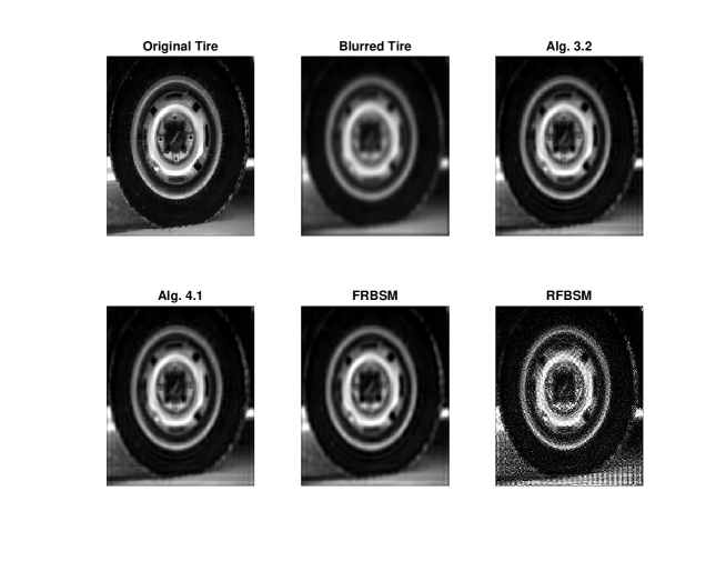
Figure 1. Numerical results for Example 6.1: Top Left: original image; Top Middle: blurred image; Top Right: restored image by Algorithm 3.2 with SNR = 24.7440; Bottom Left: restored image by Algorithm 4.1 with SNR = 24.7440; Bottom Middle: restored image by FRBSM with SNR = 24.4121; Bottom Right: restored image by RFBSM with SNR = 16.6445.

Table 1. Example 6.1: Numerical comparison of Algorithm 3.2, Algorithm 4.1, FRBSM and RFBSM using their SNR values.

Images	$n$	Alg. 3.2	Alg. 4.1	FRBSM	RFBSM
Tire.tif	200	24.4142	24.4142	20.1744	13.8430
($205\times 232$)	500	24.6659	24.6659	22.8918	16.5377
	1000	24.7202	24.7202	23.8513	16.7678
	1500	24.7440	24.7440	24.4121	16.6445

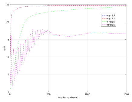
Figure 2. Numerical results for Example 6.1: Showing different SNR for each algorithms.

6.2. Optimal Control Problem

Example 6.2.

Let $\mathfrak{L}^{2}([0,\mathsf{T}],\mathcal{R}^{l})$ be the Hilbert space of all square integrable, measurable vector functions $z:[0,\mathsf{T}]\to\mathcal{R}^{l}$, where $0<\mathsf{T}\in\mathcal{R}$.

We consider the optimal control problem

(6.2) $$z^{*}(t)=\text{argmin}\{\phi(z):z\in\widetilde{Z}\}$$

on the interval $[0,\mathsf{T}]$, where $\widetilde{Z}$ is the set of admissible controls and consists of continuous functions, that is,

$$\widetilde{Z}=\big{\{}z(t)\in\mathfrak{L}^{2}([0,\mathsf{T}],\mathcal{R}^{l}):z_{j}(t)\in[z_{j}^{-},z_{j}^{+}],j=1,2,\ldots,l\big{\}},$$

and the terminal objective has the form

$$\phi(z)=\varphi(w(\mathsf{T})),$$

where $\varphi$ is convex and differentiable on the attainability set and $w(t)$ is a trajectory in $\mathfrak{L}^{2}([0,\mathsf{T}])$.

Assume that this trajectory satisfies the following constraints

$$\dot{w}(t)=\mathcal{P}(t)w(t)+\mathcal{Q}(t)z(t),\quad w(0)=w_{0},\quad t\in[0,\mathsf{T}],$$

where $\mathcal{P}(t)\in\mathcal{R}^{d\times d}$ and $\mathcal{Q}(t)\in\mathcal{R}^{d\times l}$ are continuous matrices for $t\in[0,\mathsf{T}]$.
It follows from the Pontryagin Maximum Principle that there exists $v^{*}\in\mathfrak{L}^{2}([0,\mathsf{T}])$ such that for almost all $t\in[0,\mathsf{T}]$, $(w^{*},v^{*},z^{*})$ solves the system

(6.3) $$\qquad~{}\begin{cases}\begin{aligned} \dot{w}^{*}(t)&=\mathcal{P}(t)w^{*}(t)+\mathcal{Q}(t)z^{*}(t)\\ w^{*}(0)&=x_{0},\\ \end{aligned}\end{cases}$$

(6.4) $$\begin{cases}\begin{aligned} \dot{v}^{*}(t)&=-\mathcal{P}(t)^{\prime}v^{*}(t)\\ v^{*}(\mathsf{T})&=\nabla\varphi(w(\mathsf{T})),\\ \end{aligned}\end{cases}\quad~{}$$

(6.5) $$0\in\mathcal{Q}(t)^{\prime}v^{*}(t)+\mathcal{N}_{\widetilde{Z}}(z^{*}(t)),$$

where $\mathcal{Q}(t)^{\prime}$ means the transpose of $\mathcal{Q}(t)$ and $\mathcal{N}_{\widetilde{Z}}(z)$ is the normal cone to $\widetilde{Z}$ at $z$, which is maximal monotone. Let $Tz(t):=\mathcal{Q}(t)^{\prime}v(t)$. Then $T$ is the gradient of $\phi$ (see [35] and the references therein). Hence (6.5) reduces to the monotone inclusion problem (1.1), where $S=\mathcal{N}_{\widetilde{Z}}$ and $T=\nabla\phi$.

For our computational experiments, we discretize the continuous functions and choose a natural number $K$ with the mesh size $h:=\mathsf{T}/K$. We identify any discretized control $z^{K}:=(z_{0},z_{1},\ldots,z_{K-1})$ with its piecewise constant extension

$$z^{K}(t)=z_{j}~{}\text{for}~{}t\in\left[t_{j},t_{j+1}\right),~{}j=0,1,\ldots K.$$

Also, we identify any discretized state $w^{K}:=(w_{0},w_{1},\ldots,w_{K})$ with its piecewise linear interpolation

$$w^{K}(t)=w_{j}+\frac{t-t_{j}}{h}\left(w_{j+1}-w_{j}\right),~{}\text{for}~{}t\in\left[t_{j},t_{j+1}\right),~{}j=0,1,\ldots,K-1$$

and identify any discretized co-state variable $v^{K}:=(v_{0},v_{1},\ldots,v_{K})$ in a similar manner.
Then we adopt the Euler method for the discretization (see [28, 31, 35] for more details).

Now, consider the following example where the terminal function is nonlinear [4, Example 6.3]:

(6.6) $$\begin{array}[]{ll}\mbox{minimize }&-w_{1}(2)+\left(w_{2}(2)\right)^{2}\\ \mbox{subject to }&\dot{w_{1}}(t)=w_{2}(t),\\ &\dot{w_{2}}(t)=z(t),~{}\forall t\in[0,2],\\ &w_{1}(0)=0,~{}w_{2}(0)=0,\\ &z(t)\in[-1,1].\end{array}$$

The exact optimal control for Problem (6.6) is

$$z^{*}=\begin{cases}\begin{aligned} &1\ &&\mbox{if }\,t\in[0,1.2)\\ -&1&&\mbox{if }\,t\in(1.2,2].\end{aligned}\end{cases}$$

For this example, we take $K=100$ and randomly choose the initial controls in $[-1,1]$. We also take $\delta_{0}=0.1,\delta_{1}=0.3,\bar{r}=0.3,\sigma_{n}=\frac{0.005}{3n+25000},c_{n}=\frac{1}{(n^{2}+1)},\bar{\vartheta}=0.04$ for Algorithms 3.2 and 4.1 while we take $\lambda_{n}=\frac{n+1}{15n+10}$ and $\gamma=0.075$ for FRBSM [21, Algorithm (2.2)] and RFBSM [5, Algorithm (1.6)], respectively. The stopping criterion for this experiment is $\text{Tol}_{n}<10^{-4}$, where $\text{Tol}_{n}=0.5\|w_{n}-J^{S}(w_{n}-Tw_{n})\|^{2}$. Note that ${\text{T}ol}_{n}=0$ implies that $w_{n}\in(T+S)^{-1}(0)$. The numerical results for the experiment are shown in Figure 3.

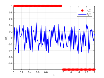
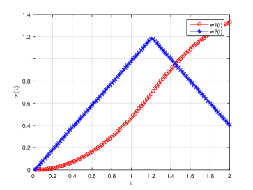
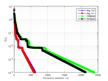
Figure 3. Numerical results for Example 6.2: Top Left: random initial control (blue) and optimal control (red); Top Right: optimal trajectories (Top Left and Top Right computed by Algorithm 3.2); Bottom: comparison of Algorithm 3.2, Algorithm 4.1, FRBSM and RFBSM with CPU time (sec), 1.5656, 1.3799, 4.1210 and 3.6200, respectively.

6.3. Academic Examples

Example 6.3.

Consider the following convex minimization problem:

(6.7) $$\min_{w\in\mathcal{R}^{3}}\|w\|^{2}_{2}+(-7,1,-3)w+4w_{1}+\|w\|_{1},$$

where $w=(w_{1},w_{2},w_{3})\in\mathcal{R}^{3}$.

Set $\mathcal{P}w=\|w\|^{2}_{2}+(-7,1,-3)w+4w_{1}$ and $\mathcal{D}w=\|w\|_{1}$. Then $\mathcal{P}$ is convex and continuously differentiable on $\mathcal{R}^{3}$ with $\nabla\mathcal{P}w=2w+(-3,1,-3)$, and $\mathcal{D}$ is subdifferentiable.
Note that $\nabla\mathcal{P}$ is monotone and $2$-Lipschitz continuous, and $\partial\mathcal{D}$ is maximal monotone, where $\nabla\mathcal{P}$ and $\partial\mathcal{D}$ are the gradient and subdifferential of $\mathcal{P}$ and $\mathcal{D}$, respectively.
Note also that this problem is equivalent to the following inclusion problem:

$$0\in\left(\nabla\mathcal{P}+\partial\mathcal{D}\right)w.$$

It is known that

$$J_{\bar{\delta}}^{S}(w)=(I_{\mathcal{R}^{3}}+\bar{\delta}\partial\mathcal{D})^{-1}(w)=(\mu_{1},\mu_{2},\mu_{3}),$$

where

$$\mu_{i}=\text{sign}(w_{i})\max\{|w_{i}|-\bar{\delta},0\},i=1,2,3.$$

Thus, setting $\nabla\mathcal{P}=T$ and $\partial\mathcal{D}=S$, we can employ our methods to solve the above convex minimization problem.
For the experiment of this example, we choose the same parameters as in Example 6.2. Furthermore, we choose $\hat{v}=(2,1,-6)$ and the initial values as follows:
Case Ia: $w_{0}=(5,1,-4),w_{1}=(20,4,7)$;
Case Ib: $w_{0}=(-7,10,3),w_{1}=(90,-3,-4)$.

The values of the $n$-th iterates $w_{n}$ for each choice of initial values is given in Figure 4 and Table 2 up to $100$ iterations with $D_{n}=0.5\|w_{n}-J^{S}(w_{n}-Tw_{n})\|^{2}$.
Actually, the minimizer of the convex minimization problem (6.7) is $(1,0,1)$ (see Table 2). Thus, we set $\text{Tol}_{n}=0.5\|w_{n}-(1,0,1)\|^{2}$ and use the stopping criterion $\text{Tol}_{n}<10^{-10}$. Furthermore, we plot the graph of $\text{Tol}_{n}$ against number of iterations in Figure 5 with corresponding numerical reports in Table 3.

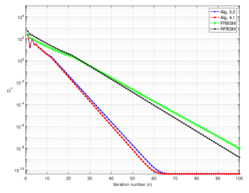
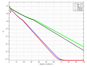
Figure 4. The behavior of $D_{n}$ for Example 6.3: Top Left: Case Ia; Top Right: Case Ib.

Table 2. Numerical results for Example 6.3: Showing different values of the $n$-th iterates $w_{n}$.

	$n$	Alg. 3.2	Alg. 4.1	FRBSM	RFBSM
Ia	10	(2.2949, 0, 1.3516)	(2.2850, 0, 1.3499)	(5.1660, 0.1442, 1.9988)	(5.1808, 0.1348, 2.0915)
	20	(1.1122, 0, 1.0304)	(1.1103, 0, 1.0300)	(2.1861, 0, 1.1284)	(2.0629, 0, 1.2775)
	50	(1.0001, 0, 1.0000)	(1.0001, 0, 1.0000)	(1.0285, 0, 1.0068)	(1.0175, 0, 1.0046)
	70	(1.0000, 0, 1.0000)	(1.0000, 0, 1.0000)	(1.0024, 0, 1.0006)	(1.0011, 0, 1.0003)
	100	(1.0000, 0, 1.0000)	(1.0000, 0, 1.0000)	(1.0001, 0, 1.0000)	(1.0000, 0, 1.0000)
Ib	10	(6.8208, 0, 0.8831)	(6.7805, 0, 0.8829)	(19.1621, 0, 0.6536)	(19.6069, 0, 0.6727)
	20	(1.5042, 0, 0.9899)	(1.4961, 0, 0.9899)	(6.1708, 0, 0.9014)	(5.7306, 0, 0.9168)
	50	(1.0003, 0, 1.0000)	(1.0003, 0, 1.0000)	(1.1243, 0, 0.9976)	(1.0777, 0, 0.9986)
	70	(1.0000, 0, 1.0000)	(1.0000, 0, 1.0000)	(1.0105, 0, 0.9998)	(1.0050, 0, 0.9999)
	100	(1.0000, 0, 1.0000)	(1.0000, 0, 1.0000)	(1.0003, 0, 1.0000)	(1.0000, 0, 1.0000)

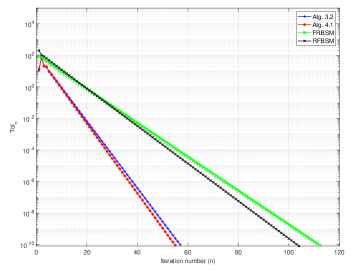
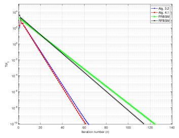
Figure 5. The behavior of $\text{Tol}_{n}$ for Example 6.3: Top Left: Case Ia; Top Right: Case Ib.

Table 3. Numerical results for Example 6.3 with $\text{Tol}_{n}<10^{-10}$.

		Alg. 3.2	Alg. 4.1	FRBSM	RFBSM
Case Ia	CPU time (sec)	0.0024	0.0018	0.0024	0.0036
	No of Iter.	57	55	112	104
Case Ib	CPU time (sec)	0.0033	0.0024	0.0033	0.0790
	No. of Iter.	64	61	124	114

Example 6.4.

Let $\mathcal{H}=\left(\mathfrak{l}_{2}(\mathbb{R}),~{}\|.\|_{\mathfrak{l}_{2}}\right)$, where $\mathfrak{l}_{2}(\mathbb{R}):=\{a=(a_{1},a_{2},...,a_{i},...),~{}~{}a_{i}\in\mathbb{R}:\sum\limits_{i=1}^{\infty}|a_{i}|^{2}<\infty\}$ and $||a||_{\mathfrak{l}_{2}}:=\left(\sum\limits_{i=1}^{\infty}|a_{i}|^{2}\right)^{\frac{1}{2}}\;~{}~{}\forall a\in\mathfrak{l}_{2}(\mathbb{R}).$
Let $S,T:\mathfrak{l}_{2}\to\mathfrak{l}_{2}$ be defined by

$$Sa:=\left(2a_{1},2a_{2},...,2a_{i},...\right),~{}\forall a\in\mathfrak{l}_{2}$$

and

$$Ta:=\left(\frac{a_{1}+|a_{1}|}{2},\frac{a_{2}+|a_{2}|}{2},...,\frac{a_{i}+|a_{i}|}{2},...\right),~{}\forall a\in\mathfrak{l}_{2}.$$

Then $S$ is maximal monotone and $T$ is Lipschitz continuous and monotone with Lipschitz constant $\mathsf{L}=1$.

We choose the following initial values:
Case IIa: $w_{0}=(2,-1,\frac{1}{2},-\frac{1}{4},\dots),w_{1}=(\frac{2}{3},\frac{1}{9},\frac{1}{54},\frac{1}{324},\dots)$;
Case IIb: $w_{0}=(4,1,\frac{1}{4},\frac{1}{16},\dots),w_{1}=(9,3\sqrt{3},3,\sqrt{3},\dots)$;
Case IIc: $w_{0}=(\frac{4}{3},\frac{4}{9},\frac{4}{27},\frac{4}{81},\dots),w_{1}=(-2,1,-\frac{1}{2},\frac{1}{4},\dots)$;
Case IId: $w_{0}=(-4,1,-\frac{1}{4},\frac{1}{16},\dots),w_{1}=(20,-4,\frac{4}{5},-\frac{4}{25},\dots)$.

Also we choose $\delta_{0}=\frac{1}{101},\delta_{1}=\frac{2}{201},\bar{r}=0.15,\hat{v}=(\frac{3}{2},-\frac{3}{4},\frac{3}{8},-\frac{3}{16},\dots),\sigma_{n}=\frac{0.005}{3n+25000},c_{n}=\frac{1}{(10n+77)^{2}},\bar{\vartheta}=0.04$ for Algorithms 3.2 and 4.1 while we take $\lambda_{n}=\frac{n+1}{100n+101}$ and $\gamma=\frac{2}{201}$ for FRBSM [21, Algorithm (2.2)] and RFBSM [5, Algorithm (1.6)], respectively. The stopping criterion for this example is $\text{Tol}_{n}<10^{-8}$, where $\text{Tol}_{n}=0.5\|w_{n}-J^{S}(w_{n}-Tw_{n})\|^{2}$. The numerical results are shown in Figure 6 and Table 4.

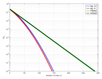
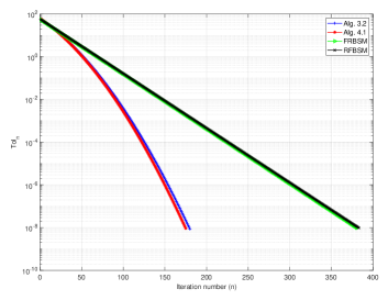
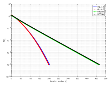
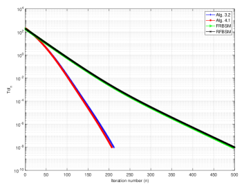
Figure 6. The behavior of $\text{Tol}_{n}$ for Example 6.4: Top Left: Case IIa; Top Right: Case IIb; Bottom Left: Case IIc; Bottom Right: Case IId.

Table 4. Numerical results for Example 6.4 with $\text{Tol}_{n}<10^{-8}$.

		Alg. 3.2	Alg. 4.1	FRBSM	RFBSM
Case IIa	CPU time (sec)	0.0029	0.0027	0.0032	0.0035
	No of Iter.	149	149	288	289
Case IIb	CPU time (sec)	0.0039	0.0034	0.0048	0.0041
	No. of Iter.	180	175	381	383
Case IIc	CPU time (sec)	0.0062	0.0059	0.0071	0.0076
	No of Iter.	203	198	464	466
Case IId	CPU time (sec)	0.0021	0.0019	0.0025	0.0586
	No of Iter.	212	207	498	500

7. Conclusion and future research

We have proposed several new methods for solving the monotone inclusion problem (1.1) in a real Hilbert space. The first method, which we called a forward-reflected-anchored-backward splitting method, inherits the attractive features of the forward-reflected-backward splitting method (1.5), namely, it only involves one forward evaluation of the single-valued operator and one backward evaluation of the set-valued operator, and does not require the cocoercivity of the single-valued operator, but still converges strongly rather than weakly. The other methods of this paper are the inertial, viscosity and inertial viscosity variants of the first one. These variants share the same attractive features of the first method, and they also converge strongly.
Part of our future research is to study the rate of convergence of the proposed methods of this paper.
It would be of interest to incorporate perturbations and error terms to these methods because computing the resolvent of the set-valued operator may be difficult in some applications.
Finally, it would also be of interest to develop anchored (Halpern-type) and viscosity-type variants of the Golden RAtio ALgorithm (GRAAL [18]) for solving the monotone inclusion problem (1.1) and establish their strong convergence.

Declarations

Funding: The second author was partially supported by the Israel Science Foundation (Grant 820/17), by the Fund for the Promotion of Research at the Technion and by the Technion General Research Fund.

Availability of data and material: Not applicable.

Code availability: The Matlab codes employed to run the numerical experiments are available upon request to the authors.

Conflict of interest: The authors declare that they have no known competing financial interests or personal relationships that could have appeared to influence the work reported in this paper.

References

- [1] T.O. Alakoya, L.O. Jolaoso, O.T. Mewomo, Modified inertial subgradient extragradient method with self adaptive stepsize for solving monotone variational inequality and fixed point problems, Optimization, 70 (2021), 545-574.
- [2] J. Bello Cruz, R. Diaz Millan, A variant of forward-backward splitting method for the sum of two monotone operators with a new search strategy, Optimization, 64 (2015), 1471-1486.
- [3] T. Bing, S.Y. Cho, Strong convergence of inertial forward-backward methods for solving monotone inclusions, Appl. Anal., (2021), https://doi.org/10.1080/00036811.2021.1892080
- [4] B. Bressan, B. Piccoli, Introduction to the mathematical theory of control, AIMS Series on Applied Mathematics, (2007)
- [5] V. Cevher, B.C. Vu, A reflected forward-backward splitting method for monotone inclusions involving Lipschitzian operators, Set-Valued Var. Anal., 29 (2021), 163-174.
- [6] G.H. Chen, R.T. Rockafellar, Convergence rates in forward-backward splitting, SIAM J. Optim., 7 (1997), 421-444.
- [7] P. Cholamjiak, D.V. Thong, Y.J. Cho, A novel inertial projection and contraction method for solving pseudomonotone variational inequality problems, Acta Appl. Math., 169 (2020), 217-245.
- [8] J. Diakonikolas, Halpern iteration for near-optimal and parameter-free monotone inclusion and strong solutions to variational inequalities, In Conference on Learning Theory, (2020), 1428-1451.
- [9] A. Gibali, D.V. Thong, Tseng type methods for solving inclusion problems and its applications, Calcolo, 55 (2018), https://doi.org/10.1007/s10092-018-0292-1
- [10] D.V. Hieu, P.K. Anh, L.D. Muu, Modified forward–backward splitting method for variational inclusions, 4OR-Q. J. Oper. Res., 19 (2021), 127-151.
- [11] C. Izuchukwu, S. Reich, Y. Shehu, Relaxed inertial methods for solving the split monotone variational inclusion problem beyond co-coerciveness, Optimization, (2021), https://doi.org/10.1080/02331934.2021.1981895
- [12] C. Izuchukwu, S. Reich, Y. Shehu, Convergence of two simple methods for solving monotone inclusion problems in reflexive Banach spaces, Results Math., 77 (2022), https://doi.org/10.1007/s00025-022-01694-5
- [13] B. Lemaire, Which fixed point does the iteration method select?, Recent Advances in optimization, Springer, Berlin, Germany, 452 (1997), 154-157.
- [14] J.L. Lions, Optimal control of systems governed by partial differential equations. Springer, Berlin (1971)
- [15] P.L. Lions, B. Mercier, Splitting algorithms for the sum of two nonlinear operators, SIAM J. Numer. Anal., 16 (1979), 964-979.
- [16] H. Liu and J. Yang, Weak convergence of iterative methods for solving quasimonotone variational inequalities, Comput. Optim. Appl., 77 (2) (2020), 491-508.
- [17] P.E. Maing, Approximation methods for common fixed points of nonexpansive mappings in Hilbert spaces, J. Math. Anal. Appl., 325 (1) (2007), 469-479.
- [18] Y. Malitsky, Golden ratio algorithms for variational inequalities, Math. Program, 184 (2020), 383-410.
- [19] Y.V. Malitsky; Projected reflected gradient methods for monotone variational inequalities, SIAM J. Optim. 25 (2015), 502-520.
- [20] Y.V. Malitsky, V.V. Semenov, A hybrid method without extrapolation step for solving variational inequality problems, J. Glob. Optim., 61 (2015), 193-202.
- [21] Y. Malitsky and M.K. Tam, A forward-backward splitting method for monotone inclusions without cocoercivity, SIAM J. Optim., 30 (2020), 1451-1472.
- [22] G.B. Passty, Ergodic convergence to a zero of the sum of monotone operators in Hilbert spaces, J. Math. Anal. Appl., 72 (1979), 383-390.
- [23] H. Qi, H.K. Xu, Convergence of Halpern’s iteration method with applications in optimization, Numer. Funct. Anal. Optim. (2021), https://doi.org/10.1080/01630563.2021.2001826
- [24] S. Saejung, P. Yotkaew, Approximation of zeros of inverse strongly monotone operators in Banach spaces, Nonlinear Anal., 75 (2012), 742-750.
- [25] D.R. Sahu, Y.J. Cho, Q.L. Dong, M.R. Kashyap, X.H. Li, Inertial relaxed CQ algorithms for solving a split feasibility problem in Hilbert spaces, Numer Algorithms, 87 (2021), 1075-1095.
- [26] Y. Shehu, X.H. Li, Q.L. Dong, An efficient projection-type method for monotone variational inequalities in Hilbert spaces, Numer. Algorithms, 84 (2020), 365-388.
- [27] Y. Shehu, P.T. Vuong, A. Zemkoho, An inertial extrapolation method for convex simple bilevel optimization, Optim. Methods, Softw., 36 (2021), 1-19.
- [28] Y. Shehu, Q.L. Dong, L. Liu, J.C. Yao, Alternated inertial subgradient extragradient method for equilibrium problems, TOP (2021), https://doi.org/10.1007/s11750-021-00620-2
- [29] R. Suparatulatorn, K. Chaichana, A strongly convergent algorithm for solving common variational inclusion with application to image recovery problems, Appl. Numer. Math. 173 (2022), 239-248.
- [30] S. Takahashi, W. Takahashi, M. Toyoda, Strong convergence theorems for maximal monotone operators with nonlinear mappings in Hilbert spaces, J. Optim Theory Appl., 147 (2010), 27-41.
- [31] B. Tan, X. Qin, J.C. Yao, Strong convergence of inertial projection and contraction methods for pseudomonotone variational inequalities with applications to optimal control problems J. Glob. Optim., 82 (2022), 523-557.
- [32] D.V. Thong, P. Cholamjiak, Strong convergence of a forward-backward splitting method with a new step size for solving monotone inclusions, Comput. Appl. Math. 38 (2019), https://doi.org/10.1007/s40314-019-0855-z.
- [33] Q. Tran-Dinh, Y. Luo, Halpern-type accelerated and splitting algorithms for monotone inclusions, (2021), arXiv:2110.08150v2 [math.OC].
- [34] P. Tseng, A modified forward-backward splitting method for maximal monotone mappings, SIAM J. Control Optim., 38 (2000), 431-446.
- [35] P.T. Vuong, Y. Shehu, Convergence of an extragradient-type method for variational inequality with applications to optimal control problems, Numer. Algorithms, 81 (2019), 269-291.
- [36] Y. Wang, F. Wang, Strong convergence of the forward-backward splitting method with multiple parameters in Hilbert spaces, Optimization, 67 (2018), 493-505.
- [37] T.H. Yoon, E.K. Ryu, Accelerated algorithms for smooth convex-concave minimax problems with rate on squared gradient norm, (2021), arXiv preprint arXiv:2102.07922,