Resolution Guarantees for the Reconstruction of Inclusions in Linear Elasticity Based on Monotonicity Methods

Abstract

We deal with the reconstruction of inclusions in elastic bodies based on monotonicity methods and construct conditions under which a resolution for a given partition can be achieved. These conditions take into account the background error as well as the measurement noise. As a main result, this shows us that the resolution guarantees depend heavily on the Lamé parameter $\mu$ and only marginally on $\lambda$.

Keywords: resolution guarantees, inverse problem, linear elasticity, detection and reconstruction of inclusions, monotonicity methods

1 Introduction

In this paper we deal with the detection and reconstruction of inclusions in elastic bodies based on monotonicity methods, where the main focus lies on the so-called "resolution guarantees". Our results are of special importance, when considering simulations based on real data.

Before we introduce the definition of the resolution guarantees we state the setting. Let $\Omega\subset\mathbb{R}^{d}$ ($d=2$ or $3$) be a bounded and connected open set with Lipschitz boundary $\partial\Omega=\Gamma=\overline{\Gamma_{\mathrm{D}}\cup\Gamma_{\mathrm{N}}}$, $\Gamma_{\mathrm{D}}\cap\Gamma_{\mathrm{N}}=\emptyset$, where $\Gamma_{\textup{D}}$ and $\Gamma_{\textup{N}}$ are the corresponding Dirichlet and Neumann boundaries. We assume that $\Gamma_{\textup{D}}$ and $\Gamma_{\textup{N}}$ are relatively open and connected. Further, $\Omega$ is divided into $N$ disjoint open subsets $(\omega_{s})_{s=1,\ldots,N}$, i.e. a pixel partition, such that $\overline{\Omega}=\bigcup_{s=1,\ldots,N}\overline{\omega_{s}}$.

We base our considerations on the work [16], where the resolution guarantees for the electrical impedance tomography (EIT) problem were considered.

Definition 1.

An inclusion detection method that yields a reconstruction $\mathcal{D}_{R}$ to the true inclusion $\mathcal{D}$ is said to fulfill a resolution guarantee w.r.t. a partition $(\omega_{s})_{s=1,\ldots,N}\subseteq\Omega$ if

• $\omega_{s}\subseteq\mathcal{D}$ implies $\omega_{s}\subseteq\mathcal{D}_{R}$ for $s\in\{1,2,\ldots,N\}$
  (i.e. every element that is covered by the inclusion will be marked in the reconstruction),

• $\mathcal{D}=\emptyset$ implies $\mathcal{D}_{R}=\emptyset$
  (i.e. if there is no inclusion then no element will be marked in the reconstruction).

Remark 1.

Obviously, a reconstruction guarantee will not hold true for arbitrarily fine partitions. The achievable resolution will depend on the number of applied boundary forces, the inclusion contrast, the background error and the measurement noise.

We aim to construct conditions under which a resolution for a given partition can be achieved. These conditions take into account the background error as well as the measurement noise. Thus, we show that it is generally possible to give rigorous guarantees in linear elasticity.

Before we go into more detail about the resolution guarantees, we would like to give an insight into the theory and methods of inclusion detection considered so far.

The theory of the inverse problem of linear elasticity, i.e. uniqueness results and Lipschitz stability studies, etc. were examined, e.g., in the works given below: [23], [25], [29] deal with the 2D case and [18] with two and three dimensions. For uniqueness results in 3D we want to mention [9] and [30, 31] as well as [2, 3] and [25, 28, 30], where some boundary determination results were proved. In addition, results concerning the anisotropic case can be found, e.g., in [19, 21] and [22]. Finally, [20] discussed the reconstruction of inclusion from boundary measurements.

The following methods, among others, were used to solve the inverse problem of linear elasticity: A Landweber iteration method was applied in [17] and [27]. Further on, [24] and [26] considered regularization approaches. Beside the aforementioned methods, adjoint methods were used in [32, 33] and [34]. Further on, [1], [10] and [35] took a look at reciprocity principles. Finally, we want to mention the monotonicity methods for linear elasticity developed by the authors of this paper in [5].

We focus on the monotonicity methods which are built on the examinations in [36, 37]. These methods were first used for EIT (see, e.g., [11, 12, 13, 14, 15]) and then on other problems such as elasticity (see, e.g., [5, 6, 7]). In short, for this method the monotonicity properties of Neumann-to-Dirichlet operator plays an essential role. All in all, this builds the basis for our considerations.

This paper is organized as follows:
First, we introduce the problem statement for linear elasticity and the setting, where we distinguish between the continuous and discrete case. Next, we give a summary of the monotonicity methods, i.e., the standard monotonicity tests as well as the linearized monotonicity tests. In Section 4, we present the background for the resolution guarantees and state the algorithms of the aforementioned monotonicity tests. Further on, we prove the required theorems which build the basis for the algorithms. Finally, we simulate the reconstruction for different settings. As a main result, we conclude that the resolution guarantees depend heavily on the Lamé parameter $\mu$ and only marginally on $\lambda$.

2 Problem Statement and Setting

We take a look at the continuous and discrete setting and introduce the corresponding problems as well the required assumptions concerning the inclusion, the background as well as the measurement error.

2.1 Continuous case

We start with the introduction of the problems of interest, e.g., the direct as well as the inverse problem of stationary linear elasticity.

For the following, we define

$$L_{+}^{\infty}(\Omega):=\{w\in L^{\infty}(\Omega):\underset{x\in\Omega}{\text{ess\,inf}}\,w(x)>0\}.$$

Let $u:\Omega\to\mathbb{R}^{d}$ be the displacement vector, $\mu,\lambda:\Omega\to L^{\infty}_{+}(\Omega)$ the Lamé parameters, $\hat{\nabla}u=\tfrac{1}{2}\left(\nabla u+(\nabla u)^{T}\right)$ the symmetric gradient, $n$ is the normal vector pointing outside of $\Omega$ , $g\in L^{2}(\Gamma_{\textup{N}})^{d}$ the boundary force and $I$ the $d\times d$-identity matrix. We define the divergence of a matrix $A\in\mathbb{R}^{d\times d}$ via $\nabla\cdot A=\sum\limits_{i,j=1}^{d}\dfrac{\partial A_{ij}}{\partial x_{j}}e_{i}$, where $e_{i}$ is a unit vector and $x_{j}$ a component of a vector from $\mathbb{R}^{d}$.
The boundary value problem of linear elasticity (direct problem) is that $u\in H^{1}(\Omega)^{d}$ solves

$$\nabla\cdot\left(\lambda(\nabla\cdot u)I+2\mu\hat{\nabla}u\right) =0\quad\mathrm{in}\,\,\Omega,$$ (1)

$$\left(\lambda(\nabla\cdot u)I+2\mu\hat{\nabla}u\right)n =g\quad\mathrm{on}\,\,\Gamma_{\textup{N}},$$ (2)

$$u =0\quad\mathrm{on}\,\,\Gamma_{\textup{D}}.$$ (3)

From a physical point of view, this means that we deal with an elastic test body $\Omega$ which is fixed (zero displacement) at $\Gamma_{\mathrm{D}}$ (Dirichlet condition) and apply a force $g$ on $\Gamma_{\mathrm{N}}$ (Neumann condition). This results in the displacement $u$, which is measured on the boundary $\Gamma_{\mathrm{N}}$.

The equivalent weak formulation of the boundary value problem (1)-(3) is that $u\in\mathcal{V}$ fulfills

$$\int_{\Omega}2\mu\,\hat{\nabla}u:\hat{\nabla}v+\lambda\nabla\cdot u\,\nabla\cdot v\,dx=\int_{\Gamma_{\textup{N}}}g\cdot v\,ds\quad\text{ for all }v\in\mathcal{V},$$ (4)

where $\mathcal{V}:=\left\{v\in H^{1}(\Omega)^{d}:\,v_{|_{\Gamma_{\textup{D}}}}=0\right\}$.

We want to remark that for $\lambda,\mu\in L^{\infty}_{+}(\Omega)$, the existence and uniqueness of a solution to the variational formulation (4) can be shown by the Lax-Milgram theorem (see e.g., in [4]).

Neumann-to-Dirichlet operator and its monotonicity properties

Measuring boundary displacements that result from applying forces to $\Gamma_{\textup{N}}$ can be modeled by the Neumann-to-Dirichlet operator $\Lambda(\lambda,\mu)$ defined by

$$\Lambda(\lambda,\mu):L^{2}(\Gamma_{\textup{N}})^{d}\rightarrow L^{2}(\Gamma_{\textup{N}})^{d}:\quad g\mapsto u_{|_{\Gamma_{\textup{N}}}},$$

where $u\in\mathcal{V}$ solves (1)-(3).

This operator is self-adjoint, compact and linear (see Corollary 1.1 from [5]). Its associated bilinear form is given by

$$\langle g,\Lambda(\lambda,\mu)h\rangle=\int_{\Omega}2\mu\,\hat{\nabla}u^{g}_{(\lambda,\mu)}:\hat{\nabla}u^{h}_{(\lambda,\mu)}+\lambda\nabla\cdot u^{g}_{(\lambda,\mu)}\,\nabla\cdot u^{h}_{(\lambda,\mu)}\,dx,$$ (5)

where $u_{(\lambda,\mu)}^{g}$ solves the problem (1)-(3) and $u_{(\lambda,\mu)}^{h}$ the corresponding problem with boundary force $h\in L^{2}(\Gamma_{\mathrm{N}})^{d}$.

Another important property of $\Lambda(\lambda,\mu)$ is its Fréchet differentiability (for the corresponding proof see Lemma 2.3 in [5]). For directions $\hat{\lambda},\hat{\mu}\in L^{\infty}(\Omega)$, the derivative

$$\Lambda^{\prime}(\lambda,\mu)(\hat{\lambda},\hat{\mu}):L^{2}(\Gamma_{\textup{N}})^{d}\rightarrow L^{2}(\Gamma_{\textup{N}})^{d}$$

is the self-adjoint compact linear operator associated to the bilinear form

$$\langle\Lambda^{\prime}(\lambda,\mu)(\hat{\lambda},\hat{\mu})g,h\rangle= -\int_{\Omega}2\hat{\mu}\,\hat{\nabla}u^{g}_{(\lambda,\mu)}:\hat{\nabla}u^{h}_{(\lambda,\mu)}+\hat{\lambda}\nabla\cdot u^{g}_{(\lambda,\mu)}\,\nabla\cdot u^{h}_{(\lambda,\mu)}\,dx.$$

Note that for $\hat{\lambda}_{0},\hat{\lambda}_{1},\hat{\mu}_{0},\hat{\mu}_{1}\in L^{\infty}(\Omega)$ with $\hat{\lambda}_{0}\leq\hat{\lambda}_{1}\text{ and }\hat{\mu}_{0}\leq\hat{\mu}_{1}$ we obviously have

$$\Lambda^{\prime}(\lambda,\mu)(\hat{\lambda}_{0},\hat{\mu}_{0})\geq\Lambda^{\prime}(\lambda,\mu)(\hat{\lambda}_{1},\hat{\mu}_{1}),$$ (6)

in the sense of quadratic forms.

The inverse problem we consider here is the following:

$$\text{ \it Find the support of }(\lambda-\lambda_{0},\mu-\mu_{0})^{T}\text{ \it knowing the Neumann-to-Dirichlet operator }\Lambda(\lambda,\mu).$$

2.2 Discrete case

Next, we go over to the discrete case and take a look at the bounded domain $\Omega\subset\mathbb{R}^{d}$ with piecewise smooth boundary representing the elastic object. Further on, let $\lambda,\mu:\Omega\to\mathbb{R}^{+}$ be the real valued Lamé parameter distribution inside $\Omega$.

We apply the forces $g_{l}$ on the Neumann boundary of the object, where the location of their support is denoted by $\Gamma_{\mathrm{N}}^{(l)}\subseteq\Gamma_{\mathrm{N}}$, $l=1,\ldots,M$. We assume that the patches are disjoint. Thus, the discrete boundary value problem is given by

$$\nabla\cdot\left(\lambda(\nabla\cdot u)I+2\mu\hat{\nabla}u\right) =0\,\,\quad\text{in}\,\,\Omega,$$ (7)

$$\left(\lambda(\nabla\cdot u)I+2\mu\hat{\nabla}u\right)n =g_{l}\quad\text{on}\,\,\Gamma_{\mathrm{N}}^{(l)},$$ (8)

$$\left(\lambda(\nabla\cdot u)I+2\mu\hat{\nabla}u\right)n =0\quad\text{on}\,\,\Gamma_{\mathrm{N}}^{(i)},\,i\neq l,$$ (9)

$$u =0\,\,\quad\text{in}\,\,\Gamma_{\mathrm{D}}.$$ (10)

The resulting displacement measurements are represented by the discrete version of $\Lambda(\lambda,\mu)$:

$${\bm{\Lambda}}(\lambda,\mu)=\left(\Lambda_{l}^{(k)}(\lambda,\mu)\right)_{k,l=1,\ldots,M}$$ (11)

with

$$\Lambda_{l}^{(k)}(\lambda,\mu):=\int_{\Gamma_{\mathrm{N}}^{(l)}}g_{l}\cdot u^{(k)}\,ds$$

and $u^{(k)}$ solves the boundary value problem (7)-(10) for a boundary load $g_{k}$.

Assumptions regarding the inclusion, the background as well as the measurement error

In the following, we introduce our assumptions and definitions concerning the Lamé parameters for the inclusion and background including their error considerations.

• Distribution of Lamé parameter $(\lambda(x),\mu(x))$:

  $$(\lambda(x),\mu(x))=\begin{cases}(\lambda_{\mathcal{D}}(x),\mu_{\mathcal{D}}(x)),&\quad x\in\mathcal{D},\\ (\lambda_{\mathcal{B}}(x),\mu_{\mathcal{B}}(x)),&\quad x\in\Omega\setminus\mathcal{D},\end{cases}$$

  where $\mathcal{D}$ denotes the unknown inclusion and $\mathcal{B}$ the background.

• Background error $\epsilon^{\lambda},\epsilon^{\mu}\geq 0$:

  $$|(\lambda_{\mathcal{B}}(x),\mu_{\mathcal{B}}(x))-(\lambda_{0},\mu_{0})|\leq(\lambda_{0}\epsilon^{\lambda},\mu_{0}\epsilon^{\mu})\quad\text{for all}\,x\in\Omega\setminus\mathcal{D},$$

  where the background Lamé parameters $\lambda_{\mathcal{B}}(x)$ and $\mu_{\mathcal{B}}(x)$ approximately agree with known positive constants $\lambda_{0}$ and $\mu_{0}$.

• Inclusion contrast $c^{\lambda},c^{\mu}>0$:
  We distinguish between the following two cases

  either $(\lambda_{\mathcal{D}}(x),\mu_{\mathcal{D}}(x))-(\lambda_{0},\mu_{0})\geq(c^{\lambda},c^{\mu})\,\,\text{for all}\,x\in\mathcal{D}$
   or $\quad\,\,\,\,(\lambda_{0},\mu_{0})-(\lambda_{\mathcal{D}}(x),\mu_{\mathcal{D}}(x))\geq(c^{\lambda},c^{\mu})\,\,\text{for all}\,x\in\mathcal{D}$,
  
  where the lower bounds $c^{\lambda}$ and $c^{\mu}$ are known.

• Measurement noise $\delta\geq 0$:

  $$||{\bm{\Lambda}}(\lambda,\mu)-{\bm{\Lambda}}^{\delta}(\lambda,\mu)||\leq\delta,$$

  i.e., we assume that ${\bm{\Lambda}(\lambda,\mu)}$ is determined up to noise level $\delta>0$.

3 Summary of the Monotonicity Methods

First, we state the monotonicity estimates for the Neumann-to-Dirichlet operator $\Lambda(\lambda,\mu)$ and denote by $u^{g}_{(\lambda,\mu)}$ the solution of problem (1)-(3) for the boundary load $g$ and the Lamé parameters $\lambda$ and $\mu$.

Lemma 1 (Lemma 3.1 from [7]).

Let $(\lambda_{1},\mu_{1}),(\lambda_{2},\mu_{2})\in L_{+}^{\infty}(\Omega)\times L_{+}^{\infty}(\Omega)$, $g\in L^{2}(\Gamma_{\textup{N}})^{d}$ be an applied boundary force, and let $u_{1}:=u^{g}_{(\lambda_{1},\mu_{1})}\in\mathcal{V}$, $u_{2}:=u^{g}_{(\lambda_{2},\mu_{2})}\in\mathcal{V}$. Then

$$\int_{\Omega} 2(\mu_{1}-\mu_{2})\hat{\nabla}u_{2}:\hat{\nabla}u_{2}+(\lambda_{1}-\lambda_{2})\nabla\cdot u_{2}\nabla\cdot u_{2}\,dx$$ (12)

$$\geq\langle g,\Lambda(\lambda_{2},\mu_{2})g\rangle-\langle g,\Lambda(\lambda_{1},\mu_{1})g\rangle$$

$$\geq\int_{\Omega}2(\mu_{1}-\mu_{2})\hat{\nabla}u_{1}:\hat{\nabla}u_{1}+(\lambda_{1}-\lambda_{2})\nabla\cdot u_{1}\nabla\cdot u_{1}\,dx.$$ (13)

Lemma 2 (Lemma 2 from [5]).

Let $(\lambda_{1},\mu_{1}),(\lambda_{2},\mu_{2})\in L_{+}^{\infty}(\Omega)\times L_{+}^{\infty}(\Omega)$, $g\in L^{2}(\Gamma_{\textup{N}})^{d}$ be an applied boundary force, and let $u_{1}:=u^{g}_{(\lambda_{1},\mu_{1})}\in\mathcal{V}$, $u_{2}:=u^{g}_{(\lambda_{2},\mu_{2})}\in\mathcal{V}$. Then

$$\langle g ,\Lambda(\lambda_{2},\mu_{2})g\rangle-\langle g,\Lambda(\lambda_{1},\mu_{1})g\rangle$$ (14)

$$\geq\int_{\Omega}2\left(\mu_{2}-\frac{\mu_{2}^{2}}{\mu_{1}}\right)\hat{\nabla}u_{2}:\hat{\nabla}u_{2}\,dx+\int_{\Omega}\left(\lambda_{2}-\frac{\lambda_{2}^{2}}{\lambda_{1}}\right)\nabla\cdot u_{2}\nabla\cdot u_{2}\,dx$$

$$=\int_{\Omega}2\frac{\mu_{2}}{\mu_{1}}\left(\mu_{1}-\mu_{2}\right)\hat{\nabla}u_{2}:\hat{\nabla}u_{2}\,dx+\int_{\Omega}\frac{\lambda_{2}}{\lambda_{1}}\left(\lambda_{1}-\lambda_{2}\right)\nabla\cdot u_{2}\nabla\cdot u_{2}\,dx.$$ (15)

Corollary 1 (Corollary 3.2 from [7]).

For $(\lambda_{0},\mu_{0}),(\lambda_{1},\mu_{1})\in L_{+}^{\infty}(\Omega)\times L_{+}^{\infty}(\Omega)$

$$\lambda_{0}\leq\lambda_{1}\text{ and }\mu_{0}\leq\mu_{1}\quad\text{ implies }\quad\Lambda(\lambda_{0},\mu_{0})\geq\Lambda(\lambda_{1},\mu_{1}).$$ (16)

We give a short overview concerning the monotonicity methods, where we restrict ourselves to the case $\lambda_{1}\geq\lambda_{0}$, $\mu_{1}\geq\mu_{0}$. In the following, let $\mathcal{D}$ be the unknown inclusion and $\chi_{\mathcal{D}}$ the characteristic function w.r.t. $\mathcal{D}$. In addition, we deal with "noisy difference measurements", i.e. distance measurements between $u^{g}_{(\lambda,\mu)}$ and $u^{g}_{(\lambda_{0},\mu_{0})}$ affected by noise, which stem from the corresponding system (1)-(3).

We define the outer support in correspondence to [5] as follows: let $\phi=(\phi_{1},\phi_{2}):\Omega\to\mathbb{R}^{2}$ be a measurable function, the outer support $\underset{\partial\Omega}{\mathrm{out}}\,\mathrm{supp}(\phi)$ is the complement (in $\overline{\Omega}$) of the union of those relatively open $U\subseteq\overline{\Omega}$ that are connected to $\partial\Omega$ and for which $\phi|_{U}=0$, respectively.

3.1 Standard Monotonicity Tests

We start our consideration with the standard monotonicity tests and take a look at the case for exact as well as noisy data. Here, we denote the material without inclusion by $(\lambda_{0},\mu_{0})$ and the Lamé parameters of the inclusion by $(\lambda_{1},\mu_{1})$.

Tests for exact and noisy data

Corollary 2.

Standard monotonicity test (Corollary 2.4 from [5])
Let $\lambda_{0},\lambda_{1},\mu_{0},\mu_{1}\in\mathbb{R}^{+}$, $(\lambda,\mu)=(\lambda_{0}+(\lambda_{1}-\lambda_{0})\chi_{\mathcal{D}},\mu_{0}+(\mu_{1}-\mu_{0})\chi_{\mathcal{D}})$ with $\lambda_{1}>\lambda_{0}$ and $\mu_{1}>\mu_{0}$ and the inclusion $\mathcal{D}=\mathrm{out}_{\partial\Omega}\,\mathrm{supp}((\lambda-\lambda_{0},\mu-\mu_{0})^{T})$. Further on, let $\alpha^{\lambda},\alpha^{\mu}\geq 0$, $\alpha^{\lambda}+\alpha^{\mu}>0$ with $\alpha^{\lambda}\leq\lambda_{1}-\lambda_{0}$, $\alpha^{\mu}\leq\mu_{1}-\mu_{0}$. Then for every open set $\omega\subseteq\Omega$

$$\omega\subseteq\mathcal{D}\quad\text{if\,and\,only\,if}\quad\Lambda(\lambda_{0}+\alpha^{\lambda}\chi_{\omega},\mu_{0}+\alpha^{\mu}\chi_{\omega})\geq\Lambda(\lambda,\mu).$$

Corollary 3.

Standard monotonicity test for noisy data (Corollary 2.6 from [5])
Let $\lambda_{0},\lambda_{1},\mu_{0},\mu_{1}\in\mathbb{R}^{+}$, $(\lambda,\mu)=(\lambda_{0}+(\lambda_{1}-\lambda_{0})\chi_{\mathcal{D}},\mu_{0}+(\mu_{1}-\mu_{0})\chi_{\mathcal{D}})$ with $\lambda_{1}>\lambda_{0}$ and $\mu_{1}>\mu_{0}$ and the inclusion $\mathcal{D}=\mathrm{out}_{\partial\Omega}\,\mathrm{supp}((\lambda-\lambda_{0},\mu-\mu_{0})^{T})$. Further on, let $\alpha^{\lambda}\,\alpha^{\mu}\geq 0$, $\alpha+\beta>0$ with $\alpha^{\lambda}\leq\lambda_{1}-\lambda_{0}$, $\alpha^{\mu}\leq\mu_{1}-\mu_{0}$ and let each noise level $\delta>0$ fulfill

$$\|{\Lambda^{\delta}(\lambda,\mu)-\Lambda(\lambda,\mu)}\|<\delta.$$

Then for every open set $\omega\subseteq\Omega$ there exists a noise level $\delta_{0}>0$, such that $\omega$ is correctly detected as inside the inclusion $\mathcal{D}$ by the condition

$$\omega\subseteq\mathcal{D}\quad\textnormal{ if and only if}\quad\Lambda(\lambda_{0}+\alpha^{\lambda}\chi_{\omega},\mu_{0}+\alpha^{\mu}\chi_{\omega})-\Lambda^{\delta}(\lambda,\mu)+\delta I\geq 0$$

for all $\quad 0<\delta<\delta_{0}$.

3.2 Linearized Monotonicity Tests

We also introduce the linearized monotonicity tests as a modification of the standard methods. Similar as before, we deal with the exact as well as perturbed problem.

Tests for exact and noisy data

Corollary 4.

Linearized monotonicity test (Corollary 2.7 from [5])
Let $\lambda_{0}$, $\lambda_{1}$, $\mu_{0}$, $\mu_{1}\in\mathbb{R}^{+}$ with $\lambda_{1}>\lambda_{0}$, $\mu_{1}>\mu_{0}$ and assume that $(\lambda,\mu)=(\lambda_{0}+(\lambda_{1}-\lambda_{0})\chi_{\mathcal{D}},\mu_{0}+(\mu_{1}-\mu_{0})\chi_{\mathcal{D}})$ with $\mathcal{D}=\mathrm{out}_{\partial\Omega}\,\mathrm{supp}((\lambda-\lambda_{0},\mu-\mu_{0})^{T})$. Further on let $\alpha^{\lambda},\alpha^{\mu}\geq 0$, $\alpha^{\lambda}+\alpha^{\mu}>0$ and $\alpha^{\lambda}\leq\tfrac{\lambda_{0}}{\lambda_{1}}(\lambda_{1}-\lambda_{0})$, $\alpha^{\mu}\leq\tfrac{\mu_{0}}{\mu_{1}}(\mu_{1}-\mu_{0})$. Then for every open set $\omega$

$$\omega\subseteq\mathcal{D}\quad\text{if and only if}\quad\Lambda(\lambda_{0},\mu_{0})+\Lambda^{\prime}(\lambda_{0},\mu_{0})(\alpha^{\lambda}\chi_{\omega},\alpha^{\mu}\chi_{\omega})\geq\Lambda(\lambda,\mu).$$

Corollary 5.

Linearized monotonicity test for noisy data (Corollary 2.9 from [5])
Let $\lambda_{0}$, $\lambda_{1}$, $\mu_{0}$, $\mu_{1}\in\mathbb{R}^{+}$ with $\lambda_{1}>\lambda_{0}$, $\mu_{1}>\mu_{0}$ and assume that $(\lambda,\mu)=(\lambda_{0}+(\lambda_{1}-\lambda_{0})\chi_{\mathcal{D}},\mu_{0}+(\mu_{1}-\mu_{0})\chi_{\mathcal{D}})$ with $\mathcal{D}=\mathrm{out}_{\partial\Omega}\,\mathrm{supp}((\lambda-\lambda_{0},\mu-\mu_{0})^{T})$. Further on, let $\alpha^{\lambda},\alpha^{\mu}\geq 0$, $\alpha^{\lambda}+\alpha^{\mu}>0$ with $\alpha^{\lambda}\leq\frac{\lambda_{0}}{\lambda_{1}}(\lambda_{1}-\lambda_{0})$, $\alpha^{\mu}\leq\frac{\mu_{0}}{\mu_{1}}(\mu_{1}-\mu_{0})$. Let $\Lambda^{\delta}$ be the Neumann-to-Dirichlet operator for noisy difference measurements with noise level $\delta>0$. Then for every open set $\omega\subseteq\Omega$ there exists a noise level $\delta_{0}>0$, such that for all $0<\delta<\delta_{0}$, $\omega$ is correctly detected as inside or not inside the inclusion $\mathcal{D}$ by the following monotonicity test

$$\omega\subseteq\mathcal{D}\quad\textnormal{\it if and only if}\quad\Lambda(\lambda_{0},\mu_{0})+\Lambda^{\prime}(\lambda_{0},\mu_{0})(\alpha^{\lambda}\chi_{\omega},\alpha^{\mu}\chi_{\omega})-\Lambda^{\delta}(\lambda,\mu)+\delta I\geq 0.$$

4 Resolution Guarantees

In this section we formulate the algorithms for the monotonicity tests, i.e., the standard monotonicity tests as well as the linearized tests and follow the considerations in [16], where resolution guarantees for EIT were analysed.

4.1 Algorithms

Before we take a look at the algorithms for the reconstruction, we define the corresponding notations which we will use in the following. We set

$$(\lambda_{\mathcal{B}_{\min}},\mu_{\mathcal{B}_{\min}}) :=(\lambda_{0}(1-\epsilon^{\lambda}),\mu_{0}(1-\epsilon^{\mu})),$$

$$(\lambda_{\mathcal{B}_{\max}},\mu_{\mathcal{B}_{\max}}) :=(\lambda_{0}(1+\epsilon^{\lambda}),\mu_{0}(1+\epsilon^{\mu})),$$

$$(\lambda_{\mathcal{D}_{\min}},\mu_{\mathcal{D}_{\min}}) :=(\lambda_{0}+c^{\lambda},\mu_{0}+c^{\mu}),$$

$$(\lambda_{\mathcal{D}_{\max}},\mu_{\mathcal{D}_{\max}}) :=(\lambda_{0}-c^{\lambda},\mu_{0}-c^{\mu}),$$

where the quantities are given in Subsection 2.2 assumptions (a)-(d).

4.1.1 Algorithms for standard monotonicity tests

We now formulate the algorithms for the standard monotonicity tests. We start with the case that

$$\left(\lambda_{\mathcal{D}_{\min}},\mu_{\mathcal{D}_{\min}}\right)>(\lambda_{\mathcal{B}_{\max}},\mu_{\mathcal{B}_{\max}})$$

and it holds that

$$\left(\lambda_{\mathcal{D}}-\lambda_{0},\mu_{\mathcal{D}}-\mu_{0}\right)\geq\left(c^{\lambda},c^{\mu}\right).$$

Algorithm 1.

Mark each resolution element $\omega_{s}$ for which

$${\bm{\Lambda}}\left(\tau_{s}^{\lambda},\tau_{s}^{\mu}\right)+\delta{\bf I}\geq{\bm{\Lambda}}^{\delta}(\lambda,\mu),\quad s\in\{1,2,\ldots,N\},$$

where

$$\tau_{s}^{\lambda} :=\lambda_{\mathcal{B}_{\min}}\chi_{\Omega\setminus\omega_{s}}+\lambda_{\mathcal{D}_{\min}}\chi_{\omega_{s}},$$

$$\tau_{s}^{\mu} :=\mu_{\mathcal{B}_{\min}}\chi_{\Omega\setminus\omega_{s}}+\mu_{\mathcal{D}_{\min}}\chi_{\omega_{s}}.$$

Then the reconstruction $\mathcal{D}_{R}$ is given by the union of the marked resolution elements.

Further on, we take a look at the special case for "weaker" Lamé parameter inclusions and consider the case

$$(\lambda_{\mathcal{D}_{\max}},\mu_{\mathcal{D}_{\max}})<(\lambda_{\mathcal{B}_{\min}},\mu_{\mathcal{B}_{\min}}).$$ (17)

Algorithm 2.

Mark each resolution element $\omega_{s}$ for which

$${\bm{\Lambda}}\left(\tau_{s}^{\lambda},\tau_{s}^{\mu}\right)-\delta{\bf I}\leq{\bm{\Lambda}}^{\delta}(\lambda,\mu),\quad s\in\{1,2,\ldots,N\},$$

where

$$\tau_{s}^{\lambda} :=\lambda_{\mathcal{B}_{\max}}\chi_{\Omega\setminus\omega_{s}}+\lambda_{\mathcal{D}_{\max}}\chi_{\omega_{s}},$$

$$\tau_{s}^{\mu} :=\mu_{\mathcal{B}_{\max}}\chi_{\Omega\setminus\omega_{s}}+\mu_{\mathcal{D}_{\max}}\chi_{\omega_{s}}.$$

4.1.2 Algorithms for linearized monotonicity tests

Replacing the monotonicity test for the case $\left(\lambda_{\mathcal{D}_{\min}},\mu_{\mathcal{D}_{\min}}\right)>(\lambda_{\mathcal{B}_{\max}},\mu_{\mathcal{B}_{\max}})$, i.e.

$${\bm{\Lambda}}\left(\tau_{s}^{\lambda},\tau_{s}^{\mu}\right)+\delta{\bf I}\geq{\bm{\Lambda}}^{\delta}(\lambda,\mu)$$

with their linearized approximations yields the linearized monotonicity test

$${\bm{\Lambda}}\left(\lambda_{\mathcal{B}_{\min}},\mu_{\mathcal{B}_{\min}}\right)+{\bm{\Lambda}}^{\prime}\left(\lambda_{\mathcal{B}_{\min}},\mu_{\mathcal{B}_{\min}}\right)(\kappa^{\lambda}\chi_{\omega_{s}},\kappa^{\mu}\chi_{\omega_{s}})+\delta{\bf I}\geq{\bm{\Lambda}}^{\delta}(\lambda,\mu),$$

where $\kappa^{\lambda},\kappa^{\mu}\in\mathbb{R}$ is a suitable contrast level defined in the following algorithm. Further, we assume the $\lambda_{\max}$ and $\mu_{\max}$ are global bounds with

$$\lambda(x) \leq\lambda_{\max},$$

$$\mu(x) \leq\mu_{\max}$$

for all $x\in\Omega$.

Algorithm 3.

Mark each resolution element $\omega_{s}$ for which

$${\bf T}_{s}+\delta{\bf I}\geq{\bm{\Lambda}}^{\delta}(\lambda,\mu),$$

where

$${\bf T}_{s}:={\bm{\Lambda}}\left(\lambda_{\mathcal{B}_{\min}},\mu_{\mathcal{B}_{\min}}\right)+{\bm{\Lambda}}^{\prime}\left(\lambda_{\mathcal{B}_{\min}},\mu_{\mathcal{B}_{\min}}\right)(\kappa^{\lambda}\chi_{\omega_{s}},\kappa^{\mu}\chi_{\omega_{s}}),$$

with

$$\kappa^{\lambda} :=(c^{\lambda}+\lambda_{0}\epsilon^{\lambda})\dfrac{\lambda_{\mathcal{B}_{\min}}}{\lambda_{\max}},$$ (18)

$$\kappa^{\mu} :=(c^{\mu}+\mu_{0}\epsilon^{\mu})\dfrac{\mu_{\mathcal{B}_{\min}}}{\mu_{\max}}.$$ (19)

Then the reconstruction $\mathcal{D}_{R}$ is given by the union of the marked resolution elements.

As for the standard monotonicity test, we formulate the linearized test for inclusions with weaker Lamé parameter which fulfill $(\lambda_{\mathcal{D}_{\max}},\mu_{\mathcal{D}_{\max}})<(\lambda_{\mathcal{B}_{\min}},\mu_{\mathcal{B}_{\min}})$.

Algorithm 4.

Mark each resolution element $\omega_{s}$ for which

$${\bf T}_{s}-\delta{\bf I}\leq{\bm{\Lambda}}^{\delta}(\lambda,\mu),$$

where

$${\bf T}_{s}:={\bm{\Lambda}}\left(\lambda_{\mathcal{B}_{\max}},\mu_{\mathcal{B}_{\max}}\right)+{\bm{\Lambda}}^{\prime}\left(\lambda_{\mathcal{B}_{\max}},\mu_{\mathcal{B}_{\max}}\right)(\kappa^{\lambda}\chi_{\omega_{s}},\kappa^{\mu}\chi_{\omega_{s}})$$

with

$$\kappa^{\lambda} :=-(c^{\lambda}+\lambda_{0}\epsilon^{\lambda}),$$ (20)

$$\kappa^{\mu} :=-(c^{\mu}+\mu_{0}\epsilon^{\mu})$$ (21)

for $s\in\{1,2,\ldots,N\}$.

Then the reconstruction $\mathcal{D}_{R}$ is given by the union of the marked resolution elements.

4.2 Formulation of theorems

We will analyse the algorithms in more detail and take a look at the required theorems.

4.2.1 Theorems for standard monotonicity tests

Theorem 1.

The reconstruction of Algorithm 1 fulfills the resolution guarantees if

$$\nu<-2\delta\leq 0$$

with

$$\nu:=\max_{s=1,\ldots,N}\left(\min\left(\mathrm{eig}\left[{\bm{\Lambda}}\left(\tau_{s}^{\lambda},\tau_{s}^{\mu}\right)-{\bm{\Lambda}}(\lambda_{\mathcal{B}_{\max}},\mu_{\mathcal{B}_{\max}})\right]\right)\right).$$

Proof.

We start with the consideration of part (i) from Definition 1 and let $\omega_{s}\subseteq\mathcal{D}$. Then

$$(\tau_{s}^{\lambda},\tau_{s}^{\mu})=\left(\lambda_{\mathcal{B}_{\min}}\chi_{\Omega\setminus\omega_{s}}+\lambda_{\mathcal{D}_{\min}}\chi_{\omega_{s}},\mu_{\mathcal{B}_{\min}}\chi_{\Omega\setminus\omega_{s}}+\mu_{\mathcal{D}_{\min}}\chi_{\omega_{s}}\right)\leq(\lambda,\mu).$$

The knowledge, that from $(\lambda_{1},\mu_{1})\leq(\lambda_{2},\mu_{2})$ it follows that

$${\bm{\Lambda}}(\lambda_{1},\mu_{1})\geq{\bm{\Lambda}}(\lambda_{2},\mu_{2}),$$ (22)

implies that

$${\bm{\Lambda}}\left(\tau_{s}^{\lambda},\tau_{s}^{\mu}\right)\geq{\bm{\Lambda}}(\lambda,\mu).$$

Hence,

$${\bm{\Lambda}}\left(\tau_{s}^{\lambda},\tau_{s}^{\mu}\right)+\delta{\bf I}\geq{\bm{\Lambda}}^{\delta}(\lambda,\mu),$$

so that $\omega_{s}$ will be marked by the algorithm.
This shows that part (i) of the resolution guarantee is satisfied.

To prove part (ii) of the resolution guarantee, assume that $\mathcal{D}=\emptyset$ and $\mathcal{D}_{R}\neq\emptyset$. Then there must be an index $s\in\{1,2,\ldots,N\}$ with

$${\bm{\Lambda}}\left(\tau_{s}^{\lambda},\tau_{s}^{\mu}\right)+\delta{\bf I}\geq{\bm{\Lambda}}^{\delta}(\lambda,\mu).$$

Again, with the monotonicity relation (22), we obtain

$$-2\delta{\bf I} \leq{\bm{\Lambda}}\left(\tau_{s}^{\lambda},\tau_{s}^{\mu}\right)-\left(\delta{\bf I}+{\bm{\Lambda}}^{\delta}(\lambda,\mu)\right)$$

$$\leq{\bm{\Lambda}}\left(\tau_{s}^{\lambda},\tau_{s}^{\mu}\right)-{\bm{\Lambda}}(\lambda,\mu)$$

$$\leq{\bm{\Lambda}}\left(\tau_{s}^{\lambda},\tau_{s}^{\mu}\right)-{\bm{\Lambda}}(\lambda_{\mathcal{B}_{\max}},\mu_{\mathcal{B}_{\max}})$$

and thus $\nu\geq-2\delta$, which is a contradiction. ∎

All in all, this theorem gives a rigorous yet conceptually simple criterion to check whether a given resolution guarantee is valid or not.

Remark 2.

Given a partition $\left(\omega_{s}\right)_{s=1,\ldots,N}$ and bounds on the background, we obtain $\nu$ from calculating

$${\bm{\Lambda}}\left(\tau_{s}^{\lambda},\tau_{s}^{\mu}\right)\quad\text{and}\quad{\bm{\Lambda}}(\lambda_{\mathcal{B}_{\max}},\mu_{\mathcal{B}_{\max}})$$

by solving the boundary value problem (7)-(10). If this yields a negative value for $\nu$, then the resolution guarantee holds true up to a measurement error of $\delta<-\dfrac{\nu}{2}$.

Next, we formulate the corresponding theorem for case (17).

Theorem 2.

The reconstruction of Algorithm 2 fulfills the resolution guarantee if

$$\nu>2\delta\geq 0$$

with

$$\nu:=\min_{s=1,\ldots,N}\left(\max\left(\mathrm{eig}\left[{\bm{\Lambda}}\left(\tau_{s}^{\lambda},\tau_{s}^{\mu}\right)-{\bm{\Lambda}}(\lambda_{\mathcal{B}_{\min}},\mu_{\mathcal{B}_{\min}})\right]\right)\right).$$

Proof.

The proof of part (i) of the resolution guarantee is analogous to the proof of part (i) in the theorem before.
To show part (ii) of the resolution guarantee, assume that $\mathcal{D}=\emptyset$ and $\mathcal{D}_{R}\neq\emptyset$. Then there must be an index $s\in\{1,2\ldots,N\}$ with

$${\bm{\Lambda}}\left(\tau_{s}^{\lambda},\tau_{s}^{\mu}\right)-\delta{\bf I}$$

$$\leq{\bm{\Lambda}}^{\delta}(\lambda,\mu)$$

$$\leq{\bm{\Lambda}}(\lambda,\mu)+\delta{\bf I}.$$

Using the results from before, we obtain

$${\bm{\Lambda}}\left(\tau_{s}^{\lambda},\tau_{s}^{\mu}\right)-2\delta{\bf I}$$

$$\leq{\bm{\Lambda}}(\lambda_{\mathcal{B}_{\min}},\mu_{\mathcal{B}_{\min}})$$

and thus $\nu\geq 2\delta$, which is a contradiction. ∎

4.2.2 Theorems for linearized monotonicity tests

Theorem 3.

The reconstruction of Algorithm 3 fulfills the resolution guarantee if

$$\nu<-2\delta\leq 0$$

with

$$\nu:=\max_{s=1,\ldots,N}\left(\min\left(\mathrm{eig}\left[{\bf T}_{s}-{\bm{\Lambda}}(\lambda_{\mathcal{B}_{\max}},\mu_{\mathcal{B}_{\max}})\right]\right)\right).$$

Proof.

First, let $\omega_{s}\subseteq\mathcal{D}$ and let $g_{j}\in\mathbb{R}^{M}$, $j\in\{1,2,\ldots,N\}$. In a body with interior Lamé parameters $(\lambda_{\mathcal{B}_{\min}},\mu_{\mathcal{B}_{\min}})$, let $u_{g_{j}}$ be the corresponding displacements resulting from applying the boundary load $g_{j}$ to the $j$-th patch.

$$g_{j}^{T}\left({\bm{\Lambda}}(\lambda_{\mathcal{B}_{\min}},\mu_{\mathcal{B}_{\min}})-{\bm{\Lambda}}(\lambda,\mu)\right)g_{j}$$

$$\geq\int_{\Omega}\dfrac{\lambda_{\mathcal{B}_{\min}}}{\lambda}(\lambda-\lambda_{\mathcal{B}_{\min}})\nabla\cdot u_{g_{j}}\nabla\cdot u_{g_{j}}+2\dfrac{\mu_{\mathcal{B}_{\min}}}{\mu}(\mu-\mu_{\mathcal{B}_{\min}})\hat{\nabla}u_{g_{j}}:\hat{\nabla}u_{g_{j}}\,dx$$

and since $\omega_{s}\subseteq\mathcal{D}$ implies $\lambda-\lambda_{\mathcal{B}_{\min}}\geq(c^{\lambda}+\lambda_{0}\epsilon^{\lambda})\chi_{\omega_{s}}$ and $\mu-\mu_{\mathcal{B}_{\min}}\geq(c^{\mu}+\mu_{0}\epsilon^{\mu})\chi_{\omega_{s}}$, it follows that

$${\bm{\Lambda}}(\lambda_{\mathcal{B}_{\min}},\mu_{\mathcal{B}_{\min}})-{\bm{\Lambda}}(\lambda,\mu)\geq-{\bm{\Lambda}}^{\prime}(\lambda_{\mathcal{B}_{\min}},\mu_{\mathcal{B}_{\min}})(\kappa^{\lambda}\chi_{\omega_{s}},\kappa^{\mu}\chi_{\omega_{s}}).$$

Hence, we obtain that

$${\bf T}_{s}+\delta{\bf I}$$

$$={\bm{\Lambda}}(\lambda_{\mathcal{B}_{\min}},\mu_{\mathcal{B}_{\min}})+{\bm{\Lambda}}^{\prime}(\lambda_{\mathcal{B}_{\min}},\mu_{\mathcal{B}_{\min}})(\kappa^{\lambda}\chi_{\omega_{s}},\kappa^{\mu}\chi_{\omega_{s}})+\delta{\bf I}$$

$$\geq{\bm{\Lambda}}(\lambda,\mu)+\delta{\bf I}$$

$$\geq{\bm{\Lambda}}^{\delta}(\lambda,\mu).$$

For the proof of (ii), the reader is referred to the corresponding proof of Theorem 1. ∎

Finally, we present the theorem for the special case (17).

Theorem 4.

The reconstruction of Algorithm 4 fulfills the resolution guarantee if

$$\nu>2\delta>0$$

with

$$\nu:=\min_{s=1,\ldots,N}\left(\max\left(\mathrm{eig}\left[{\bf T}_{s}-{\bm{\Lambda}}(\lambda_{\mathcal{B}_{\min}},\mu_{\mathcal{B}_{\min}})\right]\right)\right).$$

Proof.

First, let $\omega_{s}\subseteq\mathcal{D}$ and let $g_{j}\in\mathbb{R}^{M}$, $j\in\{1,2,\ldots,N\}$. In a body with interior Lamé parameters $(\lambda_{\mathcal{B}_{\max}},\mu_{\mathcal{B}_{\max}})$, let $u_{g_{j}}$ be the corresponding displacements resulting from applying the boundary load $g_{j}$ to the $j$-th patch. As in the proof of the theorem before, we obtain

$$g_{j}^{T}\left({\bm{\Lambda}}(\lambda_{\mathcal{B}_{\max}},\mu_{\mathcal{B}_{\max}})-\delta{\bf I}-{\bm{\Lambda}}^{\delta}(\lambda,\mu)\right)g_{j}\leq\int_{\mathcal{D}}\kappa^{\lambda}\nabla\cdot u_{g_{j}}\nabla\cdot u_{g_{j}}+2\kappa^{\mu}\hat{\nabla}u_{g_{j}}:\hat{\nabla}u_{g_{j}}\,dx.$$

This yields

$${\bf T}_{s}-\delta{\bf I}\leq{\bm{\Lambda}}^{\delta}(\lambda,\mu).$$

Hence, $\omega_{s}$ will be marked, which shows that part (i) of the resolution guarantee. The second part is analogue to the proof of part (ii) from the theorem before. ∎

4.3 Numerical simulations

We examine an elastic body (Makrolon) with possible inclusions (aluminium), where the corresponding Lamé parameters are given in Table 1.

material	$\lambda_{i}$	$\mu_{i}$
$i=0$: background material (Makrolon)	$2.8910\cdot 10^{9}$	$1.1808\cdot 10^{9}$
$i=\mathcal{D}$: inclusion material (aluminium)	$5.1084\cdot 10^{10}$	$2.6316\cdot 10^{10}$

Table 1: Lamé parameters of the test material in [Pa] (see [8]).

We consider two different settings of test cubes ($5\times 5\times 5$ and $10\times 10\times 10$) as well as two configurations of Neumann patches. Specifically, we apply boundary forces on $5$ faces of the elastic body with either $5\times 5$ or $10\times 10$ Neumann patches on each face. Figure 1 shows exemplary the setting with $5\times 5\times 5$ testcubes and $125$ Neumann patches.

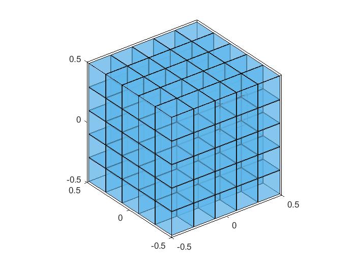
Figure 1: $125$ testcubes and $125$ Neumann patches.

Our simulations are based on noisy data. We assume that we are given a noise level $\eta\geq 0$ and set

$$\delta=\eta\cdot\|\bm{\Lambda}(\lambda,\mu)\|_{F}.$$

In addition, we define $\bm{\Lambda}^{\delta}(\lambda,\mu)$ as

$$\bm{\Lambda}^{\delta}(\lambda,\mu)=\bm{\Lambda}(\lambda,\mu)+\delta\overline{{\bf E}},$$

with $\overline{{\bf E}}={\bf E}/\|{\bf E}\|_{F}$, where ${\bf E}$ consists of $M\times M$ random uniformly distributed values in $[-1,1]$.

4.3.1 Example 1

For our simulations we calculate the maximal noise $\eta$ perturbing $\bm{\Lambda}(\lambda,\mu)$ for different background error parameters $\epsilon^{\lambda}$ and $\epsilon^{\mu}$ (see Figure 2), based on Theorem 3.

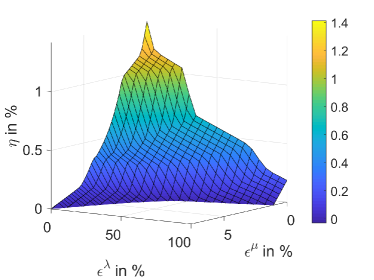
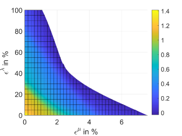
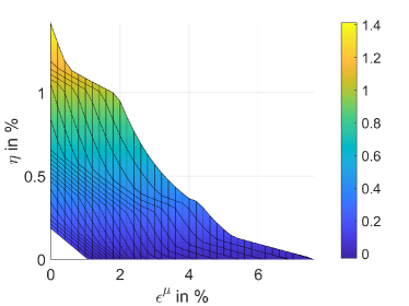
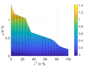
Figure 2: Relation between $\eta$ and $\epsilon^{\lambda}$ as well as $\epsilon^{\mu}$ for $125$ testcubes and $125$ Neumann patches shown from different angles.

Figure 2 tells us that the maximal $\eta$ of approximately $1.413\%$ is reached for $\epsilon^{\lambda}=0=\epsilon^{\mu}$. The background error $\epsilon^{\lambda}$ does not show much impact. Even for $\epsilon^{\lambda}=100\%$, we obtain a resolution guarantee. The maximal background error w.r.t. $\mu$ with $\epsilon^{\lambda}=0\%$ is $\epsilon^{\mu}\approx 7.692\%$ at $\eta=0\%$.

Remark 3.

All in all, we conclude that the resolution guarantees depend heavily on the Lamé parameter $\mu$ and only marginally on $\lambda$.

4.3.2 Example 2

Based on the result of Example 1, we change our configuration and set $\epsilon^{\lambda}=0\%$ for a better comparability. The results are shown in Figure 3-5, where we analyse the relation of $\epsilon^{\mu}$ ($x$-axis) and $\eta$ ($y$-axis) with both values given in $\%$. The considered numbers of testcubes and Neumann patches are given in the caption of the figure. As expected, the smaller the background error $\epsilon^{\mu}$ can be estimated, the more noise on the data can be handled.

In Figure 3, we deal with $5\times 5\times 5=125$ testcubes and $125$ Neumann patches as shown in Figure 1. We can observe an approximately linear connection between $\epsilon^{\mu}$ and $\eta$ showing that a resolution guarantee is given for all pairs $(\epsilon^{\mu},\eta)$ on the black line and the gray area below for $\epsilon^{\lambda}=0\%$.

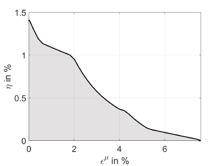
Figure 3: Relation between $\eta$ and $\epsilon^{\mu}$ for $125$ testcubes and $125$ Neumann patches for $\epsilon^{\lambda}=0\%$.

In Figure 4, we change our setting and increase the number of testcubes to $10\times 10\times 10=1000$, while simulating the reconstruction for the same $125$ Neumann patches.

If we now compare Figure 3 and 4, we see that for more testcubes, our method is less stable w.r.t. both $\epsilon^{\mu}$ and $\eta$. This behaviour is expected since smaller pixels are to be reconstructed with the same amount of data from the Neumann patches. Nevertheless, we achieve a resolution guarantee, if the pair $\eta$, $\epsilon^{\mu}$ is located on the black line or the gray area below. The maximal noise on the date is given by $\eta\approx 0.200\%$ for $\epsilon^{\mu}=\epsilon^{\lambda}=0\%$ and the maximal background noise for $\mu$ is given by $\epsilon^{\mu}\approx 0.927\%$ for $\epsilon^{\lambda}=\eta=0\%$.

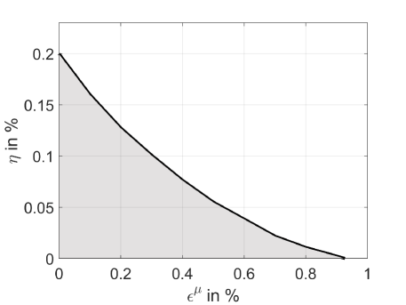
Figure 4: Relation between $\eta$ and $\epsilon^{\mu}$ for $1000$ testcubes and $125$ Neumann patches for $\epsilon^{\lambda}=0\%$.

Increasing the resolution by using more Neumann patches is also possible as indicated in Figure 5. This figure shows the set-up with $1000$ testcubes, the same as in Figure 4, but with $500$ Neumann patches instead of $125$. This increases both the stability regarding $\eta$ as well es $\epsilon^{\mu}$, however, the improvement is small. In fact, the maximal noise on the date is given by $\eta\approx 0.213\%$ for $\epsilon^{\mu}=\epsilon^{\lambda}=0\%$ and the maximal background noise for $\mu$ is given by $\epsilon^{\mu}\approx 0.942\%$ for $\epsilon^{\lambda}=\eta=0\%$. For a better resolution guarantee, even more Neumann patches have to be used, but the numerical effort to do that will increases heavily.

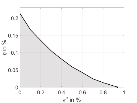
Figure 5: Relation between $\eta$ and $\epsilon^{\mu}$ for $1000$ testcubes and $500$ Neumann patches for $\epsilon^{\lambda}=0\%$.

5 Conclusion and outlook

Our main focus was the construction of conditions under which a resolution for a given partition can be achieved. Thus, our formulation takes both the background error as well as the measurement noise into account. The numerical simulations showed that for more testcubes our method is less stable w.r.t. $\epsilon^{\lambda},\epsilon^{\mu}$ and $\eta$. This behaviour is expected since more as well as smaller pixels are to be reconstructed with the same amount of data from the Neumann patches. As a main result, the resolution guarantees depend heavily on the Lamé parameter $\mu$ and only marginally on $\lambda$. Finally, we want to remark that the algorithm is more stable w.r.t. $\epsilon^{\lambda},\epsilon^{\mu}$ as w.r.t. $\eta$. All in all, our results are of special importance, when considering simulations based on real data, e.g., in [8] or in the framework of monotonicity-based regularization (see, e.g. [6]).

Acknowledgements
The first author thanks the German Research Foundation (DFG) for funding the project "Inclusion Reconstruction with Monotonicity-based Methods for the Elasto-oscillatory Wave Equation" (reference number $499303971$).

References

- [1] S Andrieux, AB Abda, and HD Bui. Reciprocity principle and crack identification. Inverse Problems, 15:59–65, 1999.
- [2] E Beretta, E Francini, A Morassi, E Rosset, and S Vessella. Lipschitz continuous dependence of piecewise constant Lamé coefficients from boundary data: the case of non-flat interfaces. Inverse Problems, 30(12):125005, 2014.
- [3] E Beretta, E Francini, and S Vessella. Uniqueness and Lipschitz stability for the identification of Lamé parameters from boundary measurements. Inverse Problems & Imaging, 8(3):611–644, 2014.
- [4] PG Ciarlet. The finite element method for elliptic problems. North Holland, 1978.
- [5] S Eberle and B Harrach. Shape reconstruction in linear elasticity: Standard and linearized monotonicity method. Inverse Problems, 37(4):045006, 2021.
- [6] S Eberle and B Harrach. Monotonicity-based regularization for shape reconstruction in linear elasticity. Comput. Mech., 2022.
- [7] S Eberle, B Harrach, H Meftahi, and T Rezgui. Lipschitz stability estimate and reconstruction of Lamé parameters in linear elasticity. Inverse Problems in Science and Engineering, 29(3):396–417, 2021.
- [8] S Eberle and J Moll. Experimental detection and shape reconstruction of inclusions in elastic bodies via a monotonicity method. Int J Solids Struct, 233:111169, 2021.
- [9] G Eskin and J Ralston. On the inverse boundary value problem for linear isotropic elasticity. Inverse Problems, 18(3):907, 2002.
- [10] R Ferrier, ML Kadri, and P Gosselet. Planar crack identification in 3D linear elasticity by the reciprocity gap method. Computer Methods in Applied Mechanics and Engineering, 355:193–215, 2019.
- [11] B Gebauer. Localized potentials in electrical impedance tomography. Inverse Probl. Imaging, 2(2):251–269, 2008.
- [12] B Harrach. On uniqueness in diffuse optical tomography. Inverse problems, 25(5):055010, 2009.
- [13] B Harrach. Simultaneous determination of the diffusion and absorption coefficient from boundary data. Inverse Probl. Imaging, 6(4):663–679, 2012.
- [14] B Harrach, YH Lin, and H Liu. On localizing and concentrating electromagnetic fields. SIAM J. Appl. Math, 78(5):2558–2574, 2018.
- [15] B Harrach and M Ullrich. Monotonicity-based shape reconstruction in electrical impedance tomography. SIAM Journal on Mathematical Analysis, 45(6):3382–3403, 2013.
- [16] B Harrach and M Ullrich. Resolution guarantees in electrical impedance tomography. IEEE Trans. Med. Imaging, 34(7):1513–1521, 2015.
- [17] S Hubmer, E Sherina, A Neubauer, and O Scherzer. Lamé parameter estimation from static displacement field measurements in the framework of nonlinear inverse problems. SIAM Journal on Imaging Sciences, 11(2):1268–1293, 2018.
- [18] M Ikehata. Inversion formulas for the linearized problem for an inverse boundary value problem in elastic prospection. SIAM Journal on Applied Mathematics, 50(6):1635–1644, 1990.
- [19] M Ikehata. Size estimation of inclusion. Journal of Inverse and Ill-Posed Problems, 6(2):127–140, 1998.
- [20] M Ikehata. Reconstruction of inclusion from boundary measurements. Journal of Inverse and Ill-posed Problems, 10(1):37–66, 2002.
- [21] M Ikehata. Stroh eigenvalues and identification of discontinuity in an anisotropic elastic material. Contemporary Mathematics, 408:231–247, 2006.
- [22] M Ikehata, G Nakamura, and K Tanuma. Identification of the shape of the inclusion in the anisotropic elastic body. Applicable Analysis, 72(1-2):17–26, 1999.
- [23] OY Imanuvilov and M Yamamoto. On reconstruction of Lamé coefficients from partial Cauchy data. Journal of Inverse and Ill-posed Problems, 19(6):881–891, 2011.
- [24] B Jadamba, AA Khan, and F Raciti. On the inverse problem of identifying Lamé coefficients inlinear elasticity. Computers and Mathematics with Applications, 56:431–443, 2008.
- [25] YH Lin and G Nakamura. Boundary determination of the Lamé moduli for the isotropic elasticity system. Inverse Problems, 33(12):125004, 2017.
- [26] L Marin and D Lesnic. Regularized boundary element solution for an inverse boundary value problem in linear elasticity. Communications in Numerical Methods in Engineering, 18:817–825, 2002.
- [27] L Marin and D Lesnic. Boundary element-Landweber method for the Cauchy problem in linear elasticity. IMA Journal of Applied Mathematics, 70(2):323–340, 2005.
- [28] G Nakamura, K Tanuma, and G Uhlmann. Layer stripping for a transversely isotropic elastic medium. SIAM Journal on Applied Mathematics, 59(5):1879–1891, 1999.
- [29] G Nakamura and G Uhlmann. Identification of Lamé parameters by boundary measurements. American Journal of Mathematics, pages 1161–1187, 1993.
- [30] G Nakamura and G Uhlmann. Inverse problems at the boundary for an elastic medium. SIAM journal on mathematical analysis, 26(2):263–279, 1995.
- [31] G Nakamura and G Uhlmann. Global uniqueness for an inverse boundary value problem arising in elasticity. Inventiones mathematicae, 152(1):205–207, 2003.
- [32] AA Oberai, NH Gokhale, MM Doyley, and JC Bamber. Evaluation of the adjoint equation based algorithm for elasticity imaging. Physics in Medicine and Biology, 49(13):2955–2974, 2004.
- [33] AA Oberai, NH Gokhale, and GR Feijoo. Solution of inverse problems in elasticity imaging using the adjoint method. Inverse Problems, 19:297–313, 2003.
- [34] DT Seidl, AA Oberai, and PE Barbone. The coupled adjoint-state equation in forward and inverse linear elasticity: Incompressible plane stress. Computer Methods in Applied Mechanics and Engineering, 357:112588, 2019.
- [35] P Steinhorst and AM Sändig. Reciprocity principle for the detection of planar cracks in anisotropic elastic material. Inverse Problems, 29:085010, 2012.
- [36] A Tamburrino. Monotonicity based imaging methods for elliptic and parabolic inverse problems. J. Inverse Ill-Posed Probl., 14(6):633–642, 2006.
- [37] A Tamburrino and G Rubinacci. A new non-iterative inversion method for electrical resistance tomography. Inverse Problems, 18(6):1809, 2002.