Nonequilibirum steady state for harmonically-confined active particles

Abstract

We study the full nonequilibirum steady state distribution $P_{\text{st}}\left(X\right)$ of the position $X$ of a damped particle confined in a harmonic trapping potential and experiencing active noise, whose correlation time $\tau_{c}$ is assumed to be very short. Typical fluctuations of $X$ are governed by a Boltzmann distribution with an effective temperature that is found by approximating the noise as white Gaussian thermal noise. However, large deviations of $X$ are described by a non-Boltzmann steady-state distribution. We find that, in the limit $\tau_{c}\to 0$, they display the scaling behavior $P_{\text{st}}\left(X\right)\sim e^{-s\left(X\right)/\tau_{c}}$, where $s\left(X\right)$ is the large-deviation function. We obtain an expression for $s\left(X\right)$ for a general active noise, and calculate it exactly for the particular case of telegraphic (dichotomous) noise.

I Introduction

I.1 Background

One of the fundamental problems in the study of non-equilibrium statistical mechanics and probability theory is fluctuations in stochastic systems. Rare events, or large deviations, are particularly interesting Varadhan ; O1989 ; DZ ; Hollander ; Bray ; Majumdar2007 ; hugo2009 ; Derrida11 ; RednerMeerson ; Vivo2015 ; MeersonAssaf2017 ; MS2017 ; Touchette2018 . Despite their small likelihood, they are of great interest because of their relevance to catastrophes like earthquakes, heatwaves, population extinction, and stock-market crashes. It is therefore important to develop theoretical frameworks that enable one to estimate their occurrence probability. Here, we study statistics of rare events within the context of active stochastic systems, which physically correspond to molecules and objects that consume energy from their environment and convert it into directed motion Mizuno07 ; Wilhelm08 ; Bruot11 ; Ahmed15 ; Breoni22 . Such systems are driven out of thermal equilibrium, and their dynamics may exhibit a multitude of counter-intuitive and rich phenomena Marchetti13 ; ALP14 ; FodorEtAl15 ; Kardar15 ; Dhar_2019 ; Fodor16 ; Needleman17 ; MalakarEtAl18 ; led19 ; WZKLT19 ; WKL20 ; led20 ; Basu20 ; SBS20 ; MB20 ; LMS21 ; ARYL21 ; WHB22 ; FJC22 ; SBS22 ; ARYL22 ; ACJ22 . In particular, they can relax to nonequilibrium steady states (NESSs), which in general cannot be described by a Boltzmann distribution.

The first-passage time (FPT) problem (or Kramers’ escape problem) is a classical problem in statistical mechanics RednerFPTBook ; BMS13 . In the simplest setting, one considers a particle that is trapped in a potential well and interacts with a noisy environment. The position $x$ of the particle at time $t$ is described by a Langevin equation, which for a system in one-dimension reads

$$m\ddot{x}+\Gamma\dot{x}+V^{\prime}\left(x\right)=\xi\left(t\right)\,,$$ (1)

where $m$ is the particle’s mass, $\Gamma>0$ is the damping coefficient, $V(x)$ is the external potential, and $\xi(t)$ is the noise. The FPT problem is that of determining the distribution of the first time $t_{\text{esc}}\left(X\right)$ at which $x(t)$ reaches some target $X$, given an initial condition. A related interesting quantity to study is the steady-state distribution (SSD), $P_{\text{st}}(X)$, of the position of the particle.

If $\xi(t)$ describes thermal noise, then it can be mathematically described by a white Gaussian noise with the following statistical properties: $\left\langle\xi\left(t\right)\right\rangle=0$, and, $\left\langle\xi\left(t\right)\xi\left(t^{\prime}\right)\right\rangle=2k_{B}T\Gamma\delta\left(t-t^{\prime}\right)$, where angular brackets denote the expectation value, and $k_{B}$ and $T$ denote Boltzmann’s constant and the temperature, respectively. For thermal noise, the SSD is given by the Boltzmann distribution,

$$P_{\text{st}}\left(X\right)\propto e^{-V\left(X\right)/k_{B}T}.$$ (2)

In the limit of low temperature and/or high barrier footnote:SM20 , the mean first passage time (MFPT) is approximately given by Kramers’ formula (the Arrhenius law) Kramers40 ; Hanggi90 ; Melnikov91

$$\left\langle t_{\text{esc}}\left(x=X\right)\right\rangle\sim e^{\Delta E/k_{B}T},$$ (3)

where $\Delta E$ is the difference between the potential energy at positions $X$ and at the minimum of the potential well, i.e., $\Delta E=V\left(X\right)-V_{\min}$.

A simple model of active particle dynamics is given by Eq. (1) with $\xi(t)$ that is not a thermal noise. In Refs. BenIsaac15 ; Wexler20 ; Woillez20 ; GP21 , a model was introduced and studied that is mathematically described by Eq. (1) with a harmonic trapping potential, $V\left(x\right)=kx^{2}/2$, and $\xi(t)$ that is the sum of a thermal noise and an active (non-thermal) noise with correlation time $\mathcal{T}_{c}$. The model was originally inspired by experiments in “active gels”, which consist of a network of actin filaments and myosin-II molecular motors in which the athermal nature of the random motion was probed by measuring the fluctuations of tracked tracer particles, and showing the fluctuation-dissipation theorem breaks down BHG06 ; Toyota11 ; Stuhrmann12 ; Mizuno07 . Position and velocity distributions and FPTs were studied BenIsaac15 ; Wexler20 ; Woillez20 , as well as the entropy production GP21 , but analytic progress could only be made in certain limiting cases, such as the limits of very large or very small $\mathcal{T}_{c}$. In the latter case, the MFPT was found to be given by Eq. (3), but with a modified, effective temperature $T_{\text{eff}}$, i.e., Wexler20

$$\left\langle t_{\text{esc}}\left(x=X\right)\right\rangle\sim e^{kX^{2}/2k_{B}T_{\text{eff}}}.$$ (4)

Here, we consider the case where $\xi(t)$ is a pure active noise (i.e., no thermal component footnote:thermalNoise ) in the limit $\mathcal{T}_{c}\to 0$ at a fixed noise amplitude. This case has to be distinguished from the case where simultaneously one also takes the noise amplitude to infinity with a proper scaling. In the latter, the correlation function of the noise becomes a delta function $\left\langle\xi\left(t\right)\xi\left(t^{\prime}\right)\right\rangle=2k_{B}T_{\text{eff}}\Gamma\delta\left(t-t^{\prime}\right)$, with some effective temperature $T_{\text{eff}}$, and Eq. (4) becomes exact colored . In the former, as we will show below, Eq. (4) (with $T_{\text{eff}}\propto\mathcal{T}_{c}$) faithfully describes the behavior of the system only for small $X$ which is sufficiently near the center of the trap. This result, however, breaks down at large $X$. One way to see this is to consider as an example noise terms that are bounded, e.g., a telegraphic active noise. For this kind of noise $x(t)$ is bounded too, leading to a divergence of the MFPT at some finite $X$, in contradiction with Eq. (3) (regardless of the definition of $T_{\text{eff}}$). This implies that, despite the timescale separation present in the system, detailed balance is violated. A similar situation was observed recently in a different context HG21 .

I.2 Precise definition of the problem, rescaling, and summary of main results

Let us consider the Langevin equation (1) in the particular case of a harmonic trapping potential $V\left(x\right)=kx^{2}/2$,

$$m\ddot{x}\left(t\right)+\Gamma\dot{x}\left(t\right)+kx\left(t\right)=\Sigma\left(t\right),$$ (5)

where $\Sigma\left(t\right)$ is telegraphic (dichotomous) noise, which switches between the values $\pm\Sigma_{0}$ at a constant rate $1/\mathcal{T}_{c}$, i.e., the time between every two consecutive switches is exponentially distributed with mean $\mathcal{T}_{c}$. Let us first rescale space and time, $kx/\Sigma_{0}\to x$, $\sqrt{k/m}\,t\to t$, so Eq. (5) becomes

$$\ddot{x}+\gamma\dot{x}+x=\sigma\left(t\right)\,,$$ (6)

where $\gamma=\Gamma/\sqrt{mk}$ and $\sigma\left(t\right)$ takes the values $\pm 1$, and the rescaled mean time for switching between these two values is $\tau_{c}=\sqrt{k/m}\,\mathcal{T}_{c}$. At long times, the system described by Eq. (6) will approach a steady state. Due to the active nature of the noise term, which violates detailed balance, this will be a nonequilibrium steady state. Our goal is to calculate the full SSD $P_{\text{st}}\left(X\right)$ of the particle’s position, including the tails of this distribution. Due to the mirror symmetry of the problem, $P_{\text{st}}\left(X\right)=P_{\text{st}}\left(-X\right)$ and the distributions of $t_{\text{esc}}\left(X\right)$ and $t_{\text{esc}}\left(-X\right)$ are identical, so we will only consider $X>0$ in what follows.

This problem, as formulated above, presents a significant theoretical challenge, and in order to make analytic progress, certain simplifying assumptions must be made. In the strongly-overdamped limit $\gamma\to\infty$, the SSD is known exactly for arbitrary trapping potentials $V(x)$ q-optics1 ; q-optics2 ; q-optics3 ; q-optics4 ; Kardar15 ; Dhar_2019 . In this work, we consider Eq. (6) with arbitrary damping coefficient $\gamma$, and focus on the limit of rapid switching rate of the noise term, $\tau_{c}\to 0$. In this limit, the rapid switching of the noise causes it to typically average out to zero over timescales that are relevant for the harmonic oscillator (which are of order unity in our choice of units). Hence, it becomes very unlikely to reach positions $X$ that are located away from the center of the trap, so that the SSD is strongly localized around $X=0$, and fluctuations become very rare. In order to study the full SSD (including its tails), it is thus natural to employ tools from large-deviation theory. In particular, we will combine the optimal-fluctuation method (OFM) (or weak-noise theory) Onsager ; MSR ; Freidlin ; Dykman ; Graham ; Falkovich01 ; GF ; EK04 ; Ikeda2015 ; Grafke15 ; bertini2015 ; Holcman ; SmithMeerson2019 ; MeersonSmith2019 ; AiryDistribution20 with the Donsker-Varadhan (DV) large-deviation formalism Bray ; Majumdar2007 ; hugo2009 ; TouchetteMinimalModel ; Touchette2018 ; Escamilla19 ; AiryDistribution20 in a novel way.

Let us summarize the principal results of this work. We find that, in the limit $\tau_{c}\to 0$, the SSD is given by

$$P_{\text{st}}\left(X\right)\sim e^{-s\left(X\right)/\tau_{c}}$$ (7)

where the large-deviation function (LDF) $s(X)$ does not depend on $\tau_{c}$. Thus, reaching any $X$ that is sufficiently far from the center of the trap is a large deviation. It then follows (see Appendix A) that the FPT to reach position $X$ follows an exponential distribution whose mean is given (in the limit $\tau_{c}\to 0$) by

$$\left\langle t_{\text{esc}}\left(X\right)\right\rangle\sim 1/P_{\text{st}}\left(X\right)\sim e^{s\left(X\right)/\tau_{c}}\,.$$ (8)

To be precise, we find a large-deviation principle (LDP)

$$-\lim_{\tau_{c}\to 0}\tau_{c}\ln P_{\text{st}}\left(X\right)=\lim_{\tau_{c}\to 0}\tau_{c}\ln\left\langle t_{\text{esc}}\left(X\right)\right\rangle=s\left(X\right)\,.$$ (9)

We calculate $s(X)$ exactly, by finding the optimal (most likely) trajectory of the particle, coarse-grained over timescales much longer than $\tau_{c}$, that starts at the center of the trap at time $t=-\infty$ and arrives at $x=X$ at time $t=0$. The LDF $s(X)$ displays a parabolic behavior around the center of the trap, at $X\ll 1$, matching the description in terms of a Boltzmann distribution with an effective temperature, as found in Wexler20 . We find intriguing qualitative differences between the system’s behavior between the overdamped ($\gamma>2$) and underdamped ($\gamma<2$) cases. In particular, we find that the SSD has a finite support $\left[-X_{0},X_{0}\right]$ (so the motion of the particle is bounded and it cannot leave this interval), where $X_{0}$ is a function of $\gamma$ that exhibits a transition at the critical value $\gamma=2$. Finally, we verify our theoretical predictions through extensive computer simulations, and discuss extensions to general trapping potentials and other types of active noise.

II Theoretical framework

Our theoretical framework consists of two main steps: (i) Providing an effective coarse-grained description of the dynamics that is valid over timescales much larger than $\tau_{c}$, which gives the probability of (coarse-grained) trajectories of the particle, (ii) Calculating the optimal history of the system that leads to a given $X$, i.e., the most likely (coarse-grained) trajectory $x(t)$ that satisfies the conditions $x(t\to-\infty)=0$ and $x(t=0)=X$. The first step relies on the well-established DV formalism, which we recall in Appendix B, while the second step involves the solution of a minimization problem from the calculus of variations, and essentially provides an extension of the OFM to active noise.

II.1 Coarse graining

In order to coarse grain the dynamics, let us consider the average of the noise term over a timescale $t$ that is much longer than $\tau_{c}$. We define

$$\bar{\sigma}=\frac{1}{t}\int_{0}^{t}\sigma\left(\tau\right)d\tau$$ (10)

Since the process $\sigma(t)$ is ergodic, its long-time averages converge to their corresponding ensemble-average values. Therefore, in the limit $t/\tau_{c}\to\infty$, $\bar{\sigma}\left(t\right)$ will approach its ensemble-average value which, for the telegraphic noise, is zero. Indeed, in the limit $\tau_{c}\to 0$ the noise effectively becomes very weak, making fluctuations of $\bar{\sigma}$ very unlikely. Nevertheless, one can quantify the probability for such fluctuations to occur. Fluctuations of integrals of stochastic processes (known as “dynamical” or additive observables) over long times have in fact been extensively studied, and there exists a well-established theoretical framework for studying them. This theory, sometimes referred to as Donsker-Varadhan (DV) theory, is based on a path-integral representation of the process and uses the Feynman-Kac formula Bray ; Majumdar2007 ; DonskerVaradhan ; Ellis ; hugo2009 ; Touchette2018 . The long-time behavior predicted by DV theory is that of an LDP for the probability density function (PDF) of the dynamical observable, describing an exponential decay in time. In our particular case, it predicts that the PDF $P\left(\bar{\sigma};t\right)$ of $\bar{\sigma}$ behaves as

$$P\left(\bar{\sigma};t\right)\sim e^{-t\Phi\left(\bar{\sigma}\right)/\tau_{c}},$$ (11)

where the rate function $\Phi\left(\bar{\sigma}\right)$ is independent of $t$ and $\tau_{c}$. Eq. (11) holds at fixed $\tau_{c}$, in the limit $t\to\infty$.

Importantly, by simply rescaling time, one finds that Eq. (11) holds at fixed $t$, in the limit $\tau_{c}\to 0$. The rate function $\Phi\left(z\right)$ that corresponds to telegraphic noise has been found in several contexts, such as run-and-tumble particles Dean21 and the Ehrenfest Urn model MeersonZilber18 , and it is given by

$$\Phi\left(z\right)=1-\sqrt{1-z^{2}}\,,$$ (12)

with $z$ confined to the interval $z\in\left[-1,1\right]$, as obviously must be the case since $\sigma(\tau)$ is itself bounded so that it cannot exceed this interval. A calculation of $\Phi\left(z\right)$, using DV theory, is given in Appendix B for completeness.

The coarse-graining procedure that we employ now is fairly standard but we will, nevertheless, explain it now in detail. We consider a sequence of time averages of the noise, $\bar{\sigma}_{1},\bar{\sigma}_{2},\dots,\bar{\sigma}_{N}$, defined as

$$\bar{\sigma}_{i}=\frac{1}{\Delta t_{i}}\int_{t_{i}}^{t_{i+1}}\sigma\left(\tau\right)d\tau\,,$$ (13)

for some sequence of $N$ time intervals, defined by $t_{\text{initial}}\equiv t_{1}<t_{2}<\dots<t_{N+1}\equiv t_{\text{final}}$, where $\Delta t_{i}=t_{i+1}-t_{i}$. In the limit $\tau_{c}\to 0$, the $\bar{\sigma}_{i}$’s become statistically independent, so their joint PDF $P\left(\bar{\sigma}_{1},\dots,\bar{\sigma}_{N}\right)$ is given by a product of their individual PDFs, each of which is given by Eq. (11), i.e.,

$$P\left(\bar{\sigma}_{1},\dots,\bar{\sigma}_{N}\right)\sim\exp\left[-\frac{1}{\tau_{c}}\sum_{i=1}^{N}\Delta t_{i}\Phi\left(\bar{\sigma}_{i}\right)\right]\,.$$ (14)

The final step in the coarse-graining procedure is to take the continuum limit in (14) by treating the index $i$ of $\bar{\sigma}_{i}$ as continuous. This requires a separation of timescales, between the short timescale $\tau_{c}$ and some longer characteristic timescale that depends on the physical system under study. We thus consider a coarse-grained noise $\bar{\sigma}\left(t\right)$ whose distribution is given by

$$P\left[\bar{\sigma}\left(t\right)\right]\sim e^{-s\left[\bar{\sigma}\left(t\right)\right]/\tau_{c}}\,,$$ (15)

$$s\left[\bar{\sigma}\left(t\right)\right]=\int_{t_{\text{initial}}}^{t_{\text{final}}}\Phi\left(\bar{\sigma}\left(t\right)\right)dt\,,$$ (16)

which is the continuum analog of (14). Eqs. (15) and (16) provide the basis for a coarse-grained, path-integral effective description of the telegraphic noise, which is valid at timescales much longer than $\tau_{c}$. It is worth noting that, since the rate function $\Phi$ is parabolic at small argument,

$$\Phi\left(z\right)\simeq z^{2}/2,\qquad|z|\ll 1,$$ (17)

it follows that at small noise amplitudes, $\left|\bar{\sigma}\right|\ll 1$, Eq. (16) reduces to the Wiener action

$$\frac{1}{2}\int_{t_{\text{initial}}}^{t_{\text{final}}}\bar{\sigma}\left(t\right)^{2}dt\,,$$

that describes white noise. However, signatures of the activity of the noise will become noticeable for $\bar{\sigma}\sim 1$.

We now return to our model given by Eq. (6). At fixed $\gamma$ and in the limit $\tau_{c}\to 0$, the characteristic timescales of the left hand side of the equation (describing a deterministic damped harmonic oscillator), which are of order unity, become much longer than $\tau_{c}$. Therefore, one can replace the telegraphic noise $\sigma\left(t\right)$ by its coarse-grained analog, i.e., one can consider the equation

$$\ddot{x}+\gamma\dot{x}+x=\bar{\sigma}\left(t\right)\,,$$ (18)

which, over timescales much larger than $\tau_{c}$, gives a correct effective description of the process defined by (6).

II.2 Optimal fluctuation method (OFM)

We now treat Eq. (18) as the starting point for an application of the OFM (which is sometimes referred to as “weak-noise theory”, or as “geometrical optics of diffusion” in the context of Brownian motion, and is also related to the “macroscopic fluctuation theory” of lattice gases). The OFM yields the (approximate) probability of the large deviation by finding the optimal (i.e., most likely) history of the system conditioned on the occurrence of the rare event Onsager ; MSR ; Freidlin ; Dykman ; Graham ; Falkovich01 ; GF ; EK04 ; Ikeda2015 ; Grafke15 ; bertini2015 ; Holcman ; SmithMeerson2019 ; MeersonSmith2019 ; AiryDistribution20 . This optimal history is in certain contexts referred to as an “instanton”.

At the heart of the OFM lies a saddle-point evaluation of the path integral representation of the process described by Eq. (18), which exploits the small parameter $\tau_{c}\ll 1$. The usual first step of the OFM would be to plug Eq. (18) into (15), in order to obtain an expression for the probability to observe some (coarse-grained) trajectory $x(t)$:

$$P\left[x\left(t\right)\right] \sim e^{-\tilde{s}\left[x\left(t\right)\right]/\tau_{c}}\,,$$ (19)

$$\tilde{s}\left[x\left(t\right)\right] = \int\Phi\left(\ddot{x}+\gamma\dot{x}+x\right)dt\,,$$ (20)

up to a Jacobian whose contribution is subleading in the limit $\tau_{c}\to 0$. This leads to a minimization problem for the action (20) over trajectories $x(t)$, which is to be solved subject to boundary conditions and/or constraints that depend on the particular problem that one is interested in solving. We are after the steady-state distribution $P_{\text{st}}\left(X\right)$, for which it is appropriate to consider trajectories $x(t)$ on the time interval $-\infty<t<0$, under the constraints

$$x\left(t\to-\infty\right) = 0\,,$$ (21)

$$x\left(t=0\right) = X\,.$$ (22)

Once the optimal trajectory – the minimizer of (20) under these constraints – is found, $P_{\text{st}}\left(X\right)$ is calculated by evaluating the action $s\left[x\left(t\right)\right]$ on the optimal trajectory, leading to the scaling behavior (7) reported above.

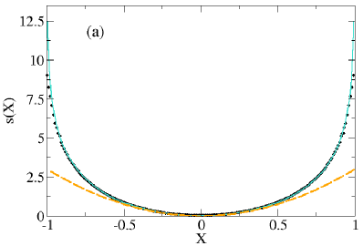
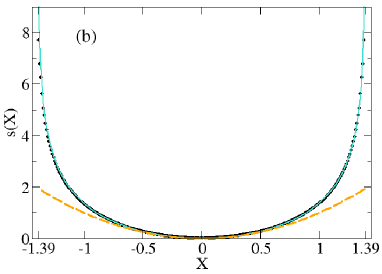
Figure 1: Solid curves: The LDFs $s(X)$ for $\gamma=3$ (a) and $\gamma=1$ (b), corresponding to the overdamped ($\gamma>2$) and underdamped ($\gamma<2$) cases, respectively. The most pronounced difference between the overdamped and underdamped regimes is the fact that $s(X)$ diverges at $\pm X_{0}$, where $X_{0}=1$ for $\gamma>2$ and $X_{0}>1$ for $\gamma<2$, see Fig. 4 below. Dashed curves: The approximation $s\left(X\ll 1\right)\simeq\gamma X^{2}$, corresponding to the description of the steady state through a Boltzmann distribution with an effective temperature. Symbols: Results of computer simulations.

However, the method outlined above leads to a technical difficulty in the present case, because the Euler-Lagrange equation associated with the functional (20) is a fourth-order nonlinear differential equation, due to the term with second derivative, $\ddot{x}$, in the functional. In order to bypass this difficulty, we use a shortcut which significantly simplifies the solution. The shortcut involves reformulating the problem as an optimization problem for the coarse-grained noise $\bar{\sigma}(t)$. The functional that is to be minimized,

$$s\left[\bar{\sigma}\left(t\right)\right]=\int_{-\infty}^{0}\Phi\left(\bar{\sigma}\left(t\right)\right)dt\,,$$ (23)

is a lot simpler because it contains no time derivatives. However, the constraint $x\left(t=0\right)=X$ takes a more complicated form in terms of $\bar{\sigma}$, which we now derive. Solving Eq. (18) for $x(t)$, we obtain

$$x\left(t\right)=\int_{-\infty}^{t}\bar{\sigma}\left(t^{\prime}\right)G\left(t,t^{\prime}\right)dt^{\prime}\,,$$ (24)

where

$$G\left(t,t^{\prime}\right)=\theta\left(t-t^{\prime}\right)\frac{e^{-a_{-}\left(t-t^{\prime}\right)}-e^{-a_{+}\left(t-t^{\prime}\right)}}{a_{+}-a_{-}}\,,$$ (25)

is the Green’s function for the forced damped harmonic oscillator, i.e., the solution of the equation

$$\partial_{t}^{2}G\left(t,t^{\prime}\right)+\gamma\partial_{t}G\left(t,t^{\prime}\right)+G\left(t,t^{\prime}\right)=\delta\left(t-t^{\prime}\right)$$ (26)

that satisfies $G\left(t,t^{\prime}\right)=0$ at $t<t^{\prime}$, and where

$$a_{\pm}=\frac{\gamma\pm\sqrt{\gamma^{2}-4}}{2}\,.$$ (27)

Using Eq. (24), the boundary condition $x\left(t=0\right)=X$ becomes

$$X=\int_{-\infty}^{0}\bar{\sigma}\left(t\right)G\left(0,t\right)dt=\int_{-\infty}^{0}\bar{\sigma}\left(t\right)\frac{e^{a_{-}t}-e^{a_{+}t}}{a_{+}-a_{-}}dt\,.$$ (28)

This reformulation of the problem as an optimization problem for $\bar{\sigma}$ makes its solution very easy. We take the constraint (28) into account via a Lagrange multiplier, i.e., we minimize the modified action

$$s_{\lambda}\left[\bar{\sigma}\left(t\right)\right]=s\left[\bar{\sigma}\left(t\right)\right]-\lambda X$$

$$\qquad=\int_{-\infty}^{0}\left[\Phi\left(\bar{\sigma}\left(t\right)\right)-\lambda\bar{\sigma}\left(t\right)\frac{e^{a_{-}t}-e^{a_{+}t}}{a_{+}-a_{-}}\right]dt\,.$$ (29)

The minimization becomes trivial because the functional does not contain any derivatives in time. One simply requires the derivative of the integrand in (II.2) with respect to $\bar{\sigma}\left(t\right)$ to vanish, yielding the optimal realization of the coarse-grained noise

$$\bar{\sigma}\left(t\right)=\left(\Phi^{\prime}\right)^{-1}\left(\lambda\frac{e^{a_{-}t}-e^{a_{+}t}}{a_{+}-a_{-}}\right)\,,$$ (30)

where

$$\left(\Phi^{\prime}\right)^{-1}\left(y\right)=\frac{y}{\sqrt{1+y^{2}}}$$ (31)

is the inverse function of $d\Phi/dz$ (where we recall that $\Phi$ is given in Eq. (12)).

In order to calculate the LDF $s(X)$, we first plug $\bar{\sigma}\left(t\right)$ from the solution (30) into Eq. (23), yielding $s$ as a function of $\lambda$:

$$s=\int_{-\infty}^{0}\Phi\left(\left(\Phi^{\prime}\right)^{-1}\left(\lambda\frac{e^{a_{-}t}-e^{a_{+}t}}{a_{+}-a_{-}}\right)\right)dt$$

$$=\int_{-\infty}^{0}\left(1-\frac{a_{+}-a_{-}}{\sqrt{\left(a_{+}-a_{-}\right)^{2}+\lambda^{2}\left(e^{a_{-}t}-e^{a_{+}t}\right)^{2}}}\right)dt\,.$$

The relation between $\lambda$ and $X$ is then found by plugging (30) into the constraint (28), yielding:

$$X=\int_{-\infty}^{0}\frac{e^{a_{-}t}-e^{a_{+}t}}{a_{+}-a_{-}}\left(\Phi^{\prime}\right)^{-1}\left(\lambda\frac{e^{a_{-}t}-e^{a_{+}t}}{a_{+}-a_{-}}\right)dt$$

$$=\!\int_{-\infty}^{0}\frac{\lambda\left(e^{a_{-}t}-e^{a_{+}t}\right)^{2}}{\left(a_{+}-a_{-}\right)\sqrt{\left(a_{+}-a_{-}\right)^{2}+\lambda^{2}\left(e^{a_{-}t}-e^{a_{+}t}\right)^{2}}}dt.$$

Eqs. (II.2) and (II.2) give the LDF $s(X)$ in a parametric form, and constitute the main theoretical result of this paper. This function $s(X)$ is plotted in the solid line in Fig. 1 for (a) $\gamma=3$ and (b) $\gamma=1$, corresponding to the overdamped and underdamped cases, respectively. The LDF $s(X)$ has a parabolic behavior around $X=0$ (displayed by the dashed curves in Fig. 1), and it diverges at $X=X_{0}$. The circle symbols denote the results of computer simulations which, indeed, show a very good agreement with the analytical predictions. The details of the computational methods are described in Appendix C.

Note that the dependence of our main results on the particular type of noise (which we took to be dichotomous) enters only through the rate function $\Phi(z)$. Therefore, for other types of active noise, the SSD can still be found, by first calculating the corresponding rate function $\Phi(z)$ and then plugging into the first lines of Eqs. (II.2) and (II.2) to obtain the LDF $s(X)$.

The OFM gives us additional useful information - the optimal (coarse-grained) realization of the process $x(t)$, conditioned on the constraint $x(0)=X$. This is now simply found by plugging Eq. (30) into (24):

$$x\left(t\right) = \int_{-\infty}^{t}\left(\Phi^{\prime}\right)^{-1}\left(\lambda\frac{e^{a_{-}t^{\prime}}-e^{a_{+}t^{\prime}}}{a_{+}-a_{-}}\right)$$ (34)

$$\times \frac{e^{-a_{-}\left(t-t^{\prime}\right)}-e^{-a_{+}\left(t-t^{\prime}\right)}}{a_{+}-a_{-}}dt^{\prime}\,.$$

Optimal paths are plotted in Fig. 2 for the overdamped and underdamped cases. These examples illustrate a general feature of the optimal trajectories: In the overdamped case $x$ is a monotonic function of $t$, whereas in the underdamped case $x$ oscillates with an amplitude that grows in time. This feature is not a consequence of the activity in the system, as it occurs also for the case of thermal noise, as will become immediately clear from the discussion of the case $X\ll 1$.

In the limit $X\ll 1$ (in which, as we will explain shortly in subsection II.3.1, the noise can be approximated as thermal, with no signature of activity in the leading order), the optimal trajectory becomes [using $\left(\Phi^{\prime}\right)^{-1}\left(y\ll 1\right)\simeq y$ in (34)]:

$$x\left(t\right)\simeq\frac{\lambda}{2\left(a_{+}-a_{-}\right)\left(a_{-}+a_{+}\right)}\left(\frac{e^{a_{-}t}}{a_{-}}-\frac{e^{a_{+}t}}{a_{+}}\right)\,.$$ (35)

This is nothing but the time-reversed relaxation trajectory for a particle that begins at position $X$ with zero velocity, and evolves in time in the absence of noise, i.e., according to $\ddot{x}+\gamma\dot{x}+x=0$. This is expected due to Onsager-Machlup symmetry for equilibrium systems Onsager , that follows from the time-reversal symmetry of the dynamics in the case of thermal noise.

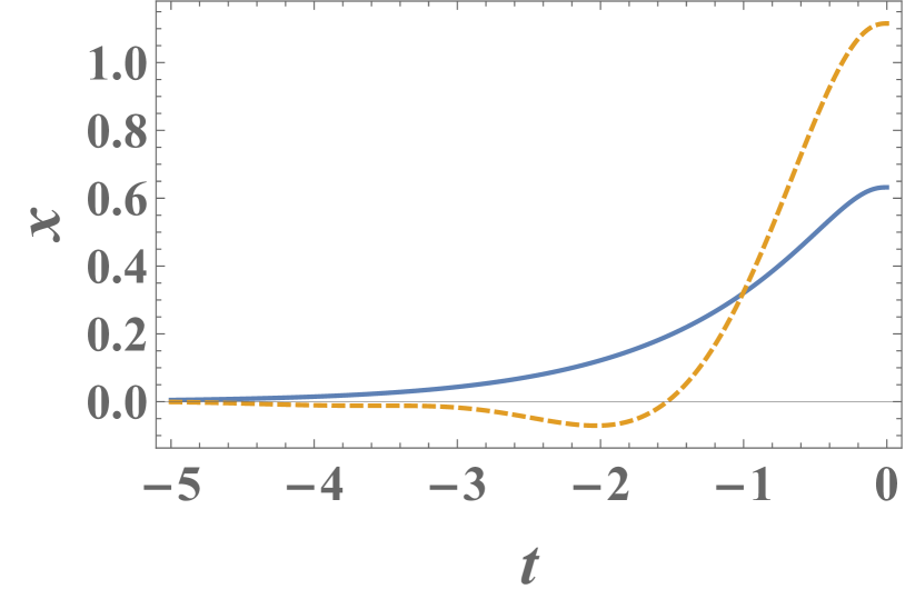
Figure 2: Optimal histories of the system $x(t)$ conditioned on reaching position $X$ at time $0$, see Eq. (34). Parameters are $\gamma=3$ and $\lambda=6$ for the overdamped case (solid line) and $\gamma=1$ and $\lambda=6$ for the underdamped case (dashed line), corresponding to $X=0.632168\dots$ and $X=1.1154\dots$, respectively.

II.3 Asymptotic limits

The results given above give the exact LDF, $s(X)$, at any $X$ and any $\gamma$. We now study the behavior of $s(X)$ in three limiting cases: Typical fluctuations $\left|X\right|\ll 1$, the behavior near the edge $X_{0}-\left|X\right|\ll X_{0}$, and the strongly-overdamped regime $\gamma\gg 1$.

II.3.1 Typical fluctuations $\left|X\right|\ll 1$

In the regime of typical fluctuations, $\left|X\right|\ll 1$, or equivalently $\left|\lambda\right|\ll 1$, Eqs. (II.2) and (II.2) simplify to

$$s\left(\lambda\ll 1\right)\simeq\frac{\lambda^{2}}{2\left(a_{+}-a_{-}\right)^{2}}\int_{-\infty}^{0}\left(e^{a_{-}t}-e^{a_{+}t}\right)^{2}dt=\frac{\lambda^{2}}{4\gamma}$$ (36)

and

$$X\left(\lambda\ll 1\right)\simeq\lambda\int_{-\infty}^{0}\frac{\left(e^{a_{-}t}-e^{a_{+}t}\right)^{2}}{\left(a_{+}-a_{-}\right)^{2}}dt=\frac{\lambda}{2\gamma}$$ (37)

respectively, so $s(X)$ is explicitly given by a parabola

$$s\left(X\ll 1\right)\simeq\gamma X^{2}\,.$$ (38)

Plugging Eq. (38) into (7), one finds that typical fluctuations follow a Gaussian distribution, which, in the physical variables, is given by

$$P_{\text{st}}\left(X\right)\sim e^{-\frac{\Gamma kX^{2}}{\mathcal{T}_{c}\Sigma_{0}^{2}}}\,.$$ (39)

We now show that Eq. (39) coincides with the result that one obtains by approximating the noise as white. The autocorrelation function of the noise is

$$\left\langle\Sigma\left(t\right)\Sigma\left(t^{\prime}\right)\right\rangle=\Sigma_{0}^{2}e^{-2\left|t-t^{\prime}\right|/\mathcal{T}_{c}}\,,$$ (40)

which satisfies

$$\int_{-\infty}^{\infty}\left\langle\Sigma\left(t\right)\Sigma\left(t^{\prime}\right)\right\rangle dt^{\prime}=\Sigma_{0}^{2}\mathcal{T}_{c}\,.$$ (41)

As discussed at the introduction, the telegraphic noise does not become white in the limit $\mathcal{T}_{c}\to 0$ at fixed $\Sigma_{0}$ footnote:whiteNoise . However, in the typical fluctuations regime $|X|\ll 1$, the white-noise approximation works well: The telegraphic noise can be approximated by an effective white (Gaussian) noise $\xi\left(t\right)$ with zero mean and correlation function $\left\langle\xi\left(t\right)\xi\left(t^{\prime}\right)\right\rangle=\Sigma_{0}^{2}\mathcal{T}_{c}\delta\left(t-t^{\prime}\right)$, which would physically describe a thermal noise with an effective temperature $T_{\text{eff}}=\Sigma_{0}^{2}\mathcal{T}_{c}/\left(2k_{B}\Gamma\right)$. This approximation yields a Boltzmann steady-state distribution,

$$P_{\text{st}}\left(X\right)\sim e^{-\frac{V\left(X\right)}{k_{B}T_{\text{eff}}}},$$ (42)

which, after plugging in the value of $T_{\text{eff}}$ as well as $V_{k}\left(x\right)=kx^{2}/2$, indeed coincides with (39).

Eq. (38) can be seen to correctly describe the small-$|X|$ behavior of the exact $s(X)$ in Fig. 1 for $\gamma=1$ and $\gamma=3$. As is seen in the figure, $s(X)$ lies above its parabolic approximation (38), leading to probabilities $P_{\text{st}}\left(X\right)$ that are smaller. Physically, this means that the boundedness of the noise makes it less likely to reach large $X$’s, when compared to the white-noise case. This effect is very small at small $X$, and becomes more important as $X$ is increased, while at $X>X_{0}$ it dominates and leads to $P_{\text{st}}\left(X\right)=0$.

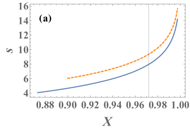
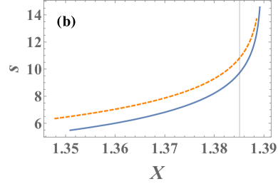
Figure 3: Solid lines: The LDF $s(X)$ for $\gamma=3$ (a) and $\gamma=1$ (b), as in Fig. 1, at $X\simeq X_{0}$. Dashed lines: the approximations near the edges, given by Eqs. (47) and (55), respectively. In (b), $X_{0}=\coth\left(\frac{\pi}{2\sqrt{3}}\right)=1.38958\dots$.

II.3.2 Near the edges of the support, $X_{0}-\left|X\right|\ll X_{0}$

Let us now study the opposite limit, in which the particle is very close to the edges, $X_{0}-X\ll X_{0}$, which corresponds to $\lambda\to\infty$. In order to do so, we first analyze the behavior of $\bar{\sigma}\left(t\right)$ from Eq. (30), at $\lambda\gg 1$. We consider first the overdamped case, $\gamma>2$. At sufficiently early times, the exponential terms are negligible, so $\bar{\sigma}\left(t\right)$ vanishes in the leading order. From time

$$t_{\lambda}=\frac{1}{a_{-}}\ln\left(\frac{a_{+}-a_{-}}{\lambda}\right)$$ (43)

onwards, the term $\lambda e^{a_{-}t}$ becomes very large and dominates. As a result, using $\left(\Phi^{\prime}\right)^{-1}\left(y\gg 1\right)\simeq 1$ we find $\bar{\sigma}\left(t\right)\simeq 1$. Finally, very close to $t=0$, one has $e^{a_{-}t}-e^{a_{+}t}\simeq 0$ ultimately leading to $\bar{\sigma}\left(t=0\right)=0$. To summarize,

$$\bar{\sigma}\left(t\right)\simeq\begin{cases}0,&t<t_{\lambda}\text{ or }t\simeq 0,\\[2.84526pt] 1,&t_{\lambda}<t<0.\end{cases}$$ (44)

We verified the validity of the approximation (44) in Appendix E.

The action is very easy to calculate in this limit. From Eq. (23), one simply obtains

$$s\left(\lambda\gg 1\right)\simeq-t_{\lambda}\simeq\frac{\ln\lambda}{a_{-}}\,,$$ (45)

where we neglected the term $a_{+}-a_{-}$ in (43) in order to avoid excess of accuracy. The relation between $X$ and $\lambda$ also simplifies in this limit. Plugging Eq. (44) into (28) (replacing $\bar{\sigma}\to P$,) we obtain

$$X\simeq\int_{t_{\lambda}}^{0}\frac{e^{a_{-}t}-e^{a_{+}t}}{a_{+}-a_{-}}dt\simeq 1-\frac{1}{a_{-}\lambda}\,.$$ (46)

This result, in particular, implies that $X_{0}=1$ for the overdamped case, corresponding to the particle’s mechanical equilibria for the situation in which the noise is $\sigma=1$. Putting Eqs. (45) and (46) together, we obtain the asymptotic behavior

$$s\left(X\right)\simeq-\frac{1}{a_{-}}\ln\left(1-X\right),\quad 1-X\ll 1\,,$$ (47)

see Fig. 3 (a). The physical picture in this limit is quite simple: The noise $\bar{\sigma}\left(t\right)$ acts as a constant force, pushing the particle towards the position $X$, for duration $\left|t_{\lambda}\right|$.

Let us now consider the underdamped case, $\gamma<2$. In this case, Eq. (30) takes the form

$$\bar{\sigma}\left(t\right)=\left(\Phi^{\prime}\right)^{-1}\left(-\frac{2\lambda}{\sqrt{4-\gamma^{2}}}e^{\gamma t/2}\sin\left(\frac{\sqrt{4-\gamma^{2}}}{2}t\right)\right)\,.$$ (48)

Eq. (48) is exact. Let us now analyze its behavior in the limit $\lambda\gg 1$. At sufficiently early times, the exponential decay again leads to $\bar{\sigma}\left(t\right)\simeq 0$. From time $t_{\lambda}=-2\left(\ln\lambda\right)/\gamma$ onwards, the exponential term becomes very large. As a result, the argument of $\left(\Phi^{\prime}\right)^{-1}$ becomes much larger than 1 in absolute value, except for short temporal boundary layers in which the term with $\sin$ vanishes, signaling a sign change of $\bar{\sigma}\left(t\right)$. Using

$$\left(\Phi^{\prime}\right)^{-1}\left(y\right)\simeq\text{sgn}\left(y\right),\qquad\left|y\right|\gg 1,$$ (49)

we thus obtain

$$\bar{\sigma}\left(t\right)\simeq\begin{cases}0,&t<t_{\lambda},\\[5.69054pt] -\text{sgn}\left(\sin\left(\frac{\sqrt{4-\gamma^{2}}}{2}t\right)\right),&t_{\lambda}<t<0\end{cases}$$ (50)

(see Appendix E for a check of this approximation). This leads, using Eq. (23), to

$$s\left(\lambda\gg 1\right)\simeq-t_{\lambda}=\frac{2\ln\lambda}{\gamma}\,.$$ (51)

One way to find the connection between $X$ and $\lambda$ is to analyze the expression (II.2) in the limit $\lambda\gg 1$. However, this turns out to be rather difficult from a technical point of view. Instead, we will employ a useful shortcut that bypasses this calculation. The shortcut makes use of the relation $ds/dX=\lambda$, a property that follows from the fact that $X$ and $\lambda$ are conjugate variables, see e.g. Ref. Vivoetal . Using this property together with the chain rule, we obtain

$$\frac{ds}{d\lambda}=\frac{ds}{dX}\frac{dX}{d\lambda}=\lambda\frac{dX}{d\lambda}\,.$$ (52)

Using Eq. (51), we find

$$\frac{dX}{d\lambda}=\frac{1}{\lambda}\frac{ds}{d\lambda}\simeq\frac{2}{\gamma\lambda^{2}}\,,$$ (53)

which we immediately integrate to obtain

$$X\simeq X_{0}-\frac{2}{\gamma\lambda}\,,$$ (54)

where the integration constant $X_{0}$ will be determined shortly. Putting these results together, we obtain the asymptotic behavior

$$s\left(X\right)\simeq-\frac{2}{\gamma}\ln\left(X_{0}-X\right),\qquad X_{0}-X\ll X_{0}\,,$$ (55)

see Fig. 3 (b).

Let us now calculate $X_{0}$. Plugging Eq. (50) into (28), we obtain

$$X = -\frac{2}{\sqrt{4-\gamma^{2}}}\int_{-\infty}^{0}\bar{\sigma}\left(t\right)e^{\gamma t/2}\sin\left(\frac{\sqrt{4-\gamma^{2}}}{2}t\right)dt\simeq$$ (56)

$$\simeq \frac{2}{\sqrt{4-\gamma^{2}}}\int_{t_{\lambda}}^{0}e^{\gamma t/2}\left|\sin\left(\frac{\sqrt{4-\gamma^{2}}}{2}t\right)\right|dt\,.$$

In order to calculate $X_{0}$ as a function of $\gamma$, we simply take the limit $\lambda\to\infty$, in which one has $t_{\lambda}\to-\infty$, so

$$X_{0} = \frac{2}{\sqrt{4-\gamma^{2}}}\int_{-\infty}^{0}e^{\gamma t/2}\left|\sin\left(\frac{\sqrt{4-\gamma^{2}}}{2}t\right)\right|dt$$ (57)

$$= \coth\left(\frac{\pi\gamma}{2\sqrt{4-\gamma^{2}}}\right)\,.$$

The details of the solution of the integral in Eq. (57) are given in Appendix D. In Fig. 4, $X_{0}$ is plotted as a function of $\gamma$. The particle cannot reach the region $X>X_{0}$, i.e., $P_{\text{st}}\left(X\right)$ vanishes there. The divergence of the LDF at $X\to X_{0}$, as given by Eqs. (47) and (55), describes the manner in which $P_{\text{st}}\left(X\right)$ vanishes as $X\to X_{0}$.

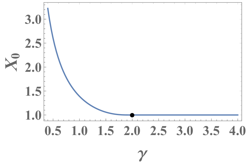
Figure 4: The maximal possible position of the particle, $X_{0}$, as a function of the damping coefficient $\gamma$, which is given by Eq. (57) in the underdamped case $\gamma<2$ and by $X_{0}=1$ for $\gamma>2$.

II.3.3 Strongly-overdamped regime $\gamma\gg 1$

Here we study the strongly-overdamped regime, $\gamma\gg 1$, or $m\to 0$ in the physical variables. In this limit, the motion described by Eq. (5) can be interpreted as that of a run-and-tumble particle confined in a harmonic potential Kardar15 ; Maes2018 ; Dhar_2019 ; Basu20 . As we mentioned in the Introduction, in this limit the SSD is known exactly for telegraphic noise with any trapping potential $V(x)$ VBH84 ; q-optics1 ; q-optics2 ; q-optics3 ; q-optics4 ; colored ; Kardar15 ; Dhar_2019 ; Basu20 . Up to a normalization factor, the SSD is given, in the physical variables, by

$$P_{\text{st}}\left(X\right)\propto\frac{\Gamma^{2}}{\Sigma_{0}^{2}-F^{2}(X)}\exp\left[\frac{2\Gamma}{\mathcal{T}_{c}}\int_{0}^{X}dy\frac{F(y)}{\Sigma_{0}^{2}-F^{2}(y)}\right]\,,$$ (58)

where $F\left(x\right)=-V^{\prime}\left(x\right)$ is the force that acts on the particle. In the case of the harmonic potential $V(x)=kx^{2}/2$, this becomes Dhar_2019 ; TC08

$$P_{\text{st}}\left(X\right)\propto\exp\left[\left(\frac{\Gamma}{k\mathcal{T}_{c}}-1\right)\ln\left(\Sigma_{0}^{2}-k^{2}X^{2}\right)\right]\,.$$ (59)

In the limit $\mathcal{T}_{c}\to 0$, the term ‘$-1$’ in the exponential in Eq. (59) is negligible compared to the term $\Gamma/k\mathcal{T}_{c}$, and one recovers our Eq. (7) with the LDF

$$s(X)=-\gamma\ln\left(1-X^{2}\right)$$ (60)

(in the rescaled variables).

Figure 5: Solid line: The exact LDF $s(X)$ for $\gamma=4$. This value of $\gamma$ turns out to be sufficiently large for the strongly-overdamped approximation (60) (dashed line) to work very well, as is clearly seen in the figure.

Let us show that the LDF given by Eqs. (II.2) and (II.2) indeed recovers this result when $\gamma\gg 1$. In this limit, Eq. (27) becomes

$$a_{+}\simeq\gamma,\qquad a_{-}\simeq\frac{1}{\gamma}\,,$$ (61)

so $a_{+}\gg a_{-}$. As a result, the two exponential terms in Eq. (II.2) decay over very different timescales, so we can safely discard the faster-decaying one, leading to

$$s\simeq\int_{-\infty}^{0}\left(1-\frac{\gamma}{\sqrt{\gamma^{2}+\lambda^{2}e^{2t/\gamma}}}\right)dt\,.$$ (62)

In Appendix F we solve this integral, and then use the shortcut (52) yielding explicit expressions for $s$ and $X$ as functions of $\lambda$, from which we indeed recover Eq. (60). In Fig. 5, the exact $s(X)$ is plotted together with the approximation (60) for $\gamma=4$. The two plots are indistinguishable within the scale of the figure.

III Conclusion

In this paper, we calculated the SSD (and from it, the MFPT) of a damped particle which experiences an external harmonic force, and is driven by telegraphic (dichotomous) noise, in the limit where the switching rate of the noise is very large. In the typical-fluctuations regime, the noise can be approximated as white, leading to a Boltzmann distribution for the SSD and an Arrhenius law for the MFPT, with an effective temperature that is easy to calculate from the correlation function of the noise. However, in the large-deviations regime, the effective thermal description of the system breaks down. We found that both the SSD and the MFPT follow large-deviation principles, Eqs. (7) and (8) respectively. We proceeded to calculate the large-deviation function $s(X)$ analytically, see Eqs. (II.2) and (II.2), showing very good agreement with Langevin Dynamics simulations (see also Appendix C).

We found that, at a coarse-grained temporal scale, the dominant contribution to the probability for observing the particle at some position $X$ comes from an optimal trajectory $x(t)$ [and a corresponding optimal coarse-grained noise realization $\bar{\sigma}\left(t\right)$]. We observed a qualitative difference in the behavior between the overdamped and underdamped regimes: In the former, the noise $\bar{\sigma}\left(t\right)$ pushes $x(t)$ monotonically towards $X$, whereas in the latter, $x(t)$ oscillates with a growing amplitude, while $\bar{\sigma}\left(t\right)$ changes sign every half-oscillation, increasing the particle’s energy until it reaches $X$. In both cases, the particle is confined in space $x\left(t\right)<X_{0}$, with $X_{0}=1$ in the overdamped case, but $X_{0}>1$ in the underdamped case, see Eq. (57). Notably, our coarse-graining procedure maintains the nonequlibrium (active) character of the noise, cf. HG21 .

It is worth mentioning the recent work AgranovBunin21 , in which the stochastic dynamics of two populations was studied, and a separation of timescales was exploited in order to employ a ‘hybrid’ DV-OFM approach that is similar in spirit to ours. In the current work we point out that this method can be applied quite generally, and demonstrate that it is especially useful in systems with non-Gaussian noise with a short correlation time.

Our main result for $s(X)$ can be straightforwardly extended to other types of active noise whose associated rate function $\Phi(z)$ can be found, by simply plugging $\Phi(z)$ into the first lines of Eqs. (II.2) and (II.2). A second immediate extension is to a noise term $\xi(t)$ in Eq. (1) (with a harmonic potential) that is given by the sum of two (or more) statistically-independent noises, e.g., the sum of active and thermal noises BenIsaac15 ; Wexler20 ; Woillez20 ; GP21 ; Tucci22 . Due to the linearity of the equation, one finds that the SSD is given (exactly) by the convolution of the SSDs that correspond to each of the two noise terms separately Tucci22 ; Frydel22 ; SLMS22 . Finally, it would be interesting to extend our results to anharmonic potentials Wexler20 ; led20 higher spatial dimensions ABP2018 ; Malakar20 ; Basu20 ; SBS20 ; MB20 ; SBS21 ; Frydel22 ; SBS22 ; SLMS22 , and to interacting run-and-tumble particles LMS21 .

Acknowledgments

NRS acknowledges helpful discussions with Golan Bel, Tal Agranov and Baruch Meerson and is grateful to Pierre Le Doussal, Satya Majumdar and Grégory Schehr for a collaboration on related topics. We are grateful to Yariv Kafri for a helpful correspondence and for pointing out several references.

Appendix A Relation between the FPT distribution and the SSD

To reach the relation

$$\left\langle t_{\text{esc}}\left(X\right)\right\rangle\sim 1/P_{\text{st}}\left(X\right)$$ (63)

between the MFPT and the SSD that is given in Eq. (8) of the main text, one partitions the dynamics into intervals whose duration is several times longer than the system’s correlation time (which is unity in our rescaled units). Then the intervals are approximately statistically independent, and the probability of reaching the target $X$ in each of the intervals is proportional to $P_{\text{st}}\left(X\right)$, which is assumed to be very small. Thus the FPT to reach the target $X$ obeys an exponential distribution whose mean is given by Eq. (63), as stated in the main text. Relations such as (63) between MFPTs and SSDs (or quasi-SSDs) occur in many situations when considering large deviations in stochastic dynamical systems, see for instance Refs. WZKLT19 ; WKL20 in the context of active matter, and MeersonAssaf2017 in the context of stochastic population dynamics. An even simpler example comes from the Arrhenius law (3) and Boltzmann distribution (2).

Appendix B Donsker-Varadhan formalism

Here, for completeness, we briefly outline the Donsker-Varadhan (DV) formalism DonskerVaradhan , and apply it to the telegraphic noise in order to calculate the rate function $\Phi(z)$ that is given in Eq. (12) of the main text. For an accessible introduction and further details regarding the general DV theory, we refer the reader to Ref. Touchette2018 . Let $y\left(t\right)$ be a stochastic process with a finite state space, $y\left(t\right)\in\left\{y_{1},\dots,y_{n}\right\}$, and let

$$\frac{d\mathbold{v}}{dt}=L\mathbold{v}$$ (64)

be the master equation that describes the temporal evolution of the probability vector $\mathbold{v}=\left(v_{1},\dots,v_{n}\right)$, where $v_{i}(t)$ denotes the probability that $y\left(t\right)=y_{i}$. Here $L$, the generator of the dynamics, is an $n\times n$ matrix. Define a dynamical observable

$$A=\frac{1}{T}\int_{0}^{T}y\left(t\right)dt\,,$$ (65)

and consider its PDF $p_{T}\left(a\right)$, defined via

$$\text{Prob}\left(A\in\left[a,a+da\right]\right)=p_{T}\left(a\right)da$$ (66)

for infinitesimal $da$. Then the DV formalism predicts that, in the limit $T\to\infty$, an LDP holds:

$$p_{T}\left(a\right)\sim e^{-TI\left(a\right)}\,.$$ (67)

Moreover, it provides a method of calculating the rate function $I(a)$, by making use of the Gärtner-Ellis theorem Ellis . From this theorem it follows that $I(a)$ is the Legendre-Fenchel transform

$$I\left(a\right)=\max_{k\in\mathbb{R}}\left[ka-\mu\left(k\right)\right]$$ (68)

of the scaled cumulant generating function (SCGF)

$$\mu\left(k\right)=\lim_{T\to\infty}\frac{1}{T}\left\langle e^{TkA}\right\rangle\,.$$ (69)

Finally, the SCGF is given by the maximum eigenvalue of an auxiliary matrix operator

$$L_{i,j}^{k}=\left(L^{\dagger}\right)_{i,j}+ky_{i}\delta_{i,j}\,,$$ (70)

which is a “tilted” version of the Hermitian conjugate of $L$. Here $\delta_{i,j}$ is the Kronecker delta.

Let us apply this formalism to the (rescaled) telegraphic noise $\sigma(t)$ that is defined in the main text. Its two possible states are $\sigma\left(t\right)\in\left\{1,-1\right\}$, and the generator of the dynamics of $\sigma(t)$ is the matrix

$$L=\frac{1}{\tau_{c}}\left(\begin{array}[]{cc}-1&1\\ 1&-1\end{array}\right)\,.$$ (71)

Therefore, the SCGF is given by the largest eigenvalue of the matrix

$$L^{k}=\frac{1}{\tau_{c}}\left(\begin{array}[]{cc}-1&1\\ 1&-1\end{array}\right)+k\left(\begin{array}[]{cc}1&0\\ 0&-1\end{array}\right)\,.$$ (72)

The largest eigenvalue of $L^{k}$ is

$$\mu\left(k\right)=\sqrt{k^{2}+\frac{1}{\tau_{c}^{2}}}\,-\frac{1}{\tau_{c}}\,.$$ (73)

Since this function is convex, the Legendre-Fenchel transform becomes a Legendre transform, and we obtain

$$I\left(a\right)=\frac{1-\sqrt{1-a^{2}}}{\tau_{c}}\,,$$ (74)

recovering Eq. (12) of the main text.

Appendix C Langevin Dynamics simulations

In order to verify the accuracy of Eqs. (II.2) and (II.2), which constitute the analytical expression for the LDF $s(X)$, we need to compute $P_{\rm st}(X)$, and then to extract $s(X)$ from Eq. (7) [or practically, from the logarithmic version of it, Eq. (9)]. The SSD can be obtained by simulating an ensemble of long trajectories of particles that follow the Langevin equation of motion (6), where for each trajectory an independent realization of the telegraphic noise $\sigma(t)$ with a characteristic switching time $\tau_{c}$ is randomly chosen. The duration of the simulated trajectories $t$ must be sufficiently large to ensure that steady state is established, while $\tau_{c}$ must be sufficiently small in order to approach the limit $\tau_{c}\rightarrow 0$ of interest. Strictly speaking, in this straightforward approach, the computed $P_{\rm st}(X)$ is expected to converge to the correct SSD when the number of simulated trajectories becomes infinitely large. In practice, however, this strategy fails in the large deviation regime $X\lesssim X_{0}$ (which is of most interest) because of the remarkably low probability of a trajectory to actually reach near the edges of the support. To better appreciate the difficulty to sample the large deviation regime, consider the case $\gamma=3$ [see Fig. 1 (a)]. The first problem that we encounter is the lack of a priori knowledge which $\tau_{c}$ is “sufficiently close to zero”. A reasonable choice may be $\tau_{c}=0.2$, which is smaller than the other (rescaled) time constants relevant to the dynamics, i.e., (i) the inverse oscillator frequency $\sqrt{k/m}=1$ and (ii) the friction damping time $m/\Gamma=1/\gamma=1/3$. However, for this value of $\tau_{c}$, the probability to be in the range $|X|>0.95$ [$s(X=0.95)\simeq 6.5$] is smaller than $10^{-15}$, and the probability to reach $|X|>0.98$ [$s(X=0.98)\simeq 9$] is smaller than $10^{-21}$. These numbers suggest that proper sampling of the large deviation regime may require simulations of a prohibitively large number of trajectories. Furthermore, even if we had the resources to do so, we would still not know the difference between the LDF computed for a small finite $\tau_{c}$ and the one expected in the limit $\tau_{c}\rightarrow 0$.

Generally speaking, the number of times that the direction of the noise changes in large deviations trajectories is considerably smaller than the most probable number of switches, $n^{*}=t/\tau_{c}$, which is characteristic of typical trajectories. In order to properly sample such rare trajectories, we use the exact relationship

$$P(X)=\sum_{n=0}^{\infty}P(X|n)\Pi_{n},$$ (75)

where $P(X|n)$ is the conditional probability that the trajectory ended at $x=X$ given that noise underwent $n$ switches during the course of the motion, and $\Pi_{n}$ is the probability that the noise changed sign exactly $n$ times. The latter is given by the Poisson distribution

$$\Pi_{n}=\frac{e^{-t/\tau_{c}}}{n!}\left(\frac{t}{\tau_{c}}\right)^{n}.$$ (76)

A trajectory with $n$ switching points consists of $n+1$ segments during which the particle experiences a constant noise of magnitude $\pm 1$. In order to generate such a trajectory, we draw $n+1$ random numbers $R_{i}$ from a standard exponential distribution, and then rescale them $R_{i}\rightarrow R_{i}(t/\sum_{j=1}^{n+1}R_{j})$ to obtain the durations of the dynamical segments. For a harmonic confining potential, the equation of motion along each segment can be easily solved, which yields the position and velocity of the particle at each switching point. Once the trajectory has reached completion, the position of the particle is recorded, and by simulating many trajectories with $n$ switches, we obtain $P(X|n)$. An important merit of this approach (besides the simulations of many rare trajectories) is the fact that with the data for $P(X|n)$ (which depends on $t$ but not on $\tau_{c}$), we can use Eq. (76) to calculate the SSD for any $\tau_{c}$ provided that the largest simulated $n$ is somewhat larger than $n^{*}=t/\tau_{c}$. We can, thus, compute $s(X)$ for several values of $\tau_{c}$, and then extrapolate the results to the limit $\tau_{c}\rightarrow 0$.

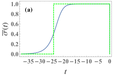
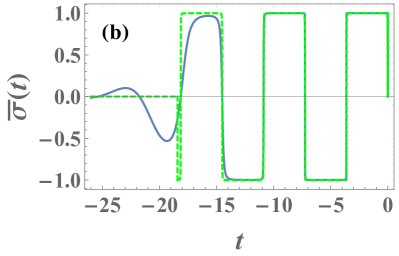
Figure 6: The optimal realization $\bar{\sigma}\left(t\right)$ of the coarse-grained noise term, $\bar{\sigma}(t)$, in the limit $\lambda\gg 1$, in the overdamped (a) and underdamped (b) cases. Solid lines correspond to the exact result (30). Dashed lines correspond to the approximate expressions, (44) and (50) respectively. Parameters are $\gamma=3$ and $\lambda=10^{4}$, corresponding to $X=0.999738\dots$ in (a), and $\gamma=1$ and $\lambda=10^{4}$, corresponding to $X=1.38938\dots$ in (b). Recall that in (a) the edge of the support of the SSD is at $X_{0}=1$ while in (b), it is at $X_{0}=\coth\left(\frac{\pi}{2\sqrt{3}}\right)=1.38958\dots$.

The results presented in Fig. 1 are based on simulations of $10^{9}$ trajectories of duration $t=10$, for values of $n$ in the range $0\leq n\leq 275$. The displayed $s(X)$ is an extrapolation of the LDFs calculated for $\tau_{c}=0.2$, 0.3, 0.4, and 0.5. For $\gamma=3$, the computational data is indistinguishable from the analytical predictions at $|X|<0.92$, and at $0.92<|X|<0.96$ the difference is at most 5%. We note that: (i) Simulating straightforwardly (with an overall similar CPU time) the dynamics with $\tau_{c}=0.2$ yielded no single trajectory with $|X|>0.87$. (ii) In a future publication we will demonstrate how the approach presented herein can be further improved.

Appendix D Solving the integral for $X_{0}$ in the underdamped regime

In this appendix we solve the integral that appears in the first line of Eq. (57) of the main text, thereby obtaining the second line in that equation. Denoting $\omega\equiv\sqrt{4-\gamma^{2}}\,/2$, the first line of Eq. (57) can be rewritten as $X_{0}=I/\omega$ where

$$I=\int_{-\infty}^{0}e^{\gamma t/2}\left|\sin\left(\omega t\right)\right|dt\,.$$ (77)

We now divide the integration region into two parts, and obtain

$$I=\int_{-\infty}^{-\pi/\omega}e^{\gamma t/2}\left|\sin\left(\omega t\right)\right|dt+\int_{-\pi/\omega}^{0}e^{\gamma t/2}\left|\sin\left(\omega t\right)\right|dt$$

$$=e^{-\pi\gamma/2\omega}\int_{-\infty}^{0}e^{\gamma t/2}\left|\sin\left(\omega t\right)\right|dt-\int_{-\pi/\omega}^{0}e^{\gamma t/2}\sin\left(\omega t\right)dt,$$

where, when moving from the first to the second line in Eq. (D), we shifted the integration variable $t\to t+\pi/\omega$ in the first integral, and used $\sin\left(\omega t\right)<0$ in the second integral. Noticing now that the first integral in the second line of Eq. (D) coincides exactly with the definition (77) of $I$, we then solve Eq. (D) for $I$ to get

$$I = -\frac{1}{1-e^{-\pi\gamma/2\omega}}\int_{-\pi/\omega}^{0}e^{\gamma t/2}\sin\left(\omega t\right)dt$$ (79)

$$= \frac{4\omega}{\left(\gamma^{2}+4\omega^{2}\right)}\coth\left(\frac{\pi\gamma}{4\omega}\right)=\omega\coth\left(\frac{\pi\gamma}{4\omega}\right)\,,$$

where, in the last equality, we used the definition of $\omega$. Finally, using $X_{0}=I/\omega$ with Eq. (79) and the definition of $\omega$, we arrive at the second line of Eq. (57) that is given in the main text.

Appendix E Near the edges of the support

In order to check our approximations for $\bar{\sigma}$, given in Eqs. (44) and (50) of the main text, we plotted them in Figure 6, together with the corresponding exact solutions for $\bar{\sigma}\left(t\right)$ from Eq. (30) for a large value of $\lambda$, in the overdamped (a) and underdamped (b) cases, respectively. The agreement is very good. There are temporal boundary layers, at $t\simeq t_{\lambda}$ and at $t\simeq 0$, and also around times at which the sign of $\bar{\sigma}$ changes in the underdamped case. However, their relative width of these boundary layers vanishes in the large-$\lambda$ limit. The approximation improves as $\lambda$ is increased (not shown).

Appendix F The strongly-overdamped limit

The exact solution of the integral in Eq. (62) yields

$$s \simeq \frac{\gamma}{2}\left[\ln\left(\sqrt{1+\frac{\lambda^{2}}{\gamma^{2}}}+1\right)-\ln\left(\sqrt{1+\frac{\lambda^{2}}{\gamma^{2}}}-1\right)\right.$$ (80)

$$\left.-2\ln 2+2\ln\left|\frac{\lambda}{\gamma}\right|\right]\,.$$

Now, using Eq. (52) with (80), we find

$$\frac{dX}{d\lambda}=\frac{1}{\lambda}\frac{ds}{d\lambda}\simeq\frac{\gamma}{\lambda^{2}}\left(1-\frac{\gamma}{\sqrt{\gamma^{2}+\lambda^{2}}}\right)$$ (81)

which we immediately integrate, together with the boundary condition $X(\lambda=0)=0$, to obtain

$$X\simeq\frac{\sqrt{\gamma^{2}+\lambda^{2}}-\gamma}{\lambda}\,.$$ (82)

Finally, we invert this relation,

$$\lambda\simeq\frac{2\gamma X}{1-X^{2}}\,,$$ (83)

which, after plugging into Eq. (80), yields

$$s(X)\simeq-\gamma\ln\left(1-X^{2}\right)\,,$$ (84)

coinciding with Eq. (60) of the main text.

References

- (1) S. S. Varadhan, Large Deviations and Applications, CBMS-NSF Regional Conference Series in Applied Mathematics, No. 46 (SIAM, Philadelphia, 1984).
- (2) Y. Oono, Large Deviation and Statistical Physics, Prog. Theor. Phys. Suppl. 99, 165 (1989).
- (3) A. Dembo and O. Zeitouni, Large Deviations Techniques and Applications, 2nd ed. (Springer, New York, 1998).
- (4) F. den Hollander, Large Deviations, Fields Institute Monographs, vol. 14 (AMS, Providence, Rhode Island, 2000).
- (5) S. N. Majumdar and A. J. Bray, Large-deviation functions for nonlinear functionals of a Gaussian stationary Markov process, Phys. Rev. E 65, 051112 (2002).
- (6) S. N. Majumdar, Brownian Functionals in Physics and Computer Science, Current Science 89, 2076 (2005).
- (7) H. Touchette, The large deviation approach to statistical mechanics, Phys. Rep. 478, 1 (2009).
- (8) B. Derrida, Microscopic versus macroscopic approaches to non-equilibrium systems , J. Stat. Mech. P01030 (2011).
- (9) B. Meerson and S. Redner, Mortality, redundancy, and diversity in stochastic search, Phys. Rev. Lett. 114, 198101 (2015).
- (10) P. Vivo, Large deviations of the maximum of independent and identically distributed random variables, Eur. J. Phys. 36, 055037 (2015).
- (11) M. Assaf and B. Meerson, WKB theory of large deviations in stochastic populations, J. Phys. A: Math. Theor. 50, 263001 (2017).
- (12) S. N. Majumdar and G. Schehr, Large deviations, ICTS Newsletter 2017 (Volume 3, Issue 2); arxiv:1711.07571.
- (13) H. Touchette, Introduction to dynamical large deviations of Markov processes, Physica A 504, 5 (2018).
- (14) D. Mizuno, C. Tardin, C. F. Schmidt, and F. C. MacKintosh, Nonequilibrium Mechanics of Active Cytoskeletal Networks, Science 315, 370 (2007).
- (15) C. Wilhelm, Out-of-Equilibrium Microrheology inside Living Cells, Phys. Rev. Lett. 101, 028101 (2008).
- (16) N. Bruot, L. Damet, J. Kotar, P. Cicuta, and M. C. Lagomarsino, Noise and Synchronization of a Single Active Colloid, Phys. Rev. Lett. 107, 094101 (2011).
- (17) W. W. Ahmed, É. Fodor, M. Almonacid, M. Bussonnier, M.-H. Verlhac, N. S. Gov, P. Visco, F. van Wijland, and T. Betz, Active cell mechanics: Measurement and theory, Biochim. Biophys. Acta 1853, 3083 (2015).
- (18) D. Breoni, F. J. Schwarzendahl, R. Blossey, H. Löwen, A one-dimensional three-state run-and-tumble model with a ‘cell cycle’, Eur. Phys. J. E 45, 83 (2022).
- (19) M. C. Marchetti, J. F. Joanny, S. Ramaswamy, T. B. Liverpool, J. Prost, M. Rao, and R. Aditi Simha, Hydrodynamics of soft active matter, Rev. Mod. Phys. 85, 1143 (2013).
- (20) L. Angelani, R. Di Leonardo and M. Paoluzzi, First-passage time of run-and-tumble particles, Eur. Phys. J. E 37, 59 (2014).
- (21) É. Fodor, M. Guo, N. Gov, P. Visco, D. Weitz, and F. van Wijland, Activity-driven fluctuations in living cells, Europhys. Lett. 110, 48005 (2015).
- (22) A. P. Solon, Y. Fily, A. Baskaran, M. E. Cates, Y. Kafri, M. Kardar and J. Tailleur, Pressure is not a state function for generic active fluids, Nature Phys 11, 673 (2015).
- (23) É. Fodor, C. Nardini, M. E. Cates, J. Tailleur, P. Visco, and F. van Wijland, How Far from Equilibrium Is Active Matter?, Phys. Rev. Lett. 117, 038103 (2016).
- (24) D. Needleman and Z. Dogic, Active matter at the interface between materials science and cell biology, Nat. Rev. Mater. 2, 17048 (2017).
- (25) K. Malakar, V. Jemseena, A. Kundu, K. Vijay Kumar, S. Sabhapandit, S. N. Majumdar, S. Redner and A. Dhar, Steady state, relaxation and first-passage properties of a run-and-tumble particle in one-dimension, J. Stat. Mech. (2018) 043215.
- (26) A. Dhar, A. Kundu, S. N. Majumdar, S. Sabhapandit, G. Schehr, Run-and-Tumble particle in one-dimensional confining potential: Steady state,relaxation and first passage properties, Phys. Rev. E 99, 032132 (2019).
- (27) P. Le Doussal, S. N. Majumdar, and G. Schehr, Noncrossing run-and-tumble particles on a line, Phys. Rev. E 100, 012113 (2019).
- (28) E. Woillez, Y. Zhao, Y. Kafri, V. Lecomte, and J. Tailleur, Activated Escape of a Self-Propelled Particle from a Metastable State, Phys. Rev. Lett. 122, 258001 (2019).
- (29) E. Woillez, Y. Kafri, and V. Lecomte, Nonlocal stationary probability distributions and escape rates for an active Ornstein–Uhlenbeck particle, J. Stat. Mech. (2020) 063204.
- (30) P. Le Doussal, S. N. Majumdar, and G. Schehr, Velocity and diffusion constant of an active particle in a one-dimensional force field, Europhys. Lett. 130, 40002 (2020).
- (31) I. Santra, U. Basu and S. Sabhapandit, Run-and-tumble particles in two dimensions: Marginal position distributions, Phys. Rev. E 101, 062120 (2020).
- (32) S. N. Majumdar and B. Meerson, Toward the full short-time statistics of an active Brownian particle on the plane, Phys. Rev. E 102, 022113 (2020).
- (33) U. Basu, S. N. Majumdar, A. Rosso, S. Sabhapandit, G. Schehr, Exact stationary state of a run-and-tumble particle with three internal states in a harmonic trap, J. Phys. A: Math. Theor. 53, 09LT01 (2020).
- (34) P. Le Doussal, S. N. Majumdar, and G. Schehr, Stationary nonequilibrium bound state of a pair of run and tumble particles, Phys. Rev. E 104, 044103 (2021).
- (35) T. Agranov, S. Ro, Y. Kafri, and V. Lecomte, Exact fluctuating hydrodynamics of active lattice gases – typical fluctuations, J. Stat. Mech (2021), 083208.
- (36) C. G. Wagner, M. F. Hagan and A. Baskaran, Steady states of active Brownian particles interacting with boundaries, J. Stat. Mech. (2022) 013208.
- (37) É. Fodor, R. L. Jack and M. E. Cates, Irreversibility and Biased Ensembles in Active Matter: Insights from Stochastic Thermodynamics, Annu. Rev. Condens. Matter Phys. 13, 215 (2022).
- (38) I. Santra, U. Basu, S. Sabhapandit, Universal framework for the long-time position distribution of free active particles, J. Phys. A: Math. Theor. 55, 385002 (2022).
- (39) T. Agranov, S. Ro, Y. Kafri, and V. Lecomte, Macroscopic Fluctuation Theory and current fluctuations in active lattice gases, arXiv:2208.02124.
- (40) T. Agranov, M. E. Cates, R. L. Jack, Entropy production and its large deviations in an active lattice gas, arXiv:2209.03000.
- (41) S. Redner, A Guide to First-Passage Processes, Cambridge University Press (2001).
- (42) A. J. Bray, S. N. Majumdar, and G. Schehr, Persistence and first-passage properties in nonequilibrium systems, Adv. in Phys. 62, 225 (2013).
- (43) The case of temperatures that are not so small (or barriers that are not so high) was recently studied in S. Sabhapandit and S. N. Majumdar, Freezing Transition in the Barrier Crossing Rate of a Diffusing Particle, Phys. Rev. Lett. 125, 200601 (2020).
- (44) H. A. Kramers, Brownian motion in a field of force and the diffusion model of chemical reactions, Physica 7, 284 (1940).
- (45) P. Hänggi, P. Talkner, and M. Borkovec, Reaction-rate theory: Fifty years after Kramers, Rev. Mod. Phys. 62, 251 (1990).
- (46) V. I. Mel’nikov, The Kramers problem: Fifty years of development, Phys. Rep. 209, 1 (1991).
- (47) E. Ben-Isaac, É. Fodor, P. Visco, F. van Wijland, and N. S. Gov, Modeling the dynamics of a tracer particle in an elastic active gel, Phys. Rev. E 92, 012716 (2015).
- (48) D. Wexler, N. Gov, K. Ø. Rasmussen, and G. Bel, Dynamics and escape of active particles in a harmonic trap, Phys. Rev. Research 2, 013003 (2020).
- (49) E. Woillez, Y. Kafri, and N. S. Gov, Active Trap Model, Phys. Rev. Lett. 124, 118002 (2020).
- (50) R. Garcia-Millan and G. Pruessner, Run-and-tumble motion in a harmonic potential: field theory and entropy production, J. Stat. Mech. (2021) 063203.
- (51) F. Backouche, L. Haviv, D. Groswasser, and A. Bernheim-Groswasser, Active gels: dynamics of patterning and self-organization, Phys. Biol. 3, 264 (2006).
- (52) T. Toyota, D. A. Head, C. F. Schmidt, and D. Mizuno, Non-Gaussian athermal fluctuations in active gels, Soft Matter 7, 3234 (2011).
- (53) B. Stuhrmann, M. S. e Silva, M. Depken, F. C. MacKintosh and G. H. Koenderink, Nonequilibrium fluctuations of a remodeling in vitro cytoskeleton, Phys. Rev. E 86, 020901(R) (2012).
- (54) Note, however, that it is easy to take into account an additional thermal noise, as we explain in the Discussion (section III), see also Ref. SLMS22 .
- (55) P. Hänggi, P. Jung, Adv. Chem. Phys. 89 239, (1995).
- (56) D. Hartich and A. Godec, Violation of Local Detailed Balance Despite a Clear Time-Scale Separation, arXiv:2111.14734.
- (57) W. Horsthemke and R. Lefever, Noise-Induced Transitions: Theory and applications in Physics, Chemistry and Biology, Springer-Verlag, Berlin, (1984)
- (58) V. I. Klyatskin, Radiophys. Quantum El. 20, 382 (1977).
- (59) V. I. Klyatskin, Radiofizika 20, 562 (1977).
- (60) R. Lefever, W. Horsthemke, K. Kitahara, and I. Inaba, Prog. Theor. Phys. 64, 1233 (1980).
- (61) L. Onsager and S. Machlup, Fluctuations and Irreversible Processes, Phys. Rev. 91, 1505 (1953).
- (62) P. C. Martin, E. D. Siggia, and H. A. Rose, Statistical Dynamics of Classical Systems, Phys. Rev. A 8, 423 (1973).
- (63) M. I. Freidlin and A. D. Wentzell, Random Perturbations of Dynamical Systems (Springer, New York, 1984).
- (64) M. I. Dykman and M. A. Krivoglaz, in “Soviet Physics Reviews”, edited by I. M. Khalatnikov (Harwood Academic, New York, 1984), Vol. 5, pp. 265441.
- (65) R. Graham, in “Noise in Nonlinear Dynamical Systems”, edited by F. Moss and P. V. E. McClintock, Vol. 1 (Cambridge University Press, Cambridge, 1989), p. 225.
- (66) G. Falkovich, K. Gawȩdzki, and M. Vergassola, Particles and fields in fluid turbulence, Rev. Mod. Phys. 73, 913 (2001).
- (67) A. Grosberg and H. Frisch, Winding angle distribution for planar random walk, polymer ring entangled with an obstacle, and all that: Spitzer-Edwards-Prager-Frisch model revisited, J. Phys. A: Math. Gen. 36 8955 (2003).
- (68) V. Elgart and A. Kamenev, Rare event statistics in reaction-diffusion systems, Phys. Rev. E 70, 041106 (2004).
- (69) N. Ikeda and H. Matsumoto in “In Memoriam Marc Yor - Séminaire de Probabilités XLVII”, edited by C. Donati-Martin, A. Lejay and A. Rouault, Lecture Notes in Mathematics (Springer, Cham, 2015), Vol. 2137, p. 497.
- (70) T. Grafke, R. Grauer, and T. Schäfer, The instanton method and its numerical implementation in fluid mechanics, J. Phys. A 48, 333001 (2015).
- (71) L. Bertini, A. De Sole, D. Gabrielli, G. Jona-Lasinio, and C. Landim, Macroscopic fluctuation theory, Rev. Mod. Phys. 87, 593 (2015).
- (72) K. Basnayake, A. Hubl, Z. Schuss and D. Holcman, Extreme Narrow Escape: Shortest paths for the first particles among n to reach a target window, Phys. Lett. A 382, 3449 (2018).
- (73) N. R. Smith, B. Meerson, Geometrical optics of constrained Brownian excursion: from the KPZ scaling to dynamical phase transitions, J. Stat. Mech. 023205 (2019).
- (74) B. Meerson and N. R. Smith, Geometrical optics of constrained Brownian motion: three short stories, J. Phys. A: Math. Theor. 52, 415001 (2019).
- (75) T. Agranov, P. Zilber, N. R. Smith, T. Admon, Y. Roichman, and B. Meerson, Airy distribution: Experiment, large deviations, and additional statistics, Phys. Rev. Research 2, 013174 (2020).
- (76) P. Tsobgni Nyawo, H. Touchette, A minimal model of dynamical phase transition, Europhys. Lett. 116, 50009 (2016).
- (77) N. Tizón-Escamilla, V. Lecomte and Eric Bertin, Effective driven dynamics for one-dimensional conditioned Langevin processes in the weak-noise limit, J. Stat. Mech. 013201 (2019).
- (78) M. D. Donsker and S. R. S. Varadhan, Comm. Pure Appl. Math. 28, 1 (1975); 28, 279 (1975); 29, 389 (1976); 36, 183 (1983).
- (79) J. Gärtner, Th. Prob. Appl. 22, 24 (1977); R. S. Ellis, Ann. Prob. 12, 1 (1984).
- (80) D. S. Dean, S. N. Majumdar, and H. Schawe, Position distribution in a generalized run-and-tumble process, Phys. Rev. E 103, 012130 (2021).
- (81) B. Meerson and P. Zilber, Large deviations of a long-time average in the Ehrenfest urn model, J. Stat. Mech. (2018) 053202.
- (82) The white-noise limit is recovered in the joint limit , , such that is held constant.
- (83) F. D. Cunden, P. Facchi, and P. Vivo, A shortcut through the Coulomb gas method for spectral linear statistics on random matrices, J. Phys. A: Math. Theor. 49, 135202 (2016).
- (84) T. Demaerel, C. Maes, Active processes in one dimension, Phys. Rev. E 97, 032604 (2018).
- (85) C. Van den Broeck and P. Hänggi, Activation rates for nonlinear stochastic flows driven by non-Gaussian noise, Phys. Rev. A 30, 2730 (1984).
- (86) J. Tailleur, M. E. Cates, Statistical Mechanics of Interacting Run-and-Tumble Bacteria, Phys. Rev. Lett. 100, 218103 (2008); Sedimentation, trapping, and rectification of dilute bacteria, Europhys. Lett. 86, 60002 (2009).
- (87) T. Agranov and G. Bunin, Extinctions of coupled populations, and rare event dynamics under non-Gaussian noise, Phys. Rev. E 104, 024106 (2021).
- (88) G. Tucci, É. Roldán, A. Gambassi, R. Belousov, F. Berger, R. G. Alonso, A. J. Hudspeth, Modeling Active Non-Markovian Oscillations, Phys. Rev. Lett. 129, 030603 (2022).
- (89) N. R. Smith, P. Le Doussal, S. N. Majumdar, G. Schehr, Exact position distribution of a harmonically-confined run-and-tumble particle in two dimensions, arXiv:2207.10445.
- (90) D. Frydel, Positing the problem of stationary distributions of active particles as third-order differential equation, Phys. Rev. E 106, 024121 (2022).
- (91) U. Basu, S. N. Majumdar, A. Rosso, G. Schehr, Active Brownian Motion in Two Dimensions, Phys. Rev. E 98, 062121 (2018).
- (92) K. Malakar, A. Das, A. Kundu, K. Vijay Kumar, A. Dhar, Steady state of an active Brownian particle in a two-dimensional harmonic trap, Phys. Rev. E 101, 022610 (2020).
- (93) I. Santra, U. Basu, S. Sabhapandit, Direction reversing active Brownian particle in a harmonic potential, Soft Matter 17, 10108 (2021).