Reduced Implication-bias Logic Loss for Neuro-Symbolic Learning

Abstract

Integrating logical reasoning and machine learning by approximating logical inference with differentiable operators is a widely used technique in the field of Neuro-Symbolic Learning. However, some differentiable operators could introduce significant biases during backpropagation, which can degrade the performance of Neuro-Symbolic systems. In this paper, we demonstrate that the loss functions derived from fuzzy logic operators commonly exhibit a bias, referred to as Implication Bias. To mitigate this bias, we propose a simple yet efficient method to transform the biased loss functions into Reduced Implication-bias Logic Loss (RILL). Empirical studies demonstrate that RILL outperforms the biased logic loss functions, especially when the knowledge base is incomplete or the supervised training data is insufficient.

1 Introduction

Neuro-Symbolic (NeSy) AI [7, 26, 34] aims to bridge the gap between neural networks and symbolic reasoning to achieve a more comprehensive form of artificial intelligence. Some researchers attempt to create a hybrid system by developing an interface between the neural and symbolic modules. For instance, Dai et al. [5] and Zhou [36] introduce the Abductive Learning (ABL) framework, which combines first-order logic with machine learning models and abductive reasoning. Additionally, Manhaeve et al. [20] propose DeepProbLog, which integrates probabilistic logic programming with deep learning through neural predicates.

Training hybrid models can be challenging due to the complexity of jointly optimizing the neural and symbolic modules. To address this challenge, some researchers have proposed approximating logical reasoning with differentiable operators (e.g., fuzzy operators) in order to transform symbolic knowledge into loss functions [33, 13, 31]. Models can then be trained using gradient descent to improve the efficiency of the training process.

Despite the benefits in efficiency, there might remain some problems when approximating the discrete logical calculations naively [31]. When approximating implication rules such as $p_{1}\land p_{2}\land\cdots\land p_{n}\rightarrow q$ with differentiable operations, a phenomenon that we called Implication Bias could degrade the model performance. Informally, this rule could be satisfied via vacuous truth [9], i.e., by negating the premises $p_{1}\land p_{2}\land\cdots\land p_{n}$. As shown in fig. 1, NeSy systems can increase the consistency between the predictions and their knowledge base by negating the premises of implication rules.

Suppose the NeSy system is trained under optimal conditions, such as having access to a complete knowledge base that can detect these shortcut errors or having sufficient supervised training data that can teach the model right from wrong. In that case, the system can fortunately avoid introducing biases during training. However, real-world problems do not always have idealistic conditions such as a complete knowledge base or sufficient supervised data. In such cases, implication bias can have a significant negative impact, leading to shortcuts in the training process. Additionally, Geirhos et al. [11] note that neural networks have a tendency to fit these shortcuts during training. As a result, the system may prioritize satisfying the knowledge base rather than making accurate predictions, leading to suboptimal outcomes.

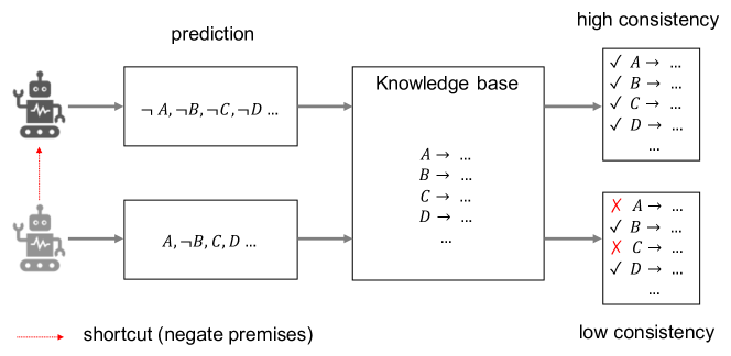
Figure 1: The implication bias is a tendency for NeSy systems to negate the premises of implication rules in order to increase consistency with the knowledge base.

Organization The organization of this paper is as follows. We begin by introducing the background of the field in section 3. In section 4, we present a formal definition of implication bias and provide a case study to explain this phenomenon. Our analysis demonstrates that implication bias is prevalent in NeSy logic loss functions derived from fuzzy operators. To address this issue, in section 5, we propose a simple yet effective method, Reduced Implication-bias Logic Loss (RILL). Finally, we empirically validate the effectiveness of RILL in section 6 by examining two challenging scenarios: the incomplete knowledge base and insufficient supervised data that we discussed earlier. This paper’s two main contributions are summarized as follows:

• We analyze the phenomenon of implication bias caused by differentiable implication operators and identify the loss functions that are susceptible to this bias.

• We propose a simple yet effective method called Reduced Implication-bias Logic Loss (RILL) to reduce implication bias. Empirical studies show that RILL can achieve significant improvements compared to other forms of logic loss, especially when the knowledge base is incomplete or labeled data is insufficient.

2 Related Work

Some researchers have attempted to design the structure of neural networks based on logical rules [30, 18, 15]. These structures embedded with logical constraints can perform well in specific tasks and satisfy their logic constraints. However, training such models requires a large amount of data.

Statistical Relational and Neural-Symbolic methods, such as DeepProbLog [20], TensorLog [4], and Abductive Learning (ABL) [36, 5], have been proposed to combine neural networks and logical programming. However, many of them attempt to approximately perform logical reasoning using distributed representations in neural networks, which typically require a tremendous amount of labeled data. Therefore, for simplicity, we do not consider differentiable operators implemented by parameter models, where a neural network acts as a logical reasoner. Although the use of neural networks for logical reasoning seems promising, it is beyond the scope of this paper.

A simple way to interact between the logical module and the perception module is to design a logic loss that measures how unsatisfying the model’s output is. As pointed out by Marra et al. [21], there are two perspectives on approximating logical reasoning with differentiable operations. From the perspective of probabilistic logic, [33] proposed a semantic loss function to obtain a logic loss. However, for efficient computation, they need to encode logical rules in Sentential Decision Diagrams (SDD) [6], which is an NP-hard problem and expensive for most real-world tasks. From the perspective of fuzzy logic, it is natural to use fuzzy operators to design logic losses, as demonstrated by several prior works [10, 29, 13, 1]. These works use fuzzy logic to translate logical rules into loss functions. Our work is closely related to [31], which analyzes different kinds of fuzzy logic operators and discovers a significant imbalance of gradients between premises and consequents in the Reichenbach operator.

3 Preliminaries

To provide context for our proposed method, we first present some concepts in logic programming. Next, we introduce the formal definition of continuous-valued logic, which forms the foundation for fuzzy-based logic loss in NeSy systems. Finally, we explain how logic loss is integrated with task-specific loss in NeSy systems.

3.1 Closed World Assumption

The closed-world assumption (CWA) [27] is a presumption that states if something is known to be true, it is considered true. If something is not currently known to be true, it is considered false. This is in contrast to the open-world assumption (OWA) [28], which holds that lack of knowledge does not imply falsity. The CWA is often used in database contexts, where information not explicitly presented in the database is assumed to be false. For example:

Statement:	Bob and Cam are students.
Question:	Is Alice a student?
Closed world answer:	No.
Open world answer:	Unknown.

Clark’s Completion Clark’s completion aims to address the problem caused by negating premises. By Clark’s Completion, the following knowledge base:

$$A\leftarrow A_{1},A\leftarrow A_{2},\cdots,A\leftarrow A_{n},$$

can be rewritten as $A\leftrightarrow(A_{1}\lor A_{2}\lor\cdots\lor A_{n})$, thus implementing the closed-world assumption and keeping the soundness of inference [3].

3.2 Continuous-valued Logic

Propositions are denoted as lowercase letters $x,y,z,\dots$, and propositional literals (i.e., $x,\neg x$) stand for $x$ being true or false. A term is a variable, a constant, or a function applied to terms. An atom (or atomic formula) is either a proposition or a predicate $p(t_{1},\cdots,t_{k})$ of arity k where the $t_{i}$ are terms. A formula is built out of atoms using logical connectives $\neg,\lor,\land,\rightarrow$, respectively. For simplicity, we assume that first-order-logic (FOL) formulas are universally quantified.

In this paper, we focus specifically on the problem caused by implication operators. Therefore, we will not discuss other types of operators for the sake of simplicity.

Definition 1 (Implication Likelihood).

An implication likelihood, or fuzzy implication, is a function $I(\cdot,\cdot):[0,1]^{2}\mapsto[0,1]$ that is differentiable and satisfies the following conditions: $I(0,0)=1$, $I(1,1)=1$, and $I(1,0)=0$.

Implication likelihood is a function that is used to estimate the truth-value of implication rules, which is closely related to fuzzy t-norms [13].

Definition 2 (Logic Likelihood).

A logic likelihood is a function $s(\cdot,\cdot):\mathbb{F}\times[0,1]^{n}\mapsto[0,1],$ that estimates the truth value of logic formulas.

The function $s(\cdot,\cdot)$ takes a logic formula and the corresponding truth-value vector as inputs. For instance, $s(P\rightarrow Q,(x,y))=I(x,y)$ evaluates the truth value of the rule $P\rightarrow Q$, where $x$ and $y$ represent the truth values of $P$ and $Q$, respectively.

Definition 3 ($\delta$-Confidence Monotonic).

A logic likelihood is said to be $\delta$-confidence monotonic if its implication likelihood satisfies the following property: for some $y\in[0,\delta)$, $I(x,y)$ is monotonically decreasing with respect to $x$.

To better understand this definition, let us consider the implication rule $\text{Raven}(x)\rightarrow\text{Black}(x)$. When the truth value of $\text{Black}(x)$ is almost 0 (i.e., $x$ is highly unlikely to be black), the truth value of this rule decreases as the confidence in $\text{Raven}(x)$ increases.

Functions with this property are commonly used in many publications [1, 29, 31]. For instance, the implication likelihood used in [1, 29] is defined as $I(x,y)=1-x+x\cdot y$, which is a $1$-confidence monotonic implication likelihood and is widely used in fuzzy-based NeSy systems. Furthermore, most fuzzy operators that serve as implication likelihoods exhibit this property, which we have shown in the appendix.

3.3 Logic Loss in NeSy Systems

Definition 4 (Logic Loss).

The logic loss $\ell_{\mathrm{logic}}$ is a function that estimates the inconsistency between a logic formula $r$ and a truth-value vector $\boldsymbol{z}$. It is defined as:

$$\ell_{\mathrm{logic}}(r,\boldsymbol{z})=g(s(r,\boldsymbol{z})),$$

where $g$ is a monotonically decreasing function with $g(1)=0$. For example, $g$ can be a negative logarithm function , such as $\ell_{\mathrm{logic}}(r,\boldsymbol{z})=1-\log(s(r,\boldsymbol{z})+1)$. In this paper, this function will be chosen as the default.

After we defined the individual logic loss for a single logical formula, the whole logic loss on the knowledge base and dataset (i.e. empirical logical risk) can be expressed as follows,

$$R_{\mathrm{logic}}(f)=\mathbb{E}_{\mathcal{X}\times\mathrm{KB}}[\ell_{\mathrm{logic}}(r,f(x)],$$

In addition to the logic loss, we also need to optimize the loss for a specific task:

$$R_{\mathrm{task}}(f)=\mathbb{E}_{\mathcal{X}\times\mathcal{Y}}[\ell_{\mathrm{task}}(f(x),y)].$$

We can combine these two parts to optimize:

$$f^{*}=\arg\max_{f}~{}[R_{\mathrm{task}}(f)+\lambda\cdot R_{\mathrm{logic}}(f)],$$

where $\lambda$ is a hyper-parameter of the training process.

Combining a logic loss with a task-specific loss in machine learning can be mutually beneficial. On the one hand, the task-specific loss can guide the model to achieve good performance and output valid logic primitive facts. On the other hand, the logic loss can help reduce the empirical optimal space and make the model easier to optimize.

However, as we will demonstrate in the next section, applying a logic loss with implication bias can introduce a significant bias into NeSy systems during the training process, which can make the optimization process more challenging.

4 Implication Bias

In this section, we will first give a formal definition of implication bias and discuss which types of logic loss are susceptible to this bias. We will then present a case study to illustrate this bias more clearly. Finally, we will further discuss implication bias from two perspectives.

4.1 Definition

Definition 5 (Implication Biased).

A logic loss is said to be implication biased if there exists a small $\delta>0$ such that its implication likelihood $I(x,y)$ satisfies $\forall x\in(0,\delta),\exists y\in[0,1],$

$$\frac{\partial I}{\partial x}<0.$$

Using this definition, we can state the following theorem.

Theorem 1.

A logic loss $\ell_{\mathrm{logic}}$ that uses a $\delta$-confidence monotonic logic likelihood is implication biased.

The proof follows directly from Definition 3. It is worth noting that logic likelihoods with $\delta$-confidence monotonicity are frequently used in many fuzzy-based NeSy systems (as we will demonstrate in the appendix), making this property pervasive in NeSy systems.

4.2 Case Study

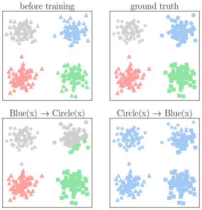
Figure 2: Case study of implication bias. These logic rules are both satisfied their logical constraints.

This case is designed to illustrate the impact of implication bias during the training process. The dataset is constructed from four clusters. Each data point in this dataset has two attributes:

color	$\in$	$\{\text{Blue, Green, Red, Gray}\}$
shape	$\in$	$\{\text{Circle, Square, Triangle, Star}\}.$

The attributes in our dataset are related to others according to the following logic rules: $\text{Blue}(x)\leftrightarrow\text{Circle}(x),\text{Green}(x)\leftrightarrow\text{Square}(x),\text{Gray}(x)\leftrightarrow\text{Star}(x),\text{Red}(x)\leftrightarrow\text{Triangle}(x)$.

The training set only contains the shape labels. The two different incomplete knowledge bases used in our experiments, shown in fig. 2, are ${\text{Blue}(x)\rightarrow\text{Circle}(x)}$ and ${\text{Circle}(x)\rightarrow\text{Blue}(x)}$.

For the task-specific loss, we use CrossEntropy, and for the logic loss, we use the Reichenbach Implication Likelihood, defined as $I(x,y)=1-x+x\cdot y$. The optimization objective is $R_{\mathrm{task}}(f)+\lambda\cdot R_{\mathrm{logic}}(f)$. The learning model is a one-hidden-layer neural network with two linear classification heads for shape and color.

As shown in the bottom left and right images of fig. 2, when the logic loss function is implication biased, the optimized model will avoid predicting any samples as blue, despite the initial model correctly predicting the color labels. This happens because the majority of the samples in the training set are unrelated to the single implication rule (i.e., they are neither blue nor circular). These samples will contribute significantly to the gradient towards negating the premise of the implication rule, causing the model to avoid predicting samples as blue.

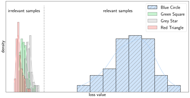
Figure 3: Distribution of different samples given by the loss values, which are computed from rule $\text{Circle}(x)\rightarrow\text{Blue}(x)$.

As can be seen in fig. 3, there is a significant difference in the distribution of logic loss between relevant and irrelevant samples for the rule $\text{Circle}(x)\rightarrow\text{Blue}(x)$. Even though the loss for irrelevant samples is relatively small, they still contribute a non-negligible amount to the gradient, which can negate the premise of the implication rule.

Remark It may be surprising that our model failed to correctly predict the shape labels in the bottom right image of fig. 2. This can happen because the logic loss function tends to favor negating the premise (i.e., vacuous truth caused by the implication bias), while the task-specific loss function is designed to favor the data or the goals of the task. As a result, the NeSy system may prioritize satisfying the logic loss function over achieving the goals of the task, leading to sub-optimal performance.

4.3 Analysis of Implication Bias

Let us analyze implication bias from two perspectives. Optimization The implication bias in neural networks can hinder the learning process by causing the networks to disregard the premise of implication rules, which are often used as shortcuts in the learning process. This bias may cause the network to perform sub-optimally. In many cases, a significant portion of the samples in a dataset does not meet the premise of a particular implication rule but rather satisfy the rule through vacuous truth (i.e., by negating the premise) [9]. When the logic loss is implication biased, these samples can still significantly contribute to the gradient, exacerbating the tendency to negate the premise of the implication rule and leading to even more biased results.

Logic Programming In an open world, negating a model’s prediction is undecidable. For instance, consider the statement $\textrm{Raven}(x)\rightarrow\textrm{Black}(x)$. In this case, there are many possible predicates that could be “not raven,” making it difficult to identify an explicit target for improving the model’s prediction.

Remark Implication bias poses a significant challenge for NeSy systems, particularly in the following two common and realistic scenarios:

• Incomplete knowledge base: In this case, there is missing or uncertain information that is necessary for making accurate inferences. This can make it difficult for the NeSy system to accurately approximate logical reasoning using differentiable operators.

• Insufficient supervised data: In this case, there is a small amount of labeled data available for training the NeSy system. This can make it difficult for the NeSy system to accurately learn from the data and make accurate predictions.

In the above cases, if the NeSy system is using loss functions that are susceptible to implication bias, this can further compound the problem. The bias introduced by these loss functions can cause the model to make inaccurate predictions and degrade its performance.

5 Reduce Implication Bias Logic Loss (RILL)

One possible approach to addressing the implication bias problem is to utilize a likelihood function that does not exhibit this bias. However, discovering such a function can be challenging and require extensive research. In this section, we introduce a simpler solution for reducing implication bias. We will begin by providing an overview of our approach, followed by a detailed explanation of our method and discussions for improved comprehension.

Insight Samples with low confidence in their premise should be assigned less importance:

• Samples with low confidence in their premise tend to have lower loss values, which means that they are less important to the optimization objective compared to other samples. Furthermore, these samples’ gradients can introduce a nuisance into the training process, so it is natural to reduce their importance.

• Samples with low confidence in their premise can introduce undecidability into the training process. Clark’s completion attempts to handle the undecidability of negative predicates by utilizing information explicitly present in the knowledge base. Therefore, it is natural to reduce the importance of information that is not explicitly present.

It is worth noting that low-loss value samples consist of two types. The first type includes samples that satisfy a specific rule and do not require backward tuning of the model’s parameters, leading to a low loss value. The second type comprises samples with low confidence in their premise, which we should assign less importance to. Therefore, we can consider low-loss value samples as irrelevant samples regarding a specific rule. Based on this, assigning importance to the samples can be straightforward, as we can assign different levels of importance based solely on their loss value.

Consider all samples’ individual logic loss on a formula $r$ and rank them by their loss value (from low to high):

$$\underbrace{\ell_{1}^{r},\ell_{2}^{r},\cdots,\ell_{t}^{r}}_{\text{weak samples}},\cdots,\ell_{N}^{r}.$$

The “weak samples” referred to in the equation are those with low loss values, such as irrelevant samples depicted in fig. 3. These weak samples are generally considered less reliable than the other samples when applying the given rule. To distinguish between weak and non-weak samples, we can use a threshold $\epsilon$ to divide them.

Without losing generality, we can rewrite the risk of logic in the following form:

$$R_{\textrm{logic}}=\sum_{r\in\textrm{KB}}\mathcal{A}(\left\{\ell_{i}^{r}|i\in[N]\right\}),$$

where the aggregator $\mathcal{A}$ is typically used to average the losses. One way to reduce bias in the results is to redefine the aggregator to give less weight to weak samples. Let $\mathcal{L}^{r}$ be the set of losses $\left\{\ell_{i}^{r}|i\in[N]\right\}$. We propose three possible aggregators as follows.

Hinge One option for reducing bias in the results is to use a hinge-like aggregator, which ignores the losses of weak samples.

$$\mathcal{A}_{\textit{hinge}}(\mathcal{L}^{r})=\textrm{Average}(\left\{\ell_{i}^{r}|\ell_{i}^{r}\geq\epsilon,i\in[N]\right\})$$

This aggregator can be viewed as a form of sample selection, as it only includes the loss values of non-weak samples in the computation. It is similar to the RAMP loss function [25], which also only considers a subset of samples for robust optimization.

L2 Smooth Since we want to reduce the bias caused by weak samples’ gradients of biased logic loss, it is natural to smooth by multiplying itself.

$$\mathcal{A}_{\textit{l2}}(\mathcal{L}^{r})=\textrm{Average}(\left\{(\ell_{i}^{r})^{2}|i\in[N]\right\})$$

The aggregator in this method smooths the biased logic loss by multiplying it with itself, giving lower-loss samples a smoother gradient and reducing the bias of weak samples. This can be seen in the equation $\nabla\ell^{2}=2\ell\nabla\ell$.

L2+Hinge Kind of mixing the above aggregators:

$$\mathcal{A}_{\textit{l2+hinge}}(\mathcal{L}^{r})=\textrm{Average}(\left\{\mathcal{T}(\ell_{i}^{r})|i\in[N]\right\}),$$

where

$$\mathcal{T}(\ell)=\ell^{2}\cdot\mathbb{I}[\ell\leq\epsilon]+\ell\cdot\mathbb{I}[\ell>\epsilon].$$

Remark The solutions described above aim to reweight the samples based on their loss value, which reflects their relevance to an implication rule. While we have presented three specific aggregators for achieving this, it is worth noting that other approaches that similarly aim to reduce the influence of weak samples could also be effective in addressing this issue.

Discussion RILL reduces the uncertainty associated with negative information, similar to Clark’s completion. While RILL does not alter the information in the knowledge base but instead reduces the importance of weak samples. This reduction causes the model to pay more attention to samples that are more relevant to the given rule.

On the other hand, explicitly applying Clark’s completion in a NeSy system may not be helpful. In this setting, replacing $\rightarrow$ with $\leftrightarrow$ would change the information in the knowledge base, potentially leading to incorrect information. While Clark’s completion does not affect the soundness of the system in logic programming, it may not be the case in a data-driven approach such as NeSy. More discussion on the relationship between RILL and Clark’s completion can be found in the appendix.

6 Empirical Study

In this section, we will discuss two common challenges that occur in real-world scenarios: incomplete knowledge bases and insufficient supervised data. We will begin by briefly introducing the compared methods. Next, we will set up the experiments. Finally, we empirically validate the performance of RILL and other compared methods under these settings.

6.1 Setting Up

The compared methods come from two mainstream perspectives of NeSy systems. From the fuzzy logic perspective, the logic loss derived from Reichenbach operators outperforms other methods, as reported in [31]. From the probabilistic logic perspective, we chose the semantic loss (SL for short) [33] due to its well-defined nature and efficiency. The following definition is taken from [33].

Definition 6 (Semantic Loss).

Let $\mathrm{p}$ be a vector of probabilities, one for each variable in $\mathbf{X}$, and let $\alpha$ be a sentence over $\mathbf{X}$. The semantic loss between $\alpha$ and $\mathrm{p}$ is defined as:

$$\mathrm{L}^{\mathrm{s}}(\alpha,\mathrm{p})\propto-\log\sum_{\mathbf{x}\models\alpha}\prod_{i:\mathbf{x}\models X_{i}}\mathrm{p}{i}\prod{i:\mathbf{x}\models\neg X_{i}}\left(1-\mathbf{p}_{i}\right).$$

In the optimization process, the logic loss is calculated based on rules in the knowledge base and the training data, which includes both labeled and unlabeled data. The task-specific loss, on the other hand, is only calculated using the labeled data in the training set.

Since this paper focuses on NeSy systems based on loss functions, we do not consider other types of NeSy systems. Additionally, we present a method that does not rely on any information from the knowledge base, which we refer to as “Vanilla” in the following table. More details about the experiments and their configurations can be found in the appendix.

6.1.1 Task 1 Addition Equations

Inspired by Hoernle et al. [15], we constructed a semi-supervised-like task that uses a small number of labeled data and a large amount of well-structured unlabeled data to train a machine learning model. Specifically, the data is structured by additive equations, as shown in fig. 4. This structure can be applied to datasets with ten classes, not just digit datasets. In our experiments, we use MNIST [8], FashionMNIST [32], and CIFAR-10 [17] as basic datasets, which we organize as illustrated in fig. 4. We use three-layer Multi-layer Perceptron (MLP) models for MNIST/FashionMNIST and ResNet9 [14] for CIFAR-10. The task-specific loss for this task is CrossEntropy.

Figure 4: Addition Equation Experiment, data are structured with equation constraints. All adopted equations in this experiment consist of four digits. For instance, in this picture, $1+5=06$.

Knowledge Base Addition equations with four digits have $10\times 10=100$ rules. For example, rules $5+2=07,5+3=08$ can be represented as:

$\text{1stD5}(x_{1})\land\text{2ndD2}(x_{2})\rightarrow$	$\text{3thD0}(x_{3})\land\text{4thD7}(x_{4})$
$\text{1stD5}(x_{1})\land\text{2ndD3}(x_{2})\rightarrow$	$\text{3thD0}(x_{3})\land\text{4thD8}(x_{4}).$

Task 1 is well suited to validate the performance of NeSy systems in the scenario of incomplete knowledge bases since its structure allows for strong constraints to be imposed during learning. Specifically, logic loss of this task can correct misclassified labels when most digits are recognized correctly. This adaptability to varying amounts of labeled data also makes it suitable for scenarios with limited supervised data.

6.1.2 Task 2 Hierarchical Classification

CIFAR-100 [17] consists of 100 classes and 20 super-classes (SC). For example, an image can be classified with a class label of maple and a super-class label of trees. In this experiment, we utilize the relationships between classes and super-classes. We adopt the WideResNet28-8 [35] model as the backbone, with two linear classification heads for the class label and super-class label. The task-specific loss for this experiment is CrossEntropy.

Knowledge Base Knowledge rules in this task are relationships between classes and super-classes, such as:

$\text{Aquarium fish}(x)\rightarrow$	$\text{Fishes}(x)$
$\text{Shark}(x)\rightarrow$	$\text{Fishes}(x).$

Task 2 has a weaker knowledge base than Task 1. In this task, even if the model correctly predicts the super-class, the knowledge base does not provide precise information on how to correct wrongly predicted sub-classes. Therefore, this task mainly focuses on scenarios with insufficient supervised data.

6.2 Incomplete Knowledge Base

When the knowledge base is incomplete, implication bias can be a significant issue for NeSy systems. This is because the model may not have access to all the relevant knowledge for making accurate reasoning and may instead rely more on vacuous truth. As a result, the model may perform poorly.

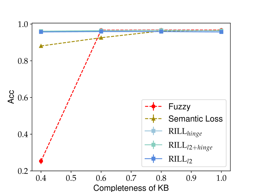
(a) Add-MNIST

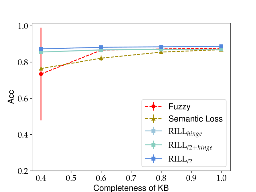
(b) Add-FashionMNIST

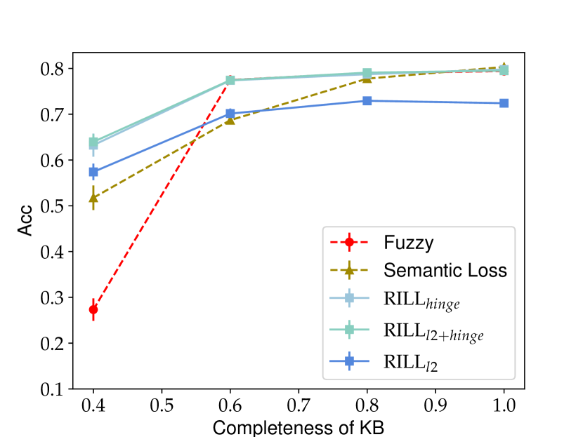
(c) Add-CIFAR10

Figure 5: Effect of incomplete knowledge base: In this case, models may not have access to all the relevant knowledge for making accurate reasoning.

The completeness of knowledge bases ranges from 100% to 40%, i.e., the number of rules in knowledge bases varies from 100 to 40. The size of the labeled dataset used in this task is 100 for MNIST and FashionMNIST and 2000 for CIFAR-10. In Figure 5, it is illustrated that as the degree of completeness decreases, the model’s performance tends to decline as well.

Analysis The RILL approach is more stable and performs better than other methods, particularly when the knowledge base is incomplete. This is because RILL assigns less importance to weak samples, which helps reduce the impact of implication bias. Thus, RILL is a useful approach for dealing with incomplete knowledge bases and mitigating the effects of implication bias.

6.3 Insufficient Supervised Data

Insufficient supervised data can hinder the NeSy system’s ability to learn and make accurate predictions. This is because there may not be enough examples to learn from and generalize to new cases. Using loss functions that are prone to implication bias can exacerbate this problem. The experimental results for this scenario are shown in fig. 6, table 1, and table 2.

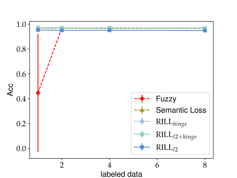
(a) Add-MNIST

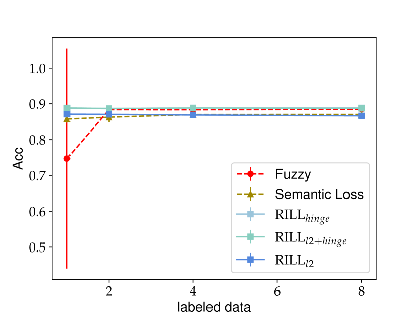
(b) Add-FashionMNIST

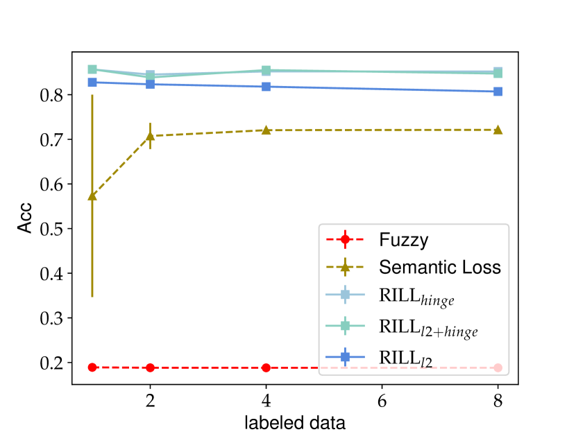
(c) Add-CIFAR10

Figure 6: Effect of insufficient supervised data: In this case, the system may not have enough examples to learn from and generalize to new cases

supervised data	8	4	2	1
Fuzzy	0.1891$\pm$0.001	0.1906$\pm$0.004	0.1902$\pm$0.002	0.1904$\pm$0.001
SL	0.7266$\pm$0.009	0.7200$\pm$0.003	0.7316$\pm$0.049	0.6785$\pm$0.024
$\textrm{RILL}{l2}$	0.8502$\pm$0.005	0.8560$\pm$0.003	0.8473$\pm$0.015	0.8582$\pm$0.004
$\textrm{RILL}{l2+hinge}$	0.8139$\pm$0.012	0.8202$\pm$0.004	0.8265$\pm$0.005	0.8316$\pm$0.006
$\textrm{RILL}_{hinge}$	0.8548$\pm$0.005	0.8573$\pm$0.011	0.8481$\pm$0.007	0.8581$\pm$0.003

Table 1: Effect of insufficient supervised data: Task1, Add-CIFAR-10, showing accuracies for different amounts of supervised data. Experiments were repeated five times. The boldface entries denote the best results, according to the Wilcoxon signed-rank test at the 5% significance level.

Task 1 The size of the labeled dataset decreases from eight to one sample per class. As shown in fig. 6, the fuzzy logic loss struggles to improve the model’s performance when the dataset is small, due to the difficulty of making accurate predictions and the effects of implication bias, particularly in the more challenging Add-CIFAR-10 task (c.f., table 1). However, RILL performs much better because it assigns less weight to weak samples, which helps mitigate the impact of implication bias. It’s worth noting that RILL was able to achieve an 86% accuracy on CIFAR-10 using only one labeled sample per class.

supervised data	10		1
	Acc	SC-Acc	Acc	SC-Acc
Fuzzy	0.4449$\pm$0.010	0.7585$\pm$0.014	0.2291$\pm$0.004	0.7484$\pm$0.014
SL	0.4310$\pm$0.034	0.7462$\pm$0.037	0.2281$\pm$0.007	0.7384$\pm$0.021
Vanilla	0.4520$\pm$0.004	0.7670$\pm$0.010	0.2297$\pm$0.007	0.7415$\pm$0.014
$\text{RILL}_{l2+hinge}$	0.4509$\pm$0.002	0.7649$\pm$0.008	0.2363$\pm$0.009	0.7575$\pm$0.004
$\text{RILL}_{l2}$	0.4538$\pm$0.003	0.7699$\pm$0.005	0.2357$\pm$0.010	0.7449$\pm$0.014
$\text{RILL}_{hinge}$	0.4562$\pm$0.004	0.7750$\pm$0.006	0.2334$\pm$0.006	0.7463$\pm$0.014

Table 2: Effect of insufficient supervised data: Task2, Hierarchical-Classification showing accuracies for different amounts of supervised data. Experiments were repeated five times. The boldface entries denote the best results according to the Wilcoxon signed-rank test at the 5% significance level.

Task 2 The size of the class-labeled dataset decreases from ten to one sample per class. As shown in table 2, RILL maintains relatively high performance (both acc and sc-acc) and stability (indicated by std) compared to other methods, particularly when the labeled dataset is small. This highlights the importance of reducing implication bias.

Remark One may be surprised to see that the performance of our model slightly improved as the size of the labeled data decreased (see fig. 6). This may be similar to the smooth label effect discussed in [22]. However, this phenomenon only appears in Task 1 and not in Task 2 because the knowledge base used in Task 2 is weaker and does not provide precise instructions for correcting misclassified sub-classes. This is likely why RILL is less effective in Task 2.

7 Discussion and Limitation

Discussion The results of the experiments show that $\textrm{RILL}_{l2}$ performs worse than the other types of RILL. This is because the $l2$ aggregator gives equal weight to all samples by multiplying their loss values, while the hinge and l2+hinge aggregators use a hard threshold to reduce the influence of weak samples. Therefore, the latter two aggregators can reduce bias more effectively if an appropriate threshold is chosen.

Implication bias may not be a problem in NeSy systems if the following conditions are met: complete knowledge base, sufficient supervised data, and robust training methods. The extent to which implication bias affects a NeSy system will depend on the task and training methods. In general, it is important to consider the potential impact of implication bias and take steps to mitigate it if necessary.

Limitation This work has two limitations. First, it only computes the logic loss from each individual logic rule in the knowledge base and does not consider the complex interactions between different rules. Future work could involve measuring complex reasoning processes using loss functions. Second, the discussion of weak samples requires further investigation. This topic is related to learning with noisy labels [23], and identifying these samples remains a key problem in this field.

8 Conclusion

This paper analyzes implication bias, which is a tendency for NeSy systems to shortcut the logic of implication rules by negating the premise. The paper discusses the cause and negative effects of implication bias and confirms its existence through experiments. We propose Reduced Implication-bias Logic Loss (RILL) as a solution. RILL reduces the uncertainty of negative information by lowering the importance of weak samples and causing the model to pay more attention to relevant samples. Empirical studies show that RILL can improve performance and increase robustness compared to other forms of logic loss, especially in cases of incomplete knowledge bases or insufficient supervised data.

Appendix A Discussion with other kinds of fuzzy operators

In this section, we investigate different types of fuzzy operators and experimentally validate their effectiveness while maintaining the implication biased. When selecting fuzzy operators for NeSy, it is crucial to consider their smoothness and ease of optimization. Therefore, we concentrate on commonly used fuzzy operators that possess these desirable properties. Fuzzy operators that do not have a smooth gradient will be disregarded in our analysis.

A.1 Analysis

Sigmoidal van Krieken et al. [31] proposed an operator which is smoothed Reichenbach operator by a sigmoid function. This implication likelihood function is defined as follows:

$$\sigma_{I}(p,q)=\frac{1+e^{-s\left(1+b_{0}\right)}}{e^{-b_{0}s}-e^{-s\left(1+b_{0}\right)}}\cdot\left(\left(1+e^{-b_{0}s}\right)\cdot\sigma\left(s\cdot\left(I(p,q)+b_{0}\right)\right)-1\right),$$

where $s>0,b_{0}\in\mathbb{R},\sigma(\cdot)=\frac{1}{1+e^{x}}$ denotes the sigmoid function. Substituting $d=\frac{1+e^{-s\left(1+b_{0}\right)}}{e^{-b_{0}s}-e^{-s\left(1+b_{0}\right)}},h=(1+e^{-s\cdot b_{0}}),f=\sigma\left(s\cdot\left(I(p,q)+b_{0}\right)\right)$, we find:

$$\frac{\partial\sigma_{I}(p,q)}{\partial I(p,q)}=d\cdot h\cdot s\cdot f\cdot(1-f)>0.$$

That is to say when $I(p,q)$ is $\delta$-Confidence Monotonic, $\sigma_{I}(p,q)$ will be $\delta$-Confidence Monotonic too. This means logic loss derived from $\sigma_{I}$ will become implication biased.

Łukasiewicz Łukasiewicz implication likelihood [2] was defined as follows:

$$I_{LK}(p,q)=\min(1-p+q,1).$$

It is easy to calculate the gradient of this likelihood, $\frac{\partial I_{LK}}{\partial p}=-1\cdot\mathbb{I}[p>q]$. It turns out this is also implication biased.

G$\ddot{\text{o}}$del G$\ddot{\text{o}}$del implication likelihood [24] was defined as follows:

$$I_{G}(p,q)=\max(1-p,q).$$

Also, the gradient of this likelihood $\frac{\partial I_{G}}{\partial p}=-1\cdot\mathbb{I}[p+q<1]$ indicates this operator is implication biased.

Nilpotent Nilpotent implication likelihood [12] was defined as follows:

$$I_{N}(p,q)=\left\{\begin{aligned} &1,&\mathrm{if}\quad p\leq q.\\ &\max(1-p,q),&\mathrm{otherwise}.\end{aligned}\right.$$

Also, the gradient of this likelihood $\frac{\partial I_{N}}{\partial p}=-1\cdot\mathbb{I}[(p+q<1)\&(p>q)]$ indicates this operator is implication biased.

A.2 Empirical Study

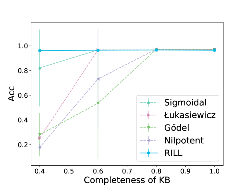
(a) Incomplete knowledge base

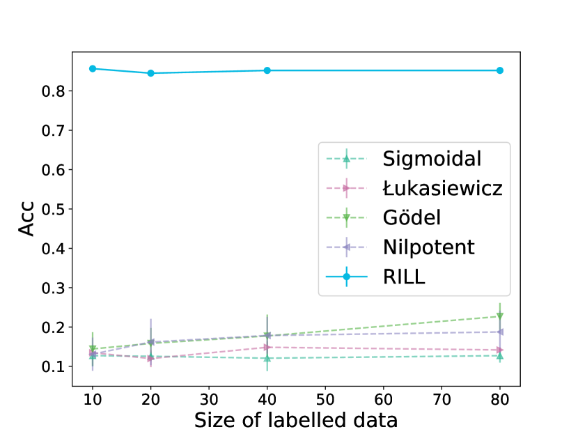
(b) Insufficient supervised data

Figure 7: Verification of implication bias across various fuzzy operators is crucial. The empirical evidence illustrated in the preceding images substantiates our assertion that this phenomenon is pervasive.

In this section, we present the empirical results of the above-analyzed operators for validation, with a particular emphasis on incomplete knowledge bases (especially Add-MNIST) and insufficient labeled data (especially Add-CIFAR10) scenarios. All experiments follow the same settings used in section 6.1.1.

As shown in fig. 7, implication bias significantly harms the performance of the model, especially when the knowledge base is incomplete or the amount of supervised information is not sufficient, which further supports our above analysis.

Appendix B Discussion about Clark’s Completion

RILL and Clark’s completion both aim to reduce the uncertainty of negative information. While RILL does not alter the information in the knowledge base, but instead reduces the importance of weak samples, causing the model to pay more attention to samples that are more relevant to the given rule.

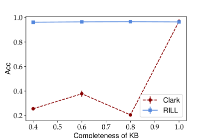
Figure 8: Performance of Clark’s Completion drops when the completeness of KB is decreasing.

Surprisingly, explicitly applying Clark’s completion in a NeSy system may not be helpful. There are two reasons behind this claim.

First, a explicitly Clark’s completion need to replace $\rightarrow$ to $\leftrightarrow$. For example:

$$A\leftarrow A_{1},A\leftarrow A_{2},\cdots,A\leftarrow A_{n},$$

will be replaced as $A\leftrightarrow(A_{1}\lor A_{2}\lor\cdots\lor A_{n})$.

However, the fuzzy operator is unsuitable for approximating a rule with many atoms [21]. An example is the n-ary Łukasiewicz strong disjunction $F_{\lor}(x_{1},\cdots,x_{n})=\min(1,x_{1}+\cdots+x_{n})$. Although all $x_{i}$ can be very small, this approximation of disjunction will give a value near 1. Because Clark’s completion will increase the number of atoms in the logical rule, the knowledge base may suffer from this problem after completion.

Second, in a NeSy system, if the knowledge base is incomplete, replace $\rightarrow$ to $\leftrightarrow$ will change the information in the knowledge base, which may induce wrong information. In logic programming, Clark’s completion will not change the soundness of the system, while in the NeSy setting with a data-driven approach, it may not be promised.

Here we adopt the same experimental setting of incomplete knowledge base case in section 6.1.1 to validate the performance of Clark’s Completion. As depicted in fig. 8, when the knowledge base becomes incomplete, completion of the knowledge base will not help improve the model’s performance because it introduces wrong information.

Appendix C Sensitivity Analysis

Both $\text{RILL}_{hinge}$ and $\text{RILL}_{l2+hinge}$ contain a hyper-parameter $\epsilon$ in their definition. In this section, we investigate the sensitivity of $\epsilon$ and its impact on the model’s accuracy in the Add-MNIST experiment when the knowledge base incompleteness is 40%. fig. 9 displays the relationship between $\epsilon$ and the model’s accuracy.

The results indicate that when the threshold $\epsilon$ decreases to a certain value (in fig. 9, it is 0.001), the model’s performance drops, suggesting the existence of a sensitive region that could be related to weak samples in addressing the problem of implication bias. When the threshold $\epsilon$ is above this value, the performance of RILL is stable but slightly decreasing. This decrease may be due to the increased number of weak samples, which results in the loss of some useful information.

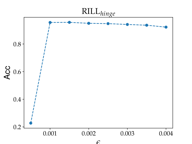
(a) $\text{RILL}_{hinge}$

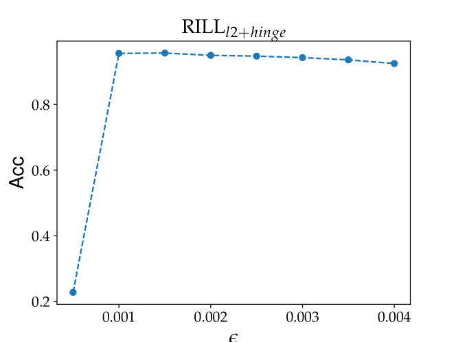
(b) $\text{RILL}_{l2+hinge}$

Figure 9: Sensitivity Analysis of the hyper-parameter $\epsilon$.

Appendix D Details of Experiments

In this section, we will provide more details of our experiments. Implementation of Semantic Loss The formal definition of Semantic Loss requires the conversion of CNF (conjunctive normal form) into SDD (sentential decision diagram), which can become impractical when dealing with knowledge bases that use a large number of predicates and complex rules due to the heavy computational burden. To address this issue, we propose an alternative approach where each rule in the knowledge base is converted separately into wmc (weighted model counting) models and then combined at the end. Although explicit repetitive terms are reduced during the combining phase, detecting implicit repetitive terms is computationally expensive, and thus they remain unchanged. This approach enables us to implement Semantic Loss efficiently while still accounting for the complexity of the knowledge base.

However, even with this optimization, the cost of using Semantic Loss is still much higher than that of using RILL, with a cost that is around three times higher. As a result, Semantic Loss may not be practical to use in many cases, particularly when dealing with large or complex knowledge bases.

Details of Task 1 The backbone for both MNIST and FashionMNIST datasets is a three-layer Multilayer Perceptron (MLP) with a width of each layer being [256,512,10], and the activation function is Rectified Linear Unit (ReLU) [19]. In contrast, the backbone for CIFAR10 is ResNet9 [14]. The value of $\lambda$ for both Fuzzy and RILL logic loss is 0.7. For Semantic Loss, we sample $\lambda$ from $\{0.001,0.005,0.01,0.05,0.1,0.5\}$ and choose the best one, which is 0.5 in this experiment. The learning rate is set to 0.0001, with a decay rate of 0.7. The learning rate scheduler is set to StepLR, with a decay step of 60. The optimizer used is AdamW as default, and the weight decay rate is set to 5e-4.

Details of Task 2 For this task, we select WideResNet-28-8 [35] as the backbone architecture with two classification heads, one for class classification, and the other for super-class classification. The value of $\lambda$ for both Fuzzy and RILL logic loss is 0.002, and for Semantic Loss, we still choose 0.5 as the default value. The learning rate is set to 0.005, with a decay rate of 0.9 and decay steps equal to 45. The learning rate scheduler is set to StepWithWarmUp, and the warm-up epoch is set as 5. The optimizer used is set as default, and momentum is set to 0.9.

Availability of data and material All datasets are publicly available. Code availability Available at https://git.nju.edu.cn/Alkane/clion.git. Author’s contributions H conceived the central idea of this paper and contributed to the writing and execution of the main experiments. D contributed to the enhancement of the RILL approach and the refinement of this paper. L provided valuable feedback, suggestions, and editing services for this manuscript.

Declarations

Funding Not applicable. Conflicts of interest Not applicable. Ethics approval Not applicable. Consent to participate Not applicable. Consent for publication Not applicable.

References

- Badreddine et al. [2022] Samy Badreddine, Artur S. d’Avila Garcez, Luciano Serafini, and Michael Spranger. Logic tensor networks. Artificial Intelligence Journal, 2022. 10.1016/j.artint.2021.103649.
- Cignoli [2007] Roberto Cignoli. The Algebras of Łukasiewicz Many-Valued Logic: A Historical Overview. 2007. 10.1007/978-3-540-75939-3_5.
- Clark [1978] Keith L Clark. Negation as failure. In Logic and data bases, pages 293–322. 1978.
- Cohen et al. [2020] William W. Cohen, Fan Yang, and Kathryn Mazaitis. Tensorlog: A probabilistic database implemented using deep-learning infrastructure. Journal of Artificial Intelligence Research, 2020. 10.1613/jair.1.11944.
- Dai et al. [2019] Wang-Zhou Dai, Qiu-Ling Xu, Yang Yu, and Zhi-Hua Zhou. Bridging machine learning and logical reasoning by abductive learning. In Conference on Neural Information Processing Systems, 2019.
- Darwiche [2011] Adnan Darwiche. SDD: A new canonical representation of propositional knowledge bases. In International Joint Conference on Artificial Intelligence, pages 819–826, 2011.
- d’Avila Garcez et al. [2019] Artur S. d’Avila Garcez, Marco Gori, Luís C. Lamb, Luciano Serafini, Michael Spranger, and Son N. Tran. Neural-symbolic computing: An effective methodology for principled integration of machine learning and reasoning. Journal of Applied Logics, 2019.
- Deng [2012] Li Deng. The MNIST database of handwritten digit images for machine learning research. IEEE Signal Processing Magazine, 2012. 10.1109/MSP.2012.2211477.
- Enderton [1972] Herbert B. Enderton. A mathematical introduction to logic. 1972.
- Fischer et al. [2019] Marc Fischer, Mislav Balunovic, Dana Drachsler-Cohen, Timon Gehr, Ce Zhang, and Martin T. Vechev. DL2: training and querying neural networks with logic. In International Conference on Machine Learning, 2019.
- Geirhos et al. [2020] Robert Geirhos, Jörn-Henrik Jacobsen, Claudio Michaelis, Richard S. Zemel, Wieland Brendel, Matthias Bethge, and Felix A. Wichmann. Shortcut learning in deep neural networks. Nat. Mach. Intell., 2020. 10.1038/s42256-020-00257-z.
- Gerla and Rovere [2011] Brunella Gerla and Massimo Dalla Rovere. Nilpotent minimum fuzzy description logics. In European Society for Fuzzy Logic and Technology, 2011. 10.2991/eusflat.2011.127.
- Giannini et al. [2019] Francesco Giannini, Giuseppe Marra, Michelangelo Diligenti, Marco Maggini, and Marco Gori. On the relation between loss functions and t-norms. In International Conference on Inductive Logic Programming, 2019. 10.1007/978-3-030-49210-6_4.
- He et al. [2016] Kaiming He, Xiangyu Zhang, Shaoqing Ren, and Jian Sun. Deep residual learning for image recognition. In IEEE Conference on Computer Vision and Pattern Recognition, 2016. 10.1109/CVPR.2016.90.
- Hoernle et al. [2022] Nick Hoernle, Rafael-Michael Karampatsis, Vaishak Belle, and Kobi Gal. Multiplexnet: Towards fully satisfied logical constraints in neural networks. In AAAI Conference on Artificial Intelligence, 2022.
- Klement et al. [2013] E.P. Klement, R. Mesiar, and E. Pap. Triangular Norms. 2013.
- Krizhevsky et al. [2009] Alex Krizhevsky, Geoffrey Hinton, et al. Learning multiple layers of features from tiny images. Technical Report TR 2009, 2009.
- Li and Srikumar [2019] Tao Li and Vivek Srikumar. Augmenting neural networks with first-order logic. In Anna Korhonen, David R. Traum, and Lluís Màrquez, editors, Annual Meeting of the Association for Computational Linguistics, 2019. 10.18653/v1/p19-1028.
- Maas et al. [2013] Andrew L Maas, Awni Y Hannun, Andrew Y Ng, et al. Rectifier nonlinearities improve neural network acoustic models. In International Conference on Machine Learning, 2013.
- Manhaeve et al. [2018] Robin Manhaeve, Sebastijan Dumancic, Angelika Kimmig, Thomas Demeester, and Luc De Raedt. Deepproblog: Neural probabilistic logic programming. In Conference on Neural Information Processing Systems, 2018.
- Marra et al. [2021] Giuseppe Marra, Sebastijan Dumancic, Robin Manhaeve, and Luc De Raedt. From statistical relational to neural symbolic artificial intelligence. CoRR, 2021.
- Müller et al. [2019] Rafael Müller, Simon Kornblith, and Geoffrey E. Hinton. When does label smoothing help? In Conference on Neural Information Processing Systems, 2019.
- Natarajan et al. [2013] Nagarajan Natarajan, Inderjit S. Dhillon, Pradeep Ravikumar, and Ambuj Tewari. Learning with noisy labels. In Conference on Neural Information Processing Systems, 2013.
- Paad [2016] Akbar Paad. Relation between (fuzzy) gödel ideals and (fuzzy) boolean ideals in bl-algebras. Discussiones Mathematicae General Algebra and Applications, 2016.
- Phoungphol et al. [2012] Piyaphol Phoungphol, Yanqing Zhang, and Yichuan Zhao. Robust multiclass classification for learning from imbalanced biomedical data. Tsinghua Science and technology, (6):619–628, 2012.
- Raedt et al. [2020] Luc De Raedt, Sebastijan Dumancic, Robin Manhaeve, and Giuseppe Marra. From statistical relational to neuro-symbolic artificial intelligence. In International Joint Conference on Artificial Intelligence, 2020. 10.24963/ijcai.2020/688.
- Reiter [1978] Raymond Reiter. On Closed World Data Bases. 1978. 10.1007/978-1-4684-3384-5_3.
- Reiter [1980] Raymond Reiter. A logic for default reasoning. AI, 1980. 10.1016/0004-3702(80)90014-4.
- Roychowdhury et al. [2021] Soumali Roychowdhury, Michelangelo Diligenti, and Marco Gori. Regularizing deep networks with prior knowledge: A constraint-based approach. Knowledge-Based System, 2021. 10.1016/j.knosys.2021.106989.
- Towell and Shavlik [1994] Geoffrey G. Towell and Jude W. Shavlik. Knowledge-based artificial neural networks. Artificial Intelligence Journal, 1994.
- van Krieken et al. [2022] Emile van Krieken, Erman Acar, and Frank van Harmelen. Analyzing differentiable fuzzy logic operators. Artificial Intelligence Journal, 2022. 10.1016/j.artint.2021.103602.
- Xiao et al. [2017] Han Xiao, Kashif Rasul, and Roland Vollgraf. Fashion-mnist: a novel image dataset for benchmarking machine learning. CoRR, 2017.
- Xu et al. [2018] Jingyi Xu, Zilu Zhang, Tal Friedman, Yitao Liang, and Guy Van den Broeck. A semantic loss function for deep learning with symbolic knowledge. In International Conference on Machine Learning, 2018.
- Yang et al. [2022] Zhun Yang, Joohyung Lee, and Chiyoun Park. Injecting logical constraints into neural networks via straight-through estimators. In International Conference on Machine Learning, 2022.
- Zagoruyko and Komodakis [2016] Sergey Zagoruyko and Nikos Komodakis. Wide residual networks. In British Machine Vision Conference, 2016.
- Zhou [2019] Zhi-Hua Zhou. Abductive learning: towards bridging machine learning and logical reasoning. Science China Information Sciences, 2019. 10.1007/s11432-018-9801-4.