Dynamic Brillouin cooling for continuous optomechanical systems

Abstract

In general, ground state cooling using optomechanical interaction is realized in the regime where optical dissipation is higher than mechanical dissipation. Here, we demonstrate that optomechanical ground state cooling in a continuous optomechanical system is possible by using backward Brillouin scattering while mechanical dissipation exceeds optical dissipation which is the common case in optical waveguides. The cooling is achieved in an anti-Stokes backward Brillouin process by modulating the intensity of the optomechanical coupling via a pulsed pump to suppress heating processes in the strong coupling regime. With such dynamic modulation, a cooling factor with several orders of magnitude can be realized, which breaks the steady-state cooling limit. This modulation scheme can also be applied to Brillouin cooling generated by forward intermodal Brillouin scattering.

Introduction.—Cooling a mechanical oscillator to its ground state by overcoming the effects of thermal environment has always attracted great interests, as it offers attractive opportunities for various topics including high precision metrology LaHaye ; Teufel1 ; Purdy , quantum information processing Palomaki ; Riedinger ; Ockeloen-Korppi , and the exploration of classical-and-quantum limit of macroscopic objects Marshall ; Pikovski ; Arndt . Preparing a single mode mechanical oscillator into its quantum ground state has been experimentally realized in cavity optomechanical systems by utilizing methods in combination with optomechanical radiation pressure interactions Teufel2 ; Chan ; Liu ; Aspelmeyer . Apart from optomechanical radiation pressure interaction, optoacoustic Brillouin interaction induced by electrostrictive effects Boyd ; Agrawal provides a potential mechanical cooling method for cavity optomechanical systems Matthew ; Matthew2 ; Bahl ; Chunhua ; Chunhua2 ; Enzian and continuous optomechanical systems Chen ; Otterstrom . For both kinds of systems, nevertheless, Brillouin cooling has so far only been studied for optical forward scattering. In particular for a continuous waveguide system, forward Brillouin cooling has been investigated theoretically Chen as well as experimentally Otterstrom . However, Brillouin cooling generated by backward scattering and cooling traveling-wave acoustic phonons close to or even well into quantum ground state in continuous optomechanical systems are still open questions.

Recently, a variety of integrated optomechanical waveguides at small size scales ($\sim$cm or mm length) were realized in experiment Eggleton . These short Brillouin-active waveguides with high Brillouin gain allow the coherent light-sound interaction in a small regime, which enables the dynamical control of photonic-phononic interaction through a pulsed laser such as coherent photonic-phononic memory Merklein . In addition, it has been theoretically predicted that the strong coupling regime of the anti-Stokes Brillouin interaction can be accessible in highly nonlinear waveguides Laer1 ; Huy . The strong optomechanical interaction permits state swapping between photons and phonons Verhagen ; Naeini which is one way to achieve phonon cooling Hensinger ; TianLin ; TianLin2 ; Xiaoting ; Yongchun . As a consequence, a Brillouin cooling scheme that can beat the phonon heating rate for continuous optomechanical systems coupled with the environment is highly desirable by manipulating the dynamics of photonic-phononic interaction in integrated waveguides.

In this work, we demonstrate that one can achieve a great cooling factor via backward Brillouin scattering in continuous optomechanical systems under the strong coupling regime. By periodically modulating the optomechanical coupling strength through a pulsed laser, the heating generated by the state swapping and thermal noise can be significantly suppressed, which enables the phonon occupancy to reach an

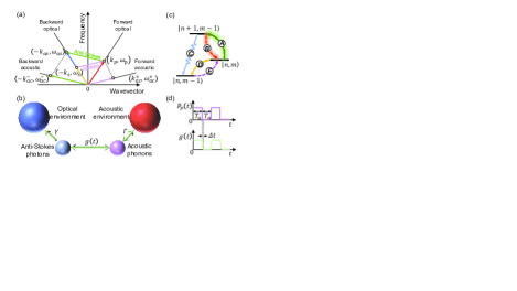
Figure 1: (color online) (a) Sketch of a typical dispersion diagram of backward Brillouin scattering for both Stokes and anti-Stokes processes. Subscripts of ‘$p$’, ‘$as$’, ‘$s$’ correspond to optical pump, anti-Stokes, Stokes fields and ‘$ac$’ indicates acoustic field, respectively. Superscripts ‘$-$’ and ‘$+$’ denote the backward and forward direction separately. (b) Schematic diagram of the linearized Brillouin anti-Stokes interaction. (c) Level diagram of the Brillouin cooling in the strong coupling regime where $|n,m\rangle$ denotes the state of $n$ anti-Stokes photons and $m$ acoustic phonons. (d) Modulation of $g(t)$ via a pulsed laser $P_{p}(t)$ in short Brillouin-active waveguides where $\Delta t\ll T_{a}\sim\pi/(2g(0))$.

instantaneous-state cooling limit and thereby breaks the fundamental limit of Brillouin cooling. We also prove that this modulation scheme can be applied to Brillouin cooling produced by forward Brillouin scattering and overcome the saturation of the steady-state cooling limit.

In a typical Brillouin-active waveguide, the backward Brillouin light-scattering is triply resonant where the Stokes and anti-Stokes processes associate with counter-propagating traveling-wave acoustic phonons, as show in Fig. 1 (a). This results in a natural dispersive symmetry breaking between the Stokes and anti-Stokes processes Kharel . It enables us to individually study the anti-Stokes process and explore the optomechanical cooling, since the dynamics of Stokes and anti-Stokes processes are independent of each other. By applying an undepleted pump laser, this triply resonant anti-Stokes process can be reduced to a linearized optomechanical interaction between anti-Stokes photons and acoustic phonons by considering an effective pump-enhanced coupling strength $g(t)$ Laer1 which is modulated by the pump field. Thus the anti-Stokes Brillouin interaction can be treated as a beam-splitter-like interaction with the excitation (photon or phonon) exchange between optical anti-Stokes and acoustic fields at the coupling rate $g(t)$. This is illustrated in Fig. 1 (b) where $\gamma$ and $\Gamma$ denote optical and acoustic dissipation rates, respectively. As the frequency of the optical anti-Stokes field is sufficiently high, the anti-Stokes field sits its quantum ground state and can be seen as equivalent to be coupled to an optical thermal environment at effectively zero temperature. With the excitation exchange, the optical anti-Stokes field constitutes a source of essentially zero entropy for the acoustic field and thus extracts the phonons out of the acoustic field.

When the pump power is strong enough, the system enters the strong coupling regime which leads to a high fidelity transfer of quantum states between the optical anti-Stokes and acoustic fields, i.e., state swapping including swapping heating and swapping cooling. We show the level diagram of this linearized optomechanical interaction in Fig. 1 (c). Solid curves correspond to cooling processes including swapping cooling ($A$), optical dissipation ($C$), and mechanical dissipation ($D$) and dashed curves denote heating processes containing swapping heating ($B$) and thermal heating ($E$). Suppressing heating processes while enhancing cooling processes in pursuit of an efficient phonon cooling rate is the ultimate goal for Brillouin cooling. It should be noted that the swapping cooling and heating processes dominate alternately with a period $T_{a}$ ($\sim\pi/(2g)$) in the strong coupling regime TianLin .

In the regime, where lights experience much lower dissipation than phonons (typical waveguide Brillouin interaction), the phonon heating rate induced by thermal noise (process $E$) exceeds the cooling rate associated to optical dissipation (process $C$), which greatly limits the cooling factor in the steady state. However, we can overcome this limitation by dynamically tailoring the two swapping processes through exploiting the coupling strength. For a Brillouin integrated waveguide Eggleton , if its length is short enough that the time $\Delta t$ consumed by lights passing through the waveguide is far smaller than the evolution time $T_{a}$ of each swapping process, the Brillouin optomechanical interaction can be modulated by a pulsed pump laser, as shown in Fig. 1 (d). This allows a higher phonon cooling factor in the dynamic regime by enhancing the swapping cooling process while suppressing the swapping heating process and thus breaks the steady-state cooling limit.

To begin our discussion, we first analyze the dynamics of the mean phonon number in the strong coupling regime. By considering an undepleted constant CW pump laser, the dynamics of the linearized anti-Stokes Brillouin interaction can be given by Chen ; Laer1

$$\frac{\partial a_{as}}{\partial t}-\upsilon_{o}\frac{\partial a_{as}}{\partial z} = -\frac{\gamma}{2}a_{as}-igb_{ac}+\sqrt{\gamma}\xi_{as},$$

$$\frac{\partial b_{ac}}{\partial t}-\upsilon_{ac}\frac{\partial b_{ac}}{\partial z} = -\frac{\Gamma}{2}b_{ac}-iga_{as}+\sqrt{\Gamma}\xi_{ac},$$ (1)

where $a_{as}$ ($b_{ac}$) and $\upsilon_{o}$ ($\upsilon_{ac}$) denote the envelope operator and group velocity of the optical anti-Stokes (acoustic) field. $\xi_{as}$ and $\xi_{ac}$ are the Langevin noise operators for the optical anti-Stokes and acoustic fields. $g=g_{0}\sqrt{\langle a_{p}^{\dagger}a_{p}\rangle}$ is the pump-enhanced coupling strength where $g_{0}$ indicates the interaction strength between a single anti-Stokes photon and a single phonon and $a_{p}$ represents pump envelope. Without loss of generality, we take $g$ real and positive Laer1 . Actually, $a_{as}$ and $b_{ac}$ are modes with a continuous wavenumber and can be expressed as $a_{as}=1/\sqrt{2\pi}\int dk\ a_{k}e^{i(k-k_{as0})z}$ and $b_{ac}=1/\sqrt{2\pi}\int dk\ b_{k}e^{i(k-k_{ac0})z}$ Kharel ; Sipe ; Zoubi , which are peaked around the carrier wave vector $k_{as0}$ (anti-Stokes wave) and $k_{ac0}$ (acoustic wave), respectively. Moving to momentum space by replacing $a_{as}$, $b_{ac}$, $\xi_{as}$, $\xi_{ac}$, and $\partial/\partial z$ with $a$, $b$, $\xi_{1}$, $\xi_{2}$, and $ik$, Eq. (Dynamic Brillouin cooling for continuous optomechanical systems) can be re-expressed as

$$\dot{a} = \left(-\gamma/2+i\Delta_{1}\right)a-igb+\sqrt{\gamma}\xi_{1},$$

$$\dot{b} = \left(-\Gamma/2+i\Delta_{2}\right)b-iga+\sqrt{\Gamma}\xi_{2},$$ (2)

where $a(t,k)$ ($b(t,k)$) is the inverse Fourier transform of the envelope operator $a_{as}(t,z)$ ($b_{ac}(t,z)$) and denotes the annihilation operator for the $k$th photon (phonon) mode, where the subscript $k$ for $a(t,k)$ ($b(t,k)$) has been omitted for simplicity. $\Delta_{1}=k\upsilon_{as}$ and $\Delta_{2}=k\upsilon_{ac}$ induced by the wavenumber $k$ are the frequency shifts for the anti-Stokes photons and acoustic phonons, where $\Delta_{1}=\Delta_{2}=0$ corresponds to the case when the anti-Stokes optical mode and the acoustic mode are phase-matched with the pump mode. The Langevin noise terms $\xi_{1}$ and $\xi_{2}$ which are the inverse Fourier transform of $\xi_{as}$ and $\xi_{ac}$ obey the correlations Boyd2 ; Rakich $\langle\xi_{i}\rangle=0$, $\langle\xi^{\dagger}_{1}(t_{1})\xi_{1}(t_{2})\rangle=0$, and $\langle\xi^{\dagger}_{2}(t_{1})\xi_{2}(t_{2})\rangle=n_{th}\delta(t_{1}-t_{2})$, where $n_{th}=1/(e^{\hbar\omega_{ac}/k_{B}T_{m}}-1)$ is the thermal phonon occupation with frequency $\omega_{ac}$ at the environment temperature $T_{m}$.

We focus on the strong coupling regime ($\gamma,\Gamma\ll g$) and consider that optical and acoustic frequency shifts are within the linewidth of the acoustic mode ($\Delta_{1,2}<\Gamma$). In addition, for the backward Brillouin scattering in a typical waveguide, the mechanical dissipation is generally far larger than the optical dissipation ($\Gamma\gg\gamma$) and $\Delta_{2}\ll\Delta_{1}$ when $k\neq 0$ because of the slow acoustic group velocity ($\upsilon_{ac}\ll\upsilon_{o}$). Therefore, combining the Langevin equation described by Eq. (Dynamic Brillouin cooling for continuous optomechanical systems) with noise correlations, a set of differential equations for second-order moments $N_{a}=\langle a^{\dagger}a\rangle,N_{b}=\langle b^{\dagger}b\rangle,\langle a^{\dagger}b\rangle$ can be obtained (see the Supplemental Material) where $N_{b}$ and $N_{a}$ correspond to the mean phonon and photon numbers. By solving these differential equations, the analytical expression of the time evolution of the mean phonon number can be given by

$$N_{b} = N_{b,1}+N_{b,2},$$

$$N_{b,1} \simeq -n_{th}\frac{2(\Gamma-\gamma)g^{2}-\gamma(\Delta_{1}^{2}+\gamma\Gamma)}{(\gamma+\Gamma)\Omega^{2}}e^{-\frac{\gamma+\Gamma}{2}t}$$

$$+n_{th}\frac{\Gamma}{\Gamma+\gamma},$$

$$N_{b,2} \simeq n_{th}\frac{2g^{2}-\gamma(\gamma+\Gamma)/4}{\Omega^{2}}e^{-\frac{\gamma+\Gamma}{2}t}\cos(\Omega t)$$ (3)

$$+n_{th}\frac{\gamma g-\gamma(\gamma+\Gamma)^{2}/(16g)}{\Omega^{2}}e^{-\frac{\gamma+\Gamma}{2}t}\sin(\Omega t),$$

where $\Omega\approx\sqrt{4g^{2}+2\Delta_{1}^{2}-(\Gamma-\gamma)^{2}/4}$ . We note that the phonon occupancy experiences a Rabi oscillation with an exponentially decaying envelope and can be divided into two parts $N_{b,1}$ and $N_{b,2}$. $N_{b,1}$ does not experience oscillation and tends to the steady-state cooling limit ($\sim n_{th}\Gamma/(\Gamma+\gamma)$) with the exponentially decaying rate $(\gamma+\Gamma)/2$, which implies effects of optical and mechanical dissipations on the phonon cooling. $N_{b,2}$ exhibits a Rabi oscillation with period $T\sim\pi/g$, which reveals the energy transfer between photons and phonons in the strong coupling regime. As depicted in Fig. 1 (c), we see that two phonon cooling routes exist including the route $A\rightarrow C$ and route $D$ where the first route ($A\rightarrow C$) is constrained by the optical dissipation process $C$. In the strong coupling regime while the energy exchanging rate between photons and phonons exceeds the optical dissipation rate, this constrain in the first cooling route will cause a saturation of phonon cooling for a higher coupling strength. This is the reason that the phonon cooling speed, i.e., the exponentially decaying envelope in Eq. (Dynamic Brillouin cooling for continuous optomechanical systems), and the steady-state cooling limit are independent of the coupling strength $g$ in the strong coupling regime. We present simulation results of time evolution of the phonon occupancy $N_{b}(t)$ with different coupling strength $g$ in Fig. 2 (a). It confirms that the strong optomechanical coupling does not generate a faster cooling speed and a significant lower steady-state cooling limit comparing with weak coupling when the optical dissipation is far smaller than the mechanical dissipation.

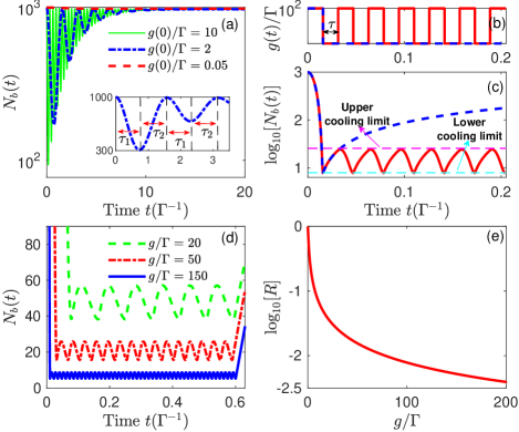
Figure 2: (color online) (a) Time evolution of mean phonon number $N_{b}(t)$ for $g/\Gamma=0.05,2,10$ where the inset shows the initial transient process of $N_{b}(t)$ for the case $g/\Gamma=2$. (b) shows the dynamical modulation of $g(t)$ and (c) describes the corresponding time evolution of $N_{b}(t)$, where blue dashed (red solid) curves denote the single pulse (periodic pulse) modulation. (d) Time evolution of $N_{b}(t)$ under pulsed modulation of the coupling strength with different intensities. (e) Brillouin cooling factor $R$ versus the coupling strength. Other parameters are $\gamma/\Gamma=0.01$, $\Delta_{1}/\Gamma=0.3$, $\Delta_{2}/\Gamma=3\times 10^{-5}$, and $n_{th}=1000$.

Breaking the steady-state cooling limit.—Although the strong optomechanical interaction does not significantly contribute to the steady-state cooling limit, it results in a Rabi oscillation for the phonon occupancy and thus leads the minimum phonon occupancy to be far smaller than the steady-state cooling limit, as shown in Fig. 2 (a). The system transfers from state $|n,m\rangle$ to state $|n,m-1\rangle$ by extracting phonons out of the acoustic field during the swapping-cooling-dominant time period ($\tau_{1}$). Analogously, it transfers from $|n,m\rangle$ to $|n,m+1\rangle$ by generating phonons during the swapping-heating-dominant time period ($\tau_{2}$). These two time periods alternate with a cycle $\tau_{1}=\tau_{2}=T/2$, as shown in the inset of Fig. 2 (a). To break the steady-state cooling limit and obtain a significant cooling rate, here we dynamically modulate the coupling strength $g(t)$ through a pulsed pump laser to permit the swapping cooling process and suppress the swapping heating process. We consider a short enough Brillouin-active waveguide, i.e., $L\ll\upsilon_{o}T/2$, where light fields will quickly pass through the waveguide and thus a pump laser can generate a coupling strength with pulsed-shape by switching on and off the pump. We switch on the pump laser during the swapping-cooling-dominant time period ($\tau_{1}$) to strengthen phonon absorption and switch off the pump during the swapping-heating-dominant time period ($\tau_{2}$) to halt the reversible Rabi oscillation and thus suppress the swapping heating process. We illustrate the modulation scheme of the pulsed coupling strength and the corresponding time evolution of the phonon occupancy in Figs. 2 (b) and (c), respectively. Since the phonon occupancy reaches the minimum value at the end of the first half Rabi oscillation, we switch off the pump abruptly at this time to prevent the energy from transferring back to phonons. During the pump switch-off time period, the phonons are only driven by the thermal environment, thus the phonon occupancy increases with the exponential growing rate $\Gamma/2$. After the optical fields passe through the waveguide, i.e., optical fields are initialized to the vacuum state, we switch on the pump laser to excite the swapping cooling process to absorb phonons and prevent the phonon occupancy from increasing continuously. By periodically modulating the coupling strength to initialize optical fields regularly, we can continuously suppress the swapping and thermal heating processes to keep a low phonon occupancy with a small-amplitude fluctuation and thus break the steady-state cooling limit, as shown by red solid curves in Figs. 2 (b) and (c). The instantaneous-state cooling limit, i.e., the lower cooling limit in Fig. 2 (c), can be approximately expressed as $N_{b}^{\rm{ins}}\approx\pi\Gamma n_{th}/(4g)$ which reduces the Brillouin steady-state cooling limit by a factor of $\pi\Gamma/(4g)$. The upper cooling limit in Fig. 2 (c) can be approximately expressed as $N_{b}^{\rm{upp}}\approx(1+\pi)\Gamma n_{th}/(4g)$. We know that in cavity optomechanical systems in the weak coupling regime, the cooling limit in the resolved-sideband regime is mainly dependent on the effective coupling strength $G$ and the optical dissipation rate $\gamma$ I-Wilson-Rae ; F-Marquardt ; C-Genes , i.e., $\sim n_{th}G^{2}/\gamma$. Here, as we consider the strong coupling regime and periodically evacuate the photons, the instantaneous-state cooling limit is decided by the ratio between the mechanical dissipation rate and the effective coupling strength.

In fact, the small-amplitude fluctuation around the instantaneous-state cooling limit is induced by the pulsed modulation of the coupling strength and the strong optomechanical interaction, which can be optimized by tuning the pump switch-off time $\tau$. In Fig. 2 (d), we show the time evolution of the phonon occupancy with periodical modulation of the coupling strength while the pump switch-off time is $\tau=0.05T$, where $g$ is the coupling strength during the pump switch-on time periods. We also present the Brillouin cooling factor $R$, which is the ratio of the instantaneous cooling limit to the initial phonon occupancy, in Fig. 2 (e). It indicates that a great Brillouin cooling factor, which reduces the steady-state cooling limit ($R\approx 1$) by several orders of magnitude, can be achieved through pulsed modulation of the optomechanical interaction, while photons experience lower damping than phonons. Moreover, this modulation scheme is switchable, i.e., the system will reach the instantaneous-state or steady-state cooling limits by turning on or off the modulation (see the Supplemental Material).

In addition, the above modulation scheme can also be applied to optomechanical cooling generated by forward anti-Stokes intermodal Brillouin scattering in continuous optomechanical systems Otterstrom , where lights experience higher damping than phonons. Actually, like the backward scattering case stated above, the phonon occupancy $\tilde{N}_{b}(t)$ corresponding to the forward intermodal Brillouin scattering exhibits a Rabi oscillation in the strong coupling regime, which enables lower phonon occupancy at some instantaneous states, as shown in Fig. 3 (a). Here, we choose the ratio between mechanical and optical dissipations according to the parameters measured in experiment Otterstrom . With a pulsed modulation of the optomechanical interaction to suppress heating processes, the phonon occupancy can be continuously maintained in a lower occupation with a small-amplitude fluctuation, which breaks the steady-state cooling limit, as shown in Fig. 3 (b).

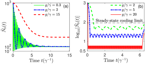
Figure 3: (color online) Dynamical Brillouin cooling via forward anti-Stokes intermodal scattering. (a) Time evolution of $\tilde{N}_{b}(t)$ for $g/\gamma=0.3,2,15$. (b) Dynamical cooling via pulsed modulation of the coupling intensity. Other parameters are $\Gamma/\gamma=0.1$, $\Delta_{1}/\gamma=0.05$, $\Delta_{2}/\gamma=5\times 10^{-6}$, and $n_{th}=1000$.

Conclusion.—We have shown that by periodically modulating the Brillouin interaction with a pulsed pump in the strong coupling regime, we can stimulate the swapping cooling process while suppressing the swapping heating process and thus obtain a significant Brillouin cooling factor with several orders of magnitude. It proves that cooling traveling-wave phonons into quantum ground state by utilizing backward Brillouin scattering is possible in continuous optomechanical systems while mechanical dissipation exceeds optical dissipation. Our scheme can also be applied to Brillouin cooling produced by forward intermodal Brillouin scattering and break the steady-state cooling limit. Moreover, this pulsed modulation scheme can be switchable. In addition, distinct from other pulsed cooling schemes that use complicated control methods Xiaoting ; Machnes or dynamic dissipative cooling by exploiting the optical dissipation Yongchun in cavity optomechanical systems, the simplicity and convenience of our method is achieved by simply controlling the pump pulse which makes the dynamic cooling scheme an effective experimental tool for quantum optomechanics. It should be pointed out that even though there is a small-amplitude fluctuation of the phonon occupancy around the instantaneous-state cooling limit, the Brillouin cooling limit can be viewed as stable in the sense of time averaging while the time scale is larger than the Rabi oscillation cycle $T$ Yongchun . This work opens the way for the exploration of quantum phenomena in continuous optomechanical systems through backward Brillouin scattering. The dynamical control of optomechanical interaction also provides a new way to study the quantum technologies, ranging from mechanical quantum states generation, quantum information processing, and high-precise measurement.

Appendix A Motion equation of linearized Brillouin interaction

The dynamics of the anti-Stokes Brillouin backward scattering in a typical waveguide can be given by

$$\frac{\partial a_{p}}{\partial t}+\upsilon_{o}\frac{\partial a_{p}}{\partial z} = -\frac{\gamma}{2}a_{p}-ig_{0}a_{as}b_{ac}^{\dagger}+\sqrt{\gamma}\xi_{p},$$

$$\frac{\partial a_{as}}{\partial t}-\upsilon_{o}\frac{\partial a_{as}}{\partial z} = -\frac{\gamma}{2}a_{as}-ig_{0}a_{p}b_{ac}+\sqrt{\gamma}\xi_{as},$$

$$\frac{\partial b_{ac}}{\partial t}-\upsilon_{b}\frac{\partial b_{ac}}{\partial z} = -\frac{\Gamma}{2}b_{ac}-ig_{0}a_{p}^{\dagger}a_{as}+\sqrt{\Gamma}\xi_{ac},$$ (4)

where $a_{p}$, $a_{as}$, and $b_{ac}$ denote the envelope operators of the pump field, anti-Stokes field, and acoustic field at their respective carrier frequencies $\omega_{p}$, $\omega_{as}$, and $\omega_{ac}$. $\upsilon_{o}$ and $\upsilon_{ac}$ represent the group velocities of the optical and acoustic fields. $\gamma$ and $\Gamma$ are the dissipation rates of the optical and acoustic fields. $g_{0}$ is the traveling-wave vacuum coupling rate which quantifies the interaction intensity between a single phonon and a single photonLaer1 . Without loss of generality, we take $g_{0}$ real and positive in our discussion. $\Delta_{1}=k\upsilon_{o}$ and $\Delta_{2}=k\upsilon_{ac}$ are the frequency shifts for the anti-Stokes photons and acoustic phonons which are induced by the wavenumber $k$, where $\Delta_{1}=\Delta_{2}=0$ corresponds to the case when the anti-Stokes optical mode and the acoustic mode are phase-matched with the pump mode. $\xi_{p}$, $\xi_{as}$, and $\xi_{ac}$ correspond to the Langevin noises of the pump field, anti-Stokes field, and acoustic field, which obey the following mean and correlation

$$\langle\xi_{p}(t,z)\rangle = 0,$$

$$\langle\xi_{as}(t,z)\rangle = 0,$$

$$\langle\xi_{ac}(t,z)\rangle = 0,$$

$$\langle\xi_{p}^{\dagger}(t_{1},z_{1})\xi_{p}(t_{2},z_{2})\rangle = 0,$$

$$\langle\xi_{as}^{\dagger}(t_{1},z_{1})\xi_{as}(t_{2},z_{2})\rangle = 0,$$

$$\langle\xi_{ac}^{\dagger}(t_{1},z_{1})\xi_{ac}(t_{2},z_{2})\rangle = n_{th}\delta(t_{1}-t_{2})\delta(z_{1}-z_{2}),$$

where $n_{th}=1/(e^{\hbar\omega_{ac}/k_{B}T_{m}}-1)$ is the thermal phonon occupation at the environment temperature $T_{m}$. By applying an undepleted pump field, the triply resonant optomechanical interaction can be reduced to a linearized optomechanical interaction between anti-Stokes field and acoustic field with a pump-enhanced coupling strength. Thus Eq. (A) can be reduced to

$$\frac{\partial a_{as}}{\partial t}-\upsilon_{o}\frac{\partial a_{as}}{\partial z} = -\frac{\gamma}{2}a_{as}-igb_{ac}+\sqrt{\gamma}\xi_{as},$$

$$\frac{\partial b_{ac}}{\partial t}-\upsilon_{ac}\frac{\partial b_{ac}}{\partial z} = -\frac{\Gamma}{2}b_{ac}-iga_{as}+\sqrt{\Gamma}\xi_{ac},$$ (6)

where $g=g_{0}\sqrt{\langle a_{p}^{\dagger}a_{p}\rangle}$ is the pump-enhanced spatial coupling rate. In fact, the phonon-mode and photon-mode $b_{ac}$ and $a_{as}$ are envelope operators with a continuous wavenumber and peaked around carrier wave vectors $k_{ac0}$ and $k_{as0}$, respectively, which can be expressed as Kharel ; Sipe

$$b_{ac} = \frac{1}{\sqrt{2\pi}}\int dkb_{k}e^{i(k-k_{ac0})z},$$

$$a_{as} = \frac{1}{\sqrt{2\pi}}\int dka_{k}e^{i(k-k_{as0})z},$$ (7)

where $b_{k}$ ($a_{k}$) denotes the annihilation operator for the $k$th phonon (photon) mode. Now we move to the momentum space by replacing $a_{as}$, $b_{ac}$, $\xi_{as}$, $\xi_{ac}$, and $\partial/\partial z$ with $a$, $b$, $\xi_{1}$, $\xi_{2}$, and $ik$ in Eq. (A) and obtain the motion equation of the linearized Brillouin interaction which can be given by

$$\frac{da(k,t)}{dt} = (-\frac{\gamma}{2}+i\Delta_{1})a-igb+\sqrt{\gamma}\xi_{1},$$

$$\frac{db(k,t)}{dt} = (-\frac{\Gamma}{2}+i\Delta_{2})b-iga+\sqrt{\Gamma}\xi_{2},$$ (8)

where the subscript $k$ of photon and phonon annihilation operators have been removed for simplification and $\xi_{1}$ ($\xi_{2}$) is the inverse Fourier transform of Langevin noise $\xi_{as}$ ($\xi_{ac}$). In order to derive the properties of Langevin noise $\xi_{1}(k,t)$, we decouple the optomechanical interaction between photons and phonons and assume that the anti-Stokes field $a(k,t)$ is driven by the Langevin noise $\xi_{1}(k,t)$, thus the quantum Langevin equation of $a(,t)$ can be given by

$$\dot{a}=(i\Delta_{1}-\frac{\gamma}{2})a+\sqrt{\gamma}\xi_{1},$$ (9)

where $\xi_{1}$ is a Gaussian random variable with zero mean, i.e., $\langle\xi_{1}(k,t)\rangle=0$, and $\delta$ correlation

$$\langle\xi_{1}^{\dagger}(k,t_{1})\xi_{1}(k,t_{2})\rangle=Q_{1}\delta(t_{1}-t_{2}).$$ (10)

The solution of Eq. (9) can be expressed as

$$a(k,t)=e^{(i\Delta_{1}-\gamma/2)t}\int_{-\infty}^{t}e^{-(i\Delta_{1}-\gamma/2)\tau}\sqrt{\gamma}\xi_{1}(k,\tau)d\tau.$$ (11)

Thus the equal-time correlation of $a$ can be expressed as

$$\langle a^{\dagger}(k,t)a(k,t)\rangle$$ (12)

$$= \gamma e^{-\gamma t}\int_{-\infty}^{t}e^{-(-i\Delta_{1}-\gamma/2)\tau_{1}}d\tau_{1}$$

$$\times\int_{-\infty}^{t}e^{-(i\Delta_{1}-\gamma/2)\tau_{2}}\langle\xi_{1}^{\dagger}(k,\tau_{1})\xi_{1}(k,\tau_{2})\rangle d\tau_{2}$$

$$= Q_{1}.$$

In addition, $\langle a^{\dagger}(k,t)a(k,t)$ corresponds to the thermal photon occupation $n_{th,o}$, i.e., $Q=n_{th,o}$. Hence, the correlation relation of Langevin noise $\xi_{1}$ can be given by

$$\langle\xi_{1}^{\dagger}(k,t_{1})\xi_{1}(k,t_{2})\rangle = n_{th,o}\delta(t_{1}-t_{2}),$$

$$\langle\xi_{1}(k,t_{1})\xi_{1}^{\dagger}(k,t_{1})\rangle = (1+n_{th,o})\delta(t_{1}-t_{2}).$$ (13)

Since the frequency of the anti-Stokes photons is high enough that the anti-Stokes field sits the quantum ground state, the thermal photon occupancy is zero, i.e., $n_{th,o}=0$. Therefore, the properties of Langevin noise $\xi_{1}$ can be expressed as

$$\langle\xi_{1}(k,t)\rangle = 0,$$

$$\langle\xi_{1}^{\dagger}(k,t_{1})\xi_{1}(k,t_{2})\rangle = 0,$$

$$\langle\xi_{1}(k,t_{1})\xi_{1}^{\dagger}(k,t_{1})\rangle = \delta(t_{1}-t_{2}).$$ (14)

Similarly, the properties of Langevin noise $\xi_{2}$ corresponding to the acoustic mode can be given by

$$\langle\xi_{2}(k,t)\rangle = 0,$$

$$\langle\xi_{2}^{\dagger}(k,t_{1})\xi_{2}(k,t_{2}) = n_{th}\delta(t_{1}-t_{2}),$$

$$\langle\xi_{2}(k,t_{1})\xi_{2}^{\dagger}(k,t_{2}) = (1+n_{th})\delta(t_{1}-t_{2}).$$ (15)

Appendix B Dynamics of mean phonon number in the strong coupling regime

Based on the motion equation of anti-Stokes photons and acoustic phonons described in Eq. (A), we have

$$\frac{d{a}^{\dagger}}{dt} = (-i\Delta_{1}-\frac{\gamma}{2})a^{\dagger}+igb^{\dagger}+\sqrt{\gamma}\xi_{1}^{\dagger},$$

$$\frac{d{b}^{\dagger}}{dt} = (-i\Delta_{2}-\frac{\Gamma}{2})b^{\dagger}+iga^{\dagger}+\sqrt{\Gamma}\xi_{2}^{\dagger}.$$ (16)

Combining with Eq. (A), these differential equations for the second-order moments $N_{a}=\langle a^{\dagger}a\rangle$, $N_{b}=\langle b^{\dagger}b\rangle$, $\langle a^{\dagger}b\rangle$ can be written as

$$\frac{dN_{a}}{dt} = -\gamma N_{a}-ig(\langle a^{\dagger}b\rangle-\langle a^{\dagger}b\rangle^{*})+\sqrt{\gamma}(\langle\xi_{1}^{\dagger}a\rangle+\langle\xi_{1}^{\dagger}a\rangle^{*}),$$

$$\frac{dN_{b}}{dt} = -\Gamma N_{b}+ig(\langle a^{\dagger}b\rangle-\langle a^{\dagger}b\rangle^{*})+\sqrt{\Gamma}(\langle\xi^{\dagger}_{2}b\rangle+\langle\xi^{\dagger}_{2}b\rangle^{*}),$$

$$\frac{d\langle a^{\dagger}b\rangle}{dt} = -\left(i(\Delta_{1}-\Delta_{2})+\frac{\gamma+\Gamma}{2}\right)\langle a^{\dagger}b\rangle-igN_{a}+igN_{b}$$ (17)

$$+\sqrt{\gamma}\langle\xi_{1}^{\dagger}b\rangle+\sqrt{\Gamma}\langle a^{\dagger}\xi_{2}\rangle,$$

where $N_{a}$ and $N_{b}$ denote the mean photon and phonon numbers, respectively. In order to evaluate the noise-related terms in Eq. (B), we apply the following Fourier transform

$$\bar{a}(\omega) = \int_{-\infty}^{\infty}a(t)e^{i\omega t}dt,$$

$$\bar{b}(\omega) = \int_{-\infty}^{\infty}b(t)e^{i\omega t}dt,$$

$$\bar{\xi}_{1}(\omega) = \int_{-\infty}^{\infty}\xi_{1}(t)e^{i\omega t}dt,$$

$$\bar{\xi}_{2}(\omega) = \int_{-\infty}^{\infty}\xi_{2}(t)e^{i\omega t}dt,$$ (18)

to Eq. (A) and obtain

$$-i\omega\bar{a} = (i\Delta_{1}-\frac{\gamma}{2})\bar{a}-ig\bar{b}+\sqrt{\gamma}\bar{\xi}_{1},$$

$$-i\omega\bar{b} = (i\Delta_{2}-\frac{\Gamma}{2})\bar{b}-ig\bar{a}+\sqrt{\Gamma}\bar{\xi}_{2},$$ (19)

where the correlation relations of noises $\bar{\xi}_{1,2}$ can be calculated based on the correlation functions described in Eqs. (A) and (A) and given by

$$\langle\bar{\xi}_{1}^{\dagger}(\omega_{1})\bar{\xi}_{1}(\omega_{2})\rangle = 0,$$

$$\langle\bar{\xi}_{2}^{\dagger}(\omega_{1})\bar{\xi}_{2}(\omega_{2})\rangle = 2\pi n_{th}\delta(\omega_{1}-\omega_{2}),$$

$$\langle\bar{\xi}_{1}^{\dagger}(\omega_{1})\bar{\xi}_{2}(\omega_{2})\rangle = 0,$$

$$\langle\bar{\xi}_{1}(\omega_{1})\bar{\xi}_{2}^{\dagger}(\omega_{2})\rangle = 0.$$ (20)

The solution of $\bar{a}(\omega),\bar{b}(\omega)$ can be expressed as

$$\bar{a}(\omega) = -\frac{\left(i(\omega+\Delta_{2})-\frac{\Gamma}{2}\right)\sqrt{\gamma}\bar{\xi}_{1}(\omega)+ig\sqrt{\Gamma}\bar{\xi}_{2}(\omega)}{\Xi},$$

$$\bar{b}(\omega) = -\frac{ig\sqrt{\gamma}\bar{\xi}_{1}(\omega)+\left(i(\omega+\Delta_{1})-\frac{\gamma}{2}\right)\sqrt{\Gamma}\bar{\xi}_{2}(\omega)}{\Xi},$$

with

$$\Xi = g^{2}+\frac{\gamma\Gamma}{4}-(\omega+\Delta_{1})(\omega+\Delta_{2})$$ (22)

$$-i\left(\frac{\gamma}{2}(\omega+\Delta_{2})+\frac{\Gamma}{2}(\omega+\Delta_{1})\right).$$

By substituting Eqs. (B) and (B) into $\langle\xi_{1}^{\dagger}(t)a(t)\rangle$, we have

$$\langle\xi_{1}^{\dagger}(t)a(t)\rangle$$ (23)

$$= \frac{1}{4\pi^{2}}\int_{-\infty}^{\infty}e^{i\omega_{1}t}d\omega_{1}\int_{-\infty}^{\infty}e^{-i\omega_{2}t}\langle\bar{\xi}_{1}^{\dagger}(\omega_{1})\bar{a}(\omega_{2})\rangle d\omega_{2}$$

$$= -\frac{1}{4\pi^{2}}\int_{-\infty}^{\infty}e^{i\omega_{1}t}d\omega_{1}\int_{-\infty}^{\infty}e^{-i\omega_{2}t}\times$$

$$\langle\bar{\xi}_{1}^{\dagger}(\omega_{1})\frac{\left(i(\omega_{2}+\Delta_{2})-\frac{\Gamma}{2}\right)\sqrt{\gamma}\bar{\xi}_{1}(\omega_{2})+ig\sqrt{\Gamma}\bar{\xi}_{2}(\omega_{2})}{\Xi}\rangle d\omega_{2}$$

$$= 0.$$

Similarly, $\langle\xi_{2}^{\dagger}b\rangle$, $\langle\xi_{1}^{\dagger}b\rangle$, and $\langle a^{\dagger}\xi_{2}\rangle$ can be calculated as follows

$$\langle\xi^{\dagger}_{2}(t)b(t)\rangle$$ (24)

$$= \frac{1}{4\pi^{2}}\int_{-\infty}^{\infty}e^{i\omega_{1}t}d\omega_{1}\int_{-\infty}^{\infty}e^{-i\omega_{2}t}\langle\bar{\xi}_{2}^{\dagger}(\omega_{1})\bar{b}(\omega_{2})\rangle d\omega_{2}$$

$$= -\frac{\sqrt{\Gamma}n_{th}}{2\pi}\int_{-\infty}^{\infty}\frac{i(\omega+\Delta_{1})-\frac{\gamma}{2}}{\Xi}d\omega,$$

$$\langle\xi_{1}^{\dagger}(t)b(t)\rangle$$ (25)

$$= \frac{1}{4\pi^{2}}\int_{-\infty}^{\infty}e^{i\omega_{1}t}d\omega_{1}\int_{-\infty}^{\infty}e^{-i\omega_{2}t}\langle\bar{\xi}_{1}^{\dagger}(\omega_{1})\bar{b}(\omega_{2})\rangle d\omega_{2}$$

$$= 0,$$

and

$$\langle a^{\dagger}(t)\xi_{2}(t)\rangle$$ (26)

$$= \frac{1}{4\pi^{2}}\int_{-\infty}^{\infty}e^{i\omega_{1}t}d\omega_{1}\int_{-\infty}^{\infty}e^{-i\omega_{2}t}\langle\bar{a}^{\dagger}(\omega_{1})\bar{\xi}_{2}(\omega_{2})\rangle d\omega_{2}$$

$$= \frac{ign_{th}\sqrt{\Gamma}}{2\pi}\int_{-\infty}^{\infty}\frac{1}{\Xi}d\omega.$$

Hence, the noise-related terms in Eq. (B) can be expressed as follows

$$\langle\xi_{1}^{\dagger}a\rangle+\langle\xi_{1}^{\dagger}a\rangle^{*} = 0,$$ (27)

$$\langle\xi_{2}^{\dagger}b\rangle+\langle\xi_{2}^{\dagger}b\rangle^{*} = \frac{\sqrt{\Gamma}n_{th}}{2\pi}\int_{-\infty}^{\infty}$$

$$\frac{\gamma(g^{2}+\frac{\gamma\Gamma}{4})+\Gamma(\omega+\Delta_{1})^{2}}{\Lambda_{1}}d\omega,$$

$$\sqrt{\gamma}\langle\xi_{1}^{\dagger}b\rangle+\sqrt{\Gamma}\langle a^{\dagger}\xi_{2}\rangle = \frac{ign_{th}\Gamma}{2\pi}\int_{-\infty}^{\infty}\frac{1}{\Lambda_{2}}d\omega,$$ (29)

with

$$\Lambda_{1} = \left(g^{2}+\frac{\gamma\Gamma}{4}-(\omega^{2}+(\Delta_{1}+\Delta_{2})\omega+\Delta_{1}\Delta_{2}\right)^{2}$$

$$+\left(\frac{\gamma+\Gamma}{2}\omega+\frac{\gamma\Delta_{2}+\Gamma\Delta_{1}}{2}\right)^{2},$$

$$\Lambda_{2} = g^{2}+\frac{\gamma\Gamma}{4}-(\omega+\Delta_{1})(\omega+\Delta_{2})$$ (30)

$$+i\left(\frac{\gamma}{2}(\omega+\Delta_{2})+\frac{\Gamma}{2}(\omega+\Delta_{1})\right).$$

Here, we consider the strong coupling regime, i.e., $g\gg\Gamma,\gamma$. Furthermore, for the backward Brillouin scattering in a typical Brillouin-active waveguide, the mechanical dissipation is far larger than the optical dissipation ($\Gamma\gg\gamma$) and the optical group velocity is significantly faster than the mechanical group velocity ($\upsilon_{o}\gg\upsilon_{ac}$, i.e., $\Delta_{1}\gg\Delta_{2}$). We also consider that the wavenumber induced frequency shifts are within the linewidth of the acoustic mode ($\Delta_{1,2}<\Gamma$). Thus $\langle\xi_{2}^{\dagger}b\rangle+\langle\xi_{2}^{\dagger}b\rangle^{*}$ can be approximated as follows

$$\langle\xi_{2}^{\dagger}(t)b(t)\rangle+\langle\xi_{2}^{\dagger}(t)b(t)\rangle^{*}$$ (31)

$$\approx \frac{\sqrt{\Gamma}n_{th}}{2\pi}\int_{-\infty}^{\infty}\frac{\gamma(g^{2}+\frac{\gamma\Gamma}{4})+\Gamma\omega^{2}}{\left(g^{2}+\frac{\gamma\Gamma}{4}+\Delta_{1}\omega-\omega^{2}\right)^{2}+\left(\frac{\gamma+\Gamma}{2}\right)^{2}\omega^{2}}d\omega$$

$$\approx \frac{\sqrt{\Gamma}n_{th}}{2\pi}\int_{-\infty}^{\infty}\frac{\gamma\alpha^{2}+\Gamma\omega^{2}}{(\alpha^{2}+\Delta_{1}\omega-\omega^{2})^{2}+\beta^{2}\omega^{2}}d\omega,$$

where

$$\alpha=\sqrt{g^{2}+\frac{\gamma\Gamma}{4}},\quad\beta=\frac{\gamma+\Gamma}{2}.$$ (32)

Eq. (31) can be further calculated as follows

$$\frac{\sqrt{\Gamma}n_{th}}{2\pi}\int_{-\infty}^{\infty}\frac{\gamma\alpha^{2}+\Gamma\omega^{2}}{(\alpha^{2}+\Delta_{1}\omega-\omega^{2})^{2}+\beta^{2}\omega^{2}}d\omega$$

$$= \frac{\sqrt{\Gamma}n_{th}}{2\pi}\int_{-\infty}^{\infty}\frac{1}{\alpha^{2}}\frac{\gamma+\Gamma\left(\frac{\omega}{\alpha}\right)^{2}}{\left(1+\frac{\Delta_{1}}{\alpha}\frac{\omega}{\alpha}-\left(\frac{\omega}{\alpha}\right)^{2}\right)^{2}+\frac{\beta^{2}}{\alpha^{2}}\left(\frac{\omega}{\alpha}\right)^{2}}d\omega$$

$$= \frac{\sqrt{\Gamma}n_{th}}{2\pi\alpha}\int_{-\infty}^{\infty}\frac{\gamma+\Gamma\omega^{2}}{\left(1+\frac{\Delta_{1}}{\alpha}\omega-\omega^{2}\right)^{2}+\frac{\beta^{2}}{\alpha^{2}}\omega^{2}}d\omega$$

$$= \frac{\sqrt{\Gamma}n_{th}}{2\pi\alpha}\int_{-\infty}^{\infty}\frac{\gamma+\Gamma\omega^{2}}{\omega^{4}-2\eta_{2}\omega^{3}+(\eta_{2}^{2}-2\eta_{1})\omega^{2}+2\eta_{2}\omega+1}d\omega$$

$$= \frac{\sqrt{\Gamma}n_{th}}{2\pi\alpha}\int_{-\infty}^{\infty}\frac{A_{1}}{\omega-\lambda_{1}}+\frac{A_{2}}{\omega-\lambda_{2}}+\frac{A_{3}}{\omega-\lambda_{3}}+\frac{A_{4}}{\omega-\lambda_{4}}d\omega$$

where

$$\eta_{1}=1-\frac{\beta^{2}}{2\alpha^{2}},\quad\eta_{2}=\frac{\Delta_{1}}{\alpha},$$ (34)

$$\lambda_{1} = -i\sqrt{\frac{1-\eta_{1}}{2}}+\frac{\eta_{2}}{2}-\sqrt{\frac{1+\eta_{1}}{2}+\frac{\eta_{2}^{2}}{4}-i\eta_{2}\sqrt{\frac{1-\eta_{1}}{2}}},$$

$$\lambda_{2} = -i\sqrt{\frac{1-\eta_{1}}{2}}+\frac{\eta_{2}}{2}+\sqrt{\frac{1+\eta_{1}}{2}+\frac{\eta_{2}^{2}}{4}-i\eta_{2}\sqrt{\frac{1-\eta_{1}}{2}}},$$

$$\lambda_{3} = i\sqrt{\frac{1-\eta_{1}}{2}}+\frac{\eta_{2}}{2}-\sqrt{\frac{1+\eta_{1}}{2}+\frac{\eta_{2}^{2}}{4}+i\eta_{2}\sqrt{\frac{1-\eta_{1}}{2}}},$$

$$\lambda_{4} = i\sqrt{\frac{1-\eta_{1}}{2}}+\frac{\eta_{2}}{2}+\sqrt{\frac{1+\eta_{1}}{2}+\frac{\eta_{2}^{2}}{4}+i\eta_{2}\sqrt{\frac{1-\eta_{1}}{2}}},$$

and

$$A_{1} = \frac{\gamma+\Gamma\lambda_{1}^{2}}{(\lambda_{1}-\lambda_{2})(\lambda_{1}-\lambda_{3})(\lambda_{1}-\lambda_{4})},$$

$$A_{2} = -\frac{\gamma+\Gamma\lambda_{2}^{2}}{(\lambda_{1}-\lambda_{2})(\lambda_{2}-\lambda_{3})(\lambda_{2}-\lambda_{4})},$$

$$A_{3} = \frac{\gamma+\Gamma\lambda_{3}^{2}}{(\lambda_{1}-\lambda_{3})(\lambda_{2}-\lambda_{3})(\lambda_{3}-\lambda_{4})},$$

$$A_{4} = -\frac{\gamma+\Gamma\lambda_{4}^{2}}{(\lambda_{1}-\lambda_{4})(\lambda_{2}-\lambda_{4})(\lambda_{3}-\lambda_{4})}.$$ (36)

These eigenvalues described in Eq. (B) can be rewritten as

$$\lambda_{1} = \frac{\eta_{2}}{2}-\sqrt{A}\cos\frac{\theta}{2}+i\left(\sqrt{A}\sin\frac{\theta}{2}-\sqrt{\frac{1-\eta_{1}}{2}}\right),$$

$$\lambda_{2} = \frac{\eta_{2}}{2}+\sqrt{A}\cos\frac{\theta}{2}-i\left(\sqrt{A}\sin\frac{\theta}{2}+\sqrt{\frac{1-\eta_{1}}{2}}\right),$$

$$\lambda_{3} = \frac{\eta_{2}}{2}-\sqrt{A}\cos\frac{\theta}{2}-i\left(\sqrt{A}\sin\frac{\theta}{2}-\sqrt{\frac{1-\eta_{1}}{2}}\right),$$

$$\lambda_{4} = \frac{\eta_{2}}{2}+\sqrt{A}\cos\frac{\theta}{2}+i\left(\sqrt{A}\sin\frac{\theta}{2}+\sqrt{\frac{1-\eta_{1}}{2}}\right).$$

As $g\gg\Gamma\gg\gamma$ and $\Gamma>\Delta_{1}$, the above eigenvalues can be approximated to

$$\lambda_{1} \approx -\sqrt{A}\cos\frac{\theta}{2}-i\sqrt{\frac{1-\eta_{1}}{2}},$$

$$\lambda_{2} \approx \sqrt{A}\cos\frac{\theta}{2}-i\sqrt{\frac{1-\eta_{1}}{2}},$$

$$\ \lambda_{3} \approx -\sqrt{A}\cos\frac{\theta}{2}+i\sqrt{\frac{1-\eta_{1}}{2}},$$

$$\lambda_{4} \approx \sqrt{A}\cos\frac{\theta}{2}+i\sqrt{\frac{1-\eta_{1}}{2}}.$$ (38)

Substituting Eq. (B) into Eq. (B), we have

$$\frac{\sqrt{\Gamma}n_{th}}{2\pi}\int_{-\infty}^{\infty}\frac{\gamma\alpha^{2}+\Gamma\omega^{2}}{(\alpha^{2}+\Delta_{1}\omega-\omega^{2})^{2}+\beta^{2}\omega^{2}}d\omega$$ (39)

$$= \frac{\sqrt{\Gamma}n_{th}}{2\pi\alpha}\int_{-\infty}^{\infty}\frac{A_{1}}{\omega-\lambda_{1}}+\frac{A_{2}}{\omega-\lambda_{2}}+\frac{A_{3}}{\omega-\lambda_{3}}+\frac{A_{4}}{\omega-\lambda_{4}}d\omega$$

$$= \frac{\sqrt{\Gamma}n_{th}}{2\pi\alpha}i\pi(-A_{1}-A_{2}+A_{3}+A_{4})$$

$$= \sqrt{\Gamma}n_{th},$$

i.e.,

$$\langle\xi_{2}^{\dagger}(t)b(t)\rangle+\langle\xi_{2}^{\dagger}(t)b(t)\rangle^{*}\approx\sqrt{\Gamma}n_{th}.$$ (40)

Similarly, the equal-time correlation $\sqrt{\gamma}\langle\xi_{1}^{\dagger}b\rangle+\sqrt{\Gamma}\langle a^{\dagger}\xi_{2}\rangle$ (Eq. (29)) can be calculated as follows

$$\sqrt{\gamma}\langle\xi_{1}^{\dagger}(t)b(t)\rangle+\sqrt{\Gamma}\langle a^{\dagger}(t)\xi_{2}(t)\rangle$$ (41)

$$\approx \frac{gn_{th}\Gamma}{2\pi}\int_{-\infty}^{\infty}\frac{\frac{\gamma+\Gamma}{2}\omega}{\left(g^{2}+\frac{\gamma\Gamma}{4}+\Delta_{1}\omega-\omega^{2}\right)^{2}+\left(\frac{\gamma+\Gamma}{2}\right)^{2}\omega^{2}}d\omega$$

$$+i\frac{gn_{th}\Gamma}{2\pi}\int_{-\infty}^{\infty}\frac{g^{2}+\frac{\gamma\Gamma}{4}+\Delta_{1}\omega-\omega^{2}}{\left(g^{2}+\frac{\gamma\Gamma}{4}+\Delta_{1}\omega-\omega^{2}\right)^{2}+\left(\frac{\gamma+\Gamma}{2}\right)^{2}\omega^{2}}d\omega$$

$$\approx -\frac{gn_{th}\Gamma\beta}{4\alpha^{2}}\times$$

$$\frac{2A\sin\theta-\sqrt{2(1-\eta_{1})}\eta_{2}}{1+\eta_{1}^{2}-\frac{A^{2}}{2}+2A\cos\theta+\frac{A^{2}}{2}\cos 2\theta-2\eta_{1}(1+A\cos\theta)}$$

$$-i\frac{gn_{th}\Gamma}{4\alpha}\times$$

$$\frac{\sqrt{2(1-\eta_{1})}(-1+2A\cos\theta-\eta_{1}+\frac{\eta_{2}^{2}}{2})-2A\eta_{2}\sin\theta}{1+\eta_{1}^{2}-\frac{A^{2}}{2}+2A\cos\theta+\frac{A^{2}}{2}\cos 2\theta-2\eta_{1}(1+A\cos\theta)}$$

$$\approx 0.$$

Finally, by substituting Eqs. (27), (40) and (41) into Eq. (B), the dynamics of the mean photon number $N_{a}$ and mean phonon number $N_{b}$ can be given by

$$\frac{dN_{a}}{dt} = -\gamma N_{a}-ig(\langle a^{\dagger}b\rangle-\langle a^{\dagger}b\rangle^{*}),$$

$$\frac{dN_{b}}{dt} = -\Gamma N_{b}+ig(\langle a^{\dagger}b\rangle-\langle a^{\dagger}b\rangle^{*})+\Gamma n_{th},$$

$$\frac{d\langle a^{\dagger}b\rangle}{dt} = -\left(i(\Delta_{1}-\Delta_{2})+\frac{\gamma+\Gamma}{2}\right)\langle a^{\dagger}b\rangle-igN_{a}+igN_{b},$$

and the analytical solution of mean phonon number $N_{b}(t)$ can be expressed as

$$N_{b}(t) = C_{1}e^{-\left(\frac{\gamma+\Gamma}{2}+\Gamma_{0}\right)t}+C_{2}e^{-\left(\frac{\gamma+\Gamma}{2}-\Gamma_{0}\right)t}$$

$$+C_{3}e^{-\frac{\gamma+\Gamma}{2}t}\cos(\Omega t)+C_{4}e^{-\frac{\gamma+\Gamma}{2}t}\sin(\Omega t)+N_{b}^{ss},$$

where

$$\Omega = \frac{1}{2}\sqrt{\sqrt{\Upsilon}+\left(8g^{2}+2\Delta_{1}^{2}-\frac{1}{2}(\Gamma-\gamma)^{2}\right)},$$ (44)

$$\Gamma_{0} = \frac{1}{2}\sqrt{\sqrt{\Upsilon}-\left(8g^{2}+2\Delta_{1}^{2}-\frac{1}{2}(\Gamma-\gamma)^{2}\right)},$$ (45)

$$N_{b}^{ss} = \frac{4g^{2}(\Gamma+\gamma)+\gamma(\Gamma+\gamma)^{2}+4\gamma\Delta_{1}^{2}}{4g^{2}(\Gamma+\gamma)+\gamma\Gamma(\Gamma+\gamma)+4\gamma\Gamma\Delta_{1}^{2}/(\Gamma+\gamma)}\cdot\frac{\Gamma}{\Gamma+\gamma}n_{th},$$

with

$$\Upsilon=\left(8g^{2}+2\Delta_{1}^{2}-\frac{1}{2}(\Gamma-\gamma)^{2}\right)^{2}+4(\Gamma-\gamma)^{2}\Delta_{1}^{2}.$$ (47)

and the coefficients $C_{i}$ can be given by

$$C_{1} = -\frac{-16g^{2}\gamma+(\Gamma+\gamma)\left((\Gamma+\gamma)^{2}+4\Omega^{2}\right)}{16\Gamma_{0}(\Omega^{2}+\Gamma_{0}^{2})}n_{th}$$

$$-\frac{+2\left(8g^{2}-(\Gamma+\gamma)^{2}-4\Omega^{2}\right)\Gamma_{0}}{16\Gamma_{0}(\Omega^{2}+\Gamma_{0}^{2})}n_{th}$$

$$+\frac{\left((\Gamma+\gamma)^{2}+4\Omega^{2}\right)(\Gamma+\gamma-2\Gamma_{0})}{16\Gamma_{0}(\Omega^{2}+\Gamma_{0}^{2})}N_{b}^{ss},$$

$$C_{2} = -\frac{16g^{2}\gamma-(\Gamma+\gamma)\left((\Gamma+\gamma)^{2}+4\Omega^{2}\right)}{16\Gamma_{0}(\Omega^{2}+\Gamma_{0}^{2})}n_{th}$$

$$-\frac{+2\left(8g^{2}-(\Gamma+\gamma)^{2}-4\Omega^{2}\right)\Gamma_{0}}{16\Gamma_{0}(\Omega^{2}+\Gamma_{0}^{2})}n_{th}$$

$$-\frac{\left((\Gamma+\gamma)^{2}+4\Omega^{2}\right)(\Gamma+\gamma+2\Gamma_{0})}{16\Gamma_{0}(\Omega^{2}+\Gamma_{0}^{2})}N_{b}^{ss},$$

$$C_{3} = \frac{8g^{2}+4\Gamma_{0}^{2}-(\Gamma+\gamma)^{2}}{4(\Omega^{2}+\Gamma_{0}^{2})}n_{th}+\frac{(\Gamma+\gamma)^{2}-4\Gamma_{0}^{2}}{4(\Omega^{2}+\Gamma_{0}^{2})}N_{b}^{ss}$$

$$C_{4} = \frac{16g^{2}\gamma+4(\Gamma+\gamma)\Gamma_{0}^{2}-(\Gamma+\gamma)^{3}}{8\Omega(\Omega^{2}+\Gamma_{0}^{2})}n_{th}$$ (48)

$$+\frac{(\Gamma+\gamma)^{2}-4\Gamma_{0}^{2}}{8\Omega(\Omega^{2}+\Gamma_{0}^{2})}(\Gamma+\gamma)N_{b}^{ss}.$$

$\Omega$ is the Rabi oscillation frequency induced by the strong optomechanical interaction and $N_{b}^{ss}$ is the steady-state cooling limit. Here, we assume that the initial states of the Stokes field and acoustic field are vacuum state and thermal state, respectively, i.e., $N_{a}(t=0)=0,N_{b}(t=0)=n_{th}$. Eq. (B) can be approximated to

$$N_{b}(t) \approx \tilde{C}_{1}e^{-\frac{\Gamma+\gamma}{2}t}+\tilde{C}_{2}e^{-\frac{\Gamma+\gamma}{2}t}\cos(\Omega t)+\tilde{C}_{3}e^{-\frac{\Gamma+\gamma}{2}t}\sin(\Omega t)$$ (49)

$$+\frac{\Gamma}{\Gamma+\gamma}n_{th},$$

where

$$\Omega \approx \sqrt{4g^{2}+\Delta_{1}^{2}-\frac{(\Gamma-\gamma)^{2}}{4}},$$

$$\tilde{C}_{1} \approx -\frac{2(\Gamma-\gamma)g^{2}-\gamma(\Delta_{1}^{2}+\gamma\Gamma)}{(\Gamma+\gamma)\Omega^{2}}n_{th},$$

$$\tilde{C}_{2} \approx \frac{2g^{2}-\gamma(\Gamma+\gamma)/4}{\Omega^{2}}n_{th},$$

$$\tilde{C}_{3} \approx \frac{\gamma g-\gamma(\Gamma+\gamma)^{2}/(16g)}{\Omega^{2}}n_{th}.$$ (50)

We show the time evolution of mean phonon number $N_{b}(t)$ under strong coupling condition in Figs. 4 (a) and (b) where blue solid and red dashed curves correspond to the simulation results and analytical solution described in Eq. (49), respectively.

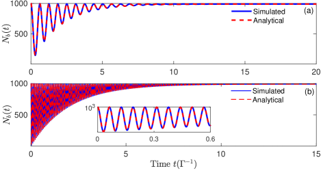
Figure 4: (Color online) Time evolution of phonon occupancy $N_{b}(t)$ in the strong coupling regime for $g/\Gamma=5$ (a) and $g/\Gamma=50$ (b). The blue solid curves represent simulated results and the red dashed curves correspond to the analytical expression described in Eq. (49). The inset in (b) shows the initial transient process of $N_{b}(t)$ for $g/\Gamma=50$. Other parameters are $\gamma/\Gamma=0.01$, $\Delta_{1}/\Gamma=0.3$, $\Delta_{2}/\Gamma=3\times 10^{-5}$, and $n_{th}=1000$.

Appendix C Dynamical cooling via pulsed modulation of optomechanical coupling

In the main text we have mentioned that there exists a state swapping with cycle $T$ between anti-Stokes photons and acoustic phonons in the strong coupling regime, which includes the swapping cooling and heating processes. We switch on the Brillouin interaction during the swapping cooling dominated time period to strengthen the energy transfer from phonons to anti-Stokes photons. When the phonon occupancy reaches the minimal value, we switch off the Brillouin interaction to suppress the swapping heating process, i.e., preventing the energy from transferring back to the anti-Stokes photons. During the switch-off time period, the acoustic mode is individually driven by the thermal environment. After the light fields pass through the waveguide and be initialized to the vacuum state, we switch on the Brillouin interaction again to extract the phonons out of the acoustic field. By modulating

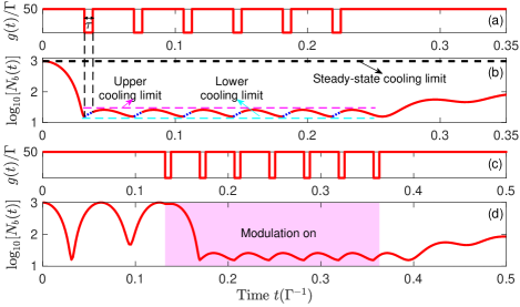
Figure 5: (Color online) Pulsed modulation scheme of coupling strength $g(t)$ and corresponding time evolution of phonon occupancy $N_{b}(t)$. (a) and (b) correspond to the case where the modulation begins at time $T/2$. The blue dashed curves in (b) describe the dynamics of phonon occupancy during the pump switch-off time periods while the switch-off time $\tau=0.1T$. (c) and (d) correspond to the case where the modulation starts at time $2.1T$.

the optomechanical coupling strength to periodically initialize the optical fields, we can continuously enhance the swapping cooling process while suppress the swapping heating process and keep the phonon occupation in an instantaneously-state cooling limit with a small-amplitude fluctuation. This periodical modulation of the coupling strength can be achieved by a pulsed pump when the Brillouin-active waveguide is short enough ($L\ll\upsilon_{o}T/2$). We illustrate the pulsed modulation scheme of the coupling strength and the corresponding time evolution of the phonon occupancy $N_{b}(t)$ in Figs. 5 (a) and (b), respectively, where $\tau$ represents the switch-off time of pump field. Here, we start the modulation at the end of the first half Rabi oscillation cycle $t=T/2$ since the minimum value of $N_{b}(t)$ is achieved at this time. By substituting $t=T/2=\pi/\Omega$ into Eq. (49), we calculate the instantaneous-state cooling limit $N_{b}^{\rm{ins}}$, i.e., the lower cooling limit (red dashed curve) in Fig. 5 (b), as follows

$$N_{b}^{\rm{ins}} = N_{b}(t=\frac{\pi}{\Omega})$$ (51)

$$\approx \tilde{C}_{1}e^{-\frac{(\Gamma+\gamma)\pi}{2\Omega}}+\tilde{C}_{2}e^{-\frac{(\Gamma+\gamma)\pi}{2\Omega}}\cos(\pi)$$

$$+\tilde{C}_{3}e^{-\frac{(\Gamma+\gamma)\pi}{2\Omega}}\sin(\pi)+\frac{\Gamma}{\Gamma+\gamma}n_{th}$$

$$\approx \frac{\pi(\Gamma+\gamma)g+\Delta_{1}^{2}-\frac{(\Gamma-\gamma)^{2}}{4}}{4g^{2}+\Delta_{1}^{2}-\frac{(\Gamma-\gamma)^{2}}{4}}\cdot\frac{\Gamma}{\Gamma+\gamma}n_{th}$$

$$\approx \frac{\pi\Gamma}{4g}n_{th}.$$

In order to evaluate the upper cooling limit $N_{b}^{\rm{upp}}$, we assume that the pump switch-off time $\tau$ is small enough that the increase of the phonon occupancy during the switch-off time can be omitted. Therefore, the analytical expression of phonon occupancy $N_{b}(t)$ during time period $[0,\ T/2]$ can be described by Eq. (49) and during time period $[T/2,\ T]$ can be approximately given by

$$N_{b}(t) \approx \bar{C}_{1}e^{-\frac{\Gamma+\gamma}{2}(t-\frac{T}{2})}+\bar{C}_{2}e^{-\frac{\Gamma+\gamma}{2}(t-\frac{T}{2})}\cos(\Omega t)$$ (52)

$$+\bar{C}_{3}e^{-\frac{\Gamma+\gamma}{2}(t-\frac{T}{2})}\sin(\Omega t)+\frac{\Gamma}{\Gamma+\gamma}n_{th},$$

where

$$\bar{C}_{1} \approx \frac{-8g^{2}+\pi(\gamma+\Gamma)g}{2\Omega^{2}}\cdot\frac{\Gamma}{\Gamma+\gamma}n_{th},$$

$$\bar{C}_{2} \approx -\frac{2\pi(\gamma+\Gamma)g+\Gamma(\Gamma-2\gamma)}{4\Omega^{2}}\cdot\frac{\Gamma}{\Gamma+\gamma}n_{th},$$

$$\bar{C}_{3} \approx -\frac{4g-\pi(\Gamma-\gamma)}{4\Omega^{2}}\cdot\Gamma n_{th},$$

$$\Omega \approx \sqrt{4g^{2}+\Delta_{1}^{2}-(\Gamma-\gamma)^{2}/4}.$$ (53)

We calculate $N_{b}(t)$ at time $t=3T/4$ to approximately evaluate $N_{b}^{\rm{upp}}$, i.e.,

$$N_{b}^{\rm{upp}} \approx \bar{C}_{1}e^{-\frac{\Gamma+\gamma}{2}\frac{\pi}{2\Omega}}+\bar{C}_{2}e^{-\frac{\Gamma+\gamma}{2}\frac{\pi}{2\Omega}}\cos\frac{3\pi}{2}$$ (54)

$$+\bar{C}_{3}e^{-\frac{\Gamma+\gamma}{2}\frac{\pi}{2\Omega}}\sin\frac{3\pi}{2}+\frac{\Gamma}{\Gamma+\gamma}n_{th}$$

$$\approx \frac{(1+\pi)\Gamma}{4g}n_{th}.$$

In Fig. 5 (b), we apply the modulation of the coupling strength at the end of first half Rabi oscillation cycle since the phonon occupancy reaches the minimum value at this time. Actually, we can turn on the modulation at any time to cool the phonons. We show the time evolution of the phonon occupancy while the modulation is turned on at time $t=2.1T$ in Fig. 5 (d), where Fig. 5 (c) denotes the modulation scheme. The acoustic mode reaches the instantaneous-state cooling limit when the modulation is turned on and transits back to the steady-state cooling limit while the modulation is turned off. It means that this dynamic cooling scheme with pulsed modulation of the optomechanical coupling intensity is switchable, as shown in Fig. 6.

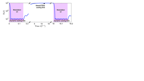
Figure 6: (Color online) The pulsed modulation of the coupling strength is switchable where the regions with light purple color correspond to the modulation turned on.

Appendix D Continuum optomechanical cooling via Brillouin interaction

In cavity optomechanical systems, as the optical and the mechanical modes which cause the optomechanical interaction are discrete modes, the sideband cooling method can only generate a net cooling effect on a single mechanical mode Teufel2 ; Chan . However, in continuum optomechanical systems, for example, Brillouin-active waveguides, the optomechanical interaction involves the acoustic field with a continuous band of accessible modes, which enables the continuum optomechanical cooling Otterstrom ; Chen . In fact, as described in Eq. (A), the envelope operator $b_{ac}$ of the acoustic filed associated in the Brillouin interaction is an operator with continuous wavenumber $k$, which is peaked around a carrier wave vector $k_{ac0}$ and enables the acoustic field to evolve in space. Thus, in the momentum space, if we consider an undepleted pump, we can obtain motion equations as described in Eq. (A) for each specific wavenumber $k$ and then achieve the dynamics of the mean phonon number $N_{b}(k,t)=\langle b^{\dagger}(k,t)b(k,t)\rangle$ for the $k$-th acoustic mode, as described in Eq. (B). Finally, by periodically modulating the Brillouin interaction via a pulsed pump in a short enough waveguide, the optomechanical cooling with continuum acoustic modes can become accessible. We show the simulation results of the continuum optomechanical cooling under the strong coupling regime in Fig. 7. It can be clearly seen that the largest cooling ratio $R$ is achieved at point $k=k_{ac0}$, i.e., the phase-matching point. The cooling ratio decreases with $|k-k_{ac0}|$ because of the breaking of phase-matching condition. When $|k-k_{ac0}|$ is too large that the phase-matching condition of the Brillouin scattering is completely unsatisfied, the phonon cooling will disappear. It demonstrates that the continuum optomechanical cooling with a broad band can be achieved in Brillouin-active waveguides by using our modulation scheme.

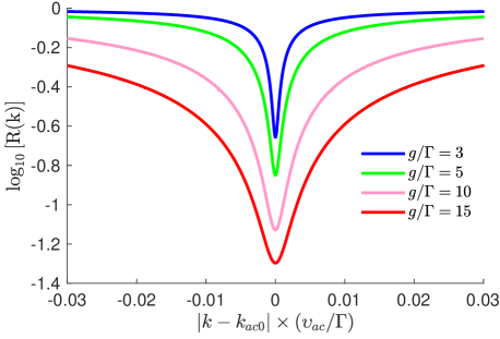
Figure 7: (Color online) Continuum optomechanical cooling versus wavenumber $k$ for different strong coupling strength $g/\Gamma=3,5,10,15$.

Appendix E Dynamical cooling generated by forward intermodal Brillouin scattering

In this section, we apply the modulation scheme of the optomechanical coupling intensity to the Brillouin cooling generated by the forward Brillouin anti-Stokes scattering in continuum optomechanical systems while optical dissipation exceeds mechanical dissipation Otterstrom . In order to achieve the Brillouin cooling, a critical requirement is the suppression of the Stokes scattering process. For the intra-modal Brillouin forward scattering, the Stokes process can not be suppressed since the Stokes and anti-Stokes waves interact through the same phonon mode Kharel , as shown in Fig. 8 (a). However, the dispersive symmetry between the Stokes and anti-Stokes processes can be broken for the inter-modal Brillouin forward scattering Chen ; Otterstrom when only the anti-Stokes process is engineered to satisfy the phase-matching condition, as shown in Fig. 8 (b). Here, we use the inter-modal forward anti-Stokes Brillouin scattering to study the phonon cooling.

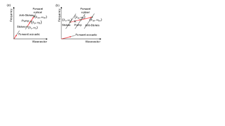
Figure 8: (Color online) Sketch of the dispersion diagram of forward Brillouin interaction for both intra-modal scattering (a) and inter-modal scattering (b).

Actually, similar to the backward Brillouin anti-Stokes scattering, there exists a Rabi oscillation of the phonon occupancy in the strong coupling regime for the forward Brillouin anti-Stokes scattering, which causes the reversible state swapping between phonons and anti-Stokes photons, i.e., swapping cooling and heating processes. If the size of the active-Brillouin waveguide is short enough which enables the Brillouin optomechanical interaction can be switched on and off by a pulsed pump, a dynamic cooling limit can be achieved by modulating the Brillouin optomechanical interaction to enhance the swapping cooling process while suppressing the heating process, which breaks the steady-state cooling limit.

Considering an un-depleted pump, the triply resonant Brillouin interaction can be reduced to an optomechanical interaction between anti-Stokes photons and acoustic phonons with a pump-enhanced coupling strength $g$. The dynamics of this reduced optomechanical interaction in the momentum space can be expressed as

$$\frac{d\tilde{a}}{dt} = \left(-\frac{\gamma}{2}+i\Delta_{1}\right)\tilde{a}-ig\tilde{b}+\sqrt{\gamma}\tilde{\xi}_{1},$$

$$\frac{d\tilde{b}}{dt} = \left(-\frac{\Gamma}{2}+i\Delta_{2}\right)\tilde{b}-ig\tilde{a}+\sqrt{\Gamma}\tilde{\xi}_{2},$$ (55)

where $\tilde{a}$ ($\tilde{b}$) denotes the annihilation operator of the anti-Stokes photons (acoustic phonons) corresponding to the $k$-th photon (phonon) mode. $\gamma$ ($\Gamma$) represents the optical (acoustic) dissipation. $\Delta_{1}=\upsilon_{o}k$ and $\Delta_{2}=\upsilon_{ac}k$ indicate the frequency shifts induced by the wavenumber $k$ for the anti-Stokes photons and acoustic phonons, respectively, where $\upsilon_{o}$ ($\upsilon_{ac}$) is the group velocity of the photons (phonons). $\tilde{\xi}_{1}$ and $\tilde{\xi}_{2}$ are the Langevin noises of the anti-Stokes field and the acoustic field, which obeys relationships

$$\langle\xi_{1}(t)\rangle = 0,$$

$$\langle\xi_{1}^{\dagger}(t_{1})\xi_{1}(t_{2})\rangle = 0,$$

$$\langle\xi_{1}(t_{1})\xi_{1}^{\dagger}(t_{1})\rangle = \delta(t_{1}-t_{2}),$$

$$\langle\xi_{2}(t)\rangle = 0,$$

$$\langle\xi_{2}^{\dagger}(t_{1})\xi_{2}(t_{2}) = n_{th}\delta(t_{1}-t_{2}),$$

$$\langle\xi_{2}(t_{1})\xi_{2}^{\dagger}(t_{2}) = (1+n_{th})\delta(t_{1}-t_{2}),$$ (56)

where $n_{th}$ correspond the thermal phonon occupation. Thus the differential equations for the second-order moments $\tilde{N}_{a}=\langle\tilde{a}^{\dagger}\tilde{a}\rangle$, $\tilde{N}_{b}=\langle\tilde{b}^{\dagger}\tilde{b}\rangle$, $\langle\tilde{a}^{\dagger}\tilde{b}\rangle$ can be given by

$$\frac{d\tilde{N}_{a}}{dt} = -\gamma\tilde{N}_{a}-ig\left[\langle\tilde{a}^{\dagger}\tilde{b}\rangle-\langle\tilde{a}^{\dagger}\tilde{b}\rangle^{*}\right],$$

$$\frac{d\tilde{N}_{b}}{dt} = -\Gamma\tilde{N}_{b}+ig\left[\langle\tilde{a}^{\dagger}\tilde{b}\rangle-\langle\tilde{a}^{\dagger}\tilde{b}\rangle^{*}\right]$$

$$+\frac{\Gamma n_{th}}{2\pi}\int_{-\infty}^{\infty}\frac{\gamma(g^{2}+\frac{\gamma\Gamma}{4})+\Gamma(\omega+\Delta_{1})^{2}}{\tilde{\Xi}_{1}}d\omega,$$

$$\frac{d\langle\tilde{a}^{\dagger}\tilde{b}\rangle}{dt} = -\left[i(\Delta_{1}-\Delta_{2})+\frac{\gamma+\Gamma}{2}\right]\langle\tilde{a}^{\dagger}\tilde{b}\rangle-ig\tilde{N}_{a}+ig\tilde{N}_{b}$$ (57)

$$+\frac{ig\Gamma n_{th}}{2\pi}\int_{-\infty}^{\infty}\frac{1}{\tilde{\Xi}_{2}}d\omega,$$

with

$$\tilde{\Xi}_{1} = \left[g^{2}+\frac{\gamma\Gamma}{4}-(\omega+\Delta_{1})(\omega+\Delta_{2})\right]^{2}$$

$$+\left[\frac{\gamma+\Gamma}{2}\omega+\frac{\gamma\Delta_{2}+\Gamma\Delta_{1}}{2}\right]^{2},$$

$$\tilde{\Xi}_{2} = g^{2}+\frac{\gamma\Gamma}{4}-(\omega+\Delta_{1})(\omega+\Delta_{2})$$ (58)

$$+i\left[\frac{\gamma+\Gamma}{2}\omega+\frac{\gamma\Delta_{2}+\Gamma\Delta_{1}}{2}\right],$$

where $\tilde{N}_{a}$ and $\tilde{N}_{b}$ correspond to the mean photon and phonon numbers. We consider the strong coupling regime ($g\gg\gamma,\Gamma$) and assume that the optical dissipation is far larger than the mechanical dissipation ($\gamma\gg\Gamma$) and the wavenumber induced frequency shifts are within the linewidth of the acoustic mode ($\Delta_{1,2}<\Gamma$). In addition, for the forward Brillouin scattering in a typical Brillouin-active waveguide, the velocity of the optical fields is greatly lager than the velocity of the acoustic field which leads to $\Delta_{1}\gg\Delta_{2}$ for $k\neq 0$. Thus the integral terms in Eq. (E) can be approximated to

$$\int_{-\infty}^{\infty}\frac{\gamma(g^{2}+\frac{\gamma\Gamma}{4})+\Gamma(\omega+\Delta_{1})^{2}}{\tilde{\Xi}_{1}}d\omega \approx 2\pi,$$

$$\int_{-\infty}^{\infty}\frac{1}{\tilde{\Xi}_{2}}d\omega \approx 0.$$ (59)

Substituting the above equations into Eq. (E), the analytical solution of the mean phonon number in the strong coupling regime can be expressed as

$$\tilde{N}_{b} \approx \tilde{C}_{1}e^{-\frac{\gamma+\Gamma}{2}t}+\tilde{C}_{2}e^{-\frac{\gamma+\Gamma}{2}t}\cos(\Omega t)$$ (60)

$$+\tilde{C}_{3}e^{-\frac{\gamma+\Gamma}{2}t}\sin(\Omega t)+\tilde{N}_{b}^{ss},$$

with

$$\tilde{C}_{1} \approx \frac{2g^{2}+\Delta_{1}^{2}-\frac{(\Gamma-\gamma)^{2}}{4}+\frac{(\gamma+\Gamma)^{2}}{4}}{\Omega^{2}}n_{th}$$

$$-\frac{4g^{2}+\Delta_{1}^{2}-\frac{(\Gamma-\gamma)^{2}}{4}+\frac{(\Gamma+\gamma)^{2}}{4}}{\Omega^{2}}\tilde{N}_{b}^{ss},$$

$$\tilde{C}_{2} \approx \frac{2g^{2}-\frac{(\Gamma+\gamma)^{2}}{4}}{\Omega^{2}}n_{th}+\frac{\frac{(\Gamma+\gamma)^{2}}{4}}{\Omega^{2}}\tilde{N}_{b}^{ss},$$

$$\tilde{C}_{3} \approx \frac{g\gamma-\frac{(\gamma+\Gamma)^{3}}{16g}}{\Omega^{2}}n_{th}+\frac{\frac{(\gamma+\Gamma)^{3}}{16g}}{\Omega^{2}}\tilde{N}_{b}^{ss},$$

$$\tilde{N}_{b}^{ss} \approx \frac{4g^{2}+\gamma(\gamma+\Gamma)}{4g^{2}+\gamma\Gamma}\cdot\frac{\Gamma}{\Gamma+\gamma}n_{th},$$

$$\Omega \approx \sqrt{4g^{2}+\Delta_{1}^{2}-\frac{(\Gamma-\gamma)^{2}}{4}},$$ (61)

where $\tilde{N}_{b}^{ss}$ denotes the steady-state cooling limit. We show the simulation results and the analytical solution of the time evolution for the phonon occupancy $\tilde{N}_{b}(t)$ in the strong coupling regime in Fig. 9 (a). It can be clearly seen that the strong optomechanical interaction enables the phonon occupancy to exhibit a Rabi oscillation with cycle $T=2\pi/\Omega$. The minimum value of the phonon occupancy can be achieved at the end of the first half Rabi oscillation cycle $t_{\rm{min}}=T/2$, which is much smaller than the steady-state cooling limit. Therefore, we switch off the pump at time $t_{\rm{min}}$ to halt the reversible Rabi oscillation and suppress the swapping heating process. After optical fields pass through the waveguide and are initialized to the vacuum state, we switch on the pump again to generate the swapping cooling process for absorbing phonons. We illustrate the modulation scheme and the corresponding time evolution of the phonon occupancy in Figs. 9 (b) and (c), respectively. By periodically initializing optical fields through a pulsed pump, the phonon occupancy can be continuously suppressed to an instantaneous-state cooling limit with a small-amplitude fluctuation, which breaks the steady-state cooling limit, as shown in Fig. 9 (c) where $\tau$ is the switch-off time. The instantaneous-state cooling limit, i.e., the lower cooling limit in Fig. 9 (c), can be evaluated at time $t_{\rm{min}}$ and approximately expressed as $\pi\Gamma n_{th}/(4g)$.

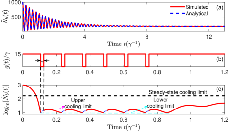
Figure 9: (Color online) (a) The time evolution of $\tilde{N}_{b}(t)$ in the strong coupling regime for $g/\gamma=15$. Modulation scheme of $g(t)$ with the switch-off time $\tau=0.1T$ (a) and the corresponding time evolution of the phonon occupancy (b). Other parameters are $\frac{\Gamma}{\gamma}=0.2$, $\frac{\Delta_{1}}{\gamma}=0.05$, $\frac{\Delta_{2}}{\gamma}=0.05\times 10^{-4}$, and $n_{th}=1000$.

In order to evaluate the upper cooling limit, we assume that switch-off time $\tau$ is small enough that the increase of the phonon occupancy during the switch-off time can be ignored. Then the analytical expression of $\tilde{N}_{b}(t)$ during time period $[T/2,T]$ can be given by

$$\tilde{N}_{b}(t) \approx \bar{C}_{1}e^{-\frac{\gamma+\Gamma}{2}(t-T/2)}+\bar{C}_{2}e^{-\frac{\gamma+\Gamma}{2}(t-T/2)}\cos(\Omega t)$$ (62)

$$+\bar{C}_{3}e^{-\frac{\gamma+\Gamma}{2}(t-T/2)}\sin(\Omega t)+\bar{N}_{b}^{ss},$$

where

$$\bar{C}_{1} \approx \frac{-16g^{2}+2\pi(\gamma+\Gamma)g}{4\Omega^{2}}\cdot\frac{\Gamma}{\Gamma+\gamma}n_{th},$$

$$\bar{C}_{2} \approx -\frac{2\pi(\gamma+\Gamma)g-(3\gamma^{2}+2\gamma\Gamma-\Gamma^{2})}{4\Omega^{2}}\cdot\frac{\Gamma}{\Gamma+\gamma}n_{th},$$

$$\bar{C}_{3} \approx -\frac{4g+\pi(\gamma-\Gamma)}{4\Omega^{2}}\Gamma n_{th},$$

$$\bar{N}_{b}^{ss} \approx \frac{4g^{2}+\gamma(\gamma+\Gamma)}{4g^{2}+\gamma\Gamma}\cdot\frac{\Gamma}{\Gamma+\gamma}n_{th},$$

$$\Omega \approx \sqrt{4g^{2}+\Delta_{1}^{2}-\frac{(\gamma-\Gamma)^{2}}{4}}.$$ (63)

The upper cooling limit in Fig. 9 (c) can be approximately calculated around time $t=3T/4$

$$\bar{N}_{b}^{\rm{upp}} \approx \bar{C}_{1}e^{-\frac{\gamma+\Gamma}{2}\frac{\pi}{2\Omega}}-\bar{C}_{3}e^{-\frac{\gamma+\Gamma}{2}\frac{\pi}{2\Omega}}+\bar{N}_{b}^{ss}$$ (64)

$$\approx \frac{(1+\pi)\Gamma}{4g}n_{th}.$$

Furthermore, this modulation scheme is switchable by turning on or off the modulation, as shown in Fig. 10.

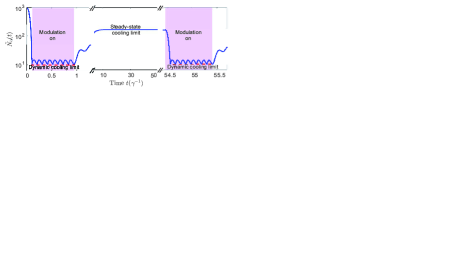
Figure 10: (Color online) The pulsed modulation is switchable.

References

• (1) M. D. LaHaye, O. Buu, B. Camarota, and K. C. Schwab, Approaching the Quantum Limit of a Nanomechanical Resonator, Science 304, 74 (2004).
• (2) J. D. Teufel, T. Donner, M. A. Castellanos-Beltran, J. W. Harlow, and K. W. Lehnert, Nanomechanical motion measured with an imprecision below that at the standard quantum limit, Nat. Natotech. 4, 820 (2009).
• (3) T. P. Purdy, R. W. Peterson, and C. A. Regal, Observation of radiation pressure shot noise on a macroscopic object, Science 339, 801 (2013).
• (4) T. A. Palomaki, J. D. Teufel, R. W. Simmonds, and K. W. Lehnert, Entangling mechanical motion with microwave fields, Science 342, 710 (2013).
• (5) R. Riedinger, A. Wallucks, I. Marinković, C. Löschnauer, M. Aspelmeyer, S. Hong and S. Gröblacher, Remote quantum entanglement between two micromechanical oscillators, Nature (London) 556, 473 (2018).
• (6) C. F. Ockeloen-Korppi, E. Damskägg, J. M. Pirkkalainen, M. Asjad, A. A. Clerk, F. Massel, M. J. Woolley, and M. A. Sillanpää, Stabilized entanglement of massive mechanical oscillators, Nature (London) 556, 478 (2018).
• (7) W. Marshall, C. Simon, R. Penrose, and D. Bouwmeester, Towards Quantum Superpositions of a Mirror, Phys. Rev. Lett. 91, 130401 (2003).
• (8) I. Pikovski, M. R. Vanner, M. Aspelmeyer, M. S. Kim, and C̆. Brukner, Probing Planck-scale physics with quantum optics, Nat. Phys. 8, 393 (2012).
• (9) M. Arndt and K. Hornberger, Testing the limits of quantum mechanical superpositions, Nat. Phys. 10, 271 (2014).
• (10) J. D. Teufel, T. Donner, D. Li, J. H. Harlow, M. S. Allman, K. Cicak, A. J. Sirois, J. D. Whittaker, K. W. Lehnert, and R. W. Simmonds, Sideband cooling of micromechanical motion to the quantum ground state, Nature (London) 475, 395 (2011).
• (11) J. Chan, T. P. Mayer Alegre, A. H. Safavi-Naeini, J. T. Hill, A. Krause, S. Gröblacher, M. Aspelmeyer, and O. Painter, Laser cooling of a nanomechanical oscillator into its quantum ground state, Nature (London) 478, 89 (2011).
• (12) L. Qiu, I. Shomroni, P. Seidler, and T. J. Kippenberg, Laser Cooling of a Nanomechannical Oscillator to Its Zero-Point Energy, Phys. Rev. Lett. 124, 173601 (2020).
• (13) M. Aspelmeyer, T. J. Kippenberg, and F. Marquardt, Cavity optomechanics, Rev. Mod. Phys. 86, 1391 (2014).
• (14) R. W. Boyd, Nonlinear Optics (Academic Press, New York, 2008).
• (15) G. P. Agrawal, Nonlinear Fiber Optics (Academic Press, San Diego, 2007).
• (16) M. Tomes and T. Carmon, Photonic Micro-Electromechanical Systems Vibrating at X-band (11-GHz) Rates, Phys. Rev. Lett. 102, 113601 (2009).
• (17) M. Tomes, F. Marquardt, G. Bahl, and T. Carmon, Quantum-mechanical theory of optomechanical Brillouin cooling, Phys.Rev. A 84, 063806 (2011).
• (18) G. Bahl, M. Tomes, F. Marquardt, and T. Carmon, Observation of spontaneous Brillouin cooling, Nat. Phys. 8, 203 (2012).
• (19) C. H. Dong, Z. Shen, C. Ling Zou, Y. Lei Zhang, W. Fu, and G. C Guo, Brillouin-scattering-induced transparency and non-reciprocal light storage, Nat. Commun. 6, 6193 (2015).
• (20) Z. Shen, Y. L. Zhang, Y. Chen, C. L Zou, Y. F. Xiao, X. B. Zou, F. W. Sun, G. C. Guo, and C. H. Dong, Experimental realization of optomechanically induced non-reciprocity, Nat. Photonics 10, 657 (2016).
• (21) G. Enzian, M. Szczykulska, J. Silver, L. Del Bino, S. Zhang, I. A. Walmsley, P. Del’Haye, and M. R. Vanner, Observation of Brillouin optomechanical strong coupling with an 11 GHz mechanical mode, Optica 6, 7 (2019).
• (22) Y. C. Chen, S. Kim, and G. Bahl, Brillouin cooling in a linear waveguide, New J. Phys. 18, 115004 (2016).
• (23) N. T. Otterstrom, R. O. Behunin, E. A. Kittlaus, and P. T. Rakich, Optomechanical Cooling in a Continuous system, Phys. Rev. X 8, 041034 (2018).
• (24) B. J. Eggleton, C. G. Poulton, P. T. Rakich, M. J. Steel, and G. Bahl, Brillouin integrated photonics, Nat. Photonics 13, 664 (2019).
• (25) M. Merklein, B. Stiller, K. Vu, S. J. Madden, and B. J. Eggleton, A chip-integrated coherent photonic-phononic memory, Nat. Commun. 8, 574 (2017).
• (26) R. Van Laer, R. Baets, and D. Van Thourhout, Unifying Brillouin scattering and cavity optomechanics, Phys. Rev. A 93, 053828 (2016).
• (27) K. P. Huy, J. C. Beugnot, J. C. Tchahame, and T. Sylvestre, Strong coupling between phonons and optical beating in backward Brillouin scattering, Phys. Rev. A 94, 043847 (2016).
• (28) E. Verhagen, S. Deléglise, S. Weis, A. Schliesser, and T. J. Kippenberg, Quantum-coherent coupling of a mechanical oscillator to an optical cavity mode, Nature (London) 482, 63 (2012).
• (29) A. H. Safavi-Naeini, D. V. Thourhout, R. Baets, and R. V. Laer, Controlling phonons and photons at the wavelength scale: integrated photonics meets integrated phononics, Optica 6, 213 (2019).
• (30) W. K. Hensinger, D. W. Utami, H. S. Goan, K. Schwab, C. Monroe, and G. J. Milburn, Ion trap transducers for quantum electromechanical oscillators, Phys. Rev. A 72, 041405(R) (2005).
• (31) L. Tian, M. S. Allman, and R. W. Simmonds, Parametric cooling between macroscopic quantum resonators, New J. Phys. 10, 115001 (2008).
• (32) L. Tian and H. L. Wang, Optical wavelength conversion of quantum states with optomechanics, Phy. Rev. A 82, 053806 (2010).
• (33) X. T. Wang, S. Vinjanampathy, F. W. Strauch, and K. Jacobs, Ultraefficient Cooling of Resonators: Beating Sideband Cooling with Quantum Control, Phys. Rev. Lett. 107, 177204 (2011)
• (34) Y. C. Liu, Y. F. Xiao, X. S. Luan and C. W. Wong, Dynamical Dissipative Cooling of a Mechanical Resonator in Strong Coupling Optomechanics, Phys. Rev. Lett. 110, 153606 (2013).
• (35) P. Kharel, R. O. Behunin, W. H. Renninger, and P. T. Rakich, Noise and dynamics in forward Brillouin interactions, Phys. Rev. A 93, 063806 (2016).
• (36) J. E. Sipe and M. J. Steel, A Hamiltonian treatment of Stimulated Brillouin scattering in nanoscale integrated waveguides, New. J. Phys. 18, 045004 (2016).
• (37) H. Zoubi and K. Hammerer, Optomechanical multimode Hamiltonian for nanophotonic waveguides, Phys. Rev. A 94, 053827 (2016).
• (38) R. W. Boyd, K. Rzazewski, and P. Narum, Noise initiation of stimulated Brillouin scattering, Phys. Rev. A 42, 5514 (1990).
• (39) P. Rakich and F. Marquardt, Quantum theory of continuum optomechanics, New. J. Phys. 20, 045005 (2018).
• (40) I. Wilson-Rae, N. Nooshi, W. Zwerger, and T. J. Kippenberg, Theory of Ground State Cooling of a Mechanical Oscillator Using Dynamical Backaction, Phys. Rev. Lett. 99, 093901 (2007).
• (41) F. Marquardt, J. P. Chen, A. A. Clerk, and S. M. Girvin, Quantum Theory of Cavity-Assisted Sideband Cooling of Mechanical Motion, Phys. Rev. Lett. 99, 093902 (2007).
• (42) C. Genes, D. Vitali, P. Tombesi, S. Gigan, and M. Aspelmeyer, Ground-state cooling of a micromechanical oscillator: Comparing cold damping and cavity-assisted cooling schemes, Phys. Rev. A 77, 033804 (2008).
• (43) S. Machnes, J. Cerrillo, M. Aspelmeyer, W. Wieczorek, M. B. Plenio, and A. Retzker, Pulsed Laser Cooling for Cavity Optomechanical Resonators, Phys. Rev. Lett. 108, 153601 (2012).