Contrastive Learning for Joint Normal Estimation
and Point Cloud Filtering

Abstract

Point cloud filtering and normal estimation are two fundamental research problems in the 3D field. Existing methods usually perform normal estimation and filtering separately and often show sensitivity to noise and/or inability to preserve sharp geometric features such as corners and edges. In this paper, we propose a novel deep learning method to jointly estimate normals and filter point clouds. We first introduce a 3D patch based contrastive learning framework, with noise corruption as an augmentation, to train a feature encoder capable of generating faithful representations of point cloud patches while remaining robust to noise. These representations are consumed by a simple regression network and supervised by a novel joint loss, simultaneously estimating point normals and displacements that are used to filter the patch centers. Experimental results show that our method well supports the two tasks simultaneously and preserves sharp features and fine details. It generally outperforms state-of-the-art techniques on both tasks. Our source code is available at https://github.com/ddsediri/CLJNEPCF.

Point cloud filtering, normal estimation, contrastive learning, machine learning.

1 Introduction

Point clouds have numerous applications as they provide a natural representation of 3D geometric information. They have seen applications in fields such as autonomous driving, robotics, 3D printing and urban planning [Luo-Pillar-Motion, Bekiroglu-PCD-Robotics, Kim-3D-Printing, Urech-Urban-Planning]. Captured using 3D sensors, point clouds consist of unordered points which lack connectivity information between individual points. The captured point cloud information may be corrupted with noise. Therefore, one fundamental research problem is point cloud filtering, also known as denoising. Another fundamental task is normal estimation at individual points. Together, they facilitate other tasks such as 3D rendering and surface reconstruction.

Conventional normal estimation methods, such as Principal Component Analysis (PCA) and its variants [Hoppe-PCA, Mitra-Estimating-Surface-Normals, Pauly-Point-Sampled, Yoon-Surface-Normal-Ensembles] and Voronoi diagram based approaches [Amenta-Surface-Voronoi, Alliez-Voronoi-Variational, Dey-Voronoi-based-Normal-Estimation], perform poorly when estimating the normals at sharp features such as corners or edges and show high sensitivity to noise. To address these issues, a number of learning based methods have been recently proposed such as Deep Feature Preserving (DFP) [Lu-Deep-Feature-Preserving] and Nesti-Net [Ben-Shabat-Nesti-Net]. However, they have large network sizes and therefore are typically slow. Methods such as AdaFit [Zhu-AdaFit] and Deep Iterative (DI) [Lenssen-Deep-Iterative] offer more lightweight solutions that perform admirably, but still show less robust results at higher noise levels.

Point cloud filtering can be classified into two main types: normal based methods [RIMLS-Oztireli, Sun-L0, Avron-L1, Lu-Deep-Feature-Preserving] and position based methods [Lipman-LOP, Huang-WLOP, Rakotosaona-PCN, Zhang-Pointfilter]. The former utilizes normal information at a given point in order to apply a position update algorithm [Lu-Deep-Feature-Preserving], while the latter does not require normal information and relies solely on position information. Among position based methods, a common issue is the inability to preserve sharp features during the filtering process while normal based methods rely heavily on normal accuracy. Learning based approaches seek to resolve this. In particular, Pointfilter [Zhang-Pointfilter], performs effectively at preserving sharp feature information on CAD-like shapes yet fails to generalize to large scenes. Methods such as PointCleanNet [Rakotosaona-PCN] and TotalDenoising [Hermosilla-Total-Denoising] also perform sub-optimally, tending to smear sharp features.

In this paper, we propose a novel method capable of simultaneously inferring point normals and displacements while maintaining robustness to noise. Our method comprises of a feature encoder capable of generating latent representations of patches based on patch similarity and a regressor capable of inferring point normals and displacements simultaneously. We introduce a 3D patch based contrastive learning framework to train the feature encoder which employs noise corruption as an augmentation technique, allowing the encoder to identify the sharp geometric features of the underlying clean patch despite different levels of noise corruptions. The regressor consumes the latent representation of a patch and outputs the point normal and the displacement required to filter the central point of that patch. To train the regressor, we introduce a novel loss function that jointly penalizes inferred point position error and normal estimation error by exploiting the relationship between a point’s position and normal. We intuitively assume that a filtered point’s normal should correspond to a ground truth point’s normal if this ground truth point first corresponds to that filtered point in position, thus leading to the relationship between filtering and normal estimation.

The main contributions of this paper are as follows.

• We develop a novel framework capable of inferring both points’ displacements and normals simultaneously by introducing a loss function capable of constraining both filtering and normal estimation tasks. This joint loss penalizes both position regression error and normal estimation prediction error and allows the network to learn both filtered displacements and point normals.

• We introduce 3D patch based contrastive learning to generate effective patch-wise representations.

We conduct extensive experiments and demonstrate that our method, in general, outperforms state-of-the-art normal estimation and filtering techniques.

2 Related work

Normal estimation. In its earliest incarnation, normal estimation was based on Principal Component Analysis (PCA) [Hoppe-PCA]. Several variants of this initial PCA method have also been proposed [Mitra-Estimating-Surface-Normals, Pauly-Point-Sampled, Yoon-Surface-Normal-Ensembles]. Thereafter, approaches based on Voronoi cells were used to reconstruct surfaces while preserving sharp features and estimating normals [Amenta-Surface-Voronoi, Alliez-Voronoi-Variational, Dey-Voronoi-based-Normal-Estimation]. Recently, Lu et al. [Lu-Low-Rank] proposed a normal estimation method based on a Low Rank Matrix Approximation (LRMA) algorithm. Additionally, methods such as [Li-Robust-Sharp-Features, Zhang-Guided-Least-Squares, Zhang-Low-Rank, Zhang-Pair-Consistency-Voting] utilized point statistics and clustering to determine point normals.

Normal estimation (learning-based). One of the first learning models for normal estimation, HoughCNN, employs a voting mechanism for estimating normals. They utilize a local patch representation in Hough space that can be consumed by a CNN [Boulch-HoughCNN]. However, with the advent of PointNet [Qi-PointNet] and PointNet++ [Qi-PointNet++], newer methods have been proposed that directly consume point sets. PCPNet is one such example, which consumes point cloud patches at multiple scales [Guerrero-PCPNet]. Similarly, Nesti-Net consumes patches at multiple scales but also employs multiple sub-networks, Mixture-of-Experts, that specialize in estimating normals at these scales [Ben-Shabat-Nesti-Net]. Wang and Prisacariu introduced NINormal, a self-attention based normal estimation scheme [Wang-NINormal] while Lu et al. proposed Deep Feature Preserving (DFP), a two step mechanism that classifies points into feature and non-feature points and, subsequently, estimates their normals based on this classification [Lu-Deep-Feature-Preserving]. Finally, several deep learning methods based on weighted least squares plane fitting have been proposed [Lenssen-Deep-Iterative, Ben-Shabat-DeepFit, Zhu-AdaFit]. While these methods focus on accurately determining unoriented normals, the work of Wang et al. [Wang-Deep-Global-NO] focuses on estimating point normals and their orientations.

Point cloud filtering. Traditional filtering applications center around Moving Least Squares (MLS) approaches [MLS-Levin, Kolluri-MLS]. Alexa et al. [Alexa--MLS-PSS] built on MLS techniques to minimize the approximation error of denoised point set surfaces. These methods perform poorly on point sets with sharp features, an issue that Adamson and Alexa [IMLS-Adamson] and Guennebaud and Gross [APSS-Guennebaud] aimed to tackle. Lipman et al. developed the Locally Optimal Projection (LOP) operator which does not depend on a local data parametrization such as a local normal or tangent plane [Lipman-LOP]. This projection operator was further enhanced by Huang et al. and Preiner et al., who proposed a Weighted LOP (WLOP) [Huang-WLOP] and Continuous LOP (CLOP) [Preiner-CLOP], respectively. The main drawback to these MLS and LOP based techniques is their inability to preserve sharp features. Oztireli, Guennebaud and Gross [RIMLS-Oztireli] proposed Robust Implicit Moving Least Squares [RIMLS-Oztireli] which improves the filtering ability to preserve sharp features but relies heavily on the accuracy of normal information. Lu et al. proposed a point cloud filtering scheme based on normals estimated by their LRMA algorithm [Lu-Low-Rank]. Remil et al. reformulated point cloud filtering as a global, sparse optimization problem which is solved using Augmented Lagrangian Multipliers [Remil-Data-Driven-Sparse-Priors].

Point cloud filtering (learning-based). PointProNets used a CNN which consumes noisy height-maps and returns filtered ones [Roveri-PointProNets]. EC-Net employed a supervised scheme for edge aware filtering and upsampling [Yu-EC-Net]. PCN uses a $L_{1}$ norm loss based network to remove outliers and $L_{2}$ norm loss based network to filter points [Rakotosaona-PCN]. Pointfilter takes into account local structure by considering points and their ground-truth normals, during training time, to infer filtered positions [Zhang-Pointfilter]. DFP [Lu-Deep-Feature-Preserving] employs the position update mechanism of [Lu-Low-Rank] to filter points based on the estimated normals. ScoreDenoise (SD) models a noisy point cloud’s underlying surface with a 3D distribution supported by 2D manifolds and estimates the score for the gradient of the noise convolved distribution [Luo-Score-Based-Denoising]. TotalDenoising (TD) offers an unsupervised learning alternative to the aforementioned supervised schemes [Hermosilla-Total-Denoising].

Contrastive learning. Recently, we have seen the increased use of contrastive learning in generating faithful representations based on similarity between inputs. Self-supervised learning that maximizes agreement between similar inputs was first proposed by Becker and Hinton [Becker-Contrastive]. Thereafter, contrastive learning was further exploited to learn lower dimensional representations of high dimensional image data by the work of Hadsell, Chopra and LeCun [Hadsell-Contrastive]. Chen et al. utilized more recent neural network architectures and data augmentation methods in their SimCLR method [Chen-SimCLR]. Although initially designed for 2D image processing tasks, contrastive learning is now seeing applications in 3D representation learning [jiang2021unsupervised, Lal-CoCoNets, Du-Self-Supervised-Point-Cloud, Afham-CrossPoint] and for specific point cloud processing tasks such as shape completion, segmentation and scene understanding [Alliegro-Shape-Completion, Li-HybridCR, Hou-3D-Scene]. However, it has never before been explored in terms of the problems of normal estimation and point cloud filtering, which we focus on in this work.

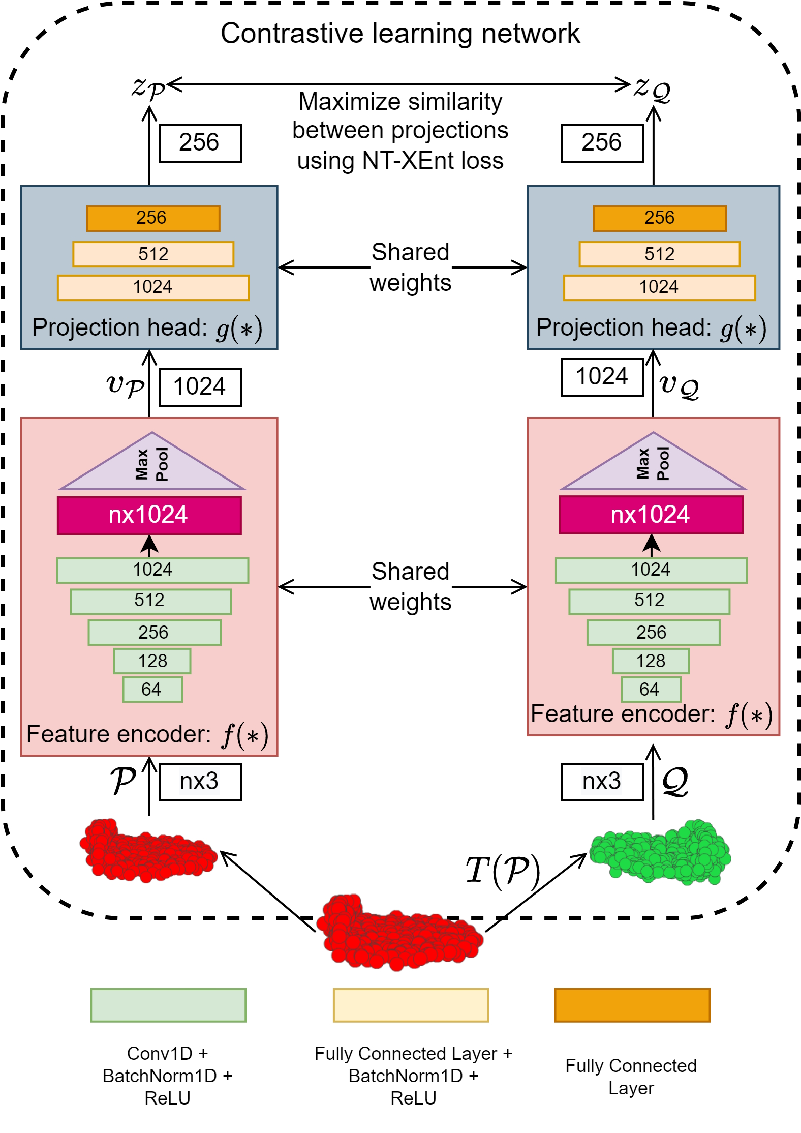
Figure 1: 3D patch based contrastive learning.

3 Background and Motivation

In this section, we look at the motivation for our contrastive learning based joint normal estimation and filtering method.

3.1 Patch-based contrastive learning

As mentioned earlier, contrastive learning has emerged as an effective method of generating latent representations of inputs such as images or point clouds based on similarity between augmented pairs of inputs which are seen by the network during training [Chen-SimCLR]. The work of Xie et al. [Xie-PointContrast] extended this method to 3D point clouds. Crucially, their work focuses on generating representations of entire point clouds, i.e., they use a global approach. However, as Guerrero et al. [Guerrero-PCPNet] point out, normal estimation at a given point relies on the local structure of the point neighborhood rather than the global structure of the entire point cloud. This is also true for the problem of point cloud filtering [Rakotosaona-PCN] as effective filtering mechanisms must preserve sharp feature information locally. This motivates our approach of developing a patch-based contrastive learning mechanism where noise corruption of input patches is used as an augmentation to develop different views of the same underlying clean patch. Thereafter, we employ the Normalized Temperature-scaled Cross Entropy (NT-XEnt) loss function detailed in Sec. LABEL:sec:contrastive-learning which promotes similarity of generated latent representations for a given positive pair of augmented patches. Inspired by the work of [Chen-SimCLR], we do not explicitly sample negative pairs as the remaining augmented pairs within a batch can be used for this purpose. Furthermore, the goal of this contrastive process is to bring representations of patches of the same underlying clean structure closer together, which is unlike a triplet based learning process which simultaneously brings representations closer for similar patches while pushing away representations of dissimilar patches.

3.2 Joint normal estimation and filtering

Normal estimation and point cloud filtering are two interconnected tasks. Accurately predicted normals are central to reliable point cloud filtering and surface reconstruction as mentioned by [Lu-Deep-Feature-Preserving, RIMLS-Oztireli]. In a similar manner, predicting normals on less noisy patches provide more accurate results, as opposed to noisier patches where outliers affect the final prediction [Guerrero-PCPNet, Lenssen-Deep-Iterative]. This motivates our joint normal estimation and filtering approach where our regression network estimates patch normals along with point displacements to filter central patch points. Thereafter, the estimated normals are used to further refine the final filtered position. This approach helps exploit the interlinked relationship between normal estimation and point cloud filtering and motivates our joint approach.

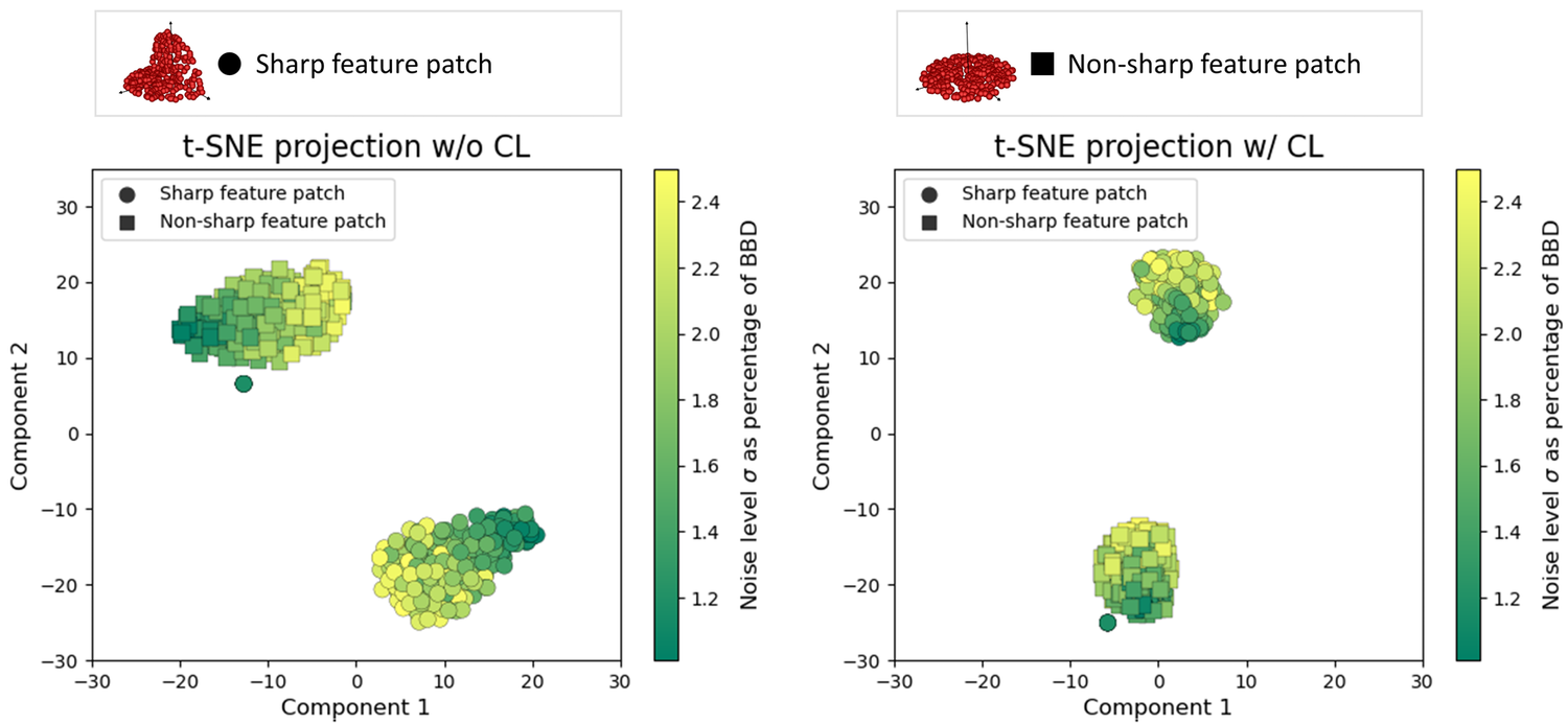
Figure 2: The impact of using a feature encoder pretrained using contrastive learning compared to a feature encoder trained from scratch. We consider t-SNE projections of latent representations of a sharp feature patch and a non-sharp feature patch at different Gaussian noise levels $\sigma$, w.r.t. the bounding box diagonal (BBD) of the clean point cloud. Respective clean patches are illustrated at the top.

3.3 Link between contrastive learning and regression tasks

Feature encoders trained using contrastive learning are adept at generating similar representations of similar inputs and dissimilar representations of dissimilar inputs. Guided by the intuition that two noisy variants of the same underlying clean patch should generate similar latent representations, we develop a contrastive learning framework with noise corruption as an augmentation to train a feature encoder $f(\ast)$ (see Fig. 1). This encoder is later used as part of a regression network (Fig. 3) to infer point normals and filtered displacements simultaneously. During training of the regression network, the pretrained feature encoder’s weights are kept frozen and only the regressor $h(\ast)$ is trained. The pretrained feature encoder is robust to noise and generates representations that can be consumed more effectively by the regression network during training. Fig. 2 illustrates t-SNE projections of 250 noisy variants of a given sharp feature patch and 250 noisy variants of a non-sharp feature patch obtained from the Cube shape in our dataset. The corresponding clean patches are illustrated at the top of Fig. 2. Each noisy variant contains Gaussian noise of standard deviation $\sigma$, ranging from $1.0\%$ to $2.5\%$ of the clean point cloud’s bounding box diagonal. We observe that a feature encoder trained without contrastive learning generates latent representations that are less similar for differing noisy patch variants sharing a common underlying clean structure, for both the sharp feature and non-sharp feature patch. This is evident from Fig. 2 as low noise patch variants (dark green markers) have projections that are far apart from their respective higher noise counterparts (light green/yellow markers).

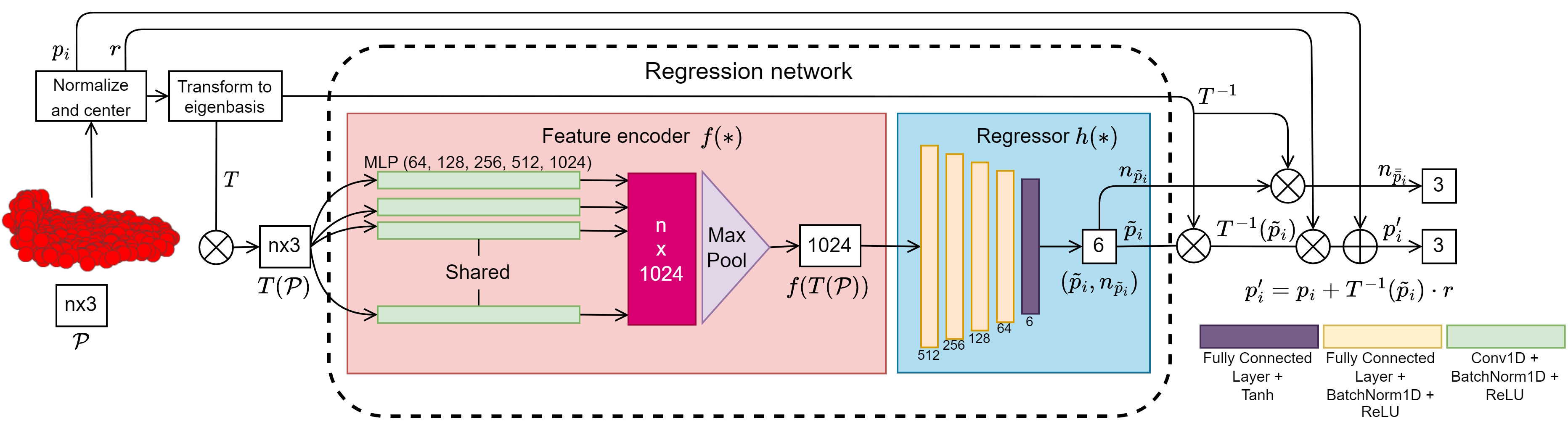
Figure 3: Overview of the Regression network for outputting filtered points and normals. Feature encoder is taken from contrastive learning.

The feature encoder pretrained using contrastive learning, with only noise corruption as an augmentation, generates latent representations whose t-SNE projections are clustered more closely, indicating that representations are more similar even as noise increases. This is due to the contrastive pretraining that exploits noise corruption as an augmentation and ensures robustness to noise. As such, latent representations generated by the feature encoder are easier for the regression network to distinguish, even for high noise patches, as these representations are similar to that of the underlying clean counterparts. Thereby, the contrastive learning based pretraining facilitates our joint normal estimation and point cloud filtering method.

4 Proposed Methodology

4.1 Overview

We first introduce 3D patch-based contrastive learning to train a feature encoder capable of producing representations of point cloud patches (Fig. 1). This feature encoder consists of a PointNet-like architecture, with 5 Conv1D layers and a global max pool layer that generates a 1024 dimensional representation of input point cloud patches. These representations are projected to a 256 dimensional vector by a projection head consisting of 3 fully connected layers. Once the feature encoder has been trained, we use it to generate latent representations of input patches for regression tasks. Next, we train a regression network (Fig. 3) to predict patch normals and displacements simultaneously (i.e., normal and displacement of the central point of a patch). The regressor consists of the pretrained feature encoder and a MLP of 5 fully connected layers that output the desired normals and displacements. During the testing phase, these displacements are added to the initial point cloud, which produces a filtered point cloud that is refined and becomes the input for the next iteration of inference.

4.2 Contrastive pair construction

A clean point cloud consisting of $n$ points is described by $\mathbf{P}_{s}=\{p_{i}\ |\ p_{i}\in\mathbb{R}^{3},\ i\ =1,...,n\}$ where $s=1,\ldots,M$ enumerates all training shapes. A noisy point cloud $\hat{\mathbf{P}}_{s}$ can, thereafter, be characterized by the addition of noise onto the clean point cloud

$$\hat{\mathbf{P}}_{s}(\sigma) =\mathbf{P}_{s}+\mathbf{N}(0,\sigma^{2}),$$ (1)

where $\mathbf{N}(0,\sigma^{2})$ corresponds to additive Gaussian noise with a mean of $0$ and standard deviation of $\sigma$. For our training set, $\sigma$ takes on values of 0.25%, 0.5%, 1.0%, 1.5% and 2.5% of the bounding box diagonal length of $\mathbf{P}_{s}$. For a given shape, the set of 6 variant point clouds (1 clean and 5 noisy), is given by