Partial Differential Equations of Mixed Type
— Analysis and Applications

Partial differential equations (PDEs) are at the heart of many mathematical and scientific advances. While great progress has been made on the theory of PDEs of standard types during the last eight decades, the analysis of nonlinear PDEs of mixed type is still in its infancy. The aim of this expository paper is to show, through several longstanding fundamental problems in fluid mechanics, differential geometry, and other areas, that many nonlinear PDEs arising in these areas are no longer of standard types, but lie at the boundaries of the classification of PDEs or, indeed, go beyond the classification to be of mixed type. Some interrelated connections, historical perspectives, recent developments, and current trends in the analysis of nonlinear PDEs of mixed type are also presented.

1. Linear Partial Differential Equations of Mixed Type

Three of the basic types of PDEs are the elliptic, hyperbolic, and parabolic types, following the classification introduced by Jacques Salomon Hadamard in 1923 (see Fig. 2).

The prototype of second-order elliptic equations is the Laplace equation:

$$\Delta_{\bf x}u:=\sum_{j=1}^{n}\partial_{x_{j}x_{j}}u=0\qquad\quad\mbox{for ${\bf x}=(x_{1},\dots,x_{n})\in\mathbb{R}^{n}$},$$ (1.1)

often describing physical equilibrium states, whose solutions are also called harmonic functions or potential functions, where $\partial_{x_{j}x_{j}}$ is the second-order partial derivative in the $x_{j}$-variable, $j=1,\dots,n$. The simplest representative of hyperbolic equations is the wave equation:

$$\partial_{tt}u-\Delta_{\bf x}u=0\qquad\quad\mbox{for $(t,{\bf x})\in\mathbb{R}^{n+1}$},$$ (1.2)

which governs the propagation of linear waves (such as acoustic waves and electromagnetic waves), while the prototype of second-order parabolic equations is the heat equation:

$$\partial_{t}u-\Delta_{\bf x}u=0\qquad\quad\mbox{for $(t,{\bf x})\in\mathbb{R}^{n+1}$},$$ (1.3)

which often describes the dynamics of temperature and diffusion/stochastic processes.

Figure 1.         Jacques Salomon Hadamard (8 December 1865 – 17 October 1963) first introduced the classification of PDEs in [16]

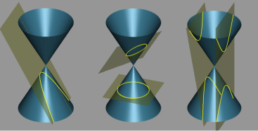
Figure 2.    Types of conic sections: Parabola, ellipse, and hyperbola

At first glance, the forms of the Laplace/heat equations and the wave equation look quite similar. In particular, any steady solution of the wave/heat equations is a solution of the Laplace equation, while a solution of the Laplace equation often determines an asymptotic state of the time-dependent solutions of the wave/heat equations. However, the properties of solutions of the Laplace/heat equations and the wave equation are significantly different. One difference is the infinite versus finite speed of propagation of the solution, while another is the gain versus loss of regularity of the solution; see [14, 16] and the references cited therein. Since the solutions of elliptic/parabolic PDEs share many common features, we will focus mainly on PDEs of mixed elliptic-hyperbolic type from now on.

The distinction between the elliptic and hyperbolic types can be seen more clearly from the classification of two-dimensional ($2$-D) constant-coefficient second-order PDEs:

$$a_{11}\partial_{x_{1}x_{1}}u+2a_{12}\partial_{x_{1}x_{2}}u+a_{22}\partial_{x_{2}x_{2}}u=f({\bf x})\qquad\quad\,\,\mbox{for $\,{\bf x}=(x_{1},x_{2})\in\mathbb{R}^{2}$}.$$ (1.4)

Let $\lambda_{1}\leq\lambda_{2}$ be the two constant eigenvalues of the $2\times 2$ symmetric coefficient matrix $(a_{ij})_{2\times 2}$. Eq. (1.4) is classified to be elliptic if

$$\det(a_{ij})>0\iff\lambda_{1}\lambda_{2}>0\iff a_{12}^{2}-a_{11}a_{22}<0,$$ (1.5)

while Eq. (1.4) is classified to be hyperbolic if

$$\det(a_{ij})<0\iff\lambda_{1}\lambda_{2}<0\iff a_{12}^{2}-a_{11}a_{22}>0.$$ (1.6)

Notice that the left-hand side of Eq. (1.4) is analogous to the quadratic (homogeneous) form:

$$a_{11}\xi_{1}^{2}+a_{12}\xi_{1}\xi_{2}+a_{22}\xi_{2}^{2}$$

for conic sections. Thus, the classification of Eq. (1.4) is consistent with the classification of conic sections and quadratic forms in algebraic geometry, based on the sign of the discriminant: $a_{12}^{2}-a_{11}a_{22}$. The corresponding quadratic curves are ellipses (incl. circles), hyperbolas, and parabolas (see Fig. 2).

This classification can also be seen through taking the Fourier transform on both sides of Eq. (1.4):

$$(a_{11}\xi_{1}^{2}+2a_{12}\xi_{1}\xi_{2}+a_{22}\xi_{2}^{2})\,\hat{u}({\bm{\xi}})=-\hat{f}({\bm{\xi}})\qquad\quad\,\,\mbox{for $\,{\bm{\xi}}=(\xi_{1},\xi_{2})\in\mathbb{R}^{2}$},$$ (1.7)

where $\hat{w}({\bm{\xi}})=\frac{1}{2\pi}\int_{-\infty}^{\infty}w({\bf x})e^{-i{\bf x}\cdot{\bm{\xi}}}\,{\rm d}{\bf x}$ is the Fourier transform of a function $w({\bf x})$, such as $u({\bf x})$ and $f({\bf x})$ for (1.7). When Eq. (1.4) is elliptic, the Fourier transform $\hat{u}({\bm{\xi}})$ of the solution $u({\bf x})$ gains two orders of decay for the high Fourier frequencies (i.e., $|{\bm{\xi}}|\gg 1$) so that the solution gains the regularity of two orders from $f({\bf x})$. When Eq. (1.4) is hyperbolic, $\hat{u}({\bm{\xi}})$ fails to gain two orders of decay for the high Fourier frequencies along the two characteristic directions in which $a_{11}\xi_{1}^{2}+2a_{12}\xi_{1}\xi_{2}+a_{22}\xi_{2}^{2}=0$, even though it still gains two orders of decay for the high Fourier frequencies away from these two directions.

For the classification above, a general homogeneous constant-coefficient second-order PDE (i.e., $f({\bf x})=0$) with (1.5) or (1.6) can be transformed into the Laplace equation (1.1) with $n=2$, or the wave equation (1.2) with $n=1$, via the corresponding coordinate transformations, respectively. This exposes the beauty of the classification theory introduced first in Hadamard [16].

On the other hand, for general variable-coefficient second-order PDEs:

$$a_{11}(\mathbf{x})\partial_{x_{1}x_{1}}u+2a_{12}(\mathbf{x})\partial_{x_{1}x_{2}}u+a_{22}(\mathbf{x})\partial_{x_{2}x_{2}}u=f({\bf x}),$$ (1.8)

the situation is different. The classification depends upon the signature of the eigenvalues $\lambda_{j}(\mathbf{x}),j=1,2$, of the coefficient matrix $(a_{ij}(\mathbf{x}))$. In general, $\lambda_{1}(\mathbf{x})\lambda_{2}(\mathbf{x})$ may change its sign as a function of ${\bf x}$, which leads to the mixed elliptic-hyperbolic type of (1.8): Eq. (1.8) is elliptic when $\lambda_{1}(\mathbf{x})\lambda_{2}(\mathbf{x})>0$ and hyperbolic when $\lambda_{1}(\mathbf{x})\lambda_{2}(\mathbf{x})<0$ with transition boundary/region where $\lambda_{1}(\mathbf{x})\lambda_{2}(\mathbf{x})=0$.

Three of the classical prototypes for linear PDEs of mixed elliptic-hyperbolic type are:

(i) The Lavrentyev-Bitsadze equation: $\qquad\partial_{x_{1}x_{1}}u+{\rm sign}(x_{1})\partial_{x_{2}x_{2}}u=0$.

This equation exhibits a jump transition at $x_{1}=0$. It becomes the Laplace equation (1.1) in the half-plane $x_{1}>0$ and the wave equation (1.2) in the half-plane $x_{1}<0$, and changes its type from elliptic to hyperbolic via the jump-discontinuous coefficient ${\rm sign}(x_{1})$.

(ii) The Tricomi equation: $\qquad\partial_{x_{1}x_{1}}u+x_{1}\partial_{x_{2}x_{2}}u=0$.

This equation is of hyperbolic degeneracy at $x_{1}=0$. It is elliptic in the half-plane $x_{1}>0$ and hyperbolic in the half-plane $x_{1}<0$, and changes its type from elliptic to hyperbolic through the degenerate line $x_{1}=0$. This equation is of hyperbolic degeneracy in the domain $x_{1}\leq 0$, in which the two characteristic families coincide perpendicularly to the line $x_{1}=0$. Its degeneracy is determined by the classical elliptic or hyperbolic Euler-Poisson-Darboux equation:

$$\partial_{\tau\tau}u\pm\partial_{x_{2}x_{2}}u+\frac{\beta}{\tau}\partial_{\tau}u=0$$ (1.9)

with $\beta=\frac{1}{3}$ for $\tau=\frac{2}{3}|x_{1}|^{\frac{3}{2}}$, and signs “$\pm$” corresponding to the half-planes $\pm x_{1}>0$ for ${\bf x}$ to lie in.

(iii) The Keldysh equation: $\qquad x_{1}\partial_{x_{1}x_{1}}u+\partial_{x_{2}x_{2}}u=0$.

This equation is of parabolic degeneracy at $x_{1}=0$. It is elliptic in the half-plane $x_{1}>0$ and hyperbolic in the half-plane $x_{1}<0$, and changes its type from elliptic to hyperbolic through the degenerate line $x_{1}=0$. This equation is of parabolic degeneracy in the domain $x_{1}\leq 0$, in which the two characteristic families are quadratic parabolas lying in the half-plane $x_{1}<0$, and tangential at contact points to the degenerate line $x_{1}=0$. Its degeneracy is also determined by the classical elliptic or hyperbolic Euler-Poisson-Darboux equation (1.9) with $\beta=-\frac{1}{4}$ for $\tau=\frac{1}{2}|x_{1}|^{\frac{1}{2}}$.

For such a linear PDE, the transition boundary (i.e., the boundary between the elliptic and hyperbolic domains) is a priori known. Thus, one traditional approach is to regard such a PDE as a degenerate elliptic or hyperbolic PDE in the corresponding domain, and then to analyze the solution behavior of these degenerate PDEs separately in the elliptic and hyperbolic domains with degeneracy on the transition boundary, determined by the Euler-Poisson-Darboux type equations, say (1.9). Another successful approach for dealing with such a PDE is the fundamental solution approach. That is, we first understand the behavior of the fundamental solution of the mixed-type PDE, especially its singularity, from which analytical/geometric properties of solutions can then be revealed, since the fundamental solution is a generator of all the solutions of the linear PDE. Great effort and progress have been made in the analysis of linear PDEs of mixed type by many leading mathematicians since the early 20th century (cf. [4, 6, 16, 18] and the references cited therein). Still there are many important problems for linear PDEs of mixed type, which require further understanding.

In the next sections, we show, through several longstanding fundamental problems in fluid mechanics, differential geometry, and other areas, that many nonlinear PDEs arising in mathematics and science are no longer of standard type, but are of mixed type. In contrast to the linear case, the transition boundary for a nonlinear PDE of mixed type is a priori unknown in general, and the nonlinearity often generates additional singularities. Thus, many classical methods and techniques for linear PDEs no longer work for nonlinear PDEs of mixed type directly. The lack of effective unified approaches is one of the main obstacles for tackling the elliptic/hyperbolic phases together for nonlinear PDEs of mixed type. During the last eight decades, the PDE research community has been largely partitioned by the approaches taken to the analysis of different classes of PDEs (elliptic/hyperbolic/parabolic). However, advances in the analysis of nonlinear PDEs over the last several decades have made it increasingly clear that many difficult questions faced by the community are at the boundaries of this classification or, indeed, go beyond this classification. In particular, many important nonlinear PDEs that arise in longstanding fundamental problems across diverse areas are of mixed type. As we will show in §2–§4 below, these problems include steady transonic flow problems and shock reflection/diffraction problems in gas dynamics, high-speed flow, and related areas (cf. [2, 3, 6, 12, 13, 15, 18, 19, 20]), and isometric embedding problems with optimal target dimensions and assigned regularity/curvatures in elasticity, geometric analysis, materials science, and other areas (cf. [11, 17]). The solution to these problems will advance our understanding of shock reflection/diffraction phenomena, transonic flows, properties/classifications of elastic/biological surfaces/bodies/manifolds, and other scientific issues, and lead to significant developments of these areas and related mathematics. To achieve this, a deep understanding of the underlying nonlinear PDEs of mixed type (for instance, the solvability, the properties of solutions, etc.) is key.

2. Nonlinear PDEs of Mixed Type and Steady Transonic Flow Problems in Fluid Mechanics

In many applications, fluid flows are often regarded as time-independent, which is the case for some longstanding fundamental problems, such as the transonic flows past multi-dimensional (M-D) obstacles (wedges/conic bodies, airfoils, etc.) or de Laval nozzles; see Figs. 3–4. Furthermore, steady-state solutions are often global attractors as time-asymptotic equilibrium states and serve as building blocks for constructing time-dependent solutions (cf. [6, 12, 13, 15]). The underlying nonlinear PDEs governing these fluid flows are generically of mixed type.

Our first example is steady potential fluid flows governed by the steady Euler equations of conservation law of mass and Bernoulli’s law:

$$\mbox{div\,}(\rho\,\nabla\varphi)=0,\quad{1\over 2}|\nabla\varphi|^{2}+{1\over\gamma-1}\rho^{\gamma-1}=\frac{B_{0}}{\gamma-1}\qquad\quad\,\,\mbox{for ${\bf x}\in{\mathbb{R}}^{n}$},$$ (2.1)

after scaling, where $\rho$ is the density, $\varphi$ the velocity potential (i.e., ${\bm{v}}=\nabla\varphi$ is the velocity), $\gamma>1$ the adiabatic exponent for the ideal gas, $B_{0}/(\gamma-1)$ the Bernoulli constant, and $\nabla$ the gradient in $\mathbf{x}$. System (2.1), along with its time-dependent version (see (3.1) below), is among the first PDEs to be written down by Euler (cf. Fig. 6), and has been used widely in aerodynamics and other areas when the vorticity waves are weak in the fluid flow under consideration (cf. [3, 6, 12, 13, 15]). System (2.1) for the steady velocity potential $\varphi$ can be rewritten as

$$\mbox{div\,}\big{(}\rho_{B}(|\nabla\varphi|)\nabla\varphi\big{)}=0\qquad\quad\quad\mbox{with $\rho_{B}(q)=\big{(}B_{0}-(\gamma-1)q^{2}/2\big{)}^{{1}/(\gamma-1)}$}.$$ (2.2)

Eq. (2.2) is a nonlinear conservation law of mixed elliptic-hyperbolic type – It is

• strictly elliptic (subsonic) if $|\nabla\varphi|<c_{*}:=\sqrt{2B_{0}/(\gamma+1)}$,

• strictly hyperbolic (supersonic) if $|\nabla\varphi|>c_{*}$.

The transition boundary is $|\nabla\varphi|=c_{*}$ (sonic), a degenerate set of (2.2), which is a priori unknown, since it is determined by the solution itself.

Similarly, the time-independent full Euler flows are governed by the steady Euler equations:

$$\mbox{div\,}(\rho{\bm{v}})=0,\quad\mbox{div\,}(\rho{\bm{v}}\otimes{\bm{v}})+\nabla p=0,\quad\mbox{div\,}\big{(}\rho{\bm{v}}(E+\frac{p}{\rho})\big{)}=0,$$ (2.3)

where $p$ is the pressure, ${\bm{v}}$ the velocity, and $E=\frac{1}{2}|{\bm{v}}|^{2}+e$ the energy with $e=\frac{p}{(\gamma-1)\rho}$ as the internal energy. System (2.3) is a system of conservation laws of mixed-composite hyperbolic-elliptic type – It is

• strictly hyperbolic when $|{\bm{v}}|>c$ (supersonic),

• mixed-composite elliptic-hyperbolic (two of them are elliptic and the others are hyperbolic) when $|{\bm{v}}|<c$ (subsonic),

where $c=\sqrt{\gamma p/\rho}$ is the sonic speed. The transition boundary between the supersonic/subsonic phase is $|{\bm{v}}|=c$, a degenerate set of the solution of system (2.3), which is a priori unknown.

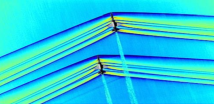
Figure 3.    NASA’s first Schlieren photo of shock waves interacting between two aircrafts taken in March 2019

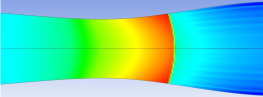
Figure 4. Diagram of a de Laval nozzle for the approximate flow velocity

Figure 5.    Leonhard Euler (15 April 1707 – 18 September 1783) formulated the Euler equations for fluid mechanics which are among the first PDEs to be written down

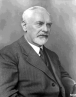
Figure 6. Ludwig Prandtl (4 February 1875 – 15 August 1953) identified two oblique shock configurations when a steady uniform supersonic gas flow passes a solid wedge via the shock polar analysis in 1936

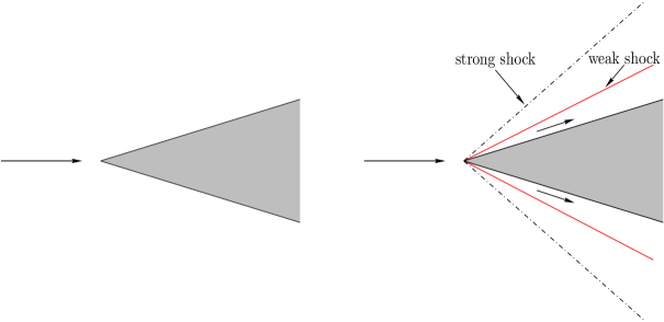
Figure 7. Two steady solutions with shocks around the solid wedge with angle $\theta_{\rm w}\in(0,\theta_{\rm w}^{\rm s})$ or even $\theta_{\rm w}\in[\theta_{\rm w}^{\rm s},\theta_{\rm w}^{\rm d})$

Figure 8. Richard Courant (8 January 1888 – 27 January 1972) and Kurt Otto Friedrichs (28 September 1901 – 31 December 1982); their monumental book [12] has had great impact on the development of the M-D theory of shock waves and nonlinear PDEs of hyperbolic/mixed types

Many fundamental transonic flow problems in fluid mechanics involve these nonlinear PDEs of mixed type. One of them is a classical shock problem, in which an upstream steady uniform supersonic gas flow passes a symmetric straight-sided solid wedge

$$W:=\{\mathbf{x}=(x_{1},x_{2})\in\mathbb{R}^{2}\,:\,|x_{2}|<x_{1}\tan\theta_{\rm w},x_{1}>0\},$$ (2.4)

whose (half-wedge) angle $\theta_{\rm w}$ is less than the detachment angle $\theta^{\rm d}_{\rm w}$ (cf. Fig. 7).

Since this problem involves shocks, its global solution should be a weak solution of equation (2.2) or system (2.3) in the distributional sense (which admit shocks) in the domain under consideration (see [7]). For example, for equation (2.2), a shock is a curve across which $\nabla\varphi$ is discontinuous. If $\Lambda^{+}$ and $\Lambda^{-}(:=\Lambda\setminus\overline{\Lambda^{+}})$ are two nonempty open subsets of a domain $\Lambda\subset\mathbb{R}^{2}$, and $\mathcal{S}:=\partial\Lambda^{+}\cap\Lambda$ is a $C^{1}$-curve across which $\nabla\varphi$ has a jump, then $\varphi\in C^{1}(\Lambda^{\pm}\cup\mathcal{S})\cap C^{2}(\Lambda^{\pm})$ is a global weak solution of (2.2) in $\Lambda$ if and only if $\varphi$ is in $W^{1,\infty}_{\rm loc}(\Lambda)$ and satisfies equation (2.2) and the Rankine-Hugoniot conditions on $\mathcal{S}$:

$$\varphi_{\Lambda^{+}\cap\mathcal{S}}=\varphi_{\Lambda^{-}\cap\mathcal{S}},\qquad\rho_{B}(|\nabla\varphi|^{2})\nabla\varphi\cdot{\bm{\nu}}|_{\Lambda^{+}\cap\mathcal{S}}=\rho_{B}(|\nabla\varphi|^{2})\nabla\varphi\cdot{\bm{\nu}}|_{\Lambda^{-}\cap\mathcal{S}},$$ (2.5)

where ${\bm{\nu}}$ is the unit normal to $\mathcal{S}$ in the flow direction, i.e., $\nabla\varphi\cdot{\bm{\nu}}|_{\Lambda^{\pm}\cap\mathcal{S}}>0$. A piecewise smooth solution with discontinuities satisfying (2.5) is called an entropy solution of (2.2) if it satisfies the entropy condition: the density $\rho$ increases in the flow direction of $\nabla\varphi_{\Lambda^{+}\cap\mathcal{S}}$ across any discontinuity. Then such a discontinuity is called a shock (also see [12]).

For this problem, there are two configurations: the weak oblique shock reflection with supersonic/subsonic downstream flow (determined by the sonic angle $\theta_{\rm w}^{\rm s}$) and the strong oblique shock reflection with subsonic downstream flow – both satisfy the entropy condition, as discovered by Prandtl (cf. Fig. 6). The weak oblique shock is transonic with subsonic downstream flow for $\theta_{\rm w}\in(\theta_{\rm w}^{\rm s},\theta_{\rm w}^{\rm d})$, while the weak oblique shock is supersonic with supersonic downstream flow for $\theta_{\rm w}\in(0,\theta_{\rm w}^{\rm s})$. However, the strong oblique shock is always transonic with subsonic downstream flow. The question of physical admissibility of one or both of the strong/weak shock reflection configurations had been debated over the past eight decades since Courant-Friedrichs [12] and von Neumann [20], and has been better understood only recently (cf. [7] and the references cited therein). Two natural approaches for understanding this phenomenon are to examine whether these configurations are stable under steady perturbations and to determine whether these configurations are attainable as large-time asymptotic states (i.e., the Prandtl-Meyer problem); both approaches involve the analysis of nonlinear PDEs (2.2) or (2.3) of mixed type.

Mathematically, the steady stability problem can be formulated as a free boundary problem with the perturbed shock-front:

$$\mathcal{S}=\{\mathbf{x}\,:\,x_{2}=\sigma(x_{1}),\,x_{1}\geq 0\}\qquad\quad\mbox{with $\sigma(0)=0\,$ and $\sigma(x_{1})>0$ for $x_{1}>0$},$$ (2.6)

as a free boundary (with the Rankine-Hugoniot conditions, say (2.5), as free boundary conditions) to determine the domain behind $\mathcal{S}$:

$$\Omega=\{\mathbf{x}\in\mathbb{R}^{2}\,:\,b(x_{1})<x_{2}<\sigma(x_{1}),x_{1}>0\}.$$ (2.7)

and the downstream flow in $\Omega$ for the nonlinear equation (2.2) or system (2.3) of mixed elliptic-hyperbolic type, where $x_{2}=b(x_{1})$ is the perturbation of the flat wedge boundary $x_{2}=x_{1}\tan\theta_{\rm w}$. Such a global solution of the free boundary problem provides not only the global structural stability of the steady oblique shock, but also a more detailed structure of the solution.

Figure 9. The leading steady shock $x_{2}=\sigma(x_{1})$ as a free boundary under the perturbation

Supersonic (i.e., supersonic-supersonic) shocks correspond to the case when $\theta_{\rm w}\in(0,\theta_{\rm w}^{\rm s})$, which are shocks of weak strength. The local stability of such shocks was first established in the 1960s. The global stability and uniqueness of the supersonic oblique shocks for both equation (2.2) and system (2.3) have been solved for more general perturbations of both the upstream steady flow and the wedge boundary, even in $BV$, by purely hyperbolic methods and techniques (cf. [7] and the references cited therein).

For transonic (i.e., supersonic-subsonic) shocks, it has been proved that the oblique shock of weak strength is always stable under general steady perturbations. However, the oblique shock of strong strength is stable only conditionally for a certain class of steady perturbations that require the exact match of the steady perturbations near the wedge-vertex and the downstream condition at infinity, which reveals one of the reasons why the strong oblique shock solutions have not been observed by experiment. In these stability problems for transonic shocks, the PDEs (or parts of the systems) are expected to be elliptic for global solutions in the domains determined by the corresponding free boundary problems. That is, we solve an expected elliptic free boundary problem. However, the earlier methods and approaches of elliptic free boundary problems do not directly apply to these problems, such as the variational methods, the Harnack inequality approach, and other elliptic methods/approaches. The main reason is that the type of equations needs to be controlled before we can apply these methods, which requires some strong a priori estimates. To overcome these difficulties, the global structure of the problems is exploited, which allows us to derive certain properties of the solution so that the type of equations and the geometry of the problem can be controlled. With this, the free boundary problem as described above has been solved by an iteration procedure. See Chen-Feldman [7] and the references cited therein for more details.

When a subsonic flow passes through a de Laval nozzle, the flow may form a supersonic bubble with a transonic shock (see Fig. 4); the full understanding of how the geometry of the nozzle helps to create/stabilize/destabilize the transonic shock requires a deep understanding of the nonlinear PDEs of mixed type. Likewise, for the Morawetz problem for a steady subsonic flow past an airfoil, experimental results show that a supersonic bubble may be formed around the airfoil (see Figs. 11–11), and the flow behavior is determined by the solution of the nonlinear PDE of mixed type.

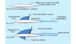
Figure 10. Transonic flow patterns on an airfoil showing flow patterns at and above the critical Mach number

Figure 11. Aerodynamic condensation evidences of supersonic expansion fans around a transonic aircraft

Some fundamental problems for transonic flow posed in the 1950s–60s (e.g., [3, 6, 12, 15, 19]) remain unsolved, though some progress has been made in recent years (e.g., [6, 7, 13] and the references cited therein).

3. Nonlinear PDEs of Mixed Type and Shock Reflection/Diffraction Problems in Fluid Mechanics and Related Areas

In general, fluid flows are time-dependent. We now describe how some longstanding M-D time-dependent fundamental shock problems in fluid mechanics can naturally be formulated as problems for nonlinear PDEs of mixed type, through a prototype – the shock reflection-diffraction problem.

When a planar shock separating two constant states (0) and (1), with constant velocities and densities $\rho_{0}<\rho_{1}$ (state (0) is ahead or to the right of the shock, and state (1) is behind the shock), moves in the flow direction (i.e., $v_{1}>0$) and hits a symmetric wedge (2.4) with (half-wedge) angle $\theta_{\rm w}$ head-on at time $t=0$, a reflection-diffraction process takes place for $t>0$. A fundamental question is which types of wave patterns of shock reflection-diffraction configurations may be formed around the wedge. The complexity of these configurations was first reported by Ernst Mach (cf. Fig. 12), who observed two patterns of shock reflection-diffraction configurations: Regular reflection (two-shock configuration) and Mach reflection (three-shock/one-vortex-sheet configuration), as shown in Fig. 14 below. The issue remained dormant until the 1940s, when John von Neumann [19, 20] (also cf. Fig. 13), as well as other mathematical/experimental scientists (cf. [2, 6, 12, 15] and the references cited therein), began extensive research into all aspects of shock reflection-diffraction phenomena. It has been found that the situations are much more complicated than what Mach originally observed: The shock reflection can be further divided into more specific sub-patterns, and various other patterns of shock reflection-diffraction configurations may occur, such as the supersonic regular reflection, the subsonic regular reflection, the attached regular reflection, the double Mach reflection, the von Neumann reflection, and the Guderley reflection; see [2, 6, 12, 15] and the references cited therein (also see Figs. 14–19 below). Then the fundamental scientific issues include:

• Structures of the shock reflection-diffraction configurations;

• Transition criteria between the different patterns of the configurations;

• Dependence of the patterns upon the physical parameters such as the wedge angle $\theta_{\rm w}$, the incident-shock-wave Mach number (i.e., the strength of the incident shock), and the adiabatic exponent $\gamma>1$.

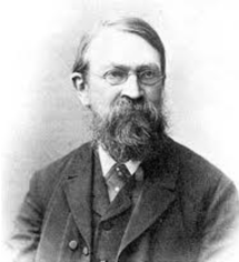
Figure 12.    Ernst Waldfried Josef Wenzel Mach (18 February 1838 – 19 February 1916) who first observed the complexity of shock reflection-diffraction configurations (1878)

Figure 13. John von Neumann (28 December 1903 – 8 February 1957) who proposed the sonic conjecture and the detachment conjecture for shock reflection-diffraction configurations

In particular, several transition criteria between the different patterns of shock reflection-diffraction configurations have been proposed, including the sonic conjecture and the detachment conjecture by von Neumann [19] (also see [2, 6]).

Figure 14. Three patterns of shock reflection-diffraction configurations

To present this more clearly, we focus now on the Euler equations for time-dependent compressible potential flow, which consist of the conservation law of mass and Bernoulli’s law:

$$\partial_{t}\rho+\mbox{div\,}(\rho\,\nabla\Phi)=0,\quad\partial_{t}\Phi+{1\over 2}|\nabla\Phi|^{2}+{1\over\gamma-1}\rho^{\gamma-1}=\frac{\rho_{0}^{\gamma-1}}{\gamma-1}\qquad\quad\,\,\mbox{for $(t,{\bf x})\in{\mathbb{R}}_{+}\times{\mathbb{R}}^{2}$},$$ (3.1)

after scaling, where $\Phi$ is the time-dependent velocity potential (i.e., ${\bm{v}}=\nabla\Phi$ is the velocity). Equivalently, system (3.1) can be reduced to the nonlinear wave equation of second-order:

$${\partial}_{t}{\rho}({\partial}_{t}\Phi,\nabla_{\bf x}\Phi)+\nabla_{\bf x}\cdot\big{(}{\rho}({\partial}_{t}\Phi,\nabla_{\bf x}\Phi)\nabla_{\bf x}\Phi\big{)}=0,$$ (3.2)

with $\rho({\partial}_{t}\Phi,\nabla_{\bf x}\Phi)=\big{(}\rho_{0}^{\gamma-1}-(\gamma-1)({\partial}_{t}\Phi+\frac{1}{2}|\nabla_{\bf x}\Phi|^{2})\big{)}^{\frac{1}{\gamma-1}},$ which is one of the original motivations for the extensive study of nonlinear wave equations.

Mathematically, the shock reflection-diffraction problem is a $2$-D lateral Riemann problem for (3.1) or (3.2) in domain $\mathbb{R}^{2}\setminus\overline{W}$ with $\rho_{0},\rho_{1},v_{1}>0$ satisfying

$$\rho_{1}>\rho_{0},\quad v_{1}=(\rho_{1}-\rho_{0})\sqrt{\frac{2(\rho_{1}^{\gamma-1}-\rho_{0}^{\gamma-1})}{\rho_{1}^{2}-\rho_{0}^{2}}}.$$ (3.3)

Problem 3.1 (Shock Reflection-Diffraction Problem).

Piecewise constant initial data, consisting of state $(0)$ with velocity $\mathbf{v}_{0}=(0,0)$ and density $\rho_{0}>0$ on $\{x_{1}>0\}\setminus\overline{W}$ and state $(1)$ with velocity $\mathbf{v}_{1}=(v_{1},0)$ and density $\rho_{1}>0$ on $\{x_{1}<0\}$ connected by a shock at $x_{1}=0$, are prescribed at $t=0$, satisfying (3.3). Seek a solution of the Euler system (3.1), or Eq. (3.2), for $t\geq 0$ subject to these initial data and the boundary condition $\nabla\Phi\cdot{\bm{\nu}}_{\rm w}=0$ on $\partial W$, where ${\bm{\nu}}_{\rm w}$ is the unit outward normal to $\partial W$.

Problem 3.1 is invariant under scaling: $(t,{\bf x},\Phi)\rightarrow(\tilde{t},\tilde{\bf x},\tilde{\Phi}(\tilde{t},\tilde{\bf x})):=(\alpha t,\alpha{\bf x},\alpha\Phi(t,{\bf x}))$ for any $\alpha\neq 0$, and thus it admits self-similar solutions in the form of

$$\Phi(t,{\bf x})=t\phi({\bm{\xi}})\qquad\quad\text{for}\;\;{\bm{\xi}}=\frac{{\bf x}}{t}.$$ (3.4)

Then the pseudo-potential function $\varphi({\bm{\xi}})=\phi({\bm{\xi}})-\frac{1}{2}|{\bm{\xi}}|^{2}$ satisfies the following equation:

$${\rm div}\big{(}\rho_{B}(|{\rm D}\varphi|^{2},\varphi){\rm D}\varphi\big{)}+2\rho_{B}(|{\rm D}\varphi|^{2},\varphi)=0$$ (3.5)

with $\rho_{B}(|{\rm D}\varphi|,\varphi)=\bigl{(}\rho_{0}^{\gamma-1}-(\gamma-1)(\frac{1}{2}|{\rm D}\varphi|^{2}+\varphi)\bigr{)}^{\frac{1}{\gamma-1}},$ where the divergence ${\rm div}$ and gradient ${\rm D}$ are with respect to ${\bm{\xi}}\in\mathbb{R}^{2}$. Define the pseudo-sonic speed $c=c(|{\rm D}\varphi|,\varphi)$ by

$$c^{2}(|{\rm D}\varphi|,\varphi)=\rho^{\gamma-1}(|{\rm D}\varphi|^{2},\varphi)=B_{0}-(\gamma-1)\big{(}\frac{1}{2}|{\rm D}\varphi|^{2}+\varphi\big{)}.$$ (3.6)

Eq. (3.5) is of mixed elliptic-hyperbolic type – It is

• strictly elliptic if $|{\rm D}\varphi|<c(|{\rm D}\varphi|,\varphi)$ (pseudo-subsonic),

• strictly hyperbolic if $|{\rm D}\varphi|>c(|{\rm D}\varphi|,\varphi)$ (pseudo-supersonic).

The transition boundary between the pseudo-supersonic and pseudo-subsonic phases is $|{\rm D}\varphi|=c(|{\rm D}\varphi|,\varphi)$ (i.e., $|{\rm D}\varphi|=\sqrt{\frac{2}{\gamma+1}\big{(}B_{0}-(\gamma-1)\varphi\big{)}}$ ), a degenerate set of the solution of equation (3.5), which is a priori unknown and more delicate than that of equation (2.2).

One class of solutions of (3.5) is that of constant states that are the solutions with constant velocity $\mathbf{v}_{*}\in\mathbb{R}^{2}$. Then the pseudo-potential of a constant state satisfies ${\rm D}\varphi=\mathbf{v}_{*}-{\bm{\xi}}$ so that

$$\varphi({\bm{\xi}})=-\frac{1}{2}|{\bm{\xi}}|^{2}+\mathbf{v}_{*}\cdot{\bm{\xi}}+C,$$ (3.7)

where $C$ is a constant. For this $\varphi$, the density $\rho$ and sonic speed $c=\rho^{(\gamma-1)/2}$ are positive constants, independent of ${\bm{\xi}}$. Then, from (3.7), the ellipticity condition for the constant state is $|{\bm{\xi}}-\mathbf{v}_{*}|<c.$ Thus, for a constant state $\mathbf{v}_{*}$, equation (3.5) is elliptic inside the sonic circle, with center $\mathbf{v}_{*}$ and radius $c$, and hyperbolic outside this circle. Moreover, if the density $\rho$ is a constant, then the solution is a constant state; that is, the corresponding pseudo-potential $\varphi$ is of form (3.7).

Problem 3.1 involves transonic shocks so that its global solution should be a weak solution of equation (3.5) in the distributional sense within the domain in the ${\bm{\xi}}$–coordinates (see [7]). If $\Lambda^{+}$ and $\Lambda^{-}(:=\Lambda\setminus\overline{\Lambda^{+}})$ are two nonempty open subsets of a domain $\Lambda\subset\mathbb{R}^{2}$, and $\mathcal{S}:=\partial\Lambda^{+}\cap\Lambda$ is a $C^{1}$-curve with normal ${\bm{\nu}}$ across which ${\rm D}\varphi$ has a jump, then $\varphi\in C^{1}(\Lambda^{\pm}\cup\mathcal{S})\cap C^{2}(\Lambda^{\pm})$ is a global entropy solution of (3.5) in $\Lambda$ with $\mathcal{S}$ as a shock if and only if $\varphi$ is in $W^{1,\infty}_{\rm loc}(\Lambda)$ and satisfies equation (3.5), the Rankine-Hugoniot conditions on $\mathcal{S}$:

$$\varphi_{\Lambda^{+}\cap\mathcal{S}}=\varphi_{\Lambda^{-}\cap\mathcal{S}},$$ (3.8)

$$\rho(|{\rm D}\varphi|^{2},\varphi){\rm D}\varphi\cdot{\bm{\nu}}|_{\Lambda^{+}\cap\mathcal{S}}=\rho(|{\rm D}\varphi|^{2},\varphi){\rm D}\varphi\cdot{\bm{\nu}}|_{\Lambda^{-}\cap\mathcal{S}},$$ (3.9)

and the entropy condition: the density $\rho$ increases in the pseudo-flow direction of ${\rm D}\varphi_{\Lambda^{+}\cap\mathcal{S}}$ across any discontinuity.

We now show how such solutions of the nonlinear PDE (3.5) of mixed elliptic-hyperbolic type in self-similar coordinates ${\bm{\xi}}=\frac{{\bf x}}{t}$ can be constructed.

First, by the symmetry of the problem with respect to the $\xi_{1}$–axis, it suffices for us to focus only on the upper half-plane $\{\xi_{2}>0\}$ and prescribe the slip boundary condition: ${\rm D}\varphi\cdot{\bm{\nu}}_{\rm sym}=0$ on the symmetry line $\Gamma_{\rm sym}:=\{\xi_{2}=0\}$ for the interior unit normal ${\bm{\nu}}_{\rm sym}=(0,1)$. Then Problem 3.1 can be reformulated as a boundary value problem in the unbounded domain:

$$\Lambda:=\mathbb{R}^{2}_{+}\setminus\{{\bm{\xi}}\,:\,|\xi_{2}|\leq\xi_{1}\tan\theta_{\rm w},\xi_{1}>0\}$$

in the self-similar coordinates ${\bm{\xi}}=(\xi_{1},\xi_{2})$, where $\mathbb{R}^{2}_{+}:=\mathbb{R}^{2}\cap\{\xi_{2}>0\}$.

Problem 3.2 (Boundary Value Problem).

Seek a solution $\varphi$ of equation (3.5) in the self-similar domain $\Lambda$ with the slip boundary condition: ${\rm D}\varphi\cdot{\bm{\nu}}|_{\partial\Lambda}=0$ for the interior unit normal ${\bm{\nu}}$ on $\partial\Lambda$, and the asymptotic boundary condition at infinity:

$$\varphi\longrightarrow\bar{\varphi}=\begin{cases}\varphi_{0}\qquad\mbox{for}\,\,\,\xi_{1}>\xi_{1}^{0},\xi_{2}>\xi_{1}\tan\theta_{\rm w},\\ \varphi_{1}\qquad\mbox{for}\,\,\,\xi_{1}<\xi_{1}^{0},\;\xi_{2}>0,\end{cases}\qquad\mbox{when $|{\bm{\xi}}|\to\infty$,}$$

where $\varphi_{0}=-\frac{1}{2}|{\bm{\xi}}|^{2}$ and $\varphi_{1}=-\frac{1}{2}|{\bm{\xi}}|^{2}+v_{1}(\xi_{1}-\xi^{0}_{1})$ with $\xi_{1}^{0}=\frac{\rho_{1}v_{1}}{\rho_{1}-\rho_{0}},$ which is the location of the incident shock $\mathcal{S}_{0}=\{\xi_{1}=\xi_{1}^{0}\}\cap\Lambda$ determined by the Rankine-Hugoniot conditions (3.8)–(3.9) between states $(0)$ and $(1)$ on $\mathcal{S}_{0}$.

The simplest case is when $\theta_{\rm w}=\frac{\pi}{2}$, which is called normal reflection; see Fig. 15. In this case, the incident shock normally reflects from the flat wall to become the flat reflected shock $\xi_{1}=\bar{\xi}_{1}<0$.

Figure 15. Normal reflection configuration

When $\theta_{\rm w}\in(0,\frac{\pi}{2})$, a necessary condition for the existence of a regular reflection solution whose configurations are as shown in Figs. 17–19 is the existence of the uniform state (2) with pseudo-potential $\varphi_{2}$ at $P_{0}$, determined by the following three conditions at $P_{0}$:

$${\rm D}\varphi_{2}\cdot{\bm{\nu}}_{\rm w}=0,\,\,\,\,\varphi_{2}=\varphi_{1},\,\,\,\,\rho(|{\rm D}\varphi_{2}|^{2},\varphi_{2}){\rm D}\varphi_{2}\cdot{\bm{\nu}}_{\mathcal{S}_{1}}=\rho_{1}{\rm D}\varphi_{1}\cdot{\bm{\nu}}_{\mathcal{S}_{1}}\qquad\mbox{for ${\bm{\nu}}_{\mathcal{S}_{1}}=\frac{{\rm D}(\varphi_{1}-\varphi_{2})}{|{\rm D}(\varphi_{1}-\varphi_{2})|}$}$$ (3.10)

across the flat shock $\mathcal{S}_{1}=\{\varphi_{1}=\varphi_{2}\}$ that separates state (2) from state (1) and satisfies the entropy condition: $\rho_{2}>\rho_{1}$. These conditions lead to the system of algebraic equations (3.10) for the constant velocity $\mathbf{v}_{2}$ and density $\rho_{2}$ of state (2). For any fixed densities $0<\rho_{0}<\rho_{1}$ of states (0) and (1), there exist a sonic angle $\theta_{\rm w}^{\rm s}$ and a detachment angle $\theta_{\rm w}^{\rm d}$ satisfying

$$0<\theta_{\rm w}^{\rm d}<\theta_{\rm w}^{\rm s}<\frac{\pi}{2}$$

such that the algebraic system (3.10) has two solutions for each $\theta_{\rm w}\in(\theta_{\rm w}^{\rm d},\frac{\pi}{2})$, which become equal when $\theta_{\rm w}=\theta_{\rm w}^{\rm d}$. Thus, for each $\theta_{\rm w}\in(\theta_{\rm w}^{\rm d},\frac{\pi}{2})$, there exist two states (2), called weak and strong, with densities $0<\rho_{1}<\rho_{2}^{\rm weak}<\rho_{2}^{\rm strong}$ (the entropy condition). The weak state (2) is supersonic at the reflection point ${P_{0}}$ for $\theta_{\rm w}\in(\theta_{\rm w}^{\rm s},\frac{\pi}{2})$, sonic for $\theta_{\rm w}=\theta_{\rm w}^{\rm s}$, and subsonic for $\theta_{\rm w}\in(\theta_{\rm w}^{\rm d},\hat{\theta}_{\rm w}^{\rm s})$ for some $\hat{\theta}_{\rm w}^{\rm s}\in(\theta_{\rm w}^{\rm d},\theta_{\rm w}^{\rm s}]$. The strong state (2) is always subsonic at ${P_{0}}$ for all $\theta_{\rm w}\in(\theta_{\rm w}^{\rm d},\frac{\pi}{2})$.

There had been a long debate on determining which of the two states (2) for $\theta_{\rm w}\in(\theta_{\rm w}^{\rm d},\frac{\pi}{2})$, weak or strong, is physical for the local theory; see [2, 7, 12]. Indeed, it has been shown in Chen-Feldman [5, 7] that the weak shock reflection-diffraction configuration tends to the unique normal reflection in Fig. 15, but the strong one does not, when the wedge angle $\theta_{\rm w}$ tends to $\frac{\pi}{2}$. The strength of the corresponding reflected shock near $P_{0}$ in the weak shock reflection-diffraction configuration is relatively weak, compared to the other shock given by the strong state (2). From now on, for the given wedge angle $\theta_{\rm w}\in(\theta_{\rm w}^{\rm d},\frac{\pi}{2})$, state (2) represents the unique weak state (2) and $\varphi_{2}$ is its pseudo-potential.

If the weak state (2) is supersonic, the speeds of propagation of the solution are finite, and state (2) is determined completely by the local information: state (1), state (0), and the location of point $P_{0}$. That is, any information from the reflection-diffraction domain, particularly the disturbance at corner $P_{3}$, cannot travel towards the reflection point $P_{0}$. However, if it is subsonic, the information can reach $P_{0}$ and interact with it, potentially altering the subsonic reflection-diffraction configuration. This argument motivated the following conjectures by von Neumann in [19] (also see [2, 6]):

Figure 16.    Supersonic regular reflection-diffraction configuration [6]

Figure 17.    Subsonic regular reflection-diffraction configuration [6]

The von Neumann Sonic Conjecture: There exists a supersonic regular shock reflection-diffraction configuration when $\theta_{\rm w}\in(\theta_{\rm w}^{\rm s},\frac{\pi}{2})$ for $\theta_{\rm w}^{\rm s}>\theta_{\rm w}^{\rm d}$. That is, the supersonicity of the weak state (2) implies the existence of a supersonic regular reflection solution, as shown in Fig. 17.

Another conjecture is that the global regular shock reflection-diffraction configuration is still possible whenever the local regular reflection at the reflection point is possible:

The von Neumann Detachment Conjecture: There exists a subsonic regular shock reflection-diffraction configuration for any wedge angle $\theta_{\rm w}\in(\theta_{\rm w}^{\rm d},\theta_{\rm w}^{\rm s})$. That is, the existence of subsonic weak state (2) beyond the sonic angle implies the existence of a subsonic regular reflection solution, as shown in Fig. 17.

State (2) determines the straight shock $\mathcal{S}_{1}$ and the sonic arc $\Gamma_{\rm sonic}:=P_{1}P_{4}$ when state (2) is supersonic at $P_{0}$, and the slope of $\Gamma_{\rm shock}$ at $P_{0}$ (arc $\Gamma_{\rm sonic}$ on the boundary of $\Omega$ becomes a corner point $P_{0}$) when state (2) is subsonic at $P_{0}$. Thus, the unknowns are the domain $\Omega$ (or equivalently, the curved part of the reflected-diffracted shock $\Gamma_{\rm shock}$) and the pseudo-potential $\varphi$ in $\Omega$. Then, from (3.8)–(3.9), in order to construct a solution of Problem 3.2 for the supersonic/subsonic regular shock reflection-diffraction configurations, it suffices to solve the following problem:

Problem 3.3 (Free Boundary Problem).

For $\theta_{\rm w}\in(\theta_{\rm w}^{\rm d},\frac{\pi}{2})$, find a free boundary $($curved reflected shock$)$ $\Gamma_{\rm shock}\subset\Lambda\cap\{{\xi_{1}}<\xi_{1{P_{1}}}\}$ ($\Gamma_{\rm shock}=P_{1}P_{2}$ on Fig. 17 and $\Gamma_{\rm shock}=P_{0}P_{2}$ on Fig. 17$)$ and a function $\varphi$ defined in the domain $\Omega$ as shown in Figs. 17–17 such that

• Equation (3.5) is satisfied in $\Omega$, and the equation is strictly elliptic for $\varphi$ in $\overline{\Omega}\setminus\overline{\Gamma}_{\rm sonic}$,

• $\varphi=\varphi_{1}$ and $\rho{\rm D}\varphi\cdot{\bm{\nu}}_{\rm s}=\rho_{1}{\rm D}\varphi_{1}\cdot{\bm{\nu}}_{\rm s}$ on the free boundary $\Gamma_{\rm shock}$,

• $\varphi=\varphi_{2}$ and ${\rm D}\varphi={\rm D}\varphi_{2}$ on $\Gamma_{\rm sonic}$ in the supersonic case as shown in Fig. 17 and at $P_{0}$ in the subsonic case as shown in Fig. 17,

• ${\rm D}\varphi\cdot{\bm{\nu}}_{\rm w}=0$ on $\Gamma_{\rm wedge}=P_{0}P_{3}$, and ${\rm D}\varphi\cdot{\bm{\nu}}_{\rm sym}=0$ on $\Gamma_{\rm sym}$,

where ${\bm{\nu}}_{\rm s}$ is the interior unit normal to $\Omega$ on $\Gamma_{\rm shock}$.

Indeed, if $\varphi$ is a solution of Problem 3.3, we extend $\varphi$ from $\Omega$ to $\Lambda$ to become a global entropy solution (see Figs. 17–17) by defining:

$$\varphi=\begin{cases}\,\varphi_{0}\qquad\,\mbox{for}\,\,\xi_{1}>\xi_{1}^{0}\mbox{ and }\xi_{2}>\xi_{1}\tan\theta_{\rm w},\\ \,\varphi_{1}\qquad\,\mbox{for}\,\,\xi_{1}<\xi_{1}^{0}\mbox{ and above curve}\,\,P_{0}{P_{1}}{P_{2}},\\ \,\varphi_{2}\qquad\,\mbox{in region}\,\,P_{0}{P_{1}}{P_{4}}.\end{cases}$$ (3.11)

For the subsonic reflection case, domain $P_{0}{P_{1}}{P_{4}}$ is one point and curve $P_{0}{P_{1}}{P_{2}}$ is $P_{0}{P_{2}}$. Then the global solutions involve two types of transonic (hyperbolic-elliptic) transition: one is from the hyperbolic to the elliptic phases via $\Gamma_{\rm shock}$; the other is from the hyperbolic to the elliptic phases via $\Gamma_{\rm sonic}$.

The conditions in Problem 3.3(ii) are the Rankine-Hugoniot conditions (3.8)–(3.9) on $\Gamma_{\rm shock}$ between $\varphi_{|\Omega}$ and $\varphi_{1}$. Since $\Gamma_{\rm shock}$ is a free boundary and equation (3.5) is strictly elliptic for $\varphi$ in $\overline{\Omega}\setminus\overline{\Gamma}_{\rm sonic}$, then two conditions — the Dirichlet and oblique derivative conditions — on $\Gamma_{\rm shock}$ are consistent with one-phase free boundary problems for nonlinear elliptic PDEs of second order.

In the supersonic case, the conditions in Problem 3.3(iii) are the Rankine-Hugoniot conditions on $\Gamma_{\rm sonic}$ (weak discontinuity) between $\varphi_{|\Omega}$ and $\varphi_{2}$ so that, if $\varphi$ is a solution of Problem 3.3, its extension by (3.11) is a weak solution of Problem 3.2. Since $\Gamma_{\rm sonic}$ is not a free boundary (its location is fixed), it is impossible in general to prescribe the two conditions given in Problem 3.3(iii) on $\Gamma_{\rm sonic}$ for a second-order elliptic PDE. In the iteration problem, we prescribe the condition: $\varphi=\varphi_{2}$ on $\Gamma_{\rm sonic}$, and then prove that ${\rm D}\varphi={\rm D}\varphi_{2}$ on $\Gamma_{\rm sonic}$ by exploiting the elliptic degeneracy on $\Gamma_{\rm sonic}$.

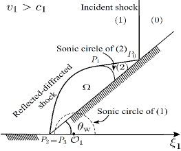
Figure 18. Attached supersonic regular reflection-diffraction configuration

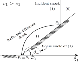
Figure 19. Attached subsonic regular reflection-diffraction configuration

We observe that there is an additional possibility to the regular shock reflection-diffraction configurations (beyond the conjectures by von Neumann [19]): for some wedge angle $\theta_{\rm w}^{\rm a}\in(\theta_{\rm w}^{\rm d},\frac{\pi}{2})$, $\Gamma_{\rm shock}$ may attach to the wedge vertex ${P_{3}}$, as observed by experimental results (cf. [6]); also see Figs. 19–19. To describe the conditions of such an attachment, we use the explicit expressions (3.3) to see that, for each $\rho_{0}$, there exists $\rho^{\rm c}>\rho_{0}$ such that

$$v_{1}\leq c_{1}\quad\mbox{if $\rho_{1}\in(\rho_{0},\rho^{\rm c}]$};\,\qquad\quad v_{1}>c_{1}\quad\mbox{if $\rho_{1}\in(\rho^{\rm c},\infty)$}.$$

If $v_{1}\leq c_{1}$, we can rule out the solution with a shock attached to $P_{3}=(0,0)$. This is based on the fact that, if $v_{1}\leq c_{1}$, then $P_{3}$ lies within the sonic circle $\overline{B_{c_{1}}(\mathbf{v}_{1})}$ of state (1), and $\Gamma_{\rm shock}$ does not intersect $\overline{B_{c_{1}}(\mathbf{v}_{1})}$, as we show below. If $v_{1}>c_{1}$, there would be a possibility that $\Gamma_{\rm shock}$ could be attached to $P_{3}$ as the experiments show. With these, the following results have been obtained:

Theorem 3.4 (Chen-Feldman [5, 6]).

There are two cases:

1. If $\rho_{0}$ and $\rho_{1}$ are such that $v_{1}\leq c_{1}$, then the supersonic/subsonic regular reflection solution exists for each $($half-wedge$)$ angle $\theta_{\rm w}\in(\theta_{\rm w}^{\rm d},\frac{\pi}{2})$. That is, for each $\theta_{\rm w}\in(\theta_{\rm w}^{\rm d},\frac{\pi}{2})$, there exists a solution $\varphi$ of Problem 3.3 such that

   $$\Phi(t,{\bf x})=t\,\varphi(\frac{\bf x}{t})+\frac{|{\bf x}|^{2}}{2t}\qquad\mbox{for}\,\,\frac{\bf x}{t}\in\Lambda,\,t>0,$$

   with $\rho(t,{\bf x})=\big{(}\rho_{0}^{\gamma-1}-(\gamma-1)\big{(}\partial_{t}\Phi+\frac{1}{2}|\nabla_{\bf x}\Phi|^{2}\big{)}\big{)}^{\frac{1}{\gamma-1}}$, is a global weak solution of Problem 3.1 satisfying the entropy condition; that is, $\Phi(t,{\bf x})$ is an entropy solution.

2. If $\rho_{0}$ and $\rho_{1}$ are such that $v_{1}>c_{1}$, then there exists $\theta_{\rm w}^{\rm a}\in[\theta_{\rm w}^{\rm d},\frac{\pi}{2})$ so that the regular reflection solution exists for each angle $\theta_{\rm w}\in(\theta_{\rm w}^{\rm a},\frac{\pi}{2})$, and the solution is of the self-similar structure described in (i) above. Moreover, if $\theta_{\rm w}^{\rm a}>\theta_{\rm w}^{\rm d}$, then, for the wedge angle $\theta_{\rm w}=\theta_{\rm w}^{\rm a}$, there exists an attached solution, i.e., $\varphi$ is a solution of Problem 3.3 with ${P_{2}}={P_{3}}$.

The type of regular shock reflection-diffraction configurations $($supersonic as in Fig. 17 and Fig. 19, or subsonic as in Fig. 17 and Fig. 19$)$ is determined by the type of state (2) at ${P_{0}}$:

1. For the supersonic/sonic reflection case, the reflected-diffracted shock ${P_{0}}{P_{2}}$ is $C^{2,\alpha}$–smooth for some $\alpha\in(0,1)$ and its curved part $\Gamma_{\rm sonic}$ is $C^{\infty}$ away from $P_{1}$. The solution $\varphi$ is in $C^{1,\alpha}(\overline{\Omega})\cap C^{\infty}(\Omega)$, and is $C^{1,1}$ across $\Gamma_{\rm sonic}$ which is optimal; that is, $\varphi$ is not $C^{2}$ across $\Gamma_{\rm sonic}$.

2. For the subsonic reflection case $($as in Fig. 17 and Fig. 19$)$, the reflected-diffracted shock ${P_{0}}{P_{2}}$ and solution $\varphi$ in $\Omega$ are in $C^{1,\alpha}$ near $P_{0}$ and $P_{3}$ for some $\alpha\in(0,1)$, and $C^{\infty}$ away from $\{P_{0},P_{3}\}$.

Moreover, the regular reflection solution tends to the unique normal reflection $($as in Fig. 15) when the wedge angle $\theta_{\rm w}$ tends to $\frac{\pi}{2}$. In addition, for both supersonic and subsonic reflection cases,

$$\varphi_{2}<\varphi<\varphi_{1}\quad\mbox{in $\Omega$},\qquad\quad\,{\rm D}(\varphi_{1}-\varphi)\cdot{\bf e}\leq 0\quad\mbox{in $\overline{\Omega}\,\,$ for all ${\bf e}\in\overline{Cone({\bf e}_{\xi_{2}},{\bf e}_{\mathcal{S}_{1}})}$},$$

where $Cone({\bf e}_{\xi_{2}},{\bf e}_{\mathcal{S}_{1}}):=\{a\,{\bf e}_{\xi_{2}}+b\,{\bf e}_{\mathcal{S}_{1}}\;:\;a,b>0\}$ with ${\bf e}_{\xi_{2}}=(0,1)$ and ${\bf e}_{\mathcal{S}_{1}}$ as the tangent unit vector to $\mathcal{S}_{1}$.

Theorem 3.4 was established by solving Problem 3.3. The first results on the existence of global solutions of the free boundary problem (Problem 3.3) were obtained for the wedge angles sufficiently close to $\frac{\pi}{2}$ in Chen-Feldman [5]. Later, in Chen-Feldman [6], these results were extended up to the detachment angle as stated in Theorem 3.4. For this extension, the techniques developed in [5], notably the estimates near $\Gamma_{\rm sonic}$, were the starting point.

To establish Theorem 3.4, a theory for free boundary problems for nonlinear PDEs of mixed elliptic-hyperbolic type has been developed, including new methods, techniques, and related ideas. Some features of these methods and techniques include:

(i) Exploitation of the global structure of solutions to ensure that the nonlinear PDE (3.5) is elliptic for the regular reflection solution in $\Omega$ enclosed by the free boundary $\Gamma_{\rm shock}$ and the fixed boundary for all wedge angles $\theta_{\rm w}$ up to the detachment angle $\theta_{\rm w}^{\rm d}$ for all the physical cases; see Figs. 16–19.

(ii) Optimal regularity estimates for the solutions of the degenerate elliptic PDE (3.5) both near $\Gamma_{\rm sonic}$ and at corner $P_{1}$ between the free boundary $\Gamma_{\rm shock}$ and the elliptic degenerate fixed boundary $\Gamma_{\rm sonic}$ for the supersonic reflection case; see Fig. 16 and Fig. 18.

(iii) For fixed incident shock strength and $\gamma>1$, the dependence of the structural transition of the global solution configurations on the wedge angle $\theta_{\rm w}$ from the supersonic to subsonic reflection cases, i.e., from the degenerate elliptic to the uniformly elliptic equation (3.5) near a part of the boundary.

(iv) Uniform a priori estimates required for all stages of the structural transition between the different configurations.

Based on these methods and techniques for establishing Theorem 3.4, further approaches and related techniques have been developed to prove that the steady weak oblique transonic shocks, discussed in §2, are attainable as large-time asymptotic states by constructing the global Prandtl-Meyer reflection configurations in self-similar coordinates in Bae-Chen-Feldman [1] and the references cited therein, and that all the self-similar transonic shocks and related free boundaries in these problems are always convex in Chen-Feldman-Xiang [8].

Such questions also arise in other shock reflection/diffraction problems, which can be formulated as free boundary problems for transonic shocks for nonlinear PDEs of mixed type. These problems have the following important attributes: They are physically fundamental and have a wealth of experimental/numerical data indicating diverse patterns of complicated configurations (cf. Figs. 14–19); their solutions are building blocks and asymptotic attractors of general solutions of M-D hyperbolic conservation laws whose mathematical theory is also in its infancy (cf. [2, 6, 13, 15]).

Similarly, for the full Euler case, a self-similar solution is a solution of form: $({\mathbf{V}},p,\rho)(t,{\bf x})=({\bm{v}}-{\bm{\xi}},p,\rho)({\bm{\xi}}),\,{\bm{\xi}}={\bf x}/t$, governed by

$$\begin{cases}\nabla\cdot(\rho{\mathbf{V}})+n\rho=0,\\ \nabla\cdot(\rho{\mathbf{V}}\otimes{\mathbf{V}})+\nabla p+(n+1)\rho{\mathbf{V}}=0,\\ \nabla\cdot\big{(}\rho{\mathbf{V}}(E+\frac{p}{\rho})\big{)}+n\rho(E+\frac{p}{\rho})=0.\end{cases}$$ (3.12)

System (3.12) is a system of conservation laws of mixed-composite elliptic-hyperbolic type – It is

• strictly hyperbolic when $|{\mathbf{V}}|>c:=\sqrt{\gamma p/\rho}$ (pseudo-supersonic),

• mixed-composite elliptic-hyperbolic (two of them are elliptic and the others hyperbolic) when $|{\mathbf{V}}|<c:=\sqrt{\gamma p/\rho}$ (pseudo-subsonic).

The transition boundary between the pseudo-supersonic/pseudo-subsonic phase is $|{\mathbf{V}}|=c$, a degenerate set of the solution of equation (3.12), which is a priori unknown.

Similar fundamental mixed problems arise in other applications, where such nonlinear PDEs of mixed type are the core parts in even more sophisticated systems; for example, the relativistic Euler equations, the Euler-Poisson equations, and the Euler-Maxwell equations.

4. Nonlinear PDEs of Mixed Type and Isometric Embedding Problems in Differential Geometry and Related Areas

Nonlinear PDEs of mixed type also arise naturally from many longstanding problems in differential geometry and related areas. In this section, we first show how the fundamental problem – the isometric embedding problem – in differential geometry can be formulated as problems for nonlinear PDEs of mixed type, or even no type.

The isometric embedding problem can be stated as follows: Seek an embedding/immersion of an $n$-D $($semi-$)$Riemannian manifold $(\mathcal{M}^{n},g)$ with metric $g=(g_{ij})>0$ into an $N$-D $($semi-$)$ Euclidean space so that the metric, often along with assigned regularity/curvatures, is preserved.

This problem has assumed a position of fundamental conceptual importance in differential geometry since the works of Darboux (1894), Weyl (1916), Janet (1926), and Cartan (1927). A classical question is whether a smooth Riemannian manifold $(\mathcal{M}^{n},g)$ can be embedded into $\mathbb{R}^{N}$ with sufficiently large $N$; e.g. Nash (1956), Gromov (1986), and Günther (1989). A further fundamental issue is whether $(\mathcal{M}^{n},g)$ can be embedded/immersed in $\mathbb{R}^{s_{n}}$ with critical Janet dimension $s_{n}=\frac{n(n+1)}{2}$ and assigned regularity/curvatures. The solution to this issue will advance our understanding of properties of (semi-)Riemannian manifolds and provide frameworks/approaches for real applications, including the problems for realization/stability/rigidity/classification of isometric embeddings in many important application areas (see e.g. elasticity, materials science, optimal designs, thin shell/biological leaf growth, protein folding, cell/tissue organization, and manifold data analysis).

When $n=2$, following Darboux, the isometric embedding problem on a chart can be reduced to finding a function $u$ that solves the following nonlinear Monge-Ampère equation (cf. [17]):

$$\qquad\quad\det(\nabla^{2}u)=|g|\big{(}1-|\nabla u|^{2}_{g}\big{)}K,$$ (4.1)

with $|g|=\det(g)$, $|\nabla u|_{g}:=\frac{1}{|g|}\big{(}g_{22}|\partial_{x_{1}}u|^{2}-2g_{12}\partial_{x_{1}}\partial_{x_{2}}u+g_{11}|\partial_{x_{2}}u|^{2}\big{)}<1$ as required, and the Gauss curvature $K=K(g)$ of metric $g$. Equation (4.1) is elliptic if $K>0$, hyperbolic if $K<0$, and degenerate when $K=0$. The sign change of $K$ is very common for surfaces and is necessary for many important cases; the simplest example of such surfaces is the torus as shown in Fig. 21.

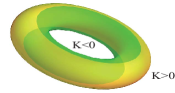
Figure 20.   The Gauss curvature $K$ of a torus with mixed sign

Figure 21. Johann Carl Friedrich Gauss (30 April 1777 – 23 February 1855) introduced the notion of Gauss (or Gaussian) curvature and the Theorema Egregium

Figure 22.    Jean-Gaston Darboux (14 August 1842 – 23 February 1917) indicated the connection between the isometric embedding and the nonlinear Monge-Ampère equation

Figure 23. John Forbes Nash Jr. (13 June 1928 – 23 May 2015) established the Nash embedding theorems

Nirenberg (1953) first solved the Weyl problem, establishing that any smooth metric $g$ on $\mathbb{S}^{2}$ can be globally embedded into $\mathbb{R}^{3}$ smoothly if the Gauss curvature $K>0$. Then one would ask whether any 2-D Riemannian surface is always embeddable into ${\mathbb{R}}^{3}$. The answer is no if $K\leq 0$. The embedding problem is still largely open for global results for general $K$, even though some local results have been obtained; see [17] and the references therein.

On the other hand, the fundamental theorem of surface theory states that there exists a simply connected surface in $\mathbb{R}^{3}$ whose first and second fundamental forms are $I=g_{ij}dx_{i}dx_{j}$ and $I\!I=h_{ij}dx_{i}dx_{j}$ on a domain for $i,j=1,2$, provided that the coefficients $\{h_{ij}\}$, together with metric $g=(g_{ij})>0$, satisfy the Gauss-Codazzi equations:

$$\,\,LN-M^{2}=K,$$ (4.2)

$$\begin{cases}\partial_{x_{1}}{N}-\partial_{x_{2}}{M}=-\Gamma^{1}_{22}L+2\Gamma^{1}_{12}M-\Gamma^{1}_{11}N,\\ \partial_{x_{1}}{M}-\partial_{x_{2}}{L}=\Gamma^{2}_{22}L-2\Gamma^{2}_{12}M+\Gamma^{2}_{11}N,\end{cases}$$ (4.3)

where $L={h_{11}}/{\sqrt{|g|}},M={h_{12}}/{\sqrt{|g|}}$, and $N={h_{22}}/{\sqrt{|g|}}$, and $\Gamma^{k}_{ij}$ are the Christoffel symbols for $i,j,k=1,2$. This theorem still holds for immersion even when $\{h_{ij}\}$ is only in $L^{p}$ for $p>2$. Thus, given $(g_{ij})>0$, system (4.2)–(4.3) consists of three nonlinear PDEs for the unknowns $(L,M,N)$ determining $\{h_{ij}\}$ whose knowledge gives a desired immersion. Then the problem can be reduced to the solvability of system (4.3) under constraint (4.2), which is of mixed elliptic-hyperbolic type determined by the sign of the Gauss curvature $K$. From the viewpoint of geometry, (4.2) is a constraint condition, while (4.3) are compatibility conditions.

System (4.2)–(4.3) has similar features to those in gas dynamics in §2–§3. A natural question is whether it can be written in a gas dynamic formulation to examine underlying interrelated connections. Indeed, a novel observation in Chen-Slemrod-Wang [11] has indicated that this is the case: the Codazzi system (4.3) can be formulated as the familiar nonlinear balance laws of momentum:

$$\vspace{-3pt}\begin{cases}\partial_{x_{1}}(\rho u^{2}+p)+\partial_{x_{2}}(\rho uv)=-\Gamma^{1}_{22}(\rho v^{2}+p)-2\Gamma^{1}_{12}\rho uv-\Gamma^{1}_{11}(\rho u^{2}+p),\\[4.2679pt] \partial_{x_{1}}(\rho uv)+\partial_{x_{2}}(\rho v^{2}+p)=-\Gamma^{2}_{22}(\rho v^{2}+p)-2\Gamma^{2}_{12}\rho uv-\Gamma^{2}_{11}(\rho u^{2}+p),\end{cases}$$ (4.4)

and the Gauss equation (4.2) becomes the Bernoulli relation: $\rho=(q^{2}+K)^{-1/2}$ if $p=-1/\rho$ chosen as the Chaplygin pressure for $q=\sqrt{u^{2}+v^{2}}$. In this case, define the sound speed: $c=\sqrt{p^{\prime}(\rho)}=1/\rho$. Then

• $q<c$ and the flow is subsonic when $K>0$,

• $q>c$ and the flow is supersonic when $K<0$,

• $q=c$ and the flow is sonic when $K=0$.

A weak compactness framework has been introduced and applied for establishing the existence and weak continuity/stability of isometric embeddings in $W^{2,p},p\geq 2$, in [10, 11], which has shown its high potential. In particular, the weak continuity/stability of the Gauss-Codazzi equations (4.2)–(4.3) and isometric immersions of (semi-)Riemannian manifolds, independent of local coordinates, have been established in [9, 10], even for the case $p=2$.

For the higher dimensional case, the Gauss-Codazzi equations for ${\bm{h}}=\{h_{ij}^{a}\}$ are coupled with the Ricci equations for the coefficients ${\bm{\kappa}}=\{\kappa_{lb}^{a}\}$ of the connection form on the normal bundle to become the Gauss-Codazzi-Ricci equations in a local coordinate chart of the manifold:

$$h_{ji}^{a}h_{kl}^{a}-h_{ki}^{a}h_{jl}^{a}=R_{ijkl}\quad\text{(Gauss equations)},$$ (4.5)

$$\partial_{x_{k}}h_{lj}^{a}-\partial_{x_{l}}h_{kj}^{a}=-\Gamma_{lj}^{m}h_{km}^{a}+\Gamma_{kj}^{m}h_{lm}^{a}-\big{(}\kappa_{kb}^{a}h_{lj}^{b}-\kappa_{lb}^{a}h_{kj}^{b}\big{)}\quad\text{(Codazzi equations)},$$ (4.6)

$$\partial_{x_{k}}\kappa_{lb}^{a}-\partial_{x_{l}}\kappa_{kb}^{a}=g^{ij}\big{(}h^{a}_{li}h^{b}_{kj}-h^{a}_{ki}h^{b}_{lj}\big{)}+\kappa_{lc}^{a}\kappa_{kb}^{c}-\kappa_{kc}^{a}\kappa_{lb}^{c}\quad\text{(Ricci equations)},$$ (4.7)

where $\kappa_{kb}^{a}=-\kappa_{ka}^{b}$ are the coefficients of the connection form on the normal bundle, $R_{ijkl}$ is the Riemann curvature tensor, the indices $a,b,c$ run from $1$ to $N$, and $i,j,k,l,m,n$ run from $1$ to $d\geq 3$. System (4.5)–(4.7) has no type, neither purely hyperbolic nor purely elliptic for general Riemann curvature tensor $R_{ijkl}$. Nevertheless, the weak continuity of the nonlinear system (4.5)–(4.7) has been established.

Theorem 4.1 (Chen-Slemrod-Wang [11]).

Let $({\bm{h}}^{\varepsilon},{\bm{\kappa}}^{\varepsilon})$ be a sequence of solutions of the Gauss-Codazzi-Ricci system (4.5)–(4.7), which is uniformly bounded in $L^{p}$ for $p>2$. Then the weak limit vector field $({\bm{h}},{\bm{\kappa}})$ of the sequence $({\bm{h}}^{\varepsilon},{\bm{\kappa}}^{\varepsilon})$ in $L^{p}$ is still a solution to the Gauss-Codazzi-Ricci system (4.5)–(4.7).

The proof is based on our key observation in [11] for the div-curl structure of system (4.5)–(4.7): For fixed $i,j,k,l,a,b,c$,

$$\text{div}\,(\underbrace{\overbrace{0,\cdots,0,h_{li}^{a,{\varepsilon}}}^{k},0,\cdots,-h_{ki}^{a,{\varepsilon}}}_{l},0,\cdots,0)=R_{1}^{{\varepsilon}},\quad\text{curl}\,(h^{b,{\varepsilon}}_{1j},h^{b,{\varepsilon}}_{2j},\cdots,h^{b,{\varepsilon}}_{dj})=R_{2}^{\varepsilon},$$ (4.8)

$$\text{div}\,(\underbrace{\overbrace{0,\cdots,0,\kappa_{lc}^{a,{\varepsilon}}}^{k},0,\cdots,-\kappa_{kc}^{a,{\varepsilon}}}_{l},0,\cdots,0)=R_{3}^{{\varepsilon}},\quad\text{curl}\,(\kappa^{c,{\varepsilon}}_{1b},\kappa^{c,{\varepsilon}}_{2b},\cdots,\kappa^{c,{\varepsilon}}_{db})=R_{4}^{\varepsilon},$$ (4.9)

$$\text{div}\,(\underbrace{\overbrace{0,\cdots,0,h_{lj}^{b,{\varepsilon}}}^{k},0,\cdots,-h_{kj}^{b,{\varepsilon}}}_{l},0,\cdots,0)=R_{5}^{\varepsilon},\quad\text{curl}\,(\kappa^{a,{\varepsilon}}_{1b},\kappa^{a,{\varepsilon}}_{2b},\cdots,\kappa^{a,{\varepsilon}}_{db})=R_{6}^{{\varepsilon}},$$ (4.10)

where $R_{r},r=1,\dots,6$, consist of the three types of nonlinear quadratic terms:

$${h_{li}^{a,{\varepsilon}}h_{kj}^{b,{\varepsilon}}-h_{ki}^{a,{\varepsilon}}h_{lj}^{b,{\varepsilon}}},\quad\kappa_{lc}^{a,{\varepsilon}}\kappa_{kb}^{c,{\varepsilon}}-\kappa_{kc}^{a,{\varepsilon}}\kappa_{lb}^{c,{\varepsilon}},\quad{\kappa_{kb}^{a,{\varepsilon}}h_{lj}^{b,{\varepsilon}}-\kappa_{lb}^{a,{\varepsilon}}h_{kj}^{b,{\varepsilon}}},$$

besides several linear terms involving $({\bm{h}}^{\varepsilon},{\bm{\kappa}}^{\varepsilon})$, while the nonlinear quadratic terms are actually the scalar products of the vector fields given on the left-hand sides of (4.8)–(4.10). Therefore, this div-curl structure fits the following classical div-curl lemma divinely (Murat 1978, Tartar 1979): Let $\Omega\subset\mathbb{R}^{d},d\geq 2,$ be open and bounded. Let $p,q>1$ such that $\frac{1}{p}+\frac{1}{q}=1$. Assume that, for $\varepsilon>0$, two fields $\mathbf{u}^{\varepsilon}\in L^{p}(\Omega;\mathbb{R}^{d})$ and $\mathbf{v}^{\varepsilon}\in L^{q}(\Omega;\mathbb{R}^{d})$ satisfy the following conditions:

1. $\mathbf{u}^{\varepsilon}\rightharpoonup\mathbf{u}$ weakly in $L^{p}(\Omega;\mathbb{R}^{d})$ and $\mathbf{v}^{\varepsilon}\rightharpoonup\mathbf{v}$ weakly in $L^{q}(\Omega;\mathbb{R}^{d})$ as $\varepsilon\to 0$,

2. ${\rm div}\,\mathbf{u}^{\varepsilon}$ are confined in a compact subset of $W^{-1,p}_{\rm loc}(\Omega;\mathbb{R})$,

3. ${\rm curl}\,\mathbf{v}^{\varepsilon}$ are confined in a compact subset of $W^{-1,q}_{\rm loc}(\Omega;\mathbb{R}^{d\times d})$,

where $W^{-1,p}(\Omega;\mathbb{R})$ is the dual space of $W^{1,q}(\Omega;\mathbb{R})$, and vice versa. Then the scalar product of $\mathbf{u}^{\varepsilon}$ and $\mathbf{v}^{\varepsilon}$ are weakly continuous: $\mathbf{u}^{\varepsilon}\cdot\mathbf{v}^{\varepsilon}\longrightarrow\mathbf{u}\cdot\mathbf{v}$ in the sense of distributions.

With this div-curl lemma, the weak continuity result in Theorem 4.1 can be seen as follows: For the uniformly bounded sequence $({\bm{h}}^{\varepsilon},{\bm{\kappa}}^{\varepsilon})$ in $L^{p},p>2$, $R_{r}^{\varepsilon},r=1,\dots,6,$ are uniformly bounded in $L^{p/2}$, which implies that $R_{r}^{\varepsilon},r=1,\dots,6,$ are compact in $W^{-1,q}_{\rm loc}$ for some $q\in(1,2)$. On the other hand, equations (4.8)–(4.10) imply that $R_{r}^{\varepsilon},r=1,\dots,6,$ are uniformly bounded in $W^{-1,p}_{\rm loc}$ for $p>2$. Then the interpolation compactness argument can yield that

$$R_{r}^{\varepsilon},\,\,r=1,\dots,6,\qquad\text{are confined in a compact set in $H^{-1}_{\rm loc}(\Omega)$}.$$

With this, we can employ the div-curl lemma to conclude that

$$({h_{li}^{a,{\varepsilon}}h_{kj}^{b,{\varepsilon}}-h_{ki}^{a,{\varepsilon}}h_{lj}^{b,{\varepsilon}}},\,\kappa_{lc}^{a,{\varepsilon}}\kappa_{kb}^{c,{\varepsilon}}-\kappa_{kc}^{a,{\varepsilon}}\kappa_{lb}^{c,{\varepsilon}},\,{\kappa_{kb}^{a,{\varepsilon}}h_{lj}^{b,{\varepsilon}}-\kappa_{lb}^{a,{\varepsilon}}h_{kj}^{b,{\varepsilon}}})$$

$$\longrightharpoonup({h_{li}^{a}h_{kj}^{b}-h_{ki}^{a}h_{lj}^{b}},\,{\kappa_{lc}^{a}\kappa_{kb}^{c}-\kappa_{kc}^{a}\kappa_{lb}^{c}},\,{\kappa_{kb}^{a}h_{lj}^{b}-\kappa_{lb}^{a}h_{kj}^{b}})$$

in the sense of distributions as $\varepsilon\to 0$. Then Theorem 4.1 follows.

This local weak continuity result can be extended to the global weak continuity of the Gauss-Codazzi-Ricci system (4.5)–(4.7):

Theorem 4.2 (Chen-Li [10]).

Let $(M,g)$ be a Riemannian manifold with $g\in W^{1,p}$ for $p>2$. Let $({\bm{h}}^{\varepsilon},{\bm{\kappa}}^{\varepsilon})$ be a sequence of solutions $($i.e., the coefficients of the second fundamental form and the connection form on the normal bundle$)$ in $L^{p}$ of the Gauss-Codazzi-Ricci system (4.5)–(4.7) in the distributional sense. Assume that, for any submanifold $K\Subset M$, there exists $C_{K}>0$ independent of ${\varepsilon}$ such that

$$\sup_{\epsilon>0}\|({\bm{h}}^{\varepsilon},{\bm{\kappa}}^{{\varepsilon}})\|_{L^{p}(K)}\leq C_{K}.$$

Then, when ${\varepsilon}\to 0$, there exists a subsequence of $({\bm{h}}^{\varepsilon},{\bm{\kappa}}^{\varepsilon})$ that converges weakly in $L^{p}$ to a pair $({\bm{h}},{\bm{\kappa}})$ that is still a weak solution of the Gauss-Codazzi-Ricci system (4.5)–(4.7).

The proof is based on a compensated compactness theorem in Banach spaces, which leads directly to a globally intrinsic div-curl lemma on Riemannian manifolds, developed in Chen-Li [10]. From the viewpoint of geometry, the $L^{p}$ bounded requirement on the connection form on the normal bundle ${\bm{\kappa}}^{{\varepsilon}}$ is not intrinsic. Therefore, Theorem 4.2 has been reformulated in the following theorem:

Theorem 4.3 (Chen-Giron [9]).

Let $(M,g)$ be a Riemannian manifold with $g\in W^{1,p}$ for $p>2$. Let $({\bm{h}}^{\varepsilon},{\bm{\kappa}}^{\varepsilon})$ be a sequence of solutions $($i.e., the coefficients of the second fundamental form and the connection form on the normal bundle$)$ in $L^{p}$ of the Gauss-Codazzi-Ricci system (4.5)–(4.7) in the distributional sense. Assume that, for any submanifold $K\Subset M$, there exists $C_{K}>0$ independent of ${\varepsilon}$ such that

$$\sup_{\epsilon>0}\|{\bm{h}}^{\varepsilon}\|_{L^{p}(K)}\leq C_{K}.$$

Then there exists a refined sequence $(\tilde{\bm{h}}^{\varepsilon},\tilde{\bm{\kappa}}^{\varepsilon})$, each of which is still a weak solution of the Gauss-Codazzi-Ricci system (4.5)–(4.7), such that, when ${\varepsilon}\to 0$, $(\tilde{\bm{h}}^{\varepsilon},\tilde{\bm{\kappa}}^{\varepsilon})$ converges weakly in $L^{p}$ to a pair $({\bm{h}},{\bm{\kappa}})$ that is still a weak solution of the Gauss-Codazzi-Ricci system (4.5)–(4.7).

As a direct corollary, the weak limit of isometrically immersed surfaces with lower regularity in $W^{2,p}$ is still an isometrically immersed surface in $\mathbb{R}^{d}$ governed by the Gauss-Codazzi-Ricci system (4.5)–(4.7) for any $R_{ijkl}$ (without sign/type restriction) with respect only to the coefficients of the second fundamental form. The weak continuity result in Theorem 4.3 is global and intrinsic, independent of local coordinates, with no restriction on the Riemann curvatures and the types of system (4.5)–(4.7). The key to the proof is to exploit the invariance for a choice of suitable gauge to control the full connection form and to develop a non-abelian div-curl lemma on Riemannian manifolds (see Chen-Giron [9]).

This approach and related observations have been motivated by the theory of polyconvexity in nonlinear elasticity, intrinsic methods in elasticity and nonlinear Korn inequalities, Uhlenbeck compactness and Gauge theory^,, among other ideas.

5. Further Connections, Unified Approaches, and Current Trends

In §2–§4, we have presented several important sets of nonlinear PDEs of mixed elliptic-hyperbolic type, or even no type, in shock wave problems in fluid mechanics and isometric embedding problems in differential geometry and related areas. Such nonlinear PDEs of mixed type arise naturally in other problems in fluid mechanics, differential geometry/topology, nonlinear elasticity, materials science, mathematical physics, dynamical systems, and related areas.

We have shown that free boundary methods, weak convergence methods, and related techniques are useful as unified approaches to deal with the nonlinear mixed problems involving both elliptic and hyperbolic phases in §2–§4. Friedrichs’s positive symmetric techniques have also shown high potential in solving mixed-type problems. Entropy methods and kinetic methods have been useful for solving nonlinear PDEs of hyperbolic or mixed hyperbolic-parabolic type. Variational approaches deserve to be further explored, especially for handling transonic flow problems since the solutions of these problems are critical points of the corresponding functionals. Some approximate methods such as viscosity methods, relaxation methods, shock capturing methods, stochastic methods, and related numerical methods should be further analyzed/developed, and numerical calculations/simulations should also be performed to gain new ideas and motivations. These methods, along with energy estimate techniques, functional analytical methods, measure-theoretic techniques (esp. divergence-measure fields), and other methods, should be further developed into more powerful approaches, applicable to wider classes of nonlinear PDEs of mixed type. The underlying structures of the nonlinear PDEs of mixed type under consideration have been one of our motivating factors in developing new methods/techniques/ideas for unified approaches. As indicated earlier, the analysis of nonlinear PDEs of mixed type is still in its early stages and most nonlinear mixed-type problems are widely open, requiring additional new ideas, methods, and techniques.

Acknowledgements. The author would like to thank his collaborators and former students, including Myoungjean Bae, Jun Chen, Jeanne Clelland, Mikhail Feldman, Tristin Giron, Siran Li, Marshall Slemrod, Dehua Wang, Wei Xiang, and Deane Yang, as well as the colleagues whose work should be cited (but could not be done so as he wished, due to the strict limitation of the reference number and the length by the journal; please see the references cited in [1]–[20]), for their explicit and implicit contributions to the material presented in this article. The research of Gui-Qiang G. Chen was supported in part by the UK Engineering and Physical Sciences Research Council Award EP/L015811/1, EP/V008854, and EP/V051121/1.

References

- [1] Bae, M., Chen, G.-Q., Feldman, M.: Prandtl-Meyer Reflection Configurations, Transonic Shocks, and Free Boundary Problems, Research Monograph, 118 pages, Memoirs of Amer. Math. Soc., AMS: Providence, RI, 2022 (to appear).
- [2] Ben-Dor, G.: Shock Wave Reflection Phenomena, Springer-Verlag: New York, 1991.
- [3] Bers, L.: Mathematical Aspects of Subsonic and Transonic Gas Dynamics, John Wiley & Sons, Inc.: New York, 1958.
- [4] Bitsadze, A. V.: Equations of the Mixed Type, Macmillan Company: New York, 1964.
- [5] Chen, G.-Q., Feldman, M.: Global solutions to shock reflection by large-angle wedges for potential flow, Ann. of Math. 171 (2010), 1019–1134.
- [6] Chen, G.-Q., Feldman, M.: Mathematics of Shock Reflection-Diffraction and von Neumann’s Conjecture. Research Monograph, Annals of Mathematics Studies, 197, Princeton University Press, Princeton, 2018.
- [7] Chen, G.-Q., Feldman, M.: Multidimensional transonic shock waves and free boundary problems, Bulletin of Mathematical Sciences 12(01), 2230002
- [8] Chen, G.-Q., Feldman, M., Xiang, W.: Convexity of self-similar transonic shock waves for potential flow, Arch. Ration. Mech. Anal. 238 (2020), 47–124.
- [9] Chen, G.-Q., Giron, T.: Weak continuity of Gauss-Codazzi-Ricci equations with -bounded second fundamental form, Preprint, 2022 (to be posted at arXiv).
- [10] Chen, G.-Q., Li, S.: Global weak rigidity of the Gauss-Codazzi-Ricci equations and isometric immersions of Riemannian manifolds with lower regularity, J. Geom. Anal. 28(3) (2018), 1957–2007.
- [11] Chen, G.-Q., Slemrod, M., Wang, D.-H.: Isometric embedding and compensated compactness, CMP. 294 (2010), 411–437; Weak continuity of the Gauss-Codazzi-Ricci system for isometric embedding, Proc. Amer. Math. Soc. 138 (2010), 1843–1852.
- [12] Courant, R., Friedrichs, K. O.: Supersonic Flow and Shock Waves, Springer-Verlag: New York, 1948.
- [13] Dafermos, C. M.: Hyperbolic Conservation Laws in Continuum Physics, 4th Ed., Springer-Verlag: Berlin, 2016.
- [14] Evans, L. C.: Partial Differential Equations. Second edition. Graduate Studies in Mathematics, 19. American Mathematical Society: Providence, RI, 2010.
- [15] Glimm, J., Majda, A.: Multidimensional Hyperbolic Problems and Computations, Springer-Verlag: NY, 1991.
- [16] Hadamard, J.: Lectures on Cauchy’s Problem in Linear Partial Differential Equations. Yale University Press: New York, 1923; Dover Publications, New York, 1953.
- [17] Han, Q. and Hong, J.-X.: Isometric Embedding of Riemannian Manifolds in Euclidean Spaces, AMS, RI, 2006.
- [18] Morawetz, C. S.: On a weak solution for a transonic flow problem, Comm. Pure Appl. Math. 38: 797–818, 1985.
- [19] von Neumann, J.: Oblique reflection of shocks, Explo. Res. Rep. 12, Navy Department, Bureau of Ordnance, Washington, DC, 1943; Refraction, intersection, and reflection of shock waves, NAVORD Rep. 203-45, Navy Department, Bureau of Ordnance, Washington, DC, 1945; Collected Works, Vol 6, Pergamon Press, 1963.
- [20] von Neumann, J.: Discussion on the existence and uniqueness or multiplicity of solutions of the aerodynamical equation [Reprinted from MR0044302] (1949), Bull. Amer. Math. Soc. (N.S.), 47 (2010), 145–154.