The ultraviolet C II lines as a diagnostic of $\kappa$-distributed electrons in planetary nebulae

Abstract

Non-Maxwellian $\kappa$ electron energy distributions (EEDs) have been proposed in recent years to resolve the so-called “electron temperature and abundance discrepancy problem” in the study of planetary nebulae (PNe). Thus the need to develop diagnostic tools to determine from observations the EED of PNe is raised. Arising from high energy levels, the ultraviolet (UV) emission lines from PNe present intensities that depend sensitively on the high-energy tail of the EED. In this work, we investigate the feasibility of using the C II]$\lambda$2326/C II$\lambda$1335 intensity ratios as a diagnostic of the deviation of the EED from the Maxwellian distribution (as represented by the $\kappa$ index). We use a Maxwellian decomposition approach to derive the theoretical $\kappa$-EED-based collisionally excited coefficients of C II, and then compute the C II UV intensity ratio as a function of the $\kappa$ index. We analyze the archival spectra acquired by the International Ultraviolet Explorer and measure the intensities of C II UV lines from 12 PNe. By comparing the observed line ratios and the theoretical predictions, we can infer their $\kappa$ values. With the Maxwellian-EED hypothesis, the observed C II]$\lambda$2326/C II$\lambda$1335 ratios are found to be generally lower than those predicted from the observed optical spectra. This discrepancy can be explained in terms of the $\kappa$ EED. Our results show that the $\kappa$ values inferred range from 15 to infinity, suggesting a mild or modest deviation from the Maxwellian distribution. However, the $\kappa$-distributed electrons are unlikely to exist throughout the whole nebulae. A toy model shows that if just about 1–5 percent of the free electrons in a PN had a $\kappa$-EED as small as $\kappa=3$, it would be sufficient to account for the observations.

1 Introduction

Photoionized gaseous nebulae, including planetary nebulae (PNe) and H II regions, serve as a vital probe of the chemical evolution of galaxies and as a natural laboratory for understanding the plasma physics found in extreme physical environments. Extensive observational studies of nebulae have revealed stark differences between the electron temperatures and elemental abundances derived from collisionally excited lines (hereafter CELs) and those derived from recombination spectra, which is often called the “electron temperature and abundance discrepancy problem” (e.g., Peimbert, 1967; Liu et al., 2000; Zhang et al., 2004; García-Rojas et al., 2017). Several alternative solutions have been previously proposed and continue to be hotly debated (see e.g., Danehkar, 2021; Hajduk et al., 2021; García-Rojas et al., 2022; Ruiz-Escobedo & Peña, 2022, as examples of the recent contributions to this debate). Two mechanisms often cited are temperature fluctuations (characterized by the $t^{2}$ temperature fluctuation parameter) and the two-component model consisting of hydrogen-deficient clumps distributed within a diffuse nebula.

Recently, a new promising scenario has been presented for solving the problem. The determinations of nebular temperatures and abundances in most published literature are based on a fundamental but insufficiently demonstrated assumption that the electron energy distribution (hereafter EED) necessarily follows a Maxwell-Boltzmann (hereafter MB) energy distribution. If the EED was indeed non-thermal, the inconsistencies of current plasma diagnostics would be essentially resolved (Nicholls et al., 2012, 2013; Dopita et al., 2013), in which case the EED becomes characterized by a $\kappa$ function where a lower $\kappa$ index corresponds to a larger departure from the MB distribution. Despite the plausibility of this solution, the mechanism for energizing non-thermal electrons is so far unknown. Much of the criticism to the $\kappa$-EED hypothesis is from a theoretical perspective. Given the relatively short relaxation timescale of non-thermal electrons, the photoionization process of gaseous nebulae is expected not to generate a $\kappa$ EED (Ferland et al., 2016; Draine & Kreisch, 2018), casting serious doubt on this hypothesis. Nevertheless, it is premature to conclude that the currently proposed alternative scenarios are necessarily valid. For instance, if the hypothesis of temperature fluctuations held, the $t^{2}$ values required to explain the observations would be too large to be reproduced by canonical photoionization models. Regarding the two-component model, the proposed but unconfirmed hydrogen-deficient inclusions are also of unknown origin.

The $\kappa$ distribution was first introduced to provide an empirical fit to the energy distribution of the earth’s magnetospheric plasma (Vasyliunas, 1968), and was then found to be a natural consequence of the Tsallis statistical mechanics (Livadiotis & McComas, 2009). It has been widely found to be present in the solar wind (Pierrard & Lazar, 2010), in the heliosheath (Livadiotis & McComas, 2011), and the solar corona (Nicolaou et al., 2018). The proposed origin for particle acceleration, such as magnetic reconnection, is a hot topic in space plasma research. It is not unreasonable to speculate that such processes may also affect the EED of PNe, where the “electron temperature and abundance discrepancy problem” is more prominent than observed in H II regions.

Spectral observations may allow us to confirm or refute the presence of the $\kappa$ EED in PNe. The C II dielectronic recombination lines and the continuum emission spectra near the Balmer jump (hereafter BJ) have been proposed to determine the EED (Storey & Sochi, 2013, 2014; Zhang et al., 2014). However, primarily due to large uncertainties, these results are inconclusive or even conflicting. Zhang et al. (2016) determined the $\kappa$ index for a sample of PNe by comparing the CEL ratios and BJ intensities, which appears to not correlate with the other properties of PNe. Lin & Zhang (2020) found that the introduction of the $\kappa$ EED can bring in line the intensity ratios of the O II recombination lines and those predicted by [O III] CEL observations, but the inferred $\kappa$ values are not in agreement with those obtained from comparison of the CEL and BJ intensities. Such studies based on optical spectroscopy suggest that the non-thermal electrons are unlikely to be uniformly distributed across the whole nebulae, but they cannot exclude their presence on a small spatial scale as is found to be the case for the solar system plasma.

The non-thermal high-energy tail of the $\kappa$ EED would cause a stronger impact on the excitation of the ultraviolet (UV) emission lines than on the optical lines. Therefore, UV line fluxes can in principle serve as an excellent probe of the EED in PNe. Based on the observed C II UV line ratios, Humphrey & Binette (2014) and Morais et al. (2021) found evidences supporting the existence of the $\kappa$ EED in Type 2 Active Galactic Nuclei (AGNs), the high-energy analogue of PNe.

In this paper, we investigate the impact of the $\kappa$ EED on the C II]$\lambda$2326/C II$\lambda$1335 line ratios, aiming at examining whether the UV observations indicate the presence of $\kappa$-EED in PNe. Section 2 describes the archival data we will be using. Section 3 describes the method used to derive the C II UV line ratio under a $\kappa$ EED. The results are presented in Section 4 and are discussed in Section 5. Section 6 summarizes the conclusions.

2 Sample and observational data

The UV observations of PNe have been obtained from the International Ultraviolet Explorer (IUE). We extracted the low-resolution spectra obtained with the Short Wavelength Prime (SWP) and Long Wavelength Prime/Long Wavelength Redundant (LWP/LWR) cameras from the INES (IUE Newly Extracted Spectra) Archive. The SWP and LWP/LWR spectra cover the following wavelength ranges: 1150–1980 and 1850–3350 Å, which therefore include the C II$\lambda$1335 and C II]$\lambda$2326 lines, respectively. For the sample selection, we focused on the PNe studied by Zhang et al. (2016) for the sake of comparison. Due to the severe extinction at UV wavelengths, The C II UV lines for most of the PNe are faint or invisible. Discarding those nebulae with only one of the C II lines being detected, we selected the PNe which possess a reasonably good signal-to-noise ratios. In order to ascertain whether the observed features are indeed C II lines rather than glitches or other contaminations, we carefully compared the widths and peak velocities of the two features in each PN, and excluded those with apparent inconsistencies. Finally, we ended with the 12 PNe listed in Table 1. These PNe are ionized bounded and show relatively high electron temperatures, which are the physical conditions favoring the emission of C II UV CELs. All IUE observations were taken with a large aperture of $10\arcsec\times 23\arcsec$ except for two PNe. For NGC 6572, the LWR spectrum obtained with the small aperture ($3\arcsec$ diameter) was used. We did not attempt to make an aperture correction since NGC 6572 is a compact young PN. For NGC 3918, both spectra were obtained using the smaller aperture.

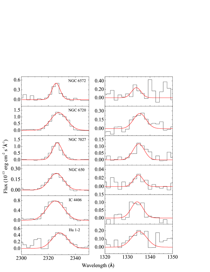
Figure 1: – continued

We subtracted the continuum emission from the IUE spectra by performing a linear fit to the line-free spectral regions. The fluxes of the two C II lines were measured using the Gaussian line profile fitting. Figure 1 shows the IUE spectra and the line fittings for the 12 PNe. The integrated fluxes $F(\lambda)$ were then deredened to derive the intensities by $I(\lambda)$ = 10^c(Hβ)f(λ) $F(\lambda$), where $c({\rm H}\beta)$ is the logarithmic extinction constant taken from Cahn et al. (1992), and $f(\lambda)$ is the standard Galactic extinction law with $R_{V}=3.1$ (Howarth, 1983). See Table 1 for the details.

3 Methodology

Nicholls et al. (2012) for the first time introduced the $\kappa$ function to describe the EED of PNe, which consists of a cold MB-like core characterized by a MB temperature of $T_{c}$ and a power-law superthermal tail,

$$f_{\kappa}(E,T_{U},\kappa)=\frac{2}{\sqrt{\pi}}\frac{\Gamma(\kappa+1)\sqrt{E}}{(k_{B}T_{U})^{1.5}(\kappa-1.5)^{1.5}\Gamma(\kappa-0.5)}\left[1+\frac{E}{(\kappa-1.5)k_{B}T_{U}}\right]^{-\kappa-1}\,,$$ (1)

where $E$, $k_{B}$ and $\Gamma$ are the electron energy, Boltzmann constant, and the Gamma function, respectively. The dimensionless $\kappa$ index ranges from $1.5$ to $\infty$. $T_{U}$ is the nonequilibrium temperature representing the mean kinetic energy of free electrons, which satisfies the relation

$$T_{U}=\frac{\kappa}{\kappa-1.5}T_{c}\,.$$ (2)

When $\kappa\to\infty$, the formula decays to a MB form with $T_{U}=T_{c}$.

The theoretical intensity ratios of C II CELs can be computed by solving the ten energy level balance equation. For that purpose, the collisionally excited rate coefficients ($q$) between any two energy levels are derived from the energy-dependent collision cross sections, $\sigma(E)$, integrated over the EED function. This means

$$q_{M}(T_{M})=\int\sigma(E)\sqrt{E}f_{M}(E,T_{M})dE$$ (3)

under the MB-EED hypothesis (hereafter, we use the subscripts ‘$M$’ and ‘$\kappa$’ to distinguish between the cases under the MB or the $\kappa$ EED assumption, respectively). The tabulated $q_{M}(T_{M})$ values are available in Blum & Pradhan (1992). In principle, $q_{\kappa}(T_{U},\kappa)$ could be obtained by substituting $f_{\kappa}(E,T_{U},\kappa)$ for $f_{M}(E,T)$ in Equ. 3, but such procedure is impractical because numerical evaluation of $\sigma(E)$ is not available from the literature. Hahn & Savin (2015) proposed an easier approach to determine $q_{\kappa}(T_{U},\kappa)$ using the tabulated $q_{M}(T_{M})$. The $\kappa$ function can be mathematically decomposed into several weighted MB functions,

$$f_{\kappa}(E,T_{U},\kappa)=\sum_{j}c_{j}(\kappa)f_{M}(E,T_{M,j})$$ (4)

with $T_{M,j}=a_{j}T_{U}$, where $a_{j}$ and the weighting factor $c_{j}$ are independent of $T_{U}$. Equs. 3 and 4 indicate that

$$q_{\kappa}(T_{U},\kappa)=\sum_{j}c_{j}(\kappa)q_{M}(T_{M,j})\,.$$ (5)

Therefore, we can obtain $q_{\kappa}(T_{U},\kappa)$ by using the above formula and the $a_{j}$, $c_{j}$, and $q_{M}(T_{M})$ values provided by Hahn & Savin (2015) and Blum & Pradhan (1992). This approach for instance has been successfully employed to develop diagnostics for the solar plasma (Dzifčáková et al., 2021). Dzifčáková et al. (2021) noted that this approach provides highly precise results with an uncertainty comparable to the typical uncertainty inherent in the atomic calculations.

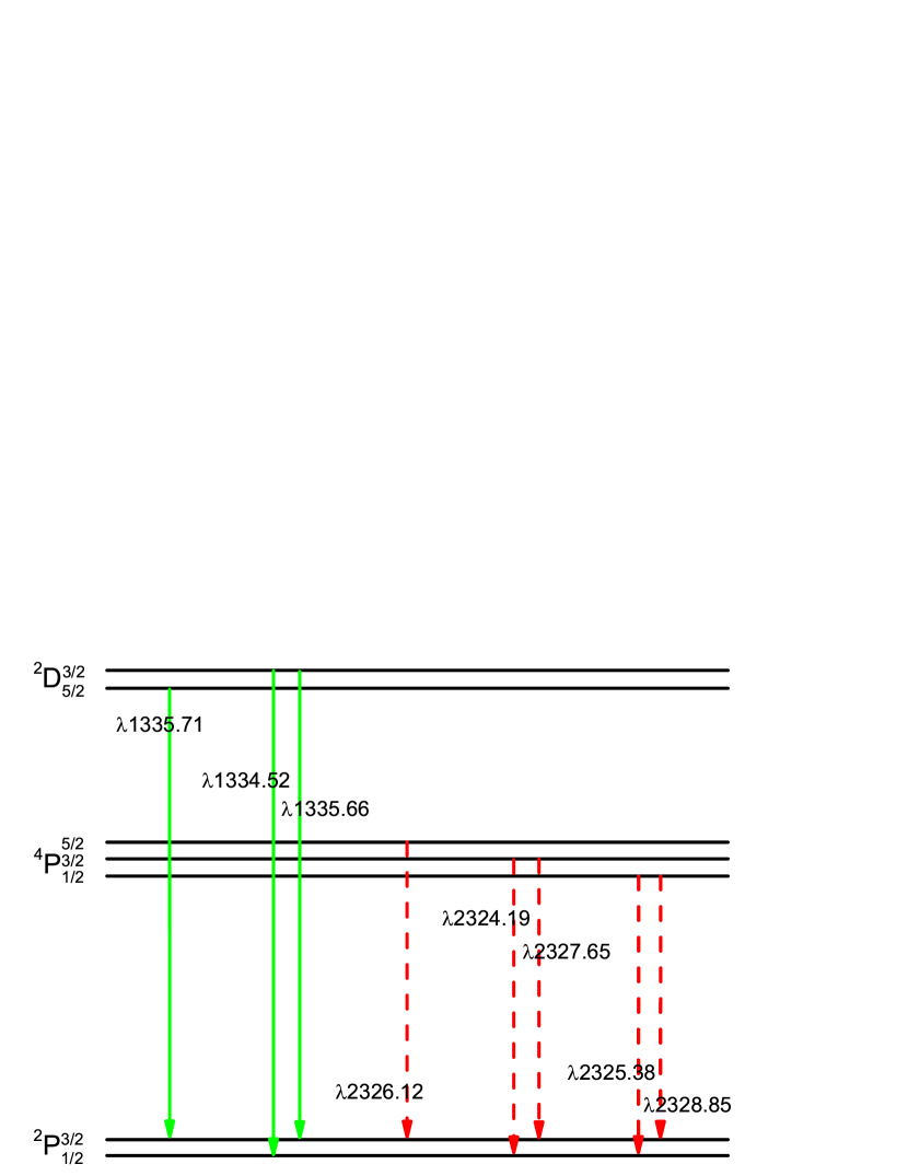
Figure 2: Configuration of the energy levels and transitions of the C II ion.

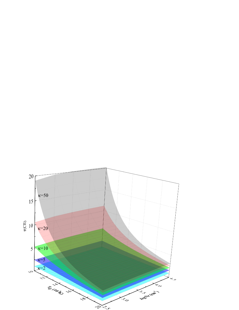
Figure 3: The theoretical C II line ratio as a function of $T_{U}$ and $N_{e}$ for different $\kappa$ values.

The lowest seven levels of C⁺ relevant to the C II UV lines are sketched in Figure 2. As shown in this figure, the $\lambda 1335$ and $\lambda 2326$ features are respectively composed of three and five blended lines that cannot be resolved with IUE spectra. In this work, we will focus on the intensity ratios between the ⁴P_5/2–²P_3/2 transition at 2326.12 Å and the ²D_3/2–²P_1/2 transition at 1334.52 Å, which is hereafter called $r$(C II), in short. Figure 3 shows $r$(C II) as a function of both $T_{U}$ and electron density ($N_{e}$) at various $\kappa$ values. It is conceivable that $r$(C II) decreases with increasing $T_{U}$ and decreasing $\kappa$, which means that higher-energy electrons enhance the $\lambda 1334.52$ line to a larger degree than the $\lambda 2326.12$ line. An inspection of this figure also suggests that $r$(C II) is essentially independent of $N_{e}$. This is because the two lines have critical densities much higher than the typical density found in PNe. At a temperature of $10^{4}$ K, the $\lambda 2326.12$ and $\lambda 1334.52$ lines show a critical density of $7.3\times 10^{8}$ cm^-3 and $2.2\times 10^{15}$ cm^-3, respectively. Consequently, once $T_{U}$ is known, we can infer the $\kappa$ index from the observed $r$(C II). At lower $T_{U}$, $r$(C II) is more sensitive to $\kappa$.

The observed $r$(C II) can be derived by considering the theoretical relative intensities between the blended lines. The $\lambda 1334.52$ and $\lambda 1335.66$ lines arise from the same upper level, and thus their intensity ratio is strictly equal to 5.1, while $I(\lambda 1335.71)$ is about $1.8\times I(\lambda 1334.52)$. It follows that the $\lambda 1334.52$ line has an intensity of 0.34 times that of the blended feature. The $\lambda 2326.12$ line is the strongest among the five blended lines, with an intensity of 0.50 times that of the whole blended feature. These relative intensity ratios are extremely insensitive to the nebular physical conditions in the sense that the blended lines arise from the upper levels with very similar excitation energies and high critical densities ($>10^{7}$ cm^-3). After deblending the C II $\lambda 1335$ and $\lambda 2326$ features, the observed $r$(C II) are derived and their values are listed in the 7th column of Table 1.

4 Results

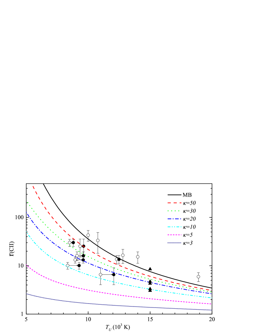
Figure 4: The C II]$\lambda$2326/C II$\lambda$1335 line intensity ratio vs $T_{U}$ for $N_{e}=1000$ cm^-3. The curves indicate the theoretical predictions for various $\kappa$ values, among which the solid line represents the $\kappa=\infty$ case (i.e. the MB distribution). The circles with error bars are the observed values in PNe, where the open and filled circles represent $T_{M}$(BJ) and the derived $T_{U}$ (see text), respectively. The filled triangles denote the observed values in quasars extracted from Vernet et al. (2001), where we have assumed $T_{U}\equiv 1.5\times 10^{4}$ K.

The theoretical and observed $r$(C II) values are compared in Figure 4, where we simply assume $N_{e}=10^{3}$ cm^-3. For that we have derived the $T_{U}$ based on the BJ temperatures, $T_{M}$(BJ), given in the literature (see the 9th column of Table 1). Because the BJ mostly ‘sees’ the cold MB core of the $\kappa$ EED, it is a good approximate to assume $T_{c}=T_{M}({\rm BJ})$. Then $\kappa$ and $T_{U}$ can be iteratively determined from $r$(C II) and Equ. 2. Their values are presented in the 11th and 13th columns of Table 1. The uncertainties of $\kappa$ are found to increase with increasing $T_{U}$ and $\kappa$.

If the EED obeyed the MB distribution, the data points would overlay the $\kappa=\infty$ curve in Figure 4. On the contrary, if the free elections got closer to the $\kappa$ EED with a smaller $\kappa$ index, the CEL with a higher excitation energy would be relatively enhanced, and thus $r$(C II) would decrease and $T_{M}({\rm BJ})$ would be lower than $T_{U}$, meaning that the data points would shift towards the left and down in this figure. We found this to be the case for most of the PNe of our sample, thus providing us a favorable evidence for the $\kappa$ EED in PNe. We could derive well constrained $\kappa$ values for six PNe. NGC 6572 shows a low $\kappa$ index of 17. However, the small-aperture of its LWR spectrum may have caused an underestimation of the C II]$\lambda 2326$ line flux, and thus likely resulted in an underestimation of the $\kappa$ index. The medium $\kappa$ value for the PN sample turns out to be larger than 50, suggesting that most PNe exhibit only mild to modest deviations from the MB distribution.

Humphrey & Binette (2014) found that the $r$(C II) ratio in their AGN sample suggests the presence of a $\kappa$ EED. We reexamined their results in Figure 4 using the observational data retrieved from Vernet et al. (2001), where we have assumed a typical electron temperature of $1.5\times 10^{4}$ K (Osterbrock & Ferland, 2005). Most AGNs exhibit a prominent $\kappa$ EED unless they have an abnormally high temperature, in agreement with the conclusion of Humphrey & Binette (2014). Figure 4 shows that the medium $\kappa$ value inferred from the AGN spectra is around 20. Recently, through photoionization model fitting to a large sample of type 2 AGNs, Morais et al. (2021) found that, for most of the objects, a $\kappa$ EED with $\kappa=5$ provides a better fit to the observed spectra than the MB EEDs. Such a low $\kappa$ value suggests a generally larger departure from the MB distribution in AGNs than in PNe. This could probably be attributed to their high-energy physical condition. Humphrey & Binette (2014) also indicated that shocks can decrease $r$(C II) to $<5$ and therefore account for the measured values of their AGN sample except for one object. As can be inferred from Figure 4, however, shock models cannot reproduce the PN observations.

An effect we did not consider is the continuum fluorescence through the C II$\lambda$1335 resonance line, which may either enhance or suppress the $r$(C II) ratio, depending on the nebular geometry (see discussion in Humphrey & Binette, 2014). However, almost all our PNe show a measured $r$(C II) ratio lower relative to the MB values (Figure 4). Moreover, the stellar UV continuum luminosity of the PNe is presumably low within the C⁺ regions due to geometrical dilution. This would hinder continuum fluorescence as being the cause of the $r$(C II) discrepancy.

In order to facilitate the evaluation of plasma diagnostics using $\kappa$-EED calculations appropriate to photoionized gaseous nebulae, we present in Table LABEL:A1 the theoretical $r$(C II) calculated for various $\kappa$ and $T_{U}$ values. Although we assumed $N_{e}=1000$ cm^-3 in the calculations, the results are essentially insensitive to the electron density. Once $T_{c}$ using Equ. 2 is derived from the BJ, the $\kappa$ and $T_{U}$ values can be derived from the observed $r$(C II) ratio through iteration. Alternatively, one could use the CELs instead of the BJ for the determination of $\kappa$ and $T_{U}$, in which case the relations between $T_{U}$ and $T_{M}$(CELs) proposed by Nicholls et al. (2013) can be used.

5 Discussion

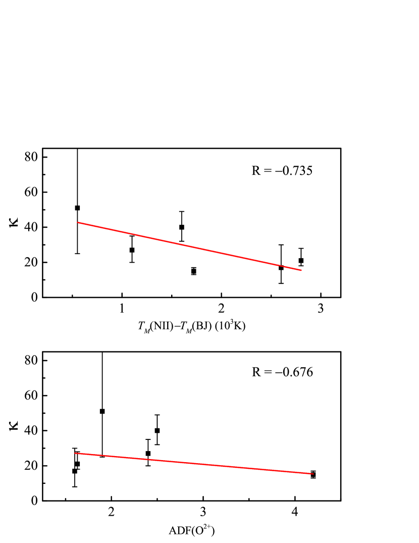
Figure 5: The $\kappa$ index vs $T_{M}$(N II)$-T_{M}$(BJ) (upper panel) and ADF(O²⁺) (lower panel). The solid lines represent linear fittings. The correlation coefficients are shown in the up-right corners.

We have investigated the feasibility of invoking the $\kappa$ EED to solve the “electron temperature and abundance discrepancy problem” encountered in PN studies. The electron temperature of the singly ionized C⁺ regions can be evaluated using the temperature inferred from the [N II] lines, $T_{M}$(N II). We have retrieved $T_{M}$(N II) from the literature (Table 1), which is generally found to be higher than $T_{M}({\rm BJ})$. Within the scenario of $\kappa$ EED, $T_{M}$(N II) strongly depends on the electronic high-energy tail, while the BJ depends mostly on the cold core of the distribution. It is interesting to note that the derived $T_{U}$ values consistently lie between $T_{M}$(N II) and $T_{M}({\rm BJ})$, suggesting that the temperature discrepancy can indeed be alleviated under the $\kappa$ EED hypothesis. The ratio between the O²⁺/H⁺ abundance derived from recombination lines and that derived from CELs, the so-called abundance discrepancy factor (ADF), is introduced to quantify the degree of abundance discrepancy. As listed in Table 1, the ADFs of our sample PNe range from 1.2 to 5.4. It is unfortunate that those nebulae with extremely large ADFs do not have C II UV lines detected. In Figure 5, we show that the $\kappa$ index negatively correlates with both $T_{M}$(N II)$-T_{M}$(BJ) and ADFs. This is compatible with the expectation that a larger departure from the MB EED should lead to larger temperature and abundance discrepancies. However, the correlation coefficients are only moderate, suggesting that the situation is not as simple as described here.

If the PN is homogeneous, that is, is presenting a constant EED, the $\kappa$ indices deduced from different diagnostic line ratios should have an identical value. For the purpose of comparison, Table 1 lists the $\kappa$ indices obtained by Zhang et al. (2016) using the [O III]$\lambda\lambda$4959,5007/$\lambda$4363 ratio and the H I BJ. The agreement is relatively marginal. In the framework of the $\kappa$-EED hypothesis, two effects can cause the disagreement between the $\kappa$ indices derived from the C II UV lines ($\kappa_{\rm CII}$) and those derived from [O III] CELs ($\kappa_{\rm OIII}$) as they go in opposite directions. If the variation of the EED with position was random, $\kappa_{\rm CII}$ would presumably be lower than $\kappa_{\rm OIII}$ since the excitation of the C II UV lines is more sensitive to the non-thermal tail of the EED as it preferentially takes place within the lower-$\kappa$ regions. The PN NGC 6153, which presents complex nebular structures, probably belongs to this category. On the other hand, deep integrated-field spectroscopy has revealed a globally increasing ADFs towards the center of PNe (García-Rojas et al., 2022). In this case, we would expect $\kappa_{\rm CII}>\kappa_{\rm OIII}$ since the [O III] and C II lines mainly trace the highly ionized inner region and the partially ionized outer layer, respectively. This might actually be the case for the high-excitation PN NGC 2440.

In any case, we can draw the firm conclusion that the $\kappa$ EED cannot be present in a homogeneous manner throughout the whole nebulae. On the other hand, current observations cannot rule out the development in PNe of local small-scale $\kappa$ EEDs. From the theoretical point of view, the main issue with the $\kappa$ EED hypothesis is the lack so far of a plausible mechanism for pumping the non-thermal electrons in PN environments. This might be the main reason for the fact that the $\kappa$ EED has been generally ignored in mainstream PN studies. However, we should be aware that the $\kappa$ distribution is a cutting edge research area in the field of solar plasma physics although its origin still remains unclear (e.g. Dudík & Dzifčáková, 2021; Dzifčáková et al., 2021). Furthermore, the other proposed solutions to the “electron temperature and abundance discrepancy problem” of PNe, such as temperature fluctuations or two-component models, are facing a similar challenge, namely, how to generate a sufficiently large $t^{2}$ or the hydrogen-deficient clumps? We therefore see no legitimate reason for the study of $\kappa$ distribution to be overlooked and undervalued by the PN research community. Recent studies reveal that high ADFs might be associated to the evolution of close binary central stars (Wesson et al., 2018) and, at this point, we may tentatively conjecture that a fast magnetosonic wave excited by the interaction with a strong stellar magnetic fields could instantly inject energetic electrons into the free-electron pool, thereby forming a $\kappa$ EED within the central regions of PNe.

We have built a toy two-EED model in an attempt to reproduce the observations, in which, besides a regular nebular component with a MB EED, we added a $\kappa$-EED component. In this scenario, the predicted C II line ratio is given by

$$r({\rm C~{}II})=\frac{\omega\epsilon_{\kappa}(2326;\kappa,T_{U})+(1-\omega)\epsilon_{M}(2326;T_{M})}{\omega\epsilon_{\kappa}(1335;\kappa,T_{U})+(1-\omega)\epsilon_{M}(1335;T_{M})}\,,$$ (6)

where $\omega$ is the volume filling factor of the $\kappa$-EED gas, and the emissivities of the $\kappa$- and MB-EED components, $\epsilon_{\kappa}(\lambda;\kappa,T_{U})$ and $\epsilon_{M}(\lambda;T_{M})$, are derived by solving level balance equations, as described in Section 3. For the sake of simplicity, we have assumed that the two components have identical density and temperature values, that is $T_{U}=T_{M}$ (where $T_{M}$ is derived from the BJ). Various $\kappa$ values have been found across the different solar plasmas, for instance, 3 in the outer solar corona, 4 in the outer heliosphere, 5 in the magnetotail, and 17 in the lower solar corona (Livadiotis, 2015). We have assumed that the $\kappa$-EED nebular component present values that are similar to those of solar plasmas, and calculate $r$(C II) for four preselected $\kappa$ values (3, 5, 10, and 20); the results are presented in Figure 6. It shows that with increasing filling factor ($\omega$) of the $\kappa$-EED component, the $r$(C II) versus $T_{M}$ relation changes from that of a uniform MB-EED ($\omega=0$) up to the case of a complete $\kappa$-EED ($\omega=1$). For a given $\omega$, there is a trend that, along with decreasing temperature, the $r$(C II) versus $T_{M}$ curves get progressively closer to the complete $\kappa$-EED case. This is because at such a low temperature, the MB-EED hardly excites the C II CELs unless non-thermal high-energy electrons exist, and thus in the low temperature case, the $r$(C II) ratio from Equ. 6 is essentially dominated by the $\kappa$-EED component.

The observed PN data are plotted in Figure 6. We can see that a very small amount of $\kappa$-EED gas with an extremely low $\kappa$ index is sufficient to explain the observations. For instance, we would require only 1–$5\%$ of the nebular gas to have $\kappa=3$ in order to reproduce the observed $r$(C II). If the non-thermal gas had a $\kappa$ value of 5 or 10, the required filling factor would need to increase up to $10\%$ or $50\%$. On the other hand, if one assumes $\kappa=20$, we could no longer reproduce the lowest $r$(C II) ratios. Alternatively, we could relax the assumption of a uniform temperature for the two components since the ejection of non-thermal electrons into the regular nebular gas is likely to cause $T_{U}$ to become $>T_{M}$. This would enhance the $\epsilon_{\kappa}$ value relative to $\epsilon_{M}$. As a result, the inferred $\omega$ would be further reduced (see Equ. 6). It therefore appears that the problem of the origin of $\kappa$-electrons pumping is not a very crucial issue.

6 Conclusion

The current work shows that the C II$\lambda\lambda$1335,2326 UV lines can serve as a useful tool to investigate the EED of PNe. The observed C II $\lambda 2326$/$\lambda$1335 intensity ratios are systematically lower than those expected with the MB-EED hypothesis. This would be satisfactorily explained if we assume the $\kappa$-EED hypothesis. We would suggest that the deviation from the MB-EED in PNe is lower than for AGNs. However, the $\kappa$-EED is unlikely to extend uniformly across the whole nebulae. Using a toy model of two-EED components, we have demonstrated that only a few percent of nebular gas in $\kappa$-EED is sufficient to reproduce the observations.

By no means can we state that the evidence of the existence of $\kappa$-EED in PNe is conclusive. Instead, we have shown that the generation of non-thermal electrons can definitely improve, rather than worsen, the agreement with the observations of C II UV lines as well as other emission lines. The same situation occurs with the Balmer continuum discontinuity, [O III], and O II observations (Zhang et al., 2014, 2016; Lin & Zhang, 2020), which supports the hypothesis that $\kappa$-EED on a small spatial scale is a promising solution to the “electron temperature and abundance discrepancy problem”. Further observational investigations of the influence of the $\kappa$ EED on other spectral features of PNe are eminently worth pursuing.

Figure 1: The IUE spectra of the PNe, which show the C II]$\lambda$2326 (left panel) and C II$\lambda$1335 (right panel) features. The smooth curves represent the Gaussian fits.

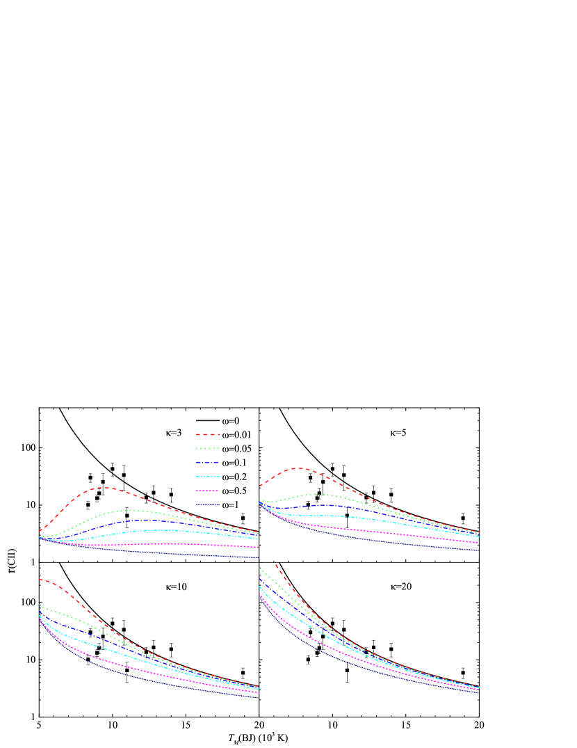
Figure 6: The relations between $r$(C II) and $T_{M}$(BJ) predicted by the two-EED model, which is composed of a regular MB-EED nebular component and a $\kappa$-EED component with a $\kappa$ index of 3, 5, 10, and 20 and various filling factors ($\omega$). The squares with error bars represent the observed values.

Table 1: The sample of PNe, with the flux and intensity measurements of the two C II UV features, and the diagnostic results. Note that the $F(\lambda)$ and $I(\lambda)$ are those of the blended features.

Objects	F($\lambda$) (10-13 $erg$ $cm^{-2}$ $s^{-1}$)		c(H$\beta$)a	I($\lambda$) (10-13 $erg$ $cm^{-2}$ $s^{-1}$)		$r$(C II)	$T_{M}$(N II)	$T_{M}$(BJ)	ADF	$\kappa$		$T_{U}$
	C II] $2326$	C II $1335$		C II] $2326$	C II $1335$		(K)	(K)		This	ref.l	(K)
NGC 2440	$1.64\pm 0.25$	$0.15\pm 0.03$	$0.42$	6.11 $\pm 0.91$	$0.59\pm 0.13$	$15.29\pm 4.02$	$10900$ b	$14000$ b	$5.4$ d	$\infty$	25	$14000$
NGC 2867	$51.11\pm 1.44$	$5.32\pm 0.81$	0.43	$196.20\pm 5.51$	$21.73\pm 3.01$	$13.22\pm 1.87$	$11750$ k	8950 k	1.63 k	$21_{-3}^{+7}$	15	9605
NGC 3132	$12.28\pm 0.59$	$0.53\pm 0.24$	0.16	$20.26\pm 0.97$	$0.89\pm 0.41$	$33.38\pm 15.29$	9350 c	10780 c	3.5 d	$\infty$	$\infty$	10780
NGC 3918	$8.45\pm 0.43$	$0.88\pm 0.17$	0.27	$19.66\pm 0.99$	$2.12\pm 0.41$	$13.58\pm 2.70$	10800 c	12300 c	1.8 d	>$100$	>$60$	12300
NGC 6543	$25.46\pm 3.66$	$3.61\pm 0.25$	0.12	$37.06\pm 5.33$	$5.35\pm 0.37$	$10.10\pm 1.62$	10060 h	8340 h	4.2 f	$15_{-2}^{+2}$	$\infty$	9267
NGC 6565	$8.53\pm 0.55$	$0.39\pm 0.06$	0.42	$31.74\pm 2.05$	$1.54\pm 0.24$	$30.18\pm 5.13$	10100 j	8500 j	1.69 j	$40_{-8}^{+9}$	24	8801
NGC 6572	$4.02\pm 0.20$	$0.86\pm 0.32$	0.34	$11.65\pm 0.58$	$2.6\pm 0.99$	$6.56\pm 2.51$	13600 e	11000 e	1.6 f	$17_{-9}^{+13}$	$\infty$	12065
NGC 6720	$17.99\pm 0.97$	$1.57\pm 0.31$	0.29	$44.58\pm 2.40$	$4.06\pm 0.80$	$16.10\pm 3.31$	10200 e	9100 e	2.4 f	$27_{-7}^{+8}$	32	9615
NGC 7027	$11.74\pm 0.84$	$0.87\pm 0.28$	1.24	$568.08\pm 40.41$	$50.47\pm 15.99$	$16.48\pm 5.35$	12900 g	12800 g	1.29 g	$\infty$	>$60$	12800
NGC 650	$3.29\pm 0.54$	$0.11\pm 0.02$	0.20	$6.15\pm 1.02$	$0.21\pm 0.04$	$42.89\pm 10.84$	10000:	10000:	*	$\infty$	$\infty$	10000:
IC 4406	$12.63\pm 3.74$	$0.70\pm 0.19$	0.28	$30.34\pm 8.99$	$1.74\pm 0.48$	$25.43\pm 10.32$	9900 c	9350 c	1.9 d	$51_{-26}^{+50}$	>$60$	9633
Hu 1-2	$7.03\pm 1.14$	$1.59\pm 0.21$	0.59	$44.52\pm 7.22$	$10.98\pm 1.45$	$5.94\pm 1.24$	13000 e	18900 e	1.6 f	$\infty$	$\infty$	18900

Table 2: The computed $r$(C II).

$T_{U}$(K)	$\kappa$
	2	3	5	10	20	30	50	$\infty$ (MB)
5000	1.088	2.63	10.39	50.47	128.69	226.10	919.40	3685.00
5200	1.083	2.54	9.38	42.58	106.30	189.60	687.70	2583.00
5400	1.079	2.47	8.55	36.41	89.20	160.19	525.50	1858.00
5600	1.074	2.40	7.85	31.54	75.84	136.39	409.39	1367.00
5800	1.069	2.33	7.26	27.62	65.27	116.90	324.60	1027.00
6000	1.065	2.27	6.75	24.44	56.80	101.00	261.39	786.90
6200	1.062	2.22	6.32	21.82	49.91	87.88	213.69	613.29
6400	1.059	2.17	5.95	19.65	44.25	76.97	176.89	485.50
6600	1.057	2.12	5.63	17.82	39.53	67.84	148.19	389.89
6800	1.054	2.08	5.34	16.29	35.57	60.15	125.50	317.10
7000	1.054	2.04	5.08	14.96	32.20	53.63	107.30	261.00
7200	1.052	2.00	4.86	13.81	29.31	48.07	92.58	217.19
7400	1.052	1.96	4.65	12.82	26.81	43.30	80.50	182.50
7600	1.051	1.93	4.47	11.96	24.64	39.18	70.52	154.80
7800	1.049	1.90	4.30	11.18	22.73	35.60	62.20	132.39
8000	1.049	1.87	4.15	10.51	21.06	32.49	55.21	114.09
8200	1.047	1.84	4.01	9.91	19.57	29.76	49.28	99.05
8400	1.047	1.81	3.88	9.37	18.25	27.36	44.23	86.57
8600	1.047	1.79	3.76	8.88	17.06	25.23	39.90	76.14
8800	1.046	1.77	3.65	8.44	16.00	23.35	36.16	67.36
9000	1.044	1.74	3.55	8.03	15.03	21.67	32.91	59.91
9200	1.042	1.72	3.45	7.67	14.16	20.17	30.07	53.56
9400	1.042	1.70	3.37	7.33	13.37	18.82	27.58	48.11
9600	1.041	1.69	3.28	7.03	12.65	17.60	25.38	43.41
9800	1.039	1.67	3.20	6.74	11.99	16.50	23.44	39.33
10000	1.037	1.65	3.13	6.48	11.38	15.50	21.71	35.77
10200	1.036	1.63	3.06	6.24	10.83	14.60	20.17	32.66
10400	1.034	1.62	2.99	6.01	10.31	13.77	18.79	29.92
10600	1.031	1.60	2.93	5.80	9.84	13.02	17.55	27.51
10800	1.029	1.59	2.87	5.61	9.40	12.33	16.43	25.36
11000	1.028	1.58	2.82	5.42	8.99	11.69	15.41	23.45
11200	1.026	1.56	2.76	5.25	8.61	11.11	14.49	21.75
11400	1.024	1.55	2.71	5.09	8.25	10.57	13.66	20.22
11600	1.021	1.54	2.66	4.94	7.92	10.07	12.89	18.85
11800	1.019	1.53	2.62	4.79	7.61	9.61	12.19	17.61
12000	1.016	1.51	2.57	4.66	7.32	9.18	11.55	16.49
12200	1.014	1.50	2.53	4.53	7.05	8.78	10.96	15.47
12400	1.011	1.49	2.49	4.41	6.80	8.41	10.42	14.55
12600	1.008	1.48	2.45	4.29	6.56	8.07	9.92	13.71
12800	1.006	1.47	2.41	4.18	6.33	7.74	9.46	12.94
13000	1.003	1.46	2.38	4.08	6.12	7.44	9.03	12.23
13200	1.001	1.45	2.34	3.98	5.92	7.16	8.63	11.58
13400	0.999	1.44	2.31	3.88	5.73	6.89	8.26	10.99
13600	0.997	1.43	2.28	3.79	5.55	6.64	7.91	10.44
13800	0.994	1.42	2.25	3.70	5.38	6.41	7.59	9.93
14000	0.992	1.41	2.22	3.62	5.22	6.18	7.29	9.46
14200	0.989	1.41	2.19	3.54	5.06	5.97	7.01	9.03
14400	0.987	1.40	2.16	3.47	4.92	5.78	6.74	8.63
14600	0.984	1.39	2.13	3.39	4.78	5.59	6.50	8.25
14800	0.982	1.38	2.11	3.32	4.64	5.41	6.26	7.90
15000	0.980	1.37	2.08	3.26	4.52	5.25	6.04	7.57
15200	0.977	1.37	2.06	3.19	4.40	5.09	5.84	7.27
15400	0.975	1.36	2.03	3.13	4.29	4.94	5.64	6.98
15600	0.973	1.35	2.01	3.07	4.18	4.80	5.46	6.72
15800	0.970	1.34	1.99	3.01	4.07	4.66	5.28	6.47
16000	0.968	1.33	1.96	2.96	3.97	4.53	5.12	6.23
16200	0.966	1.33	1.94	2.90	3.88	4.41	4.96	6.01
16400	0.964	1.32	1.92	2.85	3.79	4.29	4.82	5.80
16600	0.962	1.31	1.90	2.80	3.70	4.18	4.68	5.60
16800	0.960	1.30	1.88	2.75	3.61	4.07	4.54	5.41
17000	0.957	1.30	1.86	2.71	3.53	3.97	4.41	5.24
17200	0.955	1.29	1.84	2.66	3.45	3.87	4.29	5.07
17400	0.953	1.28	1.82	2.62	3.38	3.78	4.18	4.92
17600	0.951	1.28	1.80	2.58	3.31	3.69	4.07	4.77
17800	0.949	1.27	1.79	2.54	3.24	3.60	3.96	4.63
18000	0.947	1.26	1.77	2.50	3.17	3.52	3.86	4.49
18200	0.946	1.26	1.75	2.46	3.11	3.44	3.77	4.36
18400	0.944	1.25	1.74	2.42	3.05	3.36	3.67	4.24
18600	0.942	1.25	1.72	2.38	2.99	3.29	3.59	4.13
18800	0.940	1.24	1.70	2.35	2.93	3.22	3.50	4.01
19000	0.938	1.23	1.69	2.31	2.88	3.15	3.42	3.91
19200	0.936	1.23	1.67	2.28	2.82	3.09	3.35	3.81
19400	0.935	1.22	1.66	2.25	2.77	3.03	3.27	3.71
19600	0.933	1.22	1.64	2.22	2.72	2.97	3.20	3.62
19800	0.931	1.21	1.63	2.19	2.67	2.91	3.13	3.53
20000	0.929	1.20	1.62	2.16	2.63	2.85	3.07	3.45

Table 2: Continued.

References

- Bernard-Salas (2002) Bernard-Salas, J., Pottasch, S. R., Feibelman, W. A., & Wesselius, P. R. 2002, A&A, 387, 301
- Blum & Pradhan (1992) Blum, R. D., & Pradhan, A. K. 1992, ApJS, 80, 425
- Cahn et al. (1992) Cahn, J. H., Kaler, J. B., & Stanghellini, L. 1992, A&AS, 94, 399
- Danehkar (2021) Danehkar, A. 2021, ApJS, 257, 58
- Dopita et al. (2013) Dopita, M. A., Sutherland, R. S., Nicholls, D. C., Kewley, L. J., & Vogt, F. 2013, ApJS, 208, 10
- Draine & Kreisch (2018) Draine, B. T., & Kreisch, C. D. 2018, ApJ, 862, 30
- Dudík & Dzifčáková (2021) Dudík, J., & Dzifčáková, E. 2021, ASSL, 464, 53
- Dzifčáková et al. (2021) Dzifčáková, E., Dudík, J., Zemanová, A., et al. 2021, ApJS, 257, 62
- Ferland et al. (2016) Ferland, G. J., Henney, W. J., O’Dell, C. R., & Peimbert, M. 2016, RMxAA, 52, 261
- García-Rojas et al. (2017) García-Rojas, J., Corradi, R. L. M., Boffin, H. M. J., et al. 2017, in Liu, X., Stanghellini, L., Karakas, A., eds, Proc. IAU Symp. 323, Planetary Nebulae: Multi-Wavelength Probes of Stellar and Galactic Evolution. Cambridge Univ. Press, Cambridge, p. 65
- García-Rojas et al. (2022) García-Rojas, J., Morisset, C., Jones, D., et al. 2022, MNRAS, 510, 5444
- García-Rojas et al. (2009) García-Rojas, J., Peña, M., & Peimbert, A. 2009, A&A, 496, 139
- Hajduk et al. (2021) Hajduk, M., Haverkorn, M., Shimwell, H., et al. 2021, ApJ, 919, 121
- Hahn & Savin (2015) Hahn, M., & Savin, D. W. 2015, ApJ, 809, 178
- Howarth (1983) Howarth, I. D. 1983, MNRAS, 203, 301
- Humphrey & Binette (2014) Humphrey, A., & Binette, L. 2014, MNRAS, 442, 753
- Lin & Zhang (2020) Lin, B.-Z., & Zhang, Y. 2020, ApJ, 899, 33
- Liu et al. (2000) Liu, X.-W., Storey, P. J., Barlow, M. J., et al. 2000, MNRAS, 312, 585
- Liu et al. (2004a) Liu, Y., Liu, X.-W., Luo, S.-G., & Barlow, M. J. 2004, MNRAS, 353, 1231
- Liu et al. (2004b) Liu, Y., Liu, X.-W., Barlow, M. J., & Luo, S.-G. 2004, MNRAS, 353, 1251
- Livadiotis & McComas (2009) Livadiotis, G., & McComas, D. J. 2009, JGRA, 114, 11105
- Livadiotis & McComas (2011) Livadiotis, G., & McComas, D. J. 2011, ApJ, 741, 88
- Livadiotis (2015) Livadiotis, G. 2015, JGRA, 120, 1607
- Morais et al. (2021) Morais, S. G., Humphrey, A., Villar Martín, M., Binette, L., & Silva, M. 2021, MNRAS, 506, 1389
- Nicholls et al. (2012) Nicholls, D. C., Dopita, M. A., & Sutherland, R. S. 2012, ApJ, 752, 148
- Nicholls et al. (2013) Nicholls, D. C., Dopita, M. A., Sutherland, R. S., Kewley, L., & Palay, E. 2013, ApJS, 207, 21
- Nicolaou et al. (2018) Nicolaou, G., Livadiotis, G., Owen, C. J., Verscharen, D., & Wicks, R. T. 2018, ApJ, 864, 3
- Osterbrock & Ferland (2005) Osterbrock, D. E., & Ferland, G. J. 2005, Astrophysics of Gaseous Nebulae and Active Galactic Nuclei (2nd ed.; Sausalito, CA: University Science Books)
- Peimbert (1967) Peimbert, M. 1967, ApJ, 150, 825
- Pierrard & Lazar (2010) Pierrard, V., & Lazar, M. 2010, Sol. Phys., 265, 153
- Ruiz-Escobedo & Peña (2022) Ruiz-Escobedo, F., & Peña, M. 2022, MNRAS, 510, 5984
- Storey & Sochi (2013) Storey, P. J., & Sochi, T. 2013, MNRAS, 430, 599
- Storey & Sochi (2014) Storey, P. J., & Sochi, T. 2014, MNRAS, 440, 2581
- Torres-Peimbert et al. (1990) Torres-Peimbert, S., Peimbert, M., & Pena, M. 1990, A&A, 233, 540
- Tsamis et al. (2003) Tsamis, Y. G., Barlow, M. J., Liu, X.-W., Danziger, I. J., & Storey, P. J. 2003, MNRAS, 345, 186
- Tsamis et al. (2004) Tsamis, Y. G., Barlow, M. J., Liu, X.-W., Storey, P. J., & Danziger, I. J. 2004, MNRAS, 353, 953
- Vasyliunas (1968) Vasyliunas, V. M. 1968, J. Geophys. Res., 73, 2839
- Vernet et al. (2001) Vernet, J., Fosbury, R. A. E., Villar-Martín, M., et al. 2001, A&A, 366, 7
- Wang & Liu (2007) Wang, W., & Liu, X.-W. 2007, MNRAS, 381, 669
- Wesson et al. (2018) Wesson, R., Jones, D., García-Rojas, J., Boffin, H. M. J., & Corradi, R. L. M. 2018, MNRAS, 480, 4589
- Wesson & Liu (2004) Wesson, R., & Liu, X.-W. 2004, MNRAS, 351, 1026
- Wesson et al. (2005) Wesson, R., Liu, X.-W., & Barlow, M. J. 2005, MNRAS, 362, 424
- Zhang et al. (2005) Zhang, Y., Liu, X.-W., Luo, S.-G., Péquignot, D., & Barlow, M. J. 2005, A&A, 442, 249
- Zhang et al. (2004) Zhang, Y., Liu, X.-W., Wesson, R., et al. 2004, MNRAS, 351, 935
- Zhang et al. (2014) Zhang, Y., Liu, X.-W., & Zhang, B. 2014, ApJ, 780, 93
- Zhang et al. (2016) Zhang, Y., Zhang, B., & Liu, X.-W. 2016, ApJ, 817, 68