A simple micro-swimmer model inspired by the general equation for nonequilibrium reversible-irreversible coupling

Abstract

A simple mean-field micro-swimmer model is presented. The model is inspired by the nonequilibrium thermodynamics of multi-component fluids that undergo chemical reactions. These thermodynamics can be rigorously described in the context of the GENERIC (general equation for the nonequilibrium reversible-irreversible coupling) framework. More specifically this approach was recently applied to non-ideal polymer solutions (Indei and Schieber, J. Chem. Phys, 146, 184902, 2017). One of the species of the solution is an unreactive polymer chain represented by the bead-spring model. Using this detailed description as inspiration we then make several simplifying assumptions to obtain a mean-field model for a Janus micro-swimmer. The swimmer model considered here consists of a polymer dumbbell in a sea of reactants. One of the beads of the dumbbell is allowed to act as a catalyst for a chemical reaction between the reactants. We show that the mean-squared displacement, MSD, of the center of mass of this Janus dumbbell exhibits ballistic behavior at time scales at which the concentration of reactant is large. The time scales at which the ballistic behavior is observed in the MSD coincides with the time scales at which the cross-correlation between the swimmer’s orientation and the direction of its displacement exhibit a maximum. Since the swimmer model was inspired by the GENERIC framework it is possible to ensure that the entropy generation is always positive and therefore the second law of thermodynamics is obeyed.

This article may be downloaded for personal use only. Any other use requires prior permission of the author and AIP Publishing. This article appeared in A. Córdoba, J. D. Schieber and T. Indei, J. Chem. Phys. 152, 194902 (2020) and may be found at:
https://doi.org/10.1063/5.0003430.

1 Introduction

Swimming microorganisms, which include bacteria, algae, and spermatozoa, play a fundamental role in most biological processes. These swimmers are a special type of active particle, that continuously convert local energy into propulsive forces, thereby allowing them to move through their surrounding fluid medium. While the size, shape, and propulsion mechanism vary from one organism to the next, they all swim at small Reynolds numbers ^{1, 2, 3}. Microorganisms are able to overcome the thermal randomness of their surroundings by harvesting energy to navigate in viscous fluid environments. In a similar manner, synthetic colloidal microswimmers are capable of mimicking complex biolocomotion by means of simple self-propulsion mechanisms. Experimentally the speed of active particles can be controlled by e.g. self-generated chemical and thermal gradients, but an in-situ control of the swimming direction remains a challenge ². Artificial self-propelled micro- and nanoengines, or swimmers, have been increasingly attracting the interest of experimental and theoretical researchers. Synthetic microswimmers also work at low Reynolds number, where inertia does not sustain motion once the driving force stops, and often require complicated chemistry in both structural and dynamical terms ³.

Recent advances in microscopy techniques have allowed synthetic microswimmers to be studied experimentally ^{4, 2, 5, 6}. Janus particle swimmers made by coating fluorescent polymer beads with hemispheres of platinum have been fully characterized using video microscopy to reveal that they undergo propulsion in hydrogen peroxide fuel away from the catalytic platinum patch ⁴. The platinum coating shadows the fluorescence signal from half of each swimmer to allow the orientation to be observed directly and correlated quantitatively with the resulting swimming direction ⁴. Studies of self-propulsion of half-coated spherical colloids in critical binary mixtures have shown that the coupling of local body forces, induced by laser illumination, and the wetting properties of the colloid, can be used to finely tune both the colloid’s swimming speed and its directionality ². Among the few methods which have been proposed to create small-scale swimmers, those relying on self-phoretic mechanisms present an interesting design challenge in that chemical gradients are required to generate net propulsion ⁵. Asymmetries in geometry are sufficient to induce chemical gradients and swimming ⁵. Geometric asymmetries can be tuned to induce large locomotion speeds without the need of chemical patterning ⁵. The effect of the fuel concentration on the movement of self-assembled nanomotors based on polymersomes has also been studied. Positive control over the speed of these nanomotors and insights into the mechanism of propulsion have been reported ⁶.

Microswimmers have also been studied theoretically and through computer simulations ^{7, 8, 9, 10, 11, 15, 12, 13, 14, 16}. For instance, catalytic Janus particles which catalyze a chemical reaction inside the fluid and display self-propulsion have been studied extensively using simulations. It has been shown that the catalytic reaction produces an asymmetric, non-equilibrium distribution of reaction products around the colloid, which generates osmotic or other phoretic forces ^{13, 14, 15, 16, 3}. Analogous to the behavior of macroscopic motors the particle shape greatly matters and influences not only the random diffusion but also the efficiency of the propulsive motion ³. Coarser models of chemically propelled Janus swimmers have also been previously proposed ^{10, 1}. For example, the dynamical description of the motion of a stochastic microswimmer with constant speed and fluctuating orientation in the long time limit has been obtained by adiabatic elimination of the orientational variable ¹⁰. Starting with the corresponding full set of Langevin equations, the memory in the stochastic orientation is eliminated to obtain a stochastic equation for the position alone in the overdamped limit. An equivalent procedure based on the Fokker-Planck equation has been presented as well ¹⁰. Other simulations have used the squirmer model, which provides an ideal representation of swimmers as spheroidal particles that propel owing to a modified boundary condition at their surface. With this type of model the single-particle and many-particle dynamics of swimmers in bulk and confined systems have been studied using the smoothed profile method, which allows to efficiently solve the coupled particle-fluid problem ¹. Another line of work focuses on the collective behavior that emerges in moderately concentrated suspensions of swimmers ^{17, 18, 19, 20}. In those works individual swimmers are usually modeled using force dipoles. The hydrodynamic interactions between swimmers and/or confining walls are treated using Stokesian dynamics ²¹ or similar methods ²².

Moreover other theoretical studies have considered different types of swimming mechanisms ^{23, 1, 3, 7}. For example, swimmers comprising of two rigid spheres of different size which oscillate periodically along their axis of symmetry, have been shown to propel forward in viscoelastic fluids ⁷. The dynamics of a generalized three-sphere microswimmer in which the spheres are connected by two elastic springs have also been studied previously. The rest length of each spring was assumed to undergo a prescribed cyclic change ⁸. In the low-frequency region, the swimming velocity increases with frequency. Conversely, in the high-frequency region, the average velocity decreases with increasing frequency ⁸. Such behavior originates from the intrinsic spring relaxation dynamics of an elastic swimmer moving in a viscous fluid ⁸. A model swimmer consisting of two linked spheres, wherein one sphere is rigid and the other an incompressible neo-Hookean solid was also proposed ⁹. The two spheres are connected by a rod which changes its length periodically. Deformations of the body are non-reciprocal despite the reversible actuation and hence, the elastic two-sphere swimmer propels forward. These results indicate that even weak elastic deformations of a body can affect locomotion and may be exploited in designing artificial microswimmers ⁹. More recent work uses a model one-hinge artificial swimmer consisting of a bead spring model for two arms joined by a hinge with bending potential for the arms in order to make them semi-flexible ²³. These type of simulations have shown that when the swimmer has rigid arms, the center of mass of the swimmer is not able to propel itself. The flexibility in the arms causes the time reversal symmetry to break in the case of the one-hinged swimmer without the presence of a head ²³. The velocity of this type of swimmer has been studied using a range of parameters like flexibility, beating frequency and the amplitude of the beat ²³.

Thermodynamic analyses of microswimmers have also been attempted ^{11, 15, 12}. In one particular approach a potential thermodynamic efficiency was proposed by partially tethering the swimmer so that work is done externally and instantaneously ¹¹. This instantaneous definition has also been extended to encompass a full swimming stroke, and compute it for propulsion of a spherical body by a helical flagellum ¹¹. Scalar and vectorial steady-state fluctuation theorems and a thermodynamic uncertainty relation that link the fluctuating particle current to its entropy production at an effective temperature have been proposed ¹². Also analytical formulae from linear response theory have been extended to describe small swimmers, which interact with their environment on a finite length scale ¹⁵. Using irreversible, linear thermodynamics to formulate an energy balance the efficiency of transport for swimmers which are moving in random directions was shown to scale as the inverse of the macroscopic distance over which transport occurs ¹⁵.

Microswimmers operate far from equilibrium, therefore a complete and rigorous thermodynamic analysis of systems with microswimmers requires a thermodynamics framework capable of handling systems far from equilibrium. GENERIC is an equation to describe the time-evolution of the state variables not only near equilibrium but far from the equilibrium state ^{24, 25, 26}. GENERIC comprises reversible and irreversible contributions to the entire dynamics of the system. The reversible or mechanical contribution is driven by the gradient of the system energy with respect to the state variables, whereas the irreversible or dissipative dynamics is driven by the thermodynamic forces represented by the gradient of the entropy. Thus the two generators, the total energy and the total entropy of the system, drive the full dynamics of the system represented by the state variables. Another aspect of GENERIC is that it can be a useful tool to evaluate the thermodynamic consistency of coarse-grained models of complex soft materials ^{27, 28, 29}.

In the two-generator formalism of non-equilibrium thermodynamics ^{24, 25, 26} the time-evolution of a closed system is described by the equation,

$$\frac{d\bm{x}}{dt}=\bm{L}\cdot\frac{\delta E}{\delta\bm{x}}+\bm{M}\cdot\frac{\delta S}{\delta\bm{x}}.$$ (1)

Where $\bm{x}$ is a variable that represents the state of the system, $E$ is the total energy, and $S$ is the total entropy of the system. eq. (1) is called the GENERIC. The first term describes reversible dynamics. The reversible dynamics are driven by the gradient of the energy with respect to the state variable. The operator $\bm{L}$ is called the “Poisson matrix”. On the other hand, the second term represents the irreversible dynamics of the system. The irreversible dynamics are driven by the entropy gradient with respect to $\bm{x}$. The operator $\bm{M}$ is referred to as the “friction matrix”. There are several restrictions imposed on $\bm{L}$ and $\bm{M}$. First of all, these operators must satisfy the degeneracy conditions:

$$\bm{L}\cdot\frac{\delta S}{\delta\bm{x}}=\bm{0},\leavevmode\nobreak\ \leavevmode\nobreak\ \leavevmode\nobreak\ \leavevmode\nobreak\ \leavevmode\nobreak\ \bm{M}\cdot\frac{\delta E}{\delta\bm{x}}=\bm{0}.$$ (2)

Intuitively these requirements mean that the entropy gradient does not generate reversible dynamics whereas the energy gradient does not cause irreversible dynamics. In addition, $\bm{L}$ must be antisymmetric and satisfy the Jacobi identity, whereas $\bm{M}$ must be symmetric and positive semi-definite to guarantee a positive entropy generation rate or the second law of thermodynamics. The entropy generation rate density $\sigma$ can be obtained by applying the entropy gradient from the left of eq. (1) and by using the degeneracy requirement for the Poisson matrix, eq. (2), as

$$\sigma=\frac{\delta S}{\delta\bm{x}}\cdot\bm{M}\cdot\frac{\delta S}{\delta\bm{x}}.$$ (3)

In a recent paper Indei and Schieber ³⁰ reexamined the nonequilibrium thermodynamics of multi-component fluids that undergo chemical reactions and showed how to describe it in the context of the GENERIC framework. They applied this approach to polymer solutions. One of the species of the solution is the unreactive polymer chain represented by the bead-spring model. The polymer solution is neither dilute nor ideal. The solution entropy was constructed so that the contributions from mixing and chain conformation are fully separated.

GENERIC is an appropriate tool to check the thermodynamic consistency of a set of dynamical equations, even for active matter. The particular active system that is addressed in this paper are self-propelled microswimmers suspended in a Newtonian fluid ^{4, 2}. For example, Janus polystyrene spheres with a hemisphere covered with Pt. A catalytic reaction H_2O_2 -> 2H_2O + O_2 occurs at the Pt side of the particle and is the power source of the propulsion ⁴. Thus H_2O_2 molecules play the role of “fuel”. This reaction drives the swimmer along a particular direction inherent to the swimmer’s orientation. Though this active system is synthetic, this can be a good starting point for understanding more complex biological swimmers. Previous theoretical studies of diffusiophoretic microswimmers have used more detailed descriptions ^{13, 14, 15, 16, 3}. However, a coarse grained minimal level of description for diffusiophoretic microswimmers still remains to be identified. In this paper such a minimal level of description is proposed using GENERIC as a guide.

The remainder of this paper is organized as follows: Section 2 starts with a brief summary of the more general mass balance equations for a non-ideal solution of monodisperse polymer chains dissolved in a solvent that is undergoing chemical reactions ³⁰. The assumptions made to obtain the mean-field swimmer model considered here and the resulting mass balance equations are also given Section 2. To perform numerical simulations with the Janus swimmer model the mass balance equations are written as stochastic differential equations in the phase space, these are given at the end of Section 2. In Section 3 the entropy balance for the Janus swimmer model is derived. This balance allows the thermodynamic compliance of the Janus swimmer model to be readily checked. Finally, in Section 4, the predictions of the Janus swimmer model are presented and discussed.

2 Swimmer model

The swimmer model considered here is a bead-spring dumbbell with the position of bead $1$ given by $\bm{r}_{1}$ and the position of bead $2$ given by $\bm{r}_{2}$. The bond vector connecting the two beads is $\bm{Q}:=\bm{r}_{2}-\bm{r}_{1}$, and the center of gravity of the dumbbell is $\bm{r}_{c}:=\dfrac{\bm{r}_{1}+\bm{r}_{2}}{2}$. The inertia of the beads is neglected and over-damped dynamics are considered for the equations of motion of the dumbbell. The dumbbell is dissolved in a solvent formed by species $\alpha$ and $\beta$. Bead $1$ of the dumbbell acts as a catalyst for the irreversible chemical reaction $|\nu_{\alpha}|\alpha\longrightarrow|\nu_{\beta}|\beta$, where $\nu_{\alpha}$ and $\nu_{\beta}$ are stoichiometric coefficients.

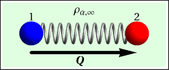
Figure 1: Sketch of the simple swimmer model considered in this work. The swimmer model considered here is a bead-spring dumbbell with the position of bead $1$ given by $\bm{r}_{1}$ and the position of bead $2$ given by $\bm{r}_{2}$, the following definitions are also used throughout the text, $\bm{Q}:=\bm{r}_{2}-\bm{r}_{1}$ and $\bm{r}_{c}:=\dfrac{\bm{r}_{1}+\bm{r}_{2}}{2}$. The radius of both beads is $R$. Bead $1$ acts as a catalyst for the irreversible chemical reaction $|\nu_{\alpha}|\alpha\longrightarrow|\nu_{\beta}|\beta$. The swimmer is in a sea (or bath) of reactants and the concentration of reactant, is equal to $\rho_{\alpha,\infty}$.

Before giving the simplified equations for the mean-field swimmer model that will be considered here, the more general mass balance equations for a non-ideal solution of monodisperse polymer chains ³⁰ is briefly recapitulated. In general, an adequate set of state variables to describe the system discussed above is:

$$\bm{x}(\bm{r},t)=\left\{\rho_{\alpha}(\bm{r}),\rho_{\beta}(\bm{r}),\rho_{c}(\bm{r},\bm{Q}),\bm{u}(\bm{r}),\epsilon(\bm{r})\right\}$$ (4)

where $\bm{r}$ is a position in space, $\rho_{\alpha}(\bm{r})$ and $\rho_{\beta}(\bm{r})$ are the mass densities of the $\alpha$ and $\beta$ species, respectively; $\rho_{c}(\bm{r},\bm{Q})$ is the mass density of dumbbells; $\bm{u}=\bm{v}\left(\rho_{c}+\rho_{\alpha}+\rho_{\beta}\right)$ is the momentum density with $\bm{v}$ the velocity; and $\epsilon(\bm{r})$ is the internal energy density. Note that $\rho_{c}(\bm{r},\bm{Q})$ may also be interpreted as the probability density of finding a dumbbell with its center of mass at position $\bm{r}$ and with end-to-end vector $\bm{Q}$. Is this latter interpretation that will be used in the remainder of this article.

The mass balance equation for the bead-spring Janus dumbbells is,

$$\frac{\partial\rho_{c}(\bm{r},\bm{Q})}{\partial t}= -\frac{\partial}{\partial\bm{r}}\cdot\left[\rho_{c}(\bm{r},\bm{Q})\bm{v}(\bm{r})+\bm{j}_{c}^{\rm diff}(\bm{r},\bm{Q})\right]$$ (5)

$$-\frac{\partial}{\partial\bm{Q}}\cdot\left[\rho_{c}(\bm{r},\bm{Q})\nabla\bm{v}(\bm{r})^{\dagger}\cdot\bm{Q}+\bm{j}^{\rm conf}(\bm{r},\bm{Q})\right].$$

Where $\rho_{c}(\bm{r},\bm{Q})$ is the mass density of dumbbells. The diffusional flux of the dumbbells is given by,

$$\bm{j}^{\rm diff}_{c}(\bm{r},\bm{Q})= -D^{\prime}_{c\alpha}(\bm{r},\bm{Q})\frac{\partial}{\partial\bm{r}}\frac{\mu_{\alpha}(\bm{r})}{T(\bm{r})}-D^{\prime}_{c\beta}(\bm{r},\bm{Q})\frac{\partial}{\partial\bm{r}}\frac{\mu_{\beta}(\bm{r})}{T(\bm{r})}$$ (6)

$$-D^{\prime}_{cc}(\bm{r},\bm{Q})\frac{\partial}{\partial\bm{r}}\frac{\mu_{c}(\bm{r},\bm{Q})}{T(\bm{r})}.$$

Where $\mu_{\alpha}(\bm{r})$ and$\mu_{\beta}(\bm{r})$ are the chemical potentials of species $\alpha$ and $\beta$ respectively. $D^{\prime}_{c\alpha}$, $D^{\prime}_{c\beta}$ and $D^{\prime}_{cc}$ are diffusion coefficients and $T$ is the temperature. The configurational flux of the Janus dumbbells is given by,

$$\bm{j}^{\rm conf}(\bm{r},\bm{Q})= -4D^{\prime}_{cc}(\bm{r},\bm{Q})\frac{\partial}{\partial\bm{Q}}\left[\frac{\mu_{c}(\bm{r},\bm{Q})}{T(\bm{r})}+\frac{\phi^{(E)}(\bm{Q})}{m_{c}T(\bm{r})}\right].$$ (7)

Where $\phi^{(E)}(\bm{Q})$ is the enthalpic part of the free energy of the spring that connects the two beads and $\mu_{c}(\bm{r},\bm{Q})$ is the chemical potential of a dumbbell per mass,

$$m_{c}\mu_{c}(\bm{r},\bm{Q})=m_{c}\mu_{c}(\bm{r})+\phi^{(S)}(\bm{r},\bm{Q})+k_{\rm B}T(\bm{r})\log\frac{\rho_{c}(\bm{r},\bm{Q})}{z\rho_{c}(\bm{r})}.$$ (8)

Here $m_{c}$ is the mass of one dumbbell, $\phi^{S}(\bm{r},\bm{Q})$ is the entropic part of the free energy of the spring connecting the two beads, $\rho_{c}(\bm{r}):=\int\rho_{c}(\bm{r},\bm{Q})d\bm{Q}$, and $z$ is a normalization constant. Note that eqs. (6) and (7) are identical to the balance equations for a multi-component non-ideal polymer solution given in previous work ³⁰.

The mass balance equations for species $\alpha$ ad $\beta$ are,

$$\frac{\partial\rho_{\alpha}(\bm{r},\bm{Q})}{\partial t}=-\frac{\partial}{\partial\bm{r}}\cdot\left[\rho_{\alpha}(\bm{r})\bm{v}(\bm{r})+\bm{j}_{\alpha}^{\rm diff}(\bm{r},\bm{Q})\right]+m_{\alpha}\nu_{\alpha}J(\bm{r}),$$ (9a)

$$\frac{\partial\rho_{\beta}(\bm{r},\bm{Q})}{\partial t}=-\frac{\partial}{\partial\bm{r}}\cdot\left[\rho_{\beta}(\bm{r})\bm{v}(\bm{r})+\bm{j}_{\beta}^{\rm diff}(\bm{r},\bm{Q})\right]+m_{\beta}\nu_{\beta}J(\bm{r}).$$ (9b)

Where,

$$\bm{j}_{\alpha}^{\rm diff}= -D^{\prime}_{\alpha\alpha}(\bm{r})\frac{\partial}{\partial\bm{r}}\frac{\mu_{\alpha}(\bm{r})}{T(\bm{r})}-D^{\prime}_{\alpha\beta}(\bm{r})\frac{\partial}{\partial\bm{r}}\frac{\mu_{\beta}(\bm{r})}{T(\bm{r})}-D^{\prime}_{\alpha c}(\bm{r},\bm{Q})\frac{\partial}{\partial\bm{r}}\frac{\mu_{c}(\bm{r})}{T(\bm{r})},$$ (10a)

$$\bm{j}_{\beta}^{\rm diff}= -D^{\prime}_{\beta\beta}(\bm{r})\frac{\partial}{\partial\bm{r}}\frac{\mu_{\beta}(\bm{r})}{T(\bm{r})}-D^{\prime}_{\beta\alpha}(\bm{r})\frac{\partial}{\partial\bm{r}}\frac{\mu_{\alpha}(\bm{r})}{T(\bm{r})}-D^{\prime}_{\beta c}(\bm{r},\bm{Q})\frac{\partial}{\partial\bm{r}}\frac{\mu_{c}(\bm{r})}{T(\bm{r})}.$$ (10b)

$J(\bm{r})$ is the reaction rate and $\mu_{c}(\bm{r}):=\int\mu_{c}(\bm{r},\bm{Q})d\bm{Q}$. Here also the mass balance equations are the same as the ones previously derived for a multi-component non-ideal polymer solution ³⁰. Moreover, since the total mass flux has to be conserved the diffusion coefficients $D^{\prime}_{c\alpha}$, $D^{\prime}_{c\beta}$ are coupled to $D^{\prime}_{cc}$ through ³⁰,

$$D^{\prime}_{cc}(\bm{r},\bm{Q})+D^{\prime}_{c\alpha}(\bm{r},\bm{Q})+D^{\prime}_{c\beta}(\bm{r},\bm{Q})=0.$$ (11)

Additionally to the mass balance equations for the solvent species, eq. (9), and the mass balance for the dumbbell, eq. (5), balance equations for the remaining state variables, the momentum density and the total energy density, have also been previously obtained using GENERIC for the non-ideal solution of monodisperse polymer chains ³⁰. However they will not be used in this manuscript and therefore they are not rewritten here.

Note that in general eqs. (9) and (5) represent a system of coupled equations for $\rho_{\alpha}(\bm{r})$, $\rho_{\beta}(\bm{r})$ and $\rho_{c}(\bm{r},\bm{Q})$. In principle, after specifying a reaction rate $J(\bm{r})$ this system of equations together with the balances for $\bm{u}(\bm{r})$ and $\epsilon(\bm{r})$ can be solved numerically for some given boundary conditions. In this work a different approach is taken, here the purpose is to obtain a mean-field model of a single Janus microswimmer in which the thermodynamic compliance can be readily checked. The swimmer is in a sea (or bath) of reactants and the concentration of reactant in the bath is equal to $\rho_{\alpha,\infty}$. Note that $\rho_{\alpha,\infty}$ will be allowed to change with time, but it will not be a field variable. Fig. 1 shows a sketch of the Janus swimmer model considered here. The level of description (set of state variables) of the model then reduces to,

$$\bm{x}(\bm{r}_{c},\bm{Q})=\left\{\rho_{\alpha,\infty},\rho_{c}(\bm{r}_{c},\bm{Q}),\epsilon(\bm{r}_{c})\right\}.$$ (12)

Moreover it will be assumed that very near bead $1$ of the dumbbell, i.e. the catalytic bead, the concentration of species $\alpha$ is always very small and will be approximated to be always zero. At a distance $\ell_{0}$ away, near bead $2$ of the dumbbell, the concentration of of species $\alpha$ will be assumed to always be equal to $\rho_{\alpha,\infty}$. Therefore the concentration gradient for $\alpha$ will be in the direction of $\bm{Q}$ and can be approximated as,

$$\dfrac{\partial\rho_{\alpha}(\bm{r}_{c})}{\partial\bm{r}_{c}}\approx\dfrac{\bm{Q}}{Q}\frac{\rho_{\alpha,\infty}}{\ell_{0}}\frac{\rho_{c}(\bm{r}_{c},\bm{Q})}{\rho_{c}}.$$ (13)

Where $Q:=|\bm{Q}|$ is the magnitude of $\bm{Q}$. Since a single swimmer in a mean-field is being considered then from now on $\dfrac{\rho_{c}(\bm{r}_{c},\bm{Q})}{\rho_{c}}$ is interpreted as the probability density of finding a dumbbell with its center of mass at position $\bm{r}_{c}$ and end-to-end vector $\bm{Q}$. With $\rho_{c}:=\dfrac{\int\int\rho_{c}(\bm{r}_{c},\bm{Q})d\bm{Q}d\bm{r}_{c}}{V}=\dfrac{m_{c}}{V}$ being the normalization factor for the probability density. And $V$ is the total volume of the container where the dumbbell is swimming. Similarly, across the swimmer there will also be a concentration gradient for species $\beta$ that can be approximated as,

$$\dfrac{\partial\rho_{\beta}(\bm{r}_{c})}{\partial\bm{r}_{c}} \approx-\dfrac{\bm{Q}}{Q}\frac{1}{\ell_{0}}\left(\rho_{\beta,\infty}+\frac{|\nu_{\beta}|}{|\nu_{\alpha}|}\frac{m_{\beta}}{m_{\alpha}}\rho_{\alpha,\infty}-\rho_{\beta,\infty}\right)\frac{\rho_{c}(\bm{r}_{c},\bm{Q})}{\rho_{c}}$$ (14)

$$=-\dfrac{\bm{Q}}{Q}\frac{\rho_{\alpha,\infty}}{\ell_{0}}\frac{\rho_{c}(\bm{r}_{c},\bm{Q})}{\rho_{c}}.$$

Where $\rho_{\beta,\infty}$ is the concentration of $\beta$ near bead $2$ of the dumbbell, and $\rho_{\beta,\infty}+\dfrac{|\nu_{\beta}|}{|\nu_{\alpha}|}\dfrac{m_{\beta}}{m_{\alpha}}\rho_{\alpha,\infty}$ is the concentration of $\beta$ near the catalytic bead of the dumbbell, i.e. bead $1$; $m_{\alpha}$ and $m_{\beta}$ are the molecular weights of $\alpha$ and $\beta$ respectively. In the second line of eq. (14) the fact that $\dfrac{|\nu_{\beta}|}{|\nu_{\alpha}|}\dfrac{m_{\beta}}{m_{\alpha}}=1$ due to mass conservation has been used.

With the approximations for the concentration gradients of $\alpha$ and $\beta$ near the swimmer, eqs. (13) and (14), assuming constant temperature and using the chain rule for the gradients of the chemical potentials, e.g. $\frac{\partial\mu_{\alpha}(\bm{r})}{\partial\bm{r}}=\bigg{\{}\frac{\partial\rho_{\alpha}(\bm{r})}{\partial\bm{r}}\left[\frac{\partial\mu_{\alpha}(\bm{r})}{\partial\rho_{\alpha}(\bm{r})}\right]_{T,p,\rho_{\beta},\rho_{c}}+\frac{\partial\rho_{\beta}(\bm{r})}{\partial\bm{r}}\left[\frac{\partial\mu_{\alpha}(\bm{r})}{\partial\rho_{\beta}(\bm{r})}\right]_{T,p,\rho_{\alpha},\rho_{c}}+\frac{\partial\rho_{c}(\bm{r},\bm{Q})}{\partial\bm{r}}\left[\frac{\partial\mu_{\alpha}(\bm{r})}{\partial\rho_{c}(\bm{r},\bm{Q})}\right]_{T,p,\rho_{\alpha},\rho_{\beta}}\bigg{\}}$ the diffusional flux of the Janus dumbbell, eq. (6), can be written as,

$$\bm{j}^{\rm diff}_{c}(\bm{r}_{c},\bm{Q})= -\bigg{[}D^{\prime}_{c\alpha}(\bm{r}_{c},\bm{Q})\gamma^{\prime}_{\alpha}(\bm{r}_{c},\bm{Q})+D^{\prime}_{c\beta}(\bm{r}_{c},\bm{Q})\gamma^{\prime}_{\beta}(\bm{r}_{c},\bm{Q})\bigg{]}\frac{\bm{Q}}{Q}\frac{\rho_{\alpha,\infty}}{\ell_{0}}\frac{\rho_{c}(\bm{r}_{c},\bm{Q})}{\rho_{c}}$$ (15)

$$-\bigg{[}D^{\prime}_{c\alpha}(\bm{r}_{c},\bm{Q})\gamma^{\prime}_{c\alpha}(\bm{r}_{c},\bm{Q})+D^{\prime}_{c\beta}(\bm{r}_{c},\bm{Q})\gamma^{\prime}_{c\beta}(\bm{r}_{c},\bm{Q})\bigg{]}\frac{\partial\rho_{c}(\bm{r}_{c},\bm{Q})}{\partial\bm{r}_{c}}.$$

Where $\gamma^{\prime}_{\alpha}(\bm{r}_{c},\bm{Q})$, $\gamma^{\prime}_{\beta}(\bm{r}_{c},\bm{Q})$, $\gamma^{\prime}_{c\alpha}(\bm{r}_{c},\bm{Q})$ and $\gamma^{\prime}_{c\beta}(\bm{r}_{c},\bm{Q})$ are thermodynamic derivatives of the chemical potentials with respect to the densities. The definitions for $\gamma^{\prime}_{\alpha}(\bm{r}_{c},\bm{Q})$, $\gamma^{\prime}_{\beta}(\bm{r}_{c},\bm{Q})$, $\gamma^{\prime}_{c\alpha}(\bm{r}_{c},\bm{Q})$ and $\gamma^{\prime}_{c\beta}(\bm{r}_{c},\bm{Q})$ are given in Section S1 of the Supplementary Information. Furthermore, assuming that the spring connecting the two beads is purely entropic the configurational flux of the dumbbell, eq. (7), can be written as,

$$\bm{j}^{\rm conf}(\bm{r}_{c},\bm{Q})= -4\gamma^{\prime}_{cc}(\bm{r}_{c},\bm{Q})\bigg{[}D^{\prime}_{c\alpha}(\bm{r}_{c},\bm{Q})+D^{\prime}_{c\beta}(\bm{r}_{c},\bm{Q})\bigg{]}\left[\frac{\partial\rho_{c}(\bm{r}_{c},\bm{Q})}{\partial\bm{Q}}+\frac{m_{c}}{k_{\rm B}T}\frac{\partial\phi^{(S)}(\bm{Q})}{\partial\bm{Q}}\right].$$ (16)

Where it has been assumed that the spring connecting the two beads is purely entropic and therefore $\phi^{(S)}(\bm{Q})$ is all the free energy of the spring. Also, in what follows $D^{\prime}_{c\alpha}$, $D^{\prime}_{c\beta}$, $\gamma^{\prime}_{\alpha}$, $\gamma^{\prime}_{\beta}$, $\gamma^{\prime}_{c\alpha}$, $\gamma^{\prime}_{c\beta}$ and $\gamma^{\prime}_{cc}$ will be assumed to be independent of $\bm{r}_{c}$ and $\bm{Q}$. Note that since near the swimmer the mass fluxes of the two solvent species are equal in magnitude but opposite in direction. Then, the terms in the mass balance equation for the dumbbell, eq. (5), involving the velocity, $\bm{v}(\bm{r}_{c})$, vanish i.e., $\rho_{c}(\bm{r}_{c},\bm{Q})\bm{v}(\bm{r}_{c})=0$ and $\rho_{c}(\bm{r}_{c},\bm{Q})\nabla\bm{v}(\bm{r}_{c})^{\dagger}=0$.

The approximations for the gradients of the reactants near the swimmer, eq. (13) and eq. (14), effectively decouple the mass balance equation for the dumbbell from the mass balance equations for the reactants. However, for the level of description of the mean-field swimmer model one can write an evolution equation for the concentration of reactant in the bath,

$$\frac{d\rho_{\alpha,\infty}(t)}{dt}=-J(t).$$ (17)

Where the net reaction rate $J(t)$ now includes both the mass transport of reactants from the bath to the dumbbell and also the reaction rate once the reactants reach the catalyst-coated bead of the Janus dumbbell. Therefore the net reaction rate, $J(t)$, can be written as,

$$J(t)=\left(\frac{4\pi R^{2}}{V}\right)\frac{1}{1/J_{r}(t)+1/J_{m}(t)}.$$ (18)

Where $J_{r}(t)$ is the rate of reaction at the surface of the catalyst coated bead and $J_{m}(t)$ is the rate associated with the mass transport of reactants from the bulk to the swimmer. $R$ is the radius of the catalyst-coated bead and $V$ is the volume of the container where the Janus dumbbell is swimming. The specific form for the reaction rate used in eq. (18) is based on the solution to a problem with similar physics. That is, binary diffusion through a boundary layer and reaction at a surface ³¹. See Section S3 of the Supplementary Information for more details on this regard. In general, for the reaction rate, $J_{r}(t)$, the following form can be employed,

$$J_{r}(t)=|\nu_{\alpha}|k^{\prime\prime}\rho_{\alpha,\infty}(t)^{|\nu_{\alpha}|}.$$ (19)

Where $k^{\prime\prime}$ is a rate constant for the reaction at the surface of the catalyst-coated bead of the Janus dumbbell. Here, we will consider only first order reactions, that is $\nu_{\alpha}=-1$. Assuming $D^{\prime}_{\alpha\alpha}$ and $\gamma_{\alpha\alpha}$ independent of $\bm{r}$, and using the approximation for the gradients introduced in eqs. (13) and (14) the rate associated with mass transport of reactants from the bulk to the swimmer may be written as,

$$J_{m}(t)=D^{\prime}_{\alpha\alpha}\gamma_{\alpha\alpha\beta}\frac{\rho_{\alpha,\infty}(t)}{\ell_{0}}.$$ (20)

Therefore the net reaction rate can be written as,

$$J(t)=\left(\frac{4\pi R^{2}}{V}\right)\frac{k^{\prime\prime}\gamma_{\alpha\alpha\beta}D^{\prime}_{\alpha\alpha}\rho_{\alpha,\infty}(t)}{\gamma_{\alpha\alpha\beta}D^{\prime}_{\alpha\alpha}+\ell_{0}k^{\prime\prime}}.$$ (21)

Is also useful to write the net reaction rate, eq. (21) in dimensionless form,

$$\hat{J}(t)=X_{S}\left(\frac{X_{\rho}(t)X_{r}}{X_{r}\hat{\ell}_{0}+1}\right).$$ (22)

Where $X_{r}:=\dfrac{k^{\prime\prime}}{D^{\prime}_{\alpha\alpha}\gamma_{\alpha\alpha\beta}}\sqrt{\dfrac{k_{\rm B}T}{k_{b}}}$ and $X_{S}:=\dfrac{4\pi R^{2}}{V}\sqrt{\dfrac{k_{\rm B}T}{k_{b}}}$. Note that $X_{r}$ is a ratio between two time scales. The time scale for the mass transfer of reactant from the bath to the dumbbell, in the numerator, and in the denominator the time scale of the reaction at the surface of the catalytic bead. Therefore values of $X_{r}>1$ correspond to an overall reaction rate that is more limited by the mass transport of reactants while values of $X_{r}<1$ correspond to a reaction rate that is more limited by the chemical kinetics.

Using the simplified fluxes, eqs. (15) and (16), it is now possible to write the mass balance for the swimmer, eq. (5), in the phase space as a set of stochastic differential equations (SDEs) for $\bm{Q}$ and $\bm{r}_{c}$ ^{32, 33},

$$d\bm{Q}= \frac{2\gamma^{\prime}_{cc}\left(D^{\prime}_{c\alpha}+D^{\prime}_{c\beta}\right)}{k_{\rm B}T}\frac{\partial\phi^{(S)}}{\partial\bm{Q}}dt+\sqrt{4\gamma^{\prime}_{cc}\left(D^{\prime}_{c\alpha}+D^{\prime}_{c\beta}\right)}d\bm{W}_{1}(t),$$ (23)

$$d\bm{r}_{c}= \left[\frac{\rho_{\alpha,\infty}(t)}{\ell_{0}\rho_{c}}\left(D^{\prime}_{c\alpha}\gamma^{\prime}_{\alpha}+D^{\prime}_{c\beta}\gamma^{\prime}_{\beta}\right)\frac{\bm{Q}}{Q}\right]dt+\sqrt{D^{\prime}_{c\alpha}\gamma^{\prime}_{c\alpha}+D^{\prime}_{c\beta}\gamma^{\prime}_{c\beta}}d\bm{W}_{2}(t).$$

Where $d\bm{W}_{1}$ and $d\bm{W}_{2}$ are vectors of Wiener increments with statistics, $\left\langle{d\bm{W}}_{i}(t)\right\rangle_{\rm eq}=\bm{0}$ and $\left\langle{d\bm{W}}_{i}(t){d\bm{W}}_{j}(t^{\prime})\right\rangle_{\rm eq}=\bm{\delta}\delta(t-t^{\prime})\delta_{ij}dtdt^{\prime}$. In what follows it will be assumed that $\phi^{(S)}=-\dfrac{k_{b}(Q-\ell_{0})^{2}}{2}$, with $k_{b}$ the entropic spring constant. Note that in eq. (23) the first term on the right hand side of the equation for the center of mass of the dumbbell can be interpreted as the swimming velocity. The swimming velocity is directly proportional to the concentration of reactant in the bath, $\rho_{\alpha,\infty}$, and inversely proportional to the rest length of the dumbbell, $\ell_{0}$. Shorter dumbbells produce larger concentrations gradients around them, which in turn produces a larger swimming velocity. To perform Brownian dynamics (BD) simulations of the swimmer model eq. (23) is first made dimensionless. The dimensionless form of eq. (23) is given in the Supplementary Information, eq. (S17). In what follows dimensionless variables are written with a hat.

3 Entropy Balance

In the GENERIC framework the entropy generation rate density of a model can be calculated using eq. (3). In general, the entropy generation rate should always be positive to guarantee that the model satisfies the second law of thermodynamics. Assuming constant temperature and using the chain rule for the chemical potential gradients it can be shown, see Sec. S2 in the Supplementary Information, that the entropy generation rate density for the dumbbell in a bath of reactants reduces to,

$$\sigma= \frac{\mu_{\alpha,\infty}(t)}{T}J(t)+\frac{A_{c}}{VT}\int\int\left[\frac{\rho_{\alpha,\infty}}{\ell_{0}}\frac{\rho_{c}(\bm{r}_{c},\bm{Q})}{\rho_{c}}\right]^{2}d\bm{Q}d\bm{r}_{c}$$ (24)

$$+ \frac{C_{c}}{VT}\int\int\left[\dfrac{\partial\rho_{c}(\bm{r}_{c},\bm{Q})}{\partial\bm{r}_{c}}\cdot\dfrac{\partial\rho_{c}(\bm{r}_{c},\bm{Q})}{\partial\bm{r}_{c}}\right]d\bm{Q}d\bm{r}_{c}$$

$$+ \frac{4\gamma^{2}_{cc}(D^{\prime}_{c\alpha}+D^{\prime}_{c\beta})}{VT}\int\int\left[\frac{\partial\rho_{c}(\bm{r}_{c},\bm{Q})}{\partial\bm{Q}}\cdot\frac{\partial\rho_{c}(\bm{r}_{c},\bm{Q})}{\partial\bm{Q}}\right]d\bm{Q}d\bm{r}_{c}.$$

Where $\mu_{\alpha,\infty}$ is the chemical potential of reactant in the bath. Note that the first term in eq. (24) includes the entropy generation due to the diffusion of reactant from the bath to the swimmer and also includes the entropy generation due to the chemical reaction at the surface of the catalytic bead. If $\mu_{\alpha,\infty}$ is assumed to depend linearly on $\rho_{\alpha,\infty}$ then this term is always positive for the reaction flux, eq. (21), used here. The term in the last line of eq. (24), is quadratic in $\dfrac{\partial\rho_{c}(\bm{r}_{c},\bm{Q})}{\partial\bm{Q}}$ and therefore always positive as long as $D^{\prime}_{c\alpha}$ and $D^{\prime}_{c\beta}$ are positive. Also the following parameters were introduced,

$$A_{c}:= D^{\prime}_{c\alpha}\gamma_{c\alpha\beta}\left[\gamma_{\alpha\alpha\beta}-\gamma_{c\alpha\beta}\right]+D^{\prime}_{c\beta}\gamma_{c\alpha\beta}\left[\gamma_{\beta\alpha\beta}-\gamma_{c\alpha\beta}\right]$$ (25)

$$C_{c}:= D^{\prime}_{c\alpha}\gamma_{cc}\left[\gamma_{\alpha c}-\gamma_{cc}\right]+D^{\prime}_{c\beta}\gamma_{cc}\left[\gamma_{\beta c}-\gamma_{cc}\right].$$

The definitions for the thermodynamic derivatives, $\gamma_{c\alpha\beta}$, $\gamma_{\alpha\alpha\beta}$, $\gamma_{\beta\alpha\beta}$, $\gamma_{cc}$, $\gamma_{\alpha c}$ and $\gamma_{\beta c}$, are given in eq. (S2) of the Supplementary Information. The remaining terms on the right side of eq. (24) always stay positive as long as $A_{c}>0$ and $C_{c}>0$. Since $D^{\prime}_{c\alpha}$ and $D^{\prime}_{c\beta}$ are positive then the restrictions on $A_{c}$ and $C_{c}$ translate into restrictions on the $\gamma$’s. Is illustrative to assume $\gamma_{\beta\alpha\beta}=\gamma_{\alpha\alpha\beta}$ and $\gamma_{\beta c}=\gamma_{\alpha c}$ in which case those restrictions simplify to,

$$\gamma_{\alpha\alpha\beta}>\gamma_{c\alpha\beta},\leavevmode\nobreak\ \leavevmode\nobreak\ \leavevmode\nobreak\ \leavevmode\nobreak\ \gamma_{\alpha c}>\gamma_{cc}.$$ (26)

Or in terms of $\gamma^{\prime}_{\alpha}$, $\gamma^{\prime}_{\beta}$, $\gamma^{\prime}_{c\alpha}$, and $\gamma^{\prime}_{c\beta}$ the restrictions are,

$$\gamma^{\prime}_{\alpha}>0,\leavevmode\nobreak\ \leavevmode\nobreak\ \leavevmode\nobreak\ \gamma^{\prime}_{c\alpha}>0,\leavevmode\nobreak\ \leavevmode\nobreak\ \leavevmode\nobreak\ \leavevmode\nobreak\ \gamma^{\prime}_{\beta}=\gamma^{\prime}_{\alpha},\leavevmode\nobreak\ \leavevmode\nobreak\ \leavevmode\nobreak\ \gamma^{\prime}_{c\beta}=\gamma^{\prime}_{c\alpha}.$$ (27)

In what follows the simplified restrictions given in eq. (27) will be used to guide the selection of parameters when performing numerical simulations of the model. Note that, in general, the entropy balance for the mean-field Janus dumbbell model imposes that the swimming velocity be in the positive direction of $\bm{Q}$. Where $\bm{Q}$ points from the catalytic bead towards the non-catalytic bead of the dumbbell. This is in agreement with experimental observations that show that Janus colloidal particles in hydrogen peroxide always swim away from the catalytic platinum coated patch ⁴.

Note that here we have used the chemical potential of a passive dumbbell, eq. (8), without modifications and that the symmetry was broken through the expressions introduced for the concentration gradients of reactants eqs. (13) and (14). It is also possible to modify the chemical potential of the dumbbell to explicitly account for its asymmetry, that is that one of the beads is catalytic and the other one is not. For example, the following additional term may be added to the chemical potential of the dumbbell, $\dfrac{\gamma_{c}}{2}\bm{Q}\cdot\dfrac{\partial}{\partial\bm{r}}\dfrac{\partial\rho_{\alpha}(\bm{r})}{\partial\bm{r}}\approx\dfrac{\gamma_{c}}{2}\bm{Q}\cdot\dfrac{\rho_{\alpha,\infty}}{\ell_{0}}\bm{Q}\bm{Q}=\dfrac{\gamma_{c}Q^{2}\rho_{\alpha,\infty}}{2\ell_{0}}\bm{Q}$. Where $\gamma_{c}$ would be an additional model parameter. Note that the same approximation for the gradient of the reactant as used in eq. (13) was employed to obtain the final form. This type of additional term in $\mu_{c}(\bm{r},\bm{Q})$ would result in an additional $\bm{Q}$ dependent term in the configurational flux of the dumbbell, eq. (16) and therefore an additional $\bm{Q}$ dependent term in the SDE for $\bm{Q}$. The additional term in $\mu_{c}(\bm{r},\bm{Q})$ would also change the prefactor in the swimming velocity.

4 Results and Discussion

Brownian dynamics (BD) simulations are employed to study the dynamics of the Janus swimmer model presented in this work. Two quantities are used to monitor the motion of the Janus dumbbell during the BD simulations. The mean-squared displacement of the center of mass,

$$\langle\Delta\hat{r}_{c}^{2}(t)\rangle=\langle\left[\hat{\bm{r}}_{c}(t)-\hat{\bm{r}}_{c}(0)\right]^{2}\rangle.$$ (28)

Where the brackets, $\langle...\rangle$, denote an ensemble average. Another observable that is useful when tracking the motion of the Janus dumbbell is the normalized cross-correlation between the direction of $\hat{\bm{Q}}$ and the instantaneous displacement vector of the swimmer, $\Delta\hat{\bm{r}}(t)$,

$$S(t)=\left\langle\frac{\Delta\hat{\bm{r}}_{c}(t)}{|\Delta\hat{\bm{r}}_{c}(t)|}\cdot\frac{\hat{\bm{Q}}(0)}{|\hat{\bm{Q}}(0)|}\right\rangle=\left\langle\frac{\left(\hat{\bm{r}}_{c}(t)-\hat{\bm{r}_{c}}(0)\right)}{|\hat{\bm{r}}_{c}(t)-\hat{\bm{r}}_{c}(0)|}\cdot\frac{\hat{\bm{Q}}(0)}{|\hat{\bm{Q}}(0)|}\right\rangle.$$ (29)

Where $|\Delta\hat{\bm{r}}_{c}(t)|=\sqrt{\Delta\hat{\bm{r}}_{c}(t)\cdot\Delta\hat{\bm{r}}_{c}(t)}$ and $|\hat{\bm{Q}}(0)|=\sqrt{\hat{\bm{Q}}(0)\cdot\hat{\bm{Q}}(0)}$.

Figure 2: Effect of $X_{\lambda}:=D^{\prime}_{c\beta}/D^{\prime}_{c\alpha}$ on the swimming dynamics. (A) Dimensionless concentrations of the reactant in the bath, $\hat{\rho}_{\alpha,\infty}$. (B) Dimensionless swimming velocity. (C) Mean-squared displacement of the center of mass of the Janus swimmer. (D) Normalized cross-correlation between the orientation of the Janus swimmer, $\bm{Q}/Q$, and its instantaneous displacement vector, $\Delta\bm{r}(t)$. Other parameters where set to, $\hat{\ell}_{0}=1$, $X_{r}=10$, $X_{S}=0.01$.

Fig. 2 shows the effect of the ratio of the diffusion coefficients of product and reactant, $X_{\lambda}:=D^{\prime}_{c\beta}/D^{\prime}_{c\alpha}$ , on the dynamics of the dumbbell. Fig. 2A shows the dimensionless concentration of the reactant in the bath as a function of time. As expected for the type of reaction rate used here the concentration of reactant decreases exponentially with time as the reaction proceeds. Fig. 2B shows the swimming velocity, i.e. $\dfrac{\rho_{\alpha,\infty}}{\ell_{0}\rho_{c}}\left(D^{\prime}_{c\alpha}\gamma^{\prime}_{\alpha}+D^{\prime}_{c\beta}\gamma^{\prime}_{\beta}\right)$, as a function of time for different values of $X_{\lambda}$. In general, since the swimming velocity is proportional to $\rho_{\alpha,\infty}$ it also decreases exponentially towards zero as the reactant is consumed. But, larger values of $X_{\lambda}$ produce larger swimming velocities. Fig. 2C shows the mean-squared displacement of the center of mass of the swimmer as a function of time, $\langle\Delta\hat{r}_{c}^{2}(t)\rangle$, where time has been made dimensionless by $\lambda_{1}:=\dfrac{k_{\rm B}T}{k_{b}D^{\prime}_{c\alpha}\gamma^{\prime}_{\alpha}}$. For values of $X_{\lambda}$ larger than one, which produce larger swimming velocities, $\langle\Delta\hat{r}_{c}^{2}(t)\rangle$ shows an overall larger magnitude. In general, for values of $X_{\lambda}$ smaller or close to one $\langle\Delta\hat{r}_{c}^{2}(t)\rangle$ exhibits four characteristic regions. A diffusive region, $\langle\Delta\hat{r}_{c}^{2}(t)\rangle\sim t^{1}$, is observed at short times. This is followed by a ballistic region where $\langle\Delta\hat{r}_{c}^{2}(t)\rangle\sim t^{2}$. The ballistic region is followed by another diffusive region where the diffusivity of the dumbbell is larger than in the first diffusive region by a factor that can range from 5 to 17. Note that this second diffusive region appears at times at which the concentration of reactant and the swimming velocity are still somewhat large. However due to tumbling, i.e. change in the direction of $\bm{Q}$ due to Brownian forces, the swimmer can not maintain the ballistic motion for a longer amount of time. Following this second diffusive region a plateau is observed in the mean-squared displacement of the center of mass of the swimmer. This region arises when the concentration of reactant is very small, the reactant is near depletion but not quite yet depleted. At this point the swimming velocity, i.e. the term inside the square brackets in the second line of eq. (23), which is proportional to the orientation of the dumbbell, $\bm{Q}/Q$, is still finite but becomes very small and effectively acts like a trap for the center of mass of the dumbbell. In other words, for small but still finite concentration of reactant the center of mass, $\bm{r}_{c}(t)$, is still coupled to the orientation of the dumbbell, $\bm{Q}/Q$. At this point while $\bm{Q}/Q$ keeps changing due to Brownian forces the center of mass, $\bm{r}_{c}(t)$, moves very little in every new direction of $\bm{Q}$, so effectively the dumbbell appears trapped. When the reactant is completely consumed, i.e. $\rho_{\alpha,\infty}=0$, the dynamics of the center of mass, $\bm{r}_{c}(t)$, become completely decoupled from the $\bm{Q}(t)$ dynamics and then a final diffusive region of purely thermal nature is observed. In this diffusive region that appears at long times the diffusivity of the center of mass of the dumbbell is smaller than the diffusivity observed in the second diffusive region by a factor of about 27. Fig. 2D shows the effect of $X_{\lambda}$ on the cross-correlation, $S(t)$. It can be observed that in general $S(t)$ exhibits a maximum at $t=\lambda_{\rm peak}$ that coincides with the time at which $\langle\Delta\hat{r}_{c}^{2}(t)\rangle$ shows ballistic behavior. Therefore, as $X_{\lambda}$ is increased and the ballistic region in $\langle\Delta\hat{r}_{c}^{2}(t)\rangle$ moves to longer times so does the maximum in the $S(t)$. For values of $X_{\lambda}$ larger than one, the short time diffusive region in $\langle\Delta\hat{r}_{c}^{2}(t)\rangle$ can not be observed, this is because the maximum in $S(t)$ moves to very short times and therefore ballistic motion dominates the $\langle\Delta\hat{r}_{c}^{2}(t)\rangle$ at those short times. For values of $X_{\lambda}$ smaller than one, when $D^{\prime}_{c\alpha}$ is significantly larger than $D^{\prime}_{c\beta}$, the gradient of reactant across the dumbbell tends to be smaller because the reactant diffuses more than the product. Therefore it takes longer for the reactant gradient across the dumbbell to be large enough to sustain swimming motion and therefore the short diffusive region can be observed at short times.

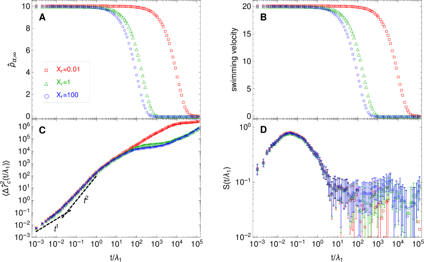
Figure 3: Effect of $X_{r}$ on the swimming dynamics. (A) Dimensionless concentration of the reactant in the bath, $\hat{\rho}_{\alpha,\infty}$. (B) Dimensionless swimming velocity. (C) Mean-squared displacement of the center of mass of the Janus swimmer. (D) Normalized cross-correlation between the orientation of the Janus swimmer, $\bm{Q}/Q$, and its instantaneous displacement vector, $\Delta\bm{r}(t)$. Other parameters were set to, $\hat{\ell_{0}}=1$, $X_{\lambda}:=D^{\prime}_{c\beta}/D^{\prime}_{c\alpha}=1$, $X_{S}=0.01$.

Fig. 3 shows the effect of $X_{r}:=\dfrac{k^{\prime\prime}}{D^{\prime}_{\alpha\alpha}\gamma_{\alpha\alpha\beta}}\sqrt{\dfrac{k_{\rm B}T}{k_{b}}}$ on the dynamics of the Janus dumbbell. As was discussed before $X_{r}$ is the ratio between a characteristic time scale for the mass transfer of reactants and a characteristic time scale of the chemical reaction. When $X_{r}>1$ the net reaction rate is limited by the mass transfer of reactant from the bath to the dumbbell. When $X_{r}<1$ the net reaction rate is mostly limited by the chemical reaction kinetics. Fig. 3A shows the dimensionless concentrations of the reactant for three different values of $X_{r}$ as a function of time. For $X_{r}=0.01$ the overall reaction rate is mostly limited by the chemical kinetics. For $X_{r}=1$ both mass transfer and reaction kinetics effects are important. While for $X_{r}=10$ the overall reaction rate is limited mainly by the mass transfer of reactant from the bath to the Janus dumbbell. In general, for lower values of $X_{r}$ the reaction rate is slower and therefore it takes longer for the reactant to be fully consumed and for the swimming velocity to decay to zero. Fig. 2C shows the effect of $X_{r}$ on the mean-squared displacement of the center of mass of the swimmer. As pointed out before, $\langle\Delta\hat{r}_{c}^{2}(t)\rangle$ exhibits four characteristic regions. A diffusive region is observed at short times with $\langle\Delta\hat{r}_{c}^{2}(t)\rangle\sim t^{1}$, this is followed by a ballistic region, where $\langle\Delta\hat{r}_{c}^{2}(t)\rangle\sim t^{2}$. In general, the ballistic region is followed by another diffusive region where the diffusivity of the dumbbell is larger than the diffusivity in the first diffusive region by a factor of about fifteen. At long times, when the reactant has been entirely depleted, another diffusive region that is completely thermal in nature can be observed. This diffusive region at long times exhibits a diffusivity that is smaller than the diffusivity observed in the intermediate diffusive region by a factor of about 30. For values of $X_{r}$ smaller than one, the diffusive region that appears at intermediate times and in which the dumbbell exhibits the largest diffusivity is longer than for values of $X_{r}$ larger than one. This is because for $X_{r}<1$ the net reaction rate is slower and the concentration of reactant remains larger than zero for a longer amount of time. In this intermediate diffusive region there is still a non-zero concentration of reactant in the bath but the swimmer can not maintain the ballistic motion due to tumbling, i.e reorientation of $\bm{Q}$ due to Brownian forces. However, as already pointed out the diffusivity of the dumbbell in this region can be larger than in the purely thermal diffusive region that appears at longer times by a factor of up to thirty. Fig. 3D shows the cross-correlation between the dumbbell’s orientation and its instantaneous displacement vector, $S(t)$. Again $S(t)$ exhibits a maximum at the same times at which $\langle\Delta\hat{r}_{c}^{2}(t)\rangle$ shows ballistic behavior. For all values of $X_{r}$ the ballistic behavior in the $\langle\Delta\hat{r}_{c}^{2}(t)\rangle$ and the maximum in $S(t)$ occur in the same time range, when $\rho_{\alpha,\infty}$ is still very large and the reaction rate is at its maximum .

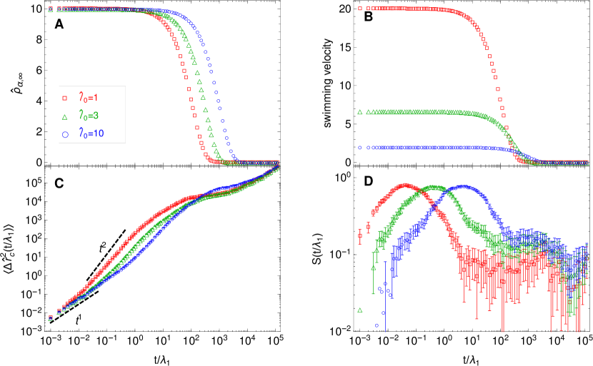
Figure 4: Effect of $\hat{\ell}_{0}$ on the swimming dynamics. (A) Dimensionless concentrations of the reactant in the bath, $\hat{\rho}_{\alpha,\infty}$. (B) Dimensionless swimming velocity. (C) Mean-squared displacement of the center of mass of the Janus swimmer. (D) Normalized cross-correlation between the orientation of the Janus swimmer, $\bm{Q}/Q$, and its instantaneous displacement vector, $\Delta\bm{r}(t)$. Other model parameters where set to, $X_{r}=10$, $X_{\lambda}:=D^{\prime}_{c\beta}/D^{\prime}_{c\alpha}=1$, $X_{S}=0.01$.

Figs. 4 and 5 show the effect of the rest length of the swimmer, $\ell_{0}$, on the swimming dynamics of the Janus dumbbell. Fig. 5 corresponds to a larger initial concentration of reactant and Fig. 4 is for a lower initial concentration of reactant. It can be observed in Figs. 4A and 5A that for smaller values of $\ell_{0}$ the reactant is consumed faster. That is because the concentration gradients around the swimmer are larger for shorter Janus dumbbells. These larger concentration gradients around the shorter dumbbells also produce larger swimming velocities as can be observed in Figs. 4B and 5B. This larger swimming velocities for the shorter Janus dumbbells are reflected in overall larger mean-squared displacements of their centers of mass. In Fig. 4C the mean-squared displacement of the center of mass of the swimmer again exhibits four distinct regions. A diffusive region at short times, followed by a ballistic region. Then a second diffusive region in which the swimmer’s diffusivity is larger than in the first diffusive region by a factor of about 15. When the concentration of reactant becomes very low, but is still finite, a plateau is observed. And finally, when the reactant is completely depleted, the diffusive region of purely thermal nature appears. In Fig. 5C it can be seen that when the initial concentration of reactant is made larger by a factor of ten the ballistic region in $\langle\Delta\hat{r}_{c}^{2}(t)\rangle$ broadens, and for the smaller values of $\ell_{0}$ the diffusive region at short times is not present.

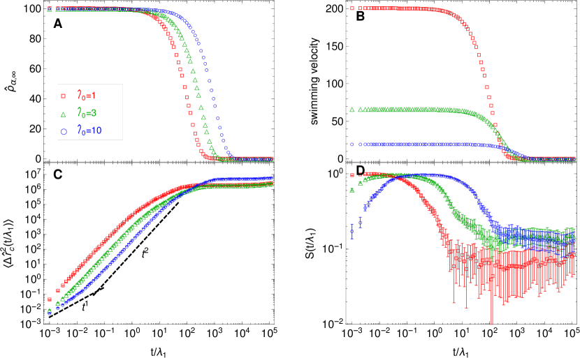
Figure 5: Effect of $\hat{\ell}_{0}$ on the swimming dynamics. (A) Dimensionless concentrations of the reactant in the bath, $\hat{\rho}_{\alpha,\infty}$. (B) Dimensionless swimming velocity. (C) Mean-squared displacement of the center of mass of the Janus swimmer. (D) Normalized cross-correlation between the orientation of the Janus swimmer, $\bm{Q}/Q$, and its instantaneous displacement vector, $\Delta\bm{r}(t)$. Other model parameters where set to, $X_{r}=10$, $X_{\lambda}:=D^{\prime}_{c\beta}/D^{\prime}_{c\alpha}=1$, $X_{S}=0.01$.

In Figs. 4D and 5D it can also be observed that the region at which $\langle\Delta\hat{r}_{c}^{2}(t)\rangle$ exhibits the ballistic region coincides with the region at which the cross-correlation between the orientation of the dumbbell, $\bm{Q}/Q$, and its instantaneous displacement vector exhibits a maximum. When $\ell_{0}$ is increased the ballistic region in $\langle\Delta\hat{r}_{c}^{2}(t)\rangle$ moves to longer times and so does the maxima in $S(t)$. Note that for the cases with larger initial concentration of reactant, shown in Fig. 5D, the maxima in $S(t)$ are much broader, encompassing several decades, this coincides with also a much broader ballistic region in the $\langle\Delta\hat{r}_{c}^{2}(t)\rangle$. Note also that in Fig. 4C due to the smaller values of the initial reactant bulk concentration, $\rho_{\alpha,\infty}(0)$, the plateau in the mean-squared displacement of the center of mass of the dumbbell is narrower compared to whats observed in Fig. 5C. This is because the total decoupling of the $\bm{r}_{c}(t)$ dynamics from the $\bm{Q}(t)$ dynamics due to reactant depletion occurs at shorter times for lower initial reactant concentrations. When $\rho_{\alpha,\infty}(0)$ is made ten times larger as shown in Fig. 5 this total decoupling takes more time and therefore the plateau in $\langle\Delta\hat{r}_{c}^{2}(t)\rangle$ is broader and the final diffusive region of purely thermal nature appears at longer times, that are not shown in the plot. Similar behavior in the mean squared displacement of the center of mass of diffusiophoretic microswimmers has also been observed in more detailed simulations ^{16, 3}. Moreover, more detailed simulations have also shown that the orientational correlation function attains its maximum value when the motion of the microswimmer is ballistic ¹⁶. An advantage of the the coarser model introduced in this work is that it allows for a wider window of time scales to be observed at a lower computational cost.

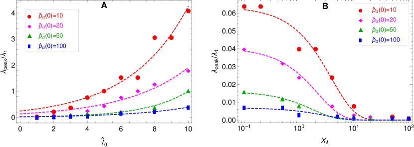
Figure 6: Time scales at which the cross-correlation between the orientation of the Janus swimmer, $\bm{Q}/Q$, and its instantaneous displacement vector, $\Delta\bm{r}(t)$, exhibits a maximum. (A) As a function of the dumbbell rest length, $\ell_{0}$, for different values of the the initial concentration of reactant in the bulk, $\rho_{\alpha,\infty}(0)$. Other parameters set to $X_{\lambda}:=D^{\prime}_{c\beta}/D^{\prime}_{c\alpha}=1$, $X_{r}=10$, $X_{S}=0.01$ (B) As a function of $X_{\lambda}:=D^{\prime}_{c\beta}/D^{\prime}_{c\alpha}$ for different values of the the initial concentration of reactant in the bulk, $\rho_{\alpha,\infty}(0)$. Other parameters set to $\hat{\ell}_{0}=1$, $X_{r}=10$, $X_{S}=0.01$.

The model presented here may be used as a tool when designing or analyzing experiments with Janus swimmers. For instance, Fig. 6 shows the time at which the cross-correlation between the orientation of the Janus dumbbell, $\bm{Q}/Q$, and its displacement vector, $\Delta\bm{r}_{c}$, exhibits a maximum, $\lambda_{\rm peak}$. This is the time at which the Janus dumbbell will exhibit swimming dynamics, or in other words the time at which it will be able to sustain ballistic motion with a persistent direction. The two model parameters, $\ell_{0}$ and $X_{\lambda}:=D^{\prime}_{c\beta}/D^{\prime}_{c\alpha}$, for which the location of the maximum in $S(t)$ exhibits dependence have been considered. Fig. 6A shows how the location of the maximum value of $S(t)$, $\lambda_{\rm peak}$, depends on the rest length of the dumbbell, $\ell_{0}$, for different values of the initial concentration of reactant in the bulk, $\rho_{\alpha,\infty}(0)$, for a system where $D^{\prime}_{c\alpha}$ and $D^{\prime}_{c\beta}$ are the same, i.e. $X_{\lambda}:=D^{\prime}_{c\beta}/D^{\prime}_{c\alpha}=1$. It can be observed that $\lambda_{\rm peak}$ increases exponentially as $\ell_{0}$ is increased and decreases exponentially as $\rho_{\alpha,\infty}(0)$ is increased. Longer swimmers produce smaller reactant gradients across their length and therefore are slower achieving swimming motion. The results in Fig. 6A can be collapsed into a single master curve, $\lambda_{\rm peak}/\lambda_{1}=0.3\exp\left({0.3\hat{\ell}_{0}}-0.05\hat{\rho}_{\alpha,\infty}(0)\right)$. In Fig. 6B the dependence of $\lambda_{\rm peak}$ on the ratio, $X_{\lambda}:=D^{\prime}_{c\beta}/D^{\prime}_{c\alpha}$, for different values of the the initial concentration of reactant in the bulk, for a system with $\hat{\ell}_{0}=1$ is illustrated. In this case, $\lambda_{\rm peak}$ decreases exponentially as $X_{\lambda}$ is increased. The swimming motion will occur at shorter times when $D^{\prime}_{c\beta}$ is larger than $D^{\prime}_{c\alpha}$. Or in other words, when the diffusivity of the reactant is smaller, the concentration gradients across the dumbbell are steeper and the swimming motion is observed at shorter times. However by comparing Fig. 6 A with Fig. 6 B is evident that the effect of $\ell_{0}$ on $\lambda_{\rm peak}$ is more pronounced than the effect of $X_{\lambda}$. The results in Fig. 6B can also be collapsed into a single master curve, $\lambda_{\rm peak}/\lambda_{1}=0.1\exp\left({-0.4X_{\lambda}}-0.04\hat{\rho}_{\alpha,\infty}(0)\right)$. These type of master curves could be helpful to rapidly determine the time scales at which swimming motion should be observable in an experiment for a given set of values of the initial reactant concentration, the swimmer’s size and/or diffusivity of reactants/products.

5 conclusions

In this manuscript a simple mean-field model for a Janus microswimmer has been proposed. The model was inspired by the nonequilibrium thermodynamics of multi-component fluids that undergo chemical reactions in the context of the GENERIC (general equation for the nonequilibrium reversible-irreversible coupling) framework. A Janus dumbbell was used to model the swimmer. The Janus dumbbell was assumed to be immersed in a bath of reactant. One of the beads of the dumbbell catalyzes a chemical reaction that consumes the reactant and produces a local gradient across the dumbbell’s orientation. The thermodynamic compliance of the swimmer model considered here can be rigorously but easily checked by tracking the entropy production rate of the closed system. Moreover simple evolution equations for the center of mass and the orientation of the Janus dumbbell were obtained.

The mass balance equations for the Janus swimmer were written in the phase space as a system of stochastic differential equations and Brownian dynamics simulations of the swimmer were performed. The simulations show that the simple mean-field swimmer model can exhibit ballistic motion when the concentration of reactant in the bath is large. Moreover, the cross-correlation between the direction of the swimmer’s motion and its orientation has a maximum at the same times at which the ballistic motion is observed. The mean-field Janus swimmer model has a small number of adjustable parameters. These are related to the diffusion coefficients of reactant and product, the rate constant for the surface reaction in the catalytic bead, the size of the beads and the rest length of the dumbbell. Moreover, the entropy balance for the model allows one to check that the entropy production rate stays positive for a given set of parameters. In this way it can be guaranteed that the the second law of thermodynamics is always obeyed in the simulations. In general, the simulations show that in the Janus dumbbell, the time scale at which swimming motion is observed increases exponentially with the dumbbell’s length and decreases exponentially with the ratio between the diffusivity of product and reactant. Moreover, reactions in which the product has larger diffusion coefficient than the reactant produce faster swimming. Also, shorter Janus swimmers produce steeper gradients across their lengths and will therefore swim faster than longer swimmers. The model presented here can help guide the design and analysis of experiments by providing fast estimates of the time scales at which swimming motion should be expected to be observed for a given system.

It is worth noting that the procedure that was followed in this work to obtain a mean-field Janus swimmer model for which the thermodynamics can systematically be checked can, in principle, also be extended to systems of several interacting swimmers. For instance, instead of assuming that the Janus dumbbell is in a bath of reactants and using the local gradient approximation used here it is also possible to keep the full mass balances for the reactants and products. That approach will require the evolution equations for the swimmer to be solved simultaneously with the full mass balance equations for the reactants and products.

Supplementary Material

Additional mathematical details to obtain the equations for the model used here are given in the supplementary information file.

References

- Oyama, Molina, and Yamamoto 2017 N. Oyama, J. J. Molina, and R. Yamamoto, “Simulations of model microswimmers with fully resolved hydrodynamics,” Journal of the Physical Society of Japan 86, 101008 (2017).
- Gomez-Solano et al. 2017 J. R. Gomez-Solano, S. Samin, C. Lozano, P. Ruedas-Batuecas, R. van Roij, and C. Bechinger, “Tuning the motility and directionality of self-propelled colloids,” Scientific reports 7, 14891 (2017).
- Lugli, Brini, and Zerbetto 2012 F. Lugli, E. Brini, and F. Zerbetto, “Shape governs the motion of chemically propelled janus swimmers,” The Journal of Physical Chemistry C 116, 592–598 (2012).
- Ebbens and Howse 2011 S. J. Ebbens and J. R. Howse, “Direct observation of the direction of motion for spherical catalytic swimmers,” Langmuir 27, 12293–12296 (2011).
- Michelin and Lauga 2015 S. Michelin and E. Lauga, “Autophoretic locomotion from geometric asymmetry,” The European Physical Journal E 38, 7 (2015).
- Wilson et al. 2013 D. A. Wilson, B. de Nijs, A. van Blaaderen, R. J. M. Nolte, and J. C. M. van Hest, “Fuel concentration dependent movement of supramolecular catalytic nanomotors,” Nanoscale 5, 1315–1318 (2013).
- Datt, Nasouri, and Elfring 2018 C. Datt, B. Nasouri, and G. J. Elfring, “Two-sphere swimmers in viscoelastic fluids,” Phys. Rev. Fluids 3, 123301 (2018).
- Yasuda et al. 2017 K. Yasuda, Y. Hosaka, M. Kuroda, R. Okamoto, and S. Komura, “Elastic three-sphere microswimmer in a viscous fluid,” Journal of the Physical Society of Japan 86, 093801 (2017).
- Nasouri, Khot, and Elfring 2017 B. Nasouri, A. Khot, and G. J. Elfring, “Elastic two-sphere swimmer in stokes flow,” Phys. Rev. Fluids 2, 043101 (2017).
- Milster et al. 2017 S. Milster, J. Nötel, I. M. Sokolov, and L. Schimansky-Geier, “Eliminating inertia in a stochastic model of a micro-swimmer with constant speed,” The European Physical Journal Special Topics 226, 2039–2055 (2017).
- Childress 2012 B. Sabass and U. Seifert, “Dynamics and efficiency of a self-propelled, diffusiophoretic swimmer,” The Journal of Chemical Physics 136, 064508 (2012a).
- Falasco et al. 2016 G. Falasco, R. Pfaller, A. P. Bregulla, F. Cichos, and K. Kroy, “Exact symmetries in the velocity fluctuations of a hot Brownian swimmer,” Phys. Rev. E 94, 030602 (2016).
- Golestanian, Liverpool, and Ajdari 2005 R. Golestanian, T. B. Liverpool, and A. Ajdari, “Propulsion of a molecular machine by asymmetric distribution of reaction products,” Physical review letters 94, 220801 (2005).
- Popescu et al. 2010 M. N. Popescu, S. Dietrich, M. Tasinkevych, and J. Ralston, “Phoretic motion of spheroidal particles due to self-generated solute gradients,” The European Physical Journal E 31, 351–367 (2010).
- Sabass and Seifert 2012b B. Sabass and U. Seifert, “Dynamics and efficiency of a self-propelled, diffusiophoretic swimmer,” The Journal of chemical physics 136, 064508 (2012b).
- Thakur and Kapral 2011 S. Thakur and R. Kapral, “Dynamics of self-propelled nanomotors in chemically active media,” The Journal of chemical physics 135, 024509 (2011).
- Krishnamurthy and Subramanian 2015 D. Krishnamurthy and G. Subramanian, “Collective motion in a suspension of micro-swimmers that run-and-tumble and rotary diffuse,” Journal of Fluid Mechanics 781, 422–466 (2015).
- Saintillan and Shelley 2008 D. Saintillan and M. J. Shelley, “Instabilities and pattern formation in active particle suspensions: kinetic theory and continuum simulations,” Physical Review Letters 100, 178103 (2008).
- Hernandez-Ortiz, Underhill, and Graham 2009 J. P. Hernandez-Ortiz, P. T. Underhill, and M. D. Graham, “Dynamics of confined suspensions of swimming particles,” Journal of Physics: Condensed Matter 21, 204107 (2009).
- Simha and Ramaswamy 2002 R. A. Simha and S. Ramaswamy, “Hydrodynamic fluctuations and instabilities in ordered suspensions of self-propelled particles,” Physical review letters 89, 058101 (2002).
- Brady and Bossis 1988 J. F. Brady and G. Bossis, “Stokesian dynamics,” Annual review of fluid mechanics 20, 111–157 (1988).
- Hernández-Ortiz, de Pablo, and Graham 2007 J. P. Hernández-Ortiz, J. J. de Pablo, and M. D. Graham, “Fast computation of many-particle hydrodynamic and electrostatic interactions in a confined geometry,” Physical review letters 98, 140602 (2007).
- Choudhary, Mandal, and Babu 2018 P. Choudhary, S. Mandal, and S. B. Babu, “Locomotion of a flexible one-hinge swimmer in stokes regime,” Journal of Physics Communications 2, 025009 (2018).
- Öttinger 2005 H. C. Öttinger, Beyond equilibrium thermodynamics (John Wiley & Sons, 2005).
- Grmela and Öttinger 1997 M. Grmela and H. C. Öttinger, “Dynamics and thermodynamics of complex fluids. I. Development of a general formalism,” Physical Review E 56, 6620 (1997).
- Öttinger and Grmela 1997 H. C. Öttinger and M. Grmela, “Dynamics and thermodynamics of complex fluids. II. Illustrations of a general formalism,” Physical Review E 56, 6633 (1997).
- Schieber 2003 J. D. Schieber, “Generic compliance of a temporary network model with sliplinks, chain-length fluctuations, segment-connectivity and constraint release,” Journal of Non-Equilibrium Thermodynamics 28, 179–188 (2003).
- Vázquez-Quesada, Ellero, and Español 2009 A. Vázquez-Quesada, M. Ellero, and P. Español, “Smoothed particle hydrodynamic model for viscoelastic fluids with thermal fluctuations,” Physical Review E 79, 056707 (2009).
- Wagner, Öttinger, and Edwards 1999 N. J. Wagner, H. C. Öttinger, and B. J. Edwards, “Generalized Doi–Ohta model for multiphase flow developed via generic,” AIChE journal 45, 1169–1181 (1999).
- Indei and Schieber 2017 T. Indei and J. D. Schieber, “Reexamination of multi-component non-ideal polymer solution based on the general equation for nonequilibrium reversible-irreversible coupling,” The Journal of Chemical Physics 146, 184902 (2017).
- Bird, Stewart, and Lightfoot 2007 R. Bird, W. Stewart, and E. Lightfoot, Transport Phenomena, revised 2 ed. (Wiley, 2007).
- Gardiner 2009 C. W. Gardiner, Stochastic Process, A handbook for the natural and social sciences, 4th ed. (Springer, New York, 2009).
- Öttinger 1996 H. C. Öttinger, Stochastic processes in polymeric fluids: tools and examples for developing simulation algorithms, 1st ed. (Springer, Berlin, Germany, 1996).