Effect of Antral Motility on Food Hydrolysis and Gastric Emptying from the Stomach: Insights from Computational Models

Abstract

The peristaltic motion of the stomach walls combines with the secretion of enzymes to initiate the process that breaks down food. Computational modelling of this phenomenon can help reveal the details that would be hard to capture via in-vivo or in-vitro means. In this study, the digestion of a liquid meal containing protein is simulated in a human-stomach model based on imaging data. Pepsin, the gastric enzyme for protein hydrolysis, is secreted from the proximal region of the stomach walls and allowed to react with the contents of the stomach. The jet velocities, the emptying rate, and the extent of hydrolysis are quantified for a control case, and also for three other cases of reduced motility with varying peristaltic amplitudes. The findings quantify the effect of motility on the rate of food breakdown and emptying, and correlate the observations with the mixing in the stomach induced by the antral contraction waves.

I Introduction

The human stomach stores, mixes, processes, and grinds ingested food. Understanding these functions is becoming increasingly important as issues related to digestion related disorders and nutrition are becoming prevalent Barnard (2010); Casini et al. (2015); Oberlander, Disdier, and Etilé (2017). For researchers in the field of medicine, stomach motility plays a key role in gastric disorders such as gastroesophageal reflux disease (GERD), gastroparesis (delayed emptying), dumping syndrome (rapid emptying), as well as in the pathophysiology of diabetes and functional dyspepsiaGrover, Farrugia, and Stanghellini (2019); Koch and Calles-Escandón (2015); Ukleja (2005); Mizuta et al. (2006), because the rate at which the stomach empties its contents affects the rate at which the nutrients get absorbed in the intestines. Gastric emptying is also important for drug delivery via oral administration as it determines the time it takes for effects of the drug to manifest themselves Lee et al. (2022). For researchers in the arena of nutrition and food design, a better understanding of the biomechanical processes involved in gastric digestion could help answer questions related to bioavailability of nutrients and the variation in emptying rates and food hydrolysis with food properties.

The physical and chemical action of the stomach is highly regional. The stomach has three major regions - the fundus, the corpus and the antrum. The fundus and corpus grow or shrink to accommodate the increasing volume of ingested food without increasing the pressure in the lumen. They also contain glands that secrete acid and enzymes to breakdown food Bornhorst (2017). The gastric pacemaker is also present along the greater curvature in the corpus. The pacemaker is responsible for initiating periodic peristaltic waves, known as antral contraction waves (ACWs), that travel aborally along the stomach walls. The amplitude of these waves is small in the region of inception but it rises gradually till the waves reach the antrum Pal et al. (2004); Schulze (2006). At the distal end of the antrum is the pylorus - a small orifice connecting the stomach to the duodenum. The orifice is surrounded by muscular tissues responsible for opening and closing the pylorus. Right before the ACWs terminate at the pylorus, a segmental contraction leads to a high-amplitude collapse of the walls; this event is known as the terminal antral contraction (TAC). TAC propels the trapped gastric contents away from the collapsing orifice and the coordination between the opening/closing of pylorus and the TAC is crucial to the dynamics of gastric emptyingIshida et al. (2019).

These muscular activities vary from meal-to-meal and person-to-person. Liquid meals are emptied much faster than solid meals Kelly (1980). Lower viscosity meals generate deeper indentation ACWs Koziolek et al. (2013) than higher viscosity ones. There also exists a feedback loop between the duodenum and the antrum that regulates the rate of caloric availability in the duodenum to about 2-4 kcal/min Brener, Hendrix, and McHugh (1983). The meal structure and softness plays a role in the emptying rate as well because the pyloric orifice ensures that only particles smaller than 2 mm are emptied while the rest continue to undergo fragmentation and dissolution within the antrum by the action of the retropulsive jet and the ACWs Schulze (2006). Thus, gastric mixing and emptying are complex processes with intricate neurohormonal control mechanisms that adjust the motility based on multiple food properties.

Studying the gastric chemo-fluid dynamics via experiments poses several challenges. In-vivo approaches are cost-intensive and ethically constrained. In-vitro models, on the other hand, fail to replicate the complex wall motion as well as the chemical response to the food Bornhorst and Paul Singh (2014). However, the stomach geometry and motility information gleaned from MRI scans can be used to construct computational (in-silico) models that overcome many of the limitations of these other approaches. This has become possible only in the recent decades with the advancement in computational power and algorithms.

There are relatively few examples of studies that have tried to investigate gastric mixing and emptying via computational models. The first work that used computational fluid dynamics (CFD) to investigate flow inside the stomach was based on a 2D stomach model Pal et al. (2004); Pal, Brasseur, and Abrahamsson (2007). Stomach motility was defined from in-vivo MRI data to study the rate of gastric emptying. Kozu et al. Kozu et al. (2010, 2014) studied the mixing of gastric contents in a simplified 2D model of the terminal antrum. An axisymmetric model was also developed by Alokaily et al. Alokaily, Feigl, and Tanner (2019) to study the effect of peristaltic wave parameters and viscosity on the retropulsive jet and recirculation of antral contents. Others have used full 3D stomach geometries as well Singh (2007); Ferrua and Singh (2010), in which simplified 3D geometric model of the stomach that was symmetric about the central plane was employed. In another study, the effect of posture on recirculation of gastric contents was investigated using an anatomically realistic geometry Imai et al. (2013). More recently, Ishida et al. Ishida et al. (2019) have investigated the effect of impairment of the coordination between ACW and the opening/closing of pylorus for meals with different viscosities. Li et al. Li and Jin (2021) studied the effect of TAC on the flow field and incorporated acid secretion into their model to understand pH variations inside the lumen. They also studied the stacking of food boluses due to foods of different densities Li et al. (2021). A recently described model has also incorporated fluid-structure interaction (FSI) between the fluid contents and the gastric muscle fibers Acharya et al. (2022).

Although the interest in this field is growing, computational models of gastric function lag far behind other disciplines such as cardiovascular and respiratory biomechanics. One key question that has not been addressed by the previous studies is the effect of stomach motility on the hydrolysis of food. Mixing in the stomach facilitates the chemical reaction between the enzymes and the ingested food, which determines the composition of the contents (“chyme”) emptied out of the stomach into the duodenum. The coupling of chemistry and fluid dynamics within the stomach is key to understanding the sites of enzymatic activity, effect of pH gradients, and the outcomes of impairment in stomach motility. Trusov et al. Trusov, Zaitseva, and Kamaltdinov (2016) carried out multi-species simulations of just the antro-duodenal region to investigate the effect of secretory function disorders but they did not focus on the effect of stomach motility on food breakdown. Furthermore, since the parietal cells and the chief cells, which secrete gastric enzymes, are located in the proximal stomach Bornhorst (2017), the complete stomach geometry is required to accurately capture the transport and activation of enzymes. A full stomach model that incorporates food hydrolysis will facilitate an understanding of the regional differences in enzymatic activity and how these differences evolve in time during gastric digestion..

The effect of stomach motility on gastric digestion can also be studied via computational models since these models allow us to systematically vary key parameters and exclude confounding effects. For example, stomach motility shows a wide variation in response to food properties but may also be affected by disease and dysfunction. Gastroparesis refers to delayed gastric emptying in the absence of any physical obstruction at the gastric outlet. In 2007, the age-adjusted prevalence of gastroparesis in the U.S. per 100,000 people was 24.2, a significant rise from 2.4 in the years 1996-2006 Grover, Farrugia, and Stanghellini (2019); Camilleri, Bharucha, and Farrugia (2011). It can be caused by diabetes, postsurgical or postinfection complications, but it is also idiopathic in a large subset of patients Grover, Farrugia, and Stanghellini (2019); Hereijgers et al. (2022). Variations in gastric motility can be caused by other conditions as well. For example, patients with Parkinson’s disease have slower gastric emptying and fewer antral contractions of smaller amplitude Hardoff et al. (2001); Bornhorst (2017). Erythromycin, which is a commonly used antibiotic, has been shown to improve antral contractility thereby increasing the ACW amplitudes Annese et al. (1992); Parkman et al. (1995). A computational model of gastric digestion could also be used to investigate on food mixing and breakdown.

In this study, we address: How do the enzymes secreted in the proximal stomach get mixed with the gastric contents and hydrolyze the ingested food? How does the composition of the contents emptied into the stomach change with time? How does this mixing, hydrolysis and emptying change with variations in gastric motility? In the past, our model has been used to study oral pill dissolution and API delivery into the intestines Seo and Mittal (2022); Lee et al. (2022). Here, we use it to model the hydrolysis of a liquid meal containing protein.

II Methodology

II.1 Stomach Model

The geometry of the stomach is obtained from the Virtual Population Library Gosselin et al. (2014) and is based on of the body type “Duke” which corresponds to a male adult. The pylorus and the duodenum are added manually using SolidWorks (Dassault Systèmes, Vélizy-Villacoublay, France) because they were not resolved clearly in available dataset. The duodenum is assumed to be a tubular extension with the same diameter as the antrum. The size of the pyloric opening, which is at the junction between the antrum and the duodenum, is critical for modelling the emptying rate. In the current study, this is modelled as a circular orifice of maximum opening size 2 mm based on existing literature on the post-prandial state of the stomach Meyer et al. (1988); Hellström, Grybäck, and Jacobsson (2006).

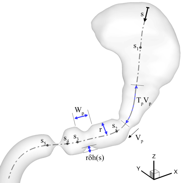
(a) Geometry and wall deformation model

(b) Amplitude modulation function along the centerline

Figure 1: Description of the stomach geometry and the motility model. The amplitude modulation function, $h(s)$, varies the strength of the ACWs along the centerline from 0 in fundus, to $\delta$ in antrum, and to $\delta A_{TAC}$ just before the pylorus.

Figure 2: The triangulated surface mesh is immersed in an outer Cartesian mesh with an open fundus at the top and an open duodenum at the bottom.

The amplitude of the ACW at any given axial location is given by $\delta\times h(s)$ where $\delta$ is the nominal strength of the ACWs. The amplitude modulation function $h(s)$ is a factor used to vary the effective strength of the ACWs from zero in the fundus (i.e. no ACW), to $\delta$ in the antrum, and then to $\delta A_{TAC}$ near the pylorus corresponding to the high amplitude collapse of walls due to terminal antral contraction (TAC). This variation, along with the stomach geometry describing the relevant motility parameters, is shown in Figure 1. The velocity, width and the occlusion of the ACWs were chosen from the literature and are described in Table 1.

Parameter	Value
$V_{p}$	2.3 mm/s
$W_{p}$	20 mm
$T_{p}$	20 s
$\delta$	0.4
$A_{TAC}$	2.0

Table 1: Motility model parameters based on Ferrua and SinghFerrua and Singh (2010). Other values of nominal amplitude of ACWs, $\delta$, were also considered ($\delta=$ 0.20, 0.27, 0.34) to model the weak motility state of the stomach.

II.2 Fluid Flow

The described stomach geometry and motility model is discretized with $\sim$ 33,000 triangular elements. The surface mesh is immersed into a Cartesian volume grid of size 24 cm $\times$ 8 cm $\times$ 16 cm in $x-$,$y-$ and $z-$direction, respectively, as shown in Figure 2, with a grid spacing of 0.5 mm in each direction.

The gastro-duodenal contents are assumed to have the properties of water (with density $\rho=1000$ kg/m³, and dynamic viscosity $\mu=0.001$ Pa s) which is a good assumption for liquid meals. The fluid flow is governed by the incompressible Navier-Stokes equations for Newtonian fluid:

$$\nabla\cdot\vec{u}=0;$$ (1)

$$\rho\left(\frac{\partial u}{\partial t}+\nabla\cdot\left(\vec{u}\vec{u}\right)\right)=-\nabla p+\mu\nabla^{2}\vec{u}+\rho\vec{g},$$ (2)

where $\vec{g}=-9.81$ m/s² $\hat{z}$ is acceleration due to gravity. A no-slip boundary condition is specified at the stomach lumen, and the geometry has two openings - one cutting through the fundus and another through the duodenum. The boundary condition (BC) on these two openings are specified based on the state of the pylorus. When the pylorus is open, the fundic boundary is closed by a zero-velocity BC and the duodenal boundary acts as an outflow with a zero-gradient BC for $\vec{u}$. When the pylorus is closed, the roles are switched - a no-slip BC is specified at the duodenal boundary and the fundic boundary has a zero-gradient BC. This allows small amounts of inflow or outflow from the corpus as would be expected for a incompressible flow.

The collapsing terminal antrum decreases the stomach volume when the pylorus is open, causing emptying of gastric contents through the pylorus and outflow via the open duodenum. The pylorus closes immediately before the completion of the collapse of terminal antrum. Subsequently, the antral relaxation raises the stomach volume back to its original value which pulls in more food from the fundus region. This flow behaviour acts as a model of tonic contractions that forces a net one-way flow through the pylorus. The rate of emptying is determined by the ACW kinematics and the fluid properties.

These equations are solved using ViCar3D, a sharp-interface immersed boundary method (IBM) solver Mittal et al. (2008). In this solver, the spatial derivatives are discretized using second-order central difference schemes, the equations are advanced in time using a fractional-step method, and the Crank-Nicolson scheme is used to integrate in time. A stabilized bi-conjugate gradient method is used to solve the pressure Poisson equation. More details on the numerical methodology and grid convergence study can be found in earlier works Lee et al. (2022); Seo and Mittal (2022).

II.3 Gastric Digestion Model

The chemical kinetics in a postprandial stomach are highly complex with different nutrients undergoing different chemical processing. The breakdown of carbohydrates, for example, begins in our mouth as mastication mixes our saliva with the food bolus. This continues till salivary amylase is exposed to the acidic environment of the stomach where it is deactivated Bornhorst and Singh (2012). The digestion of carbohydrates subsequently resumes in the small intestines. Proteins and lipids, on the other hand, are targeted by enzymes secreted from the gastric walls. The proximal gastric walls contain chief-cells that secrete pepsinogen and gastric lipase Bornhorst (2017). Pepsinogen is activated in the presence of acid to form pepsin which hydrolyzes proteins, while gastric lipase helps breakdown lipids. Each of these enzymes is highly sensitive to pH; pepsin’s activity is maximum at a pH of 2, and is completely inactive for pH$>$5; and gastric lipase on the the other hand shows peak activity in the pH range 5-6 Bornhorst (2017). The process is further complicated by other factors such as enzyme secretion rates that vary with the composition and physical properties of food as well as time elapsed since meal consumption. Thus, several assumptions need to be made to devise a model for the chemical breakdown of a liquid meal.

For this study, we focus on a single component liquid meal that only contains protein. Lipids are not considered in this model since they are lighter than water and add the extra complexity of gravity induced buoyancy effects. We further assume that the stomach has a constant pH at all times throughout the volume and the enzyme pepsinogen is instantaneously activated into pepsin upon entering the acidic environment of the stomach.

Protein hydrolysis is assumed to follow first-order catalytic reaction kinetics:

Protein $$+\quad \rightarrow\,\,\,\text{Hydro} +\quad \text{Pepsin};$$ Pepsin lyzed Protein (3)

(Food) (Enzyme) (Digesta) (Enzyme) (4)

There can be multiple varieties of proteins in a protein meal, and each type of protein exhibits a different reactivity with pepsin. The reaction constants for pepsin’s catalysis of each of these proteins are however not readily available. Here we assume that the ingested meal contains only one kind of protein - N-acetyl-L-phenylalanyl-L-phenylalanine ($C_{20}H_{22}N_{2}O_{4}$) - for which the reactivity with pepsin has been studied and the reaction constants at optimal pH value are available Cornish-Bowden, Greenwell, and Knowles (1969).

The three species in the model - pepsin, protein, and digesta - are modelled as passive scalars and an advection-diffusion-reaction equation is used to solve for their concentration:

$$\frac{\partial c_{i}}{\partial t}+\left(\vec{u}\cdot\nabla\right)c_{i}=D_{i}\nabla^{2}c_{i}+S_{i}$$ (5)

where $c_{i}$ is the concentration of $i^{th}$ species ($i=1,2,3$ correspond to pepsin, protein and digesta, respectively), $D_{i}$ is the diffusion coefficient of that species, and $S_{i}$ is the source term due to the digestion reaction. Given that the mixing in the postprandial stomach is advection dominated, we assume that each species has the same coefficient of diffusion $10^{-9}$ m²/s Trusov, Zaitseva, and Kamaltdinov (2016). Pepsin acts as a catalyst an therefore $S_{1}=0$. The source term due to the digestion reaction consumes protein, and produces digesta; therefore, $S_{2}=-S_{3}$ and following Cornish-Bowden, Greenwell, and Knowles (1969); Trusov, Zaitseva, and Kamaltdinov (2016), the value of this consumption/production rate is set to $k_{1}c_{2}c_{1}/(k_{2}+c_{2})$, $k_{1}=0.038/s$ where $c_{1},c_{2}$ represent the concentrations of pepsin and protein respectively, and $k_{2}=1.40\times 10^{-3}$ kmol/$m^{3}$.

To discretize the advection-diffusion equation, we use a second-order central-difference scheme for the diffusion terms, and a hybrid of second-order central and upwind schemes for the advection terms. A fourth-order Runge-Kutta method is used to explicitly integrate in time. At $t=0$, the stomach is filled with the homogeneous liquid meal, while the concentration of pepsin and digesta is set to zero. The concentration of protein in the meal is calculated based on a typical protein shake contents in the market - 24 g protein in 200 mL water. A zero mass-flux boundary condition is applied on the stomach walls for food and digesta. For pepsin, the flux on the proximal walls of the stomach is specified using the basal-pepsin-output (BPO) reported by Feldman et al. Feldman et al. (1996) . On the rest of the stomach walls, pepsin has a zero mass-flux. For all the species, a convective boundary condition is implemented at the duodenal outflow boundary, and a zero gradient condition is applied at the fundic boundary.

II.4 Simulating over long digestion times

The computational grid consists of $\sim$25 million points, which were required to resolve the flow through the pylorus and, at the same time, include the duodenum and entire stomach. Furthermore, simulating a few ACW cycles is not sufficient to capture the trends in meal breakdown. Even though the ACWs are initiated every 20 seconds, the process of gastric digestion might take anywhere from 30 min to several hours depending on the caloric density and other meal properties Koziolek et al. (2013). Each ACW cycle of 20 seconds takes $\sim$6000 hours of CPU time to simulate, and we are interested in digestion trends given by O(100) ACWs. This necessitates a computationally efficient approach to modelling the digestion. In the current simulations, we made use of the periodicity of the stomach kinematics and the flow inside the stomach model to enable simulation of digestion over O(100) ACWs at a considerably reduced computational expense.

We assume that the open fundus supplies the food that is emptied in each cycle and therefore, the volume of the stomach does not change with time. This assumption is valid for the early to mid stages of the digestion of a meal. The flow inside the stomach is therefore driven by the periodic motions of the ACW peristalsis and consequently, the fluid flow in this stomach achieves a periodic state within a few ACW cycles. The L₂-norm of the the difference between velocity field of the $3^{rd}$ cycle and the $4^{th}$ cycle, normalized by the velocity of the ACW, was O($10^{-7}$). In the current procedure, the simulated flow field for the 3rd cycle (roughly after about 40 seconds of ACW cycling) is recorded and subsequently, only the transport equation for pepsin, protein, and digesta are solved with this recorded velocity field. By eliminating the solving of the momentum and the mass conservation equations, we obtain a speed-up of 8.5 times and this enables us to simulate digestion for O(1000) seconds.

III Results

The development of computational models of the stomach is far behind that of cardiovascular flows. Only a few studies in the past have numerically investigated gastric fluid dynamics, and in this study we model the chemo-fluid dynamics of enzymatic hydrolysis of a liquid meal. Our aim is to investigate the effect of reduced motility (due to disease or medication) on the fluid flow as well as the rate of breakdown of liquid meal. The nominal amplitude of the antral contraction waves (ACWs) is varied from 0.4 (the control case) to 0.2 (the weakest motility case). The results are discussed in three parts - fluid flow, protein hydrolysis, and quantification of advective mixing. Then we end with a discussion on future work and the limitations of our current approach.

III.1 Fluid Flow

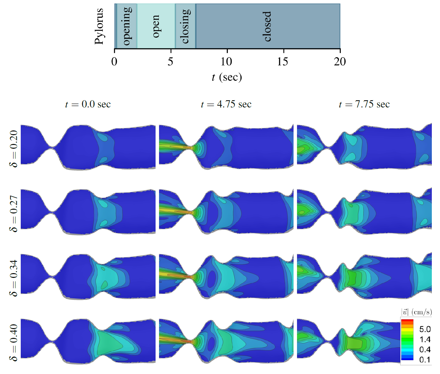
Figure 3: Comparison of velocity magnitude contours shown on a cross-section through the antro-duodenal region at three time instances - (1) $t=0.0:$ an ACW approaching an about-to-open pylorus, (2) $t=4.75:$ a fully open pylorus during the event of TAC, and (3) $t=7.75:$ right after the closing of pylorus. Notice that the TAC is still underway even after the pylorus has closed, which leads to a very prominent retrograde jet, specially in higher amplitude cases. Here $\delta$ is the fractional amplitude of the ACWs in the antrum, and the duodenum is to the left of the pylorus

Previous studies have described three key features inside the stomach that plan key roles in gastric mixing and emptying- a retropulsive jet, antral eddies between ACWs, and a pyloric jet. These flow features are reproduced in the current simulations as shown in Figure 3 which shows the velocity magnitude contours in the antrum on a plane that cuts through the centerline and the pyloric orifice. The retropulsive jet and the eddies between ACWs help transfer gastric contents away from the walls towards the center of the lumen and enhance mixing. The pyloric jet empties the contents into the duodenum while also entraining the pepsin into the jet, while the retropulsive jet transfers contents back into the stomach for further grinding and mixing. If the contents included solid food particles, the contents carried away by the retropulsive jet would contain all the solid particles larger than the pyloric orifice ($\sim$2 mm). This repeated grinding of food particles continues till particle size becomes smaller than the pyloric orifice, and the food can pass into the duodenum.

The time-sequence in Figure 3 illustrates the role of the phase between the pyloric sphincter and TAC, i.e., a collapse of the stomach walls right before the ACW terminates at the pylorus. Initially, an ACW approaches a closed pylorus and in this phase, the gastric contents are being transferred only to the proximal antrum via the retropulsive jet. As the ACW advances, the pylorus opens and a portion of the chyme trapped between the ACW and the pylorus empties via the pyloric orifice while a larger portion continues to be transported back into the stomach. This is when the TAC begins and increases the velocities of both jets. The pylorus closes before the TAC ends and the trapped chyme is, once again, left with only the retrograde path out of the collapsing segment. The retropulsive jet velocity peaks at this time while the pyloric jet velocity is maximum when the orifice was fully patent and the TAC had set in. The maximum area-averaged jet velocities of both jets are shown in Table 2. The pyloric jet velocities are an order-of-magnitude higher than the retropulsive jet velocities. Both, the retropulsive and pyloric, jet velocities also drop significantly with weakening motility. The retropulsive jet is however affected more adversely, dropping to 13% of the velocity of the control case, as compared to pyloric jet, which dropped only to 73%. This reveals that weakened motility implies significantly reduced gastric mixing tendencies.

Table 2: The peak velocity of the two jets is compared for different fractional amplitudes ($\delta$) of ACWs in the antrum. The % in parentheses is calculated by normalizing each case with the corresponding value of the control case ($\delta=0.4$).

$\delta$	Maximum Jet Velocity (cm/s)
	Retropulsive Jet	Pyloric Jet
0.20	0.24 (13%)	7.30 (73%)
0.27	0.43 (23%)	8.62 (86%)
0.34	0.83 (44%)	9.43 (94%)
0.40	1.88 (100%)	9.99 (100%)

The volume rate of emptying via the pyloric orifice is a key parameter because it influences the rate at which nutrients are absorbed in the intestines and it triggers the neurohormonal feedback mechanism Liu et al. (2021) that controls gastric motility. The emptying rate for different ACW amplitudes are shown in Table 3. The emptying rate drops by 35% for the case with the weakest motility.

Table 3: Comparison of the volume of fluid emptied through the pylorus per minute for different fractional amplitudes ($\delta$) of ACWs in the antrum. The % in parentheses is calculated by normalizing the emptying rate with that of the control case ($\delta=0.4$).

$\delta$	Emptying Rate (mL/min)
0.20	2.89 (65%)
0.27	3.61 (81%)
0.34	4.15 (93%)
0.40	4.48 (100%)

The case with $\delta=0.4$ has the same motility parameters used by Pal et al. Pal et al. (2004) and Ferrua and Singh Ferrua and Singh (2010), which are based on MRI data obtained after ingestion of 330 mL of meal with a caloric density of 0.73 kcal/mL. This case is used to validate the model by comparing the emptying rate of $\delta=0.40$ with other studies with a meal of a similar caloric density. As seen in Table 4, the emptying rate obtained from our computational model is close to experimental measurements by other studies of similar viscosity and caloric density meals.

Table 4: The emptying rate of current model is compared with other experimental works in the literature. The meal properties for present work correspond to the meal that was used in the imaging study whose motility parameters have been used in our model Pal et al. (2004); Ferrua and Singh (2010).

Study	Emptying Rate	Viscosity	Caloric Density
	(mL/min)	(Pa s)	(kcal/mL)
Present ($\delta=0.4$)	4.48	0.001	0.73
Marciani et al. Marciani et al. (2001)	4.1	0.06	0.64
Brener et al. Brener, Hendrix, and McHugh (1983)	4.26	“glucose solution”	0.5

III.2 Protein Hydrolysis

	$t=200s$	$t=400s$	$t=800s$	$t=2000s$	$t=4000s$
$\delta=0.20$
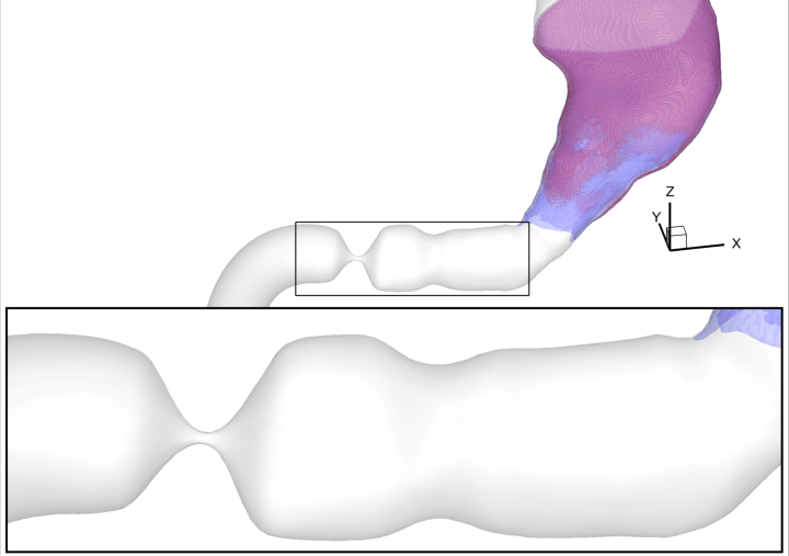
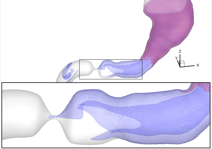
$\delta=0.27$
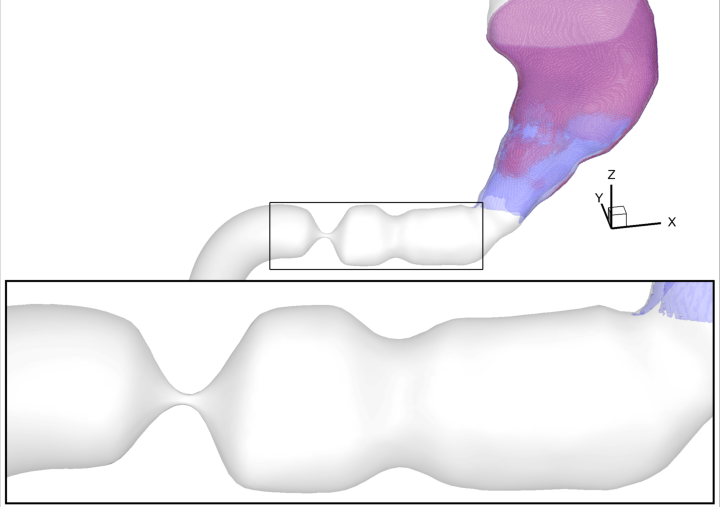
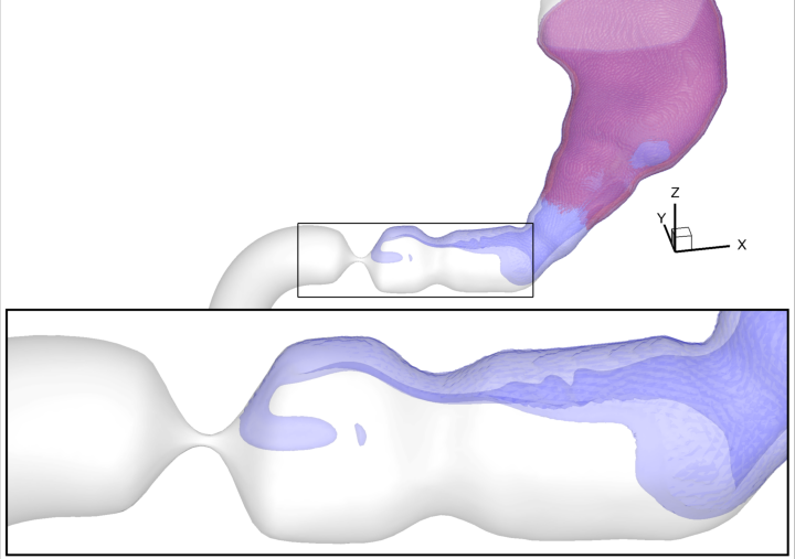
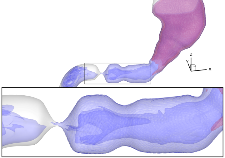
$\delta=0.34$
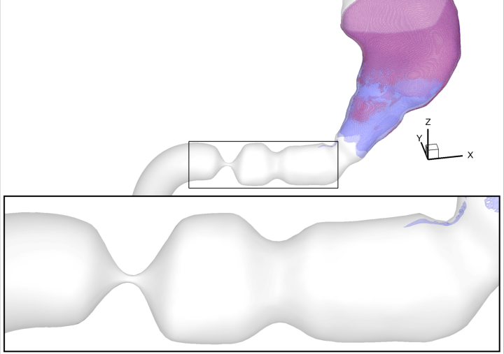
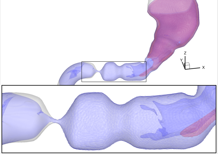
$\delta=0.40$

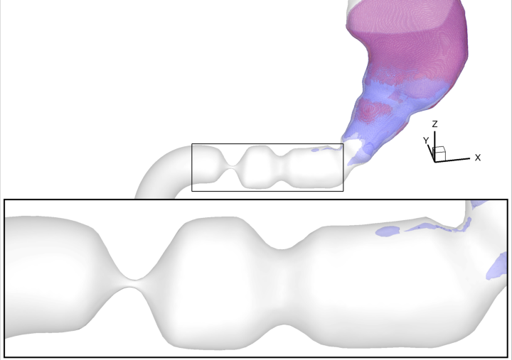
Figure 4: Iso-surfaces of concentration at level 0.01 (normalized with respect to the initial concentration of protein in the stomach) for pepsin (red), and digesta (blue) in the antral region. The meal fills the entire stomach at $t=0$ and $\delta$ corresponds to the fractional amplitude of the ACWs.

Figure 4 shows the progression of enzymatic hydrolysis of the protein-rich liquid meal for different amplitudes of ACW. The pepsin initiates the hydrolysis of the meal close to the secretion zones in the proximal stomach where the contents are relatively stagnant. Pepsin is subsequently transported away from the proximal walls by diffusion and also by advection in the corpus due to small amplitude ACWs that have originated in the mid-corpus. With these two mechanisms, the pepsin concentration front is slowly transported to the antrum along the stomach walls. The antrum has a much stronger advection due to the larger amplitude ACWs; this results in a significantly enhanced mixing as compared to the proximal stomach and leads to faster hydrolysis. The weaker motility cases take longer to transport pepsin from the proximal stomach to the antrum, and are also less efficient in mixing it with the protein once pepsin arrives in the antrum. Consequently, the rate of protein hydrolysis suffers as less protein is exposed to the enzyme. A detailed analysis of this mixing is done in the next section (III.3).

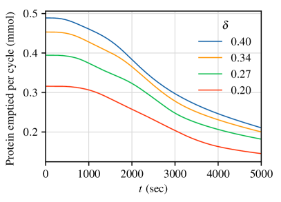
(a) Protein (Unhydrolyzed)

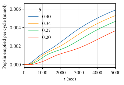
(b) Pepsin

Figure 5: Amount of (a) unhydrolyzed protein and (b) pepsin emptied per cycle for different cases.

As time progresses, pepsin continues to be secreted from the proximal walls and transported towards the antrum. The increase in amount of pepsin, combined with the fact that it is not consumed during the chemical reaction, causes the rate of digestion to rise exponentially in time. Eventually, this exponential rise slows down as pepsin starts to empty via the pylorus as well (as seen in figure 4) and an asymptote is reached when the amount of pepsin being secreted from the walls is matched by the rate of flux of pepsin through the pylorus. The chyme that empties via the pylorus is a mixture of undigested protein, pepsin, and hydrolyzed protein. Pepsin and undigested protein fluxes are represented by Figures 5. In the initial stages, almost no pepsin is emptied and most protein empties without being hydrolyzed. At later times, pepsin flux rises almost linearly but the protein flux drops because mixed pepsin starts hydrolyzing at an exponential rate. As we reach $t\sim 1$ hr, the exponential rate of hydrolysis starts to slow down and the protein flux starts to stagnate. During digestion, pepsin expelled into the duodenum gets deactivated because of the high pH environment in the duodenum, and from there, pancreatic proteases take over the digestion process Bornhorst and Paul Singh (2014).

Figure 6: Amount of digesta (hydrolyzed protein) emptied per cycle for different antral contraction wave (ACW) amplitudes. The symbols denote the total amount of hydrolyzed protein emptied every 20 sec from the simulations and the curves are obtained by fitting the modified Elashoff’s model to the simulation data.

The long duration (5000 seconds) over which the gastric hydrolysis is simulated allows us to capture the tri-phasic nature of gastric digestion as observed in Figure 6, which shows the amount of digesta emptied per cycle through the pylorus. It also shows that the poor mixing effect in fluid flow translates to the hydrolysis of the meal as well as weaker motility cases empty lesser amounts of digesta per cycle. However, for all cases, initially there is an exponential rise which changes into a linear growth that eventually asymptotes to a value as $t\rightarrow\infty$. The figure also shows trend lines obtained by fitting the modified Elashoff’s model, which has also been used by others to capture emptying of different gastric components Lee et al. (2022); Kong and Singh (2008); Siegel et al. (1988); Urbain et al. (1989). It is a sigmoid shape function given by:

$$A(t)=A_{\infty}(1-e^{-\alpha t})^{\beta},$$ (6)

where $A(t)$, in the current study, corresponds to the amount of digesta emptied per cycle (20 sec), $A_{\infty}$ is the predicted amount of digesta that would empty per cycle at steady state,and $\alpha$ and $\beta$ are time constants for emptying and initial delay in emptying, respectively. The parameters obtained after curve fitting are shown in Table 5. The parameter $A_{\infty}$ shows a uniform rise with $\delta$, also shown in Figure 7, which signifies that stronger motility leads to faster rate of hydrolysis and emptying of digesta. When the ACW amplitude is halved, the rate of hydrolysis at steady state dropped to 59% of its original value. $\alpha$ remains roughly the same over all choices of $\delta$ which means that the time constant of these curves is similar. The delay in the emptying rate is due to the time it takes to transport pepsin from secretion zones to the antrum. The rate of secretion of pepsin was the same for all cases but weaker amplitude ACWs are expected to be slower in transporting pepsin and show a longer delay. The interface length $\beta$ first decreases with rising $\delta$, and then remains roughly the same, then decreases again - which translates to weaker motility having a large delay period with a non-linear trend.

Table 5: Parameters obtained by fitting the modified Elashoff’s model to the digesta emptying rate in Figure 6 for different fractional amplitude of ACWs ($\delta$). Here $A_{\infty}$ is the predicted amount of digesta that would empty per cycle at steady state, $\alpha$ is the time constant of emptying, and $\beta$ is the initial delay in emptying, respectively.

$\delta$	$A_{\infty}$ (mmol)	$\alpha$ (sec-1)	$\beta$
0.20	0.19 (59%)	0.00070	4.30
0.27	0.24 (75%)	0.00068	3.84
0.34	0.29 (91%)	0.00070	3.93
0.40	0.32 (100%)	0.00067	3.55

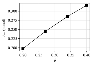
Figure 7: The amount of digesta emptied per cycle at steady state for different motility cases. This corresponds to the parameter $A_{\infty}$ obtained by fitting the Elashoff’s model to the pyloric emptying rate obtained from simulations.

III.3 Quantification of Advective Mixing

The chemical reaction occurs across the interface between the food and the enzyme, i.e. protein and pepsin. ACWs promote this reaction by stretching this interface and increasing the area across which the hydrolysis can occur and many of the observations and trends regarding the hydrolysis can be explained by examining evolution of the interface between food and enzyme for the various cases. A direct measure of the interface length or area, provides a direct measure of the mixing action of the ACWs and we choose to calculate the interface for pepsin because it is the only component that is not being consumed or produced in the proteolytic process. The procedure to calculate the interface length is mentioned in brief in the appendix (B), but a detailed explanation of the calculation can be found in a previous work Rips and Mittal (2019). The procedure results in an interface length field variable $\xi$ which has values of 0, $\Delta$ or $\sqrt{2}\Delta$ for each grid cell, where $\Delta$ is the linear dimension of a grid cell. This interface length field is is visualized in Figure 8 for one plane ($s=16$) at $t=1$ hr.

Figure 8: Calculating the interface at a cross-section through the antrum for $\delta=0.4$ case at $t=1$ hr. (a) A plane normal to the centerline in the antrum ($s=16$), (b) contours of pepsin concentration on that plane, (c) contours of normalized concentration gradient, (d) the interface, $\xi$, formed by the local peaks in this gradient.

Figure 9 compares the interface at $x=12$ at $t=1$ hr for the four motility cases. It is clear that the reaction interface is more widespread in the higher motility cases, which is a consequence of better mixing of pepsin with the contents. The inability to mix pepsin thoroughly results in almost non-existent reaction sites at the center of the lumen. On the other hand, stronger motility exhibits intertwined and layered interfaces which fill the entire lumen.

Figure 9: Reaction interfaces for different motility amplitudes ($\delta$) at $t=1$ hr at a plane perpendicular to the centerline in the antrum at $s=16$. The enhanced mixing of high amplitude cases translates to a denser distribution of reaction fronts.

The sum of $\xi$ over the cross-section plane normalized by maximum possible length of the interface at the cross-section gives us the interface length ($L_{i}$), i.e.,

$$L_{i}=\dfrac{\sum\limits_{i,j=1}^{N_{1},N_{2}}\xi(i,j)}{L_{max}}\\$$ (7)

where, $L_{max}=N_{1}\times N_{2}\times\Delta$ is an upper bound on the possible interface length at any cross-section, $N_{1}$ and $N_{2}$ are the grid points inside the lumen in the two orthogonal directions, and $\Delta$ is the grid size. So, $L_{i}$ denotes the fraction of the lumen that is filled by the interface. The variation of the interface length along the centerline, starting from $s=0$ (at the top of the fundus) to $s=20$ (right before the pylorus), is shown in Figure 10. This figure demonstrates that all cases exhibit similar advective mixing in the fundus, but the interface lengths start to become quite different in the antrum region. This is because there is no wall motion in the fundus region, and the pepsin distribution in that region is similar for all cases.

(a)

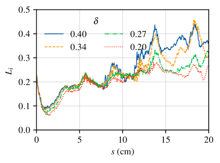
(b)

Figure 10: The normalized area integral of $\xi$ on the cross-section planes gives interface length, $L_{i}$. This figure shows its comparison for different motility cases at $t=1$ hr from the fundus to the terminal antrum.

To see how the interface changes in time, we integrate the interface length along the centerline in the antrum region ($12\leq s\leq 20$) and normalize it by the length of the centerline to end up with a single value at each time step, termed as interface area ($A_{i}$). Mathematically,

$$A_{i}=\frac{\int L_{i}ds}{\int ds}.$$ (8)

The variation of interface area is shown in Figure 11. This area is a measure of the size of the pepsin’s concentration front and quantifies how well it is mixed in with the contents of the stomach. There is a transience period after which all cases stabilize to a constant value. It is noted that high ACW amplitude cases not only have a shorter transience time but a significantly higher overall interface area. Furthermore, to quantify the steady state behavior, the value of interface area after an hour for each case is also shown.

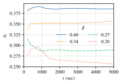
(a)

(b)

Figure 11: (a) Interface area of pepsin is shown as a function of time. After initial transience, the interface area stabilizes to a constant value that quantifies how well is pepsin mixed with the gastric contents. (b) The reaction interface area at $t=1$ hr is compared for different motility cases

The current model provides new data and insights for gastric mixing and food breakdown, but has several limitations. First, the stomach volume is held constant over the entire duration of 5000 seconds simulated here. This assumes that the fundus has sufficient meal content stored that it can keep supplying small amounts over time to maintain the stomach volume. This assumption made it computationally tractable to capture hydrolysis trends over a long enough digestion period. The model also assumed a uniform pH throughout the stomach volume and this translates to instant activation of pepsinogen into pepsin. In an actual stomach, the importance of acid secretion and pH microclimates in enzyme activation is expected to be important. We expect the digestion delay phase to last longer if we consider the effect of pH as well.

Notwithstanding these limitations, the current model allows us to quantify the effects of disorders like gastroparesis on food hydrolysis. We have quantified advective mixing within the stomach and how this mixing is modulated by changes in antral motility. All this information would be extremely challenging to obtain in an experimental setting. We were also able extend the simulations to long durations and capture trends over a time period that is comparable to actual digestion time scale. In future work, we plan to include the effect of meal properties and tonic contractions of the stomach in our models. These features will make this model more complete and viable for a wider range of gastric digestion scenarios.

Data Availability Statement

The data that support the findings of this study are available from the corresponding author upon reasonable request.

Appendix A Stomach Motility

Stomach motility is defined in a manner similar to the model of Ferrua and Singh Ferrua and Singh (2010). The peristaltic contractions, known as antral contraction waves (ACWs), deform the walls towards the centerline and propagate distally - from the upper body of the stomach towards the pylorus. The deformation was defined as:

$$\vec{x}_{w}=\vec{x}_{w,0}+\lambda\vec{r}_{w},$$ (9)

where $\vec{x}_{w}$ is the position vector of any point on the wall, $\vec{x}_{w,0}$ is the initial position vector of the point without any deformation, $\lambda$ is the fractional change in the radius, and $\vec{r}_{w}$ is a vector from the point on the wall towards the centerline. $\lambda$ is given by:

$$\lambda(t,s)=\delta h(s)\sum_{n}\frac{F(s,s_{0,n})}{2}\left(\cos\left(2\pi\frac{s-s_{0,n}}{W_{p}}\right)+1\right),$$ (10)

where $s$ is the distance along the centerline, $\delta$ corresponds to the nominal deformation due to the wave, $h(s)$ is the amplitude modulation function which is used to vary the strength of this deformation along the centerline, $n$ is the wave count, $s_{0,n}$ is the location of $n^{th}$ wave, $F(s,s_{0,n})$ is the filter function that restricts the deformation to half-wave-width distance from the center of each wave, and $W_{p}$ is the width of the wave.

That amplitude modulation function and filter function are given by:

$$F(s,s_{0,n})=\left\{\begin{array}[]{ll}1&\mbox{if }|s-s_{0,n}|\leq W_{p}/2,\\ 0&\mbox{otherwise, }\end{array}\right.$$ (11)

$$h(s)=\left\{\begin{array}[]{ll}0&\mbox{if }s\leq s_{1},\\ \frac{1}{2}\left(1-\cos(\pi\frac{s-s_{1}}{s_{2}-s_{1}})\right)&\mbox{if }s_{1}<s\leq s_{2},\\ 1&\mbox{if }s_{2}<s\leq s_{3},\\ \frac{A_{TAC}-1}{2}\left(1-\cos(\pi\frac{s-s_{3}}{s_{4}-s_{3}})\right)&\mbox{if }s_{3}<s\leq s_{4},\\ \frac{A_{TAC}}{2}\left(1+\cos(\pi\frac{s-s_{4}}{s_{pyl}-s_{4}})\right)&\mbox{if }s_{4}<s\leq s_{pyl},\\ 0&\mbox{if }s_{pyl}<s,\end{array}\right.$$ (12)

$$s_{0,n}=V_{p}t+nT_{p}V_{p}\mbox{ and }s_{pyl}=\left(s_{4}+s_{5}\right)/2,$$ (13)

where $s_{1}$ to $s_{5}$ are locations along the centerline, $s_{pyl}$ is the location of the pylorus, $A_{TAC}$ is the factor that controls the strength of collapse of the terminal antrum due to TAC, $V_{p}$ is the speed of propagation of the ACW, and $T_{p}$ is the time interval between two subsequent ACWs.

Appendix B Calculating Interface

To identify the interface of pepsin, we consider planes passing normal to the stomach centerline. On each plane, we calculate the concentration gradient and then normalize it by the $L_{\infty}$-norm, i.e. $\nabla c/|\nabla c|_{\infty}$. We then find local peaks in this normalized gradient over the plane to identify the interface $\xi$. If the normalized gradient of a cell is greater than two of its immediate neighbours (north, south, east, and west), then $\xi=\Delta$. If the normalized gradient value is greater than all four of its neighbours, then $\xi=\sqrt{2}\Delta$. Each step of this procedure is visualised in Figure 12 at one plane at $t=1$ hr. The generated $\xi$ field inside the stomach identifies the concentration front of pepsin. Similar approach has been used in a previous work by Rips and Mittal Rips and Mittal (2019).

Figure 12: The procedure for calculating interface, $\xi$, at a plane perpendicular to the $yz$-plane at $x=12$. (a) The concentration of pepsin on the plane, (b) normalized concentration gradient, (c) local peaks in the gradient over the plane give the interface, (d) zoomed into the inset with visible grid lines.

References

- Barnard (2010) N. D. Barnard, “Trends in food availability, 1909–2007,” The American Journal of Clinical Nutrition 91, 1530S–1536S (2010).
- Casini et al. (2015) L. Casini, C. Contini, C. Romano, and G. Scozzafava, “Trends in food consumptions: What is happening to generation X?” British Food Journal 117, 705–718 (2015).
- Oberlander, Disdier, and Etilé (2017) L. Oberlander, A.-C. Disdier, and F. Etilé, “Globalisation and national trends in nutrition and health: A grouped fixed-effects approach to intercountry heterogeneity: Globalisation and the nutrition transition,” Health Economics 26, 1146–1161 (2017).
- Grover, Farrugia, and Stanghellini (2019) M. Grover, G. Farrugia, and V. Stanghellini, “Gastroparesis: A turning point in understanding and treatment,” Gut 68, 2238–2250 (2019).
- Koch and Calles-Escandón (2015) K. L. Koch and J. Calles-Escandón, “Diabetic Gastroparesis,” Gastroenterology Clinics 44, 39–57 (2015).
- Ukleja (2005) A. Ukleja, “Dumping Syndrome: Pathophysiology and Treatment,” Nutrition in Clinical Practice 20, 517–525 (2005).
- Mizuta et al. (2006) Y. Mizuta, S. Shikuwa, H. Isomoto, R. Mishima, Y. Akazawa, J.-i. Masuda, K. Omagari, F. Takeshima, and S. Kohno, “Recent insights into digestive motility in functional dyspepsia,” Journal of Gastroenterology 41, 1025–1040 (2006).
- Lee et al. (2022) J. H. Lee, S. Kuhar, J. H. Seo, P. J. Pasricha, and R. Mittal, “Computational modeling of drug dissolution in human stomach: Effects of posture and gastroparesis on drug bioavailability,” Physics of Fluids , 5.0096877 (2022).
- Bornhorst (2017) G. M. Bornhorst, “Gastric Mixing During Food Digestion: Mechanisms and Applications,” Annual Review of Food Science and Technology 8, 523–542 (2017).
- Pal et al. (2004) A. Pal, K. Indireshkumar, W. Schwizer, B. Abrahamsson, M. Fried, and J. G. Brasseur, “Gastric flow and mixing studied using computer simulation,” Proceedings of the Royal Society of London. Series B: Biological Sciences 271, 2587–2594 (2004).
- Schulze (2006) K. Schulze, “Imaging and modelling of digestion in the stomach and the duodenum,” Neurogastroenterology & Motility 18, 172–183 (2006).
- Ishida et al. (2019) S. Ishida, T. Miyagawa, G. O’Grady, L. K. Cheng, and Y. Imai, “Quantification of gastric emptying caused by impaired coordination of pyloric closure with antral contraction: A simulation study,” Journal of The Royal Society Interface 16, 20190266 (2019).
- Kelly (1980) K. A. Kelly, “Gastric emptying of liquids and solids: Roles of proximal and distal stomach,” American Journal of Physiology-Gastrointestinal and Liver Physiology 239, G71–G76 (1980).
- Koziolek et al. (2013) M. Koziolek, G. Garbacz, M. Neumann, and W. Weitschies, “Simulating the Postprandial Stomach: Physiological Considerations for Dissolution and Release Testing,” Molecular Pharmaceutics 10, 1610–1622 (2013).
- Brener, Hendrix, and McHugh (1983) W. Brener, T. R. Hendrix, and P. R. McHugh, “Regulation of the Gastric Emptying of Glucose,” Gastroenterology 85, 76–82 (1983).
- Bornhorst and Paul Singh (2014) G. M. Bornhorst and R. Paul Singh, “Gastric Digestion In Vivo and In Vitro: How the Structural Aspects of Food Influence the Digestion Process,” Annual Review of Food Science and Technology 5, 111–132 (2014).
- Pal, Brasseur, and Abrahamsson (2007) A. Pal, J. G. Brasseur, and B. Abrahamsson, “A stomach road or “Magenstrasse” for gastric emptying,” Journal of Biomechanics 40, 1202–1210 (2007).
- Kozu et al. (2010) H. Kozu, I. Kobayashi, M. Nakajima, K. Uemura, S. Sato, and S. Ichikawa, “Analysis of Flow Phenomena in Gastric Contents Induced by Human Gastric Peristalsis Using CFD,” Food Biophysics 5, 330–336 (2010).
- Kozu et al. (2014) H. Kozu, I. Kobayashi, M. A. Neves, M. Nakajima, K. Uemura, S. Sato, and S. Ichikawa, “PIV and CFD studies on analyzing intragastric flow phenomena induced by peristalsis using a human gastric flow simulator,” Food & Function 5, 1839–1847 (2014).
- Alokaily, Feigl, and Tanner (2019) S. Alokaily, K. Feigl, and F. X. Tanner, “Characterization of peristaltic flow during the mixing process in a model human stomach,” Physics of Fluids 31, 103105 (2019).
- Singh (2007) S. K. Singh, Fluid Flow and Disintegration of Food in Human Stomach, Ph.D. thesis, University of California, Davis, United States – California (2007).
- Ferrua and Singh (2010) M. Ferrua and R. Singh, “Modeling the Fluid Dynamics in a Human Stomach to Gain Insight of Food Digestion,” Journal of Food Science 75, R151–R162 (2010).
- Imai et al. (2013) Y. Imai, I. Kobayashi, S. Ishida, T. Ishikawa, M. Buist, and T. Yamaguchi, “Antral recirculation in the stomach during gastric mixing,” American Journal of Physiology-Gastrointestinal and Liver Physiology 304, G536–G542 (2013).
- Li and Jin (2021) C. Li and Y. Jin, “A CFD model for investigating the dynamics of liquid gastric contents in human-stomach induced by gastric motility,” Journal of Food Engineering 296, 110461 (2021).
- Li et al. (2021) C. Li, J. Xiao, X. D. Chen, and Y. Jin, “Mixing and emptying of gastric contents in human-stomach: A numerical study,” Journal of Biomechanics 118, 110293 (2021).
- Acharya et al. (2022) S. Acharya, S. Halder, W. Kou, P. J. Kahrilas, J. E. Pandolfino, and N. A. Patankar, “A fully resolved multiphysics model of gastric peristalsis and bolus emptying in the upper gastrointestinal tract,” Computers in Biology and Medicine 143, 104948 (2022).
- Trusov, Zaitseva, and Kamaltdinov (2016) P. V. Trusov, N. V. Zaitseva, and M. R. Kamaltdinov, “A Multiphase Flow in the Antroduodenal Portion of the Gastrointestinal Tract: A Mathematical Model,” Computational and Mathematical Methods in Medicine 2016, 1–18 (2016).
- Camilleri, Bharucha, and Farrugia (2011) M. Camilleri, A. E. Bharucha, and G. Farrugia, “Epidemiology, Mechanisms, and Management of Diabetic Gastroparesis,” Clinical Gastroenterology and Hepatology 9, 5–12 (2011).
- Hereijgers et al. (2022) M. J. M. Hereijgers, D. Keszthelyi, J. W. Kruimel, A. A. M. Masclee, and J. M. Conchillo, “Antroduodenal motility recording identifies characteristic patterns in gastroparesis related to underlying etiology,” Neurogastroenterology & Motility , e14394 (2022).
- Hardoff et al. (2001) R. Hardoff, M. Sula, A. Tamir, A. Soil, A. Front, S. Badarna, S. Honigman, and N. Giladi, “Gastric emptying time and gastric motility in patients with Parkinson’s disease,” Movement Disorders 16, 1041–1047 (2001).
- Annese et al. (1992) V. Annese, J. Janssens, G. Vantrappen, J. Tack, T. L. Peeters, P. Willemse, and E. Van Cutsem, “Erythromycin accelerates gastric emptying by inducing antral contractions and improved gastroduodenal coordination,” Gastroenterology 102, 823–828 (1992).
- Parkman et al. (1995) H. P. Parkman, A. P. Pagano, M. A. Vozzelli, and J. P. Ryan, “Gastrokinetic effects of erythromycin: Myogenic and neurogenic mechanisms of action in rabbit stomach,” American Journal of Physiology-Gastrointestinal and Liver Physiology 269, G418–G426 (1995).
- Seo and Mittal (2022) J. H. Seo and R. Mittal, “Computational Modeling of Drug Dissolution in the Human Stomach,” Frontiers in Physiology 12 (2022).
- Gosselin et al. (2014) M.-C. Gosselin, E. Neufeld, H. Moser, E. Huber, S. Farcito, L. Gerber, M. Jedensjö, I. Hilber, F. D. Gennaro, B. Lloyd, E. Cherubini, D. Szczerba, W. Kainz, and N. Kuster, “Development of a new generation of high-resolution anatomical models for medical device evaluation: The Virtual Population 3.0,” Physics in Medicine and Biology 59, 5287–5303 (2014).
- Meyer et al. (1988) J. Meyer, J. Elashoff, V. Porter-Fink, J. Dressman, and G. Amidon, “Human postprandial gastric emptying of 1–3-millimeter spheres,” Gastroenterology 94, 1315–1325 (1988).
- Hellström, Grybäck, and Jacobsson (2006) P. M. Hellström, P. Grybäck, and H. Jacobsson, “The physiology of gastric emptying,” Best Practice & Research Clinical Anaesthesiology Pre-Operative Fasting, 20, 397–407 (2006).
- Mittal et al. (2008) R. Mittal, H. Dong, M. Bozkurttas, F. Najjar, A. Vargas, and A. von Loebbecke, “A versatile sharp interface immersed boundary method for incompressible flows with complex boundaries,” Journal of Computational Physics 227, 4825–4852 (2008).
- Bornhorst and Singh (2012) G. M. Bornhorst and R. P. Singh, “Bolus Formation and Disintegration during Digestion of Food Carbohydrates,” Comprehensive Reviews in Food Science and Food Safety 11, 101–118 (2012).
- Cornish-Bowden, Greenwell, and Knowles (1969) A. J. Cornish-Bowden, P. Greenwell, and J. R. Knowles, “The rate-determining step in pepsin-catalysed reactions, and evidence against an acyl-enzyme intermediate,” Biochemical Journal 113, 369–375 (1969).
- Feldman et al. (1996) M. Feldman, B. Cryer, K. E. McArthur, B. A. Huet, and E. Lee, “Effects of aging and gastritis on gastric acid and pepsin secretion in humans: A prospective study,” Gastroenterology 110, 1043–1052 (1996).
- Liu et al. (2021) W. Liu, Y. Jin, P. J. Wilde, Y. Hou, Y. Wang, and J. Han, “Mechanisms, physiology, and recent research progress of gastric emptying,” Critical Reviews in Food Science and Nutrition 61, 2742–2755 (2021).
- Marciani et al. (2001) L. Marciani, P. A. Gowland, R. C. Spiller, P. Manoj, R. J. Moore, P. Young, and A. J. Fillery-Travis, “Effect of meal viscosity and nutrients on satiety, intragastric dilution, and emptying assessed by MRI,” American Journal of Physiology-Gastrointestinal and Liver Physiology 280, G1227–G1233 (2001).
- Kong and Singh (2008) F. Kong and R. Singh, “Disintegration of Solid Foods in Human Stomach,” Journal of Food Science 73, R67–R80 (2008).
- Siegel et al. (1988) J. A. Siegel, J. L. Urbain, L. P. Adler, N. D. Charkes, A. H. Maurer, B. Krevsky, L. C. Knight, R. S. Fisher, and L. S. Malmud, “Biphasic nature of gastric emptying.” Gut 29, 85–89 (1988).
- Urbain et al. (1989) J.-L. Urbain, J. Siegel, N. Charkes, A. Maurer, L. Malmud, and R. Fisher, “The two-component stomach: Effects of meal particle size on fundal and antral emptying,” European Journal of Nuclear Medicine 15 (1989), 10.1007/BF00257543.
- Rips and Mittal (2019) A. Rips and R. Mittal, “Flutter-enhanced mixing in small-scale mixers,” Physics of Fluids 31, 107107 (2019).
- Towns et al. (2014) J. Towns, T. Cockerill, M. Dahan, I. Foster, K. Gaither, A. Grimshaw, V. Hazlewood, S. Lathrop, D. Lifka, G. D. Peterson, R. Roskies, J. R. Scott, and N. Wilkins-Diehr, “XSEDE: Accelerating Scientific Discovery,” Computing in Science & Engineering 16, 62–74 (2014).