RIS-Aided Angular-Based Hybrid Beamforming Design in mmWave Massive MIMO Systems

Abstract

This paper proposes a reconfigurable intelligent surface (RIS)-aided and angular-based hybrid beamforming (AB-HBF) technique for the millimeter wave (mmWave) massive multiple-input multiple-output (MIMO) systems. The proposed RIS-AB-HBF architecture consists of three stages: (i) RF beamformer, (ii) baseband (BB) precoder/combiner, and (iii) RIS phase shift design. First, in order to reduce the number of RF chains and the channel estimation overhead, RF beamformers are designed based on the 3D geometry-based mmWave channel model using slow time-varying angular parameters of the channel. Second, a BB precoder/combiner is designed by exploiting the reduced-size effective channel seen from the BB stages. Then, the phase shifts of the RIS are adjusted to maximize the achievable rate of the system via the nature-inspired particle swarm optimization (PSO) algorithm. Illustrative simulation results demonstrate that the use of RISs in the AB-HBF systems has the potential to provide more promising advantages in terms of reliability and flexibility in system design.

I Introduction

In envisioned sixth-generation (6G) wireless communication systems, enormously abundant spectrum at high frequencies is needed to be exploited in order to support eccentric applications which impose extreme performance requirements [1]. Although millimeter-wave (mmWave) transmission is one of the cornerstones of fifth-generation (5G) and beyond communication systems, promising technologies such as massive multiple-input multiple-output (MIMO) and reconfigurable intelligent surface (RIS) have been introduced to combat the high path loss and blockage susceptibility at these frequencies [2, 3, 4]. RISs, which are composed of a low-cost and passive reflecting elements, have recently attracted great interest by both academia and industry to improve the capacity and the transmission performance of wireless communication systems [5, 6, 7].

Beamforming (i.e., precoding in transmission and combining in reception) is an essential signal processing technique to ensure reliable communications between the transmitter and receiver. Although the conventional MIMO systems widely considers single-stage fully-digital beamforming, it causes two crucial challenges for the massive MIMO systems: (i) high hardware cost due to a single dedicated power-hungry radio frequency (RF) chain per antenna, (ii) large channel estimation overhead size [8]. Hybrid beamforming (HBF) is introduced as a promising solution, which interconnects analog RF-stage and digital baseband (BB)-stage via employing limited number of RF chains [9]. Furthermore, in [10, 11, 12], angular-based HBF (AB-HBF) is developed for also reducing the instantaneous channel estimation overhead size. Particularly, it builds RF-stage via slow time-varying angular information and BB-stage via reduced dimensional channel state information (CSI).

Recently, RIS-assisted HBF studies have been introduced, in which RISs and mmWave massive MIMO systems are combined to achieve the targeted requirements for next-generation communication systems [13, 14, 15]. In [13], the authors improved the spectral efficiency performance by jointly optimizing the RIS phase shifts and the hybrid precoder/combiner via a two-stage manifold optimization-based algorithm. While the hardware cost and energy consumption are reduced with the HBF structure proposed in [13], the direct path between the transmitter and the receiver is not taken into account. In [14], the authors considered an RIS-assisted HBF scheme for broadband MIMO system at mmWave frequency by proposing a geometric mean decomposition-based beamforming to avoid the complex bit/power allocation. Moreover, the authors jointly designed the RIS phase shift matrix and hybrid beamformer in [15] for the RIS-assisted hybrid mmWave MIMO systems in the presence of a direct link between the transmitter and the receiver. Despite improvements in error performance and achievable rate, the existing RIS-assisted HBF studies require full CSI in hybrid beamformer design.

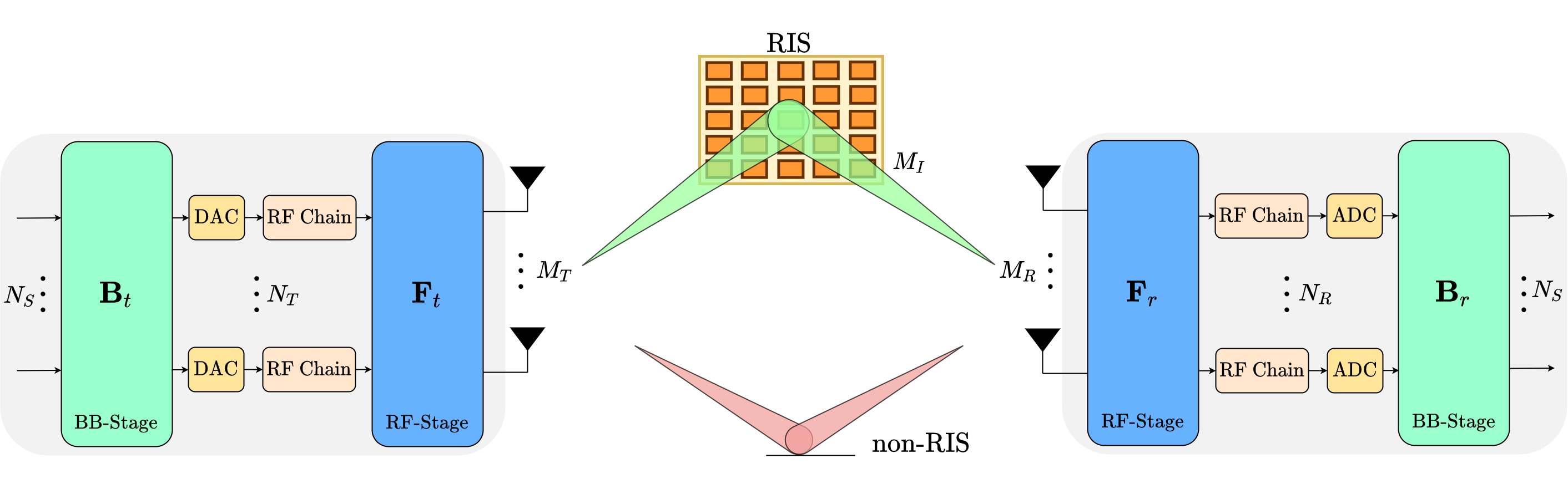
Figure 1: RIS-assisted hybrid mmWave massive MIMO system model.

In this work, we introduce an RIS-aided AB-HBF (RIS-AB-HBF) system requiring low CSI overhead for mmWave massive MIMO systems. By considering the 3D geometry-based mmWave channel model, a three-stage RIS-aided HBF system design is proposed: (i) RF beamformers, (ii) BB precoder/combiner, and (iii) RIS phase shift design. First, the transmit/receive RF beamformers are designed by using the slow time-varying angle-of-departure/angle-of-arrival (AoD/AoA) information of the channel, while the BB precoder and combiner are constructed exploiting the reduced-size effective channel seen from the BB-stage. Then, the RIS phase reflection matrix is designed via particle swarm optimization (PSO) to maximize the achievable rate of massive MIMO systems. Our comprehensive numerical results demonstrate that the RISs significantly enhance the achievable rate performance of the AB-HBF mmWave systems by alleviating the disruptive effects of the wireless propagation environment as well as reducing the CSI overhead.

II System Model

In this section, we present the system and channel models of the RIS-assisted HBF scheme for mmWave massive MIMO systems as well as provide their working principles.

II-A System Model and Problem Formulation

We consider an RIS-assisted hybrid mmWave massive MIMO architecture shown in Fig. 1, where there is a single RIS between the transmitter/receiver pair. As shown in Fig.1, the transmission is carried out via an RIS and non-RIS direct link between the transmitter (Tx) and the receiver (Rx). We assume that the Tx, Rx and RIS are in the form of uniform planar array (UPA). Here, the real-time controlled RIS is equipped with $M_{I}=M_{I_{x}}\times M_{I_{y}}$ dynamic reflecting elements that can be adjusted based on channel phases while the Tx and Rx are equipped with $M_{T}=M_{T_{x}}\times M_{T_{y}}$ and $M_{R}=M_{R_{x}}\times M_{R_{y}}$ antennas, respectively. The number of antennas along the $x$ and $y$-axis of the corresponding UPA are respectively denoted as $M_{i_{x}}$ and $M_{i_{y}}$ for $i\in\left\{I,T,R\right\}$. $N_{S}$ data streams are sent from the Tx via digital BB precoder (${\bf B}_{t}$) and analog RF beamformer (${\bf F}_{t}$), which are connected with $N_{T}$ RF chains. At the Rx, the received signal is combined via the analog RF beamformer (${\bf F}_{r}$) and digital BB combiner (${\bf B}_{r}$), which are connected with $N_{R}$ RF chains. Here we assume that the number of data streams is constraint as $N_{S}\leq\min\left(N_{T},N_{R}\right)$ and the number of RF chains are much smaller than both the number of transmit and receive antennas to exploit the benefit of HBF systems (i.e. $N_{T}\ll M_{T}$ and $N_{R}\ll M_{R}$).

The precoded signal ${\bf s}\in\mathbb{C}^{M_{T}}$ at the Tx is expressed as:

$${\bf s}={{\bf{F}}_{t}}{{\bf{B}}_{t}}{\bf{x}},$$ (1)

where ${\bf F}_{t}\in\mathbb{C}^{M_{T}\times N_{T}}$ represents the transmit RF beamformer, ${{\bf B}_{t}\in\mathbb{C}^{N_{T}\times N_{S}}}$ represents the BB precoder and ${\bf x}\in\mathbb{C}^{N_{S}}$ is the data symbol vector satisfying $\mathbb{E}\left\{{\bf x}{\bf x}^{H}\right\}={\bf I}_{N_{s}}$. The power constraint is also ensured for the transmitted power $P_{T}$ as $\mathbb{E}\big{\{}\big{\|}{\bf s}\big{\|}_{2}^{2}\big{\}}\leq P_{T}$.

The direct channel between the Tx and Rx is represented by ${\bf H}_{TR}\in\mathbb{C}^{M_{R}\times M_{T}}$, while the RIS-assisted link consists of two components: ${\bf H}_{TI}\in\mathbb{C}^{M_{I}\times M_{T}}$ is the channel from the Tx to RIS and ${\bf H}_{IR}\in\mathbb{C}^{M_{R}\times M_{I}}$ is the channel from the RIS to Rx. ${\bf\Theta}=\text{diag}{(e^{j\Omega_{1}},\dots,e^{j\Omega_{M_{I}}})}\in\mathbb{C}^{M_{I}\times M_{I}}$ is the matrix of RIS element response with $\Omega_{i}$ being the phase shift introduced by $i$th reflecting element of the RIS for $i=1,\dots,M_{I}$. At the receiver, the signal received from the RIS-assisted and direct link is obtained as:

$${\bf{y}}= {\bf{Hs}}+{\bf{v}}=({\bf H}_{IR}{\bf\Theta}{\bf H}_{TI}+{\bf H}_{TR})\bf{s}+{\bf{v}}$$ (2)

$$= {{({\bf H}_{IR}{\bf\Theta}{\bf H}_{TI}+{\bf H}_{TR})}}{{\bf{F}}_{t}}{{\bf{B}}_{t}}{\bf{x}}+{\bf{v}},$$

where ${\bf H}={\bf H}_{IR}{\bf\Theta}{\bf H}_{TI}+{\bf H}_{TR}\in\mathbb{C}^{M_{R}\times M_{T}}$ stands for the end-to-end channel matrix and ${{\bf{v}}\sim\mathcal{CN}\left({\bf 0},\sigma_{v}^{2}{\bf I}_{M_{R}}\right)}$ represents the additive white Gaussian noise. By using (1) and (2), the received signal after combining is written by:

$$\tilde{\bf y}={\bf B}_{r}\bm{\mathcal{H}}{\bf{B}}_{t}{\bf{x}}+{\bf B}_{r}{\bf F}_{r}{\bf{v}},$$ (3)

where $\bm{\mathcal{H}}={\bf F}_{r}{{({\bf H}_{IR}{\bf\Theta}{\bf H}_{TI}+{\bf H}_{TR})}}{{\bf{F}}_{t}}\in\mathbb{C}^{N_{r}\times N_{t}}$ is the effective channel matrix seen from the BB-stages, ${\bf F}_{r}\in\mathbb{C}^{N_{R}\times M_{T}}$ represents the receive RF beamformer, ${\bf B}_{r}\in\mathbb{C}^{N_{S}\times N_{R}}$ denotes the BB combiner.

In this work, our main aim is to efficiently design the transmit RF beamformer and BB precoder at the Tx (i.e., ${\bf F}_{t}$, ${\bf B}_{t}$), the receive RF beamformer and BB combiner at the Rx (i.e., ${\bf F}_{r}$, ${\bf B}_{r}$), and the phase shifts at the RIS (i.e. $\bf{\Theta}$) to maximize the achievable rate of the system as follows:

$$\max_{\left\{{\bf F}_{t},{\bf F}_{r},{\bf B}_{t},{\bf B}_{r},\bf{\Theta}\right\}} R= {\log_{2}}\left|{{{{\bf{I}}_{{N_{s}}}}+{\bf R}_{{w}}^{-1}}{\bf B}_{r}\bm{\mathcal{H}}{\bf B}_{t}{\bf B}_{t}^{H}\bm{\mathcal{H}}^{H}{\bf B}_{r}^{H}}\right|,$$ (4a)

s.t. $$~{}\bm{\mathcal{H}}={\bf F}_{r}{\bf HF}_{r}\in\mathbb{C}^{N_{r}\times N_{t}},$$ (4d)

$$\left|{\bf{F}}_{t}\left(m,n\right)\right|=\frac{1}{\sqrt{M_{t}}},\left|{\bf{F}}_{r}\left(m,n\right)\right|=\frac{1}{\sqrt{M_{r}}},~{}\forall\left(m,n\right),$$

$$\mathbb{E}\big{\{}{\big{\|}{\bf{x}}\big{\|}_{2}^{2}}\big{\}}={\rm{tr}}\left({{\bf{B}}_{t}^{H}{\bf{F}}_{t}^{H}{{\bf{F}}_{t}}{{\bf{B}}_{t}}}\right)\leq{P_{T}},$$

where ${\bf R}_{{w}}=\sigma_{v}^{2}{\bf B}_{r}{\bf F}_{r}{\bf F}_{r}^{H}{\bf B}_{r}^{H}$ is the covariance matrix of the noise ${\bf{w}}={\bf B}_{r}{\bf F}_{r}{\bf{v}}$. Since phase shifters are used in the implementation of RF beamformer, the constraint of the constant module is ensured as in (4d).

II-B Channel Model

In mmWave transmission, contrary to the conventional rich-scattering propagation environment, only a few spatial paths are experienced due to scattering limited propagation conditions. Hence, the mmWave channel will be sparse in the angular domain [16]. We assume that ${\bf H}_{l}$ ($l\in\left\{TR,TI,IR\right\}$) is a sum of the contributions of $C_{l}$ scattering clusters, each of which contribute $Z_{l,c}$ ($c=1,\dots,C_{l}$) propagation paths to the corresponding channel matrix. Each sub-channel is assumed to have $Z_{l}=\sum\nolimits_{c=1}^{C}Z_{l,c}$ paths in total between the terminals.

By following the UPA structure [10] and the 3D geometry-based mmWave channel model [17], the channel matrix between the terminals is defined as follows:

$${\bf H}_{l}= \sum\limits_{c=1}^{C_{l}}{\sum\limits_{p=1}^{Z_{l,c}}g_{c_{p}}^{l}}{{{\bm{\phi}}}_{l,r}}\left({{\gamma_{x,r}^{l,c_{p}}},{\gamma_{y,r}^{l,c_{p}}}}\right){\bm{\phi}}_{l,t}^{H}\big{(}{{\gamma_{x,t}^{l,c_{p}}},{\gamma_{y,t}^{l,c_{p}}}}\big{)}$$ (5)

$$= {{\bf{\Phi}}_{l}^{r}}{\bf G}_{l}{{\bf{\Phi}}_{l}^{t}},\>l\in\left\{TR,TI,IR\right\},$$

where $g_{c_{p}}^{l}\sim\mathcal{CN}\left(0,\frac{\beta^{l}}{P_{l}}\right)$ stands for the complex path gain of the $p^{th}$ path within the $c^{th}$ cluster of the corresponding channel with the path index of $c_{p}=p+\sum\nolimits_{u=1}^{c-1}Z_{l,u}$, and ${\bm{\phi}_{l,r}}\big{(}{\gamma_{x,r}^{l,c_{p}},\gamma_{y,r}^{l,c_{p}}}\big{)}$ is the receive phase response vector while the transmit phase response vector is denoted by ${\bm{\phi}_{l,t}}\big{(}{\gamma_{x,t}^{l,c_{p}},\gamma_{y,t}^{l,c_{p}}}\big{)}$. Here, $\beta^{l}$ represents the path loss of the corresponding path, which is inversely proportional to the terminal distances ($d_{l}$) as $\beta^{l}\propto d_{l}^{-\eta}$ with $\eta$ being path loss exponent for $l\in\left\{TR,TI,IR\right\}$. Moreover, ${\bf G}_{l}=\textrm{diag}\left(g_{1}^{l},\cdots,g_{P}^{l}\right)\in\mathbb{C}^{Z_{l}\times Z_{l}}$ represents the diagonal matrix including the complex path gains, ${{\bf{\Phi}}_{l}^{r}}$ and ${{\bf{\Phi}}_{l}^{t}}$ denote the receive and transmit phase response matrices for the corresponding channel, respectively.

Then, the transmit and receive phase response vectors are defined as:

$${\bm{\phi}_{ij,t}}\left({{\gamma_{x}^{l},\gamma_{y}^{l}}}\right) =\big{[}{1,{e^{j2\pi d{{\gamma_{x}^{l}}}}},\cdots,{e^{j2\pi d\left({{M_{i_{x}}}-1}\right){{\gamma_{x}^{l}}}}}}\big{]}^{T}\vspace{-1ex}$$ (6)

$$\otimes\big{[}{1,{e^{j2\pi d{{\gamma_{y}^{l}}}}},\cdots,{e^{j2\pi d\left({{M_{i_{y}}}-1}\right){{\gamma_{y}^{l}}}}}}\big{]}^{T},$$

$${\bm{\phi}_{ij,r}}\left({{\gamma_{x}^{l},\gamma_{y}^{l}}}\right) =\big{[}{1,{e^{j2\pi d{{\gamma_{x}^{l}}}}},\cdots,{e^{j2\pi d\left({{M_{j_{x}}}-1}\right){{\gamma_{x}^{l}}}}}}\big{]}^{T}$$ (7)

$$\otimes\big{[}{1,{e^{j2\pi d{{\gamma_{y}^{l}}}}},\cdots,{e^{j2\pi d\left({{M_{j_{y}}}-1}\right){{\gamma_{y}^{l}}}}}}\big{]}^{T},$$

where $(i,j)\in\left\{(T,R),(T,I),(I,R)\right\}$ and $d$ denotes the antenna spacing normalized by wavelength. From (5), (6) and (7), the slow time-varying transmit and receive phase response matrices for each sub-channel are respectively written by:

$${{\bf{\Phi}}_{l}^{t}}=\left[{\begin{array}[]{*{20}{c}}{{\bm{\phi}_{l,t}^{H}}\big{(}{{\gamma_{x,r}^{l,1}}},{{\gamma_{y,r}^{l,1}}}\big{)}}\\ {\vdots}\\ {{\bm{\phi}_{l,t}^{H}}\big{(}{{\gamma_{x,r}^{l,P_{l}}}},{{\gamma_{y,r}^{l,P_{l}}}}\big{)}}\end{array}}\right],~{}{{\bf{\Phi}}_{l}^{r}}=\left[{\begin{array}[]{*{20}{c}}{{\bm{\phi}_{l,r}^{H}}\big{(}{{\gamma_{x,r}^{l,1}}},{{\gamma_{y,r}^{l,1}}}\big{)}}\\ {\vdots}\\ {{\bm{\phi}_{l,r}^{H}}\big{(}{{\gamma_{x,r}^{l,P_{l}}}},{{\gamma_{y,r}^{l,P_{l}}}}\big{)}}\end{array}}\right]^{H}.$$ (8)

By considering the mean and spread parameters of AoA/AoD in Table I, at the arrival side of each sub-channel $l$ for $l\in\left\{TR,TI,IR\right\}$, the coefficients reflecting the elevation AoA and azimuth AoA of the $p^{th}$ path within the $c^{th}$ cluster are respectively defined as ${\gamma_{x,r}^{l,c_{p}}}=\sin\big{(}{{\theta_{r,c_{p}}^{l}}}\big{)}\cos\big{(}{{\psi_{r,c_{p}}^{l}}}\big{)}$ and ${\gamma_{y,r}^{l,c_{p}}}=\sin\big{(}{{\theta_{r,c_{p}}^{l}}}\big{)}\sin\big{(}{{\psi_{r,c_{p}}^{l}}}\big{)}$, where ${\theta_{r,c_{p}}^{l}}\in\big{[}{{\theta_{r,c}^{l}}-{\delta_{r,c}^{l,\theta}}},{{\theta_{r,c}^{l}}+{\delta_{r,c}^{l,\theta}}}\big{]}$ and ${\psi_{r,c_{p}}^{l}}\in\big{[}{{\psi_{r,c}^{l}}-{\delta_{r,c}^{l,\psi}}},{{\psi_{r,c}^{l}}+{\delta_{r,c}^{l,\psi}}}\big{]}$. At the departure side of each sub-channel $l$ for $l\in\left\{TR,TI,IR\right\}$, the elevation AoD and azimuth AoD of the $p^{th}$ path within the $c^{th}$ cluster are respectively defined as ${\gamma_{x,t}^{l,c_{p}}}=\sin\big{(}{{\theta_{t,c_{p}}^{l}}}\big{)}\cos\big{(}{{\psi_{t,c_{p}}^{l}}}\big{)}$ and ${\gamma_{y,t}^{l,c_{p}}}=\sin\big{(}{{\theta_{t,c_{p}}^{l}}}\big{)}\sin\big{(}{{\psi_{t,c_{p}}^{l}}}\big{)}$ , where ${\theta_{t,c_{p}}^{l}}\in\big{[}{{\theta_{t,c}^{l}}-{\delta_{t,c}^{l,\theta}}},{{\theta_{t,c}^{l}}+{\delta_{t,c}^{l,\theta}}}\big{]}$ and ${\psi_{t,c_{p}}^{l}}\in\big{[}{{\psi_{t,c}^{l}}-{\delta_{t,c}^{l,\psi}}},{{\psi_{t,c}^{l}}+{\delta_{t,c}^{l,\psi}}}\big{]}$.

TABLE I: AoA and AoD parameters of the $l^{\text{th}}$ channel for $l\in\left\{TR,TI,IR\right\}$.

$\theta_{r,c}^{l}$	Mean elevation AoA	$\theta_{t,c}^{l}$	Mean elevation AoD
$\delta_{r,c}^{l,\theta}$	Elevation AoA spread	$\delta_{t,c}^{l,\theta}$	Elevation AoD spread
$\psi_{r,c}^{l}$	Mean azimuth AoA	$\psi_{t,c}^{l}$	Mean azimuth AoD
$\delta_{r,c}^{l,\psi}$	Azimuth AoA spread	$\delta_{t,c}^{l,\psi}$	Azimuth AoD spread

III RIS-Aided Angular-Based Hybrid Beamforming

In this section, we respectively provide the design of RF beamformers, BB precoder/combiner and phase shift matrix of the RIS for the proposed RIS-aided AB-HBF system. Our primary goal is to maximize the achievable rate of the system as well as reduce the CSI overhead size and the hardware complexity. From this point of view, first, the design procedures of RF beamformers is introduced based on slow-time varying angular parameters. Afterwards, BB precoder/combiner is designed by the singular value decomposition (SVD) and water filling algorithm using effective channel with reduced size. Finally, the phase shifts of the RIS, which enhances the system capacity, is obtained by applying the PSO method.

III-A RF Beamformers

In order to design RF-stage efficiently, the range of the azimuth and elevation AoA/AoD angles of the existing paths in the clusters is first required to be appropriately defined as in [11]. Therefore, AoA and AoD angle supports are respectively defined based on (5) as:

$${\Upsilon_{\textrm{AoA}}} = \Big{\{}{{{\left[{{\gamma_{x}},{\gamma_{y}}}\right]}}={{\left[\sin\left(\theta\right){\cos\left(\psi\right),\sin\left(\theta\right)\sin\left(\psi\right)}\right]}}}\hskip 0.86108pt\Big{|}\hskip 0.86108pt\theta\in{\bm{\theta}}_{r},\psi\in{\bm{\psi}}_{r}\Big{\}},\vspace{-0.6ex}\vspace{0.5ex}$$ (9a)

$$\Upsilon_{\textrm{AoD}} = \Big{\{}{{{\left[{{\gamma_{x}},{\gamma_{y}}}\right]}}={{\left[\sin\left(\theta\right){\cos\left(\psi\right),\sin\left(\theta\right)\sin\left(\psi\right)}\right]}}}\hskip 0.86108pt\Big{|}\hskip 0.86108pt\theta\in{\bm{\theta}}_{t},\psi\in{\bm{\psi}}_{t}\Big{\}},\vspace{-0.6ex}$$ (9b)

where ${\bm{\theta}}_{r}={\bm{\theta}}_{r}^{TI}\cup{\bm{\theta}}_{r}^{TR}$, ${\bm{\psi}}_{r}={\bm{\psi}}_{r}^{TI}\cup{\bm{\psi}}_{r}^{TR}$, ${\bm{\theta}}_{t}={\bm{\theta}}_{t}^{IR}\cup{\bm{\theta}}_{t}^{TR}$, and ${\bm{\psi}}_{t}={\bm{\psi}}_{t}^{IR}\cup{\bm{\psi}}_{t}^{TR}$. Here, the elevation and azimuth AoA supports for the corresponding sub-channels are respectively defined as: ${\bm{\theta}}_{r}^{l}=\cup_{c=1}^{C_{l}}\big{[}{{\theta_{r,c}^{l}}-{\delta_{r,c}^{l,\theta}}},{{\theta_{r,c}^{l}}+{\delta_{r,c}^{l,\theta}}}\big{]}$ and ${\bm{\psi}}_{r}^{l}=\cup_{c=1}^{C_{l}}\big{[}{{\psi_{r,c}^{l}}-{\delta_{r,c}^{l,\psi}}},{{\psi_{r,c}^{l}}+{\delta_{r,c}^{l,\psi}}}\big{]}$ for $l\in\left\{IR,TR\right\}$. Then, the elevation and azimuth AoD supports for the corresponding sub-channels are respectively obtained as: ${\bm{\theta}}_{t}^{l}=\cup_{c=1}^{C_{l}}\big{[}{{\theta_{t,c}^{l}}-{\delta_{t,c}^{l,\theta}}},{{\theta_{t,c}^{l}}+{\delta_{t,c}^{l,\theta}}}\big{]}$ and ${\bm{\psi}}_{t}^{l}=\cup_{c=1}^{C_{l}}\big{[}{{\psi_{t,c}^{l}}-{\delta_{t,c}^{l,\psi}}},{{\psi_{t,c}^{l}}+{\delta_{t,c}^{l,\psi}}}\big{]}$ for $l\in\left\{TI,TR\right\}$.

By using (2) and (5), the effective channel seen from the BB-stages can be reorganized as:

$$\bm{\mathcal{H}}= {\bf F}_{r}{\bf H}{\bf F}_{t},$$ (10)

$$= {\bf F}_{r}({{\bf{\Phi}}_{IR}^{r}}{\bf G}_{IR}{{\bf{\Phi}}_{IR}^{t}}{\bf\Theta}{{\bf{\Phi}}_{{TI}}^{r}}{\bf G}_{TI}{{\bf{\Phi}}_{TI}^{t}}$$

$$+{{\bf{\Phi}}_{{TR}}^{r}}{\bf G}_{TR}{{\bf{\Phi}}_{TR}^{t}}){\bf F}_{t}.$$

In order to optimize the receive (transmit) beamforming gain and take advantage of all degrees of freedom enabled by the channel, the subspace spanned by ${{\bf{\Phi}}_{IR}^{r}}$ and ${{\bf{\Phi}}_{TR}^{r}}$ (${{\bf{\Phi}}_{TI}^{t}}$ and ${{\bf{\Phi}}_{TR}^{t}}$) should be encompassed in the columns of ${\bf F}_{r}$ (${\bf F}_{t}$): $\textrm{Span}\left({\bf F}_{r}\right)\subset\left(\textrm{Span}\left({{\bf{\Phi}}_{IR}^{r}}\right)\cup\textrm{Span}\left({{\bf{\Phi}}_{TR}^{r}}\right)\right)$ and $\textrm{Span}\left({\bf F}_{t}\right)\subset\left(\textrm{Span}\left({{\bf{\Phi}}_{TI}^{t}}\right)\cup\textrm{Span}\left({{\bf{\Phi}}_{TR}^{t}}\right)\right)$ should be satisfied. Afterwards, the columns of the RF precoder matrix are created using the transmit steering vector ${{\bf{a}}_{t}}\left({{\gamma_{x}},{\gamma_{y}}}\right)=\frac{1}{{\sqrt{{M_{t}}}}}{\big{[}{1,{e^{j2\pi d\gamma_{x}}},\cdots,{e^{j2\pi d\left({{M_{T_{x}}}-1}\right)\gamma_{x}}}}\big{]}^{T}}\otimes{\big{[}{1,{e^{j2\pi d\gamma_{y}}},\cdots,{e^{j2\pi d\left({{M_{T_{y}}}-1}\right)\gamma_{y}}}}\big{]}^{T}}\in\mathbb{C}^{M_{T}}$. The quantized angle pairs are defined as follows to obtain $M_{T}$ orthogonal transmit steering vectors as the minimum number of angle pairs spanning the entire elevation and azimuth space [10, 11]: ${{\kappa_{x,t}^{m}}=\frac{2m-1}{{{M_{T_{x}}}}}}-1$ for $m=1,\cdots,{M_{T_{x}}}$ and ${{\kappa_{y,t}^{n}}=\frac{2n-1}{{{M_{T_{y}}}}}}-1$ for $n=1,\cdots,{M_{T_{y}}}$. Thus, while minimizing the use of the RF chain by covering the entire AoD support, the quantized angle pairs within the AoD support are written as:

$$\left({\kappa_{x,t}^{m},\kappa_{y,t}^{n}}\right)~{}\Big{|}\Big{.}~{}{\gamma_{x}}\in{\bm{\kappa}}_{x,t}^{m},{\gamma_{y}}\in{\bm{\kappa}}_{y,t}^{n},\left({{\gamma_{x}},{\gamma_{y}}}\right)\in\Upsilon_{\textrm{AoD}},\vspace{-1ex}$$ (11)

where ${\bm{\kappa}}_{x,t}^{m}=\big{[}{\kappa_{x,t}^{m}-\frac{1}{{{M_{T_{x}}}}},\kappa_{x,t}^{m}+\frac{1}{{{M_{T_{x}}}}}}\big{]}$ and ${\bm{\kappa}}_{y,t}^{n}=\big{[}{\kappa_{y,t}^{n}-\frac{1}{{{M_{T_{y}}}}},\kappa_{y,t}^{n}+\frac{1}{{{M_{T_{y}}}}}}\big{]}$ respectively represent the boundary of $\kappa_{x,t}^{m}$ and $\kappa_{y,t}^{n}$. Therefore, the RF precoder with $N_{T}$ quantized angle-pairs is constructed based on (9b) as:

$${{\bf{F}}_{t}}=\big{[}{{\bf{a}}_{t}\big{(}{\kappa^{m_{1}}_{x,t},\kappa^{n_{1}}_{y,t}}\big{)},\cdots,{\bf{a}}_{t}\big{(}{\kappa^{m_{N_{T}}}_{x,t},\kappa^{n_{N_{T}}}_{y,t}}\big{)}}\big{]}\in\mathbb{C}^{M_{T}\times N_{T}}.\vspace{-1ex}$$ (12)

Following the similar procedure for the RF combiner ($\bf{F}_{r}$), the receive steering vector is obtained as: ${{\bf{a}}_{r}}\left({{\gamma_{x}},{\gamma_{y}}}\right)=\frac{1}{{\sqrt{{M_{R}}}}}{\big{[}{1,{e^{j2\pi d\gamma_{x}}},\cdots,{e^{j2\pi d\left({{M_{R_{x}}}-1}\right)\gamma_{x}}}}\big{]}^{T}}\otimes{\big{[}{1,{e^{j2\pi d\gamma_{y}}},\cdots,{e^{j2\pi d\left({{M_{R_{y}}}-1}\right)\gamma_{y}}}}\big{]}^{T}}\in\mathbb{C}^{M_{R}}$. The quantized angle pairs are given by ${{\kappa_{x,r}^{m}}=\frac{2m-1}{{{M_{R_{x}}}}}}-1$ for $m=1,\cdots,{M_{R_{x}}}$ and ${{\kappa_{y,r}^{n}}=\frac{2n-1}{{{M_{R_{y}}}}}}-1$ for $n=1,\cdots,{M_{R_{y}}}$.

In order to minimize the use of the RF chain in the receiver side by covering the entire AoA support, the quantized angle pairs within the AoA support are obtained as:

$$\left({\kappa_{x,r}^{m},\kappa_{y,r}^{n}}\right)~{}\Big{|}\Big{.}~{}{\gamma_{x}}\in{\bm{\kappa}}_{x,r}^{m},{\gamma_{y}}\in{\bm{\kappa}}_{y,r}^{n},\left({{\gamma_{x}},{\gamma_{y}}}\right)\in\Upsilon_{\textrm{AoA}},\vspace{-1ex}$$ (13)

where ${\bm{\kappa}}_{x,t}^{m}=\big{[}{\kappa_{x,t}^{m}-\frac{1}{{{M_{T_{x}}}}},\kappa_{x,t}^{m}+\frac{1}{{{M_{T_{x}}}}}}\big{]}$ and ${\bm{\kappa}}_{y,r}^{n}=\big{[}{\kappa_{y,r}^{n}-\frac{1}{{{M_{R_{y}}}}},\kappa_{y,r}^{n}+\frac{1}{{{M_{R_{y}}}}}}\big{]}$ respectively denote the boundary of $\kappa_{x,r}^{m}$ and $\kappa_{y,r}^{n}$. Finally, the RF combiner with $N_{R}$ quantized angle-pairs is constructed fulfilling AoA support in (9a) as:

$${{\bf{F}}_{r}}=\big{[}{{\bf{a}}_{r}\big{(}{\kappa^{m_{1}}_{x,r},\kappa^{n_{1}}_{y,r}}\big{)},\cdots,{\bf{a}}_{r}\big{(}{\kappa^{m_{N_{R}}}_{x,r},\kappa^{n_{N_{R}}}_{y,r}}\big{)}}\big{]}\in\mathbb{C}^{M_{R}\times N_{R}}.\vspace{-0.5ex}$$ (14)

It should be noted that the unitary property for RF beamformers (i.e. ${\bf F}_{t}^{H}{\bf F}_{t}={\bf I}_{N_{T}}$, ${\bf F}_{r}{\bf F}_{r}^{H}={\bf I}_{N_{R}}$) and the constant modulus condition provided in (4d) are satisfied in the RF beamformer design stage.

III-B Baseband Precoder/Combiner

After the design of the RF beamformers, this subsection focuses on the BB precoder/combiner design using the low-dimensional effective channel matrix given in (10). The singular value decomposition (SVD) of effective channel matrix$\bm{\mathcal{H}}$ is obtained as $\bm{\mathcal{H}}={\bf U\Sigma V}^{H}$, where ${\bf U}\in\mathbb{C}^{N_{R}\times\textrm{rank}\left(\bm{\mathcal{H}}\right)}$ represents a tall unitary matrix, ${\bf\Sigma}=\textrm{diag}\big{(}\sigma_{1}^{2},\cdots,\sigma_{\textrm{rank}\left(\bm{\mathcal{H}}\right)}^{2}\big{)}\in\mathbb{R}^{\textrm{rank}\left(\bm{\mathcal{H}}\right)\times\textrm{rank}\left(\bm{\mathcal{H}}\right)}$ denotes a diagonal matrix of the singular values in the descending order and ${\bf V}\in\mathbb{C}^{N_{T}\times\textrm{rank}\left(\bm{\mathcal{H}}\right)}$ stands for a tall unitary matrix. Here, ${\bf V}$ can be partitioned as ${\bf V}=\left[{\bf V}_{1},{\bf V}_{2}\right]$ for ${\bf V}_{1}\in\mathbb{C}^{N_{T}\times N_{S}}$ under $\textrm{rank}\left(\bm{\mathcal{H}}\right)\geq N_{S}$.

Similar to [18, 11], the optimal solution for the BB precoder can be represented as:

$${\bf B}_{t}={\bf V}_{1}{\bf\Gamma}^{\frac{1}{2}}\in\mathbb{C}^{N_{T}\times N_{T}},$$ (15)

where ${\bf\Gamma}=\textrm{diag}\left(\Gamma_{1},\cdots,\Gamma_{N_{S}}\right)\in\mathbb{R}^{N_{S}\times N_{S}}$ represents a transmit power matrix with $\sum\nolimits_{n=1}^{N_{S}}\Gamma_{n}={P_{T}}$ for meeting the power constraint given in (4d). By using the water filling power control solution [19], the powers are allocated as:

$${\Gamma_{n}}={\left({\mu-\frac{\sigma_{v}^{2}}{{P_{T}\sigma_{n}^{2}}}}\right)^{+}},{\textrm{ s.t.}}\sum\limits_{n=1}^{N_{S}}{\left({\mu-\frac{\sigma_{v}^{2}}{{P_{T}\sigma_{n}^{2}}}}\right)^{+}}=P_{T}.\vspace{-1ex}$$ (16)

Then, considering the given RF beamformer (${\bf F}_{t}$/${\bf F}_{r}$), phase response matrix (${\bf\Theta}$) and BB precoder (${\bf B}_{t}$), we strive to design the BB combiner (${\bf B}_{r}$) that minimize the mean-squared-error (MSE) between the transmitted and processed received signals. Based on (3), the MSE expression can therefore be stated as:

$${\bf{e}_{\rm{MSE}}}= \mathbb{E}\big{\{}{{{\big{\|}{\tilde{\bf{y}}-{\bf{x}}}\big{\|}}^{2}}}\big{\}}={\rm{tr}}\big{(}\mathbb{E}{\big{\{}{\tilde{\bf{y}}{{\tilde{\bf{y}}}^{H}}-{\bf{x}}{{\tilde{\bf{y}}}^{H}}-\tilde{\bf{y}}{{\bf{x}}^{H}}+{\bf{x}}{{\bf{x}}^{H}}}\big{\}}}\big{)}$$ (17)

$$= \rm{tr}\Big{(}{{\bf B}_{r}\bm{\mathcal{H}}{{\bf{B}}_{t}}{{\bf{B}}_{t}^{H}}\bm{\mathcal{H}}^{H}}{\bf B}_{r}^{H}+{\bf B}_{r}{\bf R}_{{q_{r}}}{\bf B}_{r}^{H}$$

$$-{{{\bf{B}}_{t}^{H}}\bm{\mathcal{H}}^{H}{\bf B}_{r}^{H}}+{\bf I}_{N_{s}}\Big{.}\Big{)}.$$

For the purpose of finding the optimal solution for (17), the differentiation rules for the complex-valid matrices are applied. Then, the derivative of $\bf{e}_{\textrm{MSE}}$ with respect to BB combiner (${\bf B}_{r}$) is calculated as:

$$\frac{{\partial\bf{e}_{{\rm{MS}}{{\rm{E}}{}}}}}{{\partial{{\bf{B}}_{r}}}} =2{\bf B}_{r}{\bm{\mathcal{H}}{{\bf{B}}_{t}}{{\bf{B}}_{t}^{H}}\bm{\mathcal{H}}^{H}}-2{{{\bf{B}}_{t}^{H}}\bm{\mathcal{H}}^{H}}.$$ (18)

Finally, the BB combiner meeting the minimum MSE criterion in (17) can be obtained as follows:

$${\bf{B}}_{r}={\bf{B}}_{t}^{H}\bm{\mathcal{H}}^{H}\left(\bm{\mathcal{H}}{{\bf{B}}_{t}}{{\bf{B}}_{t}^{H}}\bm{\mathcal{H}}^{H}\right)^{-1}.\vspace{-1ex}$$ (19)

III-C RIS Phase Shift Design

In this subsection, phase shifts of the RIS elements are adjusted by optimizing the achievable rate of the system via the PSO algorithm. In PSO, each particle reconfigures its position at every step by moving through multidimensional space with its own experience and the experience of its peers towards an optimum solution by the whole swarm [20]. Under given RF beamformers (${\bf F}_{t},{\bf F}_{r}$) and BB precoder/combiner (${\bf B}_{t}$, ${\bf B}_{r}$), the optimization problem for maximizing the achievable rate can be formulated as:

$$\max_{\left\{\bf{\Theta}\right\}}{} R\left({\bf F}_{t},{\bf F}_{r},{\bf B}_{t},{\bf B}_{r},\bf{\Theta}\right)$$ (20)

s.t. $${\bf\Theta}=\text{diag}{(e^{j\Omega_{1}},\dots,e^{j\Omega_{M_{I}}})}$$

$$\mathbb{E}\big{\{}{\big{\|}{\bf{x}}\big{\|}_{2}^{2}}\big{\}}={\rm{tr}}\left({{\bf{B}}_{t}^{H}{\bf{F}}_{t}^{H}{{\bf{F}}_{t}}{{\bf{B}}_{t}}}\right)\leq{P_{T}}$$

$$\Omega_{i}\in[0,2\pi],\forall i,\vspace{-1ex}$$

where $R\left({\bf F}_{t},{\bf F}_{r},{\bf B}_{t},{\bf B}_{r},\bf{\Theta}\right)$ is given in (4a). In our PSO solution, the phase shifts of the RIS elements ($\Omega_{i}$, $i\in{1,\dots,M_{I}}$) are modeled as the positions of the particles, and the objective function in (20) is considered as the fitness function of PSO.

$N_{\textrm{par}}$ particles are randomly initialized with position ${\bf p}\in\mathbb{C}^{M_{I}}$ and velocity ${\bf v}\in\mathbb{C}^{M_{I}}$. Each particle has a memory for its local best position (${\bf p}_{\textrm{best},i}^{(q)}$) and the global best position (${\bf p}_{G}^{(q)}$), where the superiority of a position is evaluated by the given fitness function. Here, ${\bf p}_{\textrm{best},i}^{(q)}$ is the best position that the $i^{\textrm{th}}$ particle has achieved while ${\bf p}_{G}^{\textrm{(t)}}$ is the best position achieved by any of the particles in the entire swarm in the $q^{\textrm{th}}$ iteration. For each iteration, the velocity and position of each particle are updated according to:

$${\bf v}_{i}^{(q+1)}= \zeta{\bf v}_{i}^{(q)}+u_{1}\rho_{1}\big{(}{\bf p}_{\textrm{best},i}^{(q)}-{\bf p}_{i}^{(q)}\big{)}+u_{2}\rho_{2}\big{(}{\bf p}_{G}^{(q)}-{\bf p}_{i}^{(q)}\big{)},$$ (21)

$${\bf p}_{i}^{(q+1)}= {\bf v}_{i}^{(q+1)}+{\bf p}_{i}^{(q)},$$

where $\zeta$ is the inertia weight of velocity, $\rho_{1}$ and $\rho_{2}$ are the acceleration constants, and $u_{1}$ and $u_{2}$ are uniformly distributed random numbers in $[0,1]$. Through the iterations, the particles move from ${\bf p}_{i}^{(q)}$ to ${\bf p}_{i}^{(q+1)}$. Finally, after $Q$ iterations, the RIS phase shift matrix is determined at the last iteration as ${\bf\Theta}=\textrm{diag}\big{(}\exp\big{(}{j{\bf p}_{G}^{(Q)}}\big{)}\big{)}$. The summary of the proposed RIS-aided AB-HBF system design including three stages is precisely explained in Algorithm 1.

Algorithm 1 Proposed RIS-aided AB-HBF System Design

0:  $\bm{\mathcal{H}}$, $\Upsilon_{\textrm{AoA}}$, $\Upsilon_{\textrm{AoD}}$, $P_{T}$, $Q$, $N_{\textrm{par}}$, $\zeta$, $\rho_{1}$, $\rho_{2}$

0:  ${\bf F}_{t}$, ${\bf F}_{r}$, ${\bf B}_{t}$, ${\bf B}_{r}$, ${\bf\Theta}$

  Build ${\bf F}_{t}$ and ${\bf F}_{r}$ via (12) and (14), respectively.

  for $q=1:Q$ do

     Calculate each particle’s velocity ${\bf v}_{i}^{(q)}$ via (21).

     Calculate each particle’s position ${\bf p}_{i}^{(q)}$ via (21).

     Find each particle’s achievable rate via (20).

     Update personal best ${\bf p}_{\textrm{best},i}^{(q)}$ and global best ${\bf p}_{{G}}^{(q)}$.

  end for

  Set RIS phase-shift matrix as ${\bf\Theta}=\textrm{diag}\big{(}\exp\big{(}{j{\bf p}_{G}^{(Q)}}\big{)}\big{)}$.

  Build ${\bf B}_{t}$ and ${\bf B}_{r}$ via (15) and (19), respectively.

IV Numerical Results

In this section, we provide comprehensive numerical results to investigate the performance of the proposed RIS-aided AB-HBF system. Here, Table II presents the common parameters for all simulations considering the geometry-based mmWave channel given in (5). Due to the simplicity, we assume that all subchannels have $Z_{l,c}=5$ paths within a single cluster $C_{l}=1$ for $l\in\left\{TR,TI,IR\right\}$ and $c=1$. Moreover, the azimuth and elevation AoA/AoD spreads for all subchannels are assumed to be the same as $\delta_{i,c}^{l,j}=$$$ for $l\in\left\{TR,TI,IR\right\}$, $i=\in\left\{t,r\right\}$, $j\in\left\{\theta,\psi\right\}$ and $c=1$. The spacing between two antennas/reflectors is also $d=0.5$ due to the half-wavelength separation. The top view of the simulation setup, including the terminal distances, is also illustrated in Fig. 2. Here, the Tx-Rx channel is assumed to be nearly blocked under non-line-of-sight (NLOS) conditions, while the RIS-assisted cascade channel is assumed to have LOS conditions.

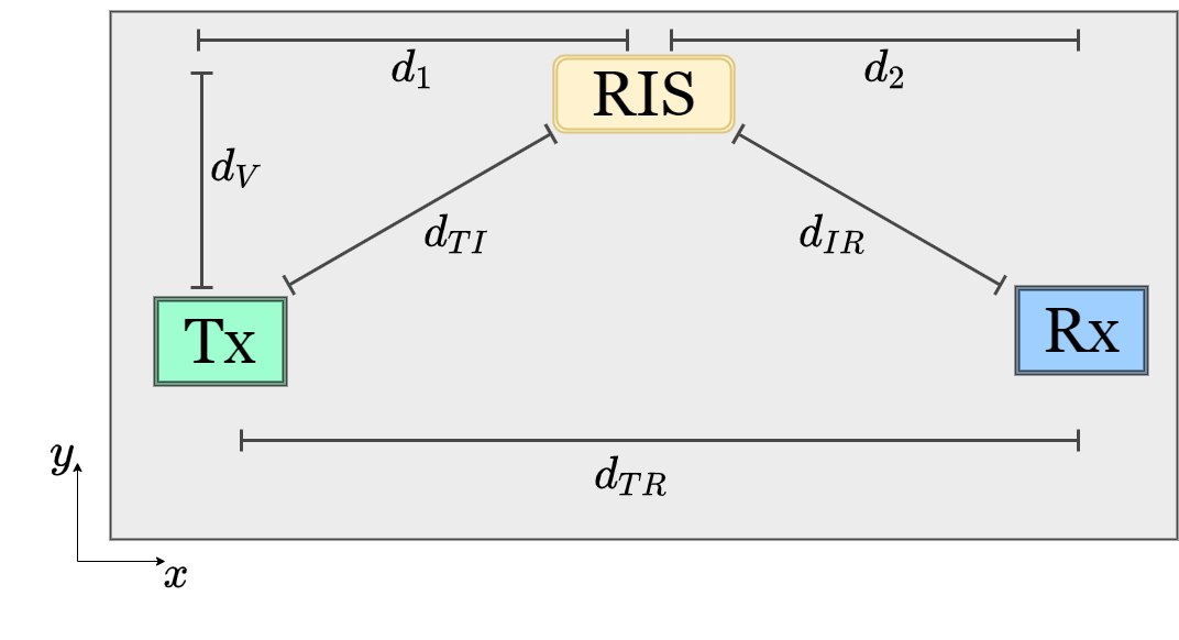
Figure 2: Top view of simulation setup for the proposed RIS-aided hybrid MIMO system.

TABLE II: Simulation parameters.

# of transmit antennas	$M_{T}=8\times 8=64$
# of receive antennas	$M_{R}=4\times 4=16$
# of RIS elements	$M_{I}=16\times 16=256$
# of RF Chains	$N_{T}=6$, $N_{R}=2$
# of data streams	$N_{S}=2$
# of clusters for ${\bf H}_{l}$	$C_{l}=1$ for $l\in\left\{TR,TI,IR\right\}$
# of paths for ${\bf H}_{l}$	$Z_{l,c}=5$ for $l\in\left\{TR,TI,IR\right\}$
Noise PSD	$-174$ dBm/Hz
Channel Bandwidth	$10$ kHz
PSO # of iterations	$T=200$
PSO # of particles	$N_{\textrm{par}}=100$
Path loss exponent	$\eta=2.3$ for LOS, $\eta=4.5$ for NLOS [21]
Mean elevation AoA/AoD	$\theta_{i,c}^{TR}=$$$ , $\theta_{i,c}^{TI}=$$$, $\theta_{i,c}^{IR}=$$$, $i\in\left\{t,r\right\}$
Mean azimuth AoA/AoD	$\phi_{i,c}^{TR}=$$$ , $\phi_{i,c}^{TI}=$$$ , $\phi_{i,c}^{IR}=$$$, $i\in\left\{t,r\right\}$

Fig. 3(a) compares the achievable rate performance for the AB-HBF system with or without RIS for varying Tx-RIS separation under fixed Tx and Rx positions. In this comparison, the RIS-assisted AB-HBF schemes with random and constant phase adjustment are also considered as a benchmark system for $d_{TR}=200$ and $d_{V}=5$ m. In this scenario, it is observed that RIS significantly improves system performance when the direct link between the Tx and Rx is nearly blocked. For $d_{1}=100$ m, the PSO-based RIS-assisted AB-HBF system provides $25$ dB superiority to the conventional AB-HBF system, while $4.5$ dB superiority to the random phase-adjusted RIS-AB-HBF system. Fig. 3(a) also provides practical perspective for the effective positioning of the RIS. For $d_{1}=20$ m, the achievable rate will be measured as $10.47$ bps/Hz, while it will approximately reduce to one-third, measuring $3.24$ bps/Hz for $d_{1}=100$ m. In Fig. 3(b), the achievable rate performance of the AB-HBF system is illustrated depending on the position of Rx changing along the $x$-axis under the fixed Tx and RIS positions. Here, the fixed distances between the Tx and RIS are given as $d_{1}=10$ m and $d_{V}=20$ m. However, doubling the $d_{TR}$ ($25$ m to $50$ m) will result in a performance loss of $22.85\%$ in the PSO-based RIS-AB-HBF system, $28.2\%$ in the random phase RIS AB-HBF, $57.03\%$ in the constant phase RIS-AB-HBF, and $76.53\%$ in the conventional AB-HBF. From the presented results in Fig. 3, we conclude that the presence of an RIS in AB-HBF systems alleviates the deteriorated channel conditions by providing an additional reliable transmission link alternative to the blocked Tx-Rx link. Thus, a remarkable increase in achievable rate performance is achieved by effectively positioning the RIS even in the absence of a LOS Tx-Rx channel.

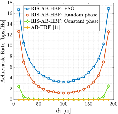
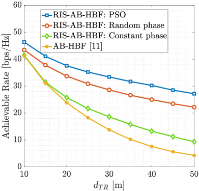
Figure 3: Comparison of achievable rate performance for AB-HBF system with or without RIS for varying (a) $d_{1}$ and (b) $d_{TR}$.

In Fig. 4, we present achievable rate comparison results for PSO-based, random and constant phase adjustment for the RIS-aided AB-HBF system at $100$ and $400$ m $d_{TR}$ values with increasing $P_{T}$. Here, the distances for this setup are assumed as $d_{V}=5$ and $d_{2}=4d_{1}$. Fig. 4 gives an useful insights for the different operating modes of an RIS. Even if the phase shifts of the RIS are set to a fixed value, a notable increase in the system performance can be achieved by providing an additional LOS path for the transmission. However, when the received signal quality is below a certain threshold value, the transmission performance can be increased by activating the PSO-assisted phase adjustment algorithm. From this point of view, the use of RISs in AB-HBF systems may has the potential to provide more promising advantages in terms of reliability and flexibility in system design.

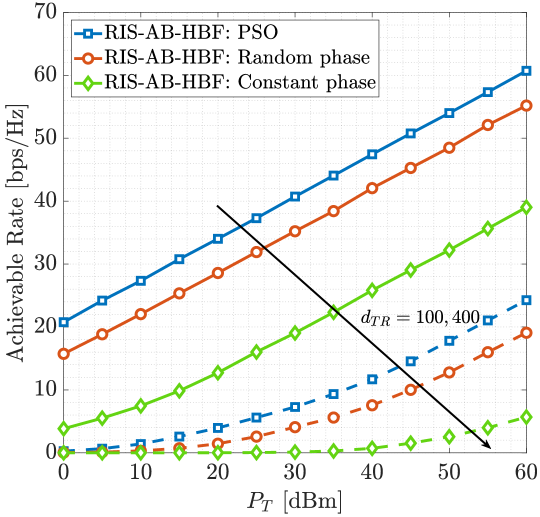
Figure 4: Achievable rate comparison of different phase adjustment methods in RIS-aided AB-HPC systems for varying $M_{I}$.

Finally, Fig. 5 demonstrates the achievable rate comparison of the AB-HPC system in the presence of an RIS under varying $M_{I}$ for $d_{TR}=100$, $d_{1}=10$, $d_{2}=80$ and $d_{V}=10$ m. As observed from Fig. 5, increasing $M_{I}$ significantly enhance the effect of the RIS in transmission both in the case of PSO-based and random phase adjustment. While the constant phase adjustment contributes to the transmission by providing a reliable LOS path, it will become saturated at increasing $M_{I}$ values. Although the random phase adjustment also leads to an remarkable increase in the system performance, the effect of increasing $M_{I}$ is more evident for the PSO-based RIS-AB-HBF system. For instance, the PSO-based scenario provides a $3$ dB advantage over the random phase adjustment case for $M_{I}=10$, while provides $4.5$ dB increase for $M_{I}=100$.

V Conclusions

In this paper, a RIS-aided AB-HBF system has been introduced for the hybrid mmWave massive MIMO system. In this context, we have investigated a number of RIS-aided AB-HBF systems in terms of achievable rate performance to find the most efficient architecture where the RIS and HBF technologies work in harmony with each other. It has been shown via extensive numerical results that a remarkable increase in achievable rate performance is achieved by effectively positioning the RIS even in the absence of a LOS channel between the Tx and Rx. The use of RISs in the AB-HBF systems may have the potential to provide more favorable advantages in terms of reliability and flexibility in system design.

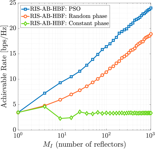
Figure 5: Achievable rate performance of the AB-HBF system with and without RIS for varying $M_{I}$.

References

• [1] W. Jiang et al., “The road towards 6G: A comprehensive survey,” IEEE Open J. Commun. Society, vol. 2, pp. 334–366, 2021.
• [2] E. G. Larsson et al., “Massive MIMO for next generation wireless systems,” IEEE Commun. Mag., vol. 52, no. 2, pp. 186–195, Feb. 2014.
• [3] E. Basar et al., “Reconfigurable intelligent surfaces for future wireless networks: A channel modeling perspective,” IEEE Wireless Commun., vol. 28, no. 3, pp. 108–114, 2021.
• [4] E. Basar et al., “Wireless communications through reconfigurable intelligent surfaces,” IEEE Access, pp. 116 753–116 773, Sep. 2019.
• [5] C. Huang et al., “Reconfigurable intelligent surfaces for energy efficiency in wireless communication,” IEEE Trans. Wireless Commun., Aug. 2019.
• [6] I. Yildirim et al., “Modeling and analysis of reconfigurable intelligent surfaces for indoor and outdoor applications in future wireless networks,” IEEE Trans. Commun., vol. 69, no. 2, pp. 1290–1301, 2021.
• [7] I. Yildirim et al., “Hybrid RIS-empowered reflection and decode-and-forward relaying for coverage extension,” IEEE Commun. Lett., vol. 25, no. 5, pp. 1692–1696, 2021.
• [8] N. Fatema et al., “Massive MIMO linear precoding: A survey,” IEEE Syst. J., vol. 12, no. 4, pp. 3920–3931, Dec. 2017.
• [9] I. Ahmed et al., “A survey on hybrid beamforming techniques in 5G: Architecture and system model perspectives,” IEEE Commun. Surveys Tuts., vol. 20, no. 4, pp. 3060–3097, 4th Quart. 2018.
• [10] A. Koc et al., “3D angular-based hybrid precoding and user grouping for uniform rectangular arrays in massive MU-MIMO systems,” IEEE Access, vol. 8, pp. 84 689–84 712, May 2020.
• [11] A. Koc et al., “Hybrid millimeter-wave massive MIMO systems with low CSI overhead and few-bit DACs/ADCs,” in 2020 IEEE 92nd Veh. Technol. Conf. (VTC2020-Fall), Dec. 2020, pp. 1–5.
• [12] A. Koc et al., “Swarm intelligence based power allocation in hybrid massive MIMO systems,” in 2021 IEEE Wireless Commun. and Netw. Conf. (WCNC), Mar. 2021, pp. 1–7.
• [13] P. Wang et al., “Joint transceiver and large intelligent surface design for massive MIMO mmWave systems,” IEEE Trans. Wireless Commun., vol. 20, no. 2, pp. 1052–1064, 2021.
• [14] K. Ying et al., “GMD-based hybrid beamforming for large reconfigurable intelligent surface assisted millimeter-wave massive MIMO,” IEEE Access, vol. 8, pp. 19 530–19 539, 2020.
• [15] S. H. Hong et al., “Hybrid beamforming for intelligent reflecting surface aided millimeter wave MIMO systems,” IEEE Trans. Wireless Commun (Early Access), 2022.
• [16] A. Alkhateeb et al., “MIMO precoding and combining solutions for millimeter-Wave systems,” IEEE Commun. Mag., vol. 52, no. 12, pp. 122–131, Dec. 2014.
• [17] X. Cheng et al., “Communicating in the real world: 3D MIMO,” IEEE Wireless Commun., vol. 21, no. 4, pp. 136–144, Aug. 2014.
• [18] S. Park et al., “Dynamic subarrays for hybrid precoding in wideband mmWave MIMO systems,” IEEE Trans. Wireless Commun., vol. 16, no. 5, pp. 2907–2920, Mar. 2017.
• [19] F. Sohrabi et al., “Hybrid analog and digital beamforming for mmWave OFDM large-scale antenna arrays,” IEEE J. Sel. Areas Commun., vol. 35, no. 7, pp. 1432–1443, July 2017.
• [20] W. Tong et al., “Artificial intelligence for vehicle-to-everything: A survey,” IEEE Access, vol. 7, pp. 10 823–10 843, 2019.
• [21] A. I. Sulyman et al., “Directional radio propagation path loss models for millimeter-wave wireless networks in the 28-, 60-, and 73-GHz bands,” IEEE Trans. Wireless Commun., vol. 15, no. 10, pp. 6939–6947, 2016.