Polyhexatic and Polycrystalline States of Skyrmion Lattices

Abstract

We report Monte Carlo studies of lattices of up to $10^{5}$ skyrmions treated as particles with negative core energy and repulsive interaction obtained from a microscopic spin model. Temperature dependence of translational and orientational correlations has been investigated for different experimental protocols and initial conditions. Cooling the skyrmion liquid from a fully disordered high-temperature state results in the formation of a skyrmion polycrystal. A perfect skyrmion lattice prepared at $T=0$, on raising temperature undergoes first order melting transition into a polyhexatic state that consists of large orientationally ordered domains of fluctuating shape. On further increasing temperature these domains decrease in size, leading to a fully disordered liquid of skyrmions.

I Introduction

Skyrmions came to material science from nuclear physics where they were introduced as solutions of the nonlinear $\sigma$-model that can describe nucleons, deuterons, $\alpha$-particles and more complex atomic nuclei [1, 2, 3, 4, 5]. They possessed a topological charge, $Q=\pm 1,\pm 2$, etc., that was identified with the baryon number. Mathematical equivalence of the nonlinear $\sigma$-model to the exchange model of ferro- and antiferromagnets injected skyrmions into condensed matter physics. In magnetic films, they are defects of the magnetic order. Their topological charge $Q$ corresponds to a homotopy class of the mapping of a three-component fixed-length magnetization field (or a Néel vector) onto a 2D plane of the film.

Skyrmions in magnetic systems have been actively studied in recent years due to interesting physics they entail and beautiful images they provide, but also due to their potential for developing topologically protected nanoscale information carriers that can be manipulated by electric currents [6, 7, 8, 9, 10]. Much larger cylindrical domains surrounded by thin domain walls – magnetic bubbles, with similar topological properties, were intensively investigated by magneto-optical methods in 1970s [11, 12]. On the contrary, magnetic skyrmions can be small compared to the domain wall thickness, making them objects of nanoscience that are conceptually similar to the topological objects studied in nuclear physics [13, 14].

The work on magnetic skyrmions focused on their stability and phase diagrams separating skyrmion states from other magnetic structures. In a pure exchange model of the magnetic order in a 2D solid, skyrmions collapse [15] due to violation of the scale invariance by the atomic lattice. Macroscopic arrays of magnetic bubbles observed in the past were in effect domain structures stabilized by the perpendicular magnetic anisotropy (PMA), dipole-dipole interaction (DDI), and the external magnetic field [11, 12, 16, 17]. Since skyrmions are much smaller, their stability requires additional interactions. At sufficiently low temperature, individual skyrmions can be stabilized by Dzyaloshinskii-Moriya interaction (DMI) [18, 19, 20, 21, 22, 23] in materials lacking inversion symmetry. Stability of the skyrmions can also be provided by frustrated exchange interactions [24, 25], magnetic anisotropy [26, 27], disorder [28], and geometrical confinement [29]. Thermal fluctuations destroy nanoscale skyrmions with the rate depending on temperature and the energy barrier separating stable and unstable skyrmion states [30, 31, 32, 33, 34, 35, 36, 37, 38, 39].

Two-dimensional lattices of magnetic vortices in systems with DMI and uniaxial magnetic anisotropy were initially investigated by Bogdanov and Hubert [19] within continuous micromagnetic theory. By comparing energies of the periodic arrangement of vortices with energies of laminar domains, they obtained the magnetic phase diagram. Their findings received experimental confirmation from imaging of magnetic phases in FeCoSi films with the help of the real-space Lorentz transmission electron microscopy [40]. Transitions between uniformly magnetized states, laminar domains, and skyrmion crystals on temperature and the magnetic field were observed and confirmed by many studies that followed, see, e.g., Refs. [41, 42], and references therein.

Observation of hexagonal skyrmion lattices has provided a new area for the studies of melting of 2D solids. This problem was first addressed in the 1970s in seminal works of Halperin and Nelson [43, 44], and Young [45] (see also Ref. [46] for review and references therein). They showed that in accordance with the Kosterlitz-Thouless (KT) theory [47], a 2D solid melts via unbinding of defects of the order parameter, in this case dislocations. However, unlike the melting transition in continuous 2D models of, e.g., a 2D ferromagnet or a superconductor, a 2D crystal was found to melt in a two-step manner. First it melts into an intermediate hexatic phase with exponential decay of translational correlations but algebraic decay of orientational correlations. Then, on further increasing the temperature, it melts in a true liquid state with exponential decay of all correlations.

The KTHNY has been confirmed by simulations of 2D atomic lattices [48, 49] and in experiments on lattices formed by colloidal particles [50, 51]. However, the full clarity about the phase diagram of a 2D solid has not been achieved. First-order melting transition has been observed in vortex lattices of high-temperature superconductors [52]. Early molecular-dynamics studies [53] elucidated the importance of the competition between long-wave fluctuations that contribute to the KTHNY two-step melting and short-wave phonons that together with lattice defects drive a conventional first-order melting. Which one prevails over the other depends on the interaction potential [53, 54, 55] and the symmetry of the lattice [56, 57].

Skyrmion lattices represent the most recent tool for testing the theory of 2D melting. Using large-scale Monte Carlo simulations of a system of classical spins on the lattice, Nishikawa et al. [58] observed the direct melting of the skyrmion lattice into a 2D liquid with short-range correlations, with no intermediate hexatic phase. However, Huang et al. [59], using cryo-Lorentz transmission electron microscopy of a Cu₂OSeO₃ nano-slab, reported a two-step melting transition of the skyrmion lattice, with hexatic phase sandwiched in the phase diagram between a 2D solid and a 2D liquid. Similar conclusion was reached by Baláž et al. [60] by simulating skyrmion lattices in a GaV₄S₈ spinel. Metastability and hysteresis in the dynamics of skyrmion lattices, caused by slow relaxation, has been emphasized in recent works of Zazvorka et al. [61] and McCray et el. [62].

While modern numerical simulations of 2D lattices study systems of size up to $10^{6}$ particles [55], simulations of skyrmion lattices in terms of spins on a lattice are more demanding as one skyrmion comprizes many spins. The largest system studied in Ref. [58] has $10^{6}$ lattice spins but only $128\times 128=16384$ small skyrmions. In this paper, a simplified treatment of skyrmions as particles is proposed using the recently established repulsive skyrmion-skyrmion interaction [63]. This has allowed us to simulate systems consisting of a much larger number of skyrmions. Unlike most of the work done on particles with power-law interaction potentials, the repulsion between skyrmions decreases exponentially with the distance.

In our Monte Carlo simulations, we study both melting of a 2D skyrmion single crystal on increasing temperature and solidification of the skyrmion liquid on lowering temperature. In the latter case, unless a specific crystal-growth condition is implemented, a sufficiently large system of particles always breaks into randomly oriented crystallites with no global orientational order. This must apply to the systems of skyrmions as well, regardless of whether they emerge in a 2D film on lowering temperature or from laminar magnetic domains on changing the magnetic field.

We show that, on increasing the temperature, a single-crystalline or polycrystalline lattice melts into the skyrmion liquid via the intermediate state that we call polyhexatic state. This state consists of grains of lattice with the same orientations of hexagons. We show that, on raising the temperature, a monocrystalline or a polycrystalline skyrmion solid melts into a skyrmion liquid via an intermediate state that we call the polyhexatic state. It consists of domains with the same orientations of hexagons inside each domain but different orientations of hexagons from one domain to the other. Unlike frozen boundaries between crystallites observed at low temperature, the boundaries between domains in a polyhexatic state fluctuate. On a larger time scale, grains appear and disappear. On further increasing the temperature above the melting transition, the domains of orientational order gradually decrease in size, leading to a fully disordered skyrmion liquid. We observe a single first-order transition from a skyrmion solid to a polyhexatic state.

The paper is organized as follows. The magnetic model on a lattice, including skyrmions, repulsion between them, and construction of skyrmion lattices for different system shapes is introduced in Section II. In Sec. III physical quantities such as orientational and translational order parameters and correlation functions (CF) are discussed. The discussion of lattice defects and their numerical detection is given at the end of this section. The application of Monte Carlo method to the skyrmion lattice at nonzero temperatures is described in Sec. IV. Our numerical findings are presented in Section V. Their relevance to the theory of 2D melting and experiments on skyrmion lattices are discussed in Section VI.

II Single skyrmion and skyrmion lattice

II.1 The model and properties of a single skyrmion

We start with a model of ferromagnetically coupled three-component classical spin vectors ${\bf s}_{i}$ on a square lattice having the energy:

$$\mathcal{H} = -\frac{1}{2}\sum_{ij}J_{ij}\mathbf{s}_{i}\mathbf{s}_{j}-H\sum_{i}s_{iz}$$ (1)

$$-A\sum_{i}\left[(\mathbf{s}_{i}\times\mathbf{s}_{i+\delta_{x}})_{y}-(\mathbf{s}_{i}\times\mathbf{s}_{i+\delta_{y}})_{x}\right].$$

Here $\left|{\bf s}_{i}\right|=1$ and the exchange coupling $J>0$, incorporating the actual length of the spin, is limited to the nearest neighbors. It favors ferromagnetic ordering that we chose in the negative (downward) z-direction at infinity (or at the boundary of a finite-area film). The stabilizing field $H$ in the second (Zeeman) term is applied in the same negative z-direction, $H<0$, to support this configuration. The third term in Eq. (1) is Dzyaloshinskii-Moriya interaction of the Néel-type, where $\delta_{x}$ and $\delta_{y}$ refer to the next nearest lattice site in the positive $x$ or $y$ direction.

Spin-field configurations in 2D belong to homotopy classes characterized by the topological charge that in the continuous approximation is defined as

$$Q=\int\frac{dxdy}{4\pi}\>{\bf s}\cdot\frac{\partial{\bf s}}{\partial x}\times\frac{\partial{\bf s}}{\partial y}$$ (2)

and takes quantized values $Q=0,\pm 1,\pm 2,...$. Exact analytical solutions for spin states in the pure-exchange model in the continuous approximation were found by Belavin and Polyakov[13] (see a simplified derivation in Ref. [63]). These states have the positive energy $\Delta E_{\mathrm{BP}}=4\pi J|Q|$ with respect to the uniform magnetic state. Conservation of the topological charge prevents an easy conversion of these states into the uniform state. The most important of these states are skyrmions and antiskyrmions that in the configuration with downward spins at infinity have $Q=\pm 1$, respectively. The in-plane components of the spin field in the skyrmion have the form

$$\left\{\begin{array}[]{c}s_{x}(r,\phi)\\ s_{y}(r,\phi)\end{array}\right\}=\sqrt{1-s_{z}^{2}(r)}\left\{\begin{array}[]{c}\cos\left(\phi+\gamma\right)\\ \sin\left(\phi+\gamma\right)\end{array}\right\},$$ (3)

while $s_{z}(r)$ changes between 1 in the skyrmion’s center, $r=0$ and $-1$ at $r=\infty$. Here $\gamma$ is the chirality: $\gamma=0$ for the outward Néel skyrmion, $\gamma=\pi$ for the inward Néel skyrmion and $\gamma=\pm\pi/2$ for Bloch skyrmions. For the pure-exchange model [13]

$$s_{z}(r)=\frac{\lambda^{2}-r^{2}}{\lambda^{2}+r^{2}},$$ (4)

where $\lambda$ is the skyrmion size. Note that the energy $\Delta E_{\mathrm{BP}}$ of the Belavin-Polyakov (BP) skyrmion does not depend on $\lambda$ and $\gamma$. Discreteness of the lattice breaks this invariance adding a term of the order $-\left(a/\lambda\right)^{2}$, where $a$ is the lattice spacing, to the skyrmion’s energy that leads to the skyrmion collapse [15].

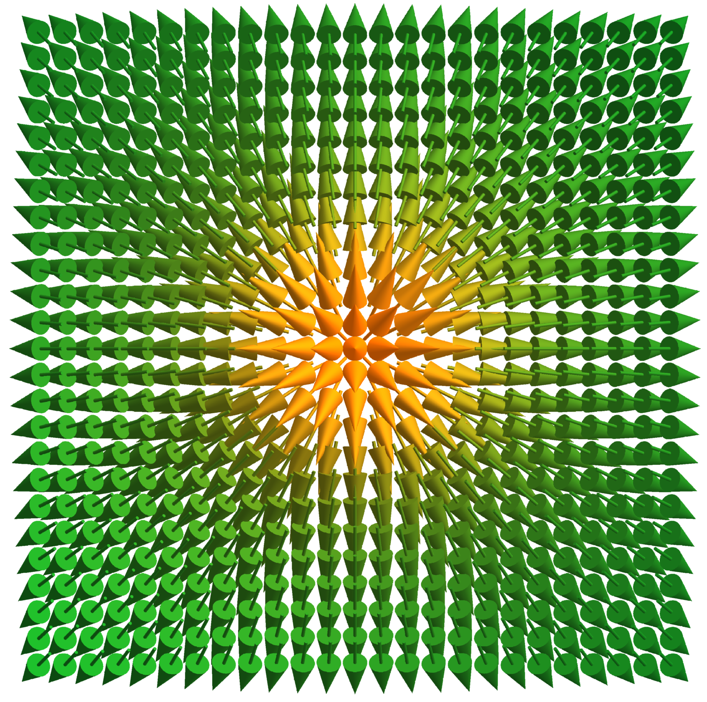
Figure 1: An outward Néel skyrmion, view from above (in the negative $z$-direction).

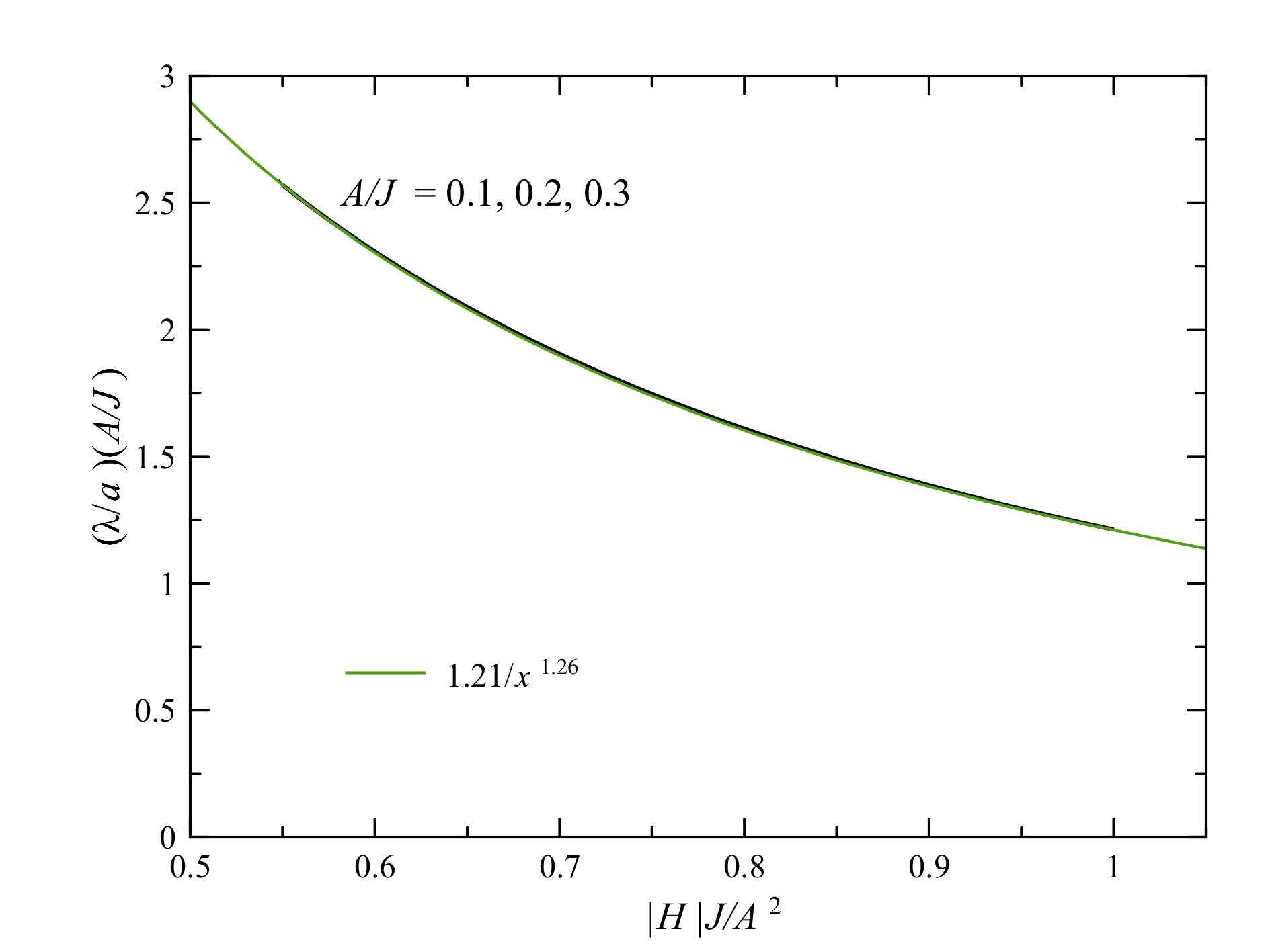
Figure 2: The scaled plot of the skyrmion size $\lambda$ vs. $H$ for different values of $A$.

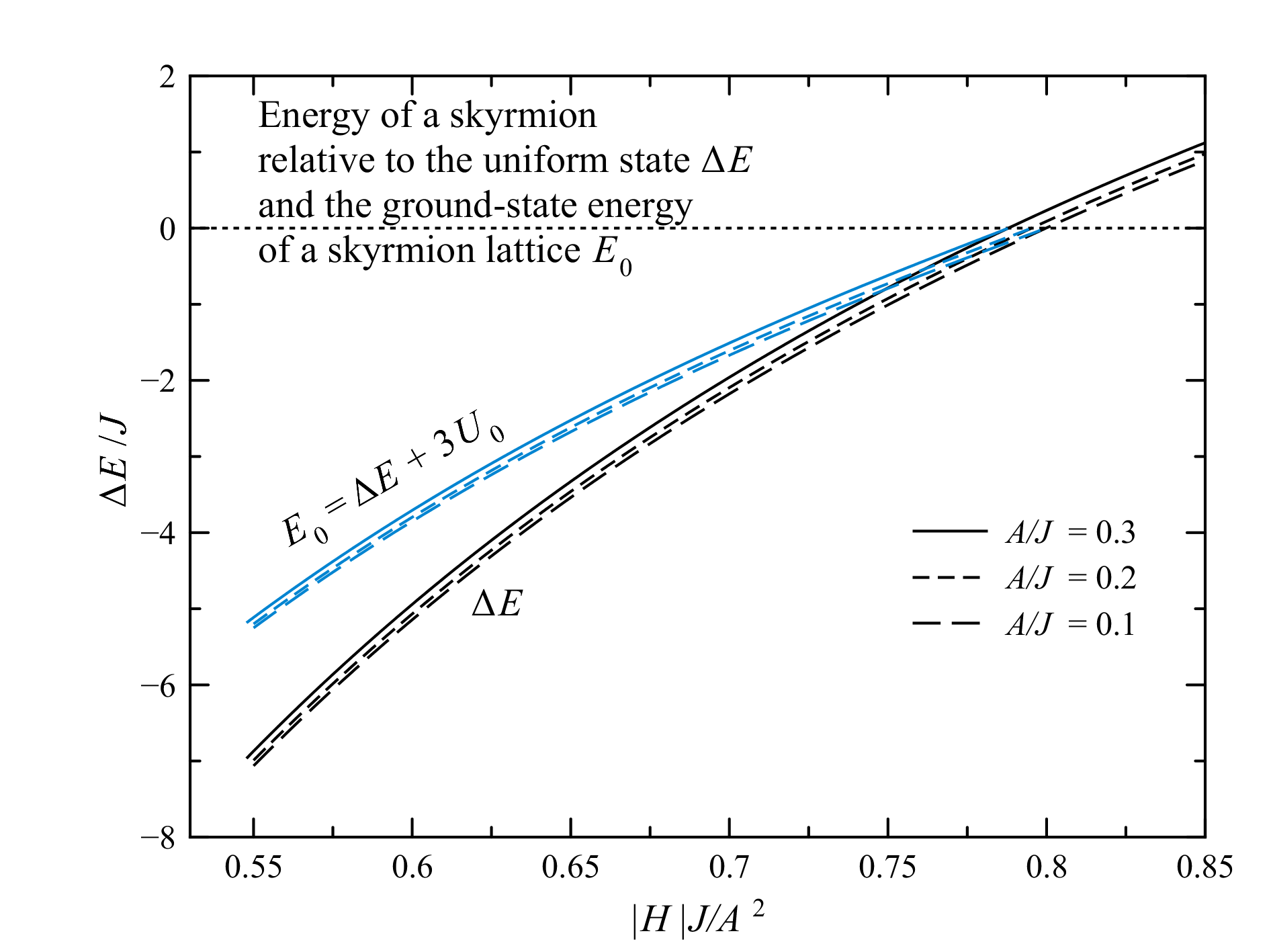
Figure 3: The energy of a single skyrmion $\Delta E$ with respect to the uniform state and the ground-state energy of an equilibrium skyrmion lattice per skyrmion $E_{0}$ vs $H$.

In the presence of the DMI, only skyrmions can exist as nontrivial topological states. The Néel-type DMI above favors outward skyrmions for $A>0$ (see Fig. 1), and inward skyrmions for $A<0$. There is another type of DMI that favors Bloch skyrmions. Most of the results are the same for both types of DMI. There is no analytical solution for the skyrmion’s profile $s_{z}(r)$ for the model with the DMI. In the numerical energy minimization on a lattice, the skyrmion size $\lambda$ can be defined using the formula [15]:

$$\lambda_{n}^{2}=\frac{n-1}{2^{n}\pi}a^{2}\sum_{i}(s_{i,z}+1)^{n},$$ (5)

that yields $\lambda_{n}=\lambda$ for the BP skyrmions for any $n$. For the computations, we took $n=4$ to give more weight to the skyrmion’s core.

To find the single-skyrmion spin configuration at $T=0$ numerically, one can start with a BP skyrmion or any topologically similar structure and perform energy minimization. Our numerical method combines sequential rotations of spins ${\bf s}_{i}$ towards the direction of the local effective field, ${\bf H}_{{\rm eff},i}=-\partial{\cal H}/\partial{\bf s}_{i}$, with the probability $\alpha$, and the energy-conserving spin flips (so-called overrelaxation), ${\bf s}_{i}\to 2({\bf s}_{i}\cdot{\bf H}_{{\rm eff},i}){\bf H}_{{\rm eff},i}/H_{{\rm eff},i}^{2}-{\bf s}_{i}$, with the probability $1-\alpha$. The parameter $\alpha$ plays the role of the effective relaxation constant. We mainly use the value $\alpha=0.03$ that provides the overall fastest convergence. We used the system dimensions $100\times 100$ for $A/J=0.3,$0.2 and $200\times 200$ for $A/J=0.1$. The scaled plot of the skyrmion size $\lambda$ vs $H$ for different values of $A$ is shown in Fig. 2. The skyrmion solution exists in the field interval $H_{s}\leq|H|\leq H_{c}$, where $H_{s}\simeq 0.55A^{2}/J$ is the “strip-out” field below which the skyrmion becomes unstable and converts into a laminar domain structure and $H_{c}\simeq 0.97A^{3/2}/J^{1/2}$ [64] is the skyrmion-collapse field. The ratio of the field boundary values is $H_{c}/H_{s}\simeq 1.76\left(J/A\right)^{1/2}$ that is greater than one for realistic parameters’ values.

The energy of a single skyrmion with respect to the uniform state becomes negative for $A$ large enough and $|H|$ small enough that makes the skyrmion thermodynamically stable, see black lines in Fig. 3.

II.2 Skyrmion-skyrmion repulsion and the equilibrium skyrmion lattice

Figure 4: Two repelling outward Néel skyrmions.

Skyrmions repel each other via two mechanisms. One is intrinsic repulsion via the conflicting in-plane spin fields created by the two skyrmions. This repulsion energy decreases exponentially on the distance $d$ between the skyrmions and has the form [63]

$$U(d)\simeq F\exp\left(-\frac{d}{\delta_{H}}\right),\qquad F\equiv 60J\left(\frac{A^{2}}{JH}\right)^{2},$$ (6)

where $\delta_{H}=a\sqrt{J/|H|}$ is the magnetic length. The formula above was obtained by fitting the numerical data for the skyrmion-skyrmion repulsion energy and is valid in a wide range of $A$ and $H$.

At large distances, the dominant interaction becomes the dipole-dipole repulsion proportional to the number of magnetic layers in the film and decaying as $1/d^{3}$, see Fig. 7 and Eq. (21) of Ref. [63]. Here, we will take into account only the strong short-range interaction and ignore the DDI repulsion.

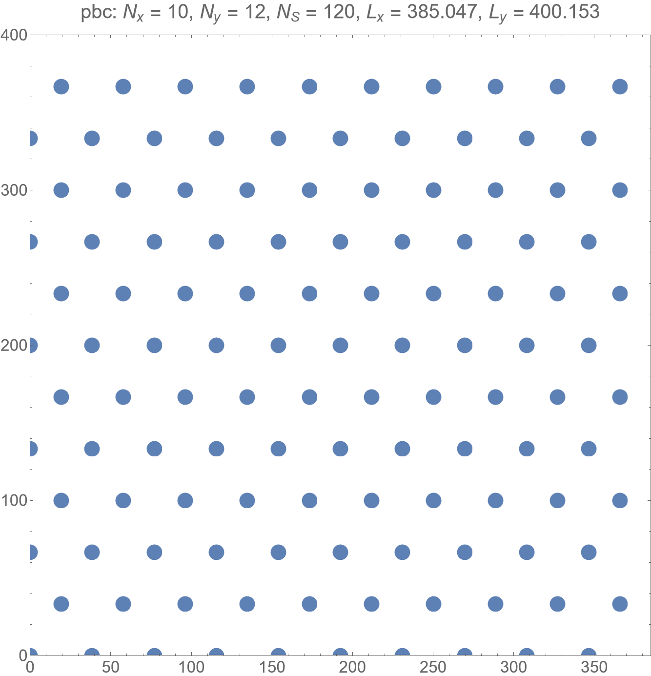
Figure 5: Triangular lattice of skyrmions in a nearly square system with periodic boundary conditions, $a_{S}=38.5a$.

The number if skyrmions in the system is not fixed and can be found, at least at low temperatures, from the minimization of the total system’s energy taking into account the skyrmion’s core energy $\Delta E$ and the skyrmion-skyrmion interaction energy. Consider a system of area $S$ containing a triangular skyrmion lattice of the period $a_{S}$, see Fig. 5. The unit cell is a rhombus of the area $a_{S}^{2}\cos 60\text{\textdegree}=a_{S}^{2}\sqrt{3}/2$, thus there are

$$N_{S}=\frac{2}{\sqrt{3}}\frac{S}{a_{S}^{2}}$$ (7)

skyrmions in the system. Each skyrmion in the lattice interacts with its six nearest neighbors, whereas, as we shall see, the interaction with further neighbors is negligibly small. Half of the interaction energy can be ascribed to each skyrmion in a pair. Thus, the energy per skyrmion is

$$E_{0}=\varDelta E+3F\exp\left(-\frac{a_{S}}{\delta_{H}}\right).$$ (8)

The equilibrium state is defined by the minimization of the total system’s energy $E_{\mathrm{tot}}=N_{S}E_{0}$ with respect to $a_{S}$ that leads to the transcendental equation

$$-\frac{\varDelta E}{3F}=\left(1+\frac{x}{2}\right)e^{-x},\qquad x\equiv\frac{a_{S}}{\delta_{H}}.$$ (9)

This transcendental equation has a solution for

$$0<-\varDelta E/(3F)<1$$ (10)

that is possible only for the negative skyrmion’s core energy $\varDelta E$. For $\varDelta E\rightarrow 0$, Eq. (9) yields $x\rightarrow\infty,$ then $E_{0}\rightarrow 0$.

Stability of the lattice requires $E_{0}<0$, that is, $-\varDelta E/(3F)e^{x}>1$. Using Eq. (9), one can eliminate the exponential and rewrite this condition as

$$-\frac{\varDelta E}{3F}e^{x}=1+\frac{x}{2}>1$$ (11)

that is trivially satisfied with $x>0$. That is, if Eq. (9) has a solution, then the energy of the skyrmion lattice is always negative, that is, it is below the energy of the uniform state.

As an illustration, for our main set of parameters $A/J=0.2$ and $H/J=-0.025$ one has $\varDelta E=-4.23J$, $\delta_{H}=6.32a$, and $F=154J$, thus $-\varDelta E/(3F)=0.009156$ and the solution of the transcendental equation yields $x=6.09$ and $a_{S}=38.5a$. In this case, the nearest-neighbor interaction energy

$$U_{0}=F\exp\left(-\frac{a_{S}}{\delta_{H}}\right)$$ (12)

becomes $U_{0}=Fe^{-x}=0.3486J$. The next-nearest-neighbor interaction energy is $U_{nnn}=Fe^{-\sqrt{3}x}=0.0040J$ and it is, indeed, negligible.

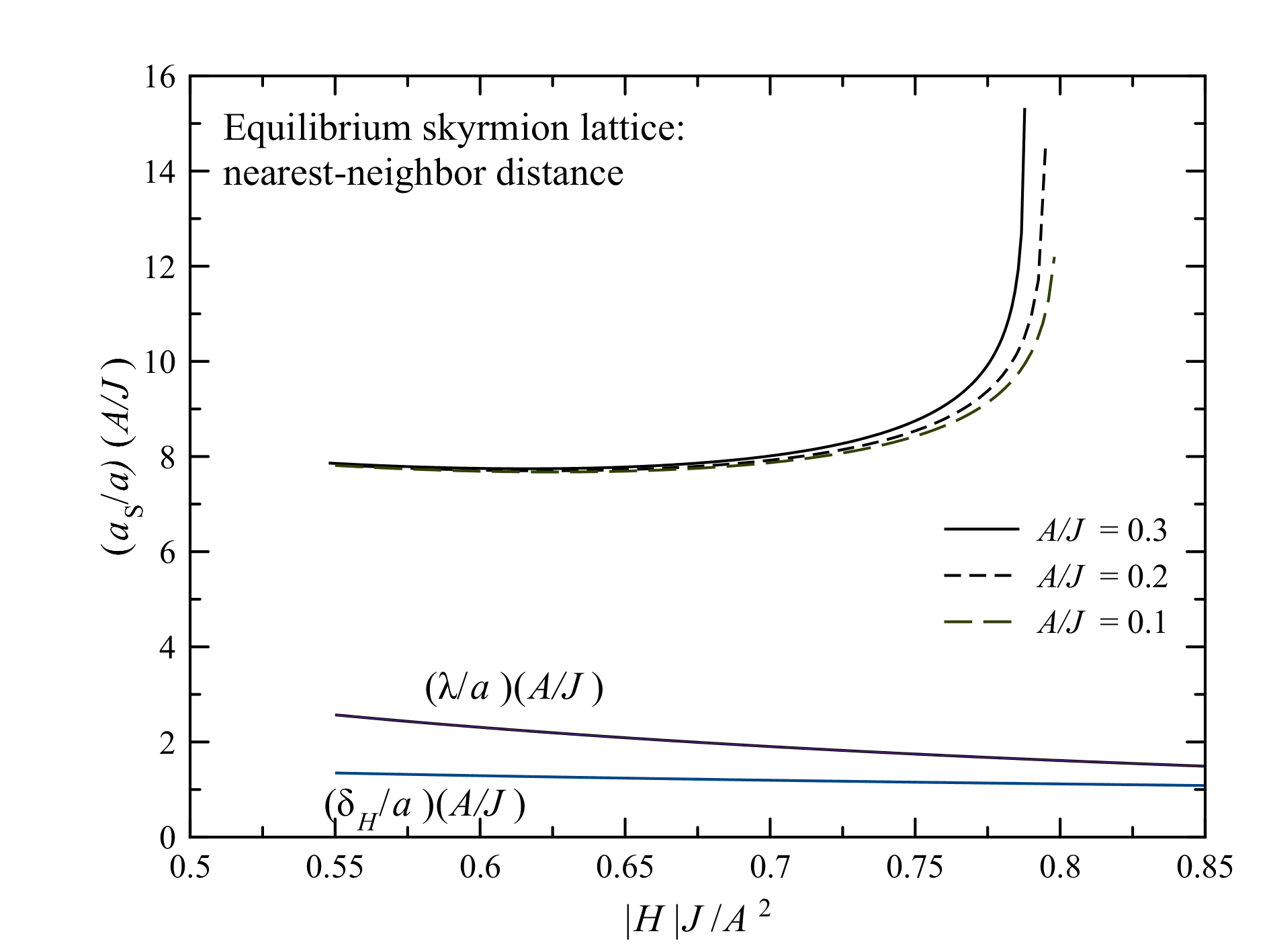
Figure 6: The equilibrium value of the skyrmion-lattice period $a_{S}$ vs $H$ for different values of $A$, compared with the skyrmion size $\lambda$ and the magnetic length $\delta_{H}$.

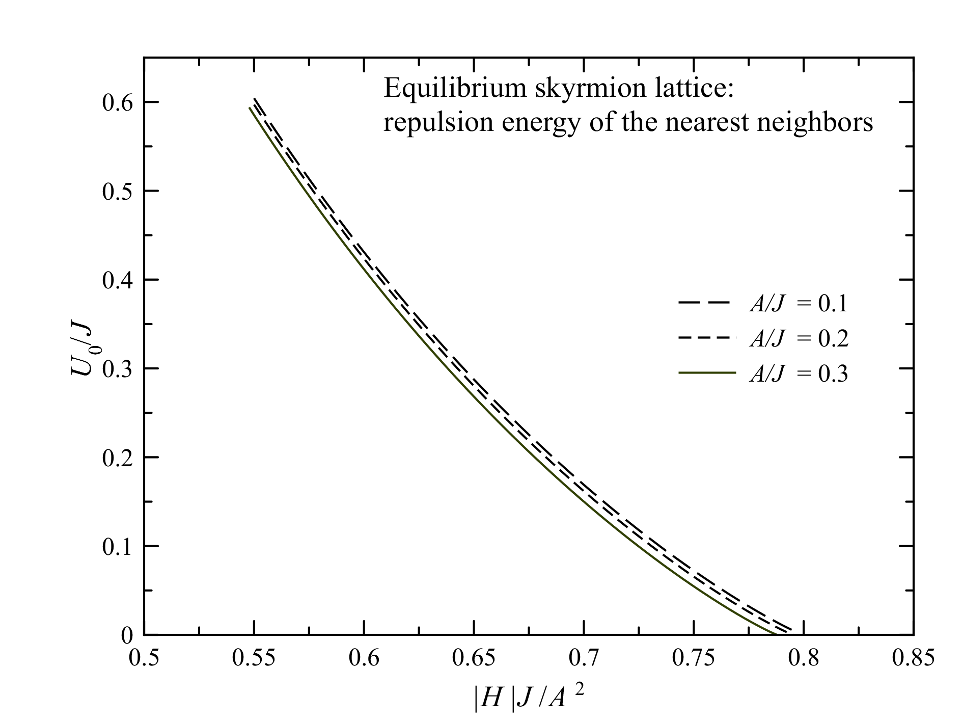
Figure 7: The nearest-neighbor repulsion energy $U_{0}$ in the equilibrium skyrmion lattice vs $H$ for different $A$.

The energy of the equilibrium skyrmion lattice per skyrmion $E_{0}$ is shown by the blue lines in Fig. 3 vs $H$ for different values of the DMI constant $A$. The values of $E_{0}$ are negative, as it should be. The calculated values of the skyrmion-lattice period $a_{S}$ are shown in Fig. 6. In the whole parameter range where skyrmions are stable, $a_{S}\apprge\lambda$ that allows to consider skyrmions as point objects. Near $|H|J/A^{2}\simeq 0.8$ where $\Delta E$ and $E_{0}$ vanish, $a_{S}$ is diverging. Finally, the skyrmion-skyrmion interaction energy $U_{0}$ in the skyrmion lattice is shown in Fig. 7. As near $|H|J/A^{2}\simeq 0.8$ the distance between skyrmions becomes large, the skyrmion interaction becomes small.

Although the number of skyrmions is not conserved and skyrmions can be created and annihilated, these processes are very unlikely at the temperatures near the melting point of the skyrmion lattice. For our main parameter set $A/J=0.2$ and $H/J=-0.025$, removing one skyrmion from the lattice increases the energy by $\Delta E_{-1}=-\Delta E-6U_{0}=2.14J$. Adding an additional skyrmion at the optimal position in the middle of any triangle increases the energy by $\Delta E_{1}=\Delta E+3F\exp(-r_{1}/\delta_{H})=9.48J$ if the interaction with the three nearest neighbors at the distance $r_{1}=a_{S}/\left[2\cos(30\text{\textdegree})\right]=22.2a$ at the corner of the triangle are taken into account. If the three next-nearest neighbors at the distance $44.5a$ are taken into account, one obtains $\Delta E_{1}=9.89J$. On the other hand, the melting temperature is $T_{m}\simeq 0.12J$, so that in the problem of melting a skyrmion lattice the high-energy processes changing the number of skyrmions can be neglected and the number of skyrmions can be kept constant. The equilibrium number of skyrmions found in this section establishes at higher temperatures when the temperature is lowered.

II.3 Constructing skyrmion lattices

We study skyrmion lattices in several typical geometries such as nearly square system with periodic boundary conditions (pbc), nearly square system with rigid walls, rhomboid system with rigid walls, and circular system with rigid walls. Positions of skyrmions in the basic triangular lattice are given by

$$\frac{{\bf R}}{a_{S}}={\bf e}_{x}n_{x}+\mathbf{e}_{60}n_{60}={\bf e}_{x}\left(n_{x}+\frac{1}{2}n_{60}\right)+{\bf e}_{y}\frac{\sqrt{3}}{2}n_{60},$$ (13)

where ${\bf e}_{x}$ and ${\bf e}_{y}$ are unit vectors along $x,y$ coordinate axes, $\mathbf{e}_{60}=(1/2){\bf e}_{x}+(\sqrt{3}/2){\bf e}_{y}$ is the lattice vector directed at $60\text{\textdegree}$ to $x$-axis and $n_{x}$, $n_{60}$, are integers. The regions of $n_{x},n_{60}$ and the dimensions of the system are chosen to avoid distortions of the lattice near the boundaries that is possible only for the pbc and rhombic system.

An example of the near-square pbc system is shown in Fig. 5. In this case, it is convenient to use $n_{x},n_{y}$ values in the intervals $1\leq n_{x}\leq N_{x}$ and $1\leq n_{60}\leq N_{y}$ with $N_{y}=2\mathrm{Int}(N_{x}/\sqrt{3})+2$, where $N_{y}$ is the number of rows in the lattice, and define the lattice points as

$$\frac{{\bf R}}{a_{S}}={\bf e}_{x}\left[n_{x}-1+\mathrm{Fr}\left(\frac{n_{y}-1}{2}\right)\right]+{\bf e}_{y}\frac{\sqrt{3}}{2}\left(n_{y}-1\right),$$ (14)

where $\mathrm{Int}(x)$ and $\mathrm{Fr}(x)$ are integer and fractional parts of $x$. The number of skyrmions in this lattice is $N_{S}=N_{x}N_{y}$. The system dimensions are chosen as

$$L_{x}=a_{S}N_{x},\qquad L_{y}=a_{S}\frac{\sqrt{3}}{2}N_{y}.$$ (15)

For large systems one has $L_{x}\cong L_{y}$ and the shape is close to a square. One can see in Fig. 5 that the system has a smooth periodicity in $x$- and $y$-directions.

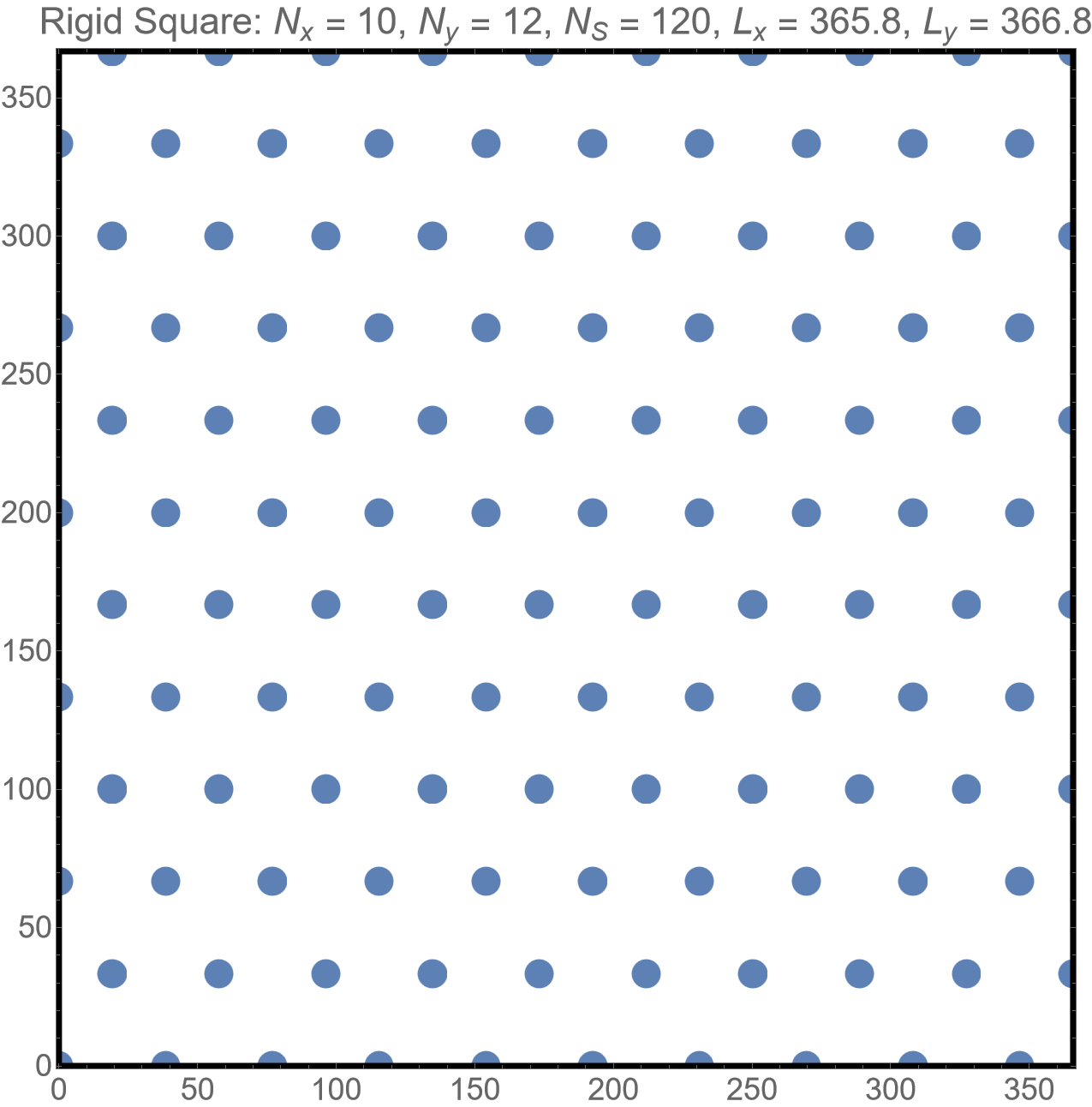
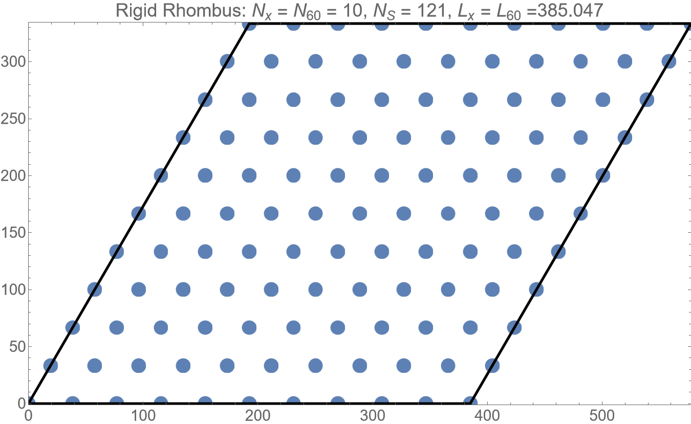
Figure 8: Triangular lattice of skyrmions in a nearly square and rhomboid systems with rigid boundaries.

A near-square triangular lattice with rigid boundaries is constructed in a similar way with minor modifications, see Fig. 8 (upper). Equation (14) and the definitions of $N_{x}$ and $N_{y}$ remain the same, while the system dimensions are given by

$$L_{x}=a_{S}\left(N_{x}-\frac{1}{2}\right),\qquad L_{y}=a_{S}\frac{\sqrt{3}}{2}\left(N_{y}-1\right).$$ (16)

In this system, the lattice becomes distorted near the vertical walls as the skyrmion in all rows will be pressed to the walls by the internal pressure resulting from the skyrmion repulsion.

For the system of a rhomboid shape with rigid boundaries, see Fig. 8 (lower), we use Eq. (13) with $0\leq n_{x},n_{60}\leq N_{x}$, so that there are $N_{S}=\left(N_{x}+1\right)^{2}$ skyrmions. The system dimensions are $L_{x}=L_{60}=a_{S}N_{x}$. In this case, the internal pressure is not distorting the lattice.

For the system of a circular shape, the boundaries favor different orientations of the lattice cells at different positions near the boundary that introduces frustration and makes a perfect triangular lattice impossible. In this case the system crystallizes into a polycrystalline state as the only possible scenario, see Fig. 9. However, for other system shapes a polycrystalline state also emerges on cooling, if the systems size is not too small.

III Physical quantities of triangular lattices

In this section, we define physical quantities that characterize the triangular lattice at zero and non-zero temperatures. Apart of the energy, in the focus of interest are orientational and translational orders.

III.0.1 Orientational order parameter and correlation function

The orientation of the hexagon of nearest neighbors of any particle $i$ in the lattice is quantified by local hexagonality [44]

$$\Psi_{i}=\frac{1}{6}\sum_{j}\exp(6i\theta_{ij}),$$ (17)

where the summation is carried out over 6 nearest neighbors $j$, $\theta_{ij}$ is the angle between the $ij$ bond and any fixed direction in the 2D lattice. If $\theta$ is counted from the direction of the $x$-axis (which is our choice), and two of the sides of the perfect hexagon coincide with the $x$-axis (the horizontal hexagon orientation), then all terms in the sum are equal one and $\Psi_{i}=1$. For any other orientation of a perfect hexagon, $\Psi_{i}$ is a complex number of modulus 1. In particular, the vertical hexagon orientation obtained by rotation by $30\text{\textdegree}$ from the horizontal orientation has $\Psi_{i}=-1$. The angle $\phi_{i}$ by which the hexagon $i$ is rotated from its initial horizontal orientation is related to the phase angle $\Theta_{i}$ in $\Psi_{i}=\left|\Psi_{i}\right|e^{i\Theta_{i}}$ by $\phi_{i}=\Theta_{i}/6$. At finite temperatures, orientations of the bonds fluctuate and the condition $|\Psi_{i}|=1$ no longer holds. One can introduce the hex value averaged over the system,

$$V_{6}=\sqrt{\left\langle|\Psi_{i}|^{2}\right\rangle_{i}}$$ (18)

that describes the quality of hexagons. At high temperature, when the order is completely destroyed, the orientations of the bonds and the angles $\theta_{ij}$ together with them become random. In this limit $\left\langle|\Psi_{i}|^{2}\right\rangle_{i}=1/6$ as each particle has six nearest neighbors on average. To describe the common orientation of hexagons in the lattice, one can introduce the orientational order parameter.

$$O_{6}=\langle\Psi_{i}\rangle_{i}.$$ (19)

Harmonic theory of 2D lattices yields a linear temperature dependence of $O_{6}$ at low temperatures [48]. As we will see, this linear decrease is due to the local disordering of individual hexagons described by $V_{6}$. It is thus more convenient to plot $O_{6}/V_{6}$ that describes the pure orientational order and only weakly depends on temperature at low $T$.

In Eq. (17) one can define nearest neighbors as those within a circle of radius $R_{0}$. A natural choice is $R_{0}=a_{S}\left(1+\sqrt{3}\right)/2$ that is the average between the nearest-neighbor distance and next-nearest-neighbor distance.

The orientational correlations in the lattice are defined as

$$C_{6,ij}=\frac{\mathrm{Re}\left(\Psi_{i}\Psi_{j}^{*}\right)}{\left\langle|\Psi_{i}|^{2}\right\rangle_{i}}.$$ (20)

To obtain the orientational correlation function (CF) that depends on the distance $r_{ij}\equiv\left|\mathbf{r}_{i}-\mathbf{r}_{j}\right|$, one has to compute all $C_{6,ij}$ values and corresponding distances in the system. Then one can put the data on the plot. However, for a large system there are too many plotting points. A better solution is to make a histogram by binning the distances $r_{ij}$ into the intervals of order $a_{S}$ and averaging $C_{6,ij}$ within each bin. We use the bin size exactly equal to $a_{S}$, although other choices are possible, too. One can see that the correlation function defined above, $C_{6}(r)$, is equal to 1 at $r=0$ that corresponds to $i=j$.

In the liquid or a polycrystalline state, $C_{6}(r)\rightarrow 0$ at $r\rightarrow\infty$. In this case one can use the finite-size value $O_{6}\propto 1/\sqrt{N_{S}}$ to estimate the corresponding correlation radius $R_{6}$. One has

$$\left|O_{6}\right|^{2}=\frac{1}{N_{S}^{2}}\sum_{ij}\Psi_{i}\Psi_{j}^{*}\Rightarrow\frac{1}{N_{S}}\int_{0}^{\infty}\frac{2\pi rdr}{a_{S}^{2}}C_{6}(r).$$ (21)

For the exponential CF, $C_{6}(r)=\exp\left(-r/R_{6}\right)$, one obtains

$$\frac{R_{6}}{a_{S}}=\left|O_{6}\right|\sqrt{\frac{N_{S}}{2\pi}}.$$ (22)

III.0.2 Cristallinity

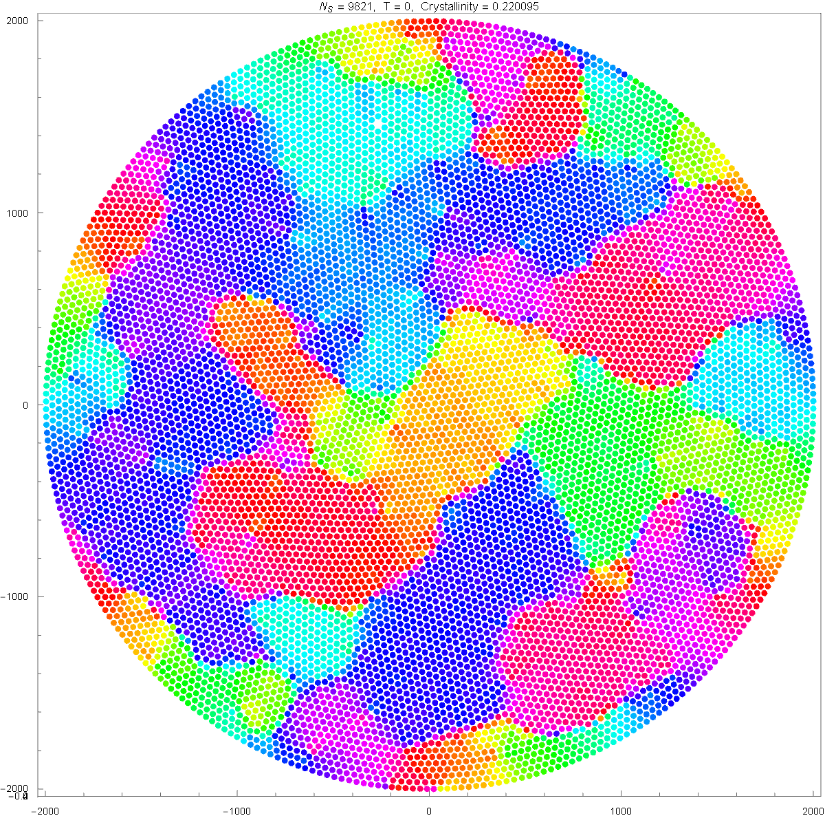
Figure 9: Polycrystalline structure of the skyrmion lattice in the magnetic film of circular shape with $N_{S}=9821$ skyrmions at $T=0$, obtained by cooling from high temperature.

Another measure of orientational order that we introduce here is cristallinity. Definition of crystallinity suggested below is based upon observation that in the case of a total disorder the phase $\Theta_{i}$ angle of $\Psi_{i}$ would be uniformly distributed in the interval $(-\pi,\pi)$. Consequently, a sorted list of the values of $\Theta_{i}$ plotted vs its index $i=1,2,...,N$ would be a straight line. Normalizing $\Theta_{i}$ by $2\pi$ and $i$ by the number of particles $N$ produces a straight line going from $(0,-0.5)$ to $(1,0.5)$. When differently oriented crystallites are present, the dependence of $\Theta_{i}$ on $i$ has plateaus in the ranges of $i$ that belong to the same crystallite or similarly oriented crystallites, while the plateaus are separated by narrow boundaries. This suggests definition of crystallinity as the deviation from the straight line mentioned above:

$$Crystallinity=\frac{4}{N}\sum_{i=1}^{N}\left|\Theta_{i}-\langle\Theta_{i}\rangle+\frac{i}{N}-0.5\right|,$$ (23)

where $\langle\Theta_{i}\rangle$ is the average phase angle in the system. This quantity can be easily computed after all $\Psi_{i}$ are found.

For a single crystal, $\Theta_{i}=\langle\Theta_{i}\rangle$, and the sum in Eq. (23) reduces to summation of the areas of two right-angle triangles, giving crystallinity of one. If the system splits into $k$ crystallites of equal size, with equidistant values of $\Theta$, crystallinity computed in a similar manner equals $1/k$. This provides an estimate for the average number of particles in a crystallite $N_{C}$ using $N_{C}/N=1/k$. In fact, one can define $N_{C}=Crystallinity\times N$.

It is convenient to show the polycrystalline state of a triangular lattice with color coding using the function $\mathrm{Hue}\left(\Theta_{i}/(2\pi)\right)$. As the argument of this function changes from 0 to 1, the color changes as red, yellow, green, cyan, blue, magenta, and red again. An example of a polycrystalline state in such a representation for a system of circular shape obtained by cooling to $T=0$ from a completely disordered state at $T=\infty$ is shown in Fig. 9. Figs. 5 and 8 could be color coded as red.

III.0.3 Translational order

The structure of the lattice is commonly described by the structure factor

$$S({\bf q})=\sum_{i}\exp(i{\bf q}\cdot{\bf r}_{i}).$$ (24)

For a perfect lattice, $\left|S({\bf q})\right|$ has sharp maxima at ${\bf q}$ equal to one of the reciprocal lattice vectors or their linear combinations. For the triangular lattice with horizontal hexagons ($\Theta_{i}=0$) there are three reciprocal-lattice vectors

$$\mathbf{q}_{1}=(0,1)q,\quad\mathbf{q}_{2}=\frac{(\sqrt{3},-1)}{2}q,\quad\mathbf{q}_{3}=\frac{(-\sqrt{3},-1)}{2}q,$$ (25)

where $q\equiv 4\pi/\left(\sqrt{3}a_{S}\right)$. One can check ${\bf q}_{\nu}\cdot{\bf R}_{i}=2\pi$ for $\nu=1,2,3$ and ${\bf R}_{i}$ being any particle position in a perfect lattice. This gives an idea to define the translational order parameter for a given configuration as

$$O_{\mathrm{tr}}\equiv\frac{1}{3N_{S}}\sum_{\nu=1}^{3}\left|\sum_{i}\exp(i{\bf q}_{\nu}\cdot{\bf r}_{i})\right|$$ (26)

that takes the value 1 for a perfect lattice and smaller values in the presence of defects or thermal excitations. To improve the statistic, we sum over all three reciprocal-lattice vectors.

In the same vein, translational correlations can be described by

$$C_{\mathrm{tr},ij}=\frac{1}{3}\sum_{\nu=1}^{3}\cos\left[{\bf q}_{\nu}\cdot\left({\bf r}_{i}-{\bf r}_{j}\right)\right].$$ (27)

Then, one can define the translational correlation function $C_{\mathrm{tr}}(r)$ in the same way as the orientational CF: computing the above expression for every $i$ and $j$ and binning the results.

From harmonic theory of 2D lattices follows that at any nonzero temperature there is no true long-range translational order as long-wavelength fluctuations make the correlation function a power law:

$$C_{\mathrm{tr}}(r)\propto\left(\frac{a_{S}}{r}\right)^{\eta},\qquad\eta\propto T$$ (28)

(see, e.g., Ref. [48]). Correspondingly, the translational order parameter is not a true order parameter as it decreases to zero in the thermodynamic limit. Expressing $O_{\mathrm{tr}}$via the CF above, one obtains

$$O_{\mathrm{tr}}^{2}=\frac{1}{N_{S}}\sum_{i}C_{\mathrm{tr}}({\bf r}_{i})\sim\left(\frac{a}{L}\right)^{\eta},$$ (29)

where $L$ is the linear system size.

The definition of the translational order above relies on the single-crystal structure of the lattice. Before computing in Eqs. (26) and (27), one has to find the reciprocal-lattice vectors. In the polycrystalline state, each crystallite has its own set of ${\bf q}_{\nu}$, so that translational order in the whole system cannot be defined.

Even in a single-crystal state at small but nonzero temperatures, translational order in 2D is washed out by long-wavelength fluctuations, so that $C_{\mathrm{tr}}(r)$ decreases as a power of $r$ and $O_{\mathrm{tr}}$ slowly decreases with the system size (see below). Still, one can treat $O_{\mathrm{tr}}$ as a quasi-order parameter.

III.0.4 Lattice defects

Lattice imperfections can be generated by frustrating boundaries, see Fig. 9, thermal excitations, etc. The most common ones are boundaries between crystallites (grain boundaries), vacancies, dislocations and disclinations.

Disclinations are centered at the lattice sites having five or seven nearest neighbors and they result in the hexagon orientations being different at any different point away from the disclination center. Disclination with $z=5$ can be seen as the result of cutting a wedge from a crystal with subsequent deforming the crystal to close the gap. Disclination with $z=7$ can be seen as the result of inserting a wedge of additional particles into the system. Thus, a single disclination is a topological object and it should severely reduce both orientational and translational order in the system.

Dislocations are incomplete rows of particles that end at the dislocation center. A single dislocation can severely reduce the translational order but only slightly disturbs the orientational order. According to the common view, dislocations can be born in tightly-bound pairs by thermal agitation and then the pairs unbind at some temperature. Further, according to the KTHNY scenario, an isolated dislocation consists of a pair of disclinations that unbind at another still higher temperature.

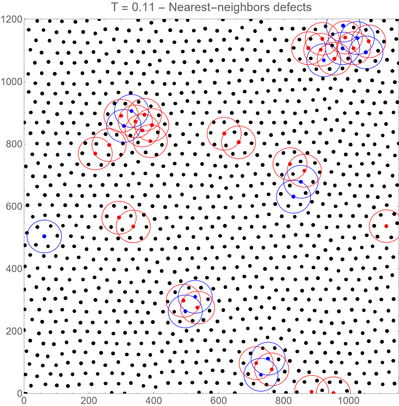
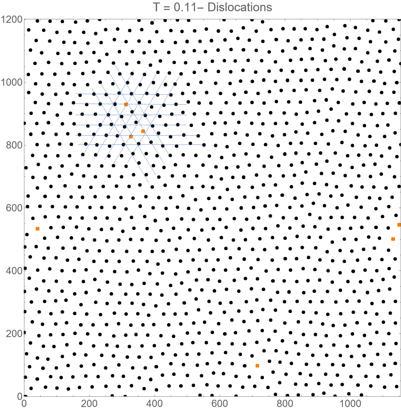
Figure 10: Skyrmion lattice at $T/J=0.11$. Upper panel: “disclinations” found by computing the number of nearest neighbors. Skyrmions with 5 and 7 nearest neighbors are marked by blue and red points and encircled by blue and red circles of radius $R_{0}=a_{S}\left(\sqrt{3}+1\right)/2$. Lower panel: “dislocations” found by computing the Burgers vector shown by orange squares.

At $T=0,$ finding dislocations and disclinations is relatively straightforward. Disclinations are found by counting the number of nearest neighbors for each lattice site. Dislocations can be found by computing the Burgers vector for each site. The numerical method is the following. As a preliminary, for each lattice site $i$ the local orientation of the lattice in its vicinity is found. For this,$\Psi_{j}$ is computed for the site $i$ and all its neighbors within the cutoff radius. For each of these sites, the phase angles $\Theta_{j}$ corresponding to $\Psi_{j}$ are found and averaged. Dividing the result by 6, as explained below Eq. (17), one obtains the average orientation of the lattice in the vicinity of $i$. After that, a minimal rhomboid trajectory around the site is constructed as follows. First, the point expected as the bottom-left corner of the rhombus in a perfect lattice is set and the particle closest to this point is found by checking all candidates. Then the point shifted by one lattice spacing in the positive $x$-direction from the found particle’s position is set and the particle closest to it is found. This step is repeated to find the bottom-right corner of the rhomboid trajectory. After that two similar steps are performed in the positive $60\text{\textdegree}$ direction to find the upper-right corner of the rhombus. Then two steps are done in the negative $x$-direction to find the upper-left corner of the rhombus. Finally, two steps are done in the negative $60\text{\textdegree}$ direction to return to the bottom-left corner of the rhombus. If the location of the latter coincides with that found at the beginning, there is no dislocation. If one comes to another site in the lattice, the Burgers vector is nonzero and there is a dislocation.

Whereas the procedure of finding dislocations and disclinations at $T=0$ is straightforward, it become ambiguous at elevated temperatures because of thermal shifting of particles from their equilibrium positions, see Fig. 10 (upper). Local displacements of neighbors of a site $i$ can result in the neighbor count different from six without any change in the system’s topology as a real disclination does. Furthermore, the neighbor count at elevated temperatures substantially depends on the choice of the range $R_{0}$ used for counting nearest neighbors. A small increase of $R_{0}$ above the typical value $R_{0}=a_{S}\left(1+\sqrt{3}\right)/2$ substantially increases the number of sites with seven neighbors and decreases the number of sites with five neighbors. This means that the number of nearest neighbors is not well defined at elevated temperatures. As the disclination is not a local but a global object, the method of their identification has to be global, too. However, non of such methods is currently known.

Similarly, numerical identification of tightly bound dislocation pairs at $T>0$ is unclear. Concerning isolated dislocations, one can compute Burgers vectors as explained above but one can get false positives because of too strong local thermal shifting of lattice sites from their expected positions without any actual dislocation, see Fig. 10 (lower). Ambiguities in identification of lattice defects at elevated temperatures are also mentioned on page 4 of Ref. [55]. It seems that direct checking of the KTHNY scenario of 2D melting by observing processes with dislocations and disclinations is problematic.

IV Numerical method

We compute the properties of the skyrmion lattice at nonzero temperatures $T$, including melting, using the Metropolis Monte Carlo (MC) method. All computations are performed for the set of parameters listed in Sec. II.2 [see above Eq. (12)].

The first thing to say is that the phase space of the system is very complicated and there are valleys separated by high barriers, so that thermally activated transitions between the valleys take a prohibitively long time at low $T$, practically below the melting point. As an example one can name the single-crystal state and polycrystalline states, see Fig. 9. The Monte Carlo routine reflects this property, that is, in general, it does not lead to averaging over different valleys and the numerical results belong to a particular valley.

In the Metropolis Monte Carlo, particles $i$ are successively displaced by a random vector $\Delta\mathbf{r}_{i}$ within the plane and the change of the energy $\Delta E_{i}$ is computed. The move is accepted if $\exp\left(-\Delta E_{i}/T\right)>\mathrm{rand}$, where rand is a random real number in the range (0,1), otherwise it is rejected. The trial displacement $\Delta\mathbf{r}_{i}$ should be essentially smaller than the lattice period $a_{S}$ to prevent a one-move destruction of the lattice. We used $\Delta\mathbf{r}_{i}$ in a random direction with the length $\left|\Delta\mathbf{r}_{i}\right|=\mathrm{MCD}\,a_{S}\left(T/U_{0}+0.1\right)\mathrm{rand}$, with the MC distance factor $\mathrm{MCD}=0.25$ and rand being a random real number in the range (0,1). With $U_{0}=0.3486J$ and the maximal temperature of the simulations $T_{\max}=0.2J$, the condition $\left|\Delta\mathbf{r}_{i}\right|\ll a_{S}$ is fulfilled everywhere. The average MC acceptance rate was about 0.65 at all temperatures except the lowest ones.

MC simulations were performed with Wolfram Mathematica with compilation in C on three different computers, the best of which, a Dell Precision workstation, has 16 cores available for Mathematica. Simulations at different $T$ were done in parallel cycles to maximize the usage of computing resources and gain more statistics. For each temperature in a cycle, we started with the same initial state using the perfect lattice initial condition (LIC) or random initial condition (RIC). The main body of computations was done for the system with pbc (see Fig. 5) with $N_{x}=300$ and thus the number of skyrmions $N_{S}=104400$. Another system size we used was $N_{x}=100$ with $N_{S}=11600$. Some simulations were performed for the nearly-square system with rigid walls [see Fig. 8 (upper)] and same sizes. Also, we have done simulations for the rhomboid system [see Fig. 8 (lower)] and for the circular system (see Fig. 9).

The relaxation (thermalization) time near the melting point turns out to be extremely long. For this reason, it is not feasible to perform Monte Carlo simulations with a fixed number of Monte-Carlo steps (MCS). Thus, one needs a MC routine with an automatic number of MCS defined with the help of some stopping criterion. We looked at the evolution of the system’s energy $E$ that was computed with the interval of $\mathrm{MCBlock}=10$ MCS. We define the running average of the energy $E_{\mathrm{mean}}$ being the mean of the last $\mathrm{Round}(\mathrm{MCMass\,}N_{E})$ output values of energy, where $N_{E}$ is the total number of the energy values and we used $\mathrm{MCMass}=0.3$ (that is, we averaged the last 30% of the obtained energy values). The value of $E_{\mathrm{mean}}$ that is much smoother than $E$ was used to formulate the stopping criterion as follows. We define the MC span, typically $\mathrm{MCSpan}=300$, and consider the last MCSpan values of the $E_{\mathrm{mean}}$ list. Then we define the slope of the energy $E_{\mathrm{slope}}$ per MCS using the averages of the first and second halves of the MCSpan list. The stopping criterion used reads $\left|E_{\mathrm{slope}}\right|<\mathrm{MCSens}\,U_{0}$, where MCSens is the MC sensitivity. The parameter $\mathrm{MCSens}$ takes very small values, from $10^{-7}$ down to $10^{-11}$. The minimal number of MCS is $\mathrm{MCBlock}\times\mathrm{MCSpan}$, typically 3000. The maximal number of MCS was set to $10^{6}$. To prevent stopping in the case when $E_{\mathrm{slope}}$ simply changes its sign, the stopping criterion was required to be fulfilled 10 times.

In many Monte Carlo simulations of the past, a large number of MCS was done to reach equilibrium and then another large number of MCS was used for the measurements of physical quantities in the equilibrium state. The second stage is needed for small systems to average out fluctuations. However, in large systems the measurement routine is unnecessary since for most quantities (except, for instance, susceptibility computed via the fluctuation formula) fluctuations within a particular valley are suppressed by self-averaging while averaging over different valley requires too much time and is not happening anyway. Thus for a large system, one can use just the final state after stopping the MC routine to compute physical quantities. Here, we used Monte Carlo with and without measuring stage and we have seen the effect of the measurement stage only for small systems above melting.

In the computation of the skyrmion-skyrmion interaction, we used the cutoff distance $r_{\mathrm{cutoff}}=0.95\sqrt{3}a_{S}$ that is just shy of the next-nearest distance $\sqrt{3}a_{S}$. For our set of parameters, nearest-neighbors interaction is $U_{0}=0.3486J$ while the interaction at the cutoff distance is $U_{\mathrm{cutoff}}=F\exp\left(-r_{\mathrm{cutoff}}/\delta{}_{H}\right)=0.00685J$ that is sufficiently small. Limiting the summation over interacting partners can be done by two methods.

First, for each particle, a list of particles within a range longer than $r_{\mathrm{cutoff}}$ is maintained. The interaction energy is computed by summation over these lists, whereas only the neighbors within the range $r_{\mathrm{cutoff}}$ are taken into account. The displacement of particles is monitored and the lists of prospective partners are updated from time to time. This method works well below melting as the particles remain near their initial places and the lists of partners do not need to be updated. However, in the liquid phase particles are traveling and the lists of partners have to be updated more and more frequently as the temperature increases. In fact, for large systems one needs to use several nested generations of partners’ lists as updating such list scanning the whole system take much time. So, it is better to choose partners from a larger partners’ list. Maintaining high-order lists of partners of each particle containing thousands of partners takes up a lot of memory. Thus, for large systems above melting this method becomes problematic. An example of a result obtained with the partner-lists method is Fig. 9.

Another method consists in splitting the system in regular bins, rectangular for the the systems of rectangular shape and rhomboid for the rhomboid system (see Fig. 8). Binning the system, that is, finding the number and positions of particles in each bin, is a fast procedure, and binning does not require too much memory. To compute the interaction energy for each particle, one needs to check for the prospective partners within the same bin and all neighboring bins, in total, in nine bins. The smaller the bins, the less partners are to check and the faster is the computation. However, the sizes of the bins have to exceed $r_{\mathrm{cutoff}}$. This method is slower below melting then the first one but it works better overall. The binning procedure is performed after each MCS. The most of the results are obtained by this second method.

Dislocations in the lattice are detected by computing the Burgers vector for each skyrmion, as explained in Sec. III.0.4.

V Numerical results

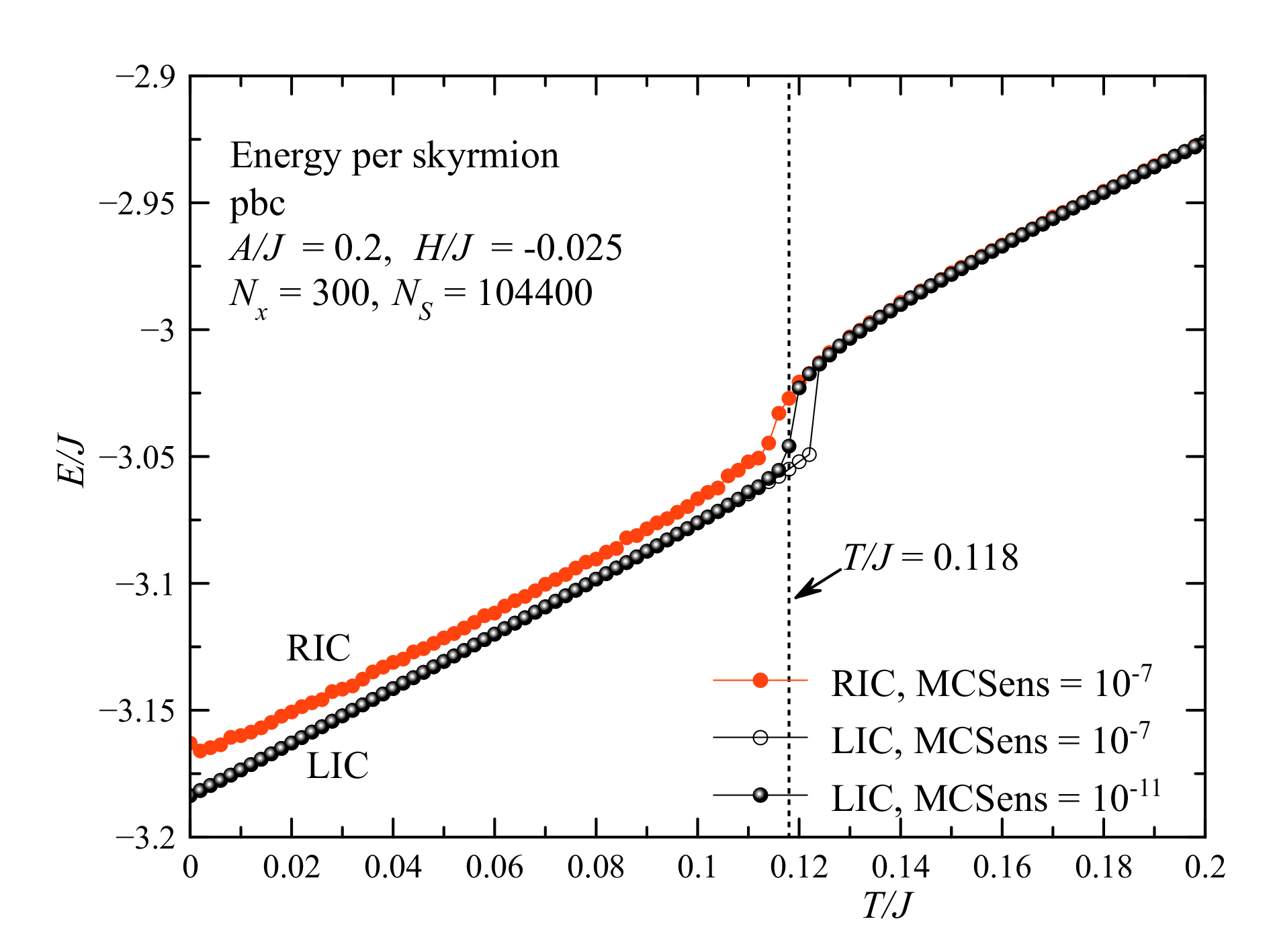
Figure 11: Temperature dependence of the energy per skyrmion $E$ for the lattice and random initial conditions with different Monte Carlo sensitivities.

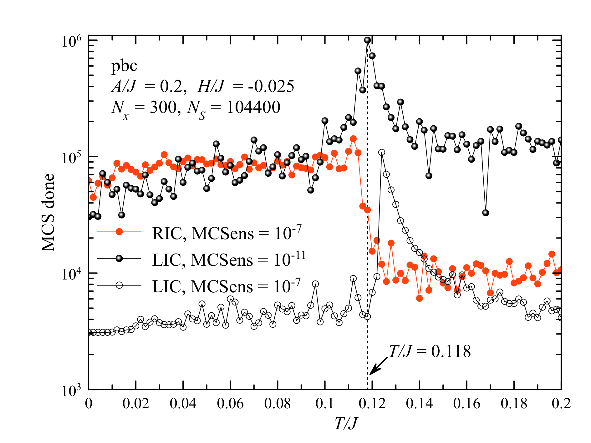
Figure 12: Temperature dependence of the number of Monte Carlo steps done.

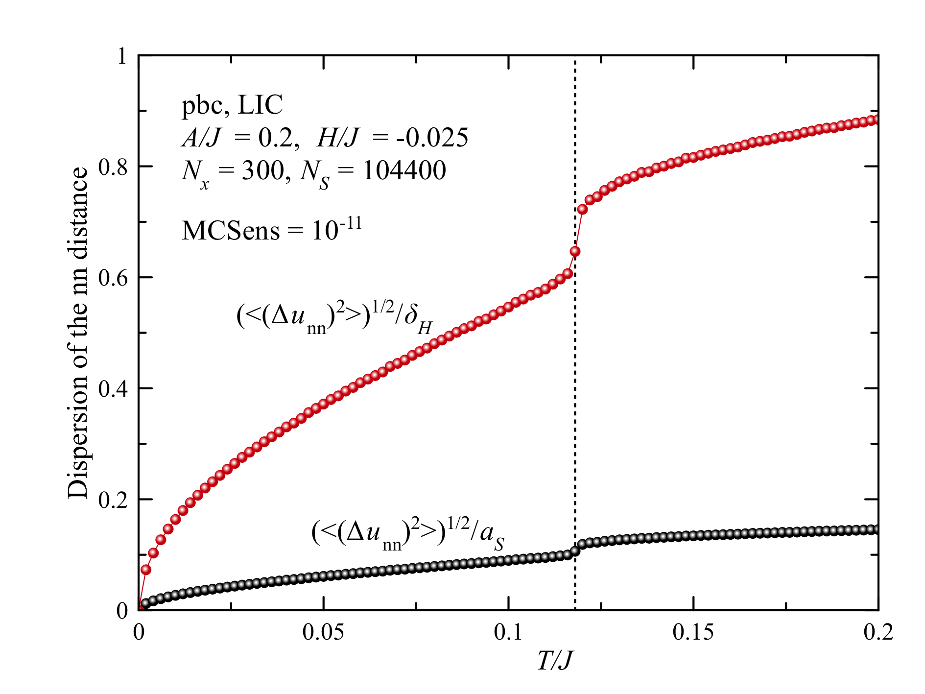
Figure 13: Temperature dependence of the dispersion of the nearest-neighbor distance in the skyrmion lattice.

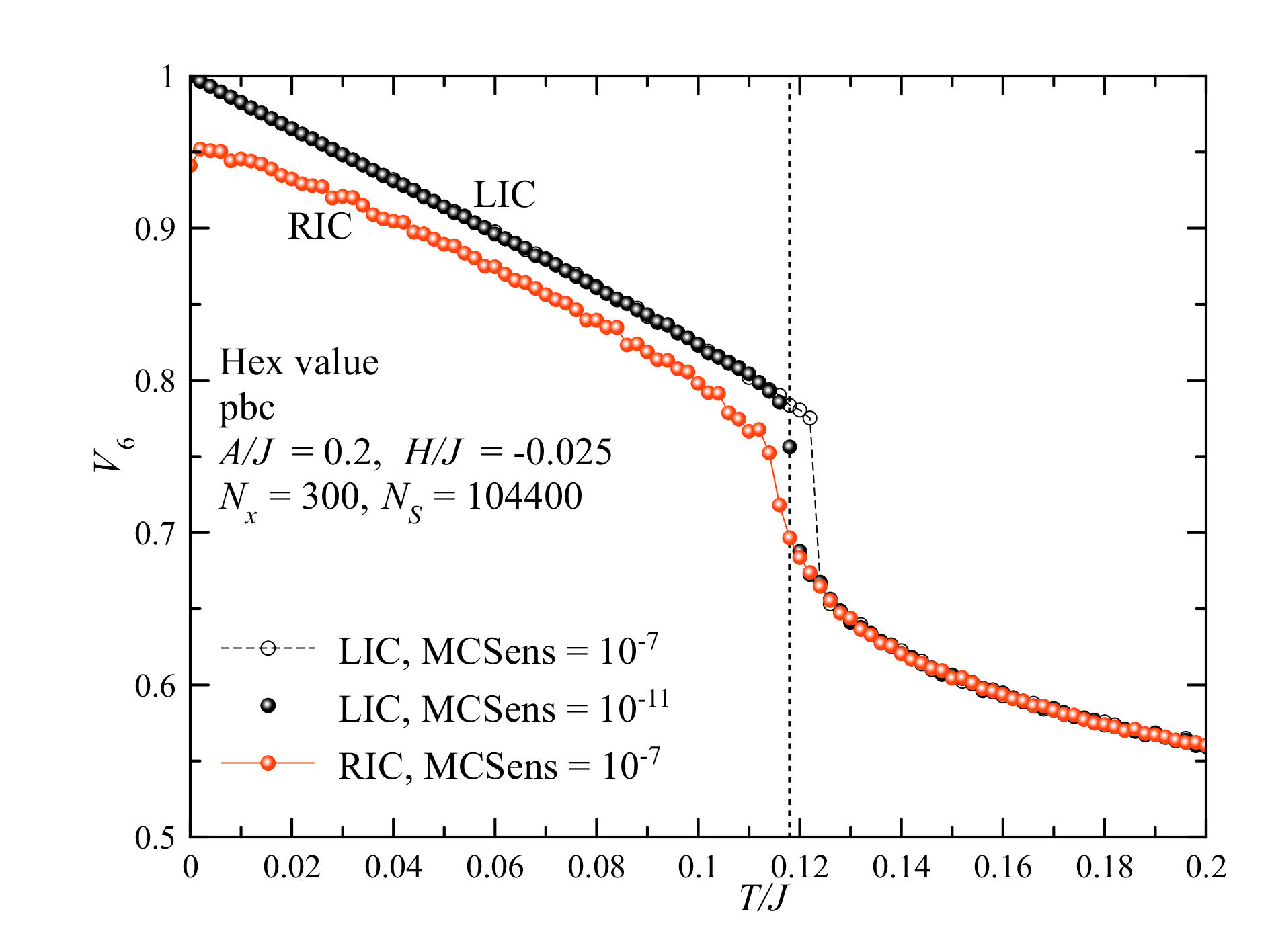
Figure 14: Temperature dependence of the average hexagonality value $V_{6}$, Eq. (18).

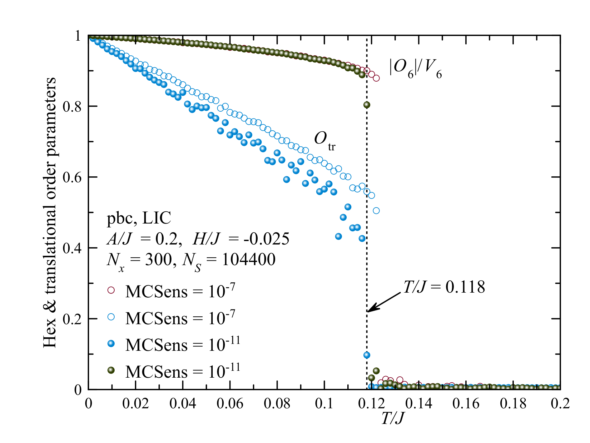
Figure 15: Temperature dependence of translational and orientational order parameters in a nearly-square skyrmion lattice with pbc.

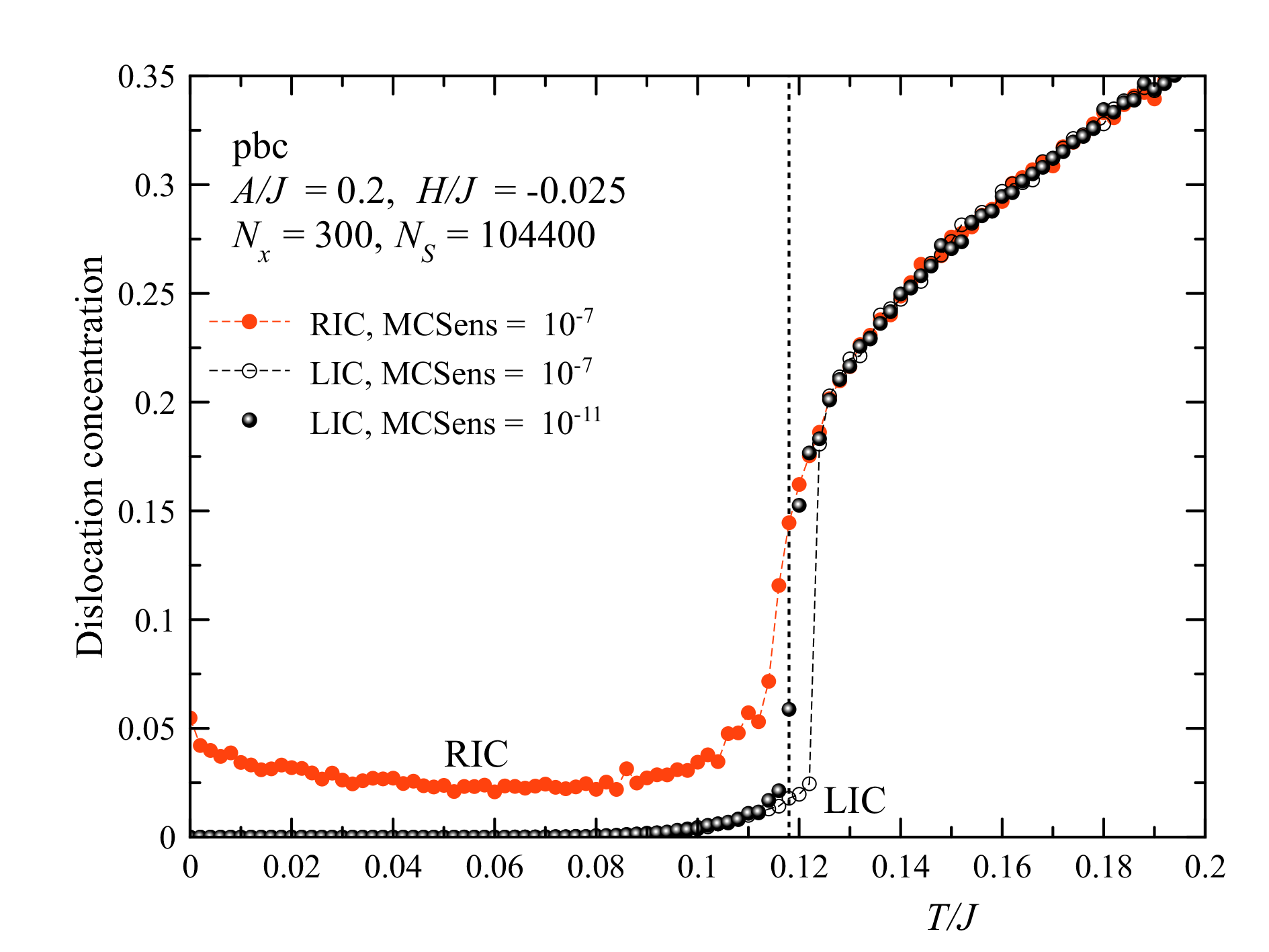
Figure 16: Temperature dependence of the concentration of dislocations, computed via the Burgers vector.

Figure 17: Temperature dependence of translational and orientational order parameters in a rhomboid skyrmion lattice with rigid boundaries, Fig. 8 (lower), with different system sizes. The dashed vertical line marks the approximate melting temperature for the pbc system, $T/J=0.118$.

The main question in the melting of the skyrmion lattice is the same as for all 2D systems: is the transition similar to that in 3D or there are two successive transitions mediated by dislocation and disclinations according to the KTHNY scenario? The results obtained show only one transition that seems to be a first-order transition and has a hysteresis with a big jump of physical quantities at the melting point. The position of the jump on $T$ slightly depends on the length of the Monte Carlo process, shifting to the left with the number of MCS done.

Temperature dependence of the order parameters for the system of rhomboid shape with rigid boundaries, Fig. 8 (lower), is shown in Fig, 17 for different system sizes. This system shape favors the horizontal hexagon orientation by the directions of its boundaries. The existence of this preferred hexagon orientation is seen in the tail of $O_{6}$ in the liquid phase. This tail does not exist in the model with pbc, Fig. 15, that does not set any preferred hexagon orientation. The tail is very pronounced for small system sizes and weakens for larger systems. This situation is resembling of a ferromagnetic system with a magnetic field applied at the boundary. As one can see in the picture, rigid boundaries also affect the translational order in finite-size systems, inducing a partial ordering above the melting point. The tail of $O_{\mathrm{tr}}$ also weakens with the system size, as expected. The melting temperature of the finite-size rhomboid system shifts to the right in comparison with the pbc system because of the stabilizing effect of the boundaries.

V.1 Temperature dependence of physical quantities in melting/freezing of the skyrmion lattice

The results for the three main systems studied here, near-square pbc system, near-square rigid-boundary system, and rhomboid rigid-boundary system are similar except for some subtleties that will be discussed later. So, we show mainly the results of the pbc system with $\sim 10^{5}$ skyrmions. The energy per skyrmion $E$ that contains the core energy $\Delta E<0$ and the positive repulsion energy is shown in Fig. 11. The energy values obtained starting from the perfect lattice (LIC) for both sets of the MC parameters, $\mathrm{MCSens}=10^{-7}$ with $\mathrm{MCSpan}=300$ and $\mathrm{MCSens}=10^{-11}$ with $\mathrm{MCSpan}=3000$ are the same everywhere except for the vicinity of the melting point. Data for $\mathrm{MCSens}=10^{-7}$ show a jump at $T/J=0.122$ while the data $\mathrm{MCSens}=10^{-11}$ show a jump at $T/J=0.118$. This implies that melting is driven by thermal activation over an energy barrier leading to nucleation of the liquid phase, as in 3D. The energy values obtained starting from random initial conditions (RIC) show a smaller jump at a lower temperature, and the energy values below melting are higher than in the case of LIC. The reason is that the system is freezing into a polycrystal state, so that grain boundaries and other defects increase the system’s energy. Longer simulation can slightly reduce the energy but formation of a single crystal in a large system required an exceedingly large time. For realistic systems, formation of a single crystal will be prevented by frustrating boundaries favoring different orientations of the hexagons (see, e.g., Fig. 9) and by pinning.

Fig. 12 shows the number of MCS done before the thermalization routine stopped. For the LIC data, thermalization at low temperatures is the shortest, with the numbers of MCS about their minima $\mathrm{MCSpan}\times\mathrm{MCBlock}$, that is, about $3000$ and 30000, respectively. Near the melting point, thermalization becomes very slow, especially above melting where the system’s state changes significantly. For the second simulation, the number of MCS reaches its cap of $10^{6}$ at $T/J=0.118$ without fulfilling the stopping criterion. In the case of RIC, the relaxation is very slow everywhere below freezing because of the slow motion of grain boundaries.

Temperature dependence of the dispersion of the nearest-neighbor distance in the skyrmion lattice $\sqrt{\left\langle\mathbf{u}_{nn}^{2}\right\rangle}$ is shown in Fig. 13. It increases as $\sqrt{T}$ at low temperatures, as expected from the theory of a harmonic lattice. There is a jump of the dispersion at the melting point. The two curves are normalized by $a_{S}$ and by the magnetic length $\delta_{H}$. The well-known empirical Lindemann criterion predicts melting when the dispersion of the distances becomes comparable with the lattice period. Practically, most of materials melt at a lower temperature when the dispersion is about 0.1 of the lattice period. Here, $\sqrt{\left\langle\mathbf{u}_{nn}^{2}\right\rangle}\simeq 0.1a_{S}$ at the melting point. The dispersion normalized by $\delta_{H}$ is of order one near melting. One can show this is the condition for anharmonic terms in the expansion of the skyrmion lattice energy to be comparable with the harmonic terms.

Fig. 14 shows the temperature dependence of the hex value $V_{6}$ defined by Eq. (18). In the LIC case, it linearly decreases with $T$ at low temperatures and jumps down at the melting point. Note that there is still a considerable hexagonality in the liquid phase above melting. In the RIC case, $V_{6}$ is below one at low $T$ because of lattice defects.

Probably, the most interesting are the results for the rotational and translational order parameters in the LIC case shown in Fig. 15. The main (linear) temperature dependence of $O_{6}$, Eq. (19), is due to the decrease of the hex value $V_{6}$, so we plot $\left|O_{6}/\right|V_{6}$ that describes the loss of hexagon’s orientations with temperature. This quantity goes quadratically at low $T$ and remains large until melting, where it jumps down to zero. The curves for $\mathrm{MCSens}=10^{-7}$ and $10^{-11}$ are in a good agreement everywhere except the vicinity of the melting point.

To the contrast, the corresponding results for the translational order parameter $O_{\mathrm{tr}}$, Eq. (26), differ significantly. While the $\left|O_{6}/\right|V_{6}$ are smooth below melting, those for $O_{\mathrm{tr}}$ show a large scatter. This confirms that $O_{\mathrm{tr}}$, unlike $O_{6}$, is not a good thermodynamic order parameter. There is only a translational quasi-order smeared by long-wavelength fluctuations and going to zero in the thermodynamic limit. Here we show that for a large but finite system $O_{\mathrm{tr}}$ exists but is difficult to compute as its convergence with the number of MCS is very slow. Also, $O_{\mathrm{tr}}$ is extremely sensitive to lattice defects, and a single dislocation or disclination in a large system can strongly reduce its value. Note that a longer thermalization creates more scatter in $O_{\mathrm{tr}}$, apparently due to thermal creation of lattice defects that is a slow process.

Finally, the temperature dependence of the concentration of dislocations $N_{\mathrm{disl}}/N_{S}$ computed in the same simulations via the Burgers vector as explained in Sec. III.0.4 is shown in Fig. 16. In the LIC case, the concentration of dislocations is very small at low temperatures, then increases and makes an upward jump at the melting point. Above melting it continues to increase and takes values of order one that should be characteristic of a liquid state. In the RIC case, the concentration of dislocations does not go to zero at $T\rightarrow 0$. These results should be taken with a grain of salt. As explained in Sec. III.0.4, there should be false positives because of local lattice distortions that are not real dislocations. Similarly, it is easy to compute the concentration of skyrmions having 5 or 7 neighbors but at elevated temperatures it does not prove the existence of disclinations.

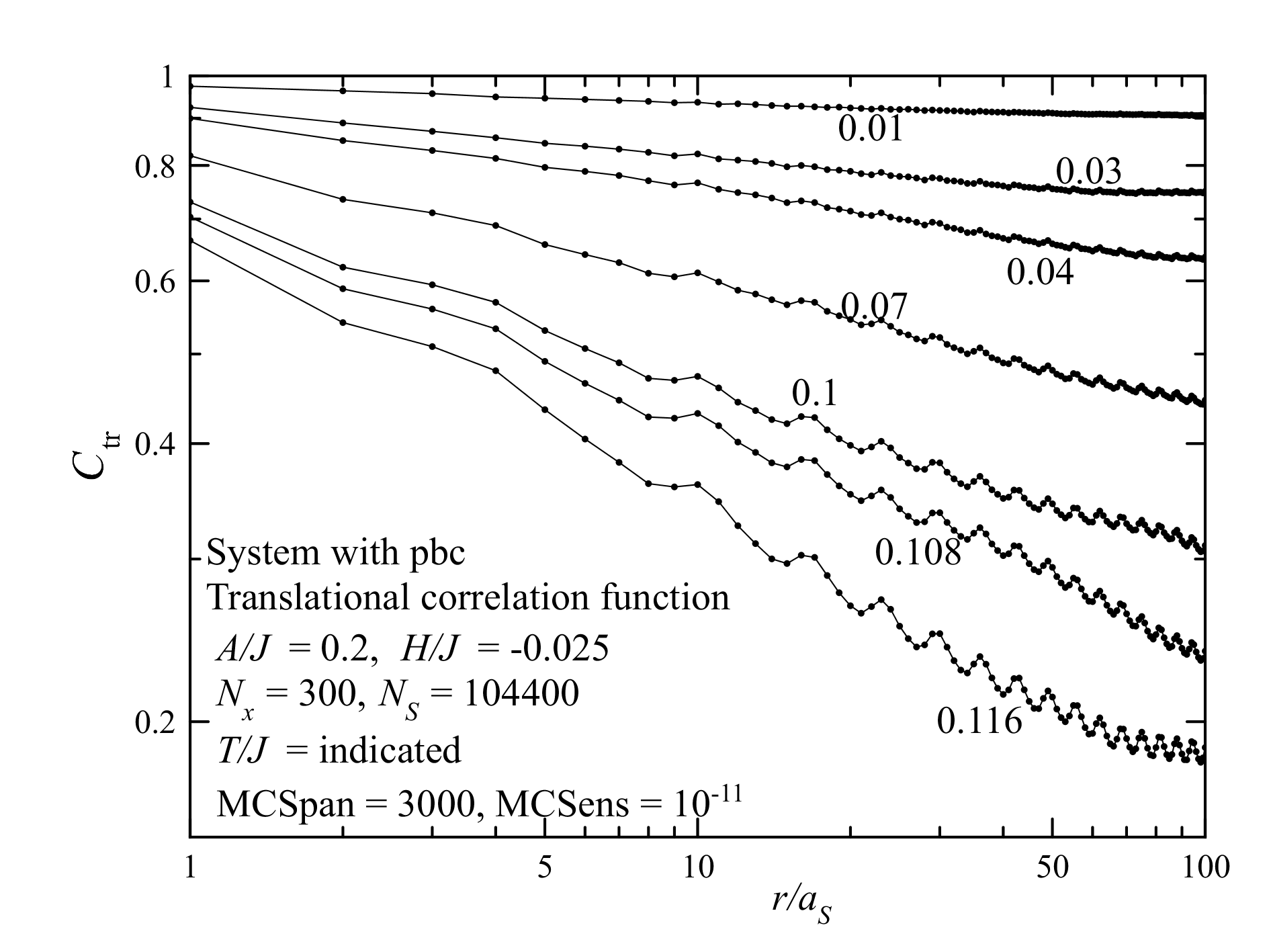
Figure 18: Translational correlation function in the skyrmion lattice at different temperatures.

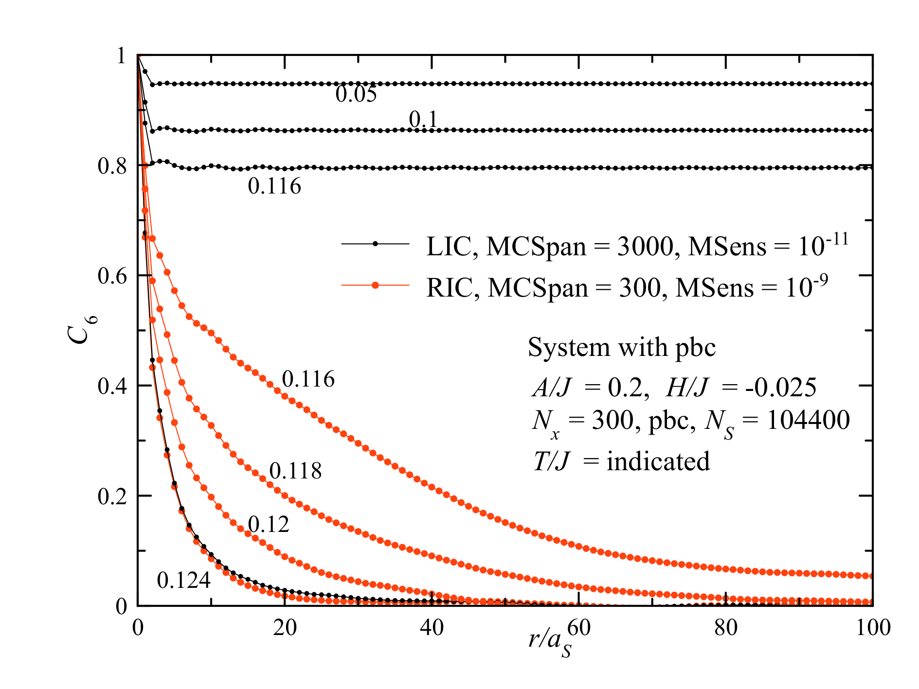
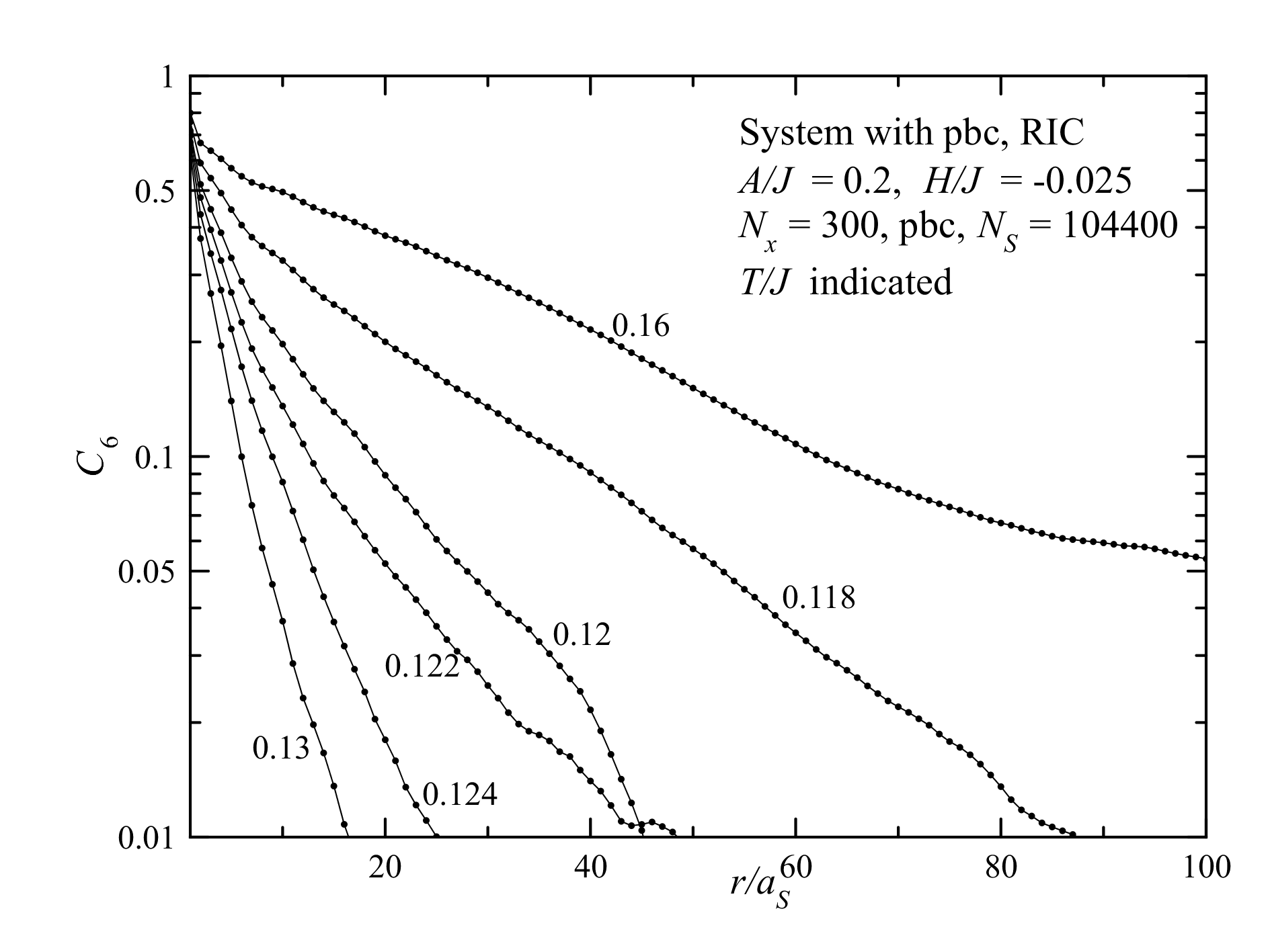
Figure 19: Orientational correlation function in the skyrmion lattice at different temperatures. Upper panel: the results for LIC and RIC in the linear scale. Lower panel: the RIC results in the lin-log scale.

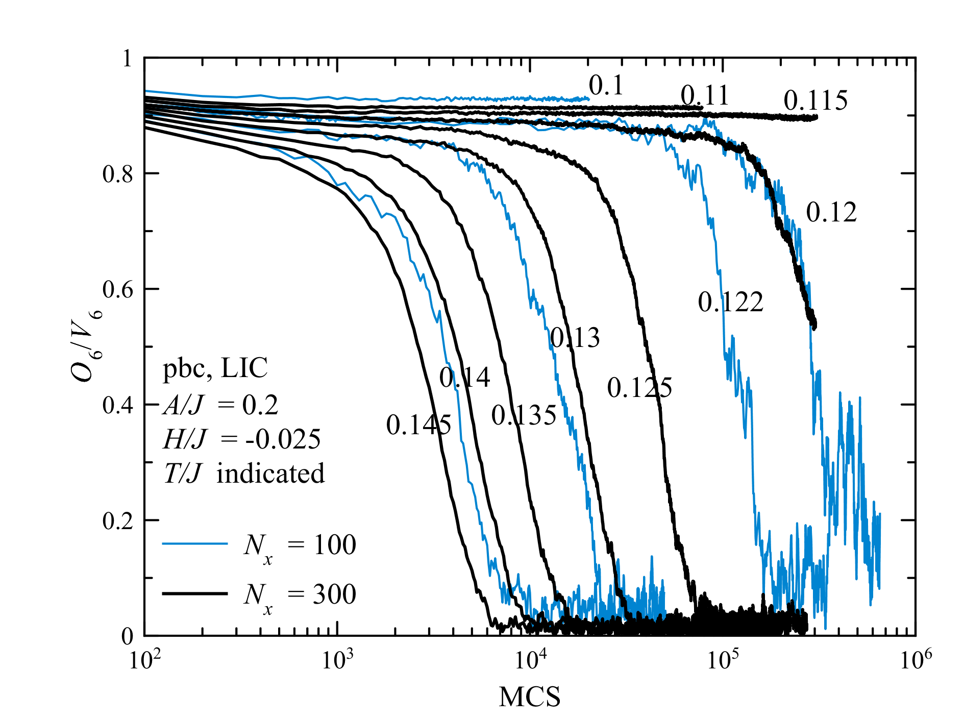
Figure 20: Evolution of the orientational order parameter $O_{6}$ in the course of melting at different temperatures.

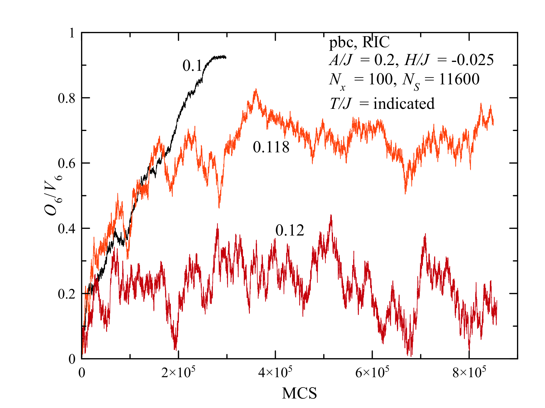
Figure 21: Stationary fluctuations of the orientational order in the polyhexatic phase near the melting transition.

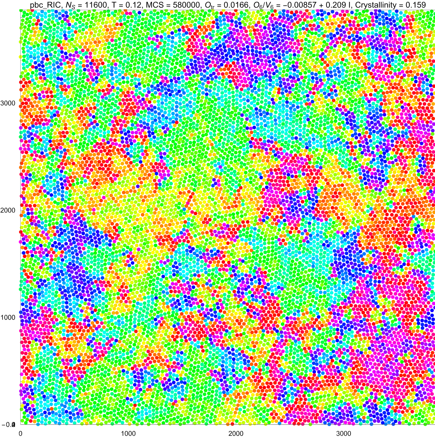
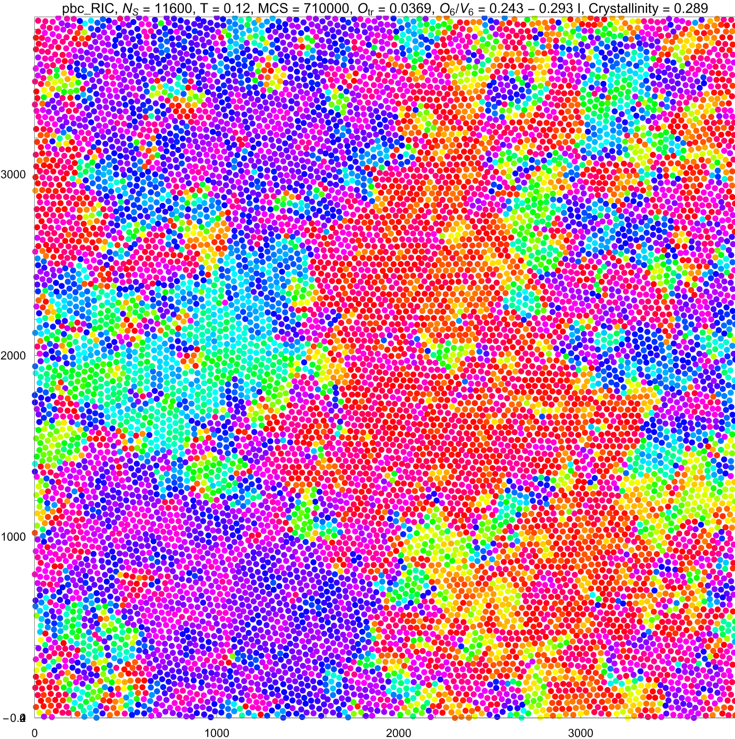
Figure 22: Polyhexatic state at $T/J=0.12$ obtained from RIC in the course of the MC simulation (see Fig. 21). Upper panel: 580000 MCS; Lower panel: 710000 MCS. See the video of the evolution between these states in the Supplemental Materials.

V.2 Correlation functions

The translational correlation function $C_{\mathrm{tr}}(r)$ defined by Eq. (27) makes sense only in the LIC case where the reciprocal-lattice vectors are defined by the perfect lattice used as the initial state [see Eq. (25)]. Cooling the system from the melt leads to a polycrystalline state for which there is no procedure of finding $C_{\mathrm{tr}}(r)$. Formally computing $C_{\mathrm{tr}}(r)$ with the reciprocal-lattice vectors mentioned above leads to $C_{\mathrm{tr}}(r)=0$ everywhere. From the theory of harmonic solids in 2D follows that there is no translational long-range order because it is destroyed by long-wavelength fluctuations. At low temperatures the translational CF decreases as a power of the distance. There is a fair agreement of the numerical data shown in Fig. 18 with the theoretical predictions – the behavior of $C_{\mathrm{tr}}(r)$ is approximately a power law at least up to the distance of a hundred of the skyrmion-lattice periods $a_{S}$. Note that these fair-quality results were obtained with very demanding Monte-Carlo parameters $\mathrm{MCSpan}=3000$ and $\mathrm{MCSense}=10^{-11}$ that results in a large number MCS shown in Fig. 12 (about $5\times 10^{5}$ MCS).

Similar results were obtained in many publications on 2D systems of particles of much smaller sizes, such as $10^{4}$ particles. Our simulations on such small systems yield rather noisy results, especially for CFs. To obtain better results for CFs, one should increase the system size. However, it is difficult to increase the range of distances in which the power law is seen. At long distances correlations are establishing very slowly. One needs to perform an exceedingly large number of MCS to make large portions of the lattice move in different directions to destroy the long-range order and establish power-law correlations. In our simulations, $C_{\mathrm{tr}}(r)$ goes to a plateau at large distances that is an artifact of using a perfect lattice as the initial state. One also can do simulations with pre-heating a lattice up to a higher temperature below the melting point, so that the lattice is not destroyed but translational correlations are strongly suppressed. Then, thermalization at a lower temperature yields a translational CF similar to that obtained with LIC at shorter distances but having random values at larger distances. These considerations show that it is difficult to reproduce the size dependence of the translational quasi-order-parameter, Eq. (29), because for this one needs to know the translational CF at large distances.

The results for the orientational correlation function $C_{6}(r)$, defined by Eq. (20), are shown in Fig. 19 for the LIC and RIC cases. As below the melting point there is a robust orientational long-range order, $C_{6}(r)$ in the LIC case goes to a temperature-dependent plateau. Above the melting point in the LIC case, the behavior of $C_{6}(r)$ changes abruptly and $C_{6}(r)$ goes to zero very quickly. At $T/J=0.124$ there is the same exponential CF in both LIC and RIC cases. Starting from RIC at temperatures below melting, one ends up in a polycrystalline state where $C_{6}(r)$ has a larger range characterizing the size of crystallites. The form of $C_{6}(r)$ here is close to exponential, as can be seen in the lower panel of Fig. 19.

V.3 Evolution of the skyrmion lattice during melting and solidification

In this section we present the time-resolved data on melting and solidification. The role of time is played by the number of Monte Carlo steps (MCS). Both for melting and solidification, there are two stages of the evolution. In the first very fast stage (from 10 to 100 MCS) a partial disordering or partial ordering occurs in the LIC or RIC cases, respectively. These changes are due to the rearrangement of skyrmions at shortest positions.

Then in the RIC case, small grains of the same hexagon orientation emerged as the result of the first stage slowly grow, and larger grains consume smaller ones. This is a very slow process of coarsening via the motion of grain boundaries. Forming a single crystal for large systems takes an exceedingly long time, and in reality this process will be stopped by pinning. The evolution of physical quantities, such as $0_{6}$, in medium-size systems of about $10^{5}$ skyrmions is very irregular as the system is split into only a handful of grains and statistical scatter is very high. To study the coarsening process, a larger system size is needed.

The second stage of melting apparently includes thermal activation. Small grains of different hexagon orientation emerge here and there, then some of them disappear again and some of them grow. Grain boundaries are moving back and forth. Overall, the initially present single crystal breaks up in many smaller crystallites. Evolution of the orientational order parameter in the course of melting at the second stage at different temperatures are shown in Fig. 20. Closer to the melting point, such as at $T/J=0.12$, melting becomes a very slow process, so that no substantial melting occurs before $10^{5}$ MCS.

V.4 The nature of melting and polyhexatic state of the skyrmion lattice

The results of our simulations show that melting of the skyrmion lattice occurs via a first-order phase transition of breaking the lattice into plates of solid, or grains or domains, with different orientations of hexagons. Small grains of different orientations emerge as the result of thermal agitation everywhere in the lattice here and there but at the temperatures below the melting point $T_{m}$ they disappear again as there is an apparent free-energy barrier to overcome for nucleating a surviving grain. The value of $T_{m}$ we obtain slightly decreases on the simulation length, and its best value is $T/J=0.118$, obtained for the system with pbc. As melting is extremely slow, it is difficult to obtain by simulations the true value of $T_{m}$ at which the free energies of the two phases become equal to each other and melting time becomes infinite.

The phase above the melting point is not yet a liquid phase because of a significant size of grains of solid. With increasing the temperature, these grains become smaller and the system approaches the liquid state. With lowering the temperature, the grains grow in size. This coarsening process is very slow and does not lead to a single crystal for large systems or for systems with frustrating boundaries. The resulting state at low temperatures is polycrystalline, as shown on Fig. 9.

In the temperature region near the melting point, the state with large grains of solid is thermodynamically stable and shows eqiulibrium fluctuations in which boundaries between the grains are moving back and forth (see a video of the evolution of the polyhexatic state at $T/J=0.12$ in the course of MC simulation in Supplemental Materials). With time, the shape of the grains changes significantly but, on average, they do not become larger or smaller, see Fig. 21. We call this state polyhexatic state. The polyhexatic phase in the system with pbc near melting is shown in Fig. 22 at two different moments of the MC simulation. The video of the evolution between these two states can be found in the Supplemental Materials.

VI Conclusions

In this paper, a simplified approach to the skyrmion lattice is proposed that is based on the skyrmion’s core energy and the recently established exponential repulsion of skyrmions [63]. With these two components, one can find the equilibrium concentration of skyrmions, that is, the period of the skyrmion lattice $a_{S}$. After that, the number of skyrmions can be fixed as the processes of skyrmion creation/annihilation are rare at low temperatures where the melting of the skyrmion lattice takes place. Thus, one can consider skyrmions as interacting particles and use Monte Carlo or other methods to describe their properties. This approach is much simpler than considering the system in terms of spins on the lattice [58].

The results obtained point to a first-order transition of breaking a single-crystal lattice into the polyhexatic state of large grains with different orientations of hexagons. With increasing/decreasing the temperature these grains shrink/grow. The polyhexatic state differs from the polycrystalline state at $T=0$ by the equilibrium thermal fluctuations that change its shape.

We haven’t observed two transitions with an intermediate state with a power-law dependence of the orientational correlation function. In the single-crystal state below melting, this CF has a plateau while in the polyhexatic state its decay with the distance is closer to exponential. The CF data near melting are not that accurate because the ratio of the grain size to the system size is not small enough. Better results could be obtained with a larger system size. In numerical work, the direct checking of the KTHNY scenario of the unbinding of dislocation pairs, followed by the dissociation of disinclination pairs, is hampered by the difficulty to identify dislocations and disclinations because at elevated temperatures thermal fluctuations create significant non-topological local distortions of the crystal lattice.

Over the period of forty years, there has been a significant controversy over the KTHNY scenario in real and numerical experiments, including the most recent work on skyrmion lattices. Some of it reflects the differences in the interactions of particles forming the crystal and the differences in the crystal symmetry [53-57]. Our results demonstrate the importance of another factor that is always present in real and numerical experiments on melting and solidification - nonequlibrium effects. Real solids rarely form monocrystals. This is true in both 3D and 2D. When the numerical experiment is performed on a large system, and it resembles real experiment in a sense that the solid is formed by freezing the liquid, the most common practical result is a polycrystalline state in which global orientational order is lost. Similarly, when a sufficiently large 2D crystal melts, there is no guarantee that the resulting state would be homogeneous with, e.g, power-law decay of orientational correlations. As our work demonstrates, it consists of differently oriented domains of the Halperin-Nelson hexatic phase, which we call a polyhexatic state. Same as for a polycrystalline state, the orientational order in the polyhexatic state is limited to the size of the domain. The average size of the fluctuating hexatic domain goes down on raising temperature above the melting transition, leading to a fully disordered liquid state at high temperature.

Quenched disorder is known to have a stronger effect on long-range correlations than thermal fluctuations. It has been shown that for a 2D atomic layer on a substrate, the defects in the substrate can generate a hexatic state characterized by short-range translational order and algebraic decay of the orientational order even at zero temperature [65, 67, 68]. Thus, monocrystallinity of the skyrmion lattice may not be sufficient in search for the temperature-induced hexatic phase. The perfection of the underlying atomic lattice must be pursued as well.

We hope that further experiments on skyrmion lattices will shed light on the existence of polycrystalline and polyhexatic 2D phases investigated in this paper.

VII Acknowledgments

This work has been supported by the grant No. DE-FG02-93ER45487 funded by the U.S. Department of Energy, Office of Science.

References

- [1] T. H. R. Skyrme, A non-linear theory of strong interactions, Proceedings of the Royal Society A 247, 260-278 (1958).
- [2] A. M. Polyakov, Gauge Fields and Strings, Harwood Academic Publishers 1987.
- [3] N. Manton and P. Sutcliffe, Topological Solitons, Cambridge University Press 2004.
- [4] E. Braaten and L. Carson, Deuteron as a toroidal skyrmion, Physical Review D 38, 3525-3539 (1988).
- [5] W. Y. Crutchfield, N. J. Snyderman, and V. R. Brown, Deuteron in the Skyrme model, Physical Review Letters 68, 1660-1662 (1992).
- [6] N. Nagaosa and Y. Tokura, Topological properties and dynamics of magnetic skyrmions, Nature Nanotechnology 8, 899-911 (2013).
- [7] X. Zhang, M. Ezawa, and Y. Zhou, Magnetic skyrmion logic gates: conversion, duplication and merging of skyrmions, Scientific Reports 5, 9400-(8) (2015).
- [8] G. Finocchio, F. Büttner, R. Tomasello, M. Carpentieri, and M. Klaui, Magnetic skyrmions: from fundamental to applications, Journal of Physics D: Applied Physics. 49, 423001-(17) (2016).
- [9] W. Jiang, G. Chen, K. Liu, J. Zang, S. G. E. te Velthuis, and A. Hoffmann, Skyrmions in magnetic multilayers, Physics Reports 704, 1-49 (2017).
- [10] A. Fert, N. Reyren, and V. Cros, Magnetic skyrmions: advances in physics and potential applications, Nature Reviews Materials 2, 17031-(15) (2017).
- [11] A. P. Malozemoff and J. C. Slonczewski, Magnetic Domain Walls in Bubble Materials, Academic Press 1979.
- [12] T. H. O’Dell, Ferromagnetodynamics: The Dynamics of Magnetic Bubbles, Domains, and Domain Walls, Wiley 1981.
- [13] A. A. Belavin and A. M. Polyakov, Metastable states of two-dimensional isotropic ferromagnets, Pis’ma Zh. Eksp. Teor. Fiz 22, 503-506 (1975) [JETP Lett. 22, 245-248 (1975)].
- [14] E. M. Chudnovsky and J. Tejada, Lectures on Magnetism, Rinton Press (Princeton - NJ, 2006).
- [15] L. Cai, E. M. Chudnovsky, and D. A. Garanin, Collapse of skyrmions in two-dimensional ferromagnets and antiferromagnets, Physical Review B 86, 024429-(4) (2012).
- [16] M. Ezawa, Giant skyrmions stabilized by dipole-dipole interactions in thin ferromagnetic films, Physical Review Letters 105, 197202-(4) (2010).
- [17] I. Makhfudz, B. Krüger, and O. Tchernyshyov, Inertia and chiral edge modes of a skyrmion magnetic bubble, Physical Review Letters 109, 217201-(4) (2012).
- [18] A. N. Bogdanov and D. A. Yablonskii, Thermodynamically stable “vortices” in magnetically ordered crystals. The mixed state of magnets. Soviet Physics JETP 68, 101-103 (1989).
- [19] A. Bogdanov and A. Hubert, Thermodynamically stable magnetic vortex states in magnetic crystals, J. Magn. Magn. Mater. 138, 255-269 (1994).
- [20] U. K. Rößler, N. Bogdanov, and C. Pfleiderer, Spontaneous skyrmion ground states in magnetic metals, Nature 442, 797-801 (2006).
- [21] S. Heinze, K. von Bergmann, M. Menzel, J. Brede, A. Kubetzka, R. Wiesendanger, G. Bihlmayer, and S. Blugel, Spontaneous atomic-scale magnetic skyrmion lattice in two dimensions, Nature Physics 7, 713-718 (2011).
- [22] O. Boulle, J. Vogel, H. Yang, S. Pizzini, D. de Souza Chaves, A. Locatelli, T. O. Mentes, A. Sala, L. D. Buda-Prejbeanu, O. Klein, M. Belmeguenai, Y. Roussigné, A. Stahkevich, S. M. Chérif, L. Aballe, M. Foerster, M. Chshiev, S. Auffret, I. M. Miron, and G. Gaudin, Room-temperature chiral magnetic skyrmions in ultrathin magnetic nanostructures, Nature Nanotechnology 11, 449-454 (2016).
- [23] A. O. Leonov, T. L. Monchesky, N. Romming, A. Kubetzka, A. N. Bogdanov, and R. Wiesendanger, The properties of isolated chiral skyrmions in thin magnetic films, New Journal of Physics 18, 065003-(16) (2016).
- [24] A. O. Leonov and M. Mostovoy, Multiply periodic states and isolated skyrmions in an anisotropic frustrated magnet, Nature Communications 6, 8275-(8) (2015).
- [25] X. Zhang, J. Xia, Y. Zhou, X. Liu, H. Zhang, and M. Ezawa, Skyrmion dynamics in a frustrated ferromagnetic film and current-induced helicity locking-unlocking transition, Nature Communications 8 1717-(10) (2017).
- [26] B. A. Ivanov, A. Y. Merkulov, V. A. Stepanovich, C. E. Zaspel, Finite energy solitons in highly anisotropic two dimensional ferromagnets, Physical Review B 74, 224422-(17) (2006).
- [27] S.-Z. Lin and S. Hayami, Ginzburg-Landau theory for skyrmions in inversion-symmetric magnets with competing interactions, Physical Review B 93, 064430-(16) (2016).
- [28] E. M. Chudnovsky and D. A. Garanin, Skyrmion glass in a 2D Heisenberg ferromagnet with quenched disorder, New Journal of Physics 20 033006-(9) (2018).
- [29] C. Moutafis, S. Komineas, and J. A. C. Bland, Dynamics and switching processes for magnetic bubbles in nanoelements, Physical Review B 79, 224429-(8) (2009).
- [30] P. F. Bessarab, G. P. Müller, I. S. Lobanov, F. N. Rybakov, N. S. Kiselev, H. Jansson, V. M. Uzdin, S. Blügel, L. Bergqvist, and A. Delin, Lifetime of racetrack skyrmions, Nature Scientific Reports 8, 3433-(10) (2018).
- [31] D. Stosic, J. Mulkers, B. Van Waeyenberge, T. B. Ludermir, and M. V. Milosevic, Paths to collapse for isolated skyrmions in few-monolayer ferromagnetic films, Physical Review B 95, 214418-(12) (2017).
- [32] L. Desplat, D. Suess, J-V. Kim, and R. L. Stamps, Thermal stability of metastable magnetic skyrmions: Entropic narrowing and significance of internal eigenmodes, Physical Review B 98, 134407-(13) (2018).
- [33] J. Hagemeister, N. Romming, K. von Bergmann, E. Y. Vedmedenko, and R. Wiesendanger, Stability of single skyrmionic bits, Nature Communications 6, 8455-(7) (2015).
- [34] S. Rohart, J. Miltat, and A. Thiaville, Path to collapse for an isolated Néel skyrmion, Physical Review B 93, 214412-(6) (2016).
- [35] L. Rozsa, E. Simon, K. Palotás, L. Udvardi, and L. Szunyogh, Complex magnetic phase diagram and skyrmion lifetime in an ultrathin film from atomistic simulations, Physical Review B 93, 024417-(10) (2016).
- [36] A. Siemens, Y. Zhang, J. Hagemeister, E. Y. Vedmedenko, and R. Wiesendanger, Minimal radius of magnetic skyrmions: statics and dynamics, New Journal of Physics 18 045021-(9) (2016).
- [37] S. von Malottki, P. F. Bessarab, S. Haldar, A. Delin, and S. Heinze, Skyrmion lifetime in ultrathin films, Physical Review B 99, 060409(R)-5 (2019).
- [38] A. Derras-Chouk, E. M. Chudnovsky, and D. A. Garanin, Thermal collapse of a skyrmion, Journal of Applied Physics 126, 083901-(7) (2019).
- [39] M. Hoffmann, G. P. Müller, and S. Blügel, Atomistic perspective of long lifetimes of small skyrmions at room temperature, Physical Review Letters 124, 247201-(5) (2020).
- [40] X. Yu, Y. Onose, N. Kanazawa, J. Park, J. Han, Y. Matsui, N. Nagaosa, and Y. Tokura, Real-space observation of a two-dimensional skyrmion crystal, Nature 465, 901 - 904 (2010).
- [41] D. A. Garanin, E. M. Chudnovsky, S. Zhang, and X. X. Zhang, Thermal creation of skyrmions in ferromagnetic films with perpendicular anisotropy and Dzyaloshinskii-Moriya interaction, Journal of Magnetism and Magnetic Materials 493, 165724-(9).
- [42] T. Dohi, R. M. Reeve, and M. Kläui, Thin film skyrmionics, Annual Review of Condensed Matter Physics 33, 73-95 (2022).
- [43] B. I. Halperin and D. R. Nelson, Theory of two-dimensional melting, Physical Review Letters 41, 121-124 (1978).
- [44] D. R. Nelson and B. I. Halperin, Dislocation-mediated melting in two dimensions, Physical Review B 19, 2457-2483 (1979). ,
- [45] A. P. Young, Melting and the vector Coulumb gas in two dimensions, Physical Review B 19, 1855-1866 (1979).
- [46] K. J. Strabdburg, Two-dimensional melting, Review of Modern Physics 60, 161-207 (1988).
- [47] J. M. Kosterlitz and D. J. Thouless, Ordering, metastability and phase transitions in two-dimensional systems, Journal of Physics C: Solid State Physics 6, 1181-1203 (1973).
- [48] R. Dickman and E. M. Chudnovsky, Elastic lattice in an incommensurate background, Physical Review B 51, 97-106 (1995).
- [49] Y.-W. Li and M. Pica Ciamara, Accurate determination of the translational correlation function of two-dimensional solids, Physical Review E 100, 062606-(6)(2019).
- [50] C. A. Murray, W. O. Sprenger, and R. A. Wenk, Comparison of melting in three and two dimensions: Microscopy of colloidal spheres, Physical Review B 42, 688-703 (1990).
- [51] H. H. von Grünberg, P. Keim, and G. Maret, Phase transitions in two-dimensional colloidal systems, Chapter 2, pp. 40-83 in Soft Matter, Volume 3: Colloidal Order: Entropic and Surface Forces, edited by G. Gompper and M. SchickWeinheim : WILEY-VCH, 2007 - ISBN 978-3-527-31370-9.
- [52] E. Zeldov, D. Majer, M. Konczykowski, V. B. Geshkembein, V. M. Vinokur, and H. Shtrickman, Thermodynamic observation of first-order vortex-lattice melting transition in Bi2Sr2CaCu2O8, Nature 375, 373-376 (1995).
- [53] J. Q. Broughton, G. H. Gilmer, and J. D. Weeks, Molecular-dynamics study of melting in two dimensions: Inverse-twelfth-power interaction, Physical Review B 25, 4651-4669 (1982).
- [54] E. N. Tsiok, Y. D. Fomin, E. A. Gaiduk, E. E. Tareyeva, V. N. Ryzhov, P. A. Libet, N. A. Dmitryuk, N. P. Kryuchkov, and S. O. Yurchenko, Journal of Chemical Physics 156, 114703-(11) (2022).
- [55] S. C. Kapfer and W. Krauth, Physical Review Letters 114, 035702 (2015).
- [56] W. Janke and H. Kleinert, From first-order to two continuous melting transitions: Monte Carlo Study of a new 2D lattice-defect model, Physical Review Letters 61, 2344-2347 (1988); Erratum Physical Review Letters 62, 608 (1989).
- [57] J. Dietel and H. Kleinert, Triangular lattice model of two-dimensional defect melting, Physical Review B 73, 024113 (2006).
- [58] Y. Nishikawa, K. Hukushima, and W. Krauth, Solid-liquid transition of skyrmions in a two-dimensional chiral magnet, Physical Review B 99, 064435 (2019).
- [59] P. Huang, T. Schönenberger, M. Cantoni, L. Heinen, A. Magrez, A. Rosch, F. Carbone, and H. M. Rønnow, Melting of a skyrmion lattice to a skyrmion liquid via a hexatic phase, Nature Nanotechnology 15, 761-767 (2020).
- [60] P. Baláž, M. Paściak, and J. Hlinka, Melting of Néel skyrmion lattice, Physical Review B 103, 174411-(8) (2021).
- [61] J. Zazvorka, F. Dittrich, Y. Ge, N. Kerber, K. Raab, T. Winkler, K. Litzius, M. Veis, P. Virnau, and M. Kläui, Skyrmion lattice phases in thin film multilayer, Advanved Functional Materials 30, 2004037-(8) (2020).
- [62] A. R. C. McCray, Y. Li, R. Basnet, K. Pandey, J. Hu, D. Phelan, X. Ma, A. K. Petford-Long, and C. Phatak, Thermal hysteresis behavior of skyrmion lattices in the van der Waals Ferromagnet Fe3GeTe2, arXiv:2203.02666.
- [63] D. Capic, D. A. Garanin, and E. M. Chudnovsky, Skyrmion-skyrmion interaction in a magnetic film, Journal of Physics: Condensed Matter 32, 415803-(14) (2020).
- [64] A. Derras-Chouk, E. M. Chudnovsky, and D. A. Garanin, Quantum collapse of a magnetic skyrmion, Physical Review B 98, 024423-(9) (2018)
- [65] E. M. Chudnovsky, Structure of a solid film on an imperfect surface, Physical Review B 33, 245-250 (1986).
- [66] E. M. Chudnovsky, Hexatic vortex glass in disordered superconductors, Physical Review B 40, 11355(R)-11357(R) (1989).
- [67] C. A. Murray, P. L. Gammel, D. J. Bishop, D. M. Mitzi, and A. Kapitulnik, Observation of a hexatic vortex glass in flux lattices of the high- superconductor Bi2.1Sr1.9Ca0.9Cu2O8+δ, Physical Review Letters 64, 2312-2315 (1990).
- [68] E. M. Chudnovsky and R. Dickman, Elastic lattice in a random potential, Physical Review B 57, 2724-2727 (1998).